author

The Quantum Random Energy Model
as a Limit of p-Spin Interactions

Abstract We consider the free energy of a mean-field quantum spin glass described by a $p$-spin interaction and a transversal magnetic field. Recent rigorous results for the case $p=\infty$, i.e. the quantum random energy model (QREM), are reviewed. We show that the free energy of the $p$-spin model converges in a joint thermodynamic and $p\to\infty$ limit to the free energy of the QREM.

1 Introduction

A prominent class of classical mean-field spin glass models are $p$-spin interactions defined on $N$ Ising-type spins

$$\boldsymbol{\sigma}=(\sigma_{1},\dots,\sigma_{N})\in\{-1,1\}^{N}=:\mathcal{Q}_{N}.$$ (1.1)

For fixed $p\in[1,\infty)$ the interaction energy of these spins is random and given by

$$U_{p}(\boldsymbol{\boldsymbol{\sigma}})=\frac{1}{N^{\frac{p-1}{2}}}\sum_{j_{1},\dots,j_{p}=1}^{N}g_{j_{1},\dots,j_{p}}{\sigma}_{j_{1}}\cdots{\sigma}_{j_{p}}$$ (1.2)

in terms of an array $g_{\boldsymbol{j}}:=g_{j_{1},\dots,j_{p}}$ of independent and identically distributed (i.i.d.), centered Gaussian random variable with variance one. The process $U_{p}(\boldsymbol{\sigma})$, $\boldsymbol{\sigma}\in\mathcal{Q}_{N}$ is then Gaussian as well and uniquely characterized by its mean and covariance function,

$$\mathbb{E}\left[U_{p}(\boldsymbol{\sigma})\right]=0,\qquad\mathbb{E}\left[U_{p}(\boldsymbol{\sigma})U_{p}(\boldsymbol{\sigma}^{\prime})\right]=N\left(N^{-1}\sum_{j=1}^{N}\sigma_{j}\sigma_{j}^{\prime}\right)^{p}=:N\,\xi(\boldsymbol{\sigma},\boldsymbol{\sigma}^{\prime})^{p}.$$ (1.3)

The special case $p=2$ corresponds to the Sherrington-Kirkpatrick model, and in the limit $p\to\infty$ we obtain Derrida’s random energy model (REM) [1]. In the latter case, the correlations vanish and the variables $U_{\infty}(\boldsymbol{\sigma})$ form an i.i.d. Gaussian process on the hypercube $\mathcal{Q}_{N}$.

There is a wealth of results both in the physics as well as mathematics literature concerning properties of the Gibbs measure of these classical mean-field spin glasses. Most celebrated is a closed form expression for the free energy derived by Parisi [2] and later proven by Talagrand and Panchenko [3, 4]. This formula reflects the fact that at low temperatures the Gibbs measure fractures into many inequivalent pure states. A key quantity in this area is the distribution of the overlap $\xi(\boldsymbol{\sigma},\boldsymbol{\sigma}^{\prime})$ of independent copies or replicas of spins $\boldsymbol{\sigma},\boldsymbol{\sigma}^{\prime}$. We refer the mathematically interested reader to the monographs [5, 6, 7] and references therein.

Despite its popularity in physics (cf. [8, 9] and refs. therein), much less is rigorously established if one incorporates quantum effects in the form of a transversal magnetic field. In the quantum case, one views the spins configurations (1.1) as the $z$-components of $N$ spin-$1/2$ quantum spins and the energy (1.2) is lifted to the corresponding Hilbert space $\otimes_{j=1}^{N}{\mathbb{C}}^{2}\equiv\ell^{2}(\mathcal{Q}_{N})$ as a diagonal matrix $U_{p}$. The random Hamiltonian of the quantum p-spin model with transversal magnetic field of strength $\Gamma\geq 0$ is

$$H_{p}=U_{p}+\Gamma\,T,$$ (1.4)

where $\left(T\psi\right)(\boldsymbol{\sigma}):=-\sum_{j=1}^{N}\psi(\sigma_{1},\dots,-\sigma_{j},\dots,\sigma_{N})$ coincides with the action of the negative sum of $x$-components of the Pauli matrices in the $z$-basis. In this paper, we are concerned with the corresponding quantum free energy or pressure at inverse temperature $\beta\in[0,\infty)$

$$\Phi_{N}^{p}(\beta,\Gamma):=\frac{1}{N}\ln Z_{N}^{p}(\beta,\Gamma)$$ (1.5)

which derives from the partition function $Z_{N}^{p}(\beta,\Gamma)=2^{-N}{\operatorname{Tr}\,}e^{-\beta H_{p}}$. The case $p=\infty$ corresponds to the pressure of the quantum random energy model (QREM), and we will write $\Phi^{\text{QREM}}(\beta,\Gamma):=\Phi^{\infty}(\beta,\Gamma)$.

2 Rigorous results on the free energy

A basic property of the free energy of spin glasses is its self-averaging, i.e. the fact that in the thermodynamic limit $N\to\infty$ this quantity agrees almost surely with its average. For p-spin interactions even more general than (1.2) self-averaging of the quantum free energy has been established in [10]. Since we restrict ourselves to the Gaussian case, this property follows immediately from the standard Gaussian concentration inequality. We therefore include the short argument for pedagogical reasons.

Proposition 2.1 ([10]).

There are some constants $c,C\in(0,\infty)$ such that for any $p\in[1,\infty]$ the Gaussian concentration estimate

$$\mathbb{P}\left(\left|\Phi_{N}^{p}(\beta,\Gamma)-\mathbb{E}\left[\Phi_{N}^{p}(\beta,\Gamma)\right]\right|>\frac{t\,\beta}{\sqrt{N}}\right)\leq C\,\exp\left(-ct^{2}\right)$$ (2.1)

holds for all $t>0$ and all $N\in\mathbb{N}$ .

Proof.

The pressure’s variations with respect to the i.i.d. standard Gaussian variables $g_{\boldsymbol{j}}$ is

$$-\frac{\partial\Phi_{N}^{p}(\beta,\Gamma)}{\partial g_{\boldsymbol{j}}}=\frac{\beta}{N^{\frac{p+1}{2}}\,2^{N}Z(\beta,\Gamma)}\sum_{\boldsymbol{\sigma}}\sigma_{j_{1}}\cdots{\sigma}_{j_{p}}\,\langle\boldsymbol{\sigma}|e^{-\beta H}|\boldsymbol{\sigma}\rangle.$$

Here and in the following we use Dirac’s bracket notation for matrix elements. Consequently, the Lipschitz constant is bounded by

$$\sum_{\boldsymbol{j}}\left(\frac{\partial\Phi_{N}^{p}(\beta,\Gamma)}{\partial g_{\boldsymbol{j}}}\right)^{2}\leq\frac{\beta^{2}}{N}.$$

The claim thus follows from the Gaussian concentration inequality for Lipschitz functions. ∎

In the classical case $\Gamma=0$, the free energy of any $p$-spin interaction is given in terms of Parisi’s formula [4]. One of its main features is a transition at small enough temperatures to a spin glass regime. At $p=\infty$ this formula takes a simple form:

$$\Phi^{\text{REM}}(\beta)=\lim_{N\to\infty}\Phi_{N}^{\infty}(\beta,0)=\left\{\begin{array}[]{l@{\quad}r}\tfrac{1}{2}\beta^{2}&\mbox{if }\;\beta\leq\beta_{c},\\[4.30554pt] \tfrac{1}{2}\beta_{c}^{2}+(\beta-\beta_{c})\beta_{c}&\mbox{if }\;\beta>\beta_{c}.\end{array}\right.$$ (2.2)

The non-differentiability at

$$\beta_{c}:=\sqrt{2\ln 2}$$

reflects a first-order freezing transition into a low-temperature phase characterized by the vanishing of the specific entropy.

Under the addition of a constant transversal field, this freezing transition vanishes for $\Gamma$ large enough. A first-order phase transition into a quantum paramagnetic phase, characterized by

$$\Phi^{\mathrm{PAR}}(\beta\Gamma):=\ln\cosh\left(\beta\Gamma\right),$$

occurs at $\Gamma_{c}(\beta):=\beta^{-1}\operatorname{arcosh}\left(\exp\left(\Phi^{\text{REM}}(\beta)\right)\right)$. At $\beta=\infty$ this connects to the known location $\Gamma_{c}(\infty)=\beta_{c}$ of the quantum phase transition of the ground state [11, 12].

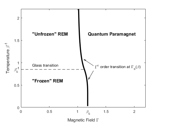
Figure 1: Phase diagram of the QREM as a function of the transversal magnetic field $\Gamma$ and the temperature $\beta^{-1}$. The first-order transition occurs at fixed $\beta$ and $\Gamma_{c}(\beta)$. The freezing transition is found at temperature $\beta_{c}^{-1}=(2\ln 2)^{-1/2}$, which is unchanged in the presence of a magnetic field of strength $\Gamma<\Gamma_{c}(\beta)$.

The shape of the phase diagram of the QREM in Figure 1 including the precise location of the first-order transition, was predicted by Goldschmidt [13] in the 1990s. His arguments are based on the replica trick and the so-called static approximation in the path-integral representation of ${\mathbb{E}\,}[Z_{N}^{p}(\beta,\Gamma)^{n}]$. In a recent paper [14], we confirmed this prediction.

Theorem 2.2 ([14]).

For any $\Gamma,\beta\geq 0$ almost surely:

$$\Phi^{\text{QREM}}(\beta,\Gamma):=\lim_{N\to\infty}\Phi_{N}^{\textrm{QREM}}(\beta,\Gamma)=\max\{\Phi^{\text{REM}}(\beta),\Phi^{\text{PAR}}(\beta\Gamma)\}.$$

In broad terms, the main features of the phase diagram in Figure 1 such as a low-temperature frozen phase which gives way to a paramagnetic phase at both high temperatures or strong magnetic field are expected to stay for general $p$; cf. [13, 15, 16, 8]. The new features for general $p$ are the richer structure of the low-temperature phase due to higher-order replica symmetry breaking and the conjectured endpoint of the first-order transition line in a critical point at a finite temperature which scales with $\sqrt{p}$. No closed expression for the free energy is known in the quantum case. Crawford [10] showed that the almost-sure limit

$$\Phi^{p}(\beta,\Gamma):=\lim_{N\to\infty}\Phi_{N}^{p}(\beta,\Gamma),$$ (2.3)

exists for any $p\in[1,\infty]$. All claims concerning the structure of the phase diagram for quantum p-spin models are based on non-rigorous calculations using the replica trick and a $1/p$ expansion [13, 15, 16]. In fact, it is widely believed that $\Phi^{p}(\beta,\Gamma)$ is continuous in $1/p$ and hence tends to the explicit expression for the QREM,

$$\lim_{p\to\infty}\Phi^{p}(\beta,\Gamma)=\Phi^{\textrm{QREM}}(\beta,\Gamma).$$

We do not quite proof this conjecture in this paper. However, as a main new result we have the following continuity of the free energy.

Theorem 2.3.

Let $p(N)$ be a nonnegative sequence which satisfies a superlogarithmic growth condition, i.e.

$$\lim_{N\to\infty}\frac{p(N)}{\ln(N)}=\infty.$$ (2.4)

For any $\beta,\Gamma\geq 0$, we then have the almost sure convergence

$$\lim_{N\to\infty}\Phi_{N}^{p(N)}(\beta,\Gamma)=\Phi^{\text{QREM}}(\beta,\Gamma).$$ (2.5)

The proof of this statement heavily relies on the method of proof of Theorem 2.2 in [14]. It will be presented in Section 3 below.

Let us conclude with some remarks:

1. In the classical case $\Gamma=0$, the quenched pressure $\mathbb{E}\left[\Phi_{N}^{p}(\beta,0)\right]$ is monotonically increasing in $p$ and, in particular, we have $\mathbb{E}\left[\Phi_{N}^{p}(\beta,0)\right]\leq\mathbb{E}\left[\Phi_{N}^{\textrm{REM}}(\beta)\right]$ for any $N\in\mathbb{N}$. This follows with the help of Gaussian comparison [5, Lemma 10.2.1] from the following facts: i) $2{\mathbb{N}}\ni p\mapsto\mathbb{E}\left[U_{p}(\boldsymbol{\sigma})U_{p}(\boldsymbol{\sigma}^{\prime})\right]$ is monotonically decreasing, and ii) $\frac{\partial^{2}\Phi_{N}^{p}(\beta,0)}{\partial U_{p}(\boldsymbol{\sigma})\partial U_{p}(\boldsymbol{\sigma}^{\prime})}<0$ in case $\boldsymbol{\sigma}\neq\boldsymbol{\sigma}^{\prime}$. Unfortunately, a similar monotonicity is not known in the quantum case.

2. Another intensively studied family of mean-field spin-glasses are the so-called spherical $p$-spin models, given by

   $$\widehat{U}_{p}(\boldsymbol{\boldsymbol{\sigma}})=\sqrt{\frac{p!}{N^{p-1}}}\sum_{1\leq j_{1}<\dots<j_{p}\leq N}g_{j_{1},\dots,j_{p}}{\sigma}_{j_{1}}\cdots{\sigma}_{j_{p}}.$$ (2.6)

   In the classical case the spherical $p$-spin models give rise to the same pressure in the thermodynamic limit as the $p$-spin SK-models (1.2); however, the models have different scales of fluctuations [17].
   Theorem 2.3 remains true (with minor changes in the proof) if one works instead with the spherical $p$-spin models. This follows from the observation that

   $$\mathbb{E}\left[\widehat{U}_{p}(\boldsymbol{\sigma})\widehat{U}_{p}(\boldsymbol{\sigma}^{\prime})\right]=N\,(\xi(\boldsymbol{\sigma},\boldsymbol{\sigma}^{\prime})^{p}-\delta_{N}^{p}(\boldsymbol{\sigma},\boldsymbol{\sigma^{\prime}})),$$ (2.7)

   where $\delta_{N}^{p}(\boldsymbol{\sigma},\boldsymbol{\sigma^{\prime}})$ is uniformly bounded,

   $$|\delta_{N}^{p}(\boldsymbol{\sigma},\boldsymbol{\sigma^{\prime}})|\leq\frac{1}{N^{p}}\sum_{\begin{subarray}{c}1\leq j_{1}\leq\dots\leq j_{p}\leq N\\ \exists 1\leq k<l\leq p:\,j_{k}=j_{l}\end{subarray}}1\leq\frac{N^{p}-p!\binom{N}{p}}{N^{p}}\leq\min\left\{1,\frac{p(p-1)}{2N}\right\}.$$ (2.8)

3 Proof of Theorem 2.3

The proof is an adaptation of the strategy for the proof Theorem 2.2 in [14]. The lower bound in [14] was based on the Gibbs variational principle and established there already for general p-spin interactions. For convenience of the reader, we recall the corresponding lemma here.

Lemma 3.1 (=Lemma 2.1 in [14]).

For any $p\in[1,\infty]$, $N\in\mathbb{N}$ and $\Gamma,\beta\geq 0$:

$$\Phi_{N}^{p}(\beta,\Gamma)\geq\max\left\{\Phi_{N}^{p}(\beta,0),p^{\mathrm{PAR}}(\beta\Gamma)-\frac{\beta}{N2^{N}}\sum_{\boldsymbol{\sigma}\in\mathcal{Q}_{N}}U_{p}(\boldsymbol{\sigma})\right\}.$$ (3.1)

The main new challenge is to cope with the correlations in $U_{p}$ for $p<\infty$ in the upper bound of [14]. Since these correlations vanish in the limit $p\to\infty$, the large deviation sets

$$\mathcal{L}_{\epsilon}^{p}\coloneqq\{\boldsymbol{\sigma}|U_{p}(\boldsymbol{\sigma})<-\epsilon N\},$$ (3.2)

with $\epsilon>0$ are expected to consist of isolated small clusters. We write $\mathcal{L}_{\epsilon}^{p}=\bigcup_{\alpha}C_{\epsilon}^{\alpha,p}$ as a disjoint union of as its maximal edge-connected components $C_{\epsilon}^{\alpha,p}$, where we recall from [14]:

Definition 3.2.

An edge-connected component $\mathcal{C}_{\varepsilon}\subset\mathcal{L}_{\varepsilon}$ is a subset for which each pair $\sigma,\sigma^{\prime}\in\mathcal{C}_{\varepsilon}$ is connected through a connected edge-path of adjacent edges. An edge-connected component $\mathcal{C}_{\varepsilon}$ is maximal if there is no other vertex $\sigma\in\mathcal{L}_{\varepsilon}\backslash\mathcal{C}_{\varepsilon}$ such that $\mathcal{C}_{\varepsilon}\cup\{\sigma\}$ forms an edge-connected component.

In the situation of Theorem 2.3 we cannot expect that the size of the edge-connected components $C_{\epsilon}^{\alpha,p(N)}$ remains bounded as $N\to\infty$. However, we show that it is highly likely that all edge-connected components $C_{\epsilon}^{\alpha,p(N)}$ are contained in balls whose radius grows only sublinearly in $N$.

Proposition 3.3.

There exist a subset $\Omega_{\epsilon,N}$ of realisations and a constant $K\in{\mathbb{N}}$, which is independent of $N$, such that:

1. for some $c_{\varepsilon}>0$, which is independent of $N$, and all $N$ large enough:

   $$\mathbb{P}\left(\Omega_{\varepsilon,N}\right)\geq 1-e^{-c_{\varepsilon}N},$$

2. on $\Omega_{\varepsilon,N}$ any edge-connected component $C_{\epsilon}^{\alpha,p(N)}$ of $\mathcal{L}_{\epsilon}^{p(N)}$ is contained in a ball $B_{K\lceil\frac{N}{p(N)}\rceil}(\boldsymbol{\sigma})$ for some $\boldsymbol{\sigma}\in\mathcal{Q}_{N}$.

Before turning to the proof of Proposition 3.3, we demonstrate how this result and the basic bounds in [14] imply the almost sure convergence (2.5) in Theorem 2.3.

Proof of Theorem 2.3.

The lower bound in Lemma 3.1 yields

$$\begin{split}\liminf_{N\to\infty}\Phi_{N}^{p(N)}(\beta,\Gamma)&\geq\max\{\liminf_{N\to\infty}\Phi_{N}^{p(N)}(\beta,0),\Phi^{\text{PAR}}(\beta\Gamma)\}\\ &=\max\{\ \Phi^{\text{REM}}(\beta),\Phi^{\text{PAR}}(\beta\Gamma)\}=\Phi^{\text{QREM}}(\beta,\Gamma),\end{split}$$ (3.3)

Here the last equality follows from the continuity of the classical $p$-spin pressure, which is encoded in Parisi’s formula [5, Thm. 11.3.7], and its monotonicity, stated as a remark after Theorem 2.3.

For the upper bound, we fix some $\epsilon>0$ and we use the decomposition of the Hamiltonian

$$H_{p(N)}\eqqcolon U_{\mathcal{L}_{\epsilon}^{p(N)}}\oplus H_{\mathcal{L}_{\epsilon}^{p(N),c}}-\Gamma A_{\mathcal{L}_{\epsilon}^{p(N)}}$$ (3.4)

where $U_{\mathcal{L}_{\epsilon}^{p(N)}}$ is the multiplication operator by the REM values on $\ell^{2}(\mathcal{L}_{\epsilon}^{p(N)})$ and $H_{\mathcal{L}_{\epsilon}^{p(N),c}}$ is the restriction of the Hamiltonian to the complementary subspace $\ell^{2}(\mathcal{L}_{\epsilon}^{p(N),c})$. The remainder term $A_{\mathcal{L}_{\epsilon}^{p(N)}}$ consists of the matrix elements of $-T$ reaching $\mathcal{L}_{\epsilon}^{p(N)}$, i.e.

$$\langle\boldsymbol{\sigma}|A_{\mathcal{L}_{\varepsilon}}|\boldsymbol{\sigma}^{\prime}\rangle=\begin{cases}1&\mbox{if $\boldsymbol{\sigma}\in\mathcal{L}_{\varepsilon}$ or $\boldsymbol{\sigma}^{\prime}\in\mathcal{L}_{\varepsilon}$ and $d(\boldsymbol{\sigma},\boldsymbol{\sigma}^{\prime})=1$,}\\ 0&\mbox{else.}\end{cases}$$ (3.5)

As in the proof of [14, Corollary 2.5] one obtains from the Golden-Thompson inequality the upper bound

$$\Phi_{N}^{p(N)}(\beta,\Gamma)\leq\max\{\Phi_{N}^{p(N)}(\beta,0),\Phi^{\text{PAR}}(\beta\Gamma)+\beta\epsilon\}+\frac{1}{N}\left(\beta\Gamma\|A_{\mathcal{L}_{\epsilon}^{p(N)}}\|+\ln 2\right).$$ (3.6)

The operator norm of the restriction of $T$ to a Hamming ball $B_{r}$ of radius $r$ is known [18] to be bounded by $\|T_{B_{r}}\|\leq 2\sqrt{r(N-r+1)}$. Since the matrix elements of $-T$ are non-negative, the restrictions of $T$ satisfy a monotonicity property, i.e. if $A\subset B$, then $\|T_{A}\|\leq\|T_{B}\|$. Consequently, on the event $\Omega_{\epsilon,N}$ from Proposition 3.3 we have

$$\limsup_{N\to\infty}\frac{1}{N}\|A_{\mathcal{L}_{\epsilon}^{p(N)}}\|=\limsup_{N\to\infty}\max_{\alpha}\frac{1}{N}\|T_{\mathcal{C}_{\epsilon}^{\alpha,p(N)}}\|\leq\limsup_{N\to\infty}\frac{2\sqrt{K}}{\sqrt{N}}\sqrt{1+N/p(N)}=0.$$ (3.7)

A Borel-Cantelli argument implies the almost sure bound

$$\limsup_{N\to\infty}\Phi_{N}^{p(N)}(\beta,\Gamma)\leq\Phi^{\text{QREM}}(\beta,\Gamma)+\beta\epsilon,$$ (3.8)

for any $\epsilon>0$ and the assertion of Theorem 2.3 follows. ∎

We prepare the proof of Proposition 3.3 with a bound on the probability that all components of a centered Gaussian vector are smaller than a certain constant:

Lemma 3.4.

Let $\boldsymbol{g}=(g_{1},\ldots,g_{L})$, $L\in{\mathbb{N}}$ , a centered Gaussian random vector with

$$C_{L}\coloneqq\max_{i=1,\ldots,L}\sum_{j=1}^{L}\mathbb{E}\left[g_{i}g_{j}\right].$$ (3.9)

Then for any $\delta>0$

$${\mathbb{P}}\left(\max_{j}g_{j}<-\delta,\right)\leq\exp\left(-\frac{L\delta^{2}}{2C_{L}}\right).$$ (3.10)

Proof.

The random variable $S_{L}\coloneqq\sum_{i=1}^{L}g_{i}$ is Gaussian, centered and with variance bounded by $\mathbb{E}(S_{L}^{2})\leq LC_{L}$. A standard estimate for Gaussian variables implies

$${\mathbb{P}}\left(\max_{j}g_{j}<-\delta\right)\leq{\mathbb{P}}(S_{L}<-L\delta)\leq\exp\left(-\frac{L^{2}\delta^{2}}{2\mathbb{E}(S_{L}^{2})}\right)\leq\exp\left(-\frac{L\delta^{2}}{2C_{L}}\right).$$ (3.11)

∎

We are now ready to spell out the proof of Proposition 3.3, which is based on a combinatorial argument.

Proof of Proposition 3.3.

It turns out to be helpful for the purpose of this proof to introduce the notion of an edge-connected ray. We say that $\boldsymbol{\sigma_{1}},\ldots,\boldsymbol{\sigma_{L}}\in\mathcal{Q}_{N}$ form an edge-connected ray of length $L$ if the following properties are satisfied:

• $d(\boldsymbol{\sigma_{i}},\boldsymbol{\sigma_{i+1}})=1$ or $d(\boldsymbol{\sigma_{i}},\boldsymbol{\sigma_{i+1}})=2$ for any $i=1,\ldots,L-1$,
  

• $\displaystyle d(\boldsymbol{\sigma_{1}},\boldsymbol{\sigma_{j}})=\sum_{i=1}^{j-1}d(\boldsymbol{\sigma_{i}},\boldsymbol{\sigma_{i+1}})$ for any $j=2,\ldots,L,$

where $d(\boldsymbol{\sigma},\boldsymbol{\sigma^{\prime}})\coloneqq\frac{1}{2}\sum_{i=1}^{N}|\sigma_{i}-\sigma_{i}^{\prime}|$ denotes the Hamming distance. Here, the first property ensures that $\boldsymbol{\sigma_{1}},\ldots,\boldsymbol{\sigma_{L}}$ form an edge-connected subset of $\mathcal{Q}_{N}$ and the second property forces the vertices to form a straight ray starting at $\boldsymbol{\sigma_{1}}$.
We now proceed in three steps. In the first step we give a bound for the probability that a certain edge-connected ray is a subset of $\mathcal{L}_{\epsilon}^{p}$. Then, we consider the probability that $\mathcal{L}_{\epsilon}^{p}$ contains an edge-connected ray of length $L$. Finally, we use the result from Step 2 to conclude the assertions of Proposition 3.3.

Step 1: Let $\boldsymbol{\sigma_{1}},\ldots,\boldsymbol{\sigma_{L}}$ be an edge-connected ray of length $L$. We are interested in the probability that $\{\boldsymbol{\sigma_{1}},\ldots,\boldsymbol{\sigma_{L}}\}\subset\mathcal{L}_{\epsilon}^{p}$. In view of Lemma 3.4, we calculate

$$\sum_{i=1}^{L}\mathbb{E}[U_{p}(\boldsymbol{\sigma_{i}})U_{p}(\boldsymbol{\sigma_{j}})] =N\sum_{i=1}^{L}\left(1-\frac{2d(\boldsymbol{\sigma_{i}},\boldsymbol{\sigma_{j}})}{N}\right)^{p}\leq 2N\sum_{k=0}^{L}\left(1-\frac{2k}{N}\right)^{p}$$

$$\leq 2N\sum_{k=0}^{L}e^{-2kp/N}\leq\frac{2N}{1-e^{-2p/N}}.$$ (3.12)

The first equality directly follows from (1.3) and the next inequality is based on the observation that for any vertex $\boldsymbol{\sigma_{i}}$ of an edge-connected ray and any number $0\leq k\leq L$ there are at most two other vertices at distance $k$. Then, we have made use of the convexity of the exponential function and the geometric series formula.

We note that the function $h(x)\coloneqq\frac{x}{1-e^{-x}}$ is strictly positive and increasing on the interval $(0,1]$. Therefore, we obtain the bound

$$\sum_{i=1}^{L}\mathbb{E}[U_{p}(\boldsymbol{\sigma_{i}})U_{p}(\boldsymbol{\sigma_{j}})]\leq h(1)\frac{N^{2}}{p}^{,}$$ (3.13)

and Lemma 3.4 implies

$${\mathbb{P}}(\{\boldsymbol{\sigma_{1}},\ldots,\boldsymbol{\sigma_{L}}\}\subset\mathcal{L}_{\epsilon}^{p})={\mathbb{P}}(\max_{i=1,\ldots,L}U_{p}(\boldsymbol{\sigma_{i}})<-\epsilon N)\leq\exp\left(-\frac{Lp\epsilon^{2}}{2h(1)}\right).$$ (3.14)

Step 2: We denote by $D(L,N)$ the number of edge-connected rays of length $L$ in $\mathcal{Q}_{N}$. We claim that

$$D(L,N)\leq 2^{N}N^{2L}$$ (3.15)

This can be seen as follows: we have $2^{N}$ choices for the first vertex $\boldsymbol{\sigma}_{1}$ and at most $N^{2}$ choices for any subsequent vertex. The bounds (3.14) and (3.15) together with the union bound then yield

$${\mathbb{P}}(\{\exists\,\boldsymbol{\sigma_{1}},\ldots,\boldsymbol{\sigma_{L}}\in\mathcal{L}_{\epsilon}^{p}\text{ forming an edge-connected ray}\})\leq 2^{N}N^{2L}\exp\left(-\frac{Lp\epsilon^{2}}{2h(1)}\right)$$ (3.16)

Step 3: We take some fixed $K\in{\mathbb{N}}$ and define $\Omega_{\epsilon,N}^{K}$ as the subset of realizations where the second assertion holds true. It remains to show the bound ${\mathbb{P}}((\Omega_{\epsilon,N}^{K})^{c})\leq e^{-c_{\epsilon}N}$ for a convenient choice of $K$. For any $\omega\notin\Omega_{\epsilon,N}^{K}$, we find an edge-connected component $C_{\epsilon}^{p(N)}$ of $\mathcal{L}_{\epsilon}^{p(N)}$ such that $C_{\epsilon}^{p(N)}\not\subset B_{K\lceil\frac{N}{p(N)}\rceil}(\boldsymbol{\sigma})$ for any $\boldsymbol{\sigma}\in\mathcal{Q}_{N}$. In particular, for such an $\omega$ this implies the existence of an edge-connected ray $\boldsymbol{\sigma_{1}},\ldots,\boldsymbol{\sigma_{L}}\in\mathcal{L}_{\epsilon}^{p(N)}$ of length $L\coloneqq\lceil\frac{K}{2}\lceil\frac{N}{p(N)}\rceil\rceil$. Using (3.16), we arrive at

$$\begin{split}{\mathbb{P}}((\Omega_{\epsilon,N}^{K})^{c})&\leq{\mathbb{P}}(\{\exists\,\boldsymbol{\sigma_{1}},\ldots,\boldsymbol{\sigma_{L}}\in\mathcal{L}_{\epsilon}^{p}\text{ forming an edge-connected ray}\})\\ &\leq\exp\left(N\left(2+\frac{K\ln N}{p(N)}-\frac{K\epsilon^{2}}{4h(1)}\right)+(K+1)\ln N\right),\end{split}$$ (3.17)

since $2L\leq K(N/p(N)+1)+1$. The first assertion of Proposition 3.3 follows for a suitable choice of $K$, since $p(N)$ satisfies the growth condition (2.4). ∎

Chokri Manai and Simone Warzel
MCQST & Zentrum Mathematik
Technische Universität München
Corresponding author: warzel@ma.tum.de

References

- [1] B. Derrida, Random energy model: an exactly solvable model of disordered systems, Phys. Rev. B 24: 2613-2326 (1981).
- [2] G. Parisi, The order parameter for spin glasses: a function on the interval 0-1, J. Phys. A: Math. Gen., 13: 1101–1112 (1980).
- [3] M. Talagrand, The Parisi formula. Ann. of Math. 163: 221–263 (2006).
- [4] D. Panchenko, The Parisi formula for mixed -spin models, Ann. Prob. Vol. 42: 946–958 (2014).
- [5] A. Bovier. Statistical Mechanics of Disordered Systems. A Mathematical Perspective. Cambridge University Press, 2012.
- [6] M. Talagrand, Mean Field Models for Spin Glasses (Vol I+II), Springer 2011.
- [7] D. Panchenko, The Sherrington-Kirkpatrick Model. Springer 2013.
- [8] S. Suzuki, J. Inoue, B. K. Chakrabarti, Quantum Ising Phases and Transitions in Transverse Ising Models, 2nd ed., Springer 2013.
- [9] V. Bapst, L. Foini, F. Krzakala, G. Semerjian, F. Zamponi. The Quantum Adiabatic Algorithm Applied to Random Optimization Problems: The Quantum Spin Glass Perspective. Physics Reports 523: 127–205 (2013).
- [10] N. Crawford, Thermodynamics and Universality for Mean Field Quantum Spin Glasses, Commun. Math. Phys. 274: 821–839 (2007).
- [11] T. Jörg, F. Krzakala, J. Kurchan, A.C. Maggs. Simple Glass Models and Their Quantum Annealing. Phys. Rev Lett. 101: 147204 (2008).
- [12] J. Adame, S. Warzel, Exponential vanishing of the ground-state gap of the QREM via adiabatic quantum computing, J. Math. Phys. 56: 113301 (2015).
- [13] Y. Y. Goldschmidt, Solvable model of a quantum spin glass in a transverse field. Phys. Rev. B 41: 4858 (1990).
- [14] C. Manai and S. Warzel, Phase diagram of the quantum random energy model, Preprint arXive: 1909.07180.
- [15] V Dobrosavljevic, D Thirumalai, 1/p expansion for a p-spin interaction spin-glass model in a transverse field. J. Phys. A: Math. Gen. 23: L767 (1990).
- [16] T. Obuchi, H. Nishimori, D. Sherrington. Phase Diagram of the p-Spin-Interacting Spin Glass with Ferromagnetic Bias and a Transverse Field in the Infinite-p Limit. J. Phys. Soc. Jpn. 76: 054002 (2007).
- [17] A. Bovier, I. Kurkova and M. Löwe, Fluctuations of the free energy in the REM and the p-spin SK model. The Annals of Probability 30: 605-651 (2002).
- [18] J. Friedman, J. P. Tillich, Generalized Alon-Boppana theorems and error-correcting codes. Siam J. Descrete Math. 19: 700–718 (2005).