Fingering instability of a viscous liquid bridge stretched by an accelerating substrate

Abstract

When a liquid viscous bridge between two parallel substrates is stretched by accelerating one substrate, its interface recedes in the radial direction. In some cases the interface becomes unstable. Such instability leads to the emergence of a network of fingers. In this study the mechanisms of the fingering are studied experimentally and analysed theoretically. The experimental setup allows a constant acceleration of the movable substrate with up to 180 m/s². The phenomena are observed using two high-speed video systems. The number of fingers is measured for different liquid viscosities and liquid bridge sizes. A linear stability analysis of the bridge interface takes into account the inertial, viscous and capillary effects in the liquid flow. The theoretically predicted maximum number of fingers, corresponding to a mode with the maximum amplitude, and a threshold for the onset of finger formation are proposed. Both models agree well with the experimental data up to the onset of emerging cavitation bubbles.

1 Introduction

The phenomena of fluid bridge stretching have first been studied by Plateau1864, stefan_versuche_1875 and Rayleigh more than one hundred years ago. Since then the dynamics of liquid jets and bridges have been studied extensively. Several comprehensive reviews of this field present state-of-the-art modeling approaches (Yarin1993; VillermauxARFM; Villermaux; eggers1997nonlinear; schulkes1993dynamics).

Liquid jet or liquid bridge stretching is a phenomenon relevant to many practical applications like rheological measurements, atomisation, crystallization, car soiling, oil recovery and typical industrial printing processes such as gravure, flexography, lithography or roll coating (jarrahbashi2016early; ambravaneswaran1999effects; marmottant2004spray; gordillo2010generation; gaylard_surface_2017; xu_study_2017). The dynamics of liquid bridges also govern coalescence processes of solid wetted particles (cruger2016coefficient).

A large class of models have been developed for relatively long jets. The long-wave approach for a nearly cylindrical jet describes well, for example, the transverse instability the jet exposed to an air flow, introduced by entov1984dynamics. A slender jet model was also used by eggers_drop_1994 and Eggers to show that liquid bridge pinching is universal, but asymmetric in the pinching region for pinned liquid bridges. Papageorgiou later introduced an alternative model with a symmetrical geometry solution in the pinching region. A more recent study from qian_motion_2011 has shown the effects of surface wettability and moving contact lines on liquid bridge break-up behaviour for stretching speeds up to $600\text{\,}\mu\mathrm{m}\mathrm{/}\mathrm{s}$. Further studies use this long-wave approach to show the importance of the pinching position for the break-up time (yildirim_deformation_2001) or the behaviour of non-Newtonian liquids on bridge thinning and break-up behaviour (anna_elasto-capillary_2000; mckinley_visco-elasto-capillary_nodate).

If the height of a liquid bridge ($H_{0}$) is much smaller than its diameter ($D_{0}$) the dimensionless height is $\lambda\ll 1$ with $\lambda=H_{0}/D_{0}$, therefore the modeling approach has to be different from previous studies. For such cases the surface of the liquid bridge can become unstable because of the high interface retraction rates and small initial liquid bridge heights. Due to the small initial heights and wide initial diameter, the conditions are similar those in Hele-Shaw flow cells.

A frequently observed phenomenon are finger patterns formed from growing instabilities in fixed height Hele-Shaw cells for transverse (saffman_penetration_1958) or radial flows (mccloud_experimental_1995; mora_saffman-taylor_2009). The study from maxworthy_experimental_1989 compares modified wavenumber theories based on fastest growing modes from park_gorell_homsy_1984 and Schwartz to experiments in radial flows. Since the measurements of this study are performed with constant acceleration and a maximum amplitude criteria is used, which is explained later, the wavenumbers are not comparable. paterson_radial_1981 derived a prediction for the number of fingers formed at a radially expanding interface of the liquid spreading between two fixed substrates.

The problem is completely different if the flow is caused by the motion of the substrates and the gap thickness changes in time. One of the examples is the study by ward2011capillary in which the rate equation for the displacement of a liquid bridge under a defined pulling force is investigated.

The measurements from amar_fingering_2005 were conducted at very low stretching speeds of $20-$50\text{\,}\mu\mathrm{m}\mathrm{/}\mathrm{s}$$, high viscosities $30\text{\,}\mathrm{P}\mathrm{a}\mathrm{s}$ and large initial heights. For a lifting Hele-Shaw cell nase_dynamic_2011 developed a model for the interfacial stability of the liquid, leading to the prediction of the maximum number of the fingers. dias_determining_2013; shelley_hele_1997; dutta_radially_2003; amar_fingering_2005; spiegelberg_stress_1996 studied the liquid bridge stretching in the lifted Hele-Shaw setups. In most of these cases the stretching speed is constant and is relatively small such that the inertial effects are comparably small.

The analysis of the finger instability has been further generalized by dias_determining_2013, where the influence of the radial viscous stresses at the meniscus has been taken into account. It has been shown that for identification of the most unstable mode, the maximum amplitude has to be considered instead of the usual approach of selecting the fastest growing modes also by dias2013wavelength. This approach accounts for the non-stationary effects in the flow even if the substrate velocity is constant. The amplitude growth due to the disturbances is not exponential since the parameters of the problem, mainly the thickness of the gap, change in time. More recently anjos_inertia-induced_2017 showed in a analytical and numerical study that inertia has a significant impact on the finger formation at higher velocities, especially on the dendritic like structures on the finger tips.

In this study the flow in a thin liquid bridge between two substrates, generated by an accelerating downward motion of the lower plate, is studied experimentally and modelled theoretically. This situation is a generic model for processes like gravure printing or water splash due to a tire rolling on a wet road. The main feature of this case is the variation of the velocity of the substrate lifting with relatively high acceleration. The acceleration of the substrate in the present study can reach 180 m/s². The stretching of the liquid bridge between these two substrates is observed using a high-speed video system. In the experimental part of the study the outcome of the liquid bridge stretching is characterized and the number of the fingers is measured.

A linear stability analysis of the liquid bridge accounts for the inertial term, viscous stresses and capillary forces in the liquid flow. The analysis allows prediction of the maximum number of fingers. This number is obtained from the condition of the maximum amplitude of the corresponding mode due interface perturbations. The second criteria for the finger threshold is associated with the limiting value of the dimensionless wave amplitude. Both criteria lead to the same scaling of the threshold parameter for fingering and agree well with the experimental observations.

It should be noted that in this study the number of fingers is predicted as a function of the substrate acceleration. Therefore it is not possible to directly compare with the previous studies based on a constant substrate velocity. There is no characteristic velocity in the present study, only acceleration.

2 Experimental Method

2.1 Experimental setup and procedure

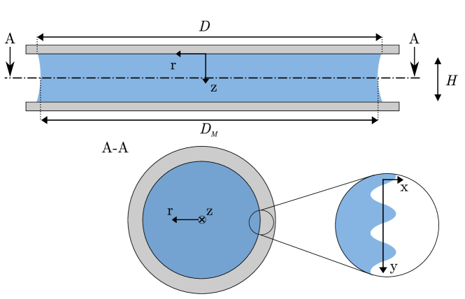
Figure 4: A cylindrical frame of reference is used at the symmetry axis ($r,z$). The area of interest for instability analysis is magnified and a Cartesian frame of reference is used at the interface ($\{x,y\}$).

The experimental setup for stretching a liquid bridge is shown schematically in fig. 1a). The stretching system consists of two substrates orientated horizontally. The lower substrate is mounted on a linear drive which allows accelerations from $10\text{\,}\mathrm{m}\mathrm{/}\mathrm{s}^{2}$ to $180\text{\,}\mathrm{m}\mathrm{/}\mathrm{s}^{2}$. The position accuracy of the linear drive is about $5\text{\,}\mu\mathrm{m}$. The upper substrate is fixed. Both substrates are transparent, fabricated from glass with a roughness of $R_{a}=$80\text{\,}\mathrm{n}\mathrm{m}$$. The initial thickness of the gap, $H_{0}$, in the experiments varies from 20 to 140 $\mu$m, as shown below in fig. 4.

A microliter syringe is used as a fluid dispensing system. To investigate the effect of the liquid properties, two water-glycerol mixtures with different viscosities are used: Gly50 with the viscosity $\mu=5.52\times 10^{-3}$ $\mathrm{Pa}\,\mathrm{s}$, surface tension $\sigma=67.3\times 10^{-3}$ $\text{\,}\mathrm{N}\ \mathrm{m}^{-1}$ and density $\rho=1129.$ $\mathrm{k}\mathrm{g}\ \mathrm{m}^{-3}$; and Gly80 whose properties are $\mu=5.36\times 10^{-2}$ $\mathrm{Pa}\,\mathrm{s}$, $\sigma=65.5\times 10^{-3}$ $\text{\,}\mathrm{N}\ \mathrm{m}^{-1}$ and $\rho=1211.$ $\mathrm{k}\mathrm{g}\ \mathrm{m}^{-3}$. The possible variation of the liquid properties with temperature has been accounted for in the data analysis.

To examine the size effects on the outcome of the liquid bridge stretching, the liquid volumes of the bridge are varied between $1$ and $5\text{\,}\mu\mathrm{l}$. This allows variation of the initial height-to-diameter ratio, $\lambda=H_{0}/D_{0}$, in the range $0.003<\lambda<0.2$.

The observation system consists of two high-speed video systems. The side view camera is equipped with a telecentric lens. The camera on top uses a 12x zoom lens system. The images are captured with a resolution of one megapixel at a frequency of $12.5\text{\,}\mathrm{k}\mathrm{f}\mathrm{p}\mathrm{s}$.

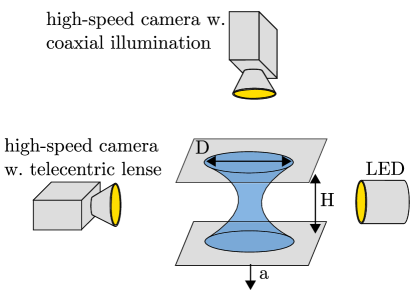
a)              b)

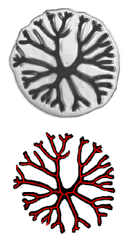
Figure 1: Experimental method: a) the setup and b) post-processing of images.

The post-processing for the top view was performed with the help of trainable weka (arganda-carreras_trainable_2017), a machine learning algorithm assisting with the segmentation of the images. Afterwards the images were skeletonized and the number of fingers was counted. An example of the segmentation and skeleton is shown in fig. 1b) and later in fig. LABEL:fig:functionRR0 the number of fingers is plotted over $R/R_{0}$.

2.2 Observations of the bridge stretching

The experimental setup allows shadowgraphy images of the contact area between the substrate and liquid to be captured during the stretching process. An example of the side-view, high-speed visualization of a stretching $Gly80$ bridge is shown in fig. 2a). In this example the substrate acceleration is $180\text{\,}\mathrm{m}\mathrm{/}\mathrm{s}^{2}$ and the initial height is $20\text{\,}\mu\mathrm{m}$. The initial liquid bridge height-to-diameter ratio is $\lambda=0.02$. While the middle diameter, $D_{M}$, of the bridge reduces during the stretching process, a thin liquid film remains on both substrates. The contact line stays pinned for all performed experiments, evident from the top views from fig. 3. After $12.6\text{\,}\mathrm{m}\mathrm{s}$ the bridge pinches off. In fig. 2b) the evolution of the scaled bridge diameter during stretching is shown as a function of the dimensionless gap width. For the stage when $H\ll D_{M}$ the evolution of the bridge diameter is universal. It does not depend on the substrate acceleration or liquid properties.

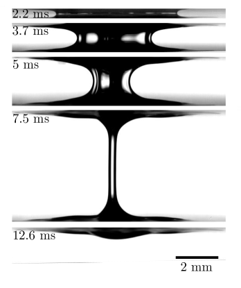
a) b)

Figure 2: Evolution of the diameter of a liquid bridge. (a) Side views of a Gly80 bridge stretched with the constant acceleration $180\text{\,}\mathrm{m}\mathrm{/}\mathrm{s}^{2}$. The initial gap is $20\text{\,}\mu\mathrm{m}$ and the gap-to-diameter ratio is $\lambda=0.02$. (b) The scaled bridge middle diameter $D_{M}/D_{0}$ as a function of the dimensionless gap width $H/H_{0}$ for various substrate accelerations. The curve corresponds to the predictions based on (2).

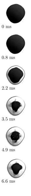
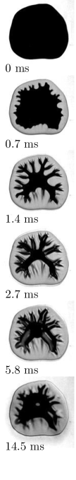
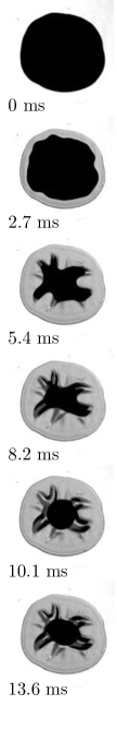
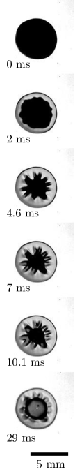
a)	b)	c)	d)

Figure 3: Top view on the receding interface due to the bridge stretching at various experimental conditions. a - liquid $Gly50$, substrate acceleration $a=$ $180\text{\,}\mathrm{m}\mathrm{/}\mathrm{s}^{2}$, relative gap width $\lambda=0.03$; b - $Gly50$, $a=$ $180\text{\,}\mathrm{m}\mathrm{/}\mathrm{s}^{2}$, $\lambda=0.006$; c - $Gly50$, $a=$ $10\text{\,}\mathrm{m}\mathrm{/}\mathrm{s}^{2}$, $\lambda=0.06$; d - $Gly80$, $a=$ $10\text{\,}\mathrm{m}\mathrm{/}\mathrm{s}^{2}$, $\lambda=0.03$.

Several typical top views of the liquid bridge through the transparent substrate are shown in fig. 3 at different instants for various experimental parameters. In some cases the onset of instability can be clearly seen, which leads to the appearance of a net of fingers. The most stable case in fig. 3a corresponds to the relatively wide gap and low acceleration. The most unstable case, associated with the highest number of fingers, corresponds to the highest accelerations and smaller initial gap widths, as in the example fig. 3b. In the example fig. 3c fingers can be observed even with relatively small substrate acceleration, but for small dimensionless heights $\lambda$. Fig. 3d shows how increased liquid viscosity compared to fig. 3 leads to an evolved finger pattern.

Increasing the substrate acceleration or viscosity enhance the fingering instability, whereas with an increasing dimensionless height $\lambda$ the finger formation is mitigated.

3 Stability analysis of the bridge interface

In this study a stability analysis is performed on the basis of experimental measurements of the flow in a thin gap between two substrates. The problem is linearized in the framework of the long-wave approximation.

3.1 Basic flow

The flow field in the stretching liquid bridge can be subdivided into two main regions: meniscus region and the central, inner region, which is not influenced by the meniscus. The solution for an axisymmetric creeping flow between two parallel substrates, one of which moves, is well known (Landau1959). The axial and the radial components of the velocity field are

$$u_{0,r}=-\frac{3\dot{H}rz}{H^{2}}\left(1-\frac{z}{H}\right),\quad u_{0,z}=\frac{3\dot{H}z^{2}}{H^{2}}\left(1-\frac{2z}{3H}\right).$$ (1)

This velocity field satisfies the equation of continuity, the momentum balance equation and the kinematic conditions at both substrates. Unfortunately this solution is not applicable to the case when the effect of the substrate acceleration becomes significant. Moreover, the expression for the velocity field between two substrates (1) is not applicable at the interface of the meniscus. It does not satisfy the conditions for the pressure at the interface, determined by the Young-Laplace equation; and it does not satisfy the conditions of zero shear stress at this interface. Moreover, this velocity field is not able to accurately predict the rate of change of the meniscus radius $\dot{R}$. Let us assume the rate change of the minimum meniscus radius at the middle plane as $\dot{R}=u_{0,r}$ at $z=H/2$. Solution of the equation for the meniscus propagation with the help of (1) yields $R=R_{0}(H_{0}/H)^{3/16}$. This solution does not agree with the experimental data for the evolution of the meniscus radius, therefore the flow in the meniscus region has to be treated differently.

An expression for the radius and the height can be derived from the overall mass balance. Where the initial thickness is $H_{0}$, the initial radius is $R_{0}$ and the lower substrate moves with a constant acceleration $a$. The radius of the bridge $R(t)$ of the bridge meniscus can be estimated as

$$R(t)=R_{0}\left[\frac{H_{0}}{H(t)}\right]^{1/2},\quad H(t)=H_{0}+\frac{at^{2}}{2}$$ (2)

which gives an valid estimate for the initial times when $R(t)\gg H(t)$, as demonstrated on the graph in fig. 2b).

The flow in the meniscus region has to be treated separately. This flow has to satisfy the boundary conditions at the curved meniscus interface and must include also the corner flows (moffatt1964viscous; anderson1993two). The model of the meniscus flow is not trivial and can lead to multiple solutions (gaskell1995modelling). However an accurate solution for the meniscus stability problem has to be based on the meniscus velocity field, since the stresses in this region actually govern the meniscus instability.

In this study we assume that the main reason for the meniscus instability is the appearance of a normal pressure gradient at the meniscus interface. This mechanism is analogous to the Rayleigh-Taylor instability, where the pressure gradient is caused by gravity or by the interface acceleration. This approximate solution is valid only for the case of very small relative gap thickness, $\lambda\ll 1$. Note also, that the ratio of the axial and radial components of the liquid velocity is comparable with $\lambda$. The stresses associated with the axial flow are thus much smaller than those associated with the radial velocity component.

Consider only the dominant terms of the pressure gradient at the interface. The pressure gradient includes the viscous stresses and the inertial terms associated with the material acceleration of the meniscus $\ddot{R}$. The approximation is based on the fact that the radial velocity in the liquid at the interface at the middle plane $(z=H/2)$ is equal to $\dot{R}$. The value of the pressure gradient is then estimated from the Navier-Stokes equations with the help of (2) in the form

$$p_{0,r}=-b\mu\frac{\dot{R}}{H(t)^{2}}-\rho\ddot{R}=\mu atb\frac{\sqrt{H_{0}}R_{0}}{2H^{7/2}}+\rho a\frac{\sqrt{H_{0}}R_{0}}{2H^{5/2}}\left(H_{0}-at^{2}\right),$$ (3)

where $b$ is a dimensionless constant. Its value $b\approx 12$ can be roughly estimated approximating the velocity profile by a parabola, as in the gap-averaged Darcy’s law (shelley_hele_1997; bohr1994viscous; amar_fingering_2005; dias2013wavelength).

Approximation (3) is valid only for the cases of $\lambda\ll 1$ considered in this study. Since the ratio of the axial to the radial velocity, which can be estimated from (2), is comparable with $\lambda$, the effect of the axial velocity on the pressure gradient is negligibly small.

3.2 Planar interface, long-wave approximation of small flow perturbations

Since the radius of the liquid bridge is much larger than the gap thickness, $R\gg H$, the flow leading to small interface disturbances can be considered in a Cartesian coordinate system $\{x,y\}$, where the $x$-coordinate coincides with the radial direction normal to the meniscus, defined as $x=0$, and the $y$-direction is tangential to the meniscus. The coordinate system $\{x,y\}$ is fixed at the meniscus of the liquid bridge, such that

$$r=R(t)+x.$$ (4)

The small flow perturbations in the direction normal to the substrates is neglected. Liquid flow occupies the half-infinite space $x\in]-\infty;\;0]$. Denote $\{u^{\prime}(x,y,t);\;v^{\prime}(x,y,t)\}$ as the velocity vector of the flow perturbations, averaged through the gap width, and $p^{\prime}(x,y,t)$ is the pressure perturbation. The absolute velocity and the pressure $p$ in the gap can be expressed in the form

$$u=\dot{R}(t)+u^{\prime}(x,y,t),\quad v=v^{\prime}(x,y,t),\quad p=p_{0}(x,t)+p^{\prime}(x,y,t).$$ (5)

Therefore, the time derivatives of the components of the velocity field can be written in the form

$$u_{,t}=\ddot{R}+u^{\prime}_{,t}-\dot{R}u^{\prime}_{,x},\quad v_{,t}=v^{\prime}_{,t}-\dot{R}v^{\prime}_{,x}.$$ (6)

The gap thickness $H$ is assumed to be the smallest length scale in the problem. In this case consideration of only the dominant terms in the Navier-Stokes equation, written in the accelerating coordinate system, yields

$$p_{,x} = \mu\left(-b\frac{\dot{R}+u^{\prime}}{H^{2}}+u^{\prime}_{,xx}+u^{\prime}_{,yy}\right)-\rho\ddot{R}-\rho u^{\prime}_{,t},$$ (7a)

$$p_{,y} = \mu\left(-b\frac{v^{\prime}}{H^{2}}+v^{\prime}_{,xx}+v^{\prime}_{,yy}\right)-\rho v^{\prime}_{,t},$$ (7b)

The characteristic value of the leading viscous terms in the pressure gradient expressions (7a) and (7b) is $\mu bu^{\prime}/H_{0}^{2}$. The characteristic time of the problem is $\sqrt{H_{0}/a}$. Therefore, the inertial terms of the flow fluctuations are of order $\rho u^{\prime}_{,t}\sim\rho u^{\prime}\sqrt{a/H_{0}}$. The Reynolds number, defined as the ratio of the inertial and viscous terms, is therefore

$$Re=\frac{a^{1/2}H_{0}^{3/2}\rho}{b\mu}.$$ (8)

In all our experiments the Reynolds number is of order $10^{-2}$. The inertial effects associated with the flow fluctuations are therefore negligibly small. The governing equation for the velocity perturbation can be then obtained from (7a) and (7b) neglecting the terms $\rho u^{\prime}_{,t}$ and $\rho v^{\prime}_{,t}$

$$-b\frac{u^{\prime}_{,y}-v^{\prime}_{,x}}{H^{2}}+u^{\prime}_{,xxy}+u^{\prime}_{,yyy}-v^{\prime}_{,xxx}-v^{\prime}_{,yyx}=0.$$ (9)

The velocity field $\{u^{\prime},v^{\prime}\}$ has to satisfy (9) as well as the continuity equation and the condition of the shear free meniscus surface