Fermion condensation under rotation on
anti-de Sitter space

Abstract

Due to the local curvature, the fermion condensate (FC) for a free Dirac field on anti-de Sitter (adS) space becomes finite, even in the massless limit. Employing the point splitting method using an exact expression for the Feynman two-point function, an experssion for the local FC is derived. Integrating this expression, we report the total FC in the adS volume and on its boundary.

1 Introduction

Over the past couple of decades, the analysis of quantum field theory (QFT) on the anti-de Sitter (adS) background space-time has received much attention due to the conjectured adS/CFT correspondence [1]. Through this conjecture, important insight into the properties of the quark-gluon plasma formed in relativistic heavy-ion collisions was drawn [2].

Recent experiments performed by the STAR collaboration revealed the polarisation of the QGP in non-central collisions [3]. One mechanism that could lead to this polarisation is the chiral vortical effect, due to the spin-orbit coupling predicted through the Dirac equation [4].

In this contribution, we present a study of thermal states of fermions undergoing rigid rotation on the anti-de Sitter space. The focus of this study is the fermion condensate (FC) induced by the coupling to curvature. The discussion is restricted to massless particles in the absence of interaction.

2 Finite temperature expectation values

The line element of adS can be written as:

$$ds^{2}=\frac{1}{\cos^{2}\omega r}\left[-dt^{2}+dr^{2}+\frac{\sin^{2}\omega r}{\omega^{2}}\left(d\theta^{2}+\sin^{2}\theta d\varphi^{2}\right)\right],$$ (1)

where $t\in(-\infty,\infty)$, $0\leq\omega r<\frac{\pi}{2}$ and the inverse radius of curvature $\omega$ is related to the Ricci scalar through $R=-12\omega^{2}$. We further employ the following Cartesian gauge tetrad [5]:

$$e_{{\hat{t}}}= \cos\omega r\,\partial_{t}, e_{{\hat{\imath}}}= \cos\omega r\left[\frac{\omega r}{\sin\omega r}\left(\delta_{ij}-\frac{x^{i}x^{j}}{r^{2}}\right)+\frac{x^{i}x^{j}}{r^{2}}\right]\partial_{j},$$ (2)

by which the local gamma matrices $\gamma^{\mu}=e^{\mu}_{\hat{\alpha}}\gamma^{\hat{\alpha}}$ are written in terms of the Minkowski ones, which satisfy $\{\gamma^{\hat{\alpha}},\gamma^{\hat{\sigma}}\}=-2\eta^{{\hat{\alpha}}{\hat{\sigma}}}$. At finite temperature $\beta_{0}^{-1}$ and in rigid rotation with angular velocity $\bm{\Omega}=\Omega\bm{k}$, we have [6]

$$\braket{\hat{\overline{\Psi}}\hat{\Psi}}_{\beta_{0},\Omega}=\mathcal{Z}^{-1}{\rm tr}(\hat{\rho}\hat{\overline{\Psi}}\hat{\Psi}),\qquad\hat{\rho}=e^{-\beta_{0}(\hat{H}-\Omega\hat{M}^{\hat{z}})},$$ (3)

where $\hat{H}=i\partial_{t}$, $\hat{M}^{\hat{z}}=-i\partial_{\varphi}+S^{\hat{z}}$, $S^{\hat{z}}=\frac{i}{2}\gamma^{\hat{1}}\gamma^{\hat{2}}$ and $\mathcal{Z}={\rm tr}(\hat{\rho})$.

To evaluate Eq. (3), we take the point-splitting approach, by which [7]

$$\braket{\hat{\overline{\Psi}}\hat{\Psi}}_{\beta_{0},\Omega}=-\lim_{x^{\prime}\rightarrow x}{\text{tr}}[iS^{F}_{\beta_{0},\Omega}(x,x^{\prime})\Lambda(x^{\prime},x)],$$ (4)

where $S^{F}_{\beta_{0},\Omega}(x,x^{\prime})$ is the thermal two-point function and $\Lambda(x,x^{\prime})$ is the bispinor of parallel transport, given by [12]:

$$\Lambda(x,x^{\prime})=\frac{\sec(\omega s/2)}{\sqrt{\cos\omega r\cos\omega r^{\prime}}}\Bigg{[}\\ \cos\frac{\omega\Delta t}{2}\left(\cos\frac{\omega r}{2}\cos\frac{\omega r^{\prime}}{2}+\sin\frac{\omega r}{2}\sin\frac{\omega r^{\prime}}{2}\frac{\mathbf{x}\cdot\bm{\gamma}}{r}\frac{\mathbf{x}^{\prime}\cdot\bm{\gamma}}{r^{\prime}}\right)\\ +\sin\frac{\omega\Delta t}{2}\left(\sin\frac{\omega r}{2}\cos\frac{\omega r^{\prime}}{2}\frac{\mathbf{x}\cdot\bm{\gamma}}{r}\gamma^{\hat{t}}+\sin\frac{\omega r^{\prime}}{2}\cos\frac{\omega r}{2}\frac{\mathbf{x}^{\prime}\cdot\bm{\gamma}}{r^{\prime}}\gamma^{\hat{t}}\right)\Bigg{]}.$$ (5)

Using the property $\hat{\rho}\hat{\Psi}(t,\varphi)\hat{\rho}^{-1}=e^{-\beta_{0}\Omega S^{\hat{z}}}\hat{\Psi}(t+i\beta_{0},\varphi+i\beta_{0}\Omega)$, together with the imaginary time anti-periodicity of the two-point function [8], it is possible to compute $S^{F}_{\beta_{0},\Omega}(\Delta t,\Delta\varphi)\equiv S^{F}_{\beta_{0},\Omega}(t,\varphi;t^{\prime},\varphi^{\prime})$ via [9]:

$$S^{F}_{\beta_{0},\Omega}(\Delta t,\Delta\varphi)=\sum_{j=-\infty}^{\infty}(-1)^{j}e^{-j\beta_{0}\Omega S^{\hat{z}}}S^{F}_{\rm vac}(\Delta t+ij\beta_{0},\Delta\varphi+ij\beta_{0}\Omega),$$ (6)

where $S^{F}_{\rm vac}(x,x^{\prime})$ is the vacuum two-point function. The above expression is valid only when the vacua ($\beta_{0}\rightarrow 0$) corresponding to the rotating (fixed $\Omega$) and non-rotating ($\Omega=0$) cases coincide. This is ensured on adS when $|\Omega|\leq\omega$ [10], which we assume to hold for the remainder of this paper.

Due to the maximal symmetry of adS, $S_{\rm vac}^{F}(x,x^{\prime})$ can be written as [11]:

$$iS_{\rm vac}^{F}(x,x^{\prime})=[{\mathcal{A}}(s)+{\mathcal{B}}(s)\not{n}]\Lambda(x,x^{\prime}),$$ (7)

where $n_{\mu}=\nabla_{\mu}s(x,x^{\prime})$ is the normalised tangent at $x$ to the geodesic connecting $x$ and $x^{\prime}$, while the geodesic interval $s$ is given through:

$$\cos\omega s= \frac{\cos\omega\Delta t}{\cos\omega r\cos\omega r^{\prime}}-\cos\gamma\tan\omega r\tan\omega r^{\prime},$$ (8)

where $\gamma$ is the angle between $\bm{x}$ and $\bm{x}^{\prime}$, such that $\cos\gamma=\cos\theta\cos\theta^{\prime}+\sin\theta\sin\theta^{\prime}\cos\Delta\varphi$. For massless fermions, the functions $\mathcal{A}$ and $\mathcal{B}$ are

$${\mathcal{A}}\rfloor_{M=0}=\frac{\omega^{3}}{16\pi^{2}}\left(\cos\frac{\omega s}{2}\right)^{-3},\qquad{\mathcal{B}}\rfloor_{M=0}=\frac{i\omega^{3}}{16\pi^{2}}\left(\sin\frac{\omega s}{2}\right)^{-3}.$$ (9)

3 Analysis and conclusions

Without presenting the details of the computation, we find [10]

$$\braket{:\hat{\overline{\Psi}}\hat{\Psi}:}_{\beta_{0},\Omega}=\sum_{j=1}^{\infty}\frac{(-1)^{j+1}(\cos\omega r)^{4}\cosh\frac{\omega j\beta_{0}}{2}\cosh\frac{\Omega j\beta_{0}}{2}}{2\pi^{2}[\sinh^{2}(\frac{\omega j\beta_{0}}{2})+\cos^{2}\omega r-\sin^{2}\omega r\sin^{2}\theta\sinh^{2}(\frac{\Omega j\beta_{0}}{2})]^{2}}.$$ (10)

The total FC can be obtained by integrating Eq. (10) over the whole space:

$$V^{\rm FC}_{\beta_{0},\Omega}=\int d^{3}x\sqrt{-g}\braket{:\hat{\overline{\Psi}}\hat{\Psi}:}_{\beta_{0},\Omega}=-\sum_{j=1}^{\infty}\frac{(-1)^{j}\cosh(\frac{\Omega j\beta_{0}}{2})/\sinh(\frac{\omega j\beta_{0}}{2})}{\cosh(\omega j\beta_{0})-\cosh(\Omega j\beta_{0})}\\ \simeq\frac{3\zeta(3)T_{0}^{3}}{\omega(\omega^{2}-\Omega^{2})}-\frac{(3\omega^{2}-\Omega^{2})T_{0}}{6\omega(\omega^{2}-\Omega^{2})}\ln 2+O(T_{0}^{-1}).$$ (11)

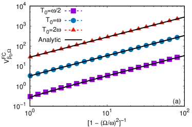
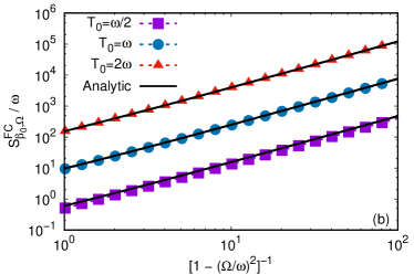
Figure 1: Dependence of (a) $V^{\rm FC}_{\beta_{0},\Omega}$ and (b) $S^{\rm FC}_{\beta_{0},\Omega}/\omega$ with respect to $(1-\Omega^{2}/\omega^{2})^{-1}$, in logarithmic scale. The dotted lines and symbols are numerical results obtained using Eq. (10), while the analytic curves correspond to Eqs. (11) and (12).

On the boundary, the following result is obtained:

$$S^{\rm FC}_{\beta_{0},\Omega}=\int d\Omega\sqrt{-g}\braket{:\hat{\overline{\Psi}}\hat{\Psi}:}_{\beta_{0},\Omega}\\ \simeq\frac{7\pi^{3}T^{4}}{45(\omega^{2}-\Omega^{2})^{3/2}}\left[\frac{\omega}{\Omega}{\rm tan}^{-1}\left(\frac{\Omega/\omega}{\sqrt{1-\frac{\Omega^{2}}{\omega^{2}}}}\right)+\sqrt{1-\frac{\Omega^{2}}{\omega^{2}}}\right]+O(T^{2}).$$ (12)

Both $V^{\rm FC}_{\beta_{0},\Omega}$ (11) and $S^{\rm FC}_{\beta_{0},\Omega}$ are amplified due to the rotation through the prefactors $(1-\Omega^{2}/\omega^{2})^{-1}$ and $(1-\Omega^{2}/\omega^{2})^{-3/2}$, respectively. Figs. 1(a) and 1(b) show the dependence of $V^{\rm FC}_{\beta_{0},\Omega}$ and $S^{\rm FC}_{\beta_{0},\Omega}$ on $(1-\Omega^{2}/\omega^{2})^{-1}$, for various values of the temperature $T_{0}=\beta_{0}^{-1}$. It can be seen that the analytic results (11) and (12) (shown with solid black lines) match well the numerical results (dotted lines and symbols) computed using Eq. (10).

Acknowledgments. This work was supported by a Grant from the Romanian National Authority for Scientific Research and Innovation, CNCS-UEFISCDI, project number PN-III-P1-1.1-PD-2016-1423.

References

• [1] O. Aharony et al., Phys. Rept. 323 (2000) 183–386.
• [2] P. K. Kovtun, D. T. Son, A. O. Starinets, Phys. Rev. Lett. 94 (2005) 111601.
• [3] STAR Collaboration, Nature 548 (2017) 62–65.
• [4] D. E. Kharzeev, J. Liao, S. A. Voloshin, G. Wang, Prog. Part. Nucl. Phys. 88 (2016) 1–28.
• [5] I. I. Cotăescu, Rom. J. Phys. 52 (2007) 895–940.
• [6] A. Vilenkin, Phys. Rev. D 21 (1980) 2260–2269.
• [7] P. B. Groves, P. R. Anderson, E. D. Carlson, Phys. Rev. D 66 (2002) 124017.
• [8] M. Laine, A. Vuorinen, Basics of thermal field theory (Springer, 2016).
• [9] N. D. Birrell, P. C. W. Davies, Quantum fields in curved space (Cambridge University Press, 1982).
• [10] V. E. Ambru\cbs, E. Winstanley, AIP Conf. Proc. 1634 (2014) 40–49.
• [11] W. Mück, J. Phys. A: Math. Gen. 33 (2000) 3021–3026.
• [12] V. E. Ambru\cbs, E. Winstanley, Class. Quant. Grav. 34 (2017) 145010.