Global Helioseismology

Abstract: Helioseismology is one of the most successful fields of astrophysics. The observation and character- ization of solar oscillation has allowed solar seismologists to study the internal structure and dynamics of the Sun with unprecedented thoroughness. Ground-based networks and dedicated space missions have delivered data of exquisite quality, enabling the development of sophisticated inference techniques. The achievements of the fields count, amongst other, the determination of solar photospheric helium abundance, unacessible to spectroscopic constraints, the precise positioning of the base of the convective zone and the demonstration of the importance of microscopic diffusion in stellar radiative regions. Helioseismology played also a key role in validating the framework used to compute solar and stellar models and played an important role in the so-called solar neutrino problem. In the current era of astrophysics, with the increasing importance of asteroseismology to precisely characterize stars, the Sun still plays a crucial calibration role, acting as a benchmark for stellar models. With the revision of the solar abundances and the current discussions related to radiative opacity com- putations, the role of the Sun as a laboratory of fundamental physics is undisputable. In this brief review, I will discuss some of the inference techniques developed in the field of helioseismology, dedicated to the exploitation of the solar global oscillation modes.
Keywords: Helioseismology – Solar Physics – Solar Abundances

1 Introduction

The study of solar oscillations, coined helioseismology by Douglas Gough, has so far been one of the most successful field of astrophysics. Thanks to the excellent quality of the data, the precision of the inferences on the solar structure and the level of details and thoroughness that can be achieved are unmatched in astronomy. Amongst these successes, one can note the precise determination of the position of the base of the convective envelope, the determination of present-day helium abundance, unaccessible to spectroscopy, and the determination of the radial profiles of thermodynamic quantities as well as the 2D rotation velocity profile inside the Sun [82, 27, 144, 61, 84, 43, 4, 5]. These inferences have served to validate the framework of the standard solar models [15, 39, 141], which has since been extensively used to model solar-like stars with asteroseismology. Seismic inference techniques became more and more sophisticated, establishing the reliability of seismology and its position as a “goldgen path” to study stellar structure and evolution. In the meantime, the fundamental ingredients of solar and stellar models were being revised, with improvements made on the equation of state of the solar plasma, the radiative opacities, the transport of chemical elements,… Amongst those revisions, the most problematic one was the reduction of $30\%$ of the solar heavy element abundance by Asplund et al. [12] which led to the so-called “solar modelling problem”. In this paper, I will give a brief overview of the field of global helioseismology, focussing on the inferences from normal acoustic modes using seismic inversion techniques. I will not discuss the field of local helioseismology (see for example [68] for a review on this topic) which focusses on studying the properties of the upper convective zone. I will start in section 2 by a brief history of the observations of solar oscillations and the future of solar missions. I will then discuss the variational approaches for solar rotation and structure inversions and present some results of these inferences in sections 3 and 4. Finally, in section 5, I will briefly discuss how innovative inversion techniques and calibration procedures have been used to gain insights on the solar modelling problem.

2 Observations

The first observations of the solar five minutes oscillation were made by Leighton et al. [89], us- ing Dopplergrams from Mt Wilson Observatory and later confirmed by Evans $\&$ Michard [64]. Detailed analyses of the oscillations by Frazier [66] indicated that the oscillations were not purely superficial, confirming the analysis of P. Mein [92]. Theoretical works by Ulrich [138] and Stein $\&$ Leibacher [129] suggested that the oscillations could be standing acoustic waves. C. Wolff and Ando $\&$ Osaki analysed the stability of such oscillations in the observed frequency and wavenumber range and found that they could be linearly unstable [147, 3]. Their nature was however made clear when F.L. Deubner identified ridges in the wavenumber frequency diagrams [53], confirming the fact that the oscillations were indeed acoustic modes. These observations were independently confirmed by Rhodes et al. [110] who also used them to make inferences on the properties of the solar convective zone.

Quickly, early works were attempted to constrain the properties of the solar interior using the observed oscillation frequencies [119, 41, 79, 114]. Brookes et al. [26] and Servenyi et al. [122] announced the detection of a long period oscillation ($\approx 160min$) in the solar spectrum which was found again later in two independent studies. This long-period signal then disappeared from later observations. The next step was taken by the Claverie et al. [46] and by Grec et al. [74] who provided observations of modes of low harmonic degrees in the same range of period. Both datasets at low and high degrees were bridged by Duvall $\&$ Harvey [58] who observed low and intermediate degree oscillation modes. The stage was thus set for the use of solar seismic observations to constrain solar models (see for example [119, 41, 1, 24, 124] for early works).

In the meantime, observations by Rhodes et al. [111, 54] allowed to determine for the first time the rotational splitting of high degree p modes. The analysis was extended by Duvall et al. [59] on intermediate and low degree modes. These observations were then used to infer the properties of the solar rotation profile (see section 3). With the development of the field, it became clear that long, uninterrupted time-series where required to provide accurate and precise inferences on the solar inter- nal structure. The advent of observational programs such as GONG [77] and BiSON [26, 81], using networks of ground-based observatories provided high-quality data for helioseismic investigations. With the advent of the SOHO spacecraft [56], in 1996, the quality of the data further improved and led to the development and extensive use of sophisticated inversion techniques.

3 Inversions of solar rotation

3.1 Formalism

It is well known from the classical theory of stellar pulsations [38, 139] that for a non-rotating star, the solutions to the eigenvalue problem are degenerate and all the frequencies can be characterised by two quantum numbers only, their degree, $\ell$ and their radial order, $n$. However, if the rotation of the star is taken into account, the symmetry of the system will be broken and the solutions have to be characterised by three quantum numbers, $\ell$, $n$ and the azimuthal order, $m$. In the case of slow rotation, as for the Sun, these effects can be treated as a perturbation of the spherically symmetric solutions and to the first order for a rigid rotation. In that case, the changes on the frequencies are written as

$$\nu^{\pm m}_{n,\ell}=\nu^{0}_{n,\ell}\pm m\beta_{n,\ell}\Omega,$$ (1)

with $\Omega$ the rotation rate of the star, $\nu^{m}_{n,\ell}$, the frequency including the effect of rotation, $\nu^{0}_{n,\ell}$ of the non-rotating star, and $\beta_{n,\ell}$ the Ledoux constant related to rotation. If one considers a differential rotation in radius, the rotational splitting will be symmetrical and one can apply a variational analysis leading to an integral relation between the splitting and the rotational profile. If the horizontal variations of the rotational profile are taken into account, the rotational splitting is not constant anymore. This integral relation was used in the solar case to carry out inversions of the solar rotation profile. In the 2D case, the relation reads

$$\delta\omega_{n,\ell,m}=\frac{m\mathcal{R}_{n,\ell}^{m}}{\int_{0}^{R}\rho_{0}\left[\xi_{r,0}^{2}+\ell(\ell+1)\xi_{h,0}^{2}\right]r^{2}dr},$$ (2)

with $\mathcal{R}^{m}_{n,\ell}$ defined as follows

$$\mathcal{R}_{n,\ell}^{m} =\int_{0}^{\pi}\sin\theta d\theta\int_{0}^{R}\left(|\xi_{r}|^{2}P_{\ell}^{m}(\cos\theta)^{2}+|\xi_{h}|^{2}\left[(\frac{dP_{\ell}^{m}}{d\theta})^{2}+\frac{m^{2}}{\sin^{2}\theta}P_{\ell}^{m}(\cos\theta)^{2}\right]\right.$$ (3)

$$\left.-P_{\ell}^{m}(\cos\theta)^{2}\left[\xi_{r}^{*}\xi_{h}+\xi_{r}\xi_{h}^{*}\right]-2P_{\ell}^{m}(\cos\theta)\frac{dP_{\ell}^{m}}{d\theta}\frac{\cos\theta}{\sin\theta}|\xi_{h}|^{2}\right)\Omega(r,\theta)\rho_{0}(r)r^{2}dr,$$

which is often written in the so-called kernel form

$$\delta\omega_{n,\ell,m}=m\int_{0}^{R}\int_{0}^{\pi}K_{n,\ell,m}(r,\theta)\Omega(r,\theta)rdrd\theta,$$ (4)

with $K^{n,\ell,m}$ the rotational kernel associated with the splitting denoted $\delta\omega_{n,\ell,m}$. A review on the various methods used for rotational inversions can be found in [116]. Other approaches can be used to express the rotational splitting, following a decomposition of the splitted frequencies in a series of Legendre polynomial. We refer the reader to e.g. [117, 101, 38] and references therein for additional discussions of such approaches. In figure 1 we illustrate the behaviour of 1D rotational kernel for various p-modes observed in the solar spectrum and show in Fig 2 the important complementary nature of g-modes to constrain the rotation of the solar core.

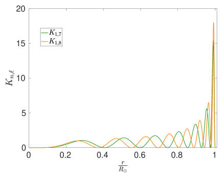
Figure 1: 1D Rotational kernels for low order pressure modes of a standard solar model built using the AGSS09 abundances, FreeEOS equa- tion of state and OPAL opacities.

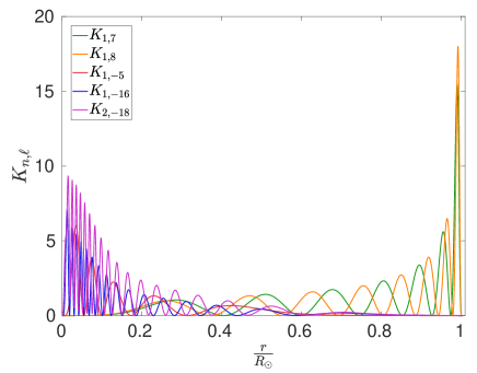
Figure 2: Same as Fig. 1, but also including ro- tational kernels of some gravity modes, showing their capabilities to strongly constrain the rota- tion of the solar core.

The first order approximation is well suited for the Sun which we discuss here, or other typical slow rotators. However, for the sake of completeness, we mention that the first order variational analysis is insufficient for faster rotating stars. One solution is to use high order perturbative develop- ments of the variational approach. It is possible to push further the perturbative developments, lead- ing to higher order expressions (see e.g. [60]). It is also possible to develop fully two-dimensional pulsation codes taking into account the complex geometry of the pulsation modes in fast rotators [107, 106] [105, 108, 98]. Recently, a non-adiabatic version of such a code has been developed [109, 108].

However, the main issue of the fast rotators is the absence of regularity in their oscillation spectra, making it almost impossible to identify the modes.

3.2 Results and current questions

The inversion of the solar rotation profile was first carried out by Brown $\&$ Morrow [27] and by A. Kosovichev [82] and was a striking success for helioseismic inferences. Over the years, the improve- ment of the dataset and of the inversion techniques allowed for a precise 2D cartography of the solar rotation profile. As can be seen from the results of, for example, Schou et al. [117, 116], the rotational inversions are unable to probe the deep core and the poles. This is essentially linked to the behaviour of the kernel functions which are poorly localized in both regions. The low intensity of the kernels in the central regions is a result of the nature of the oscillation, and the same limitations will apply to the structural inversions. Their inability to probe the polar regions results from their asymptotic behaviour with lattitude, falling quickly to 0 at the poles. As a result, even a large number of p modes do not allow to probe efficiently the solar rotation at the poles. The inversion results of the solar rotational profile were a surprise for stellar modellers, as theoretical prescriptions predicted a steep differential rotation in the solar radiative layers. Consequently, the solid-body rotation of the solar radiative zone was a surprise and called for investigations of additional processes for the transport of angular momentum.

A few processes were suggested: fossil fields [36, 72, 127], turbulence-induced gravity waves [37] and the dynamo process suggested by H. Spruit [128, 63]. Recently, plume-induced gravity waves have also been suggested by Pincon et al. [102, 103] to reproduce the core rotation of subgiants observed with Kepler. Hence, as the efficiency of these plume-induced waves has been found to be higher than the ones generated by turbulence, their impact on the rotation profile of solar models should also be tested. Currently, all suggested processes can reproduce with more or less the same degree of agreement the solar rotation profile and thus there is no way to distinguish between them. There has been some debate as to physical occurence of some of these processes in the litterature but none has been currently ruled out.

As a matter of fact, the solution to this issue is linked to the unraveling of the rotation of the solar core. One way to achieve this is by detecting solar gravity modes, which would provide such a diagnostic. In the past, various detections of these modes have been claimed, with the most recent being made by Fossat et al. [65]. However, each detection has been highly debated (see e.g. the work by Schunker et al. [118] and Appourchaux $\&$ Corbard [8] discussing the Fossat et al. detection) and it appears that there is still no undisputed detection of the solar gravity modes. We refer to the paper by Appourchaux et al. [7] for a review on the history of solar g-mode detections.

Besides classical linear inversions, Corbard et al. [49] have also carried non-linear inversions, to resolve the rotation in the tachocline region. Their approach is based on a generalization of the “classical” Regularized Least Square inversion technique used in helioseismology, better known as the Tikohnov regularization. This method uses of a smoothing constraint on the second derivative of the profile of the inverted quantity, which is inadequate to resolve the sharp variations expected in the tachocline. In addition, Corbard et al. [50] attempted to invert the solar core rotation rate from the splitting of low degree p modes but found that the results were not robust and thus could not be used to draw firm conclusions on the solar core rotation rate.

4 Inversions for solar structure

As mentioned above, the detection of the solar oscillations paved the way for the development helioseismic inference techniques. The first comparisons were rather simple and consisted in comparing the frequencies of solar models to the observations. However, it quickly became clear that the small mismatches in frequencies between theoretical models and observations could be used to truly infer the properties of the solar plasma. The first inversions were based on the asymptotic approximation of stellar adiabatic oscillations and used to infer the sound speed profile in the Sun. We will briefly present this approach in Section 4.1. In Section 4.2, we will discuss the variational formalism of structural helioseismic inversions and briefly discuss the variables that can be inverted using these equations as well as the limitations of this formalism.

4.1 Asymptotic inversions

The first solar structural inversions were based on the asymptotic expression of Duvall [57]. The asymptotic analysis of adiabatic oscillations allows to reduce the $4^{th}$ order system to a $2^{nd}$ order one. This is made by using the so-called Cowling approximation, namely that the perturbation to the gravitational potential can be neglected in the pulsation equations.

Interesting properties of oscillations in a specific range of $\ell$ and $n$ can be derived in the asymptotic regime of the stellar oscillations, which drove the first helioseismic inferences and defined helioseis- mology as an inverse problem. A full description of the mathematical developments related to the asymptotic regime of adiabatic stellar oscillations can be found in [123, 135].

Once the Cowling approximation has been used to reduce the order of the system, the equations can be then rewritten (see [71] for a more thorough discussion) as a function of a modified displacement function

$$X =c^{2}\sqrt{\rho}\vec{\nabla}\cdot\vec{\xi}.$$ (5)

By neglecting the variation of the gravity, $g$ and density, $\rho$ when compared to the perturbed thermodynamical quantities, one can obtain a second order differential equation for X

$$\frac{d^{2}X}{dr^{2}} =-K(r)X,$$ (6)

with

$$K(r) =\frac{1}{c^{2}}\left[S^{2}_{\ell}\left(\frac{N^{2}}{\omega^{2}}-1\right)+\omega^{2}-\omega^{2}_{c}\right],$$ (7)

where we defined the acoustic cut-off frequency, $\omega_{c}$ as

$$\omega_{c}^{2} =\frac{c^{2}}{4H_{P}}\left(1-\frac{dH_{P}}{dr}\right).$$ (8)

If $K(r)$ is positive, the solution will be an oscillating function. However, if $K(r)$ is negative, the solution will show an exponential behaviour. In the surface layers, the dominant term of $K(r)$ will be $(\omega^{2}-\omega^{2}_{c})$ because $S^{2}_{\ell}$ becomes negligible. Consequently, the behaviour of the mode will be dictated by the difference $(\omega^{2}-\omega^{2}_{c})$. If $\omega<\omega_{c}$ the mode will show an exponential decay in the upper regions and thus be trapped in the star. If, in contrast, $\omega$ is larger than $\omega_{c}$, it will show an oscillating behaviour in the atmosphere and thus will lose its energy very quickly.

The analytical solution to equation 6 is found by using the JWKB approximation (standing for Jeffreys, Wentzel, Kramers, and Brillouin) which was used in quantum mechanics and applied by Unno et al. [139] in the context of stellar pulsations. The fundamental hypothesis is that the solution will vary faster than the equilibrium quantities. In other words, $X(r)$ varies more rapidly than $K(r)$ and can be described by a function of the form

$$X(r) =a(r)e^{i\phi(r)},$$ (9)

where $\phi(r)$ varies much faster than $a(r)$ and one can derive a local wavelength of the form

$$n =\frac{d\phi}{dr}.$$ (10)

This solution can be inserted in equation 6 and one can find that the behaviour of the solution will again be sinusoidal or exponential depending on the sign of $K(r)$. After some additional mathematical developments and the proper treatment of the boundary conditions at the reflexion points, one can derive the asymptotic form of the eigenfunctions and show that the frequencies of modes trapped between two turning points $r_{1}$ and $r_{2}$ must satisfy the following relation

$$\int_{r_{1}}^{r_{2}}K^{1/2}(r)dr =\left(n-\frac{1}{2}\right)\pi.$$ (11)

For pressure modes which have $\omega^{2}\gg|N|^{2}$, it can be shown that equation 11 reduces to the so-called Duvall law [57]

$$\int_{r_{t}}^{R}\left(1-\frac{(\ell(\ell+1))^{2}c^{2}}{\omega^{2}r^{2}}\right)\frac{dr}{c} =\frac{(n+\alpha(\omega))\pi}{\omega},$$ (12)

with $\alpha(\omega)$ depending on the surface regions, $r_{t}$ being the lower turning point where $S_{\ell}(r_{t})=\omega$ and $R$ the upper turning point where $\omega_{c}(R)=\omega$, which is valid for moderate values of $\ell$.

This expression can then be used to infer the sound speed profile of a solar model. Equation 12 is an integral equation of the Abell type, which can be inverted analytically to infer the sound speed profile. A generalization of this expression for high $\ell$ modes has been derived by Vorontsov $\&$ Shibahashi [145]. In practice, various techniques have been developed to invert the Duvall law [70, 40, 1, 24, 25, 124], with some using a differential formulation of the dispersion relation [44, 43].

4.2 Variational approach

The most commonly used formalism to carry out inversions of the solar structure is based on the variational principle of stellar adiabatic oscillations, which has been derived in a very general context by [35, 91]. The variational formalism can be used to describe the relation between frequency pertur- bations and structural corrections in relatively simple form. This was shown by Dziembowski et al. [62], who wrote the now classical integral relations between frequency perturbations and sound speed and density corrections:

$$\frac{\delta\omega_{n,\ell}}{\omega_{n,\ell}}=\int_{0}^{R}\left[K^{n,\ell}_{c^{2},\rho}\frac{\delta c^{2}}{c^{2}}+K^{n,\ell}_{\rho,c^{2}}\frac{\delta\rho}{\rho}\right]dr,$$ (13)

where we have defined the $K^{n,\ell}_{c^{2},\rho}$, $K^{n,\ell}_{\rho,c^{2}}$, the structural kernels of the $(\rho,c^{2})$ structural pair. It should be noted that these functions are only depending on unperturbed variables, thus only on the theoretical model that is built to carry out the inversion. The mathematical expression of the structural kernels is the following

$$K^{n,\ell}_{c^{2},\rho}=\frac{c^{2}\rho\Lambda^{2}_{\ell}(r)r^{2}}{2E_{n,\ell}\omega_{n,\ell}^{2}},$$ (14)

$$K^{n,\ell}_{\rho,c^{2}}=\frac{1}{2E_{n,\ell}\omega_{n,\ell}^{2}}\left(-\omega^{2}\rho\left[\xi_{r}(r)^{2}+\ell(\ell+1)\xi_{h}(r)^{2}\right]r^{2}+2\rho(\xi_{r}\frac{d\phi^{{}^{\prime}}}{dr}+\frac{\ell(\ell+1)}{r}\xi_{h}\phi^{{}^{\prime}})r^{2}\right.$$

$$-2\xi_{r}\Lambda_{\ell}\rho Gm(r)+4\pi G\rho^{2}\xi_{r}^{2}r^{2}+2\xi_{r}\frac{d\xi_{r}}{dr}G\rho m(r)$$

$$\left.-4\pi\rho G(\int_{r}^{R}\xi_{r}^{2}\frac{d\rho}{dr}+2\Lambda_{\ell}\rho\xi_{r}d\tilde{r})r^{2}+\Lambda_{\ell}^{2}c^{2}\rho r^{2}\right),$$ (15)

where

$$E_{n,\ell}=4\pi\int_{0}^{R}\left[|\tilde{\xi}^{n,\ell}_{r}(r)|^{2}+\ell(\ell+1)|\tilde{\xi}^{n,\ell}_{h}(r)|^{2}\right]\rho r^{2}dr.$$ (16)

This relation has since been extensively exploited to test the internal structure of standard solar models, confirming their good agreement and thus the relative accuracy of our depiction of solar structure.

The variational equations can be modified, implying that one has access to more than the just the sound speed and the density profile of the Sun. This can be done using simple algebra to obtain the kernels related to density and $\Gamma_{1}=\frac{\ln P}{\partial\ln\rho}|_{S}$ perturbations. Other mathematical “tricks” can be used to derive kernels for less obvious structural quantities, such as the Ledoux discriminant or an entropy proxy, defined as $S_{5/3}=\frac{P}{\rho^{5/3}}$ [31, 28]. These methods have been recently used to perform extensive tests of the internal structure of the Sun, in light of the revision of the solar metallicity by Asplund et al. [12]. We illustrate some of the structural kernels used for the inversion of the solar structure in figure 3.

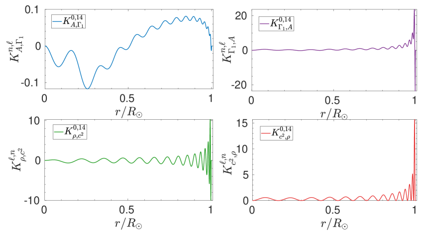
Figure 3: Example of structural kernels for the $(A,\Gamma_{1})$ structural pair (upper figures) and for the $(c^{2},\rho)$ structural pair (lower figures).

As an illustration, we also show in figures 4, 5 and 6 some inversion results for solar models built using both the AGSS09 and GN93 abundances combined with both the OPAL and OPLIB opacities, illustrating the changes that resulted from the revision of the solar opacities. Similar results can be found in LePennec et al. [88] for the OPAS opacities and a more extensive investigation of various inversion results can be found in Buldgen et al. [30]. The dataset used for these inversions is a combination of MDI and BiSON data [19, 51].

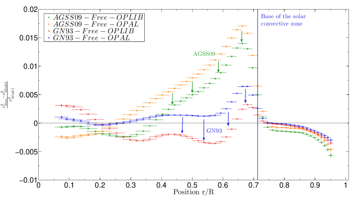
Figure 4: Squared adiabatic sound speed inversions for standard solar models built using the AGSS09 and GN93 abundances combined with both the OPAL and OPLIB opacity tables.

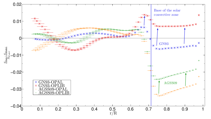
Figure 5: Entropy proxy inversions for standard solar models built using the AGSS09 and GN93 abundances combined with both the OPAL and OPLIB opacity tables.

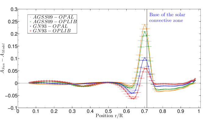
Figure 6: Ledoux discriminant inversions for standard solar models built using the AGSS09 and GN93 abundances combined with both the OPAL and OPLIB opacity tables.

Thanks to these generalized formalisms, any variable that can appear in the adiabatic pulsation equations can be probed using seismic inversions. This enables to focus the seismic information on various aspects of the solar structure. The variational approach can also be extended to derive so- called secondary variables, which do not directly appear in the equations of adiabatic oscillations [73]. Usually, this is done by assuming that the equation of state of the solar plasma is known. Using this approach, one can either directly develop the perturbations of the “acoustic” variables into perturbations of the secondary thermodynamic variables that one wishes to infer, or to fit the inverted results of the “acoustic” variables in the computation of a static solar model (see for example [133, 134, 69, 125]). The variational developments of quantities related to the equation of state have also been used to seismically infer the helium abundance in the convective zone, using perturbations to the adiabatic exponent $\Gamma_{1}$ following the formula

$$\frac{\delta\Gamma_{1}}{\Gamma_{1}}=\frac{\partial\ln\Gamma_{1}}{\partial\ln P}|_{\rho,Y,Z}\frac{\delta P}{P}+\frac{\partial\ln\Gamma_{1}}{\partial\ln\rho}|_{P,Y,Z}\frac{\delta\rho}{\rho}+\frac{\partial\ln\Gamma_{1}}{\partial Y}|_{P,\rho,Z}\delta Y+\frac{\partial\ln\Gamma_{1}}{\partial Z}|_{P,\rho,Y}\delta Z.$$ (17)

with $P$ the pressure, $\rho$ the density, $Y$ the helium and $Z$ the heavy-elements mass fractions. The main weakness of equation 17 is its strong dependency on the equation of state of the solar plasma. This was already noted in early investigations [61, 112], who noted that this was the largest source of uncertainties. Even the recent investigations by Vorontsov and collaborators [142] show relatively large uncertainties in their inferences of the chemical composition of the solar envelope, despite the excellent quality of the seismic data and the thoroughness of the investigation. To circumvent the problem, other authors have used the adimensional sound speed gradient, defined as

$$W(r)=\frac{1}{g}\frac{dc}{dr},$$ (18)

to constrain the helium abundance in the solar envelope, with $g=\frac{Gm}{r^{2}}$. While this quantity is certainly less directly sensitive to the equation of state, the inference still relies on the reproduction of the $\Gamma_{1}$ properties in the helium ionization regions, which are undoubtedly influenced by the properties of the solar equation of state.

Figure 7: Adimensional sound speed gradient as defined by equation 17 for standard solar models built using the AGSS09 abundances, the OPAL opacities and both the FreeEOS and SAHA-S equation of state.

Seismic inversions have also been used to infer constraints on the heavy element abundances in the solar envelope. The first of such an investigation was presented in Takata $\&$ Shibahashi [130], before the revision of the solar abundances. Elliott also investigated the behaviour of $\Gamma_{1}$ to determine the agreement of various equations of state to helioseismic results [64]. They report a good agreement for the GS98 metallicity value but do not attempt to infer it directly from the inverted $\Gamma_{1}$ profile, given its strong dependency in the equation of state. Since then, various groups have made similar attempts, following different approaches. Basu $\&$ Antia attempted to determine the heavy elements abundance in the solar convective region by analysing the behaviour of $W(r)$ and found an abundance in agreement with the GS98 determination [21].

More recently, Vorontsov et al. [142, 143] pointed out the limitations of the study by Antia $\&$ Basu and Basu $\&$ Antia [21, 6], stating that the equation of state they used was not suitable for such detailed investigations. They carried out an extensive study of the properties of the solar convective envelope and determined a low value for the solar metallicity, in agreement with the Asplund value [11, 12]. In 2017, Buldgen et al. [29] carried out an independent study and confirmed the results of Vorontsov et al. [142], noting however the strong dependency on the equation of state and on the properties of the underlying reference model.

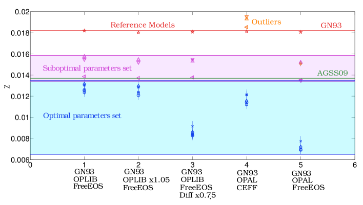
Figure 8: Results of metallicity inversions for various calibrated solar models. The inversion parameters have been changed to analyse the stability of the inversion results (See [29] for more details).

The results of seismic inversions have been used to build so-called seismic solar models [20, 133, 69]. These models do not stem from a standard calibration using evolutionary sequences, but from a reconstruction of the solar structure using helioseismic data assuming hydrostatic and thermal equi- librium. These models have been used to infer the properties of the solar tachocline [134], constrain solar axions [146, 126], but also as “helioseismic” references for comparisons to solar models of various groups.

Given the importance of opacity to infer properties of the solar structure, the variational formal- ism has also been extended to the computation of so-called “opacity kernels” [137], which are use to express the discrepancies of acoustic variables in terms of opacity modifications. These are imple- mented following a perturbative approach, considering a linear response of the structural properties of a model to opacity changes

$$\frac{\delta c}{c}=\int K_{c}(r,T)\delta\log\kappa(T)d\log T,$$ (19)

$$\delta\ln\phi_{\nu}=\int dK_{\phi}(r,T)\delta\log\kappa(T)d\log T.$$ (20)

Examples of these opacity kernels can be found in [140, 141]. The main hypothesis of this approach is that the models will respond linearly to the opacity changes, which is valid within a small range of opacity modifications. Moreover, such variations are static inferences and may not reflect the impact of opacity changes over the whole duration of a solar evolutionary sequence.

Analysing these opacity changes is of particular importance in the context of the solar modelling problem and the potential sources of uncertainties in the Sun that may contribute to the current discrepancies. We will further discuss these points in section 5.

One major difficulty when computing any structural helioseismic inversion is dealing with the so-called surface effects. The issue is well-known in both helio- and asteroseismology and results from the shortcomings of both the computation of solar and stellar oscillations, and that of the stellar models. It is now well-known that the solar pressure modes are generated in the upper parts of the turbulent convective envelope. Hence, the understanding of the driving and damping of the oscillations is intrisically linked to the turbulent closure problem the upper layers of the star, as well as to the non-adiabatic properties of convection, both of which are poorly modelled and understood in stellar conditions.

Thus, the surface effect is often said to arise from both a model and a modal contribution, the former being related to the poor modeling of the properties of the equilibrium structure of the upper parts of convective envelopes and the latter being related to the non-adiabatic properties of the oscillation modes, resulting from the driving and damping by turbulent convection. In nearly all studies of solar-like oscillations, including the Sun, oscillations are computed using the hypothesis of adiabaticity, which is justified in the deep layers of the star only. The variational formalism is no exception, as the hypothesis of adiabaticy is required to derive the symmetry properties of the operator of stellar oscillations, leading in turn to the integral expressions used in the inversions. Furthermore, a few boundary terms of integration by parts are neglected in the derivation of the integral relations between frequency and structure, further contributing to inaccuracies in the surface layers.

The surface effects have been thoroughly studied in the solar case and are most often empirically modelled following a parametrization of the observed trend. From a theoretical point, one can im- pose that the perturbation generated from the surface effects, that we will note $\delta D_{surf}$ , is only of high amplitude in the surface layers. At a given frequency, it is possible to show that the behaviour of the eigenfunctions does not depend on $\ell$ in the surface regions, especially for low degree modes.

As a first approximation, it is assumed that the eigenfunctions do not depend on $\ell$ and this allows to define an equation similar to equation 13 for the surface effect

$$\frac{<\vec{\xi}_{n,\ell},\delta\mathcal{D}_{surf}(\vec{\xi}_{n,\ell})>}{2\omega_{n,\ell}^{2}}=E_{n,\ell}\frac{\delta\omega_{n,\ell}}{\omega_{n,\ell}}.$$ (21)

This equation is formally very similar to equation 13, since we are trying to determine the impact of a perturbation of the model on the frequencies. In this particular case, the perturbation is located in the surface regions and equation 20 will thus behave like the eigenfunctions in these regions. In other words, it will not be strongly dependent on $\ell$, especially if the modes are of low degree. We follow here the developments of Christensen-Dalsgaard [38], introducing a $Q_{n,\ell}$ function defined as

$$Q_{n,\ell}=\frac{E_{n,\ell}}{\bar{E}_{0}(\omega_{n,\ell})},$$ (22)

with $\bar{E}_{0}$ being the inertia of the radial mode at a fixed $\omega$, interpolated in $\omega_{n,\ell}$. One obtains the following relations

$$Q_{n,\ell}\delta\omega_{n,\ell}=\frac{<\vec{\xi}_{n,\ell},\delta\mathcal{D}_{surf}(\vec{\xi}_{n,\ell})>}{2\omega_{n,\ell}\bar{E}_{0}(\omega_{n,\ell})}.$$ (23)

Christensen-Dalsgaard [38] illustrates the effects of this scaling for a comparison between a reference model and a model with a modified opacity in the upper regions. Consequently, this implies that the quantity $Q_{n,\ell}\delta\omega_{n,\ell}$ is largely independent of $\ell$ and, in turn, the surface corrections will also only depend on $\omega$ for a given $\ell$. A first correction is thus to apply this scaling method to eliminate the $\ell$ dependency of the surface effects. However, this scaling is not sufficient to correct the observed biases.

From the analysis of the variational equation 13, we know that no particular care is taken to account for the surface effects. Indeed, the hypotheses of equation 13 are not satisfied in the surface regions and these inaccuracies mean that there is no theoretical expression for $D_{surf}$. Thus, we have to add another function to the integral relations, attempting to take into account surface effects. This function is usually denoted $\mathcal{F}(\omega)$. Using the $Q_{n,\ell}$ factor to normalise the expression, one gets a surface term independent of $\ell$. In fact, $\mathcal{F}(\omega)$ is simply an empirical modelling of the effects of the operator $\delta D_{surf}$ , whose form is unknown. For the $(\rho,c_{2})$ structural pair, one gets the following relation

$$\frac{\delta\omega_{n,\ell}}{\omega_{n,\ell}}=\int_{0}^{R}\left[K^{n,\ell}_{c^{2},\rho}\frac{\delta c^{2}}{c^{2}}+K^{n,\ell}_{\rho,c^{2}}\frac{\delta\rho}{\rho}\right]dr+\frac{\mathcal{F}(\omega)}{Q_{n,\ell}}.$$ (24)

The inversion technique now includes an additional function, taking into account the surface effects that need to be either modelled or eliminated. In practice, it can also be shown that $\mathcal{F}$ must be a slowly varying function of frequency because any sharp variation in the structure leads to an oscillating signature in the frequencies whose frequency is proportional to the acoustic depth of the perturbation. In the case of surface effects, this signature is going to be very slowly varying.

Usually, the $\mathcal{F}$ function is modelled using Legendre polynomials to reproduce the surface effect and including in the inversion technique an additional condition imposing

$$\sum_{i}c_{i}(r_{0})\mathcal{F}(\omega_{i})=0.$$ (25)

This additional condition thus states that the model of the surface effect should be simultaneously cancelled by the inversion as it computes the inversion coefficients used to recombine the frequencies. In practice, the series of Legendre polynomial goes up to order 6 or 7. One should note that there is no physical justification behind the choice of the Legendre polynomials and that one rather speaks of “well chosen functions”.

Another method to model surface effects is to use a low-pass filter on the oscillation data [22]. One then uses an asymptotic form of the relation between frequency and structure, in the form

$$S_{i}\frac{\delta\omega_{i}}{\omega_{i}}\simeq\mathcal{H}_{1}(\frac{\omega_{i}}{L})+\mathcal{H}_{2}(\omega_{i}),$$ (26)

where $L=\ell+1/2$. This expression is derived from the perturbative analysis of the asymptotic relations of pressure modes given in equation 12. The exact analytical expression of the functions $\mathcal{H}_{1}$ and $\mathcal{H}_{2}$ can be found in [42]. The filtering is done in three steps, with the hopes of delivering a correction for the surface effects in the form

$$\sum_{i}a_{i}S_{i}\frac{\delta\omega_{i}}{\omega_{i}}=\mathcal{F}(\omega_{i}).$$ (27)

First, one fits a spline combination to equation 25. This allows to obtain an equation linking frequency corrections to $\mathcal{H}_{2}(\omega)$.

The second step is then to apply a low pass filter to this relation to isolate any slowly varying function of $\omega$. One then obtains a filtered function, $\mathcal{H}_{2}(\omega)$, that is supposed to be linked to $\mathcal{F}(\omega)$.

Thirdly, one fits this filtered $\mathcal{H}_{2}(\omega)$ to obtain a relation similar to equation 26. This fit then allows to define coefficients to correct the individual frequencies such that one eliminates the surface effects based on the asymptotic fit. One should note that due to this correction, the structural kernels are modified and have much lower amplitudes in the surface regions. This method has the disadvantage of introducing correlations between frequency differences, meaning that the treatment of the propagation of errors is also slightly more expensive numerically.

5 The solar modelling problem

Following the revision of the abundances by [11, 10, 9], the helioseismic community was confronted to a significant reduction of the agreement of standard solar models with inverted profiles. The revised abundances were subject to some controversy and various claims stated that they disagreed with helioseismology. Further work by Asplund and collaborators [12] confirmed the revision and thus the “solar metallicity problem”. Caffau and collaborators [32], using different hydrodynamical model than the group of M. Asplund, carried out a re-analysis of solar spectra and found an intermediate value for the solar metallicity. Further investigations were made to determine whether the origin of the discrepancies stemmed from the atmosphere models. These analyses concluded that the small differences in the models could not explain the abundance differences and that the discrepancies between abundance determinations were likely due to the use of different spectral lines, which, in the case of blends [2], could cause an overestimation of the chemical abundances.

The solar problem has since been a tedious issue, as the solution might stem from various con- tributions of constituents of the standard solar model such as the opacities, the equation of state, the computation of microsopic diffusion and the heavy element abundance itself, since it is of course subject to uncertainties. However, the issue has also led modellers to discuss extensively the lim- itations of the standard model framework. For example, the potential of overshooting at the base of the convective zone to reconcile low metallicity models with helioseismic constraint (see e.g. [120, 16, 76, 75, 95, 52, 121]), or scenarios involving accretion of material or intense mass loss in the early days of the solar evolution (see e.g. [34, 148]).

To this days, no clear solution to the solar modelling problem has emerged, despite the publication of updated opacity tables by various groups [94, 48]. In 2015, Bailey and collaborators [17] published results of the first experimental measurements of iron opacity in the physical conditions of the base of the convective envelope. These results led to intense discussions in the opacity community (see e.g. [96, 23, 97, 85, 80, 104]), as the measurements suggested a very significant underestimation of the opacity by theoretical calculations. While theoretical calculations are ongoing [99, 152, 86], it is also important to point out the efforts of independent experimental determinations [113, 78, 100, 33, 47, 55].

Besides the opacity issue, a recent revision of the neon over oxygen ratio from analyses of the solar corona has also been concluded by two independent studies [87, 150]. This revision significantly improves the agreement of AGSS09 models with helioseismic constraints, although not back to the level of agreement of GS98 models.

The main difficulty in trying to constrain the solar modelling problem using helioseismology stems from the fact that seismic analyses do not directly probe key quantities such as the opacity or the mean molecular weight. There will always be some degree of degeneracy in helioseismic inferences, which leads to difficulties in pinpointing the exact causes of the discrepancies. Besides helioseismic inversions, more direct constraints such as the so-called frequency ratios of low-order pressure modes [115] to constrain the properties of the deep radiative layers of solar models. We illustrate in figure 9 the changes that can be observed by changing the opacity tables and chemical abundances of solar models.

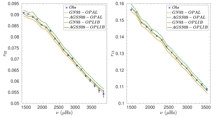
Figure 9: Frequency ratios of low order pressure modes observed by the BIrmingham Solar Oscillation Network compared to standard solar models built using both the GN93 and AGSS09 abundances combined with the OPAL and OPLIB opacities.

An example of such degeneracy is illustrated in Buldgen et al. [30], where combinations of various seismic inversions are used to draw conclusions on the solar modelling problem. Another approach is to use seismic solar models to draw inferences on the properties of other “secondary” thermodynamical quantities as in [125] for example. Other approaches include so-called extended solar calibrations, as discussed in Section 4. These calibrations [13, 14], using more constraints than a classical standard model calibration, allow for the inclusion of “non-standard” corrections to the models, such as modifications of the opacity or the nuclear reaction rates. Interestingly, they draw similar conclusions to the study by Buldgen et al. [30] and other studies using seismic models or ad-hoc corrections to the models. Perhaps one of the most significant conclusion from these studies is that a revision of the opacity on a restricted domain in temperature will not be sufficient to reconcile low metallicity models with helioseismology.

Combining the inferences from seismic solar models with various structural inversions to these calibrations may perhaps provide a way to test with unprecedented thoroughness the ingredients of solar models. For example, helioseismology has clearly proven to be able to probe the temperature and chemical composition gradient just below the base of the convective envelope. Such investigations could provide stringent constraints on the properties of overshooting in stellar envelopes and perhaps a crucial reference point for more realistic prescriptions [149, 109, 151, 67].

6 Conclusion

In this brief review, I have discussed some of the main inference techniques that have been used to exploit the information of the solar global oscillations. More detailed discussions can be found in more extended reviews (e.g. [45, 136, 18, 83]).

It is obvious that the main current issue in the analysis of the global solar oscillations is the inad- equacy between the helioseismic constraints and standard solar models built using the revised solar spectroscopic abundances. While it is certain that these determinations have their own uncertainties, there seems to be no indication that further revisions would reincrease the solar metallicity back to its value inferred from the empirical 1D model. Consequently, the low abundances are here to stay, and it is up to seismologists and modellers to attempt to determine the origin of the discrepancies and reduce them.

In this context, global helioseismology has a strong potential and a bright future. With a tremen- dous amount of data to exploit, a large variety of new methods to implement and exploit, and a strong implication of numerous groups involved in the refinements of the physical ingredients of the solar and stellar models.

However, the stakes of the solar problem are not only a matter of detailed discussions about the solar structure. Indirectly, a revision of the ingredients of solar models will snowball into a revision of the model grids used widely in astrophysics to study all other stars in the Universe and is already leading to intense discussions about the modelling of radiative opacities in stellar conditions. As such, the Sun remains to this day a wonderful laboratory of fundamental physics on both microscopic and macroscopic scales.

References

- [1] Seismology of the Sun and the distant stars. Proceedings of a NATO Advanced Research Workshop, held at Cambridge, UK, 17 - 21 June 1985., volume 169, Jan 1986.
- [2] C. Allende Prieto, D. L. Lambert, and M. Asplund. The Forbidden Abundance of Oxygen in the Sun. ApJL, 556:L63–L66, July 2001.
- [3] H. Ando and Y. Osaki. Nonadiabatic nonradial oscillations: an application to the five-minute oscillation of the sun. PASJ, 27(4):581–603, Jan 1975.
- [4] H. M. Antia and S. Basu. Measuring the helium abundance in the solar envelope: The role of the equation of state. ApJ, 426:801–811, May 1994.
- [5] H. M. Antia and S. Basu. Nonasymptotic helioseismic inversion for solar structure. A&Aps, 107:421–444, November 1994.
- [6] H. M. Antia and Sarbani Basu. Determining Solar Abundances Using Helioseismology. ApJ, 644(2):1292–1298, Jun 2006.
- [7] T. Appourchaux, K. Belkacem, A. M. Broomhall, W. J. Chaplin, D. O. Gough, G. Houdek, J. Provost, F. Baudin, P. Boumier, Y. Elsworth, R. A. García, B. N. Andersen, W. Finsterle, C. Fröhlich, A. Gabriel, G. Grec, A. Jiménez, A. Kosovichev, T. Sekii, T. Toutain, and S. Turck-Chièze. The quest for the solar g modes. A&ARv, 18(1-2):197–277, Feb 2010.
- [8] T. Appourchaux and T. Corbard. Searching for g modes. II. Unconfirmed g-mode detection in the power spectrum of the time series of round-trip travel time. A&Ap, 624:A106, Apr 2019.
- [9] M. Asplund, N. Grevesse, and A. J. Sauval. The Solar Chemical Composition. In T. G. Barnes, III and F. N. Bash, editors, Cosmic Abundances as Records of Stellar Evolution and Nucleosynthesis, volume 336 of Astronomical Society of the Pacific Conference Series, page 25, September 2005.
- [10] M. Asplund, N. Grevesse, A. J. Sauval, C. Allende Prieto, and R. Blomme. Line formation in solar granulation. VI. [C I], C I, CH and C2 lines and the photospheric C abundance. A&Ap, 431:693–705, February 2005.
- [11] M. Asplund, N. Grevesse, A. J. Sauval, C. Allende Prieto, and D. Kiselman. Line formation in solar granulation. IV. [O I], O I and OH lines and the photospheric O abundance. A&Ap, 417:751–768, April 2004.
- [12] M. Asplund, N. Grevesse, A. J. Sauval, and P. Scott. The Chemical Composition of the Sun. ARA&A, 47:481–522, September 2009.
- [13] S. V. Ayukov and V. A. Baturin. A New Approach to the Solar Evolutionary Model with Helioseismic Constraints. In H. Shibahashi and A. E. Lynas-Gray, editors, Progress in Physics of the Sun and Stars: A New Era in Helio- and Asteroseismology, volume 479 of Astronomical Society of the Pacific Conference Series, page 3, Dec 2013.
- [14] S. V. Ayukov and V. A. Baturin. Helioseismic models of the sun with a low heavy element abundance. Astronomy Reports, 61:901–913, October 2017.
- [15] J. N. Bahcall, W. F. Huebner, S. H. Lubow, P. D. Parker, and R. K. Ulrich. Standard solar models and the uncertainties in predicted capture rates of solar neutrinos. Reviews of Modern Physics, 54:767–799, July 1982.
- [16] John N. Bahcall, Sarbani Basu, Marc Pinsonneault, and Aldo M. Serenelli. Helioseismological Implications of Recent Solar Abundance Determinations. ApJ, 618(2):1049–1056, Jan 2005.
- [17] J. E. Bailey, T. Nagayama, G. P. Loisel, G. A. Rochau, C. Blancard, J. Colgan, P. Cossé, G. Faussurier, C. J. Fontes, F. Gilleron, I. Golovkin, S. B. Hansen, C. A. Iglesias, D. P. Kilcrease, J. J. MacFarlane, R. C. Mancini, S. N. Nahar, C. Orban, J. C. Pain, A. K. Pradhan, M. Sherrill, and B. G. Wilson. A higher-than-predicted measurement of iron opacity at solar interior temperatures. Nature, 517:3, January 2015.
- [18] S. Basu and H. M. Antia. Helioseismology and solar abundances. Physics Reports, 457:217–283, March 2008.
- [19] S. Basu, W. J. Chaplin, Y. Elsworth, R. New, and A. M. Serenelli. Fresh Insights on the Structure of the Solar Core. ApJ, 699:1403–1417, July 2009.
- [20] S. Basu and M. J. Thompson. On constructing seismic models of the Sun. A&Ap, 305:631, Jan 1996.
- [21] Sarbani Basu and H. M. Antia. Constraining Solar Abundances Using Helioseismology. ApJL, 606(1):L85–L88, May 2004.
- [22] Sarbani Basu, J. Christensen-Dalsgaard, F. Perez Hernand ez, and M. J. Thompson. Filtering out near-surface uncertainties from helioseismic inversions. MNRAS, 280:651, May 1996.
- [23] C. Blancard, J. Colgan, P. Cossé, G. Faussurier, C. J. Fontes, F. Gilleron, I. Golovkin, S. B. Hansen, C. A. Iglesias, D. P. Kilcrease, J. J. MacFarlane, R. M. More, J.-C. Pain, M. Sherrill, and B. G. Wilson. Comment on “Large Enhancement in High-Energy Photoionization of Fe XVII and Missing Continuum Plasma Opacity”. Physical Review Letters, 117(24):249501, December 2016.
- [24] M. A. Brodskii and S. V. Vorontsov. An Asymptotic Technique for Solving the Inverse Problem of Helioseismology. Soviet Astronomy Letters, 13:179, May 1987.
- [25] M. A. Brodsky and S. V. Vorontsov. On the Technique of the Inversion of Helioseismological Data. In Jorgen Christensen-Dalsgaard and Soren Frandsen, editors, Advances in Helio- and Asteroseismology, volume 123 of IAU Symposium, page 137, Jan 1988.
- [26] J. R. Brookes, G. R. Isaak, and H. B. van der Raay. A resonant-scattering solar spectrometer. MNRAS, 185:1–18, Oct 1978.
- [27] T. M. Brown and C. A. Morrow. Observations of solar p-mode rotational splittings. In B. R. Durney and S. Sofia, editors, The Internal Solar Angular Velocity, volume 137 of Astrophysics and Space Science Library, pages 7–17, 1987.
- [28] G. Buldgen, S. J. A. J. Salmon, M. Godart, A. Noels, R. Scuflaire, M. A. Dupret, D. R. Reese, J. Colgan, C. J. Fontes, P. Eggenberger, P. Hakel, D. P. Kilcrease, and O. Richard. Inversions of the Ledoux discriminant: a closer look at the tachocline. MNRAS, 472:L70–L74, November 2017.
- [29] G. Buldgen, S. J. A. J. Salmon, A. Noels, R. Scuflaire, M. A. Dupret, and D. R. Reese. Determining the metallicity of the solar envelope using seismic inversion techniques. MNRAS, 472:751–764, November 2017.
- [30] G. Buldgen, S. J. A. J. Salmon, A. Noels, R. Scuflaire, J. Montalban, V. A. Baturin, P. Eggenberger, V. K. Gryaznov, I. L. Iosilevskiy, G. Meynet, W. J. Chaplin, A. Miglio, A. V. Oreshina, O. Richard, and A. N. Starostin. Combining multiple structural inversions to constrain the solar modelling problem. A&Ap, 621:A33, Jan 2019.
- [31] G. Buldgen, S. J. A. J. Salmon, A. Noels, R. Scuflaire, D. R. Reese, M.-A. Dupret, J. Colgan, C. J. Fontes, P. Eggenberger, P. Hakel, D. P. Kilcrease, and S. Turck-Chièze. Seismic inversion of the solar entropy. A case for improving the standard solar model. A&Ap, 607:A58, November 2017.
- [32] E. Caffau, H.-G. Ludwig, M. Steffen, B. Freytag, and P. Bonifacio. Solar Chemical Abundances Determined with a CO5BOLD 3D Model Atmosphere. Sol. Phys., 268:255–269, February 2011.
- [33] T. Cardenas, D. W. Schmidt, E. S. Dodd, T. S. Perry, D. Capelli, T. Quintana, J. A. Oertel, Dominic Peterson, E. Giraldez, and R. F. Heeter. Design and fabrication of opacity targets for the national ignition facility. Fusion Science and Technology, 73(3):458–466, 2018.
- [34] M. Castro, S. Vauclair, and O. Richard. Low abundances of heavy elements in the solar outer layers: comparisons of solar models with helioseismic inversions. A&Ap, 463(2):755–758, Feb 2007.
- [35] S. Chandrasekhar and Norman R. Lebovitz. Non-Radial Oscillations of Gaseous Masses. ApJ, 140:1517, Nov 1964.
- [36] P. Charbonneau and K. B. MacGregor. Angular Momentum Transport in Magnetized Stellar Radiative Zones. II. The Solar Spin-down. ApJ, 417:762, Nov 1993.
- [37] Corinne Charbonnel and Suzanne Talon. Influence of Gravity Waves on the Internal Rotation and Li Abundance of Solar-Type Stars. Science, 309(5744):2189–2191, Sep 2005.
- [38] J. Christensen-Dalsgaard. Lecture Notes on Stellar Oscillations. 2003.
- [39] J. Christensen-Dalsgaard, W. Däppen, S. V. Ajukov, E. R. Anderson, H. M. Antia, S. Basu, V. A. Baturin, G. Berthomieu, B. Chaboyer, S. M. Chitre, A. N. Cox, P. Demarque, J. Donatowicz, W. A. Dziembowski, M. Gabriel, D. O. Gough, D. B. Guenther, J. A. Guzik, J. W. Harvey, F. Hill, G. Houdek, C. A. Iglesias, A. G. Kosovichev, J. W. Leibacher, P. Morel, C. R. Proffitt, J. Provost, J. Reiter, E. J. Rhodes, Jr., F. J. Rogers, I. W. Roxburgh, M. J. Thompson, and R. K. Ulrich. The Current State of Solar Modeling. Science, 272:1286–1292, May 1996.
- [40] J. Christensen-Dalsgaard, Jr. Duvall, T. L., D. O. Gough, J. W. Harvey, and Jr. Rhodes, E. J. Speed of sound in the solar interior. Nature, 315(6018):378–382, May 1985.
- [41] J. Christensen-Dalsgaard and D. O. Gough. Towards a heliological inverse problem. Nature, 259(5539):89–92, Jan 1976.
- [42] J. Christensen-Dalsgaard, D. O. Gough, and F. Perez Hernandez. Stellar disharmony. MNRAS, 235:875–880, Dec 1988.
- [43] J. Christensen-Dalsgaard, D. O. Gough, and M. J. Thompson. The depth of the solar convection zone. ApJ, 378:413–437, September 1991.
- [44] J. Christensen-Dalsgaard, M. J. Thompson, and D. O. Gough. Differential asymptotic sound-speed inversions. MNRAS, 238:481–502, May 1989.
- [45] Jørgen Christensen-Dalsgaard. Helioseismology. Reviews of Modern Physics, 74(4):1073–1129, Nov 2002.
- [46] A. Claverie, G. R. Isaak, C. P. McLeod, H. B. van der Raay, and T. R. Cortes. Solar structure from global studies of the 5-minute oscillation. Nature, 282:591–594, Dec 1979.
- [47] A. Colaitis, J.-E. Ducret, M. Le Pennec, X. Ribeyre, and S. Turck-Chièze. Towards a novel stellar opacity measurement scheme using stability properties of double ablation front structures. Physics of Plasmas, 25(7):072707, 2018.
- [48] J. Colgan, D. P. Kilcrease, N. H. Magee, M. E. Sherrill, J. Abdallah, Jr., P. Hakel, C. J. Fontes, J. A. Guzik, and K. A. Mussack. A New Generation of Los Alamos Opacity Tables. ApJ, 817:116, February 2016.
- [49] T. Corbard, L. Blanc-Féraud, G. Berthomieu, and J. Provost. Non linear regularization for helioseismic inversions. Application for the study of the solar tachocline. A&Ap, 344:696–708, Apr 1999.
- [50] T. Corbard, M. P. Di Mauro, T. Sekii, and GOLF Team. The Solar Internal Rotation from GOLF Splittings. In S. Korzennik, editor, Structure and Dynamics of the Interior of the Sun and Sun-like Stars, volume 418 of ESA Special Publication, page 741, Jan 1998.
- [51] G. R. Davies, A. M. Broomhall, W. J. Chaplin, Y. Elsworth, and S. J. Hale. Low-frequency, low-degree solar p-mode properties from 22 years of Birmingham Solar Oscillations Network data. MNRAS, 439:2025–2032, April 2014.
- [52] Franck Delahaye and M. H. Pinsonneault. The Solar Heavy-Element Abundances. I. Constraints from Stellar Interiors. ApJ, 649(1):529–540, Sep 2006.
- [53] F.-L. Deubner. Observations of low wavenumber nonradial eigenmodes of the sun. A&Ap, 44:371–375, November 1975.
- [54] F. L. Deubner, R. K. Ulrich, and Jr. Rhodes, E. J. Solar p-mode oscillations as a tracer of radial differential rotation. A&Ap, 72(1-2):177–185, Feb 1979.
- [55] E. S. Dodd, B. G. DeVolder, M. E. Martin, N. S. Krasheninnikova, I. L. Tregillis, T. S. Perry, R. F. Heeter, Y. P. Opachich, A. S. Moore, J. L. Kline, H. M. Johns, D. A. Liedahl, T. Cardenas, R. E. Olson, B. H. Wilde, and T. J. Urbatsch. Hohlraum modeling for opacity experiments on the national ignition facility. Physics of Plasmas, 25(6):063301, 2018.
- [56] V. Domingo, B. Fleck, and A. I. Poland. The SOHO Mission: an Overview. Sol.Phys., 162(1-2):1–37, Dec 1995.
- [57] Jr. Duvall, T. L. A dispersion law for solar oscillations. Nature, 300(5889):242–243, Nov 1982.
- [58] Jr. Duvall, T. L. and J. W. Harvey. Observations of solar oscillations of low and intermediate degree. Nature, 302(5903):24–27, Mar 1983.
- [59] Jr. Duvall, T. L., J. W. Harvey, and M. A. Pomerantz. Latitude and depth variation of solar rotation. Nature, 321(6069):500–501, May 1986.
- [60] W. A. Dziembowski and Philip R. Goode. Effects of Differential Rotation on Stellar Oscillations: A Second-Order Theory. ApJ, 394:670, Aug 1992.
- [61] W. A. Dziembowski, A. A. Pamiatnykh, and R. . Sienkiewicz. Helium content in the solar convective envelope from helioseismology. MNRAS, 249:602–605, April 1991.
- [62] W. A. Dziembowski, A. A. Pamyatnykh, and R. Sienkiewicz. Solar model from helioseismology and the neutrino flux problem. MNRAS, 244:542–550, June 1990.
- [63] P. Eggenberger, A. Maeder, and G. Meynet. Stellar evolution with rotation and magnetic fields. IV. The solar rotation profile. A&Ap, 440(1):L9–L12, Sep 2005.
- [64] J. W. Evans and R. Michard. Observational Study of Macroscopic Inhomogeneities in the Solar Atmosphere. III. Vertical Oscillatory Motions in the Solar Photosphere. ApJ, 136:493, Sep 1962.
- [65] E. Fossat, P. Boumier, T. Corbard, J. Provost, D. Salabert, F. X. Schmider, A. H. Gabriel, G. Grec, C. Renaud, J. M. Robillot, T. Roca-Cortés, S. Turck-Chièze, R. K. Ulrich, and M. Lazrek. Asymptotic g modes: Evidence for a rapid rotation of the solar core. A&Ap, 604:A40, Aug 2017.
- [66] Edward N. Frazier. An Observational Study of the Hydrodynamics of the Lower Solar Photosphere. ApJ, 152:557, May 1968.
- [67] M. Gabriel and K. Belkacem. A non-local mixing-length theory able to compute core overshooting. A&Ap, 612:A21, Apr 2018.
- [68] Laurent Gizon, Aaron C. Birch, and Henk C. Spruit. Local Helioseismology: Three-Dimensional Imaging of the Solar Interior. ARA&A, 48:289–338, Sep 2010.
- [69] D. Gough. Helioseismological Determination of the State of the Solar Interior. In SOHO-17. 10 Years of SOHO and Beyond, volume 617 of ESA Special Publication, page 1, Jul 2006.
- [70] D. O. Gough. On the Rotation of the Sun. Philosophical Transactions of the Royal Society of London Series A, 313(1524):27–38, Nov 1984.
- [71] D. O. Gough. Linear adiabatic stellar pulsation. In Astrophysical Fluid Dynamics - Les Houches 1987, pages 399–560, Jan 1993.
- [72] D. O. Gough and M. E. McIntyre. Inevitability of a magnetic field in the Sun’s radiative interior. Nature, 394(6695):755–757, Aug 1998.
- [73] Douglas O. Gough and A. G. Kosovichev. An attempt to understand the stanford p-mode data. In E. J. Rolfe, editor, Seismology of the Sun and Sun-Like Stars, volume 286 of ESA Special Publication, pages 195–201, Dec 1988.
- [74] G. Grec, E. Fossat, and M. Pomerantz. Solar oscillations: full disk observations from the geographic South Pole. Nature, 288(5791):541–544, Dec 1980.
- [75] J. A. Guzik, L. S. Watson, and A. N. Cox. Implications of revised solar abundances for helioseismology. MmSAI, 77:389, Jan 2006.
- [76] Joyce A. Guzik, L. Scott Watson, and Arthur N. Cox. Can Enhanced Diffusion Improve Helioseismic Agreement for Solar Models with Revised Abundances? ApJ, 627(2):1049–1056, Jul 2005.
- [77] J. Harvey, K. Abdel-Gawad, W. Ball, B. Boxum, F. Bull, J. Cole, L. Cole, S. Colley, K. Dowdney, R. Drake, R. Dunn, T. Duvall, D. Farris, A. Green, R. Hartlmeier, J. Harvey, R. Hubbard, P. Jackson, D. Kucera, C. Miller, D. Miller, A. Petri, G. Poczulp, J. Schwitters, J. Simmons, R. Smartt, G. Streander, F. Vaughn, P. Wiborg, and GONG Instrument Development Team. The GONG instrument. In E. J. Rolfe, editor, Seismology of the Sun and Sun-Like Stars, volume 286 of ESA Special Publication, pages 203–208, Dec 1988.
- [78] R. F. Heeter, J. E. Bailey, R. S. Craxton, B. G. DeVolder, E. S. Dodd, E. M. Garcia, E. J. Huffman, C. A. Iglesias, J. A. King, J. L. Kline, and et al. Conceptual design of initial opacity experiments on the national ignition facility. Journal of Plasma Physics, 83(1):595830103, 2017.
- [79] Jr. Iben, I. and J. Mahaffy. On the sun’s acoustical spectrum. ApJL, 209:L39–L43, Oct 1976.
- [80] C. A. Iglesias. Iron-group opacities for B stars. MNRAS, 450:2–9, June 2015.
- [81] G. R. Isaak, C. P. McLeod, P. L. Palle, H. B. van der Raay, and T. Roca Cortes. Solar oscillations as seen in the Na I and K I absorption lines. A&Ap, 208:297–302, Jan 1989.
- [82] A. G. Kosovichev. The Internal Rotation of the Sun from Helioseismological Data. Soviet Astronomy Letters, 14:145, March 1988.
- [83] A. G. Kosovichev. Advances in Global and Local Helioseismology: An Introductory Review. In J.-P. Rozelot and C. Neiner, editors, Lecture Notes in Physics, Berlin Springer Verlag, volume 832 of Lecture Notes in Physics, Berlin Springer Verlag, page 3, 2011.
- [84] A. G. Kosovichev and A. V. Fedorova. Construction of a Seismic Model of the Sun. Sov. Astron., 35:507, October 1991.
- [85] M. Krief, A. Feigel, and D. Gazit. Line Broadening and the Solar Opacity Problem. ApJ, 824(2):98, Jun 2016.
- [86] M. Krief and D. Gazit. STAR: A New STA Code for the Calculation of Solar Opacities. In Workshop on Astrophysical Opacities, volume 515 of Astronomical Society of the Pacific Conference Series, page 63, Aug 2018.
- [87] E. Landi and P. Testa. Neon and Oxygen Abundances and Abundance Ratio in the Solar Corona. ApJ, 800:110, February 2015.
- [88] M. Le Pennec, S. Turck-Chièze, S. Salmon, C. Blancard, P. Cossé, G. Faussurier, and G. Mondet. First New Solar Models with OPAS Opacity Tables. ApJL, 813:L42, November 2015.
- [89] R. B. Leighton, R. W. Noyes, and G. W. Simon. Velocity Fields in the Solar Atmosphere. I. Preliminary Report. ApJ, 135:474, March 1962.
- [90] F. Lignières, B. Georgeot, and J. Ballot. P-modes in rapidly rotating stars: Looking for regular patterns in synthetic asymptotic spectra. Astronomische Nachrichten, 331:1053, Dec 2010.
- [91] D. Lynden-Bell and J. P. Ostriker. On the stability of differentially rotating bodies. MNRAS, 136:293, 1967.
- [92] P. Mein. Champ macroscopique des vitesses dans l’atmosphère solaire d’après les mesures de déplacements des raies de Fraunhofer. Annales d’Astrophysique, 29:153, February 1966.
- [93] Giovanni M. Mirouh, George C. Angelou, Daniel R. Reese, and Guglielmo Costa. Mode classification in fast-rotating stars using a convolutional neural network: model-based regular patterns in Scuti stars. MNRAS, 483(1):L28–L32, Feb 2019.
- [94] G. Mondet, C. Blancard, P. Cossé, and G. Faussurier. Opacity Calculations for Solar Mixtures. ApJs, 220:2, September 2015.
- [95] J. Montalban, A. Miglio, S. Theado, A. Noels, and N. Grevesse. The new solar abundances - Part II: the crisis and possible solutions. Communications in Asteroseismology, 147:80–84, Jan 2006.
- [96] S. N. Nahar and A. K. Pradhan. Large Enhancement in High-Energy Photoionization of Fe XVII and Missing Continuum Plasma Opacity. Physical Review Letters, 116(23):235003, June 2016.
- [97] Sultana N. Nahar and Anil K. Pradhan. Nahar and Pradhan Reply:. Physical Review Letters, 117(24):249502, Dec 2016.
- [98] R. M. Ouazzani, M. A. Dupret, and D. R. Reese. Pulsations of rapidly rotating stars. I. The ACOR numerical code. A&Ap, 547:A75, Nov 2012.
- [99] J.-C. Pain and F. Gilleron. Opacity calculations for stellar astrophysics. arXiv e-prints, January 2019.
- [100] T.S. Perry, R.F. Heeter, Y.P. Opachich, P.W. Ross, J.L. Kline, K.A. Flippo, M.E. Sherrill, E.S. Dodd, B.G. DeVolder, T. Cardenas, T.N. Archuleta, R.S. Craxton, R. Zhang, P.W. McKenty, E.M. Garcia, E.J. Huffman, J.A. King, M.F. Ahmed, J.A. Emig, S.L Ayers, M.A. Barrios, M.J. May, M.B. Schneider, D.A. Liedahl, B.G. Wilson, T.J. Urbatsch, C.A. Iglesias, J.E. Bailey, and G.A. Rochau. Replicating the z iron opacity experiments on the nif. High Energy Density Physics, 23:223 – 227, 2017.
- [101] F. P. Pijpers. Solar rotation inversions and the relationship between a-coefficients and mode splittings. A&Ap, 326:1235–1240, Oct 1997.
- [102] C. Pinçon, K. Belkacem, and M. J. Goupil. Generation of internal gravity waves by penetrative convection. A&Ap, 588:A122, Apr 2016.
- [103] C. Pinçon, K. Belkacem, M. J. Goupil, and J. P. Marques. Can plume-induced internal gravity waves regulate the core rotation of subgiant stars? A&Ap, 605:A31, Sep 2017.
- [104] A. K. Pradhan and S. N. Nahar. Recalculation of Astrophysical Opacities: Overview, Methodology and Atomic Calculations. ArXiv e-prints, January 2018.
- [105] D. R. Reese, F. Lignières, J. Ballot, M. A. Dupret, C. Barban, C. van’t Veer-Menneret, and K. B. MacGregor. Frequency regularities of acoustic modes and multi-colour mode identification in rapidly rotating stars. A&Ap, 601:A130, May 2017.
- [106] D. R. Reese, V. Prat, C. Barban, C. van ’t Veer-Menneret, and K. B. MacGregor. Mode visibilities in rapidly rotating stars. A&Ap, 550:A77, Feb 2013.
- [107] D. R. Reese, V. Prat, C. Barban, C. van’t Veer-Menneret, and K. B. MacGregor. Signatures of rotation in oscillation spectra. In S. Boissier, P. de Laverny, N. Nardetto, R. Samadi, D. Valls-Gabaud, and H. Wozniak, editors, SF2A-2012: Proceedings of the Annual meeting of the French Society of Astronomy and Astrophysics, pages 211–214, Dec 2012.
- [108] Daniel Roy Reese, Marc-Antoine Dupret, and Michel Rieutord. Non-adiabatic pulsations in ESTER models. In European Physical Journal Web of Conferences, volume 160 of European Physical Journal Web of Conferences, page 02007, Oct 2017.
- [109] M. Rempel. Overshoot at the Base of the Solar Convection Zone: A Semianalytical Approach. ApJ, 607:1046–1064, June 2004.
- [110] E. J. Rhodes, Jr., R. K. Ulrich, and G. W. Simon. Observations of nonradial p-mode oscillations on the sun. ApJ, 218:901–919, December 1977.
- [111] Jr. Rhodes, E. J., F. L. Deubner, and R. K. Ulrich. A new technique for measuring solar rotation. ApJ, 227:629–637, Jan 1979.
- [112] O. Richard, W. A. Dziembowski, R. Sienkiewicz, and P. R. Goode. On the accuracy of helioseismic determination of solar helium abundance. A&Ap, 338:756–760, October 1998.
- [113] P. W. Ross, R. F. Heeter, M. F. Ahmed, E. Dodd, E. J. Huffman, D. A. Liedahl, J. A. King, Y. P. Opachich, M. B. Schneider, and T. S. Perry. Design of the opacity spectrometer for opacity measurements at the national ignition facility. Review of Scientific Instruments, 87(11):11D623, 2016.
- [114] C. A. Rouse. On the first twenty modes of radial oscillation of the 1968 non-standard solar model. A&Ap, 55(3):477–480, Mar 1977.
- [115] I. W. Roxburgh and S. V. Vorontsov. The ratio of small to large separations of acoustic oscillations as a diagnostic of the interior of solar-like stars. A&A, 411:215–220, November 2003.
- [116] J. Schou, H. M. Antia, S. Basu, R. S. Bogart, R. I. Bush, S. M. Chitre, J. Christensen-Dalsgaard, M. P. Di Mauro, W. A. Dziembowski, A. Eff-Darwich, D. O. Gough, D. A. Haber, J. T. Hoeksema, R. Howe, S. G. Korzennik, A. G. Kosovichev, R. M. Larsen, F. P. Pijpers, P. H. Scherrer, T. Sekii, T. D. Tarbell, A. M. Title, M. J. Thompson, and J. Toomre. Helioseismic Studies of Differential Rotation in the Solar Envelope by the Solar Oscillations Investigation Using the Michelson Doppler Imager. ApJ, 505:390–417, September 1998.
- [117] J. Schou, J. Christensen-Dalsgaard, and M. J. Thompson. On Comparing Helioseismic Two-dimensional Inversion Methods. ApJ, 433:389, Sep 1994.
- [118] Hannah Schunker, Jesper Schou, Patrick Gaulme, and Laurent Gizon. Fragile Detection of Solar g-Modes by Fossat et al. Sol.Phys., 293(6):95, Jun 2018.
- [119] R. Scuflaire, M. Gabriel, A. Noels, and A. Boury. Oscillatory periods in the sun and theoretical models with or without mixing. A&Ap, 45(1):15–18, Dec 1975.
- [120] A. M. Serenelli, J. N. Bahcall, S. Basu, and M. H. Pinsonneault. Helioseismological Implications of Recent Solar Abundance Determinations. In D. Danesy, editor, SOHO 14 Helio- and Asteroseismology: Towards a Golden Future, volume 559 of ESA Special Publication, page 623, Oct 2004.
- [121] A. M. Serenelli, S. Basu, J. W. Ferguson, and M. Asplund. New Solar Composition: The Problem with Solar Models Revisited. ApJl, 705:L123–L127, November 2009.
- [122] A. B. Severnyi, V. A. Kotov, and T. T. Tsap. Observations of solar pulsations. Nature, 259(5539):87–89, Jan 1976.
- [123] H. Shibahashi. Modal Analysis of Stellar Nonradial Oscillations by an Asymptotic Method. PASJ, 31:87–104, Jan 1979.
- [124] H. Shibahashi and T. Sekii. Sound velocity distribution in the Sun inferred from the asymptotic inversion of p-mode spectra. In E. J. Rolfe, editor, Seismology of the Sun and Sun-Like Stars, volume 286 of ESA Special Publication, pages 471–474, Dec 1988.
- [125] H. Shibahashi and S. Tamura. A seismic solar model with the updated elemental abundances. In Proceedings of SOHO 18/GONG 2006/HELAS I, Beyond the spherical Sun, volume 624 of ESA Special Publication, page 81, Oct 2006.
- [126] Hiromoto Shibahashi and Satoru Watanabe. Constraint on particle physics from helioseismology. In Huguette Sawaya-Lacoste, editor, GONG+ 2002. Local and Global Helioseismology: the Present and Future, volume 517 of ESA Special Publication, pages 29–34, Feb 2003.
- [127] F. Spada, A. C. Lanzafame, and A. F. Lanza. A semi-analytic approach to angular momentum transport in stellar radiative interiors. MNRAS, 404(2):641–660, May 2010.
- [128] H. C. Spruit. Dynamo action by differential rotation in a stably stratified stellar interior. A&Ap, 381:923–932, Jan 2002.
- [129] R. F. Stein and J. Leibacher. Waves in the solar atmosphere. ARA&A, 12:407–435, 1974.
- [130] M. Takata and H. Shibahashi. Solar Metal Abundance Inferred from Helioseismology. In Pål Brekke, Bernhard Fleck, and Joseph B. Gurman, editors, Recent Insights into the Physics of the Sun and Heliosphere: Highlights from SOHO and Other Space Missions, volume 203 of IAU Symposium, page 43, Jan 2001.
- [131] Masao Takata. Asymptotic analysis of dipolar mixed modes of oscillations in red giant stars. PASJ, 68(6):109, Dec 2016.
- [132] Masao Takata. Physical formulation of mixed modes of stellar oscillations. PASJ, 68(6):91, Dec 2016.
- [133] Masao Takata and Hiromoto Shibahashi. Solar Models Based on Helioseismology and the Solar Neutrino Problem. ApJ, 504(2):1035–1050, Sep 1998.
- [134] Masao Takata and Hiromoto Shibahashi. Hydrogen Abundance in the Tachocline Layer of the Sun. PASJ, 55:1015–1023, Oct 2003.
- [135] M. Tassoul. Asymptotic approximations for stellar nonradial pulsations. ApJS, 43:469–490, Aug 1980.
- [136] Michael J. Thompson, Jørgen Christensen-Dalsgaard, Mark S. Miesch, and Juri Toomre. The Internal Rotation of the Sun. ARA&A, 41:599–643, Jan 2003.
- [137] S. C. Tripathy and J. Christensen-Dalsgaard. Opacity effects on the solar interior. I. Solar structure. A&Ap, 337:579–590, September 1998.
- [138] R. K. Ulrich. The Five-Minute Oscillations on the Solar Surface. ApJ, 162:993, December 1970.
- [139] W. Unno, Y. Osaki, H. Ando, H. Saio, and H. Shibahashi. Nonradial oscillations of stars. 1989.
- [140] F. L. Villante. Constraints on the Opacity Profile of the Sun from Helioseismic Observables and Solar Neutrino Flux Measurements. ApJ, 724(1):98–110, Nov 2010.
- [141] N. Vinyoles, A. M. Serenelli, F. L. Villante, S. Basu, J. Bergström, M. C. Gonzalez-Garcia, M. Maltoni, C. Peña-Garay, and N. Song. A New Generation of Standard Solar Models. ApJ, 835:202, February 2017.
- [142] S. V. Vorontsov, V. A. Baturin, S. V. Ayukov, and V. K. Gryaznov. Helioseismic calibration of the equation of state and chemical composition in the solar convective envelope. MNRAS, 430:1636–1652, April 2013.
- [143] S. V. Vorontsov, V. A. Baturin, S. V. Ayukov, and V. K. Gryaznov. Helioseismic measurements in the solar envelope using group velocities of surface waves. MNRAS, 441:3296–3305, July 2014.
- [144] S. V. Vorontsov, V. A. Baturin, and A. A. Pamiatnykh. Seismological measurement of solar helium abundance. Nature, 349:49–51, January 1991.
- [145] Sergei V. Vorontsov and Hiromoto Shibahashi. Asymptotic Inversion of the Solar Oscillation Frequencies: Sound Speed in the Solar Interior. PASJ, 43:739–753, Oct 1991.
- [146] S. Watanabe and H. Shibahashi. The Most Stringent Limit on Solar Axions. In K. Sato and T. Shiromizu, editors, New Trends in Theoretical and Observational Cosmology, page 375, Jan 2002.
- [147] Charles L. Wolff. The Five-Minute Oscillations as Nonradial Pulsations of the Entire Sun. ApJL, 177:L87, Oct 1972.
- [148] Suzannah R. Wood, Katie Mussack, and Joyce A. Guzik. Solar Models with Dynamic Screening and Early Mass Loss Tested by Helioseismic, Astrophysical, and Planetary Constraints. Sol.Phys., 293(7):111, Jul 2018.
- [149] D. R. Xiong and L. Deng. The structure of the solar convective overshooting zone. MNRAS, 327:1137–1144, November 2001.
- [150] P. R. Young. Element Abundance Ratios in the Quiet Sun Transition Region. ApJ, 855:15, March 2018.
- [151] Q. S. Zhang. The Solar Abundance Problem: The Effect of the Turbulent Kinetic Flux on the Solar Envelope Model. ApJL, 787:L28, June 2014.
- [152] L. Zhao, W. Eissner, S. N. Nahar, and A. K. Pradhan. Converged R-Matrix Calculations of the Photoionization of Fexvii in Astrophysical Plasmas: from Convergence to Completeness. In Workshop on Astrophysical Opacities, volume 515 of Astronomical Society of the Pacific Conference Series, page 89, Aug 2018.