Energy-Efficient Cooperative Secure Transmission in Multi-UAV Enabled Wireless Networks

Abstract

This paper investigates a multiple unmanned aerial vehicles (UAVs) enabled cooperative secure transmission scheme in the presence of multiple potential eavesdroppers. Specifically, multiple source UAVs (SUAVs) send confidential information to multiple legitimate ground users and in the meantime multiple jamming UAVs (JUAVs) cooperatively transmit interference signals to multiple eavesdroppers in order to improve the legitimate users’ achievable secrecy rate. By taking into account the limited energy budget of UAV, our goal is to maximize the system secrecy energy efficiency (SEE), namely the achievable secrecy rate per energy consumption unit, by jointly optimizing the UAV trajectory, transmit power and user scheduling under the constraints of UAV mobility as well as the maximum transmit power. The resulting optimization problem is shown to be a non-convex and mixed-integer fractional optimization problem, which is challenging to solve. We decompose the original problem into three sub-problems, and then an efficient iterative algorithm is proposed by leveraging the block coordinate descent and Dinkelbach method in combination with successive convex approximation techniques. Simulation results show that the proposed scheme outperforms the other benchmarks significantly in terms of the system SEE.

I Introduction

Historically, unmanned aerial vehicles (UAVs) are primarily used in military purposes, such as recognition mission, surveillance mission, territory detection and others [1]. The UAVs become more and more multi-functional and are promising for civilian applications due to their flexibility and cost-efficiency for wireless networks deployment [2, 3, 4, 5]. The UAV’s flexible mobility can be exploited to design a trajectory that increases network throughput. In fact, there has been considerable work on the implementation of UAV-enabled wireless communication systems such as UAV-aided relaying, UAV-aided ubiquitous coverage, UAV-aided information dissemination as well as data collection, etc [6, 7, 8, 9, 10, 11, 12, 13, 14, 15]. Among them, the works in [6] and [7] considered that the UAV acted as the mobile relaying to deliver the source data to a destination node. In [8, 9, 10, 11], the UAV-aided wireless coverage problem was taken into account with the goal of either maximizing coverage region or maximizing user experience, i.e., quality of service (QoS). The works in [12, 13, 14, 15] studied the UAV-aided data dissemination and collection problems from the perspective of the common throughput maximization in either downlink or uplink transmission by optimizing UAV trajectory.

Although the UAVs leveraged in wireless communication bring many benefits, e.g., higher throughput, better QoS, lower delay, etc., the UAV-aided wireless communication systems are not safe and are more vulnerable to be wiretapped by the malicious eavesdroppers due to the high probabilistic LoS of air-to-ground (A2G) channel [16, 17, 18]. By far, the research of physical layer security (PLS) transmission in traditional cellular networks has been widely studied based on the design of maximizing the security rate [19, 20, 21, 22, 23, 24, 25]. For example, [24] studied the secrecy rate maximization problem in the presence of multiple eavesdroppers. Simulation results showed that with the help of multiple jammers, the system secrecy rate was significantly improved. In [25], the authors further studied a secure energy efficiency optimization problem in the cognitive radio network under the constraints of the minimum harvested energy at energy receiver and the maximum interference leakage at the primary network. It is worth noting that the transmit sources such as base station and WiFi access point are fixed. However, in the UAV-enabled PLS transmission systems, the UAV can freely adjust its heading for executing the missions. If the UAV flies closer to the eavesdroppers, the confidential information is more susceptible to be encrypted. Therefore, it imposes a new challenge to design UAV-aided secure wireless networks. There have been a few works on the research of the UAV-aided secure wireless networks [26, 27, 28, 29, 30, 31]. Specifically, the work in [26] considered a downlink transmission system where the UAV sent the confidential message to a legitimate ground user in the presence of a malicious ground eavesdropper, and a joint UAV trajectory and transmit power was proposed to maximize the secrecy rate. In [27], the authors considered a UAV-aided mobile relying system to enhance the system’s PLS by jointly optimizing the UAV/source transmit power and UAV trajectory. [28] investigated a UAV-enabled mobile jamming scheme, where a UAV was leveraged to send jamming signal to the potential eavesdropper for maximizing the average secrecy rate. Two UAVs applied in secure transmission systems were investigated in [29, 30], where one UAV intended to send the confidential message and the other UAV sent the jamming signal by jointly optimizing the two UAVs trajectories as well as the transmit power to maximize secrecy rate. The work [31] further considered a worst-case secrecy rate maximization case by assuming that the two UAVs only perfectly know the legitimate ground user while partially know the eavesdropper’s location.

Unfortunately, the sustainability and performance of UAV-enabled communication systems are fundamentally limited by the onboard energy of UAVs[32, 33]. Therefore, the secrecy energy efficiency (SEE) of UAV-enabled communication systems, which defined as the ratio of the secrecy rate to UAV energy consumption measured by bits/Joule, is of paramount importance in practice. In fact, there has considerable work on the study of the SEE in traditional PLS systems [34, 35, 36, 37]. Our work is different from the previous studies, which considered the communication related energy. Note that the UAV communication energy is several orders of magnitude lower than the UAV propulsion energy consumption [33]. Therefore, the design of SEE problem in UAV-enabled networks still remains a new open issue. However, there only one literature paid attention to investigating it. In [38], a UAV is exploited to assist delivering the confidential message from a ground source to a legitimate node in the presence of a potential eavesdropper, in which the goal was to maximize system SEE by jointly optimizing UAV trajectory, transmit power, and communication scheduling. However, work [38] is only limited to relaying, in our paper, the UAVs used as aerial base stations are investigated.

In this paper, we consider a system where multiple source UAVs (SUAVs) cooperatively transmit information to the legitimate ground users in the presence of multiple eavesdroppers. In addition, to improve the system secrecy rate, the multiple jamming UAVs (JUAVs) are leveraged to cooperatively send the jamming signals to the eavesdroppers. The motivation of using multi-UAV lies in the potential cooperative transmission ability to achieve better system performance, such as higher secrecy rate and lower access delay. To enhance the spectrum efficiency, we assume that all the UAVs share the same bandwidth to communicate with the ground legitimate users in the downlink transmission. Thus, the UAVs transmit power should be carefully designed to mitigate the co-channel interference. More importantly, the UAV’s propulsion energy consumption is significantly influenced by its velocity and acceleration. As a result, our goal is to maximize the system SEE by jointly optimizing the UAV trajectory, transmit power, and user scheduling under the constraints of UAV mobility as well as maximum transmit power. Note that the work [30] investigated the system with single SUAV and single JUAV serving multiple legitimate ground users while does not considered the UAV’s propulsion energy consumption. In fact, numerical results have shown that the benefits of proposed scheme compared with one single SUAV and single JUAV case. To the best of our knowledge, there is no existing work to study the energy-efficient cooperative secure transmission in multi-UAV enabled wireless communication systems. The main contributions are summarized as follows.

• We propose an energy-efficient cooperative secure transmission scheme in the multi-UAV enabled wireless communication systems. We take into account maximizing the system secrecy rate and minimizing the UAV propulsion energy consumption, and trade off them by formulating the SEE maximization problem subject to the constraints of UAV mobility as well as maximum transmit power.

• We develop a three-layer iterative algorithm to solve the non-convex and mixed integer fractional optimization problem by using block coordinate descent, Dinkelbach method, and successive convex approximation (SCA) techniques. Specifically, for any given UAV trajectory and transmit power, the user scheduling is optimally solved with low computational complexity. For any given UAV trajectory and user scheduling, we propose an efficient algorithm to optimize the UAV transmit power by using the SCA techniques. For any given user scheduling and transmit power, the UAV trajectory is obtained by applying SCA techniques and Dinkelbach method.

• The multiple SUAVs are used to cooperatively transmit information to the legitimate users, as expected, the achievable rate of UAV systems can be improved by optimizing user scheduling and UAVs transmit power. Moreover, for enhancing the performance of UAV-enabled secure transmission systems, multiple JUAVs are leveraged to transmit the jamming signal to the eavesdroppers.

• Numerical results demonstrate the following conclusions. First, the proposed JUAVs-aided scheme achieves significantly higher secrecy rate compared with no JUAVs-aided scheme. Second, the system SEE does not monotonically increase or decrease with period time $T$, in contrast, the UAV system SEE firstly increases with period time $T$ and then decreases with period time $T$. Third, the proposed scheme outperforms the other benchmarks in terms of SEE.

The rest of this paper is organized as follows. In Section II, we introduce the multi-UAV enabled cooperative secure communication systems and formulate the SEE problem. Section III proposes an efficient iterative algorithm to solve the formulated problem by using the block coordinate descent and Dinkelbach method, as well as SCA techniques. In Section IV, numerical results are presented to illustrate superiority of our scheme. Finally, we conclude the paper in Section V.

Figure 1: An illustration of a multi-UAV enabled cooperative secure system.

II system model and problem formulation

Consider a multiple UAVs-aided downlink secure transmission systems, which consist of a set ${\cal K}_{2}$ of $K_{2}$ legitimate users and a set ${\cal K}_{1}$ of $K_{1}$ eavesdroppers as shown in Fig. 1. Denote a set of $M_{1}$ JUAVs as ${\cal M}_{1}$ and a set of $M_{2}$ SUAVs as ${\cal M}_{2}$. We assume that all the UAVs fly at a fixed altitude $H$, which can be considered as the minimum altitude to avoid collision by the infrastructure obstacles. For simplicity, the collision among UAVs is not considered here since it can be readily extended by adding the minimum security distance constraints as in [13]. In addition, we assume that SUAVs and JUAVs perfectly know the legitimate user and eavesdropper locations by proper information exchange. This paper can be easily extended to the case with imperfect location of the eavesdropper. Since our main focus is to present the proposed scheme based on UAV’s SEE to the reader in an easy-to-access manner, we would like to restrict the current contribution to the location perfectly known case.

For ease of exposition, a Cartesian coordinate system is established with all the dimensions measured in meters. The horizontal coordinates of the legitimate users $k_{2}\in{\cal K}_{2}$ and the eavesdroppers $k_{1}\in{\cal K}_{1}$ are respectively denoted by ${\bf w}_{k_{2}}$ and ${\bf w}_{k_{1}}$. The continuous time $T$ is equally divided into $N$ time slots with duration $\delta$. As such, the horizontal coordinate of the $i$-th UAV’s trajectory, velocity and acceleration over horizon time $T$ can be approximately denoted by $N$-length sequences as $\{{\bf q}_{i}[n]\}$, $\{{\bf v}_{i}[n]\}$ and $\{{\bf a}_{i}[n]\}$, $i\in{\cal M}_{1}\cup{\cal M}_{2},n\in{\cal N}=\{1,2,...,N\}$.

Different from terrestrial communications, the UAV-to-ground channel is more likely to be dominated by LoS link, especially for rural or sub-urban environment. Recent field experiments by Qualcomm have verified that the UAV-to-ground channel is indeed dominated by the LoS link for UAVs flying above a certain altitude [39]. In addition, the LoS of A2G channel model is also one of the considered channel models in the recent 3GPP specification [40]. Therefore, the air-to-ground channel power gain from UAV $i$, $i\in{\cal M}_{1}\cup{\cal M}_{2}$, to any ground user $k$, $k\in{\cal K}_{1}\cup{\cal K}_{2}$, at time slot $n$ can be modeled as [6],[13],[41],

$${h_{k,i}}\left[n\right]=\frac{{{\beta_{0}}}}{{d_{k,i}^{2}\left[n\right]}}=\frac{{{\beta_{0}}}}{{{{\left\|{{\bf{q}}_{i}\left[n\right]-{{\bf{w}}}}_{k}\right\|}^{2}}+{H^{2}}}},$$ (1)

where ${d_{k,i}\left[n\right]}$ denotes the distance between UAV $i$ and ground user $k$ within time slot $n$, $\beta_{0}$ represents the reference channel gain at $d=1\rm{m}$.

II-A Secrecy rate

Define a binary variable $x_{k_{2},m_{2}}$, which stands for that the legitimate user $k_{2}$, $k\in{\cal K}_{2}$, is served by SUAV $m_{2}$, $m_{2}\in{\cal M}_{2}$, within time slot $n$ if $x_{k_{2},m_{2}}=1$, otherwise, $x_{k_{2},m_{2}}=0$. Moreover, we assume that within each time slot $n$, one legitimate user can be at most served by one SUAV, and each SUAV can serve at most one legitimate user. Thus, we have

$$\sum\limits_{{k_{2}}=1}^{{K_{2}}}{{x_{{k_{2}},{m_{2}}}}\left[n\right]}\leq 1,{m_{2}}\in{\cal M}_{2},n\in{\cal N},$$ (2)

$$\sum\limits_{{m_{2}}=1}^{{M_{2}}}{{x_{{k_{2}},{m_{2}}}}\left[n\right]}\leq 1,{k_{2}}\in{\cal K}_{2},,n\in{\cal N},$$ (3)

$${x_{{k_{2}},{m_{2}}}}\left[n\right]\in\left\{{0,1}\right\},\forall{k_{2}},{m_{2}},n\in{\cal N}.$$ (4)

If the legitimate user $k_{2}\in{\cal K}_{2}$ is served by UAV $m_{2}\in{\cal M}_{2}$ at time slot $n\in{\cal N}$, the achievable rate of user $k_{2}$ in $\rm{bps}$ can be expressed as

$${R_{{k_{2}}}}[n]=\sum\limits_{{m_{2}}=1}^{{M_{2}}}{{x_{{k_{2}},{m_{2}}}}\left[n\right]{R_{{k_{2}},{m_{2}}}}\left[n\right]},$$ (5)

where ${R_{{k_{2}},{m_{2}}}}\left[n\right]=B{\log_{2}}\left({1+\frac{{{p_{{m_{2}}}}\left[n\right]{h_{{k_{2}},{m_{2}}}}\left[n\right]}}{{\sum\limits_{i\in{{\cal M}_{2}}\backslash\left\{{{m_{2}}}\right\}\cup{{\cal M}_{1}}}{{p_{i}}\left[n\right]{h_{{k_{2}},i}}\left[n\right]}+{\sigma^{2}}}}}\right)$, $p_{m_{2}}[n]$ denotes the transmit power of SUAV $m_{2}$ at time slot $n$, and $\sigma^{2}$ is the additive Gaussian white noise power.

Similarly, the achievable rate of eavesdropper $k_{1}$ wiretapping the user $k_{2}$ at time slot $n$ is given by

$${R_{{k_{1}}\to{k_{2}}}}[n]=\sum\limits_{{m_{2}}=1}^{{M_{2}}}{{x_{{k_{2}},{m_{2}}}}\left[n\right]{R_{{k_{1}},{m_{2}}}}\left[n\right]},$$ (6)

where ${R_{{k_{1}},{m_{2}}}}\left[n\right]=B{\log_{2}}\left({1+\frac{{{p_{{m_{2}}}}\left[n\right]{h_{{k_{1}},{m_{2}}}}\left[n\right]}}{{\sum\limits_{i\in{{\cal M}_{2}}\backslash\left\{{{m_{2}}}\right\}\cup{{\cal M}_{1}}}{{p_{i}}\left[n\right]{h_{{k_{1}},i}}\left[n\right]}+{\sigma^{2}}}}}\right)$.

Therefore, the worst-case secrecy rate of user $k_{2}\in{\cal K}_{2}$ in the presence of $K_{1}$ eavesdroppers over horizon time $T$ is given by [19], [20]

$$R_{{k_{2}}}^{\sec}={\sum\limits_{n=1}^{N}{\left[{{R_{{k_{2}}}}\left[n\right]-\mathop{\max}\limits_{{k_{1}}\in{{\cal K}_{1}}}{R_{{k_{1}}\to{k_{2}}}}[n]}\right]}^{+}},$$ (7)

where $\left[b\right]^{+}={\rm max}\{b,0\}$.

II-B UAV propulsion energy consumption

Herein, a fixed-wing UAV is employed since its flight endurance is typically much longer than that of the rotary-wing UAV. The total energy consumption of fixed-wing UAV consists of two parts: UAV communication energy and UAV propulsion energy. However, [33] shows that the UAV communication energy consumption is several orders of magnitudes lower than the UAV propulsion energy consumption. Thus, the UAV communication energy consumption can be ignored compared with UAV propulsion energy consumption. Based on [33], the total propulsion energy consumption of UAV $i$ over $T$ is given by

$${E_{i}}=\sum\limits_{n=1}^{N}{\left({{c_{1}}{{\left\|{{{\bf{v}}_{i}}\left[n\right]}\right\|}^{3}}+\frac{{{c_{2}}}}{{\left\|{{{\bf{v}}_{i}}\left[n\right]}\right\|}}\left({1+\frac{{{{\left\|{{{\bf{a}}_{i}}\left[n\right]}\right\|}^{2}}}}{{{g^{2}}}}}\right)}\right)},$$ (8)

where $g$ is the gravitational acceleration with nominal value $9.8{\rm m/s^{2}}$, $c_{1}$ and $c_{2}$ are the constant parameters related to the UAV wing area, air density and UAV’s weight [33].

II-C Problem formulation

Let us define $X=\left\{{{x_{{k_{2}},{m_{2}}}}\left[n\right],\forall{k_{2}},{m_{2}},n}\right\}$, $P=\left\{{{p_{{i}}}\left[n\right],\forall i,n}\right\}$, $Q=\left\{{{{\bf{q}}_{i}}[n],{{\bf{v}}_{i}}[n],{{\bf{a}}_{i}}[n],\forall i,n}\right\}$ and ${\cal N}_{1}=\{0,1,...,N\}$. Mathematically, the problem can be formulated as follows

$$({\rm P})\mathop{\max}\limits_{X,P,Q}\frac{{\sum\limits_{{k_{2}}=1}^{{K_{2}}}{{\sum\limits_{n=1}^{N}{\left[{{R_{{k_{2}}}}\left[n\right]-\mathop{\max}\limits_{{k_{1}}\in{{\cal K}_{1}}}{R_{{k_{1}}\to{k_{2}}}}[n]}\right]}^{+}}}}}{{{E_{{\rm{total}}}}}}$$

$${\rm s.t.}\quad\eqref{scheduling1},\eqref{scheduling2},\eqref{scheduling3},$$ (9)

$$\qquad{{\bf{q}}_{i}}\left[{n+1}\right]={{\bf{q}}_{i}}\left[{n}\right]+{{\bf{v}}_{i}}\left[n\right]\delta+\frac{1}{2}{{\bf{a}}_{i}}\left[n\right]{\delta^{2}},$$

$$\qquad\qquad\qquad\qquad\qquad\qquad n\in{\cal N}_{1},i\in{{\cal M}_{1}}\cup{{\cal M}_{2}},$$ (10)

$$\qquad{{\bf{v}}_{i}}\left[n+1\right]={{\bf{v}}_{i}}\left[n\right]+{{\bf{a}}_{i}}\left[n\right]\delta,n\in{\cal N}_{1},i\in{{\cal M}_{1}}\cup{{\cal M}_{2}},$$ (11)

$$\qquad{{\bf{q}}_{i}}\left[0\right]={{\bf{q}}_{i}}\left[{N+1}\right],i\in{{\cal M}_{1}}\cup{{\cal M}_{2}},$$ (12)

$$\qquad{{\bf{v}}_{i}}\left[0\right]={{\bf{v}}_{i}}\left[{N+1}\right],i\in{{\cal M}_{1}}\cup{{\cal M}_{2}},$$ (13)

$$\qquad\left\|{{{\bf{v}}_{i}}\left[n\right]}\right\|\leq{v_{\max}},n\in{\cal N}_{1},i\in{{\cal M}_{1}}\cup{{\cal M}_{2}},$$ (14)

$$\qquad\left\|{{{\bf{a}}_{i}}\left[n\right]}\right\|\leq{a_{\max}},n\in{\cal N}_{1},i\in{{\cal M}_{1}}\cup{{\cal M}_{2}},$$ (15)

$$\qquad 0\leq{p_{i}}\left[n\right]\leq{P_{\max}},i\in{{\cal M}_{1}}\cup{{\cal M}_{2}},$$ (16)

where ${E_{\rm total}}=\sum\limits_{i\in{{\cal M}_{1}}\cup{{\cal M}_{2}}}{{E_{i}}}$; (10)-(15) denote the UAV trajectory constraints; ${\bf q}_{i}[0]$ and ${\bf q}_{i}[N+1]$ denote the initial location and final location of UAV $i$ ; ${\bf v}_{i}[0]$ and ${\bf v}_{i}[N+1]$ denote the initial velocity and final velocity of UAV $i$; (14), (15), and (16) represent the feasible and boundary constraints of the optimization variables.

III energy efficient algorithm design for multi-UAV secure transmission

The problem $(\rm P)$ is a non-convex and mixed integer fractional optimization problem, which is challenging to solve due to the following reasons. First, the binary variables are involved in objective function and constraints (2)-(4). Second, both numerator and denominator in objective function are non-convex, which lead to a non-convex fractional objective function. With that in mind, we decompose the original problem into three sub-problems, namely user scheduling optimization, UAV transmit power optimization, and UAV trajectory optimization. Then, an efficient iterative algorithm is proposed via alternately optimizing these three sub-problems.

III-A User scheduling optimization

In this subsection, we consider the first sub-problem for optimizing the user scheduling $X$ with given UAV transmit power $P$ and UAV trajectory $Q$. Then, the problem $(\rm P)$ can be simplified as

$$({\rm{P1}})\mathop{\max}\limits_{X,{\Gamma_{{k_{2}}}}\left[n\right]}\sum\limits_{{k_{2}}=1}^{{K_{2}}}{\sum\limits_{n=1}^{N}{{\Gamma_{{k_{2}}}}\left[n\right]}}$$

$${\rm s.t.}~{}\eqref{scheduling1}\text{-}\eqref{scheduling3},$$

$$\qquad{R_{{k_{2}}}}\left[n\right]-\mathop{\max}\limits_{{k_{1}}\in{{\cal K}_{1}}}{R_{{k_{1}}\to{k_{2}}}}[n]\geq{\Gamma_{{k_{2}}}}\left[n\right],n\in{\cal N},k_{2},$$ (17)

where $\Gamma_{k_{2}}[n]$ is the slack variable. It is observed that the problem $(\rm P1)$ is an integer optimization problem, which in general has no efficient algorithm to solve it with low computational complexity. A traditional method is to first relax the binary variables into continuous variables, and then reconstruct the binary solution by using the obtained continuous solution [13]. However, it cannot be guaranteed that the reconstructed binary solution is the optimal solution to problem $(\rm P1)$. In addition, mapping the continuous solution to the optimal binary soltuion is a very challenging task, which has higher computational complexity. In contrast, we can obtain the optimal scheduling to problem $(\rm P1)$ based on the Algorithm 1.

Algorithm 1 Proposed method to solve $({\rm P}1)$

1:  for $k_{2}=1$ to $K_{2}$ do

2:   for $m_{2}=1$ to $M_{2}$ do  if $R_{{k_{2}},{m_{2}}}^{\sec}\left[n\right]<0$   Set $x_{{k_{2}},{m_{2}}}\left[n\right]=0$, $R_{{k_{2}},{m_{2}}}^{\sec}\left[n\right]=0$.  end if

3:   end for

4:  end for

5:  for $k_{2}=1$ to $K_{2}$ do  Step 1: compute $\left\{{{k_{2}},m_{2}^{*}}\right\}=\mathop{\arg\max}\limits_{{m_{2}}}R_{{k_{2}},{m_{2}}}^{\sec}\left[n\right]$, and  set $x_{{k_{2}},{m_{2}}}\left[n\right]=0,{m_{2}}\in{{\cal M}_{2}}\backslash\left\{{m_{2}^{*}}\right\}$.

6:  end for

7:  if $\{R_{{k_{2}},{m_{2}^{*}}}^{\sec}\left[n\right],k_{2}\in{\cal K}_{2}\}==0$  Step 2: set $x_{{k_{2}},{m_{2}^{*}}}\left[n\right]=0$, and remove the $R_{{k_{2}},{m_{2}^{*}}}^{\sec}\left[n\right]$  from the set $\{R_{{k_{2}},{m_{2}^{*}}}^{\sec}\left[n\right],k_{2}\in{\cal K}_{2}\}$.

8:  end if

9:  Define the new set $\{R_{{k_{2}},{m_{2}^{*}}}^{\sec}\left[n\right],k_{2}\in{\cal K}_{2}^{new},m_{2}^{*}\in{\cal M}_{2}^{new}\}$.

10:  if there are more than two same index ${\bar{m}}_{2}^{y}$ in the indexes $\{{\bar{m}}_{2}^{y}\in{\cal M}_{2}^{new}\}$,  Step 3: compute $\left\{{{\bar{k}}_{2}^{y},{\bar{m}}_{2}^{y}}\right\}=\mathop{\arg\max}\limits_{{k_{2}}\in{\cal K}_{{\bar{m}}_{2}^{y}}}R_{{k_{2}},{{\bar{m}}_{2}}^{y}}^{\sec}\left[n\right]$  (${\cal K}_{{\bar{m}}_{2}^{y}}$ is the user set containing ${\bar{m}}_{2}^{y}$). Step 4: set ${x_{{\bar{k}}_{2}^{y},{\bar{m}}_{2}^{y}}}=1$, ${x_{k_{2},{\bar{m}}_{2}^{y}}}=0$ $({k_{2}}\in{{\cal K}_{\bar{m}_{2}^{y}}}\backslash\left\{{\bar{k}_{2}^{y}}\right\})$,  and also remove $R_{k_{2},{\bar{m}}_{2}^{y}}^{\sec}\left[n\right]$ $({k_{2}}\in{{\cal K}_{\bar{m}_{2}^{y}}}\backslash\left\{{\bar{k}_{2}^{y}}\right\})$ from  the set $\{R_{{k_{2}},{m_{2}^{*}}}^{\sec}\left[n\right],k_{2}\in{\cal K}_{2}^{new},m_{2}^{*}\in{\cal M}_{2}^{new}\}$.

11:  end if

12:  Define the new set $\{R_{{{\tilde{k}}_{2}},{{\tilde{m}}_{2}}}^{\sec}\left[n\right],{\tilde{k}}_{2}\in{\cal K}_{2}^{renew},{\tilde{m}}_{2}\in{\cal M}_{2}^{renew}\}$, and set $x_{{\tilde{k}}_{2},{\tilde{m}}_{2}}=1$ for ${\tilde{k}}_{2}\in{\cal K}_{2}^{renew},{\tilde{m}}_{2}\in{\cal M}_{2}^{renew}\}$.

In Algorithm 1, $R_{{k_{2}},{m_{2}}}^{\sec}\left[n\right]={R_{{k_{2},m_{2}}}}\left[n\right]-\mathop{\max}\limits_{{k_{1}}\in{{\cal K}_{1}}}{R_{{k_{1},m_{2}}}}[n]$, $\forall n,k_{2}\in{\cal K}_{2},m_{2}\in{\cal M}_{2}$. Since the problem $({\rm P}1)$ can be split into $N$ parallel sub-problems, thus we can solve it separately. For any given time slot $n$ in the Algorithm 1, step 1 stands for that each legitimate user associated with the SUAV with its local benefits maximization. In fact, step 1 obeys the constraint (3). Step 2 makes sure that the secrecy rate is larger than zero when the user is scheduled. Step 3 and Step 4 complies with the constraint (2).

For the stage 1-4, the computational complexity for this loop is $K_{2}M_{2}$. For the stage 5-6, in each loop, the complexity for selecting the optimal $m_{2}$ that maximizing $R_{{k_{2}},{m_{2}}}^{\sec}\left[n\right]$ is $M_{2}-1$, and thus the computational complexity for the stage 5-6 is $K_{2}(M_{2}-1)$. For the stage 7-8, the computational complexity for the determine statement is $K_{2}$. For the stage 10-11, the computational complexity for checking the same ${\bar{m}}_{2}^{y}$ is $C_{{\bar{m}}_{2}^{y}}N_{{\bar{m}}_{2}^{y}}$, where $C_{{\bar{m}}_{2}^{y}}$ is the number of clusters with each cluster containing more than two same ${\bar{m}}_{2}^{y}$ $({\bar{m}}_{2}^{y}\in{\cal M}_{2}^{new})$, and $N_{{\bar{m}}_{2}^{y}}$ is the cardinality of the corresponding cluster. Note that $C_{{\bar{m}}_{2}^{y}}N_{{\bar{m}}_{2}^{y}}\leq M_{2}$. The total computational complexity for solving $({\rm P}1)$ by using Algorithm 1 is ${\cal O}\left({N\left({2{K_{2}}{M_{2}}+{C_{\bar{m}_{2}^{y}}}{N_{\bar{m}_{2}^{y}}}}\right)}\right)$.

However, for the exhaustive search method, at any time slot $n$, there are ${{\mathbb{P}}\left({{M_{2}},{K_{2}}}\right)}$ scheduling choices ($\mathbb{P}$ is a permutation operator). We compute the objective function results of problem $(\rm P1)$ with these choices (the complexity is ${{\mathbb{P}}\left({{M_{2}},{K_{2}}}\right)}$), and then choose the optimal one that maximize problem $(\rm P1)$ (the complexity is ${{\mathbb{P}}\left({{M_{2}},{K_{2}}}\right)}-1$). Thus, the total computational complexity for solving $({\rm P}1)$ by using exhaustive search method is ${\cal O}\left({N\times\left({2{\mathbb{P}}\left({{M_{2}},{K_{2}}}\right)-1}\right)}\right)\left({{K_{2}}\geq{M_{2}}}\right)$. Obviously, the computational complexity of our proposed method is much lower than the exhaustive search method, especially when $N$, $K_{2}$, and $M_{2}$ are large.

III-B UAV power optimization

In this subsection, we consider the second sub-problem $(\rm P2)$ for optimizing UAV transmit power $P$ with given UAV trajectory $Q$ and user scheduling $X$, which can be written as

$$({\rm P}2)\mathop{\max}\limits_{{P,}{\tau_{{k_{2}}}}\left[n\right],{\gamma_{{k_{2}}}}\left[n\right]}\sum\limits_{{k_{2}}=1}^{{K_{2}}}{\sum\limits_{n=1}^{N}{{\tau_{{k_{2}}}}\left[n\right]}}$$

$${\rm{s}}{\rm{.t}}{\rm{.}}{\kern 1.0pt}{\kern 1.0pt}{\kern 1.0pt}{\kern 1.0pt}{\kern 1.0pt}{\kern 1.0pt}{R_{{k_{2}}}}\left[n\right]-{\gamma_{{k_{2}}}}\left[n\right]\geq{\tau_{{k_{2}}}}\left[n\right],n\in{\cal N},k_{2},$$ (18)

$$\qquad{\gamma_{{k_{2}}}}\left[n\right]\geq{R_{k_{1}\to{k_{2}}}},n\in{\cal N},{k_{1}},k_{2},$$ (19)

$$\qquad 0\leq{p_{i}}\leq{P_{\max}},i\in{{\cal M}_{1}}\cup{{\cal M}_{2}},$$ (20)

where $\tau_{k_{2}}$ and $\gamma_{k_{2}}$ are the auxiliary variables.

Problem $(\rm P2)$ is a non-convex optimization problem owing to the non-convex constraints (18) and (19). To proceed, we resort to leveraging the SCA technique to obtain an efficient approximation solution to problem $(\rm P2)$. First, to tackle the non-convex term ${R}_{k_{2}}[n]$ with respect to (w.r.t.) $p_{i}[n]$ in constraint (18), we apply the SCA technique to transform ${R}_{k_{2}}[n]$ into a convex form. Then, we can rewrite $R_{k_{2},m_{2}}$ as follows

$${R_{{k_{2}},{m_{2}}}}\left[n\right]={{\bar{R}}_{{k_{2}},{m_{2}}}}\left[n\right]-{{\tilde{R}}_{{k_{2}},{m_{2}}}}\left[n\right],{k_{2}}\in{{\cal K}_{2}},$$ (21)

where ${{\bar{R}}_{{k_{2}},{m_{2}}}}\left[n\right]=B{\log_{2}}\left({\sum\limits_{i\in{{\cal M}_{1}}\cup{{\cal M}_{2}}}{{p_{i}}\left[n\right]{h_{{k_{2}},i}}\left[n\right]}+{\sigma^{2}}}\right)$ and ${{\tilde{R}}_{{k_{2}},{m_{2}}}}\left[n\right]=B{\log_{2}}\left({\sum\limits_{i\in{{\cal M}_{2}}\backslash\left\{{{m_{2}}}\right\}\cup{{\cal M}_{1}}}{{p_{i}}\left[n\right]{h_{{k_{2}},i}}\left[n\right]}+{\sigma^{2}}}\right)$. It can be seen from (21) that $R_{k_{2},m_{2}}$ is a difference of two concave functions. To proceed, by defining the set $\{p_{i}^{r}[n]\}$ as the given local point at the $r$-th iteration, we have the following result.

$${{\tilde{R}}_{{k_{2}},{m_{2}}}}\left[n\right]\leq B{\log_{2}}\left({\sum\limits_{i\in{{\cal M}_{2}}\backslash\left\{{{m_{2}}}\right\}\cup{{\cal M}_{1}}}{p_{i}^{r}\left[n\right]{h_{{k_{2}},i}}\left[n\right]}+{\sigma^{2}}}\right)$$

$$+B\sum\limits_{i\in{{\cal M}_{2}}\backslash\left\{{{m_{2}}}\right\}\cup{{\cal M}_{1}}}{\frac{{{h_{{k_{2}},i}}\left[n\right]{{\log}_{2}}\left(e\right)}}{{\sum\limits_{j\in{{\cal M}_{2}}\backslash\left\{{{m_{2}}}\right\}\cup{{\cal M}_{1}}}{p_{j}^{r}\left[n\right]{h_{{k_{2}},j}}\left[n\right]}+{\sigma^{2}}}}}\left({{p_{i}}\left[n\right]-p_{i}^{r}\left[n\right]}\right)\overset{a}{=}\tilde{R}_{{k_{2}},{m_{2}}}^{up}\left[n\right].$$ (22)

Lemma 1

For any given power $\{p_{i}^{r}[n]\}$, the inequality is hold in (22) (at the top of next page).

Proof:

Please refer to Appendix A. ∎

From Lemma 1, we can see that the $\tilde{R}_{k_{2},m_{2}}^{up}[n]$ is linear w.r.t. the power $p_{i}[n]$, which indicates that $\tilde{R}_{k_{2},m_{2}}[n]$ can be replaced by its upper bound $\tilde{R}_{k_{2},m_{2}}^{up}[n]$. Thus, it can be readily verified that the constraint (18) is now convex.

To address the non-convex constraint (19), the SCA technique is still applied. Similarly, for $k_{1}\in{\cal K}_{1}$, we can reexpress $R_{k_{1},m_{2}}[n]$ as

$${R_{{k_{1}},{m_{2}}}}\left[n\right]={{\bar{R}}_{{k_{1}},{m_{2}}}}\left[n\right]-{{\tilde{R}}_{{k_{1}},{m_{2}}}}\left[n\right],{k_{1}}\in{{\cal K}_{1}}$$ (23)

where ${{\bar{R}}_{{k_{1}},{m_{2}}}}\left[n\right]=B{\log_{2}}\left({\sum\limits_{i\in{{\cal M}_{1}}\cup{{\cal M}_{2}}}{{p_{i}}\left[n\right]{h_{{k_{1}},i}}\left[n\right]}+{\sigma^{2}}}\right)$ and ${{\tilde{R}}_{{k_{1}},{m_{2}}}}\left[n\right]=B{\log_{2}}\left({\sum\limits_{i\in{{\cal M}_{2}}\backslash\left\{{{m_{2}}}\right\}\cup{{\cal M}_{1}}}{{p_{i}}\left[n\right]{h_{{k_{1}},i}}\left[n\right]}+{\sigma^{2}}}\right)$. It can be seen that $R_{k_{1},m_{2}}$ is also a difference of two concave function, which brings the following lemma.

Lemma 2

For any given power $\{p_{i}^{r}[n]\}$, the inequality is hold in (24) (at the top of next page).

Proof:

The proof is similar to Lemma 1 and omitted here for simplicity. ∎

$${{\bar{R}}_{{k_{1}},{m_{2}}}}\left[n\right]\leq B{\log_{2}}\left({\sum\limits_{i\in{{\cal M}_{1}}\cup{{\cal M}_{2}}}{{p_{i}^{r}}\left[n\right]{h_{{k_{1}},i}}\left[n\right]}+{\sigma^{2}}}\right)$$

$$+B\sum\limits_{i\in{{\cal M}_{1}}\cup{{\cal M}_{2}}}{\frac{{{h_{{k_{1}},i}}\left[n\right]{{\log}_{2}}\left(e\right)}}{{\sum\limits_{j\in{{\cal M}_{1}}\cup{{\cal M}_{1}}}{p_{j}^{r}\left[n\right]{h_{{k_{1}},j}}\left[n\right]}+{\sigma^{2}}}}}\left({{p_{i}}\left[n\right]-p_{i}^{r}\left[n\right]}\right)\overset{b}{=}\bar{R}_{{k_{1}},{m_{2}}}^{up}\left[n\right].$$ (24)

Therefore, with the given local point $\{p_{i}^{r}[n]\}$ and upper bound results ${\tilde{R}}_{k_{2},m_{2}}^{up}[n]$ and ${\bar{R}}_{k_{1},m_{2}}^{up}[n]$, we have

$$({\rm P}2.1)\mathop{\max}\limits_{{P},{\tau_{{k_{2}}}}\left[n\right],{\gamma_{{k_{2}}}}\left[n\right]}\sum\limits_{{k_{2}}=1}^{{K_{2}}}{\sum\limits_{n=1}^{N}{{\tau_{{k_{2}}}}\left[n\right]}}$$

$${\rm s.t.}~{} \sum\limits_{{m_{2}}=1}^{{M_{2}}}{{x_{{k_{2}},{m_{2}}}}\left[n\right]\left({{{\bar{R}}_{{k_{2}},{m_{2}}}}\left[n\right]-\tilde{R}_{{k_{2}},{m_{2}}}^{up}\left[n\right]}\right)}-{\gamma_{{k_{2}}}}\left[n\right]$$

$$\qquad\qquad\qquad\qquad\qquad\quad\geq{\tau_{{k_{2}}}}\left[n\right],n\in{\cal N},{k_{2}},$$ (25)

$${\gamma_{{k_{2}}}}\left[n\right]\geq\sum\limits_{{m_{2}}=1}^{{M_{2}}}{{x_{{k_{2}},{m_{2}}}}\left[n\right]\left({\bar{R}_{{k_{1}},{m_{2}}}^{up}\left[n\right]-{{\tilde{R}}_{{k_{1}},{m_{2}}}}\left[n\right]}\right)},$$

$$\qquad\qquad\qquad\qquad\qquad\qquad\qquad,n\in{\cal N},{k_{1}},{k_{2}},$$ (26)

$$0\leq{p_{i}}\leq{P_{\max}},i\in{{\cal M}_{1}}\cup{{\cal M}_{2}}.$$ (27)

$({\rm P}2.1)$ is a convex optimization problem, which can be efficiently solved by standard convex techniques. Consequently, problem $({\rm P2})$ can be approximately solved by successively updating the transmit power based on the results obtained from $({\rm P}2.1)$.

III-C UAV trajectory optimization

In this subsection, we consider the third sub-problem of $(\rm P)$ for optimizing UAV trajectory with given transmit power and user scheduling. The SCA technique and Dinkelbach method are used to solve this non-convex sub-problem. Furthermore, the convex form does not obey the disciplined CVX rules [42]. To solve this problem, we equivalently reformulate it into recognized rules without loss of optimality.

For the given UAV transmit power $P$ and user scheduling $X$, the third sub-problem of $(\rm P)$ is simplified as

$$({\rm{P}}3)\mathop{\max}\limits_{\scriptstyle Q,{\Phi_{{k_{2}}[n]}},\hfill\atop\scriptstyle{\varphi_{{k_{2}}}}\left[n\right]\hfill}\frac{{\sum\limits_{{k_{2}}=1}^{{K_{2}}}{\sum\limits_{n=1}^{N}{{\Phi_{{k_{2}}}}\left[n\right]}}}}{{\sum\limits_{i\in{{\cal M}_{1}}\cup{{\cal M}_{2}}}{\sum\limits_{n=1}^{N}{{c_{1}}{{\left\|{{{\bf{v}}_{i}}\left[n\right]}\right\|}^{3}}+\frac{{{c_{2}}}}{{\left\|{{{\bf{v}}_{i}}\left[n\right]}\right\|}}\left({1+\frac{{{{\left\|{{{\bf{a}}_{i}}\left[n\right]}\right\|}^{2}}}}{{{g^{2}}}}}\right)}}}}$$

$${\rm{s}}.{\rm{t}}.~{}\eqref{trajectory1}\text{-}\eqref{trajectory6},$$

$$\qquad{R_{{k_{2}}}}\left[n\right]-{\varphi_{{k_{2}}}}\left[n\right]\geq{\Phi_{{k_{2}}}}\left[n\right],n\in{\cal N},{k_{2}},$$ (28)

$$\qquad{\varphi_{{k_{2}}}}\left[n\right]\geq{R_{{k_{1}}\to{k_{2}}}},n\in{\cal N},{k_{1}},{k_{2}},$$ (29)

where $\Phi_{k_{2}}[n]$ and $\varphi_{k_{2}}$ are the slack variables. Note that the problem $(\rm P3)$ is non-convex due to the following reasons. First, the UAV trajectory $Q$ involved in (28) and (29) leads to a non-convex constraint set. Second, the UAV velocity ${\bf v}_{i}[n]$ and acceleration ${\bf a}_{i}[n]$ are coupled in the objective function. Therefore, it is intractable to directly solve the problem $(\rm P3)$ efficiently. In the following, we apply SCA technique and Dinkelbach method to obtain the UAV trajectory. We first reformulate $(\rm P3)$ by introducing slack variables $\{\mu_{i}[n]\}$ as

$$({\rm{P}}3.1)\mathop{\max}\limits_{\scriptstyle Q,{\Phi_{{k_{2}}}}\left[n\right],\hfill\atop\scriptstyle{\mu_{i}}\left[n\right],{\varphi_{{k_{2}}}}\left[n\right]\hfill}\frac{{\sum\limits_{{k_{2}}=1}^{{K_{2}}}{\sum\limits_{n=1}^{N}{{\Phi_{{k_{2}}}}\left[n\right]}}}}{{\sum\limits_{i\in{{\cal M}_{1}}\cup{{\cal M}_{2}}}{\sum\limits_{n=1}^{N}{{c_{1}}{{\left\|{{{\bf{v}}_{i}}\left[n\right]}\right\|}^{3}}+\frac{{{c_{2}}}}{{{\mu_{i}}\left[n\right]}}+\frac{{{c_{2}}{{\left\|{{{\bf{a}}_{i}}\left[n\right]}\right\|}^{2}}}}{{{\mu_{i}}\left[n\right]{g^{2}}}}}}}}$$

$${\rm s.t.}~{}\eqref{trajectory1}\text{-}\eqref{trajectory6},\eqref{p3const1},\eqref{p3const2},$$

$$\qquad{\mu_{i}}\left[n\right]\geq 0,n\in{\cal N},i\in{{\cal M}_{1}}\cup{{\cal M}_{2}},$$ (30)

$$\qquad{\left\|{{{\bf{v}}_{i}}\left[n\right]}\right\|^{2}}\geq{\mu_{i}}\left[n\right],n\in{\cal N},i\in{{\cal M}_{1}}\cup{{\cal M}_{2}},$$ (31)

It can be verified that at the optimal solution to the problem $(\rm P3.1)$, we must have ${\left\|{{{\bf{v}}_{i}}\left[n\right]}\right\|^{2}}={\mu_{i}}\left[n\right],n\in{\cal N},i\in{{\cal M}_{1}}\cup{{\cal M}_{2}}$, which means the problem $(\rm P3)$ is equivalent to $(\rm P3.1)$. This can be proved by using reduction to absurdity. Suppose that at the optimal value to problem $(\rm P3.1)$, ${\left\|{{{\bf{v}}_{i}}\left[n\right]}\right\|^{2}}>{\mu_{i}}\left[n\right],n\in{\cal N},i\in{{\cal M}_{1}}\cup{{\cal M}_{2}}$, one can always appropriately increase $\mu_{i}[n]$ to obtain a strictly larger objective value, which is contradictory to the assumption. Therefore, problem $(\rm P3.1)$ is equivalent to $(\rm P3)$. Obviously, (31) is a non-convex constraint. By applying the first-order Taylor expansion at local point $v_{i}^{r}[n]$, we have

$${\left\|{{v_{i}}\left[n\right]}\right\|^{2}}\geq {\left\|{v_{i}^{r}\left[n\right]}\right\|^{2}}+2{\left({v_{i}^{r}\left[n\right]}\right)^{T}}\left({{v_{i}}\left[n\right]-v_{i}^{r}\left[n\right]}\right)$$

$$={\Upsilon^{lb}}\left({{v_{i}}\left[n\right]}\right),n\in{\cal N},i\in{{\cal M}_{1}}\cup{{\cal M}_{2}},$$ (32)

Subsequently, the constraint (31) can be rewritten as

$${\Upsilon^{lb}}\left({{v_{i}}\left[n\right]}\right)\geq{\mu_{i}}\left[n\right],n\in{\cal N},i\in{{\cal M}_{1}}\cup{{\cal M}_{2}},$$ (33)

which is convex since ${\Upsilon^{lb}}\left({{v_{i}}\left[n\right]}\right)$ is linear w.r.t. $v_{i}[n]$.

To tackle the non-convex constraint (28), the SAC technique is leveraged. Specifically, by introducing auxiliary variables $\{S_{k_{2},i}[n],n\in{\cal N},k_{2}\in{\cal K}_{2},i\in{\cal M}_{1}\cup{\cal M}_{2}\}$ into ${\tilde{R}}_{k_{2},m_{2}}[n]$ in (21), ${\tilde{R}}_{k_{2},m_{2}}[n]$ can be substituted as

$${{\tilde{\tilde{R}}}_{{k_{2},m_{2}}}}[n]=B{\log_{2}}\left({\sum\limits_{i\in{{\cal M}_{2}}\backslash\left\{{{m_{2}}}\right\}\cup{{\cal M}_{1}}}{\frac{{{p_{i}}\left[n\right]{\beta_{0}}}}{{{H^{2}}+{S_{{k_{2}},i}}\left[n\right]}}}+{\sigma^{2}}}\right),$$

$$\qquad\qquad\qquad\qquad\qquad\qquad\forall{k_{2}},n\in{\cal N},m\in{\cal M}_{2},$$ (34)

with additional constraint

$${S_{{k_{2}},i}}\left[n\right]\leq{\left\|{{{\bf{q}}_{i}}[n]-{{\bf{w}}_{{k_{2}}}}}\right\|^{2}},\forall{k_{2}},n\in{\cal N},i\in{{\cal M}_{2}}\backslash\left\{{{m_{2}}}\right\}\cup{{\cal M}_{1}},$$ (35)

It is observed from (35) that $\|{\bf q}_{i}[n]-{\bf w}_{k_{2}}[n]\|^{2}$ leads to a non-convex constraint set. To handle the non-convexity of (35), we have the following inequality by applying the first-order Taylor expansion at the given local point $\|{\bf q}_{i}^{r}[n]-{\bf w}_{k_{2}}\|$ at $r$-th iteration

$${\left\|{{{\bf{q}}_{i}}[n]-{{\bf{w}}_{{k_{2}}}}}\right\|^{2}}\geq {\left\|{{\bf{q}}_{i}^{r}[n]-{{\bf{w}}_{{k_{2}}}}}\right\|^{2}}+2{\left({{\bf{q}}_{i}^{r}[n]-{{\bf{w}}_{{k_{2}}}}}\right)^{T}}$$

$$\times\left({{{\bf{q}}_{i}}[n]-{\bf{q}}_{i}^{r}[n]}\right)={\chi^{lb}}\left({{{\bf{q}}_{i}}[n]}\right),$$ (36)

which is convex since ${\chi^{lb}}({\bf q}_{i}[n])$ is linear w.r.t. ${\bf q}_{i}[n]$.

Although ${\tilde{\tilde{R}}}$ is convex w.r.t. $S_{k_{2},i}[n]$ in (34), it does not obey the disciplined CVX rules.

Lemma 3

To make the problem $(\rm P3.1)$ efficiently solved by CVX, (34) can be transformed into

$${{\tilde{\tilde{\tilde{R}}}}_{{k_{2},m_{2}}}}[n]=B\varpi[n],$$ (37)

with additional constraints

$$\left\{\begin{array}[]{l}\frac{{{H^{2}}+{S_{{k_{2}},i}}\left[n\right]}}{{{p_{i}}\left[n\right]{\beta_{0}}}}\geq{e^{-{z_{{k_{2}},i}}\left[n\right]}},\forall{k_{2}},i\in{{\cal M}_{2}}\backslash\left\{{{m_{2}}}\right\}\cup{\cal M},n\in{\cal N},\\ \varpi[n]\geq{\log_{2}}\left({\sum\limits_{i\in{{\cal M}_{2}}\backslash\left\{{{m_{2}}}\right\}\cup{{\cal M}_{1}}}{{e^{{z_{{k_{2},i}}}\left[n\right]}}}}+\sigma^{2}\right),\end{array}\right.$$ (40)

where $z_{k_{2},i[n]}$ and $\varpi[n]$ are the auxiliary variables. It can be seen that both (37) and (40) are convex. However, ${\bar{R}}_{k_{2},m_{2}}[n]$ in (21) is not convex w.r.t. UAV trajectory ${\bf q}_{i}[n]$ but convex w.r.t. $\|{\bf q}_{i}[n]-{\bf w}_{k_{2}}[n]\|^{2}$. Thus, we have the following result.

Lemma 4

With local point $\|{\bf q}_{i}^{r}[n]-{\bf w}_{k_{2}}[n]\|^{2}$, ${i\in{{\cal M}_{1}}\cup{{\cal M}_{2}}}$, $\forall k_{2},$ over $r\text{-th}$ iteration, the inequality is hold in (41) (at the top of next page).

Proof:

The proof is similar to Lemma 1 and omitted here for simplicity. ∎

$${{\bar{R}}_{{k_{2}},{m_{2}}}}\left[n\right]\geq B{\log_{2}}\left({\sum\limits_{i\in{{\cal M}_{1}}\cup{{\cal M}_{2}}}{\frac{{{p_{i}}\left[n\right]{\beta_{0}}}}{{{H^{2}}+{{\left\|{{\bf{q}}_{i}^{r}\left[n\right]-{{\bf{w}}_{{k_{2}}}}}\right\|}^{2}}}}}}\right)-$$

$$B\sum\limits_{i\in{{\cal M}_{1}}\cup{{\cal M}_{2}}}{\frac{{\frac{{{p_{i}}\left[n\right]{\beta_{0}}}}{{{{\left({{H^{2}}+{{\left\|{{\bf{q}}_{i}^{r}\left[n\right]-{{\bf{w}}_{{k_{2}}}}}\right\|}^{2}}}\right)}^{2}}}}{{\log}_{2}}\left(e\right)}}{{\sum\limits_{j\in{{\cal M}_{1}}\cup{{\cal M}_{2}}}{\frac{{{p_{j}}\left[n\right]{\beta_{0}}}}{{{H^{2}}+{{\left\|{{\bf{q}}_{j}^{r}\left[n\right]-{{\bf{w}}_{{k_{2}}}}}\right\|}^{2}}}}}}}\left({{{\left\|{{{\bf{q}}_{i}}\left[n\right]-{{\bf{w}}_{{k_{2}}}}}\right\|}^{2}}-{{\left\|{{\bf{q}}_{i}^{r}\left[n\right]-{{\bf{w}}_{{k_{2}}}}}\right\|}^{2}}}\right)}\overset{\triangle}{=}\bar{R}_{{k_{2}},{m_{2}}}^{lb}\left[n\right].$$ (41)

Based on above transformations, the constraint (28) can be reformulated as

$$\sum\limits_{{m_{2}}=1}^{{M_{2}}}{{x_{{k_{2}},{m_{2}}}}\left[n\right]\left({\bar{R}_{{k_{2}},{m_{2}}}^{lb}\left[n\right]-{{{\tilde{\tilde{\tilde{R}}}}}_{{k_{2},i}}}[n]}\right)}-{\varphi_{{k_{2}}}}\left[n\right]$$

$$\geq{\Phi_{{k_{2}}}}\left[n\right],\forall n,{k_{2}}.$$ (42)

Next, by introducing auxiliary variables $\{Z_{k_{1},i}[n],n\in{\cal N},\forall k_{1},i\in{\cal M}_{1}\cup{\cal M}_{2}\}$ into ${\bar{R}}_{k_{1},m_{2}}[n]$ in (23), we deal with the non-convex constraint (29), which can be substituted as

$${{{\bar{\bar{R}}}}_{{k_{1},m_{2}}}}[n]=B{\log_{2}}\left({\sum\limits_{i\in{{\cal M}_{1}}\cup{{\cal M}_{2}}}{\frac{{{p_{i}}\left[n\right]{\beta_{0}}}}{{{H^{2}}+{Z_{k_{1},i}}\left[n\right]}}}+{\sigma^{2}}}\right),$$

$$\forall k_{1},n\in{\cal N},$$ (43)

with additional constraint

$${Z_{{k_{1}},i}}\left[n\right]\leq{\left\|{{{\bf{q}}_{i}}[n]-{{\bf{w}}_{{k_{1}}}}}\right\|^{2}},\forall{k_{1}},n\in{N},i\in{{\cal M}_{1}}\cup{{\cal M}_{2}}.$$ (44)

For (44), by applying the first-order Taylor expansion at the given local point $\|{\bf q}_{i}^{r}[n]-{\bf w}_{k_{1}}\|$ over $r$-th iteration, we have the following inequality

$${\left\|{{{\bf{q}}_{i}}[n]-{{\bf{w}}_{{k_{1}}}}}\right\|^{2}}\geq {\left\|{{\bf{q}}_{i}^{r}[n]-{{\bf{w}}_{{k_{1}}}}}\right\|^{2}}+2{\left({{\bf{q}}_{i}^{r}[n]-{{\bf{w}}_{{k_{1}}}}}\right)^{T}}$$

$$\times\left({{{\bf{q}}_{i}}[n]-{\bf{q}}_{i}^{r}[n]}\right)={\Xi^{lb}}\left({{{\bf{q}}_{i}}[n]}\right).$$ (45)

Note that (43) has same structure with (34), it can be reformulated it as following disciplined CVX form

$${{\bar{\bar{\bar{R}}}}_{{k_{1},m_{2}}}}[n]=B{\bar{\varpi}}[n],$$ (46)

with additional constraints

$$\left\{\begin{array}[]{l}\frac{{{H^{2}}+{Z_{{k_{1}},i}}\left[n\right]}}{{{p_{i}}\left[n\right]{\beta_{0}}}}\geq{e^{-{{\bar{z}}_{{k_{1}},i}}\left[n\right]}},\forall k_{1},i\in{\cal M}_{1}\cup{\cal M}_{2},n\in{\cal N},\\ {\bar{\varpi}}[n]\geq{\log_{2}}\left({\sum\limits_{i\in{{\cal M}_{1}}\cup{{\cal M}_{2}}}{{e^{{{\bar{z}}_{{k_{1},i}}}\left[n\right]}}}}+\sigma^{2}\right),\end{array}\right.$$ (49)

where ${\bar{z}}_{k_{1},i[n]}$ and ${\bar{\varpi}}[n]$ are the auxiliary variables. It is worth mentioning that in (23), ${\tilde{R}}_{k_{1},m_{2}}$ is neither convex nor concave w.r.t. ${\bf q}_{i}[n]$ while it is convex w.r.t. $\|{\bf q}_{i}[n]-{\bf w}_{k_{1}}[n]\|^{2}$. Then, we can obtain the following lemma.

Lemma 5

With given local point $\|{\bf q}_{i}^{r}[n]-{\bf w}_{k_{1}}[n]\|^{2},i\in{{\cal M}_{2}}\backslash\left\{{{m_{2}}}\right\}\cup{{\cal M}_{1}},$ over $r\text{-th}$ iteration, the inequality is hold in (50) (at the top of next page).

Proof:

The proof is similar to Lemma 1 and omitted here for simplicity. ∎

$${{\tilde{R}}_{{k_{1}},{m_{2}}}}\left[n\right]\geq B{\log_{2}}\left({\sum\limits_{i\in{{\cal M}_{2}}\backslash\left\{{{m_{2}}}\right\}\cup{{\cal M}_{1}}}{\frac{{{p_{i}}\left[n\right]{\beta_{0}}}}{{{H^{2}}+{{\left\|{{\bf{q}}_{i}^{r}\left[n\right]-{{\bf{w}}_{{k_{1}}}}}\right\|}^{2}}}}}}\right)$$

$$\quad\quad\quad-B\sum\limits_{i\in{{\cal M}_{2}}\backslash\left\{{{m_{2}}}\right\}\cup{{\cal M}_{1}}}{\frac{{\frac{{{p_{i}}\left[n\right]{\beta_{0}}}}{{{{\left({{H^{2}}+{{\left\|{{\bf{q}}_{i}^{r}\left[n\right]-{{\bf{w}}_{{k_{1}}}}}\right\|}^{2}}}\right)}^{2}}}}{{\log}_{2}}\left(e\right)}}{{\sum\limits_{j\in{{\cal M}_{2}}\backslash\left\{{{m_{2}}}\right\}\cup{{\cal M}_{1}}}{\frac{{{p_{j}}\left[n\right]{\beta_{0}}}}{{{H^{2}}+{{\left\|{{\bf{q}}_{j}^{r}\left[n\right]-{{\bf{w}}_{{k_{1}}}}}\right\|}^{2}}}}}}}\left({{{\left\|{{{\bf{q}}_{i}}\left[n\right]-{{\bf{w}}_{{k_{1}}}}}\right\|}^{2}}-{{\left\|{{\bf{q}}_{i}^{r}\left[n\right]-{{\bf{w}}_{{k_{1}}}}}\right\|}^{2}}}\right)}\overset{\triangle}{=}\tilde{R}_{{k_{1}},{m_{2}}}^{lb}\left[n\right].$$ (50)

Then, the constraint (29) can be rewritten as

$${\varphi_{{k_{2}}}}\left[n\right]\geq\sum\limits_{{m_{2}}=1}^{{M_{2}}}{{x_{{k_{2}},{m_{2}}}}\left[n\right]\left({{{{\bar{\bar{\bar{R}}}}}_{{k_{1}},{m_{2}}}}\left[n\right]-\tilde{R}_{{k_{1}},{m_{2}}}^{lb}\left[n\right]}\right)},$$

$$\qquad\qquad\qquad\qquad\qquad\qquad\qquad\qquad n\in{\cal N},\forall{k_{1}},{k_{2}},$$ (51)

By defining the auxiliary variables set $\Theta=\{\left({{\mu_{i}}\left[n\right],{S_{{k_{2}},i}}\left[n\right],\varpi,{z_{{k_{2}},i}}\left[n\right],{Z_{{k_{1}},i}}\left[n\right],\bar{\varpi},{{\bar{z}}_{{k_{1}},i}}\left[n\right]}\right)\}$, the problem $(\rm P3)$ can be simplified as

$$({\rm{P}}3.2)\mathop{\max}\limits_{\scriptstyle Q,{\Phi_{{k_{2}}}}[n],\hfill\atop\scriptstyle\Theta,{\varphi_{{k_{2}}}}\left[n\right]\hfill}\frac{{\sum\limits_{{k_{2}}=1}^{{K_{2}}}{\sum\limits_{n=1}^{N}{{\Phi_{{k_{2}}}}\left[n\right]}}}}{{\sum\limits_{i\in{{\cal M}_{1}}\cup{{\cal M}_{2}}}{\sum\limits_{n=1}^{N}{{c_{1}}{{\left\|{{{\bf{v}}_{i}}\left[n\right]}\right\|}^{3}}+\frac{{{c_{2}}}}{{{\mu_{i}}\left[n\right]}}+\frac{{{c_{2}}{{\left\|{{{\bf{a}}_{i}}\left[n\right]}\right\|}^{2}}}}{{{\mu_{i}}\left[n\right]{g^{2}}}}}}}}$$

$${\rm s.t.}~{}\eqref{trajectory1}\text{-}\eqref{trajectory6},\eqref{p3const3},\eqref{p3const4NEW},\eqref{p3_3},\eqref{p3const1NEW},\eqref{p3_7},\eqref{p3const2NEW}$$

$${S_{{k_{2}},i}}\left[n\right]\leq{\chi^{lb}}\left({{{\bf{q}}_{i}}[n]}\right),\forall{k_{2}},n\in N,i\in{{\cal M}_{2}}\backslash\left\{{{m_{2}}}\right\}\cup{{\cal M}_{1}},$$

$${Z_{{k_{1}},i}}\left[n\right]\leq{\Xi^{lb}}\left({{{\bf{q}}_{i}}[n]}\right),\forall{k_{1}},n\in N,i\in{{\cal M}_{1}}\cup{{\cal M}_{2}}.$$

It can be seen that problem $({\rm P3.2})$ is a fractional maximization problem with convex constraints, convex denominator and linear numerator, wherein Dinkelbach method can be employed. For the analytic simplicity, define $\cal F$ as the set of feasible points of problem $({\rm P3.2})$, and ${{\tilde{E}}_{total}}=\sum\limits_{i\in{{\cal M}_{1}}\cup{{\cal M}_{2}}}{\sum\limits_{n=1}^{N}{{c_{1}}{{\left\|{{{\bf{v}}_{i}}\left[n\right]}\right\|}^{3}}+\frac{{{c_{2}}}}{{{\mu_{i}}\left[n\right]}}+\frac{{{{\left\|{{{\bf{a}}_{i}}\left[n\right]}\right\|}^{2}}}}{{{\mu_{i}}\left[n\right]{g^{2}}}}}}$. In addition, by defining $\zeta^{\ast}$ as the maximum security energy efficiency, we have

$${\zeta^{\ast}}=\mathop{\max}\limits_{Q,{\Phi_{{k_{2}}}}\left[n\right],{\Theta},{\varphi_{{k_{2}}}}\left[n\right]}\frac{{\sum\limits_{{k_{2}}=1}^{{K_{2}}}{\sum\limits_{n=1}^{N}{{\Phi_{{k_{2}}}}\left[n\right]}}}}{{{{\tilde{E}}_{total}}}}.$$ (52)

Hence, we have the following theorem.

Theorem 1

The optimal solutions of problem $({\rm P3.2})$ achieve the maximum SEE value $\zeta^{\ast}$ if and only if

$$\mathop{\max}\limits_{Q,{\Phi_{{k_{2}}}}\left[n\right],{\Theta},{\varphi_{{k_{2}}}}\left[n\right]}\sum\limits_{{k_{2}}=1}^{{K_{2}}}{\sum\limits_{n=1}^{N}{{\Phi_{{k_{2}}}}\left[n\right]}}-{\zeta^{\ast}}{{\tilde{E}}_{total}}=0.$$ (53)

Proof:

The proof can be referred to [43, 44, 45]. ∎

Then, we can rewrite the problem $({\rm P3.2})$ as

$$({\rm P3.3})\mathop{\max}\limits_{Q,{\Phi_{{k_{2}}}}\left[n\right],{\Theta},{\varphi_{{k_{2}}}}\left[n\right]}\sum\limits_{{k_{2}}=1}^{{K_{2}}}{\sum\limits_{n=1}^{N}{{\Phi_{{k_{2}}}}\left[n\right]}}-{\zeta}{{\tilde{E}}_{total}}$$

$${\rm s.t.}~{}\eqref{trajectory1}\text{-}\eqref{trajectory6},\eqref{p3const3},\eqref{p3const4NEW},\eqref{p3_3},\eqref{p3const1NEW},\eqref{p3_7},\eqref{p3const2NEW},$$

$${S_{{k_{2}},i}}\left[n\right]\leq{\chi^{lb}}\left({{{\bf{q}}_{i}}[n]}\right),\forall{k_{2}},n\in N,i\in{{\cal M}_{2}}\backslash\left\{{{m_{2}}}\right\}\cup{{\cal M}_{1}},$$

$${Z_{{k_{1}},i}}\left[n\right]\leq{\Xi^{lb}}\left({{{\bf{q}}_{i}}[n]}\right),\forall{k_{1}},n\in N,i\in{{\cal M}_{1}}\cup{{\cal M}_{2}}.$$

Finally, an iterative algorithm, namely Dinkelbach method [43], is proposed for solving problem $({\rm P3.2})$, which is summarized in Algorithm 2. It is worth pointing out that the global optimality can be guaranteed by using Dinkelbach method. As a consequence, the problem $({\rm P3.2})$ can be optimally solved by using Algorithm 2, and problem $({\rm P3})$ can be approximately solved by successively updating the UAV trajectory based on the optimal solution to problem $({\rm P3.2})$.

Algorithm 2 Dinkelbach method for solving problem $(\rm P3.2)$

1:  Initialization: the maximum tolerance $\epsilon$, $\zeta=0$ and iteration index $t$.

2:  Repeat

3:   Solve problem $({\rm P3.3})$ with a given $\zeta$, denote $\{Q^{\ast},$  ${{\Phi^{\ast}_{{k_{2}}}}\left[n\right],{\Theta^{\ast}},{\varphi^{\ast}_{{k_{2}}}}\left[n\right]}\}$ as obtained optimal solutions.

4:   if $\sum\limits_{{k_{2}}=1}^{{K_{2}}}{\sum\limits_{n=1}^{N}{{\Phi^{\ast}_{{k_{2}}}}\left[n\right]}}-\zeta{{\tilde{E}}^{\ast}_{total}}\leq\epsilon$ then

5:    Convergence=true.

6:    Output $\left\{{Q^{\ast},{\Phi^{\ast}_{{k_{2}}}}\left[n\right],{\Theta^{\ast}},{\varphi^{\ast}_{{k_{2}}}}\left[n\right]}\right\}$ and   ${\zeta^{\ast}}=\frac{{\sum\limits_{{k_{2}}=1}^{{K_{2}}}{\sum\limits_{n=1}^{N}{{\Phi^{\ast}_{{k_{2}}}}\left[n\right]}}}}{{{{\tilde{E}}^{\ast}_{total}}}}$.

7:   else

8:    Set $\zeta^{\ast}=\frac{{\sum\limits_{{k_{2}}=1}^{{K_{2}}}{\sum\limits_{n=1}^{N}{{\Phi_{{k_{2}}}}\left[n\right]}}}}{{{{\tilde{E}}_{total}}}}$ and $t=t+1$.

9:    $\zeta=\zeta^{\ast}$.

10:    Convergence=false.

11:   end if

12:  Until Convergence=true.

III-D Overall iterative algorithm

In this subsection, we solve problem $(\rm P)$ by using the block coordinate descent method [46]. Specifically, in the $l$-th iteration, we first obtain the optimal user scheduling $X^{\ast}_{l+1}$ with any given transmit power $P_{l}$ and UAV trajectory $Q_{l}$ by solving problem $(\rm P1)$. Next, the optimal transmit power $P^{\ast}_{l+1}$ with any given user scheduling $X^{\ast}_{l+1}$ and UAV trajectory $Q_{l}$ is obtained by solving problem $(\rm P2)$. Then, the optimal UAV trajectory $Q^{\ast}_{l+1}$ with any given user scheduling $X^{\ast}_{l+1}$ and transmit power $P^{\ast}_{l+1}$ is obtained by solving problem $(\rm P3)$. The details of this algorithm are summarized in Algorithm 3.

Algorithm 3 Block coordinate descent method for solving problem $(\rm P)$

1:  Initialization: the maximum tolerance $\epsilon$, UAV trajectory $Q_{0}$, transmit power $P_{0}$ and iteration index $l$.

2:  Repeat

3:   Solve problem $(\rm P1)$ for any given transmit power $P_{l}$ and UAV trajectory $Q_{l}$, and denote the obtained optimal  user scheduling as $X^{\ast}_{l+1}$.

4:   Solve problem $(\rm P2)$ for any given user scheduling $X^{\ast}_{l+1}$ and UAV trajectory $Q_{l}$, and denote the obtained optimal transmit power as $P^{\ast}_{l+1}$.

5:   Solve problem $(\rm P3)$ for any given user scheduling $X^{\ast}_{l+1}$  and transmit power $P^{\ast}_{l+1}$, and denote the obtained UAV  trajectory as $Q^{\ast}_{l+1}$.

6:  Update $l=l+1$.

7:  Until the fractional increase of the objective value of $(\rm P)$ is less than tolerance $\epsilon$.

Next, a brief illustration of the convergence property of the Algorithm 3 is discussed. Let us define the objective value of problem $(\rm P1)$, $(\rm P2)$ and $(\rm P3)$ over $l$-th iteration as $R_{1}(X_{l},P_{l},Q_{l})$, $R_{2}(X_{l},P_{l},Q_{l})$ and $EE(X_{l},P_{l},Q_{l})$, respectively. Then, at the $l+1$-th iteration, we have the relationships as (54) (at the top of the next page). In (54), the inequalities $a$, $c$ and $e$ follow the fact that the optimal results are obtained by problem $(\rm P1)$, $(\rm P2)$ and $(\rm P3)$, respectively. The formula (54) indicates that Algorithm 3 is non-decreasing over each iteration. Apart from this, since the objective value of problem $(\rm P)$ is upper bounded by a finite value, Algorithm 3 is thus guaranteed to converge.

In Algorithm 3, the computational complexity of solving $(\rm P1)$ is ${\cal O}\left({N\left({2{K_{2}}{M_{2}}+{C_{\bar{m}_{2}^{y}}}{N_{\bar{m}_{2}^{y}}}}\right)}\right)$. For problem $(\rm P2)$, it involves logarithmic constraints, which can be approximated as linear constraints by taking first-order Taylor expansion. Then the problem becomes a linear problem and can be solved by interior point method with computational complexity ${\cal O}\left({\sqrt{\left({{M_{1}}{\rm{+}}{M_{2}}}\right)N{\rm{+}}2{K_{2}}N}\log\frac{1}{{{\varepsilon_{0}}}}}\right)$, where ${\left({{M_{1}}{\rm{+}}{M_{2}}}\right)N{\rm{+}}2{K_{2}}N}$ denotes the decision variables, and $\varepsilon_{0}$ denotes iterative accuracy [47]. Similarly to $(\rm P2)$, the computational complexity of $(\rm P3)$ is ${\cal O}\left({{L_{1}}\left({\sqrt{4N+\left({2{K_{1}}+2{K_{2}}+N}\right)\left({{M_{1}}+{M_{2}}}\right)}\log\frac{1}{{{\varepsilon_{0}}}}}\right)}\right)$, where $L_{1}$ denotes the iteration numbers for updating $\zeta$ in Algorithm 2. Thus, the overall computational complexity of Algorithm 3 is ${\cal O}\left({{L_{1}}\left({\sqrt{4N+\left({2{K_{1}}+2{K_{2}}+N}\right)\left({{M_{1}}+{M_{2}}}\right)}\log\frac{1}{{{\varepsilon_{0}}}}}\right)+}\right.$ $\sqrt{\left({{M_{1}}{\rm{+}}{M_{2}}}\right)N{\rm{+}}2{K_{2}}N}\log\frac{1}{{{\varepsilon_{0}}}}\left.{+N\left({2{K_{2}}{M_{2}}+{C_{\bar{m}_{2}^{y}}}{N_{\bar{m}_{2}^{y}}}}\right)}\right)$.

$$EE\left({{X_{l}},{P_{l}},{Q_{l}}}\right)=\frac{{{R_{1}}\left({{X_{l}},{P_{l}},{Q_{l}}}\right)}}{{{E_{{\rm{total}}}}\left({{Q_{l}}}\right)}} \overset{a}{\leq}\frac{{{R_{1}}\left({{X_{l+1}},{P_{l}},{Q_{l}}}\right)}}{{{E_{{\rm{total}}}}\left({{Q_{l}}}\right)}}=\frac{{{R_{2}}\left({{X_{l+1}},{P_{l}},{Q_{l}}}\right)}}{{{E_{{\rm{total}}}}\left({{Q_{l}}}\right)}}$$

$$\overset{b}{\leq}\frac{{{R_{2}}\left({{X_{l+1}},{P_{l+1}},{Q_{l}}}\right)}}{{{E_{{\rm{total}}}}\left({{Q_{l}}}\right)}}=EE\left({{X_{l+1}},{P_{l}},{Q_{l}}}\right)\overset{c}{\leq}EE\left({{X_{l+1}},{P_{l+1}},{Q_{l+1}}}\right).$$ (54)

TABLE I: Simulation Parameters

Parameter	Value
Channel gain: ${\beta_{0}}$	$-60{\rm{dB}}$ [13]
Noise power: $\sigma^{2}$	$-110{\rm dBm}$ [13]
Duration of each time slot: $\delta$	$0.5{\rm s}$[33]
System bandwidth: $B$	$1\rm{MHz}$ [33]
UAV altitude: ${H}$	$100\rm{m}$ [33]
UAV maximum transmit power: $P_{\rm max}$	$1{\rm W}$ [8]
UAV maximum speed: $v_{\rm max}$	$50{\rm{m/s}}$ [13]
UAV maximum acceleration: $a_{\rm max}$	$5{\rm{m/s^{2}}}$ [33]
UAV energy consumption coefficient: $c_{1}$	$9.26\times 10^{-4}$ [33]
UAV energy consumption coefficient: $c_{2}$	$2250$ [33]
Maximum tolerance: $\epsilon$	$10^{-2}$

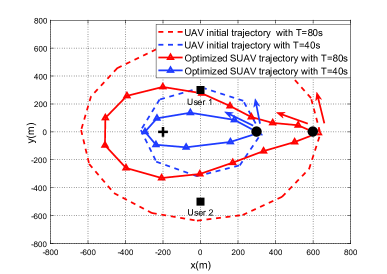
Figure 2: Optimized UAV trajectories for different period $T$ with a single SUAV. Each optimized trajectory is sampled every $5s$ and the sampled points are marked with $\bigtriangleup$. The direction of arrow is the direction of the initial trajectory. The legitimate users locations are marked by $\blacksquare$ and the eavesdropper location is marked by +. In addition, the initial location of UAV is marked by $\mathbin{\vbox{\hbox{\scalebox{1.5}{$\bullet$}}}}$.

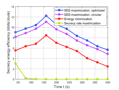
Figure 3: The SEE comparison of different schemes in scenario A.

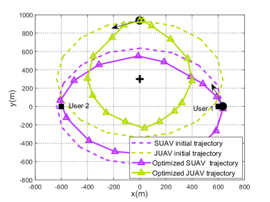
Figure 4: Optimized SUAV trajectory and JUAV trajectory for period $T=80s$. Each optimized trajectory is sampled every $5s$ and the sampled points are marked with $\bigtriangleup$. The direction of arrow is the direction of the initial trajectory. The legitimate users locations are marked by $\blacksquare$ and the eavesdropper location is marked by +. In addition, the initial location of UAV is marked by $\mathbin{\vbox{\hbox{\scalebox{1.5}{$\bullet$}}}}$.

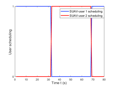
Figure 5: UAV-user scheduling for period $T=80s$.

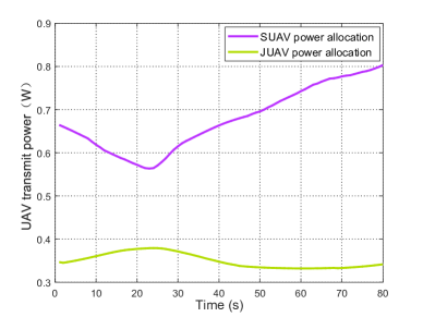
Figure 6: UAV transmit power for period $T=80s$.

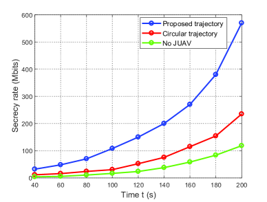
Figure 7: Secrecy rate performance versus different period $T$.

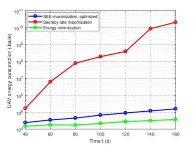
Figure 8: UAV energy consumption versus period $T$ for the One SUAV and One JUAV Case with different schemes.

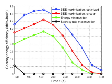
Figure 9: The SEE comparison of different schemes in scenario B.

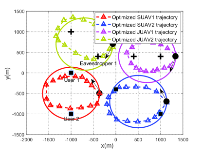
Figure 10: Optimized two SUAV trajectories and two JUAV trajectories for period $T=80s$. Each optimized trajectory is sampled every $5s$ and the sampled points are marked with $\bigtriangleup$. The solid circles are the UAV initial trajectories with same color corresponding its optimized UAV trajectories. The direction of arrow is the direction of the initial trajectory. The legitimate users locations are marked by $\blacksquare$ and the eavesdropper location is marked by +. In addition, the initial location of UAV is marked by $\mathbin{\vbox{\hbox{\scalebox{1.5}{$\bullet$}}}}$.

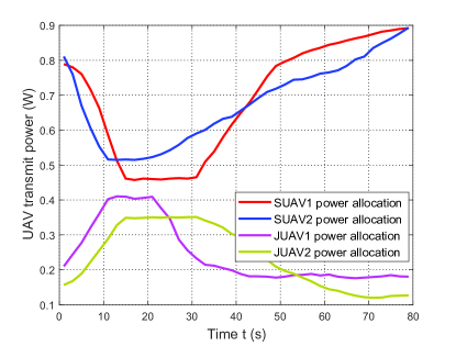
Figure 11: UAV transmit power with SUAV and JUAV for period $T=80s$.

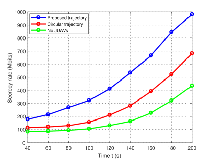
Figure 12: Secrecy rate performance of two SUAVs and two JUAVs versus different period $T$.

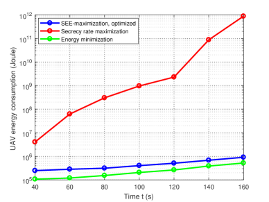
Figure 13: UAV energy consumption versus period $T$ for the Multi-SUAV and Multi-JUAV Case with different schemes.

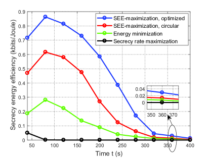
Figure 14: The SEE comparison of different schemes in in scenario C.

IV simulation results

In this section, numerical simulations are provided to evaluate the performance of our proposed scheme. Unless otherwise specified, the corresponding parameter values are summarized in Table I. As will be described later, we consider several network scenarios to study our proposed schemes.

IV-A Single SUAV Case

We first consider one UAV case, where a single SUAV serves multiple legitimate users in the presence of one eavesdropper without the help of JUAV. Fig. 2 shows the optimized UAV trajectories projected onto the horizontal plane for the different period $T$. As expected, the UAV prefers moving closer to the legitimate users and far away from the eavesdropper to improve the system’s secrecy rate. Meanwhile, we can also see that the UAV trajectories are smooth since it is in general less power-consuming[33].

To show the superiority of our proposed scheme in terms of SEE of UAV systems, we consider the following benchmark schemes:

• Optimized SEE maximization scheme: This is our proposed scheme obtained from Algorithm 3 by jointly optimizing the UAV transmit power, user scheduling and UAV trajectory.

• SEE maximization with circular path scheme: For this scheme, the UAV flies with a circular path (initial trajectory). The SEE of UAV systems is obtained by jointly optimizing the UAV transmit power and user scheduling.

• UAV energy consumption minimization scheme: For this scheme, we first obtain the optimized UAV trajectory via minimizing the UAV propulsion energy consumption. Then, with the obtained UAV trajectory, the secrecy rate is optimized by jointly optimizing the UAV transmit power and user scheduling.

• Secrecy rate maximization scheme: The UAV energy consumption is not optimized in this scheme. Our aim is to maximize the secrecy rate by jointly optimizing the UAV transmit power, user scheduling and UAV trajectory.

It is observed from Fig. 3 that for our proposed scheme, the SEE first monotonically increases, and then monotonically decreases with period $T$. This is due to the fact that in the first phase, the incremental of UAV energy consumption is no larger than the incremental of secrecy rate as period $T$ is small, thus increases the system SEE. In the second phase, the incremental of UAV energy consumption is dramatically increased compared with the incremental of secrecy rate as period $T$ becomes larger, thus decreases the system SEE. In addition, we can see that our proposed scheme achieves significantly higher SEE as compared with the benchmarks, which demonstrates the superiority of our proposed scheme.

IV-B One SUAV and One JUAV Case

In this subsection, we consider two UAVs case, where one SUAV and one JUAV simultaneously serve two legitimate users in the presence of one eavesdropper. Evidently, the transmit power of SUAV and JUAV should be carefully designed as the secrecy rate performance of UAV systems will be degraded by the interference imposed by JUAV.

We plot the optimized SUAV trajectory and JUAV obtained from Algorithm 3. It is observed from Fig. 4 that both optimized trajectories are rather similar to the circular trajectory, which has the same result in [33]. In addition, the SUAV prefers moving closer to the legitimate user for data transmitting and JUAV prefers moving closer to eavesdropper to impose strong interference on eavesdropper. Fig. 5 shows that as the SUAV is closer to user 1, the SUAV will transmit information data to user 1 rather than user 2. Similarly, as the SUAV moves closer to user 2, the SUAV tends to transmit information data to user 2 rather than user 1. Fig. 6 shows the power transmit of SUAV and JUAV, as expected, when the SUAV moves from the legitimate user to eavesdropper, less power is allocated. Besides, more JUAV power is transmitted when the SUAV flies closer to the eavesdropper. This is because when the eavesdropper-SUAV channel is good, the stronger jamming signal power needs to be transmitted to interfere the eavesdropper and less power of SUAV is transmitted to prevent the data information wiretapped by the eavesdropper.

Fig. 7 depicts the secrecy rate performance with different period $T$. We compare the following two schemes, namely no cooperative JUAV scheme as well as no trajectory optimization scheme (circular trajectory). Clearly, the secrecy rate is monotonically increasing with time $T$. In addition, our proposed scheme achieves a significant higher secrecy rate than the other two benchmarks, which means the UAV trajectory has prominent impacts on the performance of secrecy rate. Also, for the no cooperative JUAV scheme, the system secrecy rate performance is poor, which indicates that JUAV indeed can bring the performance gain.

In the next, we have performed the new simulations to show the UAV energy consumption of our proposed SEE scheme as compared to other benchmarks. In Fig. 8, it is observed that for secrecy rate maximization scheme, the UAV consumes a large amount of propulsion energy compared with SEE scheme and UAV energy consumption minimization scheme. In addition, the gap between SEE scheme and UAV energy consumption minimization scheme is small, which indicates that the proposed SEE scheme strikes an optimal balance between maximizing the secrecy achievable rate and minimizing the UAV’s propulsion energy consumption. In Fig. 9, we compare the SEE achieved by the four schemes. Similar results can be obtained from Fig. 3, the detailed explanations are omitted here.

IV-C Multi-SUAV and Multi-JUAV Case

A more general case of two SUAVs and two JUAVs to serve multiple legitimate users in the presence of two eavesdroppers is considered in this subsection. Fig. 10 depicts the optimized SUAV and JUAV trajectories obtained by using Algorithm 3. It is observed from Fig. 10 that the trajectories between SUAV 1 and JUAV 2 or (SUAV 2 and JUAV 1) tend to keep away to alleviate the co-channel interference. Meanwhile, the co-channel interference may be beneficial for the secure UAV system by appropriately imposing the jamming signal to the eavesdroppers. The corresponding SUAVs and JUAVs transmit power versus period $T$ are plotted in Fig. 11. First, it is observed that when the distance between legitimate user and eavesdropper is not long (e.g., the legitimate user 1 and eavesdropper 1), the SUAV tends to move closer to legitimate user with less SUAV transmit power and meanwhile the JUAV transmits higher power. Second, when the distance between legitimate user and eavesdropper is long (e.g., the legitimate user 2 and eavesdropper 1), the SUAV tends to move closer to the legitimate user with higher transmit power in order to improve the secrecy rate.

In Fig. 12, the secrecy rate achieved by the various schemes versus period $T$ is plotted. It is first found that our optimized trajectory scheme significantly outperforms the circular trajectory scheme as well as no cooperative JUAVs transmission scheme. In Fig. 13, We plot the UAV energy consumption with different schemes under different period time $T$. We can obtain similar insights in Fig. 8, which further demonstrate its correction. Furthermore, the system SEE performance against SEE maximization with circular path scheme, UAV energy consumption minimization scheme and secrecy rate maximization scheme are shown in Fig. 14. It can be still observed that our proposed scheme achieves significant gain compared with these three benchmarks in terms of SEE. In addition, we can see that the trend of curves in Fig. 14 is similar with Fig. 9, which indicates there exist a fundamental tradeoff between secrecy rate and UAV power consumption.

V Conclusion

This paper investigates the energy-efficient multi-UAV enabled secure transmission wireless systems by considering the UAVs’ propulsion energy consumption and users’ secure rate simultaneously. We aim at maximizing the SEE of UAV systems by jointly optimizing the user scheduling, transmit power and UAV trajectory. Then, an efficient three-layer iterative algorithm is proposed to solve the formulated non-convex and integer fractional problem based on block coordinate descent and Dinkelbach method, as well as SCA techniques. Numerical results show that the UAV mobility is beneficial for achieving higher secure rate than the other benchmarks without considering trajectory optimization. Moreover, three useful insights are extracted from numerical results. First, our proposed JUAVs-aided secrecy rate maximization scheme achieves significantly higher secrecy rate compared with no JUAVs-aided secure scheme. Second, the UAV-enabled SEE does not monotonically increase or decrease with period time $T$, in contrast, the UAV-enabled SEE is firstly increasing with period $T$ and then decreasing with period time $T$. This is different with the secrecy rate maximization scheme and common throughput maximization as in [13]. Third, our proposed SEE scheme gains significantly higher energy efficiency than that of the energy-minimization and secrecy rate maximization schemes.

There are still many other research directions can further extend this work. 1) We model the A2G channel as free path loss for simplicity, the more practical channels such as Rician and Nakagami-m fading can be considered in the future work. 2) The design of UAV altitude can be further exploited, and how to efficiently optimize the joint UAV altitude, transmit power, user scheduling and UAV trajectory is also worthy of investigation. 3) This paper considers the fixed wing UAV, the other types of UAVs such as the rotary wing UAV has the different energy consumption as well as UAV trajectory model, and it is still worthy of investigation. 4) Some literatures have paid attention to investigating the imperfect location of the eavesdropper scenario [48, 49, 50], and how to extend it in our scenario is an interesting work.

Appendix A Proof of Lemma 1

For the sake simplicity, we first define a function $f\left({{x_{1}},\ldots,{x_{N}}}\right)={\log_{2}}\left({\sum\limits_{i=1}^{N}{{a_{i}}{x_{i}}+b}}\right)$, where ${x_{i}}$, ${a_{i}}$, and $b$ are all positive, $\forall i$. It is not difficult to verify that $f\left({{x_{1}},\ldots,{x_{N}}}\right)$ is concave w.r.t. $x_{i},\forall i$, by checking its corresponding Hessian matrix. Recall that the first-order Taylor expansion of a concave function is its global over-estimator [51], i.e., $f\left({{x_{1}},\ldots,{x_{N}}}\right)\leq f\left({x_{1}^{0},\ldots,x_{N}^{0}}\right)+\sum\limits_{i=1}^{N}{{{f^{\prime}}_{{x_{i}}}}\left({x_{1}^{0},\ldots,x_{N}^{0}}\right)\left({{x_{i}}-x_{i}^{0}}\right)}$, where $x_{i}^{0}$, $\forall i$, denotes the feasible point. Thus, we have the following inequality

$${\log_{2}}\left({\sum\limits_{i=1}^{N}{{a_{i}}{x_{i}}+b}}\right) \leq{\log_{2}}\left({\sum\limits_{i=1}^{N}{{a_{i}}x_{i}^{0}+b}}\right)$$

$$+\sum\limits_{i=1}^{N}{\frac{{{a_{i}}{\rm log}_{2}e}}{{\sum\limits_{j=1}^{N}{{a_{j}}x_{j}^{0}+b}}}}\left({{x_{i}}-x_{i}^{0}}\right).$$ (55)

Therefore, (22) follows from (55) by setting $N={{{\cal M}_{2}}\backslash\left\{{{m_{2}}}\right\}\cup{\cal M}_{1}}$, $a_{i}=h_{k_{2},i}[n]$, $x_{i}=p_{i}[n]$, $x_{i}^{0}=p_{i}^{r}[n]$ and $b=\delta^{2}$. This completes the proof of Lemma 1.

References

• [1] A. Filippone, Flight performance of fixed and rotary wing aircraft.   Elsevier, 2006.
• [2] S. Hayat, E. Yanmaz, and R. Muzaffar, “Survey on unmanned aerial vehicle networks for civil applications: A communications viewpoint.” IEEE Communications Surveys and Tutorials, vol. 18, no. 4, pp. 2624–2661, 2016.
• [3] J. Lyu, Y. Zeng, R. Zhang, and J. L. Teng, “Placement optimization of UAV-mounted mobile base stations,” IEEE Communications Letters, vol. 21, no. 3, pp. 604–607, 2017.
• [4] J. Lyu, Y. Zeng, and R. Zhang, “Uav-aided offloading for cellular hotspot,” IEEE Transactions on Wireless Communications, vol. 17, no. 6, pp. 3988–4001, 2018.
• [5] Y. Zeng, X. Xu, and R. Zhang, “Trajectory design for completion time minimization in UAV-enabled multicasting,” IEEE Trans. Wireless Commun, vol. 17, no. 4, pp. 2233–2246, 2018.
• [6] Y. Zeng, R. Zhang, and T. J. Lim, “Throughput maximization for UAV-enabled mobile relaying systems,” IEEE Transactions on Communications, vol. 64, no. 12, pp. 4983–4996, 2016.
• [7] M. Hua, Y. Wang, Z. Zhang, C. Li, Y. Huang, and L. Yang, “Outage probability minimization for low-altitude UAV-enabled full-duplex mobile relaying systems,” China Communications, vol. 15, no. 5, pp. 9–24, 2018.
• [8] M. Alzenad, A. El-Keyi, F. Lagum, and H. Yanikomeroglu, “3-D placement of an unmanned aerial vehicle base station (UAV-BS) for energy-efficient maximal coverage,” IEEE Wireless Communications Letters, vol. 6, no. 4, pp. 434–437, 2017.
• [9] M. Mozaffari, W. Saad, M. Bennis, and M. Debbah, “Efficient deployment of multiple unmanned aerial vehicles for optimal wireless coverage,” IEEE Communications Letters, vol. 20, no. 8, pp. 1647–1650, 2016.
• [10] R. I. Bor-Yaliniz, A. El-Keyi, and H. Yanikomeroglu, “Efficient 3-D placement of an aerial base station in next generation cellular networks,” in IEEE International Conference on Communications (ICC), 2016, pp. 1–5.
• [11] M. Hua, Y. Wang, M. Lin, C. Li, Y. Huang, and L. Yang, “Joint CoMP transmission for UAV-aided cognitive satellite terrestrial networks,” IEEE Access, vol. 7, pp. 14 959–14 968, 2019.
• [12] Q. Wu and R. Zhang, “Common throughput maximization in UAV-enabled OFDMA systems with delay consideration,” IEEE Transactions on Communications, vol. 66, no. 12, pp. 6614–6627, 2018.
• [13] Q. Wu, Y. Zeng, and R. Zhang, “Joint trajectory and communication design for multi-UAV enabled wireless networks,” IEEE Transactions on Wireless Communications, vol. 17, no. 3, pp. 2109–2121, 2018.
• [14] C. Zhan, Y. Zeng, and R. Zhang, “Energy-efficient data collection in UAV enabled wireless sensor network,” IEEE Wireless Communications Letters, vol. 7, no. 3, pp. 328–331, 2018.
• [15] Y. Zeng, J. Xu, and R. Zhang, “Energy minimization for wireless communication with rotary-wing UAV,” IEEE Transactions on Wireless Communications, vol. 18, no. 4, pp. 2329–2345, 2019.
• [16] G. Zhang, Q. Wu, M. Cui, and R. Zhang, “Securing UAV communications via joint trajectory and power control,” IEEE Transactions on Wireless Communications, vol. 18, no. 2, pp. 1376–1389, 2019.
• [17] M. Cui, G. Zhang, Q. Wu, and D. W. K. Ng, “Robust trajectory and transmit power design for secure UAV communications,” IEEE Transactions on Vehicular Technology, vol. 67, no. 9, pp. 9042–9046, 2018.
• [18] D. Yang, Q. Wu, Y. Zeng, and R. Zhang, “Energy tradeoff in ground-to-UAV communication via trajectory design,” IEEE Transactions on Vehicular Technology, vol. 67, no. 7, pp. 6721–6726, 2018.
• [19] Z. Zhu, Z. Chu, N. Wang, S. Huang, Z. Wang, and I. Lee, “Beamforming and power splitting designs for AN-aided secure multi-user MIMO SWIPT systems,” IEEE Transactions on Information Forensics and Security, vol. 12, no. 12, pp. 2861–2874, 2017.
• [20] Z. Zhu, Z. Chu, Z. Wang, and I. Lee, “Outage constrained robust beamforming for secure broadcasting systems with energy harvesting,” IEEE Transactions on Wireless Communications, vol. 15, no. 11, pp. 7610–7620, 2016.
• [21] Z. Zhu, Z. Chu, F. Zhou, H. Niu, Z. Wang, and I. Lee, “Secure beamforming designs for secrecy MIMO SWIPT systems,” IEEE Wireless Communications Letters, vol. 7, no. 3, pp. 424–427, 2018.
• [22] H. Zhang, C. Li, Y. Huang, and L. Yang, “Secure beamforming for SWIPT in multiuser MISO broadcast channel with confidential messages,” IEEE Communications Letters, vol. 19, no. 8, pp. 1347–1350, 2015.
• [23] H. Zhang, Y. Huang, C. Li, and L. Yang, “Secure beamforming design for SWIPT in MISO broadcast channel with confidential messages and external eavesdroppers,” IEEE Transactions on Wireless Communications, vol. 15, no. 11, pp. 7807–7819, 2016.
• [24] K. Cumanan, G. C. Alexandropoulos, Z. Ding, and G. K. Karagiannidis, “Secure communications with cooperative jamming: Optimal power allocation and secrecy outage analysis,” IEEE Transactions on Vehicular Technology, vol. 66, no. 8, pp. 7495–7505, 2017.
• [25] M. Zhang, K. Cumanan, and A. Burr, “Secure energy efficiency optimization for MISO cognitive radio network with energy harvesting,” in IEEE International Conference on Wireless Communications and Signal Processing (WCSP), 2017, pp. 1–6.
• [26] G. Zhang, Q. Wu, M. Cui, and R. Zhang, “Securing UAV communications via trajectory optimization,” in IEEE Global Communications Conference(GLOBECOM), 2017, pp. 1–6.
• [27] Q. Wang, Z. Chen, H. Li, and S. Li, “Joint power and trajectory design for physical-layer secrecy in the UAV-aided mobile relaying system,” IEEE Access, 2018.
• [28] A. Li, Q. Wu, and R. Zhang, “Uav-enabled cooperative jamming for improving secrecy of ground wiretap channel,” IEEE Wireless Communications Letters, to appear, 2018.
• [29] Y. Cai, F. Cui, Q. Shi, M. Zhao, and G. Y. Li, “Dual-UAV enabled secure communications: Joint trajectory design and user scheduling,” IEEE Journal on Selected Areas in Communications, to appear, 2018.
• [30] H. Lee, S. Eom, J. Park, and I. Lee, “Uav-aided secure communications with cooperative jamming,” IEEE Transactions on Vehicular Technology, vol. 67, no. 10, pp. 9385–9392, 2018.
• [31] C. Zhong, J. Yao, and J. Xu, “Secure UAV communication with cooperative jamming and trajectory control,” IEEE Communications Letters, vol. 23, no. 2, pp. 286–289, 2019.
• [32] M. Hua, Y. Wang, Z. Zhang, C. Li, Y. Huang, and L. Yang, “Power-efficient communication in UAV-aided wireless sensor networks,” IEEE Communications Letters, vol. 22, no. 6, pp. 1264–1267, 2018.
• [33] Y. Zeng and R. Zhang, “Energy-efficient UAV communication with trajectory optimization,” IEEE Transactions on Wireless Communications, vol. 16, no. 6, pp. 3747–3760, 2017.
• [34] Z. Sheng, H. D. Tuan, A. A. Nasir, T. Q. Duong, and H. V. Poor, “Power allocation for energy efficiency and secrecy of wireless interference networks,” IEEE Transactions on Wireless Communications, vol. 17, no. 6, pp. 3737–3751, 2018.
• [35] D. Wang, B. Bai, W. Chen, and Z. Han, “Energy efficient secure communication over decode-and-forward relay channels,” IEEE Transactions on Communications, vol. 63, no. 3, pp. 892–905, 2015.
• [36] X. Xu, W. Yang, Y. Cai, and S. Jin, “On the secure spectral-energy efficiency tradeoff in random cognitive radio networks,” IEEE Journal on Selected Areas in Communications, vol. 34, no. 10, pp. 2706–2722, 2016.
• [37] N. T. Nghia, H. D. Tuan, T. Q. Duong, and H. V. Poor, “Mimo beamforming for secure and energy-efficient wireless communication,” IEEE Signal Processing Letters, vol. 24, no. 2, pp. 236–239, 2017.
• [38] L. Xiao, Y. Xu, D. Yang, and Y. Zeng, “Secrecy energy efficiency maximization for UAV-enabled mobile relaying,” arXiv preprint arXiv:1807.04395, 2018.
• [39] L. Qualcomm, “Unmanned aircraft systems-trial report,” 2017.
• [40] 3GPP, “Enhanced LTE support for aerial vehicles,” accessed on Jul. 16, 2017, [Online] Available: ftp://www.3gpp.org/specs/archive/36_series/36.777.
• [41] D. W. Matolak and R. Sun, “Air–ground channel characterization for unmanned aircraft systems part III: The suburban and near-urban environments,” IEEE Transactions on Vehicular Technology, vol. 66, no. 8, pp. 6607–6618, 2017.
• [42] M. C. Grant and S. P. Boyd, “The CVX users guide, release 2.1,” URL http://cvxr. com/cvx/doc/CVX. pdf, 2014.
• [43] W. Dinkelbach, “On nonlinear fractional programming,” Management science, vol. 13, no. 7, pp. 492–498, 1967.
• [44] A. Zappone, E. Björnson, L. Sanguinetti, and E. Jorswieck, “Globally optimal energy-efficient power control and receiver design in wireless networks,” IEEE Transactions on Signal Processing, vol. 65, no. 11, pp. 2844–2859, 2017.
• [45] D. W. K. Ng, E. S. Lo, and R. Schober, “Energy-efficient resource allocation for secure OFDMA systems,” IEEE Transactions on Vehicular Technology, vol. 61, no. 6, pp. 2572–2585, 2012.
• [46] Z.-Q. Luo and P. Tseng, “On the convergence of the coordinate descent method for convex differentiable minimization,” Journal of Optimization Theory and Applications, vol. 72, no. 1, pp. 7–35, 1992.
• [47] J. Gondzio and T. Terlaky, “A computational view of interior point methods,” JE Beasley. Advances in linear and integer programming. Oxford Lecture Series in Mathematics and its Applications, vol. 4, pp. 103–144, 1996.
• [48] H. Kang, J. Joung, J. Ahn, and J. Kang, “Secrecy-aware altitude optimization for quasi-static UAV base station without eavesdropper location information,” IEEE Communications Letters, vol. 23, no. 5, pp. 851–854, 2019.
• [49] Y. Zhou, P. L. Yeoh, H. Chen, Y. Li, R. Schober, L. Zhuo, and B. Vucetic, “Improving physical layer security via a UAV friendly jammer for unknown eavesdropper location,” IEEE Transactions on Vehicular Technology, vol. 67, no. 11, pp. 11 280–11 284, 2018.
• [50] T.-X. Zheng, H.-M. Wang, and Q. Yin, “On transmission secrecy outage of a multi-antenna system with randomly located eavesdroppers,” IEEE Communications Letters, vol. 18, no. 8, pp. 1299–1302, 2014.
• [51] S. Boyd and L. Vandenberghe, Convex optimization.   Cambridge university press, 2004.