Throughput Maximization for UAV-aided Backscatter Communication Networks

Abstract

This paper investigates unmanned aerial vehicle (UAV)-aided backscatter communication (BackCom) networks, where the UAV is leveraged to help the backscatter device (BD) forward signals to the receiver. Based on the presence or absence of a direct link between BD and receiver, two protocols, namely transmit-backscatter (TB) protocol and transmit-backscatter-relay (TBR) protocol, are proposed to utilize the UAV to assist the BD. In particular, we formulate the system throughput maximization problems for the two protocols by jointly optimizing the time allocation, reflection coefficient and UAV trajectory. Different static/dynamic circuit power consumption models for the two protocols are analyzed. The resulting optimization problems are shown to be non-convex, which are challenging to solve. We first consider the dynamic circuit power consumption model, and decompose the original problems into three sub-problems, namely time allocation optimization with fixed UAV trajectory and reflection coefficient, reflection coefficient optimization with fixed UAV trajectory and time allocation, and UAV trajectory optimization with fixed reflection coefficient and time allocation. Then, an efficient iterative algorithm is proposed for both protocols by leveraging the block coordinate descent method and successive convex approximation (SCA) techniques. In addition, for the static circuit power consumption model, we obtain the optimal time allocation with a given reflection coefficient and UAV trajectory and the optimal reflection coefficient with low computational complexity by using the Lagrangian dual method. Simulation results show that the proposed protocols are able to achieve significant throughput gains over the compared benchmarks.

I Introduction

In wireless powered communication networks (WPCNs), energy-constrained sensors powered by radio frequency (RF) signals have been widely investigated due to their ability to provide reliable energy to Internet of Thing (IoT) devices[2, 3, 4, 5, 6, 7, 8]. In WPCNs, the sensor nodes harvest the transmitted signal energy, and then transmit the data to a receiver by generating radio waves with the help of active RF components. However, active RF components integrated into the sensor nodes can still consume significant energy for data forwarding. More energy-efficient devices, called backscatter devices (BDs), have received significant attention in the past decade as a promising technique for IoT [9, 10, 11, 12]. Compared with traditional wireless powered devices that transmit signals to the receiver by generating radio waves with the help of active RF components, the circuit power consumption of a BD integrated with passive components is several orders of magnitude lower, and can significantly prolong IoT lifetimes [13], [14]. A typical application of backscatter communication (BackCom) for IoT is in RF identification (RFID) scenarios. More specifically, the RF reader first transmits the RF signals to a passive tag, the tag harvests energy from the RF reader signal to power its circuit, and then forwards the information bits carried on the received RF sinusoidal signal back to the reader by adjusting its load impedance to change the amplitude and phase of its backscattered signal[15], [16].

In [13], a BackCom system design was presented that leverages ambient RF sources such as TV station, cellular base stations (BS), WiFi access point, etc. Although there are many benefits in backscatter-based communication systems, one must address a number of technical challenges ranging from the circuit design of the tags to designing the required transmission protocols. For example, the authors in [17] studied two RF energy harvesting circuit prototypes, and the sensor measurements from the two prototypes were tested from different locations in a real-world scenario. The results showed that the most sensitive RF harvesting sensor node can be operated at $200\rm m$ from a traditional BS. In [11], a cooperative BackCom relaying system was studied, and the system throughput was maximized via optimal time allocation. In [9], the same authors studied a BackCom-aided duty cycle protocol in which the BD either remained in a sleep or active state, and the throughput maximization problem was formulated by jointly optimizing the sleep/active state and reflection coefficient. A backscatter-aided cognitive wireless powered network was investigated in [18], where a hybrid harvest-then-transmit protocol was proposed, and the optimal time allocation for energy harvesting and backscatter communication was derived. In [19], the authors studied a relay-assisted secure BackCom network for maximizing the secrecy rate of the system, and a sub-optimal low-complexity relay selection strategy was obtained based on the distance between the forward and reverse links. There has been considerable work on BackCom systems like that described above which assumes the existence of available RF power sources such as TV or BS transmission towers. However, in remote or underdeveloped areas, no such power sources may be available for providing RF energy to IoT BDs.

In this paper, we address some of the challenges necessary for communication among IoT devices. A promising solution involves leveraging the unmanned aerial vehicles (UAVs) to act as RF power resources to assist communication between the BD and receiver. UAVs have already received significant attention both from academia and industry for various applications such as energy transmission, data collection, hot spot offloading and wireless communications [20, 21, 22, 23, 24, 25, 26, 27, 28, 29, 30, 31, 32, 33]. The UAV’s flexible mobility can be exploited to design a trajectory that increases network throughput. For example, the work in [24] proposed to use a UAV as a mobile BS to serve cell-edge users and offload data from traditional BS. Their numerical results showed that the common throughput was significantly improved by optimizing the UAV trajectory, bandwidth allocation and user partitioning. A similar problem was addressed in [25], where the UAV acted as a relay to assist data transmission, and its trajectory and the source/relay power allocation were optimized. The results showed that the UAV trajectory provided significant gains in terms of system throughput. A UAV integrated into satellite-based cognitive terrestrial network was considered in [26], assuming the UAV and BS cooperatively serve a terrestrial user by sharing the licensed satellite network spectrum. This work showed that by carefully designing the UAV trajectory and BS/UAV power allocation, the throughput of secondary networks can be significantly improved. A multi-UAV enabled system for serving multiple users was also shown in [27] to improve throughput by carefully designing the UAV trajectories and power allocation.

In this paper, we study a UAV-aided BackCom network, in which the UAV is leveraged to assist data transmission from BD to receiver. Our work is different from [34], which considered a UAV-enabled WPCN where the UAV is used to first charge the sensors in the downlink and then receive data in the uplink. In our work, we exploit a UAV to improve the communication connectivity between the BD and receiver in scenarios both with and without a direct connection between the two. For the first case, the direct link between BD and receiver is assumed to be available and modeled as a channel consisting of both distance-dependent path-loss and small-scale Rayleigh fading. We propose a transmit-backscatter (TB) protocol for this case where the UAV first transmits signals to the BD, and the BD directly reflects the signals to the receiver by adjusting the load impedance of BD to change the amplitude and phase of the backscattered signal. For the second case, the direct link between BD and receiver is unavailable caused by severe blockage. We propose a transmit-backscatter-relay (TBR) protocol for this case, in which the UAV transmits signals to the BD, the BD returns the signals back to the UAV, and the UAV then decodes the signals and forwards the signals to the receiver. Therefore, the resulting problems for maximizing the capacity of BackCom networks for these two cases are distinctly different, which are discussed separately later in this paper. Nevertheless, the joint design of UAV trajectory, BD’s backscattering time and reflecting coefficient can significantly improve the BackCom networks capacity for both two cases. On the one hand, the UAV can adjust its location to establish the stronger UAV-BD link. As a result, more energy can be harvested at BD for backscattering its own data to the receiver. On the other hand, due to the practical constraints such as final/initial UAV location and flying period, the UAV is not capable of hovering above the BD all the time. Therefore, the BD’s backscattering time and reflecting coefficient should be adaptively designed according to the movement of the UAV trajectory. For example, when the UAV is far way from the BD, the BD’s backscattering time and reflecting power should be reduced, whereas when the UAV hovers above the BD, the BD’s backscattering time and reflecting power will be increased. It is worth pointing out that there generally exists a trade-off for the reflection coefficient between energy harvesting and backscattering rate [9]. Note that a stronger reflection coefficient means that the backscattering rate increases but less energy is harvested, and reducing the harvested energy also reduces the time required for data forwarding.

Motivated by above, our goal is to maximize the BackCom networks capacity for both two cases by jointly optimizing the UAV trajectory, time allocation and reflection coefficient over a finite flight period of the UAV, subject to the UAV mobility and practical harvest-backscatter constraints. Due to the BD’s backscattering time is highly related to the BD’s circuit power consumption. Therefore, the precise modeling on the circuit power consumption for the system design is of paramount importance. Specifically, we consider two circuit power consumption models, namely static and dynamic models, in this paper. For the static model, the BD’s circuit power consumption is fixed regardless of the transmission rate. For the dynamic model, the BD’s circuit power consumption is a function of the transmission rate [10]. The main contributions are summarized as follows:

• We propose two protocols for the direct link available case and direct link unavailable case in the UAV-aided BackCom networks. Compared to the existing BackCom, this paper is first to exploit the UAV to improve the BackCom networks capacity via joint optimization of UAV trajectory, time allocation and reflection coefficient.

• We develop a three-layer iterative algorithm to solve the resulting non-convex optimization problems for both models by using the block coordinate descent method and successive convex approximation (SCA) techniques. Specifically, we decompose the formulated problem into three sub-problems: time allocation optimization with fixed UAV trajectory and reflection coefficient, reflection coefficient optimization with fixed UAV trajectory and time allocation, and UAV trajectory optimization with fixed reflection coefficient and time allocation. Based on the solutions to the three sub-problems, a block coordinate descent method is proposed for alternately optimizing time allocation, reflection coefficient and UAV trajectory to maximize the total system throughput.

• We consider both static and dynamic power consumption models for the BD. For the static circuit power consumption model, where the value of circuit power consumption is constant, we derive the optimal time allocation in closed form, and the optimal reflection coefficient using a low-complexity Lagrangian dual method for both protocols.

This paper is organized as follows. Section II introduces the system model and problem formulation. Section III considers the first case where a direct link between BD and receiver is available. Section IV considers the second case where a direct link is unavailable. Numerical results are presented in Section V, and the conclusions are given in Section VI.

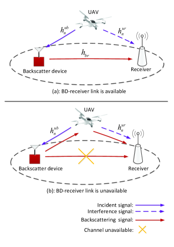
Figure 1: UAV-aided transmission in BackCom networks

II System Model AND PROBLEM FORMULATION

II-A System Model

We consider a UAV-aided BackCom network that consists of one BD, one receiver and one UAV as shown in Fig. 1. We assume that the UAV can freely adjust its heading to move with a fixed altitude $H$. We assume that a finite flight period of the UAV is $T$. To make the problem tractable, the period $T$ is equally divided into $N$-length time slots of duration $\delta=T/N$. As a consequence, the horizontal location of UAV at time slot $n$ is denoted as ${\bf q}_{n}$, $n\in{\cal N}=\{1,...,N\}$. The horizontal coordinates of the BD and receiver are fixed at ${\bf w}_{b}$ and ${\bf w}_{r}$, respectively.

The UAV is likely to establish line-of-sight (LoS) links for both air-to-ground (A2G) and ground-to-air (G2A) channels as reported in [35],[36]. Therefore, we model the A2G and G2A channels as Rician fading [21],[37]. Let $\sqrt{h_{n}^{ub}}$ and $\sqrt{h_{n}^{ur}}$ denote the UAV-BD and UAV-receiver channel coefficients at time slot $n$, respectively. The Rician fading consists of both distance-dependent path-loss and small-scale fading, which can be expressed as

$$\sqrt{h_{n}^{uf}}=\sqrt{{\theta_{n}^{uf}}}{\tilde{h}}_{n}^{uf},$$ (1)

where $f\in\{b,r\}$, and ${\theta_{uf}}\left[n\right]$ accounts for large-scale channel attenuation that depends on the path loss and shadowing at time slot $n$, and ${\tilde{h}}_{n}^{uf}$ is a complex-valued random variable with ${\mathbb{E}}\left[{{{\|{\tilde{h}_{n}^{uf}}\|}^{2}}}\right]=1$ that represents small-scale channel attenuation at time slot $n$. Specifically, ${{\theta_{n}^{uf}}}$ can be written as

$${\theta_{n}^{uf}}=\frac{{{\beta_{0}}}}{{{{\left\|{{{\bf{q}}_{n}}-{{\bf{w}}_{f}}}\right\|}^{2}}+{H^{2}}}},$$ (2)

where $\beta_{0}$ represents the reference channel gain at $d=1$ meter (m). Despite the result in [38] shown that the path loss exponents of A2G and G2A are different, the gap between A2G and G2A for path loss exponent is very small. We thus assume that the two path loss exponents are same with 2 that is consistent with the most literatures adopted [20, 21, 24, 25, 26, 27, 31, 33, 37]. Although we assume that the path-loss exponent is 2, it can be easily extended to other cases based on the results in Section II-A of [39]. Obviously, the value ${\theta_{n}^{uf}}$ depends on the distance between UAV and BD/receiver. The small-scale fading can be modeled as below

$$\tilde{h}_{n}^{uf}=\sqrt{\frac{{{K_{n}}}}{{{K_{n}}+1}}}{{\tilde{h}}}+\sqrt{\frac{1}{{{K_{n}}+1}}}\tilde{\tilde{h}},$$ (3)

where ${{\tilde{h}}}$ denotes the deterministic LoS channel coefficient with $\|{{{\tilde{h}}}}\|=1$, and $\tilde{\tilde{h}}$ is a circularly symmetric complex Gaussian random variable with mean zero and variance 1, and $K_{n}$ is a Rician factor at time slot $n$. For a sufficiently large value $K_{n}$, the channel model approximately equals to free-space path loss model. For $K_{n}=0$, the Rician channel model is simplified as Rayleigh channel model. The Rician factor can be assumed to be invariant, namely $K=K_{n}$ for all $n$, for the following reasons. First, for the rural areas and the limited serving range from several meters to dozens of meters in BackCom system, the Rician factor can be approximately treated to be independent of the varying UAV locations. Second, for the long period time $T$, the most time for UAV is to stay stationary above the BD, thus by assuming $K=K_{n}$ for all $n$ is reasonable.

We further assume that the channel model between BD and receiver follows Rayleigh fading with channel power gain denoted by ${h_{br}}={\beta_{0}}d_{br}^{-m}\xi$, where $d_{br}$ is the distance between BD and receiver, $m$ denotes the path loss exponent, and $\xi$ is an exponentially distributed random variable with mean 1.

In the following, we introduce the main constraints that need to be considered for the Backcom networks.

Energy harvesting and circuit power consumption constraint: Assuming that the UAV transmit power is $P$, the average received RF power by BD at time slot $n$ can be calculated as $P\mathbb{E}\left[{h_{n}^{ub}}\right]$. One part of the harvested energy is used to power the BD’s circuit power consumption, and the remaining harvested energy is used to backscatter its own data [9], [10]. The harvested energy used for powering the BD’s circuit is given by

$${E_{n}^{b}}\left[n\right]=\eta\left({1-{a_{n}}}\right)P\mathbb{E}\left[{h_{n}^{ub}}\right]=\eta\left({1-{a_{n}}}\right)P\theta_{n}^{ub},$$ (4)

where $a_{n}$ denotes the reflection coefficient at time slot $n$ ($0\leq a_{n}\leq 1$), and $\eta$ represents the energy harvesting efficiency. Specially, $a_{n}=0$ indicates that all the harvested energy is used to power the BD’s circuit power consumption and no power is left to backscatter signals. $a_{n}=1$ indicates all the harvested energy is used to backscatter signals and no power is left to power the BD’s circuit power consumption. Note that the reflection coefficient $a_{n}$ is controllable by changing the impedance of an antenna in the presence of an incident signal [9],[10].

In order for BD to work, assuming that the signal processing delay at the BD is one time slot, we have the following constraint

$$\sum\limits_{i=1}^{n}{{\varphi_{i{\rm{+}}1}}P_{i{\rm{+}}1}^{e}}\leq\sum\limits_{i=1}^{n}{E_{i}^{b}\left[n\right]},n{\rm{=}}1,\ldots,N-1,$$ (5)

where $\varphi_{i+1}$ denotes the portion of the BD’s backscattering period for time slot $i+1$, and $P^{e}_{i+1}$ denotes the BD circuit power consumption at time slot $i+1$. The left hand side of (5) stands for the BD’s circuit power consumption, and the right hand side of (5) stands for the BD’s harvested energy. The constraint (5) shows that at each time slot $n$, the BD can be powered to work by using the harvested energy in the previous time slot. Note that as shown in [10], the BD’s dynamic circuit energy consumption is given by

$$P_{i{\rm{+}}1}^{e}={P_{\varepsilon}}+\mu{R_{i+1}},$$ (6)

where $P_{\varepsilon}$ denotes the static energy consumption, $\mu$ is a non-negative weight factor [10], and $R_{i+1}$ is the backscattering rate at time slot $i+1$. For $\mu=0$, namely static circuit energy consumption model, the BD’s circuit energy consumption is fixed with $P_{\varepsilon}$. As a result, substituting (4) and (6) into (5), we have

$$\sum\limits_{i=1}^{n}{{\varphi_{i+1}}\left({{P_{\varepsilon}}+\mu{R_{i+1}}}\right)}\leq\sum\limits_{i=1}^{n}{\eta\left({1-{a_{i}}}\right)}P\theta_{i}^{ub}.$$ (7)

UAV mobility constraint: The UAV mobility is constrained by its maximum flying speed, which implies that

$$\left\|{{\bf{q}}_{n+1}-{\bf{q}}_{n}}\right\|\leq{V_{\max}}\delta,~{}n=0,\ldots,N-1,$$

$${\bf{q}}_{0}={{\bf{q}}_{\rm I}},{\bf{q}}_{N}={{\bf{q}}_{\rm{F}}},$$ (8)

where $V_{\rm max}$ denotes the maximum UAV speed, ${{\bf{q}}_{\rm I}}$ and ${{\bf{q}}_{\rm{F}}}$ represent the UAV’s initial and final location, respectively.

Next, we will separately discuss models of the two cases, namely direct link available and unavailable case.

II-A1 Direct Link Available Between BD and Receiver

In this case, the UAV acts as a mobile energy transmitter to charge the BD and assist the BD for data backscatter transmission as shown in Fig. 1 (a). Different from the traditional devices that can generate the new RF radios, the BD can only leverage the ambient RF signal to backscatter its own data [13]. Therefore, the BD cannot operate in the frequency division duplexing (FDD) model due to the fact that the BD uses the same frequency band for both the uplink and downlink. Here, we use time-division duplexing (TDD) model, and we further assume that other co-channel RF sources are not present. We propose a transmit-backscatter (TB) protocol, which consists of two stages. In the first stage, the BD receives the broadcasting signals from the UAV. In the second stage, the BD backscatters its own data by riding on the previously broadcasting signals to the receiver.

Specifically, in the first stage, at any time slot $n$, the received signal at the BD from the UAV is given by

$$y_{n}^{b}=\sqrt{P}\sqrt{h_{n}^{ub}}{x_{n}},$$ (9)

where $P$ is the UAV’s maximum transmit power, and $x_{n}$ denotes the UAV’s transmitted signal at time slot $n$ with $\|x_{n}\|^{2}=1$. Note that the noise received at the BD is neglected because the BD’s circuit only includes passive components [10],[40], and [41].

In the second stage, at time slot $n+1$, the received signal at the receiver from the BD is given by

$$y_{n+1}^{r}=\sqrt{h_{br}}\sqrt{{a_{n}}}y_{n}^{b}{c_{n}}+\sqrt{P}\sqrt{h_{n}^{ur}}{x_{n}}+{n_{r}},$$ (10)

where $a_{n}$ denotes the BD’s reflection coefficient at time slot $n$, $n_{r}$ represents the received noise at the receiver with power $\sigma_{r}^{2}$, and $c_{n}$ represents the BD’s own data with $\|c_{n}\|^{2}=1$. The term $\sqrt{P}\sqrt{h_{n}^{ur}}{x_{n}}$ denotes the received signal from the UAV at time slot $n$. Note that at the second stage, the UAV does not broadcast any signals since the BD operates at half-duplex mode. Substituting (9) into (10), we have

$$y_{n+1}^{r}{\rm{=}}\sqrt{h_{br}}\sqrt{{a_{n}}}\sqrt{P}\sqrt{h_{n}^{ub}}{x_{n}}{c_{n}}+\sqrt{P}\sqrt{h_{n}^{ur}}{x_{n}}+{n_{r}}.$$ (11)

The strength of the backscattering signal received at receiver from the BD is generally much lower than that received from the UAV. Thus, the successive interference cancellation (SIC) technique can be applied. Specifically, the receiver first decodes the UAV signals and then subtracts it from the combined signals before decoding its own signals [9, 10, 11]. Thus, the signal-plus-noise ratio (SNR) at the receiver at time slot $n+1$ can be expressed as

$$\gamma_{n+1}^{r}=\frac{{P{a_{n}}h_{br}h_{n}^{ub}}}{{\sigma_{r}^{2}}}.$$ (12)

Note that since the channel power gains ${h_{br}}$ and $h_{n}^{ub}$ are the random variables, the instantaneously achievable rate is also a random variable, we thus pay attention to obtaining the expected communication throughput. The expected rate of the receiver at time slot $n+1$ is given by

$$R_{n+1}^{r}={\mathbb{E}}\left[{{{\log}_{2}}\left({1+\gamma_{n+1}^{r}}\right)}\right]{\rm{}}.$$ (13)

The closed-form expressions of $R_{n+1}^{r}$ in (13) and even its lower bound result of $R_{n+1}^{r}$ are unsolvable due to the difficulty of deriving its probability distribution. To address this issue, one feasible approach is to use an approximation result of $R_{n+1}^{r}$. We have the following Theorem:

Theorem 1

The approximation result of $R_{n+1}^{r}$, denoted as $\hat{R}_{n+1}^{r}$, is given by

$$\hat{R}_{n+1}^{r}={\log_{2}}\left({1+\frac{{{W_{br}}{a_{n}}}}{{{{\left\|{{{\bf{q}}_{n}}-{{\bf{w}}_{b}}}\right\|}^{2}}+{H^{2}}}}}\right),$$ (14)

where ${W_{br}}=\frac{{{e^{-{\kappa_{0}}}}P{\beta_{0}}}}{{{\lambda_{br}}\sigma_{r}^{2}}}$.

Proof:

Please refer to Appendix A. ∎

The accuracy for the approximation in Theorem 1 will be evaluated in Section V under different parameters.

II-A2 Direct Link Unavailable Between BD and Receiver

In this case, we consider the scenario where a direct link between BD and receiver is unavailable. The UAV acts as a relay to assist the BD for backscattering data to the receiver using a decode-and-forward (DF) manner as shown in Fig. 1 (b). We propose a transmit-backscatter-relay (TBR) protocol, which consists of three stages. In the first stage, the UAV transmits broadcasting signals to the BD. In the second stage, the BD backscatters the own data via riding on the previously broadcasting signals to the UAV. Note that in this stage, the UAV only receives the signals and does not transmit broadcasting signals since the UAV operates in the half-duplex mode. In the third stage, the UAV acts as a relay to transmit the previously received BD’s data to the receiver. Specifically, in the first stage, at time slot $n$, the UAV transmits signals to the BD, and the received signal at BD is given by

$$z_{n}^{b}=\sqrt{P}\sqrt{h_{n}^{ub}}{x_{n}},$$ (15)

where $P$ is the UAV’s maximum transmit power, $x_{n}$ is the UAV broadcasting signal at time slot $n$ with $\|x_{n}\|^{2}=1$. In the second stage, at time slot $n+1$, the BD forwards its own data by riding on the previously UAV broadcasting signal to the UAV, the received signal at the UAV is given by

$$z_{n+1}^{u}=\sqrt{h_{n+1}^{ub}}\sqrt{{a_{n}}}z_{n}^{b}{c_{n}}+{n_{u}},$$ (16)

where $a_{n}$, $c_{n}$, and $n_{u}$ represent reflection coefficient, BD’s transmit data, and received noise at time slot $n$, respectively. The noise power of $n_{u}$ is $\sigma_{u}^{2}$. Substituting (15) into (16), we have

$$z_{n+1}^{u}{\rm{=}}\sqrt{P{a_{n}}h_{n+1}^{ub}h_{n}^{ub}}{x_{n}}{c_{n}}+{n_{u}}.$$ (17)

Similar as previous discussion on the direct link case, we are interested in the expected rate. The expected rate from BD to UAV at time slot $n+1$ is given by

$$\check{R}_{n+1}^{u}=\mathbb{E}\left[{{{\log}_{2}}\left({1+\frac{{P{a_{n}}h_{n+1}^{ub}h_{n}^{ub}}}{{\sigma_{u}^{2}}}}\right)}\right].$$ (18)

We assume that the UAV is capable of correctly decoding the BD’s signal $c_{n}$ at any time slot $n+1$. In the third stage, at time slot $n+2$, the UAV transmits its decoded BD’s data to the receiver, the received signal at the receiver is given by

$$z_{n+1}^{r}{\rm{=}}\sqrt{{P}}\sqrt{h_{n+2}^{ur}}{s_{n+2}}+{\rm{}}\sqrt{{P}}\sqrt{h_{n}^{ur}}{x_{n}}+{n_{r}},$$ (19)

where $s_{n+2}$ denotes UAV’s transmitted signal at time slot $n$, namely $s_{n+2}=c_{n}$. The term $\sqrt{P}\sqrt{h_{n}^{ur}}{x_{n}}$ denotes the received signal from the UAV at previous time slot $n$. Similarly, the SIC technique is also applied at the receiver, which has been previously discussed in (11). The expected transmission rate from UAV to receiver at time slot $n+2$ is thus given by

$$\check{R}_{n+2}^{r}=\mathbb{E}\left[{{{\log}_{2}}\left({1+\frac{{Ph_{n+2}^{ur}}}{{\sigma_{r}^{2}}}}\right)}\right].$$ (20)

To make the problem more tractable, we write ${\check{R}}^{u}_{n+1}$ in (18) as $\check{R}_{n+1}^{u}=\mathbb{E}\left[{{{\log}_{2}}\left({1+\frac{{P{a_{n}}{{\left({h_{n+1}^{ub}}\right)}^{2}}}}{{\sigma_{u}^{2}}}}\right)}\right]$ by assuming that $h^{ub}_{n+1}\cong h^{ub}_{n}$. Generally, it is challenging to obtain the probability distributions of $\check{R}_{n+1}^{u}$ and $\check{R}_{n+2}^{r}$. Similar as in Theorem 1, the approximation results for $\check{R}_{n+1}^{u}$ and $\check{R}_{n+2}^{r}$, denoted as $R_{n+1}^{u}$ and $R_{n+2}^{r}$, can be respectively given by

$$R_{n+1}^{u}={\log_{2}}\left({1+\frac{{P{a_{n}}{{\left({\theta_{n+1}^{ub}}\right)}^{2}}}}{{\sigma_{u}^{2}}}}\right),$$ (21)

and

$$R_{n+2}^{r}={\log_{2}}\left({1+\frac{{P\theta_{n+2}^{ur}}}{{\sigma_{r}^{2}}}}\right).$$ (22)

The derivations for (21) and (22) are similar to that of Theorem 1, and are omitted here for brevity. Section V shows that the approximation results match well with the numerical results.

II-B Problem Formulation

For the direct link available case, our objective is to maximize the sum of ergodic capacity by jointly optimizing the UAV trajectory, time allocation and reflection coefficient under the energy harvesting and circuit power consumption constraint as well as UAV mobility constraint. Define ${\cal N}_{1}=\{1,2,..,N/2\}$. The problem is formulated as follows.

$$\left({{\rm{P1}}}\right)\mathop{\max}\limits_{a_{2n-1},\varphi_{2n},{\bf q}_{n}}\sum\limits_{n=1}^{N/2}{\varphi_{2n}\hat{R}^{r}_{2n}}$$

$${\rm s.t.}~{}\sum\limits_{i=1}^{n}{{\varphi_{2i}}\left({{P_{\varepsilon}}+\mu\hat{R}_{2i}^{r}}\right)}\leq\sum\limits_{i=1}^{n}{\eta\left({1-{a_{2i-1}}}\right)}P\theta_{2i-1}^{ub},n\in{{\cal N}_{1}},$$ (23)

$$\quad 0\leq a_{2n-1}\leq 1,n\in{\cal N}_{1},$$ (24)

$$\quad 0\leq\varphi_{2n}\leq 1,n\in{\cal N}_{1},$$ (25)

$$\quad\eqref{Case1_constr2},$$

where (23) denotes the energy harvesting and circuit power consumption constraint discussed in Section II.A, (24) and (25) represent the BD’s backscattering coefficient and backscattering time constraints, respectively.

Similarly, for the direct link unavailable case, we aim to maximize the sum of ergodic capacity by jointly optimizing the UAV trajectory, time allocation and reflection coefficient under some specified constraints. Define ${\cal N}_{2}=\{1,2,..,N/3\}$. Mathematically, the optimization problem is formulated as

$$\left({{\rm{P2}}}\right)\mathop{\max}\limits_{{a_{3n-2}},{\varphi_{3n-1}},{\bf{q}}\left[n\right]}\sum\limits_{n=1}^{{N\mathord{\left/{\vphantom{N3}}\right.\kern-1.2pt}3}}{{\varphi_{3n-1}}R_{3n-1}^{u}}$$

$${\rm s.t.}~{}\sum\limits_{i=1}^{n}{{\varphi_{3i-1}}\left({{P_{\varepsilon}}+\mu R_{3i-1}^{r}}\right)}\leq$$

$$\qquad\qquad\qquad\sum\limits_{i=1}^{n}{\eta\left({1-{a_{3i-2}}}\right)}P\theta_{3i-2}^{ub},n\in{{\cal N}_{2}},$$ (26)

$$\qquad\sum\limits_{i=1}^{n}{\varphi_{3i-1}R_{3i-1}^{u}}\leq\sum\limits_{i=1}^{n}{R_{3i}^{r}},n\in{\cal N}_{2},$$ (27)

$$\qquad 0\leq a_{3n-2}\leq 1,n\in{\cal N}_{2},$$ (28)

$$\qquad 0\leq\varphi_{3n-1}\leq 1,n\in{\cal N}_{2},$$ (29)

$$\qquad\eqref{Case1_constr2},$$

where (26) represents the energy harvesting and circuit power consumption constraint discussed in Section II.A, and (27) denotes the information-casuality constraint by assuming that the signal processing delay at the UAV is one time slot. (28) and (29) stand for the backscattering coefficient and backscattering time constraints, respectively.

Problems $(\rm P1)$ and $(\rm P2)$ are highly non-convex optimization problems where the optimization variables are intricately coupled in the objective function and constraints. Specifically, first, the UAV trajectory, BD’s backscattering time, and BD’s reflecting coefficient are closely coupled in the objective function in $(\rm P1)$ or $(\rm P2)$, which results in non-convexity of $(\rm P1)$ or $(\rm P2)$. In addition, the constraints (23) and (26) are also non-convex with respect to (w.r.t.) UAV trajectory, BD’s backscattering time as well as BD’s reflecting coefficient. In generally, there is no standard method for solving such non-convex optimization problems optimally. In Sections III and IV, we propose an alternating optimization algorithms for solving problems $(\rm P1)$ and $(\rm P2)$, respectively.

III Proposed Algorithm For Problem $(\rm P1)$

In this section, we consider problem $(\rm P1)$ for the direct link available case. Problem $(\rm P1)$ is challenging to solve due to the non-convex objective function and constraint (23). To this end, we decompose $(\rm P1)$ into three sub-problems, namely time allocation optimization with fixed UAV trajectory and reflection coefficient, reflection coefficient optimization with fixed UAV trajectory and time allocation, and UAV trajectory optimization with fixed reflection coefficient and time allocation. Based on the solutions to the three sub-problems, a block coordinate descent method is proposed for alternately optimizing the time allocation, reflection coefficient and UAV trajectory to maximize the total system throughput.

III-1 Time allocation optimization

For any given UAV trajectory $\{{\bf q}_{n}\}$ and reflection coefficient $\{a_{2n-1}\}$, the time allocation $\{\varphi_{2n}\}$ of problem $(\rm P1)$ can be optimized by solving the following problem

$$\left({{\rm{P1}}{\rm{.1}}}\right)\mathop{\max}\limits_{\varphi_{2n}}\sum\limits_{n=1}^{N/2}{\varphi_{2n}{{\log}_{2}}\left({1+\frac{{{W_{br}}a_{2n-1}}}{{{{\left\|{{\bf{q}}_{2n-1}-{{\bf{w}}_{b}}}\right\|}^{2}}+{H^{2}}}}}\right)}$$

$$\qquad{\rm s.t.}~{}\eqref{Case1_constr1},\eqref{Case1_constr4}.$$

Since problem $(\rm P1.1)$ is a standard linear programming problem, it can be efficiently solved by interior point method [42].

Theorem 2

For the static circuit energy consumption model, namely $\mu=0$, if $\hat{R}^{r}_{2n}$ is a decreasing function with $n\in{\cal N}_{1}$, the optimal solution $\{\varphi_{2n}^{*}\}$ to problem $(\rm P1.1)$ is given by

$$\varphi_{2n}^{*}=\left[{\frac{{\eta\left({1-{a_{2n-1}}}\right)P\theta_{2n-1}^{ub}}}{{{P_{c}}}}}\right]_{0}^{1},n\in{\cal N}_{1}.$$ (30)

Proof:

Please refer to Appendix B. ∎

Theorem 2 shows that the equality in (23) must hold at any time $n$, which means that the energy harvested by the BD at time slot $n$ from the UAV will be thoroughly depleted for the BD’s data backscattering transmission at time slot $n+1$. This transmission approach is similar to the time switching-based relaying (TSR) protocol of [43].

III-2 Reflection coefficient optimization

For any given UAV trajectory $\{{\bf q}_{n}\}$ and time allocation $\{\varphi_{2n}\}$, the reflection coefficient $\{a_{2n-1}\}$ of problem $(\rm P1)$ can be optimized by solving the following problem

$$\left({{\rm{P1}}.2}\right)\mathop{\max}\limits_{{a_{2n-1}}}\sum\limits_{n=1}^{N/2}{{\varphi_{2n}}{{\log}_{2}}\left({1+\frac{{{W_{br}}{a_{2n-1}}}}{{{{\left\|{{{\bf{q}}_{2n-1}}-{{\bf{w}}_{b}}}\right\|}^{2}}+{H^{2}}}}}\right)}$$

$$\qquad{\rm s.t.}~{}\eqref{Case1_constr1},\eqref{Case1_constr3}.$$

Despite the objective function ${{{\log}_{2}}\left({1+\frac{{{W_{br}}{a_{2n-1}}}}{{{{\left\|{{{\bf{q}}_{2n-1}}-{{\bf{w}}_{b}}}\right\|}^{2}}+{H^{2}}}}}\right)}$ is concave w.r.t. $a_{2n-1}$, the constraint (23) is non-convex w.r.t. $a_{2n-1}$. In general, there is no efficient method to obtain an optimal solution. In the following, we obtain an efficiently approximate solution to $(\rm P1.2)$ based on SCA techniques. It is observed that the term $\hat{R}_{2i}^{r}$ in the left hand side (LHS) of (23) is concave w.r.t. $a_{2n-1}$. To proceed, define $a^{l}_{2n-1}$ as the given time reflection coefficient at the $l$-th iteration, we have

$${\hat{R}^{r}_{2n}}\leq{\log_{2}}\left({1+\frac{{{W_{br}}a_{2n-1}^{l}}}{{{{\left\|{{{\bf{q}}_{2n-1}}-{{\bf{w}}_{b}}}\right\|}^{2}}+{H^{2}}}}}\right)+$$

$$\qquad\qquad A_{2n-1}^{l}\left({{a_{2n-1}}-a_{2n-1}^{l}}\right)\overset{\triangle}{=}{\psi_{up}}\left({\hat{R}_{2n}^{{}^{r}}}\right),$$ (31)

where $A_{2n-1}^{l}=\frac{1}{{\ln 2}}\frac{{{W_{br}}}}{{{{\left\|{{{\bf{q}}_{2n-1}}-{{\bf{w}}_{b}}}\right\|}^{2}}+{H^{2}}+{W_{br}}a_{2n-1}^{l}}}$. Thus, the constraint (23) can be replaced as

$$\sum\limits_{i=1}^{n}{{\varphi_{2i}}\left({{P_{\varepsilon}}+\mu{\psi_{up}}\left({\hat{R}_{2i}^{{}^{r}}}\right)}\right)}\leq$$

$$\qquad\qquad\qquad\qquad\sum\limits_{i=1}^{n}{\eta\left({1-{a_{2i-1}}}\right)}P\theta_{2i-1}^{ub},n\in{{\cal N}_{1}},$$ (32)

which is convex. As a result, for any feasible point $\{a^{l}_{2n-1}\}$, define the following optimization problem

$$\left({{\rm{P1}}.3}\right)\mathop{\max}\limits_{{a_{2n-1}}}\sum\limits_{n=1}^{N/2}{{\varphi_{2n}}{{\log}_{2}}\left({1+\frac{{{W_{br}}{a_{2n-1}}}}{{{{\left\|{{{\bf{q}}_{2n-1}}-{{\bf{w}}_{b}}}\right\|}^{2}}+{H^{2}}}}}\right)}$$

$$\qquad{\rm s.t.}~{}\eqref{Case1_constr3},\eqref{Case1_constr1NEWtimeallocation}.$$

Based on the previous discussions, $(\rm P1.3)$ is a convex optimization problem that can be efficiently solved by standard convex optimization solvers [44]. Then, $(\rm P1.2)$ can be approximately solved by successively updating the time allocation based on the optimal solution to $(\rm P1.3)$. In addition, it readily follows that the objective of $(\rm P1.3)$ gives a lower bound to that of $(\rm P1.2)$.

For the static circuit energy consumption model, namely $\mu=0$, problem $(\rm P1.2)$ becomes a convex optimization problem. It can easily verified that $(\rm P1.2)$ satisfies the slater’s condition, as a result, its optimal solution can be obtained via solving the dual problem with low computational complexity [42].

Lemma 1

With the given dual variables ${\nu_{n}}>0$, $n=1,...,N/2$, corresponding to (23) with $\mu=0$, the optimal reflection coefficient $\{a^{*}_{2n-1}\}$ for $(\rm P1.2)$ is given by

$$a_{2n-1}^{*}=$$

$${\rm{}}\left[{\frac{{{\varphi_{2n}}}}{{\ln 2\eta P\theta_{2n-1}^{ub}\sum\limits_{i=n}^{N/2}{{\nu_{i}}}}}-\frac{{{{\left\|{{{\bf{q}}_{2n-1}}-{{\bf{w}}_{b}}}\right\|}^{2}}+{H^{2}}}}{{{W_{br}}}}}\right]_{0}^{1}.$$ (33)

Proof:

Please refer to Appendix C. ∎

The dual problem of $(\rm P1.2)$, denoted as $(\rm P1.2\text{-}D)$, is defined as $\mathop{\min}\limits_{{v_{n}}}g\left({{v_{n}}}\right)$. This dual problem can be solved by applying the subgradient method, which is guaranteed to converge to a globally optimal solution [45]. The update rule for the dual variables $\{\nu_{n}\}$ is given by [46]

$$v_{n}^{t+1}=$$

$${\rm{}}{\left[{v_{n}^{t}-\pi\left({\sum\limits_{i=1}^{n}{\eta\left({1-{a_{2i-1}}}\right)}P\theta_{2i-1}^{ub}-\sum\limits_{i=1}^{n}{{\varphi_{2i}}{P_{c}}}}\right)}\right]^{+}},$$ (34)

where the superscript $t$ denotes the iteration index, and $\pi$ is the positive step size. In addition, the total computational complexity of using the Lagrange dual method is ${\cal O}{({K_{\nu}}\frac{N}{2})^{2}}$, where $\frac{N}{2}$ is number of dual variables, and $K_{\nu}$ represents the number of iterations required for updating $\nu_{n}$ [46].

III-3 UAV trajectory optimization

For any given reflection coefficient $\{a_{2n-1}\}$ and time allocation $\{\varphi_{2n}\}$, the UAV trajectory $\{{\bf q}_{n}\}$ of problem $(\rm P1)$ can be optimized by solving the following problem

$$\left({{\rm{P1}}.4}\right)\mathop{\max}\limits_{{{\bf{q}}_{n}}}\sum\limits_{n=1}^{N/2}{{\varphi_{2n}}{{\log}_{2}}\left({1+\frac{{{W_{br}}{a_{2n-1}}}}{{{{\left\|{{{\bf{q}}_{2n-1}}-{{\bf{w}}_{b}}}\right\|}^{2}}+{H^{2}}}}}\right)}$$

$$\qquad{\rm s.t.}~{}\eqref{Case1_constr2},\eqref{Case1_constr1}.$$

Problem $(\rm P1.4)$ is a non-convex optimization problem due to the non-convex objective function and constraint (23). To tackle the non-convex objective function, the SCA technique is again applied. It can be observed that ${{{\log}_{2}}\left({1+\frac{{{W_{br}}{a_{2n-1}}}}{{{{\left\|{{{\bf{q}}_{2n-1}}-{{\bf{w}}_{b}}}\right\|}^{2}}+{H^{2}}}}}\right)}$ is convex w.r.t. ${{{\left\|{{{\bf{q}}_{2n-1}}-{{\bf{w}}_{b}}}\right\|}^{2}}}$, but it is not convex w.r.t. ${\bf q}_{2n-1}$. Taking the first-order Taylor expansion at any feasible point ${{{\left\|{{{\bf{q}}^{l}_{2n-1}}-{{\bf{w}}_{b}}}\right\|}^{2}}}$ for the $l\text{-}$th iteration, we have the following inequality

$$\hat{R}_{2n}^{{}^{r}}\geq{\log_{2}}\left({1+\frac{{{W_{br}}{a_{2n-1}}}}{{{{\left\|{{\bf{q}}_{{}_{2n-1}}^{l}-{{\bf{w}}_{b}}}\right\|}^{2}}+{H^{2}}}}}\right)-B_{2n-1}^{l}\times$$

$$\left({{{\left\|{{{\bf{q}}_{2n-1}}-{{\bf{w}}_{b}}}\right\|}^{2}}-{{\left\|{{\bf{q}}_{{}_{2n-1}}^{l}-{{\bf{w}}_{b}}}\right\|}^{2}}}\right)\overset{\triangle}{=}{\Psi_{lb}}\left({\hat{R}_{2n}^{{}^{r}}}\right),$$ (35)

where $B_{2n-1}^{l}$ is given in (36) (see the top of the next page).

$$B_{2n-1}^{l}=\frac{1}{{\ln 2}}\frac{{{W_{br}}{a_{2n-1}}}}{{\left({{{\left\|{{\bf{q}}_{{}_{2n-1}}^{l}-{{\bf{w}}_{b}}}\right\|}^{2}}+{H^{2}}}\right)\left({{W_{br}}{a_{2n-1}}+{{\left\|{{\bf{q}}_{{}_{2n-1}}^{l}-{{\bf{w}}_{b}}}\right\|}^{2}}+{H^{2}}}\right)}}.$$ (36)

To handle the non-convex constraint (23), we first reformulate it by introducing slack variables $\{{y}_{2n-1}\}$ as

$$\sum\limits_{i=1}^{n}{{\varphi_{2i}}\left({{P_{\varepsilon}}+\mu{{\log}_{2}}\left({1+\frac{{{W_{br}}{a_{2n-1}}}}{{{y_{2n-1}}+{H^{2}}}}}\right)}\right)}$$

$$\qquad\quad\quad\quad\qquad\leq\sum\limits_{i=1}^{n}{\eta\left({1-{a_{2i-1}}}\right)}P\theta_{2i-1}^{ub},n\in{{\cal N}_{1}},$$ (37)

with the additional constraint

$${\left\|{{{\bf{q}}_{2n-1}}-{{\bf{w}}_{b}}}\right\|^{2}}\geq{y_{2n-1}},n\in{{\cal N}_{1}}.$$ (38)

Note that both constraints (37) and (38) are non-convex. Similarly, to handle the non-convexity of (37), we have the following inequality for (37) by applying the first-order Taylor expansion at the given point ${{{\left\|{{\bf{q}}_{{}_{2n-1}}^{l}-{{\bf{w}}_{b}}}\right\|}^{2}}}$ in the $l$-th iteration,

$$\sum\limits_{i=1}^{n}{{\varphi_{2i}}\left({{P_{\varepsilon}}+\mu{{\log}_{2}}\left({1+\frac{{{W_{br}}{a_{2n-1}}}}{{{y_{2n-1}}+{H^{2}}}}}\right)}\right)}$$

$$\qquad\qquad\quad\quad\leq\sum\limits_{i=1}^{n}{\eta\left({1-{a_{2i-1}}}\right)}P\theta_{2i-1}^{ub,lb},n\in{{\cal N}_{1}},$$ (39)

where $\theta_{2n-1}^{ub,lb}=\frac{{{\beta_{0}}}}{{{{\left\|{{\bf{q}}_{{}_{2n-1}}^{l}-{{\bf{w}}_{b}}}\right\|}^{2}}+{H^{2}}}}-\frac{{{\beta_{0}}}}{{{{\left({{{\left\|{{\bf{q}}_{{}_{2n-1}}^{l}-{{\bf{w}}_{b}}}\right\|}^{2}}+{H^{2}}}\right)}^{2}}}}\left({{{\left\|{{{\bf{q}}_{2n-1}}-{{\bf{w}}_{b}}}\right\|}^{2}}-{{\left\|{{\bf{q}}_{{}_{2n-1}}^{l}-{{\bf{w}}_{b}}}\right\|}^{2}}}\right)$. To handle the non-convexity of (38) w.r.t. ${\bf q}_{2n-1}$, we can also obtain the following inequality for (38) by applying the first-order Taylor expansion at the given point ${\bf q}^{l}_{2n-1}$ in the $l$-th iteration,

$${\left\|{{\bf{q}}_{{}_{2n-1}}^{l}-{{\bf{w}}_{b}}}\right\|^{2}}+2{\left({{\bf{q}}_{{}_{2n-1}}^{l}-{{\bf{w}}_{b}}}\right)^{T}}\times\left({{{\bf{q}}_{2n-1}}-{\bf{q}}_{{}_{2n-1}}^{l}}\right)$$

$$\qquad\qquad\qquad\qquad\qquad\qquad\qquad\geq{y_{2n-1}},n\in{{\cal N}_{1}}.$$ (40)

As a result, for any feasible points $\left\{{{{\left\|{{\bf{q}}_{2n-1}^{l}-{{\bf{w}}_{b}}}\right\|}^{2}}}\right\}$ and $\{{\bf q}^{l}_{2n-1}\}$, problem $(\rm P1.4)$ is approximated as

$$\left({{\rm{P1}}{\rm{.5}}}\right)\mathop{\max}\limits_{{\bf{q}}_{n},y_{2n-1}}\sum\limits_{n=1}^{N/2}{\varphi_{2n}{\Psi_{lb}}\left({\hat{R}^{r}_{2n}}\right)}$$

$$\qquad{\rm s.t.}~{}\eqref{Case1_constr2},~{}\eqref{Case1_constr1trajectory1NEW},~{}\eqref{Case1_constr1trajectory2NEW}.$$

It can be readily verified that the objective function and all the constraints are convex, and thus $(\rm P1.5)$ can be solved by standard convex optimization solvers [44]. Then, problem $(\rm P1.4)$ can be approximately solved by successively updating the UAV trajectory based on the optimal solution to problem $(\rm P1.5)$. In addition, it readily follows that the objective of $(\rm P1.5)$ provides a lower bound to that of problem $(\rm P1.4)$.

III-4 Overall algorithm

Based on the solutions to its three sub-problems above, we alternately optimize the three sub-problems in an iterative way, and a locally optimal solution to problem $(\rm P1)$ can be obtained. The details of the alternating optimization algorithm are summarized in Algorithm 1.

Algorithm 1 Alternating optimization algorithm

1:  Initialize UAV trajectory ${{\bf{q}}_{{}_{2n-1}}^{l}}$, reflection coefficient ${a_{2n-1}^{l}}$, and set $l\leftarrow 0$ as well as tolerance $\epsilon>0$ .

2:  repeat.

3:   Solve problem $(\rm P1.1)$ for given $\left\{{{\bf{q}}_{{}_{2n-1}}^{l},a_{2n-1}^{l}}\right\}$, and  denote the optimal solution as $\{\varphi^{l+1}_{2n}\}$.

4:   Solve problem $(\rm P1.2)$ for given $\left\{{{\bf{q}}_{{}_{2n-1}}^{l},\varphi_{2n}^{l+1}}\right\}$, and  denote the optimal solution as $\{a^{l+1}_{2n-1}\}$.

5:   Solve problem $(\rm P1.4)$ for given $\{\varphi_{2n}^{l+1},a_{2n-1}^{l+1}\}$, and  denote the optimal solution as ${{\bf{q}}_{{}_{2n-1}}^{l+1}}$.

6:   $l\leftarrow l+1$.

7:  until the fractional increase of the objective value of $\left({{\rm{P1}}}\right)$ is less than tolerance $\epsilon$.

The convergence of Algorithm 1 is shown as follows: Define $R\left({\varphi_{2n}^{l},a_{2n-1}^{l},{\bf{q}}_{n}^{l}}\right)$ as the objective value of $(\rm P1)$ in the $l$-th iteration, $R_{ref}^{lb}\left({\varphi_{2n}^{l},a_{2n-1}^{l},{\bf{q}}_{n}^{l}}\right)$ as the objective value of $(\rm P1.3)$ in the $l$-th iteration, and $R_{trj}^{lb}\left({\varphi_{2n}^{l},a_{2n-1}^{l},{\bf{q}}_{n}^{l}}\right)$ as the objective value of $(\rm P1.5)$ in the $l$-th iteration. In the $l\text{+}1$-th iteration, in step 3 of Algorithm 1, we have

$$R\left({\varphi_{2n}^{l},a_{2n-1}^{l},{\bf{q}}_{n}^{l}}\right)\overset{a}{\leq}R\left({\varphi_{2n}^{l+1},a_{2n-1}^{l},{\bf{q}}_{n}^{l}}\right).$$ (41)

The inequality (a) holds since ${\varphi_{2n}^{l+1}}$ is the optimal solution to problem $(\rm P1.1)$. In step 4, it follows that

$$R\left({\varphi_{2n}^{l+1},a_{2n-1}^{l},{\bf{q}}_{n}^{l}}\right) \overset{b}{=}R_{ref}^{lb}\left({\varphi_{2n}^{l+1},a_{2n-1}^{l},{\bf{q}}_{n}^{l}}\right)$$

$$\overset{c}{\leq}R_{ref}^{lb}\left({\varphi_{2n}^{l+1},a_{2n-1}^{l+1},{\bf{q}}_{n}^{l}}\right)$$

$$\overset{d}{\leq}R\left({\varphi_{2n}^{l+1},a_{2n-1}^{l+1},{\bf{q}}_{n}^{l}}\right),$$ (42)

where equality (b) holds since the first-order Taylor expansion at point ${a_{2n-1}^{l}}$ is tight in (31), and inequality (c) holds since ${a_{2n-1}^{l+1}}$ is the optimal solution to problem $(\rm P1.3)$, and inequality (d) holds since the objective value of $(\rm P1.3)$ is lower bounded by $(\rm P1.2)$ at any given point ${a_{2n-1}^{l+1}}$. In step 5, we have

$$R\left({\varphi_{2n}^{l+1},a_{2n-1}^{l+1},{\bf{q}}_{n}^{l}}\right) =R_{trj}^{lb}\left({\varphi_{2n}^{l+1},a_{2n-1}^{l+1},{\bf{q}}_{n}^{l}}\right)$$

$$\leq R_{trj}^{lb}\left({\varphi_{2n}^{l+1},a_{2n-1}^{l+1},{\bf{q}}_{n}^{l+1}}\right)$$

$$\leq R\left({\varphi_{2n}^{l+1},a_{2n-1}^{l+1},{\bf{q}}_{n}^{l+1}}\right),$$ (43)

which is similar to (42). Based on (41)-(43), we have

$$R\left({\varphi_{2n}^{l},a_{2n-1}^{l},{\bf{q}}_{n}^{l}}\right)\leq R\left({\varphi_{2n}^{l+1},a_{2n-1}^{l+1},{\bf{q}}_{n}^{l+1}}\right),$$ (44)

which shows that the objective value of $(\rm P1)$ is non-decreasing over the iterations in Algorithm 1. In addition, the objective value of $(\rm P1)$ is upper-bound by a finite value due to the limited flight time. As such, Algorithm 1 is guaranteed to converge.

Next, we analyze the complexity of Algorithm 1. In step 3 of Algorithm 1, the sub-problem $(\rm P1.1)$ is a linear optimization problem, and can be solved by interior point method with computational complexity ${\cal O}\left({\sqrt{\frac{N}{2}}\frac{1}{\varepsilon}}\right)$, where $\frac{N}{2}$ denotes the number of variables, and $\varepsilon$ represents the iterative accuracy [47]. In step 4 of Algorithm 1, since problem $(\rm P1.2)$ involves logarithmic form, the complexity for solving $(\rm P1.2)$ is ${\cal O}\left({{L_{1}}{{\left({\frac{N}{2}}\right)}^{3.5}}}\right)$, where $L_{1}$ is the number of iterations required to update reflection coefficient [48]. In step 5 of Algorithm 1, problem $(\rm P1.5)$ is a convex quadratic programming problem, which involves $\frac{5N}{2}$ scalar real decision variables, and thus the computational complexity of $(\rm P1.4)$ is ${\cal O}\left({{L_{2}}{{\left({\frac{{5N}}{2}}\right)}^{3}}}\right)$ [33]. Therefore, the overall computational complexity of Algorithm 1 is ${\cal O}\left({{L_{3}}\left({\sqrt{\frac{N}{2}}\frac{1}{\varepsilon}+{L_{1}}{{\left({\frac{N}{2}}\right)}^{3.5}}+{L_{2}}{{\left({\frac{{5N}}{2}}\right)}^{3}}}\right)}\right)$ with $L_{3}$ being the number of iterations of Algorithm 1. This result shows that the complexity of Algorithm 1 is polynomial in the worst scenario.

IV Proposed Algorithm For Problem $(\rm P2)$

In this section, we consider problem $(\rm P2)$ for the direct link unavailable case. To address $(\rm P2)$, the following remark is used.

Remark 1

The inequality constraint (27) always holds. At any time, the uplink transmission rate $R^{u}_{3n-1}$ is a two-hop transmission, while the downlink transmission rate $R^{r}_{3n}$ is a one-hop transmission, and thus $R^{u}_{3n-1}\ll R^{r}_{3n}$ $\left({\left({\theta_{3n-1}^{ub}}\right)^{2}}\ll\theta_{3n}^{ur}\right)$. This indicates that the information-causality constraint is always satisfied, and we can omit it in our formulated problem. This result has also been verified in Section V.

Based on Remark 1, problem $(\rm P2)$ can be simplified as follows

$$\left({{\rm{P3}}}\right)\mathop{\max}\limits_{{a_{3n-2}},{\varphi_{3n-1}},{\bf{q}}\left[n\right]}\sum\limits_{n=1}^{{N\mathord{\left/{\vphantom{N3}}\right.\kern-1.2pt}3}}{{\varphi_{3n-1}}R_{3n-1}^{u}}$$

$${\rm s.t.}~{}\eqref{Case1_constr2},\eqref{Case2_const1_1},\eqref{Case2_const2},\eqref{Case2_const3}.$$

Problem $(\rm P3)$ is still challenging to solve due to the non-convex objective function and constraint (26). As before discussed for $(\rm P1)$, we decompose $(\rm P3)$ into three sub-problems: time allocation optimization with fixed UAV trajectory and reflection coefficient, reflection coefficient optimization with fixed UAV trajectory and time allocation, and UAV trajectory optimization with fixed reflection coefficient and time allocation. Then, a block coordinate descent method is still used to maximize the sum of system throughput by alternately optimizing time allocation, reflection coefficient and UAV trajectory.

IV-1 Time allocation optimization

For any given UAV trajectory $\{{\bf q}_{n}\}$ and reflection coefficient $\{a_{3n-2}\}$, the time allocation $\{\varphi_{3n-1}\}$ can be optimized by solving the following problem

$$\left({{\rm{P3}}{\rm{.1}}}\right)\mathop{\max}\limits_{{\varphi_{3n-1}}}\sum\limits_{n=1}^{{N\mathord{\left/{\vphantom{N3}}\right.\kern-1.2pt}3}}{{\varphi_{3n-1}}R_{3n-1}^{u}}$$

$${\rm s.t.}~{}\eqref{Case2_const1_1},\eqref{Case2_const3}.$$

Problem $(\rm P3.1)$ is a linear programming problem, which can be efficiently solved by the interior point method[42].

Theorem 3

For the static circuit energy consumption model, namely $\mu=0$, if $R^{u}_{3n-1}$ is a decreasing function with $n\in{\cal N}_{2}$, the optimal solution $\{\varphi_{3n-1}^{*}\}$ to problem $(\rm P3.1)$ is

$$\varphi_{3n-1}^{*}=\left[{\frac{{\eta\left({1-{a_{3n-2}}}\right)P\theta_{3n-2}^{ub}}}{{{P_{c}}}}}\right]_{0}^{1},n\in{\cal N}_{2}.$$ (45)

Proof:

The proof is similar to that of Theorem  2 in Appendix B. ∎

Similar to that of Theorem 2, Theorem 3 also shows the same result that the energy harvested by the BD at time slot $n$ from the UAV will be thoroughly depleted for the BD’s backscattering at time slot $n+1$.

IV-2 Reflection coefficient optimization

For any given UAV trajectory $\{{\bf q}_{n}\}$ and time allocation $\{\varphi_{3n-1}\}$, the reflection coefficient $\{a_{3n-2}\}$ can be optimized by solving the following problem

$$\left({{\rm{P3}}{\rm{.2}}}\right)\mathop{\max}\limits_{{a_{3n-2}}}\sum\limits_{n=1}^{{N\mathord{\left/{\vphantom{N3}}\right.\kern-1.2pt}3}}{{\varphi_{3n-1}}R_{3n-1}^{u}}$$

$${\rm s.t.}~{}\eqref{Case2_const1_1},\eqref{Case2_const2}.$$

Problem $(\rm P3.2)$ is non-convex due to the constraint (26). However, we observe that the left hand side of (26) is concave w.r.t. $a_{3n-2}$. By employing a Taylor expansion at any feasible point $a^{l}_{3n-2}$ at the $l$-th iteration, a convex upper bound ${\tilde{R}}^{u}_{3n-1}$ for $R^{u}_{3n-1}$ can be expressed as

$$\tilde{R}_{3n-1}^{u}={\log_{2}}\left({1+\frac{{a_{3n-2}^{l}P{{\left({\theta_{3n-1}^{ub}}\right)}^{2}}}}{{\sigma_{u}^{2}}}}\right)$$

$$\qquad\qquad\qquad\qquad\qquad+\tilde{A}_{3n-1}^{l}\left({{a_{3n-2}}-a_{3n-2}^{l}}\right),$$ (46)

where $\tilde{A}_{3n-1}^{l}=\frac{1}{{\ln 2}}\frac{{P{{\left({\theta_{3n-1}^{ub}}\right)}^{2}}}}{{a_{3n-2}^{l}P{{\left({\theta_{3n-1}^{ub}}\right)}^{2}}+\sigma_{u}^{2}}}$. With (46), the constraint (26) can be transformed as

$$\sum\limits_{i=1}^{n}{{\varphi_{3i-1}}\left({{P_{\varepsilon}}+\mu\tilde{R}_{3i-1}^{u}}\right)}\leq$$

$$\qquad\qquad\qquad\qquad\sum\limits_{i=1}^{n}{\eta\left({1-{a_{3i-2}}}\right)}P\theta_{3i-2}^{ub},n\in{{\cal N}_{2}}.$$ (47)

As a result, for any given point $a^{l}_{3n-2}$, we have

$$\left({{\rm{P3}}{\rm{.3}}}\right)\mathop{\max}\limits_{{a_{3n-2}}}\sum\limits_{n=1}^{{N\mathord{\left/{\vphantom{N3}}\right.\kern-1.2pt}3}}{{\varphi_{3n-1}}R_{3n-1}^{u}}$$

$${\rm s.t.}~{}\eqref{Case2_const2},\eqref{Case2_const1NEW}.$$

Problem $(\rm P3.3)$ is a convex optimization problem that can be efficiently solved by standard methods [44]. Then, problem $(\rm P3.2)$ can be approximately solved by successively updating the time allocation based on the optimal solution to problem $(\rm P3.3)$.

For the static circuit energy consumption model, namely $\mu=0$, problem $(\rm P3.2)$ becomes a convex optimization problem. The globally optimal reflection coefficient to $(\rm P3.2)$ can be obtained with low-complexity by using Lagrangian dual method, which is discussed below.

Lemma 2

With the given dual variables ${\bar{\nu}_{n}}>0$, $n=1,...,N/3$, corresponding to (26), the optimal reflection coefficient $\{a^{*}_{3n-2}\}$ for $(\rm P3.2)$ is given by

$$a_{3n-2}^{*}=$$

$$\left[{\frac{{{\varphi_{3n-1}}}}{{\ln 2\eta P\theta_{3n-2}^{ub}\sum\limits_{i=n}^{N/3}{{{\bar{\nu}}_{i}}}}}-\frac{{\sigma_{u}^{2}}}{{P{{\left({\theta_{3n-1}^{ub}}\right)}^{2}}}}}\right]_{0}^{1},n\in{\cal N}_{2}.$$ (48)

Proof:

The proof is similar to that of Lemma  1 in Appendix C. ∎

The dual problem of $(\rm P3.2)$, denoted as $(\rm P3.2\text{-}D)$, can be obtained by applying the subgradient method [45]. The update rule for the dual variables $\{{\bar{\nu}}_{n}\}$ is given by

$${\bar{\nu}}_{n}^{t+1}=$$

$${\rm{}}{\left[{{\bar{\nu}}_{n}^{t}-\pi\left({\sum\limits_{i=1}^{n}{\eta\left({1-{a_{3i-2}}}\right)}P\theta_{3i-2}^{ub}-\sum\limits_{i=1}^{n}{{\varphi_{3i-1}}{P_{c}}}}\right)}\right]^{+}},$$ (49)

where the superscript $t$ denotes the iteration index, and $\pi$ is the positive step size. In addition, the total computational complexity of using Lagrange dual method is ${\cal O}{({K_{\bar{\nu}}}\frac{N}{3})^{2}}$, where $K_{\bar{\nu}}$ represents the number of iterations required for updating ${\bar{\nu}}_{n}$ [46].

IV-3 UAV trajectory optimization

For any given reflection coefficient $\{a_{3n-2}\}$ and time allocation $\{\varphi_{3n-1}\}$, the UAV trajectory $\{{\bf q}_{n}\}$ of problem $(\rm P3)$ can be optimized by solving the following problem

$$\left({{\rm{P3}}{\rm{.4}}}\right)\mathop{\max}\limits_{{\bf{q}}\left[n\right]}\sum\limits_{n=1}^{{N\mathord{\left/{\vphantom{N3}}\right.\kern-1.2pt}3}}{{\varphi_{3n-1}}R_{3n-1}^{u}}$$

$${\rm s.t.}~{}\eqref{Case1_constr2},\eqref{Case2_const1_1}.$$

Note that the objective function and constraint (26) of problem $(\rm P3.4)$ are non-convex. In general, there is no efficient method to obtain the optimal solution. In the following, we solve it by using SCA techniques. By introducing slack variables $\{t_{3n-1}\}$ and $\{s_{3n-1}\}$, problem $(\rm P3.4)$ can be equivalently formulated as

$$\left({{\rm{P3}}.{\rm{5}}}\right)\mathop{\max}\limits_{{t_{3n-1}},{s_{3n-1}},{{\bf{q}}_{n}}}\sum\limits_{n=1}^{{N\mathord{\left/{\vphantom{N3}}\right.\kern-1.2pt}3}}{{\varphi_{3n-1}}{{\log}_{2}}\left({1+\frac{{P{a_{3n-2}}\beta_{0}^{2}}}{{\sigma_{u}^{2}{{\left({{t_{3n-1}}}\right)}^{2}}}}}\right)}$$

$${\rm s.t.}~{}\sum\limits_{i=1}^{n}{{\varphi_{3i-1}}\left({{P_{\varepsilon}}+\mu{{\log}_{2}}\left({1+\frac{{P{a_{3i-2}}\beta_{0}^{2}}}{{\sigma_{u}^{2}{{\left({{s_{3i-1}}}\right)}^{2}}}}}\right)}\right)}$$

$$\qquad\qquad\qquad\leq\sum\limits_{i=1}^{n}{\eta\left({1-{a_{3i-2}}}\right)}P\theta_{3i-2}^{ub},n\in{{\cal N}_{2}},$$ (50)

$$\qquad{\left\|{{{\bf{q}}_{3n-1}}-{{\bf{w}}_{b}}}\right\|^{2}}+{H^{2}}\leq{t_{3n-1}},n\in{\cal N}_{2},$$ (51)

$$\qquad{\left\|{{{\bf{q}}_{3n-1}}-{{\bf{w}}_{b}}}\right\|^{2}}+{H^{2}}\geq{s_{3n-1}},n\in{\cal N}_{2},$$ (52)

$$\qquad\eqref{Case1_constr2}.$$

It can be verified that at the optimal solution to problem $(\rm P3.5)$, the constraints (51) and (52) are met with equality, since otherwise we can always decrease $t_{3n-1}$ and increase $s_{3n-1}$ to obtain a larger objective. In the objective function of problem $(\rm P3.5)$, since ${{{\log}_{2}}\left({1+\frac{{P{a_{3n-2}}\beta_{0}^{2}}}{{\sigma_{u}^{2}{{\left({{t_{3n-1}}}\right)}^{2}}}}}\right)}$ is convex w.r.t. $t_{3n-1}$, we have the inequality in (53) by taking the first-order Taylor expansion at any feasible point $t^{l}_{3n-1}$, where ${C_{3n-1}}=\frac{{P{a_{3n-2}}\beta_{0}^{2}}}{{\sigma_{u}^{2}}}$ (see the top of the next page). Note that in constraint (50), ${\theta_{3n-2}^{ub}}$ is non-convex w.r.t. ${\bf q}_{3n-2}$, and the constraint set (52) is also non-convex. Similarly, by applying the first-order Taylor expansion at any feasible point ${\bf q}^{l}_{3n-2}$, we can obtain the lower bound ${\theta_{3n-2}^{ub,lb}}$ for ${\theta_{3n-2}^{ub}}$ in (39) and the similar result in (40) for the non-convex constraint (52). Thus, we have

$${\log_{2}}\left({1+\frac{{P{a_{3n-2}}\beta_{0}^{2}}}{{\sigma_{u}^{2}{{\left({{t_{3n-1}}}\right)}^{2}}}}}\right)\geq{\rm{}}{\log_{2}}\left({1+\frac{{{C_{3n-1}}}}{{{{\left({t_{3n-1}^{l}}\right)}^{2}}}}}\right)-\frac{1}{{\ln 2}}\frac{{2{C_{3n-1}}}}{{\left({{{\left({t_{3n-1}^{l}}\right)}^{2}}+{C_{3n-1}}}\right){t^{l}_{3n-1}}}}\left({{t_{3n-1}}-t_{3n-1}^{l}}\right)\overset{\triangle}{=}{\rm{}}R_{3n-1}^{u,up}$$ (53)

$$\left({{\rm{P3}}.6}\right)\mathop{\max}\limits_{{t_{3n-1}},{s_{3n-1}},{{\bf{q}}_{n}}}\sum\limits_{n=1}^{{N\mathord{\left/{\vphantom{N3}}\right.\kern-1.2pt}3}}{{\varphi_{3n-1}}R_{3n-1}^{u,up}}$$

$${\rm s.t.}~{}\sum\limits_{i=1}^{n}{{\varphi_{3i-1}}\left({{P_{\varepsilon}}+\mu{{\log}_{2}}\left({1+\frac{{P{a_{3i-2}}\beta_{0}^{2}}}{{\sigma_{u}^{2}{{\left({{s_{3i-1}}}\right)}^{2}}}}}\right)}\right)}$$

$$\qquad\qquad\qquad\leq\sum\limits_{i=1}^{n}{\eta\left({1-{a_{3i-2}}}\right)}P\theta_{3i-2}^{ub,lb},n\in{{\cal N}_{2}},$$

$$\qquad{\left\|{{\bf{q}}_{3n-1}^{l}-{{\bf{w}}_{b}}}\right\|^{2}}+2{\left({{\bf{q}}_{3n-1}^{l}-{{\bf{w}}_{b}}}\right)^{T}}\times\left({{{\bf{q}}_{3n-1}}-{\bf{q}}_{3n-1}^{l}}\right)$$

$$\qquad\qquad\qquad\qquad\qquad\qquad+{H^{2}}\geq{s_{3n-1}},n\in{\cal N}_{2},$$

$$\qquad\eqref{Case1_constr2},\eqref{Case2_P3_5_const2}.$$

The objective function and all the constraints in problem $(\rm P3.6)$ are convex, and thus it can be efficiently solved by standard convex optimization techniques. The details of the overall algorithm for solving $(\rm P3)$ are omitted for brevity, given the similarity to that for $(\rm P1)$.

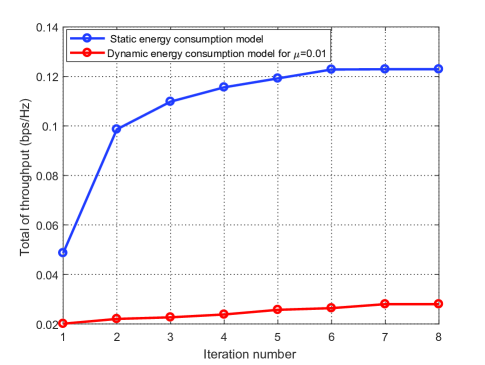
Figure 2: Convergence behaviour of Algorithm 1.

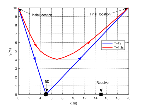
Figure 3: UAV trajectory obtained by our proposed scheme with static circuit power consumption cases.

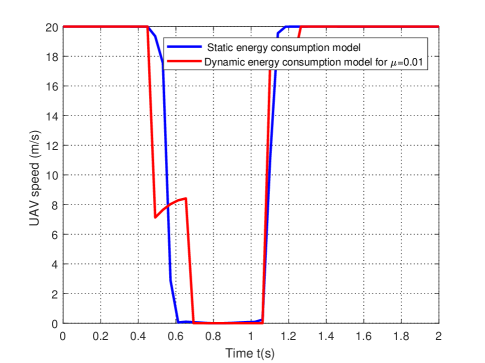
Figure 4: UAV speed calculated by our proposed scheme for the two circuit power consumption cases when $T=2{\rm s}$.

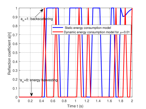
Figure 5: BD reflection coefficient for the two circuit power consumption cases when $T=2{\rm s}$.

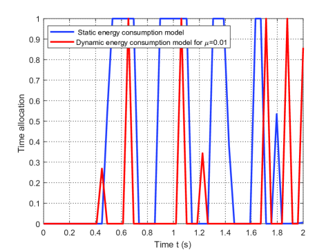
Figure 6: BD transmission time allocation for the two circuit power consumption cases when $T=2{\rm s}$.

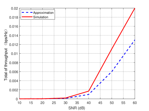
Figure 7: The impact of SNR on system performance based on approximation versus numerical result under period $T=2\rm s$ and $\mu=0.01$.

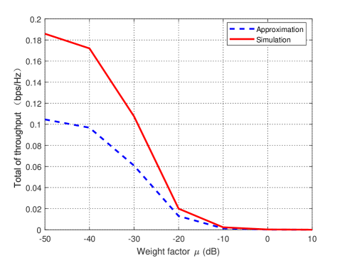
Figure 8: The impact of weight factor $\mu$ on system performance based on approximation versus numerical result under period $T=2\rm s$.

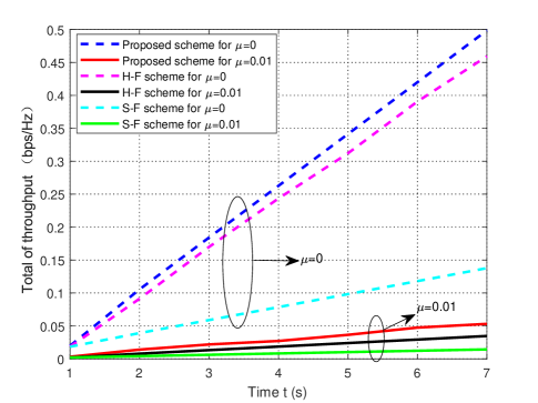
Figure 9: Total of throughput versus period $T$ for the two circuit power consumption cases with different optimization schemes.

V NUMERICAL RESULTS

In this section, numerical simulations are provided to evaluate the performance of our proposed schemes. The channel gain of the system is set to ${\beta_{0}}=-30{\rm{dB}}$ [11] [20], and the noise power at the UAV and receiver are assumed to be equal, $\sigma_{r}^{2}=\sigma_{u}^{2}=-90{\rm dB}$ [49]. The UAV altitude is fixed at ${H=10\rm{m}}$ with the maximum transmit power $P=1{\rm W}$ and maximum speed $V_{\rm max}=20{\rm{m/s}}$ [24], [49]. The duration of each time slot is $\delta=0.04\rm s$. The energy harvesting efficiency is assumed to be $\eta=0.9$, and the path loss coefficient is set to $m=3$ [24]. The BD’s circuit power consumption is in the order of micro-watt [13], [50], we set $P_{c}=10^{-5}\rm W$ and ${P_{\varepsilon}}=\frac{{{P_{c}}}}{{5}}$ without loss of generality. The step size $\pi$ is set to 0.01. The horizontal locations of the BD and receiver are respectively set to ${\bf w}_{b}=(5{\rm m},0)^{T}$ and ${\bf w}_{r}=(15{\rm m},0)^{T}$. The UAV’s initial and final location are ${\bf q}_{\rm I}=\left({0,10{\rm m}}\right)^{T}$ and ${\bf q}_{\rm F}=\left({20{\rm m},10{\rm m}}\right)^{T}$, respectively.

V-A Direct Link Available

We first consider the system model where the direct link between BD and receiver is available. In our initial setups, the initial trajectory for UAV is a straight path from the initial location to the final location with a steady speed, and the initial reflection coefficient for BD at any time slot $n$ is set to 0.5. In Fig. 2, we plot the convergence behaviour of Algorithm 1 for the static and dynamic circuit power consumption when $T=2\rm s$. It is observed that the throughput increases quickly and converges within a few iterations, which demonstrates the effectiveness of the Algorithm 1.

Fig. 3 shows the UAV trajectory obtained for the static circuit power consumption model for $T=2\rm s$ (the trajectory for the dynamic model is essentially identical and thus is omitted). We see that the UAV flies in a straight line to the BD, and then directly to the final location. The corresponding UAV speed for both circuit power models are plotted in Fig. 4. For the static model, we see that the UAV first flies with maximum speed towards the BD, hovers above the BD, and then flies with maximum speed from the BD to the final location. The UAV moves in the direction of the BD to improve the throughput, and has time to hover hear the BD before moving towards the final location. The maximum allowed hover time is constrained by the maximum UAV speed, the distance from the initial/final location to the BD, and the period $T$.

The optimized reflection coefficients for the two circuit power models are plotted in Fig. 5 for the case of for period $T=2\rm s$. A value of $a_{n}=0$ indicates that the BD only harvests energy from the UAV at time slot $n$, and no data is backscattered by the BD. In contrast, $a_{n}=1$ indicates that the BD transmits the data to receiver with maximum reflection coefficient , and no energy is harvested. It is observed that for the static circuit power model, the BD harvests energy first, and then uses the preserved energy for data transmission with maximum reflection coefficient. Interestingly, the duration for BD data backscattering for the static circuit power consumption model is significantly larger than the dynamic model. This is due to the fact that the dynamic model is more energy hungry than the static model, and as a consequence, more time needed to harvest energy from the UAV. In addition, the optimized time allocation for the BD is plotted in Fig. 6. When $a_{n}=1$ within period from $0.4\rm s$ to $1.7\rm s$ in Fig. 5, the entire time slot $n$ will be used for data backscattering for the static circuit power model as shown in Fig. 6. In contrast, for $a_{n}=0$, time slot $n$ will not be used for backscattering. Also, for the dynamic circuit power model, the BD’s backscattering time is much less than the static circuit power model case.

To evaluate the accuracy of the approximation of the expected throughput given in (14), the desired throughput given in (13) is compared. Fig. 7 shows the compared results for the different SNR under period $T=2\rm s$ and $\mu=0.01$. The value SNR is calculated as $\beta_{0}/\sigma_{r}^{2}$ with fixed ${\beta_{0}}=-30{\rm{dB}}$ and $\sigma_{r}^{2}$ varying from $-40{\rm dB}$ to $-90{\rm dB}$. For the approximation of the expected throughput, the results are obtained via Algorithm 1. For the desired throughput, the desired throughput is averaged over $10^{6}$ random channel realizations at each UAV location under $K=15\rm{dB}$. It is expected that the throughput is monotonically increasing with SNR for the approximation and simulation realizations. In addition, it also can be seen that for the small value SNR, namely $40{\rm{dB}}$, the obtained throughput for approximation is almost same as for numerical simulation. For the relatively large value SNR, the proposed optimization technique based on approximation may still be applied with an acceptable accuracy.

Fig. 8 shows the results of approximation and numerical simulations for the different weight factor $\mu$ under period $T=2\rm s$. First, it is observed that the system throughput degrades as $\mu$ increases for the approximation and numerical simulations. This is expected since a larger $\mu$ means more dynamical energy must be consumed, and hence the time allocation and reflection coefficient need to be smaller to satisfy the energy harvesting and circuit power consumption constraint. Second, for a very small weight factor with $\mu=-50\rm{dB}$, the approximation of the expected throughput of $0.11{\rm{bps/Hz}}$ is achieved. When the weight factor $\mu$ is higher than $-20\rm{dB}$, the approximation achieves a good accuracy with the numerical simulations.

In Fig. 9, to show the superiority of our proposed scheme, we compare it with the following benchmarks: 1) H-F scheme, where the BD forwards the data at time slot $n$ by using the harvested energy from time slot $n-1$. Mathematically, the constraint (23) is changed to ${\varphi_{2i}}P_{2i}^{e}\leq\eta\left({1-{a_{2i-1}}}\right)P\theta_{2i-1}^{ub},n\in{\cal N}_{1}$; 2) S-F scheme, where the UAV flies directly from the initial location to the final location in a straight line, but the time allocation and reflection coefficient are both optimized. It is observed that the static model results in a higher performance gain compared with the dynamic model for three schemes. This is expected since the higher transmission means more energy will be consumed, which thus degrades the system performance due to the energy budget constraint. In addition, the proposed scheme and the H-F scheme outperform the S-F scheme, which shows the advantage of optimizing the UAV trajectory in order to realize the full benefit of the UAV-aided backscatter communication.

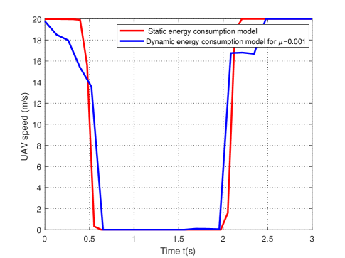
Figure 10: UAV speed obtained by our proposed scheme for the two circuit power consumption cases when $T=3{\rm s}$.

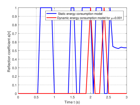
Figure 11: BD reflection coefficient for the two circuit power consumption cases when $T=3{\rm s}$.

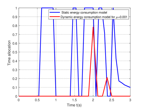
Figure 12: BD transmission time allocation for the two circuit power consumption cases when $T=3{\rm s}$.

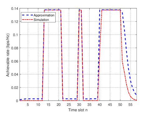
Figure 13: Approximation result based on (21) versus numerical simulation based on (18) under $\mu=0$, $K=15\rm dB$, and $T=7\rm s$.

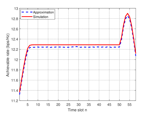
Figure 14: Approximation based on (22) versus numerical simulation based on (20) under $\mu=0$, $K=15\rm dB$, and $T=7\rm s$.

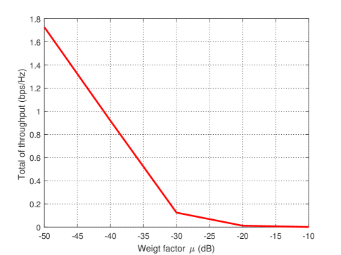
Figure 15: The impact of the weight factor $\mu$ on system performance for period $T=3\rm s$.

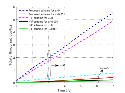
Figure 16: Total of throughput versus period $T$ for two circuit power consumption cases with different optimization schemes.

V-B Direct Link Unavailable

Next, we study the throughput maximization of the backscatter network when the direct link between BD and receiver is not available. Fig. 10 shows the UAV speed obtained by our proposed scheme for both the static and dynamic power models when $T=3\rm s$. The UAV trajectories for both models are nearly the same as the UAV trajectory plotted in Fig. 3. For the static power model in Fig. 10, the behavior of the UAV is the same as before, flying with maximum speed to the BD, hovering above the BD for as long as possible, then flying with maximum speed to the final location. This is expected since the longer the BD can be served, more energy can be harvested and the system throughput will increase. The result for the dynamic model is similar.

Figs. 11 and 12 show the reflection coefficient and time allocation obtained by our proposed schemes, respectively. For both circuit power models, the BD first harvests energy to the UAV and then reflects signal to the UAV. We can also see that the energy harvesting time for the dynamic circuit power model is larger than in the static model, which indicates that the dynamic model results in less time for BD data backscattering.

Fig. 13 and Fig. 14 compare the approximation of expected achievable rate and the numerical simulation of expected achievable rate under $\mu=0$, $K=15\rm dB$, and $T=7\rm s$. Fig. 13 first shows the results of achievable rate for approximation based on $R^{u}_{3n-1}$ in (21) and numerical simulation based on $\check{R}^{u}_{3n-1}$ in (18). It is observed from Fig. 13 that the approximation result $R^{u}_{3n-1}$ matches well with the numerical simulation result $\check{R}^{u}_{3n-1}$ at all time slot. Fig. 14 shows the results of achievable rate for approximation based on $R_{3n}^{r}$ in (22) and numerical simulation based on $\check{R}_{3n}^{r}$ in (20). It is observed from Fig. 14 that a satisfactory accuracy for approximation result $R_{3n}^{r}$ and numerical simulation result $\check{R}_{3n}^{r}$ is also obtained. In addition, comparing with Fig. 13 and Fig. 14, the value $R^{u}_{3n-1}$ shown in Fig. 13 is indeed much smaller than $R^{r}_{3n}$ shown in Fig. 14. This demonstrates the valid assumption of Remark 1. In addition, for the non-zero weight factor $\mu$, we can obtain similar result as in the case of $\mu=0$, and is omitted here for brevity.

Fig. 15 shows the impact of the weight factor $\mu$ on the system performance. The throughput is monotonically decreasing with the value $\mu$. For example, with a small value $\mu=-50\rm dB$, the throughput can achieve up to $1.76\rm bps/Hz$. However, when $\mu$ is larger than $\mu=-20\rm dB$, the system throughput is nearly to zero.

In Fig. 16, we compare the system throughput achieved by our proposed scheme with the other benchmarks for different values of $T$. We see that for $\mu=0$, our proposed scheme is superior to the H-F scheme and S-F scheme achieving higher throughput than the benchmarks. The performance gain becomes more substantial as $T$ grows. In addition, both the proposed scheme and H-F scheme outperform the S-F scheme, which indicates that optimization of the UAV trajectory significantly improves the system performance. Furthermore, it is observed that the schemes with static circuit power model for $\mu=0$ obtain a larger system throughput than the dynamic model for $\mu=0.001$.

VI Conclusion

This paper studied a UAV-aided BackCom network with and without a direct link between BD and receiver. Different static/dynamic circuit power consumption models for the two system models were considered. By exploiting the UAV mobility, the end-to-end achievable rate was maximized by jointly optimizing the time allocation, reflection coefficient and UAV trajectory. By means of the block coordinate descent and SCA techniques, an efficient iterative algorithm was proposed for both system models. The optimal time allocation for a given UAV trajectory under the static circuit power consumption model was derived in closed-form. In addition, for this case the optimal reflection coefficient was obtained with low computational complexity by using the Lagrangian dual method. Simulation results showed that the UAV mobility is beneficial for achieving a much higher system throughput than the other benchmarks that do not consider trajectory optimization. In addition, it was shown that more time will be used to backscatter for static circuit power consumption model compared with the dynamic circuit power consumption model, and results in much higher throughput than the dynamic model. Finally, it was shown that the proposed scheme significantly outperforms the H-F based scheme, thanks to the more degree of freedom for performance enhancement via careful energy harvesting and circuit power consumption design. The results in this paper can be further extended by considering following research directions: 1) The limited buffer size on BD; 2) Joint UAV trajectory and multiple access design for the multiple backscatter devices scenario; 3) The study of energy-efficient fixed/rotary wing UAV trajectory design by taking into account the UAV propulsion energy consumption.

Appendix A Proof of Theorem 1

To show Theorem 1, we first define the function $f\left(x\right){\rm{=}}{{\mathbb{E}}_{{X_{1}}{X_{2}}}}\left[{{{\log}_{2}}\left({1+{x_{1}}{x_{2}}}\right)}\right],({x_{1}},{x_{2}}>0)$, where $x_{1}$ and $x_{2}$ are independent with each other. We then have

$$f\left(x\right)\overset{a}{\leq}{\mathbb{E}_{{X_{1}}}}\left\{{\left[{{{\log}_{2}}\left({1+{x_{1}}{\mathbb{E}_{{X_{2}}}}\left[{{x_{2}}}\right]}\right)}\right]}\right\}=\mathord{\buildrel{\lower 3.0pt\hbox{$\scriptscriptstyle\frown$}}\over{f}}\left(x\right),$$ (54)

where inequality (a) in (54) holds due to the concavity of ${{{\log}_{2}}\left({1+{x_{1}}{x_{2}}}\right)}$ w.r.t. $x_{2}$ and Jensen’s inequality.

Based on the convexity of ${{{\log}_{2}}\left({1+e^{x}}\right)}$ w.r.t. $x$ and Jensen’s inequality, we have

$$\mathord{\buildrel{\lower 3.0pt\hbox{$\scriptscriptstyle\frown$}}\over{f}}\left(x\right) ={\mathbb{E}_{{X_{1}}}}\left[{{{\log}_{2}}\left({1+{x_{1}}{\mathbb{E}_{{X_{2}}}}\left[{{x_{2}}}\right]}\right)}\right]$$

$$={\mathbb{E}_{{X_{1}}}}\left[{{{\log}_{2}}\left({1+{\mathbb{E}_{{X_{2}}}}\left[{{x_{2}}}\right]{e^{\ln{x_{1}}}}}\right)}\right]$$

$$\geq{\log_{2}}\left({1+{\mathbb{E}_{{X_{2}}}}\left[{{x_{2}}}\right]{e^{{\mathbb{E}_{{X_{1}}}}\left[{\ln{x_{1}}}\right]}}}\right)=\hat{f}\left(x\right).$$ (55)

We should point out that $\hat{f}\left(x\right)$ is neither a upper bound result nor a lower bound result for $\mathord{\buildrel{\lower 3.0pt\hbox{$\scriptscriptstyle\frown$}}\over{f}}\left(x\right)$. Instead, $\hat{f}\left(x\right)$ is served as an approximation result for $\mathord{\buildrel{\lower 3.0pt\hbox{$\scriptscriptstyle\frown$}}\over{f}}\left(x\right)$. Letting ${x_{1}}=\frac{{P{a_{n}}{h_{br}}}}{{\sigma_{r}^{2}}}$ and ${x_{2}}=h_{n}^{ub}$, we have

$${\mathbb{E}_{{X_{2}}}}\left[{{x_{2}}}\right]{\rm{=}}\mathbb{E}\left[{\theta_{n}^{ub}{{\|{\tilde{h}_{n}^{ub}}\|}^{2}}}\right]{\rm{=}}\frac{{{\beta_{0}}}}{{{{\left\|{{{\bf{q}}_{n}}-{{\bf{w}}_{f}}}\right\|}^{2}}+{H^{2}}}}$$ (56)

and

$${\mathbb{E}_{{X_{1}}}}\left[{\ln{x_{1}}}\right]=\ln\frac{{P{a_{n}}{\beta_{0}}d_{br}^{-m}}}{{\sigma_{r}^{2}}}+\mathbb{E}\left[{\ln\xi}\right]=\ln\frac{{P{a_{n}}{\beta_{0}}d_{br}^{-m}}}{{\sigma_{r}^{2}}}-{\kappa_{0}},$$ (57)

where ${\kappa_{0}}$ is the Euler constant, $\mathbb{E}\left[{\ln\xi}\right]$ is derived from eq.(4.331.1) in [51]. Substituting (56) and (57) into $\hat{f}\left(x\right)$, we can easily obtain $\hat{R}^{r}_{n+1}$ in (14). This completes the proof of Theorem 1.

Appendix B Proof of Theorem  2

We first observe that problem $(\rm P1.1)$ is a linear optimization problem. Meanwhile, it can be verified that $(\rm P1.1)$ satisfies Slater’s condition, and thus the dual gap is zero and the optimal solution can be obtained by solving its dual problem [42]. Let ${\lambda_{n}}>0$ for $n=1,...,N/2$ be the Lagrangian dual variables corresponding to (23). The corresponding partial Lagrangian for problem $(\rm P1)$ can be expressed as

$${\cal L}\left({{\varphi_{2n}},{\lambda_{n}}}\right)=\sum\limits_{n=1}^{N/2}{{\varphi_{2n}}\hat{R}_{2n}^{r}}+$$

$$\sum\limits_{n=1}^{N/2}{{\lambda_{n}}\left({\sum\limits_{i=1}^{n}{\eta\left({1-{a_{2i-1}}}\right)}P\theta_{2i-1}^{ub}-\sum\limits_{i=1}^{n}{{\varphi_{2i}}{P_{c}}}}\right)}.$$ (58)

The KKT conditions are sufficient to obtain the optimal solution, and the partial conditions are given by

$$\frac{{\partial{\cal L}\left({\varphi_{2n}^{*},\lambda_{n}^{*}}\right)}}{{\partial\varphi_{2n}^{*}}}=0,$$ (59)

$$\lambda_{n}^{*}\left({\sum\limits_{i=1}^{n}{\eta\left({1-{a_{2i-1}}}\right)}P\theta_{2i-1}^{ub}-\sum\limits_{i=1}^{n}{\varphi_{2i}^{*}{P_{c}}}}\right)=0.$$ (60)

From equation (59), the optimal dual variables can be obtained as

$$\lambda_{n}^{*}=\frac{{\hat{R}_{2n}^{r}-\hat{R}_{2n+2}^{r}}}{{{P_{c}}}},n=1,...,N/2-1$$

$$\lambda_{N/2}^{*}=\frac{{\hat{R}_{N}^{r}}}{{{P_{c}}}}.$$ (61)

If ${\hat{R}_{2n}^{r}}$ is a decreasing function with $n\in{\cal N}_{1}$, the optimal value is positive, i.e., $\lambda_{n}^{*}>0$ for $n=1,...,N/2$. Based on the complementary slackness condition from (60), we must have

$$\sum\limits_{i=1}^{n}{\eta\left({1-{a_{2i-1}}}\right)}P\theta_{2i-1}^{ub}-\sum\limits_{i=1}^{n}{\varphi_{2i}^{*}{P_{c}}}=0,n\in{{\cal N}_{1}}.$$ (62)

Then, with (25) and (62), the optimal time allocation $\varphi_{2n}$ can be readily obtained in (30). This completes the proof of Theorem 2

Appendix C Proof of Lemma  1

Similar to Appendix B, let ${\nu_{n}}>0$ for $n=1,...,N/2$ be the Lagrangian dual variables corresponding to (23). The corresponding partial Lagrangian for problem $(\rm P1.2)$ can be expressed as

$${\cal L}\left({{a_{2n-1}},{\nu_{n}}}\right)=\sum\limits_{n=1}^{N/2}{{\varphi_{2n}}\hat{R}_{2n}^{r}}+$$

$$\sum\limits_{n=1}^{N/2}{{\nu_{n}}\left({\sum\limits_{i=1}^{n}{\eta\left({1-{a_{2i-1}}}\right)}P\theta_{2i-1}^{ub}-\sum\limits_{i=1}^{n}{{\varphi_{2i}}{P_{c}}}}\right)}.$$ (63)

Accordingly, the dual function for $(\rm P1)$ is given by

$$g\left({{v_{n}}}\right)=\left\{\begin{array}[]{l}\mathop{\max}\limits_{a_{2n-1}}{\cal L}\left({a_{2n-1},{v_{n}}}\right)\\ \quad{\rm s.t.}~{}\eqref{Case1_constr3}.\end{array}\right.$$ (66)

By applying the first order derivative of (63) w.r.t $a_{2n-1}$ and setting it to zero,, we have

$$\frac{{{W_{br}}{\varphi_{2n}}}}{{\ln 2\left({{{\left\|{{{\bf{q}}_{2n-1}}-{{\bf{w}}_{b}}}\right\|}^{2}}+{H^{2}}}\right)+{W_{br}}{a_{2n-1}}}}$$

$$\qquad\qquad\qquad\qquad\qquad\qquad-\eta P\theta_{2n-1}^{ub}\sum\limits_{i=n}^{N/2}{{\nu_{i}}}=0.$$ (67)

Then, the formula (33) can be readily obtained based on (24) and (67). This completes the proof of Lemma 1.

References

- [1] M. Hua, A. L. Swindlehurst, C. Li, and L. Yang, “UAV-aided backscatter networks: Joint UAV trajectory and protocol design,” in IEEE Global Communications Conference (GLOBECOM), accepted, 2019.
- [2] L. Xie, J. Xu, and R. Zhang, “Throughput maximization for UAV-enabled wireless powered communication networks - invited paper,” in 2018 IEEE 87th Vehicular Technology Conference (VTC Spring), 2018.
- [3] Q. Wu, W. Chen, D. W. K. Ng, and R. Schober, “Spectral and energy-efficient wireless powered IoT networks: NOMA or TDMA?” IEEE Transactions on Vehicular Technology, vol. 67, no. 7, pp. 6663–6667, 2018.
- [4] H. Ju and R. Zhang, “Throughput maximization in wireless powered communication networks,” IEEE Transactions on Wireless Communications, vol. 13, no. 1, pp. 418–428, 2014.
- [5] S. Bi, Y. Zeng, and R. Zhang, “Wireless powered communication networks: An overview,” IEEE Wireless Communications, vol. 23, no. 2, pp. 10–18, 2016.
- [6] S. Bi, C. K. Ho, and R. Zhang, “Wireless powered communication: Opportunities and challenges,” IEEE Communications Magazine, vol. 53, no. 4, pp. 117–125, 2015.
- [7] Y. Zeng, B. Clerckx, and R. Zhang, “Communications and signals design for wireless power transmission,” IEEE Transactions on Communications, vol. 65, no. 5, pp. 2264–2290, 2017.
- [8] J. Xu and R. Zhang, “Comp meets smart grid: A new communication and energy cooperation paradigm,” IEEE Transactions on Vehicular Technology, vol. 64, no. 6, pp. 2476–2488, 2015.
- [9] B. Lyu, C. You, Z. Yang, and G. Gui, “The optimal control policy for RF-powered backscatter communication networks,” IEEE Transactions on Vehicular Technology, vol. 67, no. 3, pp. 2804–2808, 2018.
- [10] X. Kang, Y.-C. Liang, and J. Yang, “Riding on the primary: A new spectrum sharing paradigm for wireless-powered IoT devices,” IEEE Transactions on Wireless Communications, vol. 17, no. 9, pp. 6335–6347, 2018.
- [11] B. Lyu, Z. Yang, H. Guo, F. Tian, and G. Gui, “Relay cooperation enhanced backscatter communication for internet-of-things,” IEEE Internet of Things Journal, 2018, to appear.
- [12] D. T. Hoang, D. Niyato, P. Wang, D. I. Kim, and Z. Han, “Ambient backscatter: A new approach to improve network performance for RF-powered cognitive radio networks,” IEEE Transactions on Communications, vol. 65, no. 9, pp. 3659–3674, 2017.
- [13] V. Liu, A. Parks, V. Talla, S. Gollakota, D. Wetherall, and J. R. Smith, “Ambient backscatter: wireless communication out of thin air,” in ACM SIGCOMM Computer Communication Review, vol. 43, no. 4. ACM, 2013, pp. 39–50.
- [14] B. Lyu, Z. Yang, G. Gui, and Y. Feng, “Wireless powered communication networks assisted by backscatter communication,” IEEE Access, vol. 5, pp. 7254–7262, 2017.
- [15] C. Boyer and S. Roy, “Backscatter communication and RFID: Coding, energy, and MIMO analysis,” IEEE Transactions on Communications, vol. 62, no. 3, pp. 770–785, 2014.
- [16] ——, “Space time coding for backscatter RFID,” IEEE Transactions on Wireless Communications, vol. 12, no. 5, pp. 2272–2280, 2013.
- [17] A. N. Parks, A. P. Sample, Y. Zhao, and J. R. Smith, “A wireless sensing platform utilizing ambient RF energy,” in 2013 IEEE Topical Conference on Biomedical Wireless Technologies, Networks, and Sensing Systems. IEEE, 2013, pp. 154–156.
- [18] B. Lyu, H. Guo, Z. Yang, and G. Gui, “Throughput maximization for hybrid backscatter assisted cognitive wireless powered radio networks,” IEEE Internet of Things Journal, vol. 5, no. 3, pp. 2015–2024, 2018.
- [19] X. Wang, Z. Su, and G. Wang, “Relay selection for secure backscatter wireless communications,” Electronics Letters, vol. 51, no. 12, pp. 951–952, 2015.
- [20] J. Xu, Y. Zeng, and R. Zhang, “UAV-enabled wireless power transfer: Trajectory design and energy optimization,” IEEE Transactions on Wireless Communications, vol. 17, no. 8, pp. 5092–5106, 2018.
- [21] C. Zhan, Y. Zeng, and R. Zhang, “Energy-efficient data collection in UAV enabled wireless sensor network,” IEEE Wireless Communications Letters, vol. 7, no. 3, pp. 328–331, 2018.
- [22] H. Wang, G. Ding, F. Gao, J. Chen, J. Wang, and L. Wang, “Power control in UAV-supported ultra dense networks: Communications, caching, and energy transfer,” IEEE Communications Magazine, vol. 56, no. 6, pp. 28–34, 2018.
- [23] Y. Zeng, R. Zhang, and T. J. Lim, “Wireless communications with unmanned aerial vehicles: Opportunities and challenges,” IEEE Communications Magazine, vol. 54, no. 5, pp. 36–42, 2016.
- [24] J. Lyu, Y. Zeng, and R. Zhang, “UAV-aided offloading for cellular hotspot,” IEEE Transactions on Wireless Communications, vol. 17, no. 6, pp. 3988–4001, 2018.
- [25] Y. Zeng, R. Zhang, and T. J. Lim, “Throughput maximization for UAV-enabled mobile relaying systems,” IEEE Transactions on Communications, vol. 64, no. 12, pp. 4983–4996, 2016.
- [26] M. Hua, Y. Wang, M. Lin, C. Li, Y. Huang, and L. Yang, “Joint CoMP transmission for UAV-aided cognitive satellite terrestrial networks,” IEEE Access, vol. 7, pp. 14 959–14 968, 2019.
- [27] Q. Wu, Y. Zeng, and R. Zhang, “Joint trajectory and communication design for multi-UAV enabled wireless networks,” IEEE Transactions on Wireless Communications, vol. 17, no. 3, pp. 2109–2121, 2018.
- [28] F. Jiang and A. L. Swindlehurst, “Optimization of UAV heading for the ground-to-air uplink,” IEEE Journal on Selected Areas in Communications, vol. 30, no. 5, pp. 993–1005, 2012.
- [29] Z. Han, A. L. Swindlehurst, and K. R. Liu, “Optimization of MANET connectivity via smart deployment/movement of unmanned air vehicles,” IEEE Transactions on Vehicular Technology, vol. 58, no. 7, pp. 3533–3546, 2009.
- [30] P. Zhan, K. Yu, and A. L. Swindlehurst, “Wireless relay communications with unmanned aerial vehicles: Performance and optimization,” IEEE Transactions on Aerospace and Electronic Systems, vol. 47, no. 3, pp. 2068–2085, 2011.
- [31] M. Hua, Y. Wang, Z. Zhang, C. Li, Y. Huang, and L. Yang, “Power-efficient communication in UAV-aided wireless sensor networks,” IEEE Communications Letters, vol. 22, no. 6, pp. 1264–1267, 2018.
- [32] Y. Zeng and R. Zhang, “Energy-efficient UAV communication with trajectory optimization,” IEEE Transactions on Wireless Communications, vol. 16, no. 6, pp. 3747–3760, 2017.
- [33] H. Wang, J. Wang, G. Ding, J. Chen, Y. Li, and Z. Han, “Spectrum sharing planning for full-duplex UAV relaying systems with underlaid D2D communications,” IEEE Journal on Selected Areas in Communications, vol. 36, no. 9, pp. 1986–1999, 2018.
- [34] L. Xie, J. Xu, and R. Zhang, “Throughput maximization for UAV-enabled wireless powered communication networks,” IEEE Internet of Things Journal, 2018, to appear.
- [35] D. W. Matolak and R. Sun, “Unmanned aircraft systems: Air-ground channel characterization for future applications,” IEEE Vehicular Technology Magazine, vol. 10, no. 2, pp. 79–85, 2015.
- [36] A. A. Khuwaja, Y. Chen, N. Zhao, M.-S. Alouini, and P. Dobbins, “A survey of channel modeling for UAV communications,” IEEE Communications Surveys & Tutorials, vol. 20, no. 4, pp. 2804–2821, 2018.
- [37] C. You and R. Zhang, “3D trajectory optimization in rician fading for UAV-enabled data harvesting,” IEEE Transactions on Wireless Communications, vol. 18, no. 6, pp. 3192–3207, 2019.
- [38] N. Ahmed, S. S. Kanhere, and S. Jha, “On the importance of link characterization for aerial wireless sensor networks,” IEEE Communications Magazine, vol. 54, no. 5, pp. 52–57, 2016.
- [39] Y. Zeng, Q. Wu, and R. Zhang, “Accessing from the sky: A tutorial on UAV communications for 5g and beyond,” Proceedings of the IEEE, Editor Invited Paper, Submitted, 2019. https://arxiv.org/abs/1903.05289.
- [40] G. Wang, F. Gao, R. Fan, and C. Tellambura, “Ambient backscatter communication systems: Detection and performance analysis,” IEEE Transactions on Communications, vol. 64, no. 11, pp. 4836–4846, 2016.
- [41] J. Qian, F. Gao, G. Wang, S. Jin, and H. Zhu, “Noncoherent detections for ambient backscatter system,” IEEE Transactions on Wireless Communications, vol. 16, no. 3, pp. 1412–1422, 2017.
- [42] S. Boyd and L. Vandenberghe, Convex optimization. Cambridge university press, 2004.
- [43] A. A. Nasir, X. Zhou, S. Durrani, and R. A. Kennedy, “Relaying protocols for wireless energy harvesting and information processing,” IEEE Transactions on Wireless Communications, vol. 12, no. 7, pp. 3622–3636, 2013.
- [44] M. Grant, S. Boyd, and Y. Ye, “CVX: Matlab software for disciplined convex programming,” 2008.
- [45] W. Yu and R. Lui, “Dual methods for nonconvex spectrum optimization of multicarrier systems,” IEEE Transactions on Communications, vol. 54, no. 7, pp. 1310–1322, 2006.
- [46] Q. Wu, W. Chen, M. Tao, J. Li, H. Tang, and J. Wu, “Resource allocation for joint transmitter and receiver energy efficiency maximization in downlink OFDMA systems,” IEEE Transactions on Communications, vol. 63, no. 2, pp. 416–430, 2015.
- [47] J. Gondzio and T. Terlaky, “A computational view of interior point methods,” JE Beasley. Advances in linear and integer programming. Oxford Lecture Series in Mathematics and its Applications, vol. 4, pp. 103–144, 1996.
- [48] G. Zhang, Q. Wu, M. Cui, and R. Zhang, “Securing uav communications via joint trajectory and power control,” IEEE Transactions on Wireless Communications, vol. 18, no. 2, pp. 1376–1389, 2019.
- [49] F. Zhou, Y. Wu, R. Q. Hu, and Y. Qian, “Computation rate maximization in UAV-enabled wireless-powered mobile-edge computing systems,” IEEE Journal on Selected Areas in Communications, vol. 36, no. 9, pp. 1927–1941, 2018.
- [50] V. Iyer, V. Talla, B. Kellogg, S. Gollakota, and J. Smith, “Inter-technology backscatter: Towards internet connectivity for implanted devices,” in Proceedings of the 2016 ACM SIGCOMM Conference. ACM, 2016, pp. 356–369.
- [51] I. S. Gradshteyn and I. M. Ryzhik, Table of integrals, series, and products. Seventh Edition,San Diego, CA: Academic press, 2014.