High order ADER schemes for continuum mechanics

Abstract

In this paper we first review the development of high order ADER finite volume and ADER discontinuous Galerkin schemes on fixed and moving meshes, since their introduction in 1999 by Toro et al. We show the modern variant of ADER based on a space-time predictor-corrector formulation in the context of ADER discontinuous Galerkin schemes with a posteriori subcell finite volume limiter on fixed and moving grids, as well as on space-time adaptive Cartesian AMR meshes. We then present and discuss the unified symmetric hyperbolic and thermodynamically compatible (SHTC) formulation of continuum mechanics developed by Godunov, Peshkov and Romenski (GPR model), which allows to describe fluid and solid mechanics in one single and unified first order hyperbolic system. In order to deal with free surface and moving boundary problems, a simple diffuse interface approach is employed, which is compatible with Eulerian schemes on fixed grids as well as direct Arbitrary-Lagrangian-Eulerian methods on moving meshes. We show some examples of moving boundary problems in fluid and solid mechanics.

1 Introduction and review of the ADER approach

The development of high order numerical schemes for hyperbolic conservation laws has been one of the major challenges of numerical analysis for the last decades. [101] proved that for the linear advection equation no monotone linear schemes of second or higher order of accuracy can be constructed. Therefore, even if physical viscosity is considered, a linear high order scheme will present spurious oscillations near discontinuities, as it can be seen, for instance for the Lax-Wendroff scheme, [128]. A first idea to circumvent this theorem has been proposed in [127], where limited slopes are employed to produce a non-linear scheme of second order of accuracy in space. Since then, many high order numerical methods have been developed like the Total Variation Disminishing methods (TVD) and Flux limiter methods (see, for instance, [109, 170, 104, 189, 190, 176]). Despite these methodologies being already well established at the end of the last century, their major drawback was that they just provided global second order of accuracy and reduced locally to first order in the vicinity of smooth extrema.

More advanced non-linear methods for advection dominated problems involve the family of ENO and WENO schemes, see [111, 110, 165]. In particular, the method of [110] is a fully discrete high order scheme that can be re-interpreted in terms of the solution of a generalized Riemann problem (GRP), see [41]. Moreover, it can be seen as a generalization of the MUSCL-Hancock method of van Leer, see [190, 176, 16].

Following the idea of solving a generalized Riemann problem (GRP), see also [13, 129, 15, 106], the ADER approach (Arbitrary high order DErivative Riemann problem) has been first put forward for the linear advection equation with constant coefficients by [140, 178]. The first step of the methodology involves piece-wise polynomial data reconstruction, where a nonlinear ENO reconstruction is applied in order to avoid spurious oscillations of the numerical solution. Then, a GRP is defined at each cell interface. Classically, the initial condition for the GRP was given as piece-wise linear polynomials and second order schemes could be obtained by constructing a space-time integral of the solution in an appropriate control volume [182, 17], or following a MUSCL approach, [188, 47]. An alternative methodology proposed in [14] consists in expressing the solution of the GRP as a Taylor series expansion in time. The ADER approach obtains the high order time derivatives of the GRP solution at the cell interface via the Cauchy-Kovalevskaya procedure, which replaces time derivatives by spatial derivatives using repeated differentiation of the differential form of the PDE. The spatial derivatives, which may also jump at the interface, are defined via the solution of linearized Riemann problems for the derivatives, where linearization is carried out about the Godunov state obtained from the classical Riemann problem between the boundary extrapolated values at the interface. In Figure 1, the classical piece-wise constant polynomials are plotted against a high order reconstruction and the similarity solutions for both cases are sketched. Finally, these similarity solutions are used to construct the numerical flux. The resulting schemes are arbitrary high order accurate in both space and time, in the sense that they have no theoretical accuracy barrier.

Figure 1: Classical piece-wise reconstruction polynomials used in the ADER approach, $p_{i}(x)$ and $p_{i+1}(x)$, and the structure of the Riemann problem solution at the intercell boundary $x_{i+\frac{1}{2}}$. Left: classical piece-wise constant data. Right: piece-wise smooth reconstruction.

Since their introduction in [178, 140], many extensions of the ADER methodology have been proposed. Regarding 2D linear PDEs, one may refer to [163] and their simplification for the particular case of structured grids in [162]. Moreover, non linear systems have been initially addressed in [180, 174]. Further applications of ADER on non-Cartesian meshes have been presented in [125, 124, 71, 41]. One should also mention the development of ADER schemes in the framework of discontinuous Galerkin (DG) finite element methods, see [152, 74, 94]. One of the main advantages of using DG is that the reconstruction step of classical ADER finite volume (ADER-FV) schemes can be skipped, since the discrete solution is already given by high order piecewise polynomials that can be directly evolved during each time step. Furthermore, ADER-DG schemes avoid the use of classical Runge-Kutta time stepping and thus provide efficient communication-avoiding schemes for parallel computing, see [82] and allow for simple and natural time-accurate local time stepping (LTS), see [72].

An important step forward in the development of more general ADER schemes was achieved in [64], where a new class of ADER-FV methods has been introduced. The main contribution of this paper consists in the introduction of a new element-local space-time DG predictor, which allows at the same time the treatment of stiff source terms, as well as the replacement of the cumbersome Cauchy-Kovalevskaya procedure. First, a high order WENO method is employed to compute a polynomial reconstruction of the data inside each spatial element; then, an element-local weak formulation of the conservation law is considered in space-time and the predictor is applied to construct the time evolution of the WENO polynomials within each cell. Note that, in this step, the integration by parts is performed only in time, which differs from global space-time DG schemes [186, 187], which are globally implicit. Finally, the cell averages are updated with an explicit fully discrete one-step scheme, considering the integral form of the equations. As a result, the proposed methodology maintains arbitrary high order of accuracy, while avoiding the issues related to the use of a Taylor series expansion in time. As already mentioned above, it naturally provides an approach for the treatment of stiff source terms (for further details on this topic, see [112] and references therein).

The above methodology can also be applied in the discontiuous Galerkin framework as presented in [61], where, a unified $P_{N}P_{M}$ framework for arbitrary high order one-step finite volume and DG schemes has been introduced. For other reconstruction-based DG schemes, see e.g. [136, 137]. Afterwards, the methodology has been extended to solve a wide variety of different PDE systems, such as the resistive relativistic MHD equations, [79]; non conservative hyperbolic systems found in geophysical flows, [63] in which a well-balanced and path-conservative version of the scheme has been developed; compressible multi-phase flows [68], the compressible Navier-Stokes equations, [58]; the compressible Euler equations and divergence-free schemes for MHD, [6, 5], where ADER schemes were used in combination with genuinely multidimensional Riemann solvers. The last extensions concern the special and general relativistic MHD equations, see [192, 82], as well as the Einstein field equations of general relativity [67, 65].

Later, ADER schemes have been extended to adaptive mesh refinement on Cartesian grids (AMR), in combination with time accurate local time stepping (LTS). This technique has initially been introduced in [80, 69] for conservative and non-conservative hyperbolic systems, respectively. Moreover, the schemes of the ADER family were the first high order methods to be applied for the numerical solution of the unified first order hyperbolic formulation of continuum mechanics by Godunov, Peshkov and Romenski [103, 150, 100], see [76, 77, 66]. In the rest of this paper, we will refer to the Godunov-Peshkov-Romenski model of continuum mechanics as GPR model.

The ADER approach has also been extended to the direct Arbitrary-Lagrangian-Eulerian framework (ALE), where the mesh moves with an arbitrary velocity, taken as close as possible to the local fluid velocity. Initially developed for one space dimension, it has been soon extended to the case of the two and three dimensional Euler equations on unstructured meshes, [21, 22], including the discretization of non-conservative products. Further works in this area involve the use of local timestepping techniques, [60, 29]; coupling with multidimensional HLL Riemann solvers, [20]; solution of magnetohydrodynamics problems (MHD), [18, 26]; development of a quadrature-free approach to increase the computational efficiency of the overall method, [23]; use of curvilinear unstructured meshes, [24]; or extension to solve the GPR model, [27, 148]. Furthermore, in [93] a novel algorithm to deal with moving nonconforming polygonal grids has been presented. The methodology reduces the typical mesh distortion arising in shear flows and provides high quality elements even for long-time simulations. An exactly well-balanced path-conservative version of this approach for the Euler equations with gravity can be found in [92]. Still in the ALE framework, within this article, we will present new results for the family of ADER-FV and ADER-DG schemes on moving unstructured Voronoi meshes [168], as recently introduced in [89, 90].

It is well known that when dealing with high order schemes special care must be paid to the limiting methodology employed. In most of the previous referenced papers classical a priori limiters have been used, such as WENO reconstruction. Nevertheless, some alternative contributions to this topic can be found in the series of papers [81, 135, 193, 73, 192, 19, 30, 83, 173, 90], where a novel a posteriori sub-cell FV limiter of high order DG schemes, based on the MOOD paradigm of [45, 55, 56], has been employed.

Besides the references given above, which focus on the development of the ADER methodology with a local space-time Galerkin predictor, many recent papers have been devoted to the development of other families of ADER schemes, like the classical ADER finite volume methods. Without pretending to be exhaustive, we may refer to [40, 177, 171, 176, 141, 143, 184, 179, 183, 35, 142, 38, 48, 36, 53] and references therein.

In this paper, as a promising application of the family of ADER schemes, we solve a diffuse interface formulation of the GPR model of continuum mechanics. In comparison with existing continuum mechanics models, the novel feature of the GPR model is in that it incorporates the two main branches of continuum mechanics, fluid and solid mechanics, in one single unified PDE system. Recall that traditionally fluid and solid mechanics are described by PDE systems of different types, i.e. parabolic (viscous fluids) and hyperbolic (linear elasticity and hyperelasticity), which imposes many theoretical and technical difficulties if one wishes to model natural and industrial processes involving co-existence of the fluid and solid states such as in fluid-structure interaction (FSI) problems, modeling of general solid-fluid transition such as in melting and solidification processes, e.g. additive manufacturing, see for example [87], flows of granular media [2], viscoplastic flows, e.g. debris flows, avalanches, mantle convection, flows of many industrial Bingham-type fluids, see [3]. Due to the unified treatment of fluids and solids, the GPR model thus has a great potential for simplifying the modeling process and code development for solving the aforementioned problems. Yet, before to be applied to practical problems, the GPR model may require a coupling with an interface tracking/capturing technique for the modeling of moving material boundaries such as in free surface flows or solid body motion. In particular, in this paper, we couple the GPR model with a simple diffuse interface approach, see [173, 59, 91, 126]. For example, very interesting computational results with similar diffuse interface approaches and level set techniques for compressible multi-material flows have been obtained for example in [95, 85, 84, 144, 51, 139, 119, 12]. Finally, we demonstrate that the ADER family of schemes is capable to resolve the GPR model in both solid and fluid regimes.

The paper is organized as follows. In Section 2 we present the family of ADER finite volume and ADER discontinuous Galerkin finite element schemes on fixed Cartesian and moving polygonal meshes in two space dimensions. Next, in Section 3 we introduce the diffuse interface formulation of the GPR model. In Section 4 we show some computational results obtained with different kinds of ADER schemes (ADER-FV and ADER-DG) on different mesh topologies, including moving unstructured Voronoi meshes, as well as fixed and adaptive Cartesian grids. The paper is rounded off by some concluding remarks and an outlook to future work in Section 5.

2 ADER finite volume and discontinuous Galerkin schemes

The numerical method adopted in this paper is the variant of the arbitrary high-order accurate ADER approach based on the space-time predictor-corrector formalism, which we have briefly reviewed in the previous Section 1. It easily applies to the context of finite volume (FV) and discontinous Galerkin (DG) methods, using either space-time adaptive Cartesian grids (AMR), see [33, 191, 80, 193, 83, 82] and references therein, or unstructured meshes, and both on fixed Eulerian domains or in a moving Arbitrary-Lagrangian-Eulerian (ALE) framework, see [29, 26, 21, 22, 25, 19, 88, 90] and references therein.

Here, we briefly describe the key features of our numerical scheme, keeping the notation as general as possible, and referring to the literature for further details. We start by introducing the general form of our governing PDE system and a moving unstructured discretization of two-dimensional domains (Sections 2.1 and 2.2); next, in Section 2.3 we describe the data representation of the discrete solution. Then, we explain how to obtain high order of accuracy in space: this is available by construction in the DG case, and obtained via some variants of the well known WENO procedure ([120, 7, 71, 70, 194, 166]) for the FV approach. Finally, we focus on the predictor-corrector version of the ADER scheme that allows to achieve arbitrary high order of accuracy in space and time. Since it is out of the scope of this paper to recall all the details, a general overview is given in Sections 2.5 and 2.7, and an inedited proof of the convergence of the predictor for a nonlinear conservation law is presented in Section 2.6.

We would like to emphasize that, besides this novel convergence proof, other progress has been introduced within this work. Indeed, up to our knowledge, it is the first time that: (i) the ADER approach is used to solve a diffuse interface formulation of the GPR model that addresses the free surface problem in both solid and fluid mechanics context (previously, a similar formulation was used only in the solid dynamics context [108, 107, 145]); (ii) non-conservative products are taken into account in the high order direct ALE scheme of [90], where they have to be integrated also on degenerate space–time control volumes (see Section 2.5).

2.1 Governing PDE system

In this paper we consider high order fully-discrete schemes for nonlinear systems of hyperbolic PDE with non-conservative products and algebraic source terms of the form

$$\frac{\partial\mathbf{Q}}{\partial t}+\nabla\cdot\mathbf{F}\left(\mathbf{Q}\right)+\mathbf{B}(\mathbf{Q})\cdot\nabla\mathbf{Q}=\mathbf{S}(\mathbf{Q}),$$ (1)

where $\mathbf{Q}=\mathbf{Q}(\mathbf{x},t)\in\Omega_{Q}\subset\mathbb{R}^{m}$ is the state vector, $t\in\mathbb{R}_{0}^{+}$ is the time, $\mathbf{x}\in\Omega\subset\mathbb{R}^{d}$ is the spatial coordinate, $d$ is the number of space dimensions, $\Omega_{Q}$ is the so-called state space or phase space, $\mathbf{F}(\mathbf{Q})$ is the nonlinear flux tensor, $\mathbf{B}(\mathbf{Q})\cdot\nabla\mathbf{Q}$ is a non-conservative product and $\mathbf{S}(\mathbf{Q})$ is a purely algebraic source term. Introducing the system matrix $\mathbf{A}(\mathbf{Q})=\partial\mathbf{F}/\partial\mathbf{Q}+\mathbf{B}(\mathbf{Q})$ the above system can also be written in quasi-linear form as

$$\frac{\partial\mathbf{Q}}{\partial t}+\mathbf{A}(\mathbf{Q})\cdot\nabla\mathbf{Q}=\mathbf{S}(\mathbf{Q}).$$ (2)

The system is said to be hyperbolic if for all $\mathbf{n}\neq 0$ and for all $\mathbf{Q}\in\Omega_{Q}$ the matrix $\mathbf{A}(\mathbf{Q})\cdot\mathbf{n}$ has $m$ real eigenvalues and a full set of $m$ linearly independent right eigenvectors. The system (1) needs to be provided with an initial condition $\mathbf{Q}(\mathbf{x},0)=\mathbf{Q}_{0}(\mathbf{x})$ and appropriate boundary conditions on $\partial\Omega$.

In this paper we focus on a particular, but very general, example of a first-order system (1) describing elastic and visco-plastic heat-conducting media; it will be discussed in Section 3.

2.2 Domain discretization

In the general ALE case, we consider a moving two-dimensional $(d=2)$ domain $\Omega(t)$ and we cover it using an unstructured mesh made of $N_{P}$ non overlapping polygons $P_{i},i=1,\dots N_{P}$. The mesh is first built at time $t=0$ and then it is rearranged at each time step $t^{n}$: elements and nodes are moved following the local fluid velocity and when necessary, in order to prevent mesh distortion, also the mesh topology (i.e. the shape of the elements and their connectivities) is changed.

Given a polygon $P_{i}^{n}$ we denote by $\mathcal{V}(P_{i}^{n})=\{v_{i_{1}}^{n},\dots,v_{i_{j}}^{n},$ $\dots,v_{i_{N_{V_{i}}^{n}}}^{n}\}$ the set of its $N_{V_{i}}^{n}$ Voronoi neighbors (the neighbors that share with $P_{i}^{n}$ at least a vertex), and by $\mathcal{E}(P_{i}^{n})=\{e_{i_{1}}^{n},\dots,e_{i_{j}}^{n},$$\dots,$$e_{i_{N_{V_{i}}^{n}}}^{n}\}$ the set of its $N_{V_{i}}^{n}$ edges, and by $\mathcal{D}(P_{i}^{n})=\{d_{i_{1}}^{n},\dots,d_{i_{j}}^{n},$$\dots,$$d_{i_{N_{V_{i}}^{n}}}^{n}\}$ the set of its $N_{V_{i}}^{n}$ vertexes, consistently ordered counterclockwise. Finally, the barycenter of $P_{i}^{n}$ is noted as $\mathbf{x}_{\mathbf{b}_{i}}^{n}=({x}_{{b}_{i}}^{n},{y}_{{b}_{i}}^{n})$. When necessary, by connecting $\mathbf{x}_{\mathbf{b}_{i}}^{n}$ with each vertex of $\mathcal{D}(P_{i})$ we can subdivide a polygon $P_{i}^{n}$ in $N_{V_{i}}^{n}$ subtriangles denoted as $\mathcal{T}(P_{i}^{n})=\{T_{i_{1}}^{n},\dots,T_{i_{j}}^{n},\dots,T_{i_{N_{V_{i}}^{n}}}^{n}\}$.

The coordinates of each node at time $t^{n}$ are denoted by $\mathbf{x}_{k}^{n}$, and $\overline{\mathbf{V}}^{n}_{k}$ represents the velocity at which it is supposed to move, so that its new coordinates at time $t^{n+1}$ are given from the following relation

$$\mathbf{x}^{n+1}_{k}=\mathbf{x}^{n}_{k}+\Delta t\overline{\mathbf{V}}^{n}_{k}.$$ (3)

More details on how to obtain $\overline{\mathbf{V}}$ can be found in [26, 22, 25] for what concerns classical direct ALE schemes on conforming unstructured grids, in [93, 92] for nonconforming unstructured grids, in [24] for curvilinear meshes, and we refer in particular to Section 2.4 and 2.5 of [90] for what concerns moving unstructured polygonal grids allowing for topology changes, which indeed is the ALE case considered in this paper (see case B below). Moreover, working in the ALE framework, we are allowed to take $\overline{\mathbf{V}}=\mathbf{0}$, i.e. we can also work in a fixed Eulerian system where the initial mesh is never modified.

In particular, in this paper we will consider the following two situations for our domain discretization:

• A fixed Cartesian mesh made of $N_{P}$ quadrilaterals elements, which is not moved during the simulation, but which can be successively refined, with a general space-tree-type data structure that allows element-by-element refinement with a general refinement factor $\mathfrak{r}\geq 2$, in order to increase the resolution in the areas of interest, as can be seen in Figure 2 (for the details on the refinement procedure we refer to [80, 82]). To ease the description of the numerical method, we will associate to each quadrilateral element $P_{i}^{n}$, a set of indices that refer to its Cartesian coordinates, $\left\{j,k\right\}$, such that $P_{jk}^{n}:=P_{i}^{n}=[x_{j-\frac{1}{2}},x_{j+\frac{1}{2}}]\times[y_{k-\frac{1}{2}},y_{k+\frac{1}{2}}]$, $\Delta x_{j}=x_{j+\frac{1}{2}}-x_{j-\frac{1}{2}}$, $\Delta y_{k}=y_{k+\frac{1}{2}}-y_{k-\frac{1}{2}}$.

  

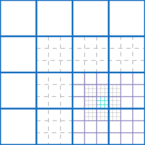
  Figure 2: Sketch of the mesh refinement structure of three AMR levels with refinement factor $\mathfrak{r}=3$. Solid lines indicate active cells, whereas the dashed ones are the virtual cells allowing interpolation between the coarse and the refined mesh, needed in the case of high order WENO reconstruction.

• A moving polygonal grid as the one described in [90] that i) moves with the fluid flow in order to reduce the numerical dissipation associated with transport terms and ii) also allows for topology changes at any time step in order to maintain always a high quality of the moving mesh; in this case we remark that our method is also able to deal with degenerate space time control volumes at arbitrary high order of accuracy.

2.2.1 Space-time connectivity

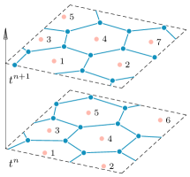
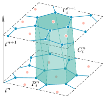
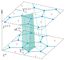
Figure 3: Space time connectivity. Left: The tessellation at time $t^{n}$ and time $t^{n+1}$. Middle: $P_{i}^{n}$ is connected with $P_{i}^{n+1}$ to construct the space–time control volume $C_{i}^{n}$. Right: The sub-triangle $T_{i_{j}}^{n}$ is connected with $T_{i_{j}}^{n+1}$ to construct the sub–space–time control volume $sC_{i_{j}}^{n}$.

To better understand the context of moving meshes we refer the reader to Figure 3: note that the tessellation at time $t^{n}$ has been evolved resulting in a slightly different tessellation at time $t^{n+1}$; for each element $P_{i}^{n}$ the new vertex coordinates $\mathbf{x}_{k}^{n+1}$, $k=1,\dots,N_{V_{i}}^{n}$, are connected to the old coordinates $\mathbf{x}_{k}^{n+1}$ via straight line segments, yielding the multidimensional space-time control volume $C_{i}^{n}$, that involves $N_{V_{i}}^{n,st}+2$ space-time sub-surfaces. Specifically, the space-time volume $C_{i}^{n}$ is bounded on the bottom and on the top by the element configuration at the current time level $P^{n}_{i}$ and at the new time level $P^{n+1}_{i}$, respectively, while it is closed with a total number of $N_{V_{i}}^{n,st}$ lateral space–time surfaces $\partial C_{i_{j}}^{n},j=1,\dots,N_{V_{i}}^{n,st}$ that are given by the evolution of each edge $e_{i_{j}}^{n}$ of element $P_{i}^{n}$ within the time step $\Delta t=t^{n+1}-t^{n}$. A priori, $\partial C_{i_{j}}^{n}$ are not parallel to the time direction: thus to be treated numerically they can be mapped to a reference square by using a set of of bilinear basis functions (see [21]). To resume, the space-time volume $C_{i}^{n}$ is bounded by its surface $\partial C^{n}_{i}$ which is given by

$$\partial C^{n}_{i}=\left(\bigcup\limits_{j}\partial C^{n}_{i_{j}}\right)\,\,\cup\,\,P_{i}^{n}\,\,\cup\,\,P_{i}^{n+1}.$$ (4)

Note that in the fixed Cartesian case, $C_{i}^{n}$ reduces to a right parallelepiped with four lateral space–time surfaces $\partial C_{i_{j}}^{n}$ parallel to the time-direction, so many simplifications are possible.

We close this part by emphasizing that the family of direct ALE schemes proposed in this work, based on the ADER predictor-corrector approach, is based on the integration of the governing equation (1) in space and in time directly over these space–time control volumes, see Section 2.7. Note that this procedure, which is more evident when $C_{i}^{n}$ is an oblique prism, is also hidden when $C_{i}^{n}$ is just a right parallelepiped.

2.3 Data representation

The conserved variables $\mathbf{Q}$ in (1) are discretized in each polygon $P_{i}^{n}$ at the current time $t^{n}$ via piecewise polynomials of arbitrary high order $N$, denoted by $\mathbf{u}_{h}^{n}(\mathbf{x},t^{n})$ and defined as

$$\mathbf{u}_{h}^{n}(\mathbf{x},t^{n})=\sum\limits_{\ell=0}^{\mathcal{N}-1}\varphi_{\ell}(\mathbf{x},t^{n})\,\hat{\mathbf{u}}^{n}_{\ell,i}=\varphi_{\ell}(\mathbf{x},t^{n})\,\hat{\mathbf{u}}^{n}_{\ell,i},\quad\mathbf{x}\in P_{i}^{n},$$ (5)

where in the last equality we have employed the classical tensor index notation based on the Einstein summation convention, which implies summation over two equal indices. The functions $\varphi_{\ell}(\mathbf{x},t^{n})$ can be either:

• Nodal spatial basis functions given by a set of Lagrange interpolation polynomials of maximum degree $N$ with the property

  $$\varphi_{\ell}(\mathbf{x}_{\text{GL}}^{m})=\left\{\begin{array}[]{rl}1&\text{if}\;\;\ell=m;\\ 0&\text{otherwise};\end{array}\right.\hskip 19.91684pt\ell,m=1,\ldots,(N+1)^{\text{d}},$$ (6)

  where $\{\mathbf{x}_{\text{GL}}^{m}\}$ are the set of the Gauss-Legendre (GL) quadrature points on $P_{i}^{n}$ (see [169] for the multidimensional case).

  In particular, when employing these basis functions on a Cartesian grid, each quadrilateral $P_{i}^{n}$ is easily mapped to a reference square, we only need the tensor product of the GL quadrature points in the unit interval $[0,1]$, and the $\varphi_{\ell}$ are simply generated by multiplying one-dimensional nodal basis functions, i.e

  $$\varphi_{\ell}(\mathbf{x},t^{n})=\varphi_{\ell_{1}}\left(\xi(x)\right)\varphi_{\ell_{2}}\left(\eta(y)\right)$$ (7)

  with $\varphi_{\ell_{i}}$ satisfying (6) with $d=1$, and $x=x_{j-\frac{1}{2}}+\xi\Delta x_{j}$, $y=y_{k-\frac{1}{2}}+\eta\Delta y_{k}$ being the set of reference coordinates related to $P_{i}^{n}$. In this case, the total number of GL quadrature points per polygon, as well as the total number of basis functions $\{\varphi_{\ell}\}$ and expansion coefficients $\hat{\mathbf{u}}^{n}_{\ell,i}$, the so-called degrees of freedom (DOF), is $\mathcal{N}=(N+1)^{d}$. These basis functions are used on Cartesian grids, i.e. for Case A.

• Modal spatial basis functions written through a Taylor series of degree $N$ in the variables $\mathbf{x}=(x,y)$ directly defined on the physical element $P_{i}^{n}$, expanded about its current barycenter $\mathbf{x}_{\mathbf{b}_{i}}^{n}$ and normalized by its current characteristic length $h_{i}$

  $$\varphi_{\ell}(\mathbf{x},t^{n})|_{P_{i}^{n}}=\frac{(x-{x}_{{b}_{i}}^{n})^{p_{\ell}}}{p_{\ell}!\,h_{i}^{p_{\ell}}}\,\frac{(y-{y}_{{b}_{i}}^{n})^{q_{\ell}}}{q_{\ell}!\,h_{i}^{q_{\ell}}},\qquad\ell=0,\dots,\mathcal{N}-1,\quad\ 0\leq p_{\ell}+q_{\ell}\leq N,$$ (8)

  $h_{i}$ being the radius of the circumcircle of $P_{i}^{n}$. In this case the total number $\mathcal{N}$ of DOF $\hat{\mathbf{u}}^{n}_{l}$ is $\mathcal{N}=\frac{1}{d!}\prod\limits_{m=1}^{d}(N+m).$ We employ this kind of basis functions in the moving unstructured polygonal Case B.

The discontinuous finite element data representation (5) leads naturally to discontinuous Galerkin (DG) schemes if $N>0$, but also to finite volume (FV) schemes in the case $N=0$. This indeed means that for $N=0$ we have $\varphi_{\ell}(\mathbf{x})=1$, with $\ell=0$ and (5) reduces to the classical piecewise constant data that are typical of finite volume methods. In the case $N>0$ (DG) the form given by (5) already provides a spatially high order accurate data representation with accuracy $N+1$, where instead for the case $N=0$ (FV), if we are interested in increasing the spatial order of accuracy, up to $M+1$ for examle, we need to perform a spatial reconstruction. With this notation, our method falls within the more general class of $P_{N}P_{M}$ schemes introduced in [61] for fixed unstructured meshes.

2.4 Data reconstruction

In this section we focus on the reconstruction procedure needed in the finite volume context ($N=0$, $M>0$) in order to obtain order of accuracy $M+1$ in space starting from the piecewise constant values of $\mathbf{u}_{h}^{n}(\mathbf{x},t^{n})$ in $P_{i}^{n}$ and its neighbors, i.e. in order to obtain a high order polynomial of degree $M$ representing our solution in each $P_{i}^{n}$

$$\mathbf{w}_{h}^{n}(\mathbf{x},t^{n})=\sum\limits_{\ell=0}^{\mathcal{M}-1}\psi_{\ell}(\mathbf{x},t^{n})\,\hat{\mathbf{w}}^{n}_{\ell,i}=\psi_{\ell}(\mathbf{x},t^{n})\,\hat{\mathbf{w}}^{n}_{\ell,i},\mathbf{x}\in P_{i}^{n},$$ (9)

where the $\psi_{\ell}$ functions simply coincide with the $\varphi_{\ell}$ basis functions of (5). Our reconstruction procedures are based on the WENO algorithm in its polynomial formulation as presented in [64, 71, 70, 175, 185, 132, 62, 164], and not based on the original version of WENO proposed in [120, 7, 114, 194] which provides only point values. For each $P_{i}^{n}$, the basic idea consists in i) selecting a central stencil of elements $\mathcal{S}_{i}^{0}$ with a total number of

$$n_{e}=f\cdot\frac{1}{d!}\prod\limits_{m=1}^{d}(M+m)$$ (10)

elements, containing the cell $P_{i}^{n}$ itself, its first layer of Voronoi neighbors $\mathcal{V}(P_{i}^{n})$ and filled by recursively adding neighbors of those elements that have been already included in the stencil, and in ii) using the cell-average values of the elements of $\mathcal{S}_{i}^{0}$ to reconstruct a polynomial of degree $M$ by imposing the integral conservation criterion, i.e by requiring that its average on each cell match the known cell average. If $f>1$ (which occurs in the unstructured case, where we take $f=1.5$), this of course leads to an overdetermined linear system, which is solved using a constrained least-squares technique (CLSQ) [70], i.e. the reconstructed polynomial has exactly the cell average $\hat{\mathbf{u}}^{n}_{0,i}$ on the polygon $P_{i}^{n}$ and matches all the other cell averages of the remaining stencil elements in the least-square sense.

However, as well known thanks to the Godunov theorem ([101]), the use of only one central stencil (which is indeed a linear procedure) would introduce oscillations in the presence of shock waves or other discontinuities. So, in order to make the reconstruction procedure nonlinear, we will compute the final reconstruction polynomial as a nonlinear combination or more than only one reconstruction polynomial, each one defined on a different reconstruction stencil $\mathcal{S}_{i}^{s}$.

We refer to the cited literature for further details, and here we just highlight the main characteristics of the two reconstruction procedures adopted in this work.

Case A: Cartesian mesh.

In Case A, of a fixed Cartesian mesh, we employ the polynomial WENO procedure given in [80], which is implemented in a dimension by dimension fashion. For each cell, we define its related sets of one-dimensional reconstruction stencils as

$$\mathcal{S}^{s,x}_{i}=\displaystyle{\bigcup_{m=j-L}^{j+R}}P_{mk}^{n},\quad\mathcal{S}^{s,y}_{i}=\displaystyle{\bigcup_{m=k-L}^{k+R}}P_{jm}^{n},$$ (11)

where $L=\{M,s\}$ and $R=\{M,s\}$ denote the order and stencil dependent spatial extension of the stencil to the left and to the right. For odd order schemes we consider three stencils, one central, one fully left–sided, and one fully right–sided stencil in each space dimension (see Figure 4 for a graphical interpretation for $M=2$), while for even order schemes we have four stencils, two of which are central, while the remaining two are again given by the fully left–sided and fully right–sided in each space dimension. In both cases the total amount of elements in each stencil is always $n_{e}=M+1$, the order of the scheme.

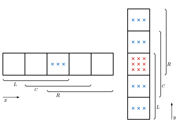
Figure 4: Reconstruction stencils for a fixed Cartesian mesh with $M=2$, where $L$, $C$ and $R$ denote the left–sided, central and right–sided stencils, respectively. Left: reconstruction on $x$ direction. Right: reconstruction on $y$ direction.

Focusing on the reconstruction procedure on the $x$ direction, given a element $P_{i}^{n}$, we start by expressing the first coordinate of the reconstruction polynomial at each stencil in terms of one dimensional basis functions,

$$\mathbf{w}^{s,x}_{h}(x,t^{n})=\sum_{\ell_{1}=0}^{M}\psi_{\ell_{1}}\left(\xi\right)\hat{\mathbf{w}}^{n,s}_{jk,\ell_{1}}=\psi_{\ell_{1}}\left(\xi\right)\hat{\mathbf{w}}^{n,s}_{jk,\ell_{1}}.$$ (12)

Then, we integrate on the stencil elements obtaining an algebraic system on the polynomial coefficients:

$$\frac{1}{\Delta x_{m}}\int_{x_{m-\frac{1}{2}}}^{x_{m+\frac{1}{2}}}\psi_{\ell_{1}}\left(\xi(x)\right)\hat{\mathbf{w}}^{n,s}_{jk,\ell_{1}}dx=\bar{\mathbf{u}}^{n}_{mk},\quad\forall P_{mk}^{n}\in\mathcal{S}^{s,x}_{i}$$ (13)

with $\bar{\mathbf{u}}^{n}_{mk}$ the average value obtained by integrating the solution at the previous time step on the cell $P_{mk}$. Once the coefficients, and thus the polynomials, related to all the stencils are obtained, we compute a reconstruction polynomial in the $x$ direction as the data-dependent nonlinear combination of these,

$$\mathbf{w}^{x}_{h}\left(x,t^{n}\right)=\psi_{\ell_{1}}\left(\xi\right)\hat{\mathbf{w}}^{n}_{jk,\ell_{1}},\quad\hat{\mathbf{w}}^{n}_{jk,\ell_{1}}=\sum_{s=1}^{n_{s}}\omega_{s}\hat{\mathbf{w}}^{n,s}_{jk,\ell_{1}},$$ (14)

where $n_{s}$ is the number of stencils, $n_{s}=3$ if $M=\dot{2}$ and $n_{s}=4$ otherwise; and $\omega_{s}$ denote the nonlinear weights (see [80] for further details).

To complete the reconstruction polynomial, we now repeat the above procedure in the $y$ direction for each degree of freedom $\hat{\mathbf{w}}^{n}_{jk,\ell_{1}}$. First, we write the reconstruction polynomial in terms of the basis functions,

$$\mathbf{w}^{s,y}_{h}(x,y,t^{n})=\psi_{\ell_{1}}\left(\xi\right)\psi_{\ell_{2}}\left(\eta\right)\hat{\mathbf{w}}^{n,s}_{jk,\ell_{1}\ell_{2}}.$$ (15)

Then, we solve the algebraic system

$$\frac{1}{\Delta y_{m}}\int_{y_{m-\frac{1}{2}}}^{y_{m+\frac{1}{2}}}\psi_{\ell_{2}}\left(\eta\left(y\right)\right)\hat{\mathbf{w}}^{n,s}_{jk,\ell_{1}\ell_{2}}dy=\hat{\mathbf{w}}^{n}_{jm,\ell_{1}},\quad\forall P_{jm}^{n}\in\mathcal{S}^{s,y}_{i}$$ (16)

and calculate

$$\hat{\mathbf{w}}^{n}_{jk,\ell_{1}\ell_{2}}=\sum_{s=1}^{n_{s}}\omega_{s}\hat{\mathbf{w}}^{n,s}_{jk,\ell_{1}\ell_{2}}.$$ (17)

Finally, we get the WENO reconstruction polynomial

$$\mathbf{w}_{h}^{n}\left(\mathbf{x},t^{n}\right)=\psi_{\ell_{1}}\left(\xi\right)\psi_{\ell_{2}}\left(\eta\right)\hat{\mathbf{w}}^{n}_{jk,\ell_{1}\ell_{2}}.$$ (18)

In order to enforce bounds on the WENO reconstruction polynomial, such as the condition $0\leq\alpha\leq 1$ on the volume fraction function of for example (56a), we rescale the reconstruction coefficients $\hat{\mathbf{w}}^{n}_{jk,\ell_{1}\ell_{2}}$ around the cell average as follows:

$$\hat{\mathbf{w}}^{*}_{jk,\ell_{1}\ell_{2}}=\bar{\mathbf{u}}^{*}_{jk}+\varphi_{jk}\left(\hat{\mathbf{w}}^{n}_{jk,\ell_{1}\ell_{2}}-\bar{\mathbf{u}}^{*}_{jk}\right),$$ (19)

where the scaling factor $\varphi_{jk}$ is computed via the Barth and Jespersen limiter (see [9]) applied to the volume fraction function $\alpha$ in all Gauss-Legendre and Gauss-Lobatto quadrature nodes, i.e. $\varphi_{jk}=\min(\varphi_{jk,p})$ is the global minimum in each element, with the nodal limiter values given by

$$\varphi_{jk,p}=\left\{\begin{array}[]{ccc}\min\left(1,\frac{\alpha_{\max}-\bar{\alpha}}{\alpha_{p}-\bar{\alpha}}\right),&\textnormal{ if }&\alpha_{p}-\bar{\alpha}>0,\\ \min\left(1,\frac{\alpha_{\min}-\bar{\alpha}}{\alpha_{p}-\bar{\alpha}}\right),&\textnormal{ if }&\alpha_{p}-\bar{\alpha}>0,\\ 1,&\textnormal{ if }&\alpha_{p}-\bar{\alpha}=0.\end{array}\right.$$ (20)

Here $\alpha_{\max}=1-\varepsilon\leq 1$ is the upper bound of the volume fraction function and $\alpha_{\min}=\varepsilon\geq 0$ is its lower bound; $\bar{\alpha}$ denotes the cell average of $\alpha$ and $\alpha_{p}$ denotes the node value of $\alpha$ in the quadrature point $\mathbf{x}_{p}$ under consideration. As already mentioned above, this strategy is inspired from the Barth and Jespersen limiter [9], but also from the new bound-preserving polynomial approximation introduced in [54, 39]. Since the physical solution of $\alpha$ must satisfy $0\leq\alpha\leq 1$, the above bound preserving limiter does not reduce the formal order of accuracy of the reconstruction, as proven in [54].

Case B: moving polygonal mesh.

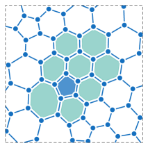
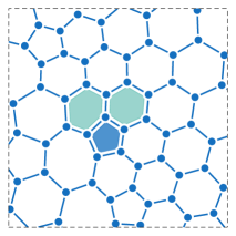
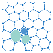
Figure 5: Stencils for the CWENO reconstruction of order three ($M=2$) with $f=1.5$ for a pentagonal element $P_{i}^{n}$. Left: central stencil made of the element itself $P_{i}^{n}$ (in violet) and $n_{e}-1=8$ of its neighbors (in blue). In the other panels we report two of the $N_{V_{i}}^{n}=5$ sectorial stencils containing the element itself and two consecutive neighbors belonging to $\mathcal{V}(P_{i}^{n})$.

In Case B of our moving and topology changing polygonal mesh we adopt a CWENO reconstruction algorithm, first introduced in [130, 131, 133, 164], and which can be cast in the general framework described in [49]. We closely follow the work outlined in [62, 32] for unstructured triangular and tetrahedral meshes, and extended it to moving polygonal grids in [90].

We emphasize that the main advantages of such a procedure is that only one stencil (the central one) is required to contain the total amount of elements stated in (10) and only this one is used to construct a polynomial of degree $M$; the other ones are used to compute polynomials of lower degree. In particular, we consider $N_{V_{i}}^{n}$ stencils $S_{i}^{s}$, each of them containing exactly $\hat{n}_{e}=(d+1)$ cells, i.e. the central cell $P^{n}_{i}$ and two consecutive neighbors belonging to $\mathcal{V}(P_{i}^{n})$. Refer to Figure 5 for a graphical description of the stencils. For each stencil $S_{i}^{s}$ we compute a linear polynomial by solving a simple reconstruction system which is not overdetermined. According to the above mentioned literature, the reconstructed polynomial obtained via a nonlinear combination of the polynomial of degree $M$, computed over $S_{0}^{s}$, and of the $N_{V_{i}}^{n}$ linear polynomials, computed over $S_{i}^{s}$, maintains the order of convergence of the method and avoids unwanted spurious oscillations. In particular, in the case of moving meshes with topology changes, where the set of neighbors may change at any time step, the use of smaller so-called sectorial stencils significantly speeds up computations.

For the sake of uniform notation, in the DG case, i.e. when $N>0$ and $M=N$, we trivially impose that the reconstruction polynomial is given by the DG polynomial, i.e. $\mathbf{w}_{h}^{n}(\mathbf{x},t^{n})=\mathbf{u}_{h}^{n}(\mathbf{x},t^{n})$, which automatically implies that in the case $N=M$ the reconstruction operator is simply the identity.

2.5 Space-time predictor step

In this section we focus on the key feature, the element-local space-time predictor step, of our ADER FV-DG schemes: this part of the algorithm (the predictor) produces a high order approximation in both space and time of $\mathbf{Q}$ in all $P_{i}^{n}$. This allows to obtain a fully discrete one-step scheme that is uniformly high order accurate in both space and time.

The predictor step consists in a completely local procedure which solves the governing PDE (1) in the small, see [110], inside each space-time element $C_{i}^{n}$, and it only considers the geometry of volume $C_{i}^{n}$, the initial data $\mathbf{w}_{h}^{n}$ on $P_{i}^{n}$ and the governing equations (1), without taking into account any interaction between $C_{i}^{n}$ and its neighbors. Because of this absence of communications, we refer to it as local. The procedure finally provides, for each $C_{i}^{n}$, a space-time polynomial data representation $\mathbf{q}_{h}^{n}$, which serves as a predictor solution, only valid inside $C_{i}^{n}$, to be used for evaluating the numerical fluxes, the non-conservative products and the algebraic source terms when integrating the PDE in the final corrector step (see Section 2.7) of the ADER scheme.

The predictor $\mathbf{q}_{h}^{n}$ is a polynomial of degree $M$, which takes the following form

$$\mathbf{q}_{h}^{n}(\mathbf{x},t)=\sum_{\ell=0}^{\mathcal{Q}-1}\theta_{\ell}(\mathbf{x},t)\hat{\mathbf{q}}_{\ell}^{n},\qquad(\mathbf{x},t)\in C_{i}^{n},$$ (21)

where $\theta_{\ell}(\mathbf{x},t)$ can be either

• For fixed and adaptive Cartesian grids (Case A), nodal space-time basis functions of degree $M$ given by the product of one-dimensional nodal basis functions verifying (6) (with $d=1$),

  $$\theta_{\ell}(x,y,t)=\varphi_{\ell_{1}}\left(\xi(x)\right)\varphi_{\ell_{2}}\left(\eta(y)\right)\varphi_{\ell_{3}}\left(\tau(t)\right),$$ (22)

  two of them mapped to the unit interval $[0,1]$ as in (7) and with the time coordinate mapped to the reference time $\tau\in[0,1]$ via $t=t^{n}+\tau\Delta t$. In this case, the total number of GL quadrature points per cell, as well as the total number of DOF is $\mathcal{Q}=(M+1)^{d+1}$, see also Figure 6.

  

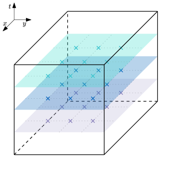
  Figure 6: Quadrature points on a space-time element, $C_{i}^{n}$, of a fixed Cartesian mesh with $M=2$.

• For our moving polygonal meshes (Case B), modal space time basis functions of degree $M$ in $d+1$ dimensions ($d$ space dimensions plus time) are used, which read

  $$\theta_{\ell}(x,y,t)|_{C_{i}^{n}}=\frac{(x-{x}_{{b}_{i}}^{n})^{p_{\ell}}}{{p_{\ell}}!\,h_{i}^{p_{\ell}}}\,\frac{(y-{y}_{{b}_{i}}^{n})^{q_{\ell}}}{{q_{\ell}}!\,h_{i}^{q_{\ell}}}\,\frac{(t-t^{n})^{q_{\ell}}}{{q_{\ell}}!\,h_{i}^{q_{\ell}}},\qquad\ell=0,\dots,\mathcal{Q},\quad 0\leq p_{\ell}+q_{\ell}+r_{\ell}\leq M,\\$$ (23)

  with the total number of DOF $\ \mathcal{Q}=\frac{1}{(d+1)!}\prod\limits_{m=1}^{d+1}(M+m)$, see also Figure 7.

  

  

  

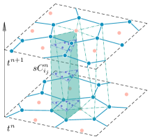
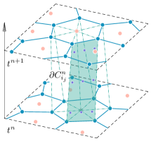
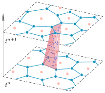
  Figure 7: Space–time quadrature points for third order methods, i.e. $M=2$, on a moving polygonal mesh with topology changes. Left: quadrature points for the volume integrals and the space–time predictor. Middle: quadrature points for the surface integrals, i.e. for flux computation. Right: quadrature points for the volume integrals and the space–time predictor of a sliver element.

Now, multiplying our PDE system (1) with a test function $\theta_{k}$ and integrating over the space-time control volume $C_{i}^{n}$ (see Section 2.2.1), we obtain the following weak form of the governing PDE, where both the test and the basis functions are time dependent

$$\int_{C_{i}^{n}}\theta_{k}(\mathbf{x},t)\frac{\partial\mathbf{q}_{h}^{n}}{\partial t}\,d\mathbf{x}\,dt+\int_{C_{i}^{n}}\theta_{k}(\mathbf{x},t)\left(\nabla\cdot\mathbf{F}(\mathbf{q}_{h}^{n})+\mathbf{B}(\mathbf{q}_{h}^{n})\cdot\nabla\mathbf{q}_{h}^{n}\right)\,d\mathbf{x}\,dt=\int_{C_{i}^{n}}\theta_{k}(\mathbf{x},t)\mathbf{S}(\mathbf{q}_{h}^{n})\,d\mathbf{x}\,dt\,.$$ (24)

Since we are only interested in an element local predictor solution, i.e. we do not need to consider the interactions with the neighbors, we do not yet take into account the jumps of $\mathbf{q}_{h}^{n}$ across the space–time lateral surfaces, because this will be done in the final corrector step (Section 2.7).

Instead, we insert the known discrete solution $\mathbf{w}_{h}^{n}(\mathbf{x},t^{n})$ at time $t^{n}$ in order to introduce a weak initial condition for solving our PDE; note that $\mathbf{w}_{h}^{n}(\mathbf{x},t^{n})$ uses information coming from the past only (following an upwinding approach) in such a way that the causality principle is correctly respected. To this purpose, the first term is integrated by parts in time. This leads to

$$\int_{P_{i}^{n+1}} \theta_{k}(\mathbf{x},t^{n+1})\mathbf{q}_{h}^{n}(\mathbf{x},t^{n+1})\,d\mathbf{x}-\int_{P_{i}^{n}}\theta_{k}(\mathbf{x},t^{n})\mathbf{w}_{h}^{n}(\mathbf{x},t^{n})\,d\mathbf{x}-\int_{C_{i}^{n}}\frac{\partial}{\partial t}\theta_{k}(\mathbf{x},t)\mathbf{q}_{h}^{n}(\mathbf{x},t)\,d\mathbf{x}\,dt$$ (25)

$$+\ \int_{C_{i}^{n}\backslash\partial C_{i}^{n}}\theta_{k}(\mathbf{x},t)\nabla\cdot\mathbf{F}(\mathbf{q}_{h}^{n})\,d\mathbf{x}\,dt=\int_{C_{i}^{n}\backslash\partial C_{i}^{n}}\theta_{k}(\mathbf{x},t)\left(\mathbf{S}(\mathbf{q}_{h}^{n})-\mathbf{B}(\mathbf{q}_{h}^{n})\cdot\nabla\mathbf{q}_{h}^{n}\right)\,d\mathbf{x}\,dt.$$

Equation (25) results in an element-local nonlinear system for the unknown degrees of freedom $\hat{\mathbf{q}}_{\ell}^{n}$ of the space-time polynomials $\mathbf{q}_{h}^{n}$. The solution of (25) can be found via a simple and fast converging fixed point iteration (a discrete Picard iteration) as detailed e.g. in [61, 112]. For linear homogeneous systems, the discrete Picard iteration converges in a finite number of at most $N+1$ steps, since the involved iteration matrix is nilpotent, see [117]. Moreover a proof of the convergence of this procedure in the case of a nonlinear homogeneous conservation law in 1D is given in next Section 2.6.

Simplification in the case of a fixed Cartesian mesh

The space-time predictor step formerly presented can be simplified in the case of a Cartesian mesh with nodal basis functions resulting in a more efficient algorithm. Under these assumptions the governing PDE (1), can be rewritten as

$$\frac{\partial\mathbf{Q}}{\partial\tau}+\frac{\partial\mathbf{f}^{\star}}{\partial\xi}+\frac{\partial\mathbf{g}^{\star}}{\partial\eta}+\mathbf{B}_{1}^{\star}\frac{\partial\mathbf{Q}}{\partial\xi}+\mathbf{B}_{2}^{\star}\frac{\partial\mathbf{Q}}{\partial\eta}=\mathbf{S}^{\star}$$ (26)

with

$$\mathbf{f}^{\star}=\frac{\Delta t}{\Delta x_{j}}\mathbf{f},\quad\mathbf{g}^{\star}=\frac{\Delta t}{\Delta y_{k}}\mathbf{g},\quad\mathbf{B}_{1}^{\star}=\frac{\Delta t}{\Delta x_{j}}\mathbf{B}_{1},\quad\mathbf{B}^{\star}_{2}=\frac{\Delta t}{\Delta y_{k}}\mathbf{B}_{2},\quad\mathbf{B}=\left[\mathbf{B}_{1},\mathbf{B}_{2}\right],\quad\mathbf{S}^{\star}=\Delta t\mathbf{S}.$$ (27)

Next, we multiply each term by a test function $\theta_{k}$ and we integrate over the reference space-time control volume $\mathcal{I}_{0}=\left[0,1\right]^{3}$

$$\int_{0}^{1}\int_{0}^{1}\int_{0}^{1} \theta_{k}\left(\frac{\partial\mathbf{Q}}{\partial\tau}+\frac{\partial\mathbf{f}^{\star}\left(\mathbf{Q}\right)}{\partial\xi}+\frac{\partial\mathbf{g}^{\star}\left(\mathbf{Q}\right)}{\partial\eta}\right)d\xi d\eta d\tau$$ (28)

$$=\int_{0}^{1}\int_{0}^{1}\int_{0}^{1}\theta_{k}\left(\mathbf{S}^{\star}\left(\mathbf{Q}\right)-\mathbf{B}_{1}^{\star}\left(\mathbf{Q}\right)\frac{\partial\mathbf{Q}}{\partial\xi}-\mathbf{B}_{2}^{\star}\left(\mathbf{Q}\right)\frac{\partial\mathbf{Q}}{\partial\eta}\right)d\xi d\eta d\tau.$$

Now, by substituting the discrete space-time predictor solution $\mathbf{q}_{h}^{n}$ with its expansion on the nodal basis and after integrating by parts in time, we obtain

$$\int_{0}^{1} \int_{0}^{1}\int_{0}^{1}\theta_{k}\left(\xi,\eta,1\right)\theta_{\ell}\left(\xi,\eta,1\right)\hat{\mathbf{q}}_{\ell}^{n}d\xi d\eta d\tau+\int_{0}^{1}\int_{0}^{1}\int_{0}^{1}\frac{\partial\theta_{k}\left(\xi,\eta,\tau\right)}{\partial\tau}\theta_{\ell}\left(\xi,\eta,\tau\right)\hat{\mathbf{q}}_{\ell}^{n}d\xi d\eta d\tau$$ (29)

$$=\int_{0}^{1}\int_{0}^{1}\int_{0}^{1}\theta_{k}\left(\xi,\eta,0\right)\mathbf{w}_{h}^{n}\left(\xi,\eta,t^{n}\right)d\xi d\eta d\tau-\int_{0}^{1}\int_{0}^{1}\int_{0}^{1}\theta_{k}\left(\frac{\partial\mathbf{f}^{\star}\left(\mathbf{q}_{h}^{n}\right)}{\partial\xi}+\frac{\partial\mathbf{g}^{\star}\left(\mathbf{q}_{h}^{n}\right)}{\partial\eta}\right)d\xi d\eta d\tau$$

$$+\int_{0}^{1}\int_{0}^{1}\times\int_{0}^{1}\theta_{k}\left(\mathbf{S}^{\star}\left(\mathbf{q}_{h}^{n}\right)-\mathbf{B}_{1}^{\star}\left(\mathbf{q}_{h}^{n}\right)\frac{\partial\mathbf{q}_{h}^{n}}{\partial\xi}-\mathbf{B}_{2}^{\star}\left(\mathbf{q}_{h}^{n}\right)\frac{\partial\mathbf{q}_{h}^{n}}{\partial\eta}\right)d\xi d\eta d\tau.$$

To recover the value of the unknown degrees of freedom $\hat{\mathbf{q}}_{\ell}^{n}$, it is sufficient to solve the above equation locally for each element. One important advantage of using the nodal Gauss-Legendre basis is that the terms in (29) can be evaluated in a dimension-by-dimension fashion.

Space-time predictor for sliver space–time elements

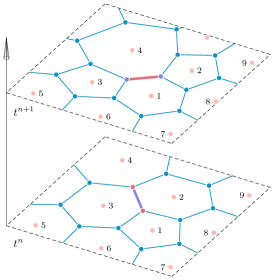
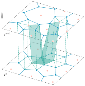
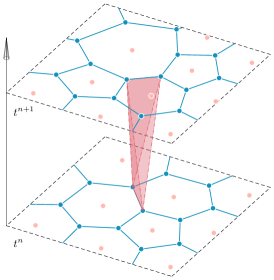
Figure 8: Space time connectivity with topology changes and sliver element. Left: at time $t^{n}$ the polygons $P_{2}^{n}$ and $P_{3}^{n}$ are neighbors and share the highlighted edge, instead at time $t^{n+1}$ they do not touch each other; the opposite situation occurs for polygons $P_{1}^{n}$ and $P_{4}^{n}$. This change of topology causes the appearance of degenerate elements of different types (refer to [90] for all the details). In particular, so-called space–time sliver elements (right) need to be taken into account when considering the space–time framework, so the predictor and the corrector step have to be a adapted to their special features. Sliver elements (right) are indeed completely new control volumes which do neither exist at time $t^{n}$, nor at time $t^{n+1}$, since they coincide with an edge of the tessellation and, as such, have zero areas in space. However, they have a non-negligible volume in space–time. The difficulties associated to this kind of element are due to the fact that $\mathbf{w}_{h}$ is not clearly defined for it at time $t^{n}$ (thus the predictor has to be modified) and that contributions across it should not be lost at time $t^{n+1}$ in order to guarantee conservation (thus the corrector has to be modified).

When a topology change occurs, some space–time sliver elements, as those shown on the right side of Figure 8, are originated (see [90]), and the predictor procedure over them needs particular care. The problem connected with sliver elements is the fact that their bottom face, which consists only in a line segment, is degenerate, hence the spatial integral over $P_{i}^{n}$ vanishes, i.e. there is no possibility to introduce an initial condition for the local Cauchy problem at time $t^{n}$ into their predictor. Thus, in order to couple however (24) with some known data from the past, we will end up with a formula different from (25). We underline that we first carry out the space–time predictor for all standard elements using, which can be computed independently of each other, and only subsequently we process the remaining space–time sliver elements. Then, when considering a sliver, we use the upwinding in time approach on the entire space–time surface $\partial C_{i}^{n}$ that closes a sliver control volume, and again respecting the causality principle, we take the information to feed the predictor only from the past, i.e. only from those space–time neighbors $C_{j}^{n}$ whose common surface $\partial C_{ij}^{n}$ exhibit a negative time component of the outward pointing space–time normal vector ($\tilde{\mathbf{n}}_{t}<0$). In this way, we can introduce information from the past into the space–time sliver elements.

As a consequence, the predictor solution $\mathbf{q}_{h}^{n}$ is again obtained by means of (24), but by treating the entire $\partial C_{i}^{n}$ with the upwind in time approach, i.e. by considering also the jump terms between the still unknown predictor of the slivers (call it $\mathbf{q}_{h}^{n,-}$) and the already known predictors of its neighbors (call them $\mathbf{q}_{h}^{n,+}$),

$$\int_{C_{i}^{n}}\theta_{k}(\mathbf{x},t)\frac{\partial}{\partial t}\mathbf{q}_{h}^{n}(\mathbf{x},t)\,d\mathbf{x}\,dt-\int_{\partial C_{i}^{-}}\theta_{k}(\mathbf{x},t^{n})\left((\mathbf{q}_{h}^{n,+}-\mathbf{q}_{h}^{n,-})-(\mathbf{B}\cdot\tilde{\mathbf{n}})(\mathbf{q}_{h}^{n,+}-\mathbf{q}_{h}^{n,-})\right)\,d\mathbf{S}\,dt$$ (30)

$$+\int_{C_{i}^{n}\backslash\partial C_{i}^{n}}\theta_{k}(\mathbf{x},t)\nabla\cdot\mathbf{F}(\mathbf{q}_{h}^{n})\,d\mathbf{x}\,dt=\int_{C_{i}^{n}\backslash\partial C_{i}^{n}}\theta_{k}(\mathbf{x},t)\left(\mathbf{S}(\mathbf{q}_{h}^{n})-\mathbf{B}(\mathbf{q}_{h}^{n})\cdot\nabla\mathbf{q}_{h}^{n}\right)\,d\mathbf{x}\,dt,$$

where $\partial C_{i}^{-}=\partial C_{i}^{n}\text{ with }\tilde{\mathbf{n}}_{t}<0$ is the part of the space-time boundary that has a negative time component of the space-time normal vector. Note that here we have taken into account also the jump of the nonconservative terms, and that these contributions have been added entirely (i.e. not only half of them, as in (49)). Indeed, in (49) half of the jump contribution goes to one element, while the other half goes to the neighboring element; here instead, since the interaction between neighbors is only computed from the side of the sliver element, the entire jump contributes to the predictor in the sliver element.

2.6 Convergence proof of the predictor step for a nonlinear conservation law

In this section, the convergence proof of the predictor for a nonlinear conservation law is given. The proof is provided, for simplicity, in the case of a fixed mesh in one space dimension, following the nomenclature already employed in Section 2.5, but it still holds in higher dimensions. Let us consider a general hyperbolic system of conservation laws of the form

$$\frac{\partial\mathbf{Q}}{\partial t}+\frac{\partial\mathbf{f}}{\partial x}=0.$$ (31)

Then, the corresponding space-time DG predictor used in the ADER-DG framework reads

$$\int\limits_{0}^{1}\int\limits_{0}^{1}\theta_{k}\frac{\partial\mathbf{q}_{h}}{\partial\tau}d\xi d\tau+\frac{\Delta t}{\Delta x}\,\int\limits_{0}^{1}\int\limits_{0}^{1}\theta_{k}\frac{\partial\mathbf{f}_{h}}{\partial\xi}d\xi d\tau=0.$$ (32)

For convenience, all derivatives and integrals in (32) have been transformed to the reference space-time element $[0,1]^{2}$. Moreover, the discrete solution is given by $\mathbf{q}_{h}=\theta_{l}(\xi,\tau)\hat{\mathbf{q}}_{\ell}$, and the flux is expanded in the same basis as $\mathbf{f}_{h}=\theta_{\ell}(\xi,\tau)\hat{\mathbf{f}}_{\ell}$. When using a nodal basis, we can compute the degrees of freedom for the flux interpolant $\mathbf{f}_{h}$ simply as $\hat{\mathbf{f}}_{\ell}=\mathbf{f}\left(\hat{\mathbf{q}}_{\ell}\right)$. We also recall that the initial condition given by the DG scheme at time $t^{n}$ reads $\mathbf{w}_{h}=\varphi_{\ell}(\xi)\hat{\mathbf{w}}_{\ell}$. Then, integration of the first term in (32) by parts in time yields

$$\int\limits_{0}^{1}\theta_{k}(\xi,1)\mathbf{q}_{h}d\xi-\int\limits_{0}^{1}\int\limits_{0}^{1}\frac{\partial\theta_{k}}{\partial\tau}\mathbf{q}_{h}d\xi d\tau+\frac{\Delta t}{\Delta x}\,\int\limits_{0}^{1}\int\limits_{0}^{1}\theta_{k}\frac{\partial\mathbf{f}_{h}}{\partial\xi}d\xi d\tau=\int\limits_{0}^{1}\theta_{k}(\xi,0)\mathbf{w}_{h}d\xi,$$ (33)

and insertion of the definitions of the discrete solution leads to

$$\left(\int\limits_{0}^{1}\theta_{k}(\xi,1)\theta_{l}(\xi,1)d\xi\,-\int\limits_{0}^{1}\int\limits_{0}^{1}\frac{\partial\mathbf{\theta}_{k}}{\partial\tau}\theta_{l}d\xi d\tau\,\right)\,\hat{\mathbf{q}}_{l}+\frac{\Delta t}{\Delta x}\,\int\limits_{0}^{1}\int\limits_{0}^{1}\theta_{k}\frac{\partial\mathbf{\theta}_{l}}{\partial\xi}d\xi d\tau\,\hat{\mathbf{f}}_{l}=\int\limits_{0}^{1}\theta_{k}(\xi,0)\varphi_{l}(\xi)d\xi\,\hat{\mathbf{w}}_{l}.$$ (34)

The iterative scheme employed to find the solution for the space-time degrees of freedom $\hat{\mathbf{q}}$, at any Picard iteration $r$, can therefore be rewritten in compact matrix-vector notation as

$$\mathbf{K}_{1}\hat{\mathbf{q}}^{r+1}+\frac{\Delta t}{\Delta x}\mathbf{K}_{\xi}\,\mathbf{f}\left(\hat{\mathbf{q}}^{r+1}\right)=\mathbf{F}_{0}\hat{\mathbf{w}}^{n}$$ (35)

with

$$\mathbf{K}_{1}=\int\limits_{0}^{1}\theta_{k}(\xi,1)\theta_{l}(\xi,1)d\xi\,-\int\limits_{0}^{1}\int\limits_{0}^{1}\frac{\partial\mathbf{\theta}_{k}}{\partial\tau}\theta_{l}d\xi d\tau,$$ (36)

$$\mathbf{K}_{\xi}=\int\limits_{0}^{1}\int\limits_{0}^{1}\theta_{k}\frac{\partial\mathbf{\theta}_{l}}{\partial\xi}d\xi d\tau,\qquad\mathbf{F}_{0}=\int\limits_{0}^{1}\theta_{k}(\xi,0)\varphi_{l}(\xi)d\xi,$$ (37)

where we have dropped the indices to ease the notation. After inverting $\mathbf{K}_{1}$ (this matrix is built using the linearly independent basis functions so that it is invertible), we obtain the explicit iteration formula

$$\hat{\mathbf{q}}^{r+1}=\mathbf{K}_{1}^{-1}\mathbf{F}_{0}\hat{\mathbf{w}}^{n}-\frac{\Delta t}{\Delta x}\mathbf{K}_{1}^{-1}\mathbf{K}_{\xi}\,\mathbf{f}\left(\hat{\mathbf{q}}^{r}\right).$$ (38)

To prove that the former iterative formula will converge, we introduce the operator

$$\bm{\varphi}\left(\hat{\mathbf{q}}\right)=\mathbf{K}_{1}^{-1}\mathbf{F}_{0}\hat{\mathbf{u}}^{n}-\frac{\Delta t}{\Delta x}\mathbf{K}_{1}^{-1}\mathbf{K}_{\xi}\,\mathbf{f}\left(\hat{\mathbf{q}}\right),$$ (39)

and the induced matrix norm

$$\left\|\mathbf{A}\right\|=\sup\limits_{\mathbf{x}\neq 0}\frac{\left\|\mathbf{A}\mathbf{x}\right\|}{\left\|\mathbf{x}\right\|}.$$ (40)

Furthermore, we assume the flux to be Lipschitz continuous with Lipschitz constant $L>0$ so that

$$\left\|\mathbf{f}\left(\hat{\mathbf{p}}\right)-\mathbf{f}\left(\hat{\mathbf{q}}\right)\right\|\leq L\left\|\hat{\mathbf{p}}-\hat{\mathbf{q}}\right\|.$$ (41)

We now need to show that the operator $\bm{\varphi}$ is a contraction:

$$\left\|\bm{\varphi}\left(\hat{\mathbf{q}}\right)-\bm{\varphi}\left(\hat{\mathbf{p}}\right)\right\| = \left\|\mathbf{K}_{1}^{-1}\mathbf{F}_{0}\hat{\mathbf{u}}^{n}-\mathbf{K}_{1}^{-1}\mathbf{F}_{0}\hat{\mathbf{u}}^{n}-\frac{\Delta t}{\Delta x}\mathbf{K}_{1}^{-1}\mathbf{K}_{\xi}\,\mathbf{f}\left(\hat{\mathbf{q}}\right)+\frac{\Delta t}{\Delta x}\mathbf{K}_{1}^{-1}\mathbf{K}_{\xi}\,\mathbf{f}\left(\hat{\mathbf{p}}\right)\right\|$$ (42)

$$= \frac{\Delta t}{\Delta x}\left\|\mathbf{K}_{1}^{-1}\mathbf{K}_{\xi}\,\left(\mathbf{f}\left(\hat{\mathbf{p}}\right)-\mathbf{f}\left(\hat{\mathbf{q}}\right)\right)\right\|$$

$$\leq \frac{\Delta t}{\Delta x}\left\|\mathbf{K}_{1}^{-1}\mathbf{K}_{\xi}\right\|\,\left\|\mathbf{f}\left(\hat{\mathbf{p}}\right)-\mathbf{f}\left(\hat{\mathbf{q}}\right)\right\|$$

$$\leq L\frac{\Delta t}{\Delta x}\left\|\mathbf{K}_{1}^{-1}\mathbf{K}_{\xi}\right\|\,\left\|\hat{\mathbf{p}}-\hat{\mathbf{q}}\right\|\,.$$

The operator is therefore a contraction under the CFL-type condition on the time step $\Delta t$

$$0<L\frac{\Delta t}{\Delta x}\left\|\mathbf{K}_{1}^{-1}\mathbf{K}_{\xi}\right\|<1,$$ (43)

which connects the Lipschitz constant $L$ with the mesh spacing $\Delta x$ and the matrix norm of $\left\|\mathbf{K}_{1}^{-1}\mathbf{K}_{\xi}\right\|$. Since the operator is contractive under the above assumptions, the Banach fixed point theorem, [8], guarantees convergence of the iterative method.

In the previous reasoning, we have assumed that the inequality in the right hand side of (43) be strict. Thus, to conclude the proof, let us assume that the equality holds, this is true if and only if $\left\|\mathbf{K}_{1}^{-1}\mathbf{K}_{\xi}\right\|=0$. By taking into account the definition of the induced matrix norm (40), it implies $\left\|\mathbf{K}_{1}^{-1}\mathbf{K}_{\xi}\,\mathbf{x}\right\|=0$ for any $\mathbf{x}$ in the metric space. Thus, $\mathbf{K}_{1}^{-1}\mathbf{K}_{\xi}=0$. Direct substitution in (38) gives

$$\mathbf{K}_{1}\hat{\mathbf{q}}^{r+1}=\mathbf{F}_{0}\hat{\mathbf{w}}^{n},$$ (44)

so that no iterative procedure is done.

Note: The matrix $\mathbf{K}_{1}^{-1}\mathbf{K}_{\xi}$ has been proven to be nilpotent and thus all its eigenvalues are zero, see [117], which guarantees convergence to the exact solution in a finite number of steps for linear homogeneous PDE.

2.7 Corrector step

The corrector step is the last step of our path-conservative ADER FV-DG scheme, where the update of the solution from time $t^{n}$ up to time $t^{n+1}$ can take place in a single step procedure thanks to the use of the predictor $\mathbf{q}_{h}^{n}$.

The update formula is recovered starting from the space–time divergence form of the PDE

$$\tilde{\nabla}\cdot\tilde{\mathbf{F}}(\mathbf{Q})+\tilde{\mathbf{B}}(\mathbf{Q})\cdot\tilde{\nabla}\mathbf{Q}=\mathbf{S}(\mathbf{Q}),\quad\tilde{\mathbf{F}}=(\mathbf{F},\mathbf{Q}),\quad\tilde{\mathbf{B}}=(\mathbf{B},\mathbf{0}),\ \text{ and }\ \tilde{\nabla}=\left(\partial_{\mathbf{x}},\,\partial_{t}\right)^{T},$$ (45)

which is multiplied by a set of space–time test functions $\tilde{\varphi}_{k}$ and integrated over each space–time control volume $C_{i}^{n}$

$$\int_{C_{i}^{n}}\tilde{\varphi}_{k}(\mathbf{x},t)\left(\nabla\cdot\tilde{\mathbf{F}}(\mathbf{Q})+\tilde{\mathbf{B}}(\mathbf{Q})\cdot\nabla\mathbf{Q}\right)\,d\mathbf{x}\,dt=\int_{C_{i}^{n}}\tilde{\varphi}_{k}(\mathbf{x},t)\mathbf{S}(\mathbf{Q})\,d\mathbf{x}\,dt\,.$$ (46)

Note that the employed test functions $\tilde{\varphi}_{k}$ coincide with the $\theta_{k}$ of (22) for the Cartesian Case A. Instead, for the moving polygonal Case B, they need to be tied to the motion of the barycenter $\mathbf{x}_{\mathbf{b}_{i}}(t)$ and must be moved together with $P_{i}(t)$ in such a way that at time $t=t^{n}$ they refer to the current barycenter $\mathbf{x}_{\mathbf{b}_{i}}^{n}$ and at time $t=t^{n+1}$ they refer to the new barycenter $\mathbf{x}_{\mathbf{b}_{i}}^{n+1}$, thus they are defined as follows

$$\tilde{\varphi}_{\ell}(x,y,t)|_{C_{i}^{n}}=\frac{(x-x_{b_{i}}(t))^{p_{\ell}}}{{p_{\ell}}!\,h_{i}^{p_{\ell}}}\,\frac{(y-y_{b_{i}}(t))^{q_{\ell}}}{{q_{\ell}}!\,h_{i}^{q_{\ell}}},\quad\text{ with }\ \mathbf{x}_{\mathbf{b}_{i}}(t)=\frac{t-t^{n}}{\Delta t}\mathbf{x}_{\mathbf{b}_{i}}^{n}+\left(1-\frac{t-t^{n}}{\Delta t}\right)\mathbf{x}_{\mathbf{b}_{i}}^{n+1},$$ (47)

$$\ell=0,\dots,\mathcal{N},\quad 0\leq p+q\leq N.$$

These moving modal basis functions are essential to the moving approach presented in [90] and used in this paper. They naturally allow for topology changes, without the need of any remapping steps, which we want to avoid in a direct ALE formulation.

Now, (46) by applying the Gauss theorem to the flux-divergence term and by splitting the non-conservative products into their volume and surface contribution, becomes

$$\int_{P_{i}^{n+1}}\tilde{\varphi}_{k}\mathbf{u}_{h}(\mathbf{x},t^{n+1})\,d\mathbf{x}=\int_{P_{i}^{n}}\tilde{\varphi}_{k}\mathbf{u}_{h}(\mathbf{x},t^{n})\,d\mathbf{x}-\sum_{j=1}^{N_{V_{i}}^{n,st}}\int_{\partial C_{ij}^{n}}\tilde{\varphi}_{k}\mathcal{D}(\mathbf{q}_{h}^{n,-},\mathbf{q}_{h}^{n,+})\cdot\mathbf{\tilde{n}}\,dS$$ (48)

$$+\int_{C_{i}^{n}\backslash\partial C_{i}^{n}}\tilde{\nabla}\tilde{\varphi}_{k}\cdot\tilde{\mathbf{F}}(\mathbf{q}_{h})\,d\mathbf{x}dt+\int_{C_{i}^{n}\backslash\partial C_{i}^{n}}\tilde{\varphi}_{k}(\mathbf{x},t)\left(\mathbf{S}(\mathbf{q}_{h}^{n})-\mathbf{B}(\mathbf{q}_{h}^{n})\cdot\nabla\mathbf{q}_{h}^{n}\right)\,d\mathbf{x}\,dt,$$

where $\mathbf{Q}$ on $P_{i}^{n+1}$ is represented by the unknown $\mathbf{u}_{h}^{n+1}$, on $P_{i}^{n}$ is taken to be the current representation of the conserved variables $\mathbf{u}_{h}^{n}$, in the interior of $C_{i}^{n}$ is given by the predictor $\mathbf{q}_{h}^{n}$ and on the space–time lateral surfaces $\partial C_{ij}^{n}$ is given by $\mathbf{q}_{h}^{n,-}$ and $\mathbf{q}_{h}^{n,+}$ which are the so-called boundary-extrapolated data, i.e. the values assumed respectively by the predictors of the two neighbor elements $C_{i}^{n}$ and $C_{j}^{n}$ on the shared space–time lateral surface $\partial C_{ij}^{n}$. Furthermore, we have employed a two-point path-conservative numerical flux function of Rusanov-type

$$\mathcal{D}(\mathbf{q}_{h}^{n,-},\mathbf{q}_{h}^{n,+})\cdot\mathbf{\tilde{n}}= \ \frac{1}{2}\left(\tilde{\mathbf{F}}(\mathbf{q}_{h}^{n,+})+\tilde{\mathbf{F}}(\mathbf{q}_{h}^{n,-})\right)\cdot\tilde{\mathbf{n}}-\frac{1}{2}s_{\max}\left(\mathbf{q}_{h}^{n,+}-\mathbf{q}_{h}^{n,-}\right)\,$$ (49)

$$+\frac{1}{2}\left(\int\limits_{0}^{1}\tilde{\mathbf{B}}\left(\mathbf{\Psi}(\mathbf{q}_{h}^{n,-},\mathbf{q}_{h}^{n,+},s)\right)\cdot\mathbf{n}\,d\mathbf{x}\right)\cdot\left(\mathbf{q}_{h}^{n,+}-\mathbf{q}_{h}^{n,-}\right),$$

where $s_{\max}$ is the maximum eigenvalue of the ALE Jacobian matrices $\mathbf{A}^{\!\!\mathbf{V}}_{\mathbf{n}}(\mathbf{q}_{h}^{n,+})$ and $\mathbf{A}^{\!\!\mathbf{V}}_{\mathbf{n}}(\mathbf{q}_{h}^{n,-})$ being

$$\mathbf{A}^{\!\!\mathbf{V}}_{\mathbf{n}}(\mathbf{Q})=\left(\sqrt{\tilde{n}_{x}^{2}+\tilde{n}_{y}^{2}}\right)\left[\frac{\partial\mathbf{F}}{\partial\mathbf{Q}}\cdot\mathbf{n}-(\mathbf{V}\cdot\mathbf{n})\,\mathbf{I}\right],\qquad\mathbf{n}=\frac{(\tilde{n}_{x},\tilde{n}_{y})^{T}}{\sqrt{\tilde{n}_{x}^{2}+\tilde{n}_{y}^{2}}},$$ (50)

and the path $\mathbf{\Psi}=\mathbf{\Psi}(\mathbf{q}_{h}^{-},\mathbf{q}_{h}^{+},s)$ is a straight-line segment path

$$\mathbf{\psi}=\mathbf{\psi}(\mathbf{q}_{h}^{-},\mathbf{q}_{h}^{+},s)=\mathbf{q}_{h}^{-}+s\left(\mathbf{q}_{h}^{+}-\mathbf{q}_{h}^{-}\right)\,,s\in[0,1]\,,$$ (51)

connecting $\mathbf{q}_{h}^{n,-}$ and $\mathbf{q}_{h}^{n,+}$ which allow to treat the jump of the non-conservative products following the theory introduced in [50, 146, 42], and extended to ADER FV-DG schemes of arbitrary high order in [63, 78]. Despite in this paper we only consider the Rusanov flux, the above methodology can be extended to different flux functions, adapting to the new flux splitting techniques like the ones presented in [181]. Finally, the time step size $\Delta t$ is given by

$$\Delta t<\text{CFL}\frac{h_{\text{min}}}{\left(2N+1\right)}\frac{1}{|\lambda_{\text{max}}|},\quad\text{(Case A)},\qquad\Delta t<\textnormal{CFL}\left(\!\!\frac{|P_{i}^{n}|}{(2N+1)\,|\lambda_{\max}|\,\sum_{\partial P_{i_{j}}^{n}}|\ell_{i_{j}}|}\!\!\right)\quad\text{(Case B)},$$ (52)

where $h_{\text{min}}$ is the minimum characteristic mesh-size, $\ell_{i_{j}}$ is the length of the edge $j$ of $P_{i}^{n}$ and $|\lambda_{\max}|$ is the spectral radius of the Jacobian of the flux $\mathbf{F}$. Stability on unstructured meshes is guaranteed by the satisfaction of the inequality $\textnormal{CFL}<\frac{1}{d}$, see [61].

We close this section by remarking that the integration of the governing PDE over closed space-time volumes $C_{i}^{n}$ automatically satisfies the geometric conservation law (GCL) for all test functions $\tilde{\varphi}_{k}$. This simply follows from the Gauss theorem and we refer to [22] for a complete proof.

2.8 A posteriori subcell finite volume limiter

Up to now, we have presented a family of FV and DG type schemes which achieves arbitrary high order of accuracy in space and time; the main difference between the FV and the DG approach lies in the fact that FV schemes, thanks to the WENO-type nonlinear reconstruction procedure, are robust in the presence of shocks and discontinuities, while the DG formulation as presented so far, being linear in the sense of Godunov, is subject to the appearance of spurious oscillations. Thus, in order to employ a DG scheme in the context of solving hyperbolic partial differential equations, where usually discontinuities are developed, a technique that is able to limit spurious oscillations (called limiter) should be introduced. Several attempts in that direction can be found in the literature. For example, we could recall the artificial viscosity technique used in [155, 147, 43] which consists in adding a small parabolic term in the equation in order to smooth out the discontinuities.

Here, instead, we follow a different approach based on exploiting the respective strengths of FV and DG schemes, i.e. the resolution of DG in smooth regions and the robustness of FV across discontinuities. Thus, we first evolve the solution everywhere by using our DG scheme; then, we check a posteriori, at the end of each time step, if the obtained DG solution in each cell respects or not some criteria (as density and pressure positivity, a relaxed discrete maximum principle, specific physical bounds, or more elaborate choices as those of [105]), and we mark as troubled those cells where the obtained DG solution is marked as not acceptable. Only for these troubled cells we repeat the time step using, instead of the DG scheme, a second order TVD FV method, which always assures a robust solution.

This idea is founded on works as those of [46, 153, 121, 4, 113, 134, 122, 123, 45, 55, 56, 135, 31, 30]; but in particular, here, we adopt a so-called subcell approach aimed at not losing the resolution of the DG scheme when switching to the FV method, as forwarded in [167, 81, 193, 73, 25, 83, 154, 52, 32]. Indeed, at the beginning of the time step we project the DG solution $\mathbf{u}_{h}^{n}$ of a troubled cell $P_{i}^{n}$ on a subdivision of it in sub-cells $s_{i,\alpha}^{n}$ obtaining a value for the cell averages on $s_{i,\alpha}^{n}$ at time $t^{n}$

$$\mathbf{v}_{i,\alpha}^{n}(\mathbf{x},t^{n})=\frac{1}{|s_{i,\alpha}^{n}|}\int_{s_{i,\alpha}^{n}}\mathbf{u}_{h}^{n}(\mathbf{x},t^{n})\,d\mathbf{x}=\frac{1}{|s_{i,\alpha}^{n}|}\int_{s_{i,\alpha}^{n}}\varphi_{\ell}(\mathbf{x})\,d\mathbf{x}\,\hat{\mathbf{u}}^{n}_{l}=\mathcal{P}(\mathbf{u}_{h}^{n})\qquad\forall\alpha.$$ (53)

We evolve the cell averages up to time $t^{n+1}$ using a classical TVD FV scheme, obtaining $\mathbf{v}_{i,\alpha}^{n+1}(\mathbf{x},t^{n+1})$. Finally, we recover a DG polynomial representation of the solution at time $t^{n+1}$ over $P_{i}^{n+1}$ using the values on the sub-grid level $\mathbf{v}_{i,\alpha}^{n+1}$ and by applying a reconstruction operator as

$$\int_{S_{i,\alpha}^{n}}\mathbf{u}_{h}^{n+1}(\mathbf{x},t^{n+1})\,d\mathbf{x}=\int_{S_{i,\alpha}^{n}}\mathbf{v}_{i,\alpha}^{n+1}(\mathbf{x},t^{n})\,d\mathbf{x}=\mathcal{R}(\mathbf{v}_{i,\alpha}^{n+1}(\mathbf{x},t^{n}))\qquad\forall\alpha,$$ (54)

where the reconstruction is imposed to be conservative on the main cell $P_{i}^{{n+1}}$ yielding the additional linear constraint

$$\int_{P_{i}^{{n+1}}}\mathbf{u}_{h}(\mathbf{x},t^{n+1})\,d\mathbf{x}=\int_{P_{i}^{{n+1}}}\mathbf{v}_{h}(\mathbf{x},t^{n+1})\,d\mathbf{x}.$$ (55)

Thus, the limited solution on a troubled cell is robust thanks to the use of a TVD scheme and accurate thanks to the subcell resolution.

For all the details of the a posteriori subcell FV limiter used in this work, we refer to [81, 82] for the fixed Cartesian Case A and to [90] for the moving polygonal Case B.

3 A unified first order hyperbolic model of continuum mechanics

3.1 Governing PDE system

A simplified diffuse interface formulation of the unified continuum fluid and solid mechanics model [150, 76, 77, 75], which can be used for modeling moving boundary problems of fluids and solids of arbitrary geometry, is given by the following PDE system (throughout this paper we make use of the Einstein summation convention over repeated indices)

$$\frac{\partial\alpha}{\partial t}+v_{k}\frac{\partial\alpha}{\partial x_{k}}=0,$$ (56a)

$$\frac{\partial(\alpha\rho)}{\partial t}+\frac{\partial(\alpha\rho v_{k})}{\partial x_{k}}=0,$$ (56b)

$$\frac{\partial(\alpha\rho v_{i})}{\partial t}+\frac{\partial\left(\alpha\rho v_{i}v_{k}+\alpha p\delta_{ik}-\alpha\sigma_{ik}\right)}{\partial x_{k}}=\rho g_{i},$$ (56c)

$$\frac{\partial A_{ik}}{\partial t}+\frac{\partial(A_{ij}v_{j})}{\partial x_{k}}+v_{j}\left(\frac{\partial A_{ik}}{\partial x_{j}}-\frac{\partial A_{ij}}{\partial x_{k}}\right)=-\frac{1}{\theta_{1}(\tau_{1})}E_{A_{ik}},$$ (56d)

$$\frac{\partial(\alpha\rho J_{i})}{\partial t}+\frac{\partial\left(\alpha\rho J_{i}v_{k}+T\delta_{ik}\right)}{\partial x_{k}}=-\frac{1}{\theta_{2}(\tau_{2})}E_{J_{i}},$$ (56e)

$$\frac{\partial(\alpha\rho S)}{\partial t}+\frac{\partial\left(\alpha\rho Sv_{k}+E_{J_{k}}\right)}{\partial x_{k}}=\frac{\rho}{T}\left(\frac{1}{\theta_{1}}E_{A_{ik}}E_{A_{ik}}+\frac{1}{\theta_{2}}E_{J_{k}}E_{J_{k}}\right)\geq 0,$$ (56f)

$$\frac{\partial(\alpha\rho{E})}{\partial t}+\frac{\partial\left(v_{k}\alpha\rho{E}+\alpha v_{i}(p\delta_{ik}-\sigma_{ik})\right)}{\partial x_{k}}=\rho g_{i}v_{i}.$$ (56g)

Here, (56a) is the evolution equation for the color function $\alpha$ that is needed in the diffuse interface approach as introduced in [173] for the description of linear elastic solids of arbitrary geometry and as used in [59, 91] for a simple diffuse interface method for the simulation of non-hydrostatic free surface flows. We assume that the color function $\alpha$ equals to 1 in the regions of the computational domain occupied by the material and 0 outside these regions. In the computational code, $\alpha=1-\varepsilon$ inside of the material and $\alpha=\varepsilon$ outside the material. Here, $\varepsilon$ is a small parameter $\varepsilon\ll 1$, see Section 4. Then, inside of the diffuse interface, $\alpha$ may take any values between 0 and 1 (between $\varepsilon$ and $1-\varepsilon$ in the computational code). Equation (56b) is the mass conservation law and $\rho$ is the material density; (56c) is the momentum conservation law, where $v_{i}$ is the velocity field and $g_{i}$ is the gravity vector; (56d) is the evolution equation for distortion field $A_{ik}$ (non-holonomic basis triad, see [151]); (56e) is the evolution equation for the specific thermal impulse $J_{k}$ constituting the heat conduction in the matter via a hyperbolic (non Fourier–type) model. Finally, (56f) is the entropy balance equation and (56g) is the energy conservation law. Other thermodynamic parameters are defined via the total energy potential $E=E(\alpha,\rho,S,{\bm{v}},{\bm{A}},{\bm{J}})$: $\Sigma_{ik}=p\delta_{ik}-\sigma_{ik}$ is the total stress tensor ($\delta_{ik}$ is the Kronecker delta); $p=\rho^{2}E_{\rho}$ is the thermodynamic pressure; $\sigma_{ik}=-\rho A_{jk}E_{A_{ji}}$ is the non-isotropic part of the stress tensor, $T=E_{S}$ is the temperature, and the notations such as $E_{\rho}$, $E_{A_{ik}}$, etc. stand for the partial derivatives of the energy potential, e.g. $E_{\rho}=\frac{\partial E}{\partial\rho}$, $E_{A_{ik}}=\frac{\partial E}{\partial A_{ik}}$, etc.

The dissipation in the medium includes two relaxation processes: the shear stress relaxation characterized by the scalar function $\theta_{1}(\tau_{1})>0$ depending on the relaxation time $\tau_{1}$ and thermal impulse relaxation characterized by $\theta_{2}(\tau_{2})>0$ depending on the relaxation time $\tau_{2}$. Both these relaxation processes then contribute to the entropy production term (the source on the right hand-side of (56f)) which is positive because it is quadratic in $E_{A_{ik}}$ and $E_{J_{k}}$.

From the mathematical standpoint, the unification of the model (56) consists in the use of only first-order hyperbolic equations for both dissipative and non-dissipative processes in contrast to the classical continuum mechanics relying on the mixed hyperbolic-parabolic formulations such as the famous Navier-Stokes-Fourier equations, for example. From the physical standpoint, the unification of equations (56) consists in treating solid and fluid states of matter from the solid-dynamics viewpoint. Indeed, as discussed in [150, 76, 75], similarly to standard continuum solid-dynamics, the distortion field introduces additional degrees of freedom (in comparison to the classical continuum fluid mechanics) which characterizes deformation and rotational degrees of freedom of the continuum particles, represented not as scaleless mathematical points but characterized by a finite length scale, or equivalently, time scale $\tau_{1}$, e.g. see [75]. In such a formulation, solid-type behavior corresponds to relaxation times $\tau_{1}$ such that $T^{problem}\ll\tau_{1}$, while the fluid-type behavior corresponds to $\tau_{1}\ll T^{problem}$, where $T^{problem}$ is the characteristic time scale of the problem under consideration.

In order to close system (56), that is, in order to define pressure $p=\rho^{2}E_{\rho}$, stresses $\sigma_{ik}=-\rho A_{jk}E_{A_{ji}}$, temperature $T=E_{S}$, and the dissipative source terms, one needs to provide the energy potential $E$. In this paper, we rely on a rather simple choice of $E$, which is, however, enough to deal with Newtonian fluids and simple hyperelastic solids. Thus, we assume that the specific total energy can be written as a sum of three contributions as

$$E(\alpha,\rho,S,v_{i},A_{ik},J_{k})=E_{1}(\rho,S)+E_{2}(\alpha,A_{ik},J_{k})+E_{3}(v_{i}),$$ (57)

with the specific internal energy given by the ideal gas equation of state

$$E_{1}(\rho,S)=\frac{c_{0}^{2}}{\gamma(\gamma-1)},\ c_{0}^{2}=\gamma\rho^{\gamma-1}e^{S/c_{v}},\quad\text{or}\quad E_{1}(\rho,p)=\frac{p}{\rho(\gamma-1)},$$ (58)

in the case of gases, and given by either the so-called stiffened gas equation of state

$$E_{1}(\rho,S)=\frac{c_{0}^{2}}{\gamma(\gamma-1)}\left(\frac{\rho}{\rho_{0}}\right)^{\gamma-1}e^{S/c_{v}}+\frac{\rho_{0}c_{0}^{2}-\gamma p_{0}}{\gamma\rho}$$ (59)

or the well-known Mie-Grüneisen equation of state

$$E_{1}(\rho,p)=\frac{p-\rho_{0}c_{0}^{2}\ f(\nu)}{\rho_{0}\Gamma_{0}},\quad f(\nu)=\frac{(\nu-1)(\nu-\frac{1}{2}\Gamma_{0}(\nu-1))}{(\nu-s(\nu-1))^{2}},\quad\nu=\frac{\rho}{\rho_{0}},$$ (60)

in the case of solids and liquids. Here, $c_{v}$ is the specific heat capacity at constant volume, $\gamma$ is the ratio of the specific heats, $p_{0}$ is the reference (atmospheric) pressure, $\rho_{0}$ is the reference material density, and $\Gamma_{0}$, and $s$ are some material parameters. The specific energy stored in material deformations and in the thermal impulse is

$$E_{2}(\alpha,A_{ik},J_{k})=\frac{1}{4}\bar{c}_{s}^{2}\mathring{G}_{ij}\mathring{G}_{ij}+\frac{1}{2}\bar{c}_{h}^{2}J_{k}J_{k},$$ (61)

where $\mathring{G}_{ij}=G_{ij}-\frac{1}{3}G_{kk}\,\delta_{ij}$ is the trace-free part of the metric tensor $G_{ij}=A_{ki}A_{kj}$, which is induced by the mapping from Eulerian coordinates to the current stress-free reference configuration. The coefficients $\bar{c}_{s}(\alpha)$ and $\bar{c}_{h}(\alpha)$ in (61) are the characteristic velocities for propagation of shear and thermal perturbations accordingly. In the present diffuse interface model, we choose the following simple linear mixture rule for the computation of the shear sound speed and of the heat wave propagation as a function of the volume fraction $\alpha$

$$\bar{c}_{s}(\alpha)=\alpha c_{s}+(1-\alpha)c_{s}^{g},\qquad\bar{c}_{h}(\alpha)=\alpha c_{h}+(1-\alpha)c_{h}^{g},$$ (62)

where $c_{s}$ and $c_{h}$ are the material parameters inside the continuum and $c_{h}^{g}\ll 1$ and $c_{s}^{g}\ll 1$ are free parameters that can be chosen for the region outside the continuum. The specific kinetic energy is contained in the third contribution to the total energy and reads $E_{3}(v_{k})=\frac{1}{2}v_{i}v_{i}$.

With the equation of state chosen above, we get the following expressions for the stress tensor, the heat flux and the dissipative sources $E_{A_{ik}}$ and $E_{J_{k}}$ present in the relaxation source terms:

$$\sigma_{ik}=\rho\bar{c}_{s}^{2}G_{ij}\mathring{G}_{jk},\qquad q_{k}=\rho T\bar{c}_{h}^{2}J_{k},$$ (63)

$$E_{A_{ik}}=\bar{c}_{s}^{2}A_{ij}\mathring{G}_{jk},\qquad E_{J_{k}}=\bar{c}_{h}^{2}J_{k}.$$ (64)

The functions $\theta_{1}$ and $\theta_{2}$ are chosen in such a way that a constant viscosity and heat conduction coefficient are obtained in the stiff relaxation limit, see [76] for a formal asymptotic analysis,

$$\theta_{1}(\tau_{1})=\frac{1}{3}\tau_{1}\bar{c}_{s}^{2}|{\bm{A}}|^{\frac{5}{3}},\qquad\theta_{2}(\tau_{2})=\tau_{2}\bar{c}_{h}^{2}\frac{\rho\,T_{0}}{\rho_{0}T}.$$ (65)

Thus, following the procedure detailed in [76], one can show via formal asymptotic expansion that in the stiff relaxation limit $\tau_{1}\to 0$, $\tau_{2}\to 0$, the stress tensor and the heat flux reduce to

$$\bm{\sigma}=-\frac{1}{6}\rho_{0}\bar{c}_{s}^{2}\tau_{1}\left(\nabla{\bm{v}}+\nabla{\bm{v}}^{T}-\frac{2}{3}\left(\nabla\cdot{\bm{v}}\right){\bm{I}}\right)$$ (66)

and

$$\bm{q}=-\bar{c}_{h}^{2}\tau_{2}\frac{T_{0}}{\rho_{0}}\nabla T,$$ (67)

that is the effective shear viscosity and effective heat conductivity of model (56) are

$$\mu=\frac{1}{6}\rho_{0}\tau_{1}\bar{c}_{h}^{2},\qquad\kappa=\tau_{2}\bar{c}_{h}^{2}\frac{T_{0}}{\rho_{0}}$$ (68)

with $\rho_{0}$ and $T_{0}$ are reference density and temperature, see [76], where also an explanation has been provided of how the relaxation times $\tau$ could be obtained experimentally via ultrasound measurements.

3.2 Symmetric Godunov form of the model

It is important to note an interesting structural feature of equations (56) that may affect future developments of the ADER schemes in an attempt to respect such structural properties at the discrete level that may help to improve physical consistency of the numerical solution. Thus, as many PDE systems studied in some other of our papers [76, 77, 156, 149], system (56) belongs to the class of so-called Symmetric Hyperbolic Thermodynamically Compatible (SHTC) PDE systems originally studied by Godunov [96, 97] and later by Godunov and Romenski in [99, 102, 156, 159]. Indeed, by simply rescaling the quantities $\bar{\rho}=\alpha\rho$, $\bar{p}=\alpha p=\bar{\rho}^{2}E_{\bar{\rho}}$, and $\bar{\sigma}_{ik}=\alpha\sigma_{ik}=-\bar{\rho}A_{jk}E_{A_{ji}}$ and replacing the non-conservative equation (56a) by an equivalent (on smooth solutions) conservative form (69a), system (56) can be written as

$$\frac{\partial(\alpha\bar{\rho})}{\partial t}+\frac{\partial(\alpha\bar{\rho}v_{k})}{\partial x_{k}}=0,$$ (69a)

$$\frac{\partial\bar{\rho}}{\partial t}+\frac{\partial(\bar{\rho}v_{k})}{\partial x_{k}}=0,$$ (69b)

$$\frac{\partial(\bar{\rho}v_{i})}{\partial t}+\frac{\partial\left(\bar{\rho}v_{i}v_{k}+\bar{p}\delta_{ik}-\bar{\sigma}_{ik}\right)}{\partial x_{k}}=0,$$ (69c)

$$\frac{\partial A_{ik}}{\partial t}+\frac{\partial(A_{ij}v_{j})}{\partial x_{k}}+v_{j}\left(\frac{\partial A_{ik}}{\partial x_{j}}-\frac{\partial A_{ij}}{\partial x_{k}}\right)=-\frac{1}{\theta_{1}}E_{A_{ik}},$$ (69d)

$$\frac{\partial(\bar{\rho}J_{i})}{\partial t}+\frac{\partial\left(\bar{\rho}J_{i}v_{k}+E_{S}\delta_{ik}\right)}{\partial x_{k}}=-\frac{1}{\theta_{2}}E_{J_{i}},$$ (69e)

$$\frac{\partial(\bar{\rho}S)}{\partial t}+\frac{\partial\left(\bar{\rho}Sv_{k}+E_{J_{k}}\right)}{\partial x_{k}}=\frac{\bar{\rho}}{\alpha T}\left(\frac{1}{\theta_{1}}E_{A_{ik}}E_{A_{ik}}+\frac{1}{\theta_{2}}E_{J_{k}}E_{J_{k}}\right)\geq 0,$$ (69f)

where we have omitted the energy equation. Now, this system looks exactly as the system studied in [76], apart from the additional equation (69a) which has the same structure as (69b) and does not change the essence. Then, after denoting $\mathcal{E}=\bar{\rho}E$ and introducing new variables ${\mathbf{P}}=(\varrho_{1},\varrho_{2},v_{i},\alpha_{ik},\Theta_{i},\sigma)$

$$\varrho_{1}=\mathcal{E}_{\alpha\bar{\rho}},\quad\varrho_{2}=\mathcal{E}_{\bar{\rho}},\quad v_{i}=\mathcal{E}_{\bar{\rho}v_{i}},\quad\alpha_{ik}=\mathcal{E}_{A_{ik}},\quad\Theta_{i}=\mathcal{E}_{\bar{\rho}J_{i}},\quad T=\mathcal{E}_{\bar{\rho}S},$$ (70)

which are thermodynamically conjugate to the conservative variables ${\mathbf{Q}}=(\alpha\bar{\rho},\bar{\rho},\bar{\rho}v_{i},A_{ik},\bar{\rho}J_{i},\bar{\rho}S)$, and a new thermodynamic potential $L({\mathbf{P}})={\mathbf{Q}}\cdot\mathcal{E}_{{{\mathbf{Q}}}}-\mathcal{E}={\mathbf{Q}}\cdot{\mathbf{P}}-\mathcal{E}$, system (69) can be written in a symmetric form

$$\frac{\partial L_{\varrho_{i}}}{\partial t}+\frac{\partial(v_{k}L)_{\varrho_{i}}}{\partial x_{k}}=0,\quad i=1,2,$$ (71a)

$$\frac{\partial L_{v_{i}}}{\partial t}+\frac{\partial(v_{k}L)_{v_{i}}}{\partial x_{k}}+L_{\alpha_{ij}}\frac{\partial\alpha_{kj}}{\partial x_{k}}-L_{\alpha_{jk}}\frac{\partial\alpha_{jk}}{\partial x_{i}}=\rho g_{i},$$ (71b)

$$\frac{\partial L_{\alpha_{il}}}{\partial t}+\frac{\partial(v_{k}L)_{\alpha_{il}}}{\partial x_{k}}+L_{\alpha_{jl}}\frac{\partial v_{j}}{\partial x_{i}}-L_{\alpha_{il}}\frac{\partial v_{k}}{\partial x_{k}}=-\frac{1}{\theta_{1}}\alpha_{il},$$ (71c)

$$\frac{\partial L_{\Theta_{i}}}{\partial t}+\frac{\partial(v_{k}L)_{\Theta_{i}}}{\partial x_{k}}+\frac{\partial T}{\partial x_{i}}=-\frac{1}{\theta_{2}}\Theta_{i},$$ (71d)

$$\frac{\partial L_{T}}{\partial t}+\frac{\partial(v_{k}L)_{T}}{\partial x_{k}}+\frac{\partial\Theta_{k}}{\partial x_{k}}=\frac{\varrho_{2}^{2}}{\varrho_{1}T}\left(\frac{1}{\theta_{1}}\alpha_{ik}\alpha_{ik}+\frac{1}{\theta_{2}}\Theta_{k}\Theta_{k}\right)\geq 0.$$ (71e)

In this PDE system, the first two terms in each equation form the canonical Godunov form introduced in [96] which can be immediately written as a quasilinear symmetric form, e.g. see [149, 156, 159]. The other (non-conservative) terms obviously form a symmetric matrix. Therefore, the entire system (71) can be written in a symmetric quasi-linear form and hence, it is a symmetric hyperbolic system if the thermodynamic potential $L$ is convex.

We note that the understanding of the structural properties of the continuous equations might be beneficial for developing of so-called structure-preserving numerical integrators (e.g. symplectic integrators). Thus, the energy conservation law (56g) is in fact a consequence of the other equations (56) or (71), e.g. see [76, 149], and can be viewed as a constraint of the system (71). Its non-violation at the discrete level cannot be guaranteed by the general purpose ADER family of schemes studied in this paper and hence, usually, as well as in our implementation, it is included into the set of discretized PDEs instead of the entropy equation. In principle, a structure-preserving scheme which satisfies all SHTC properties [149] of the continuous equations at the discrete level should guarantee the automatic satisfaction of the energy conservation law, without its explicit discretization. We hope to cover this topic in future work.

4 Numerical results

In this section, we present some numerical results in order to illustrate the capabilities and potential applicability of the proposed numerical approach in nonlinear continuum mechanics. The first three test problems are carried out without making explicit use of the diffuse interface approach, i.e. setting $\alpha=1$ everywhere in the entire computational domain. The last three test problems illustrate the full potential of the diffuse interface extension of the GPR model in the context of moving free boundary problems. Gravity effects are neglected in all test cases, apart from the dambreak problem shown in Subsection 4.6. Whenever values for $\nu=\mu/\rho_{0}$ and $c_{s}$ are provided, the corresponding relaxation time $\tau_{1}$ is computed according to (68).

4.1 Numerical convergence studies in the stiff relaxation limit

In order to verify the high order property of our ADER schemes in both space and time in the stiff relaxation limit, we first represent the numerical convergence study that was already carried out in [76] on a smooth unsteady flow, for which an exact analytical solution is known for the compressible Euler equations, i.e. in the stiff relaxation limit $\tau_{1}\to 0$ and $\tau_{2}\to 0$ of the GPR model. The problem setup is the one of the classical isentropic vortex, see [115]. The initial condition consists in a stationary isentropic vortex, whose exact solution can easily be found by solving the compressible Euler equations in cylindrical coordinates. Due to the Galilean invariance of the Euler equations and of the GPR model, one can then simply superimpose a constant velocity field to this stationary vortex solution in order to get an unsteady version of the test problem. The vortex strength is chosen as $\varepsilon=5$ and the perturbation of entropy $S=\frac{p}{\rho^{\gamma}}$ is assumed to be zero. For details of the setup, see [115, 76]. In this test we set the distortion field initially to ${\bm{A}}=\sqrt[3]{\rho}\,{\bm{I}}$, while the heat flux vector is initialized with ${\bm{J}}=0$. As computational domain we choose $\Omega=[0;10]\times[0;10]$ with periodic boundary conditions. The reference solution for the GPR model in the stiff relaxation limit is given by the exact solution of the compressible Euler equatons, which is the time–shifted initial condition $\mathbf{Q}_{e}(\mathbf{x},t)=\mathbf{Q}(\mathbf{x}-{\bm{v}}_{c}t,0)$, where the convective mean velocity is ${\bm{v}}_{c}=(1,1)$. We run this benchmark on a mesh sequence until the final time $t=1.0$. The physical parameters of the GPR model are chosen as $\gamma=1.4$, $c_{v}=2.5$, $\rho_{0}=1$, $c_{s}=0.5$ and $c_{h}=1$. The volume fraction function is set to $\alpha=1$ in the entire computational domain. The resulting numerical convergence rates obtained with ADER-DG schemes using polynomial approximation degrees from $N=M=2$ to $N=M=5$ are listed in Table 1, together with the chosen values for the effective viscosity $\mu$ and the effective heat conductivity coefficient $\kappa$. From Table 1 one can observe that high order of convergence of the numerical method is achieved also in the stiff limit of the governing PDE system.

Table 1: Experimental errors and order of accuracy at time $t=1$ for the density $\rho$ for ADER-DG schemes applied to the GPR model ($c_{s}=0.5$, $\alpha=1$) in the stiff relaxation limit ($\mu\ll 1,\kappa\ll 1$). The reported errors are floating point numbers that have been obtained for numerical simulations carried out in double precision arithmetics.

$N_{x}$	$\varepsilon({L_{1}})$	$\varepsilon({L_{2}})$	$\varepsilon({L_{\infty}})$	$\mathcal{O}(L_{1})$	$\mathcal{O}(L_{2})$	$\mathcal{O}(L_{\infty})$
ADER-DG $P_{2}P_{2}$ ($\mu=\kappa=10^{-6}$)
20	9.4367E-03	2.2020E-03	2.1633E-03
40	1.9524E-03	4.4971E-04	4.2688E-04	2.27	2.29	2.34
60	7.5180E-04	1.7366E-04	1.4796E-04	2.35	2.35	2.61
80	3.7171E-04	8.6643E-05	7.3988E-05	2.45	2.42	2.41
ADER-DG $P_{3}P_{3}$ ($\mu=\kappa=10^{-6}$)
10	1.7126E-02	4.0215E-03	3.6125E-03
20	6.0405E-04	1.7468E-04	2.1212E-04	4.83	4.52	4.09
30	8.3413E-05	2.5019E-05	2.7576E-05	4.88	4.79	5.03
40	2.1079E-05	6.0168E-06	7.6291E-06	4.78	4.95	4.47
ADER DG $P_{4}P_{4}$ ($\mu=\kappa=10^{-7}$)
10	1.5539E-03	4.5965E-04	5.1665E-04
20	4.3993E-05	1.0872E-05	1.0222E-05	5.14	5.40	5.66
25	1.8146E-05	4.4276E-06	4.1469E-06	3.97	4.03	4.04
30	8.6060E-06	2.1233E-06	1.9387E-06	4.09	4.03	4.17
ADER DG $P_{5}P_{5}$ ($\mu=\kappa=10^{-7}$)
5	1.1638E-02	1.1638E-02	1.8898E-03
10	3.9653E-04	9.3717E-05	6.5319E-05	4.88	6.96	4.85
15	4.4638E-05	1.2572E-05	1.9056E-05	5.39	4.95	3.04
20	9.6136E-06	3.0120E-06	3.9881E-06	5.34	4.97	5.44

4.2 Circular explosion problem in a solid

In this Section, we simulate a circular explosion problem in an ideal elastic solid. We compare the results obtained with a third order ADER-WENO finite volume scheme on moving unstructured Voronoi meshes with possible topology changes, [90], with those obtained with a fourth order ADER discontinuous Galerkin finite element scheme on a very fine uniform Cartesian mesh composed of $512\times 512$ elements, which will be taken as the reference solution for this benchmark. The computational domain is $\Omega=[-1,1]\times[-1,1]$ and the final simulation time is $t=0.25$. We set $\alpha=1$, ${\bm{v}}=\mathbf{0}$, ${\bm{A}}={\bm{I}}$ and ${\bm{J}}=\mathbf{0}$ in the entire domain. For $r=\sqrt{x^{2}+y^{2}}\leq 0.5$ the initial density and the initial pressure are set to $\rho=1$ and $p=1$, while in the rest of the domain we set $\rho=0.1$ and $p=10^{-3}$. The parameters of the GPR model are chosen as follows: $c_{s}=0.2$, $c_{h}=0$, $\tau_{1}\to\infty$ (in order to model an elastic solid). We use the stiffened gas equation of state with $\gamma=2$ and $p_{0}=0$. For the simulation on the moving Voronoi mesh, we employ a mesh with $82\,919$ control volumes. The computational results obtained with the unstructured ADER-WENO ALE scheme and those obtained with the high order Eulerian ADER-DG scheme are presented and compared with each other in Figure 9. We can note a very good agreement between the two results. The high quality of the ADER-WENO finite volume scheme on coarse grids is mainly due to the natural mesh refinement around the shock, which is typical for Lagrangian schemes. Furthermore, Lagrangian schemes are well known to capture material interfaces and contact discontinuities very well, since the mesh is moving with the fluid and thus numerical dissipation at linear degenerate fields moving with the fluid velocity is significantly lower than with classical Eulerian schemes.

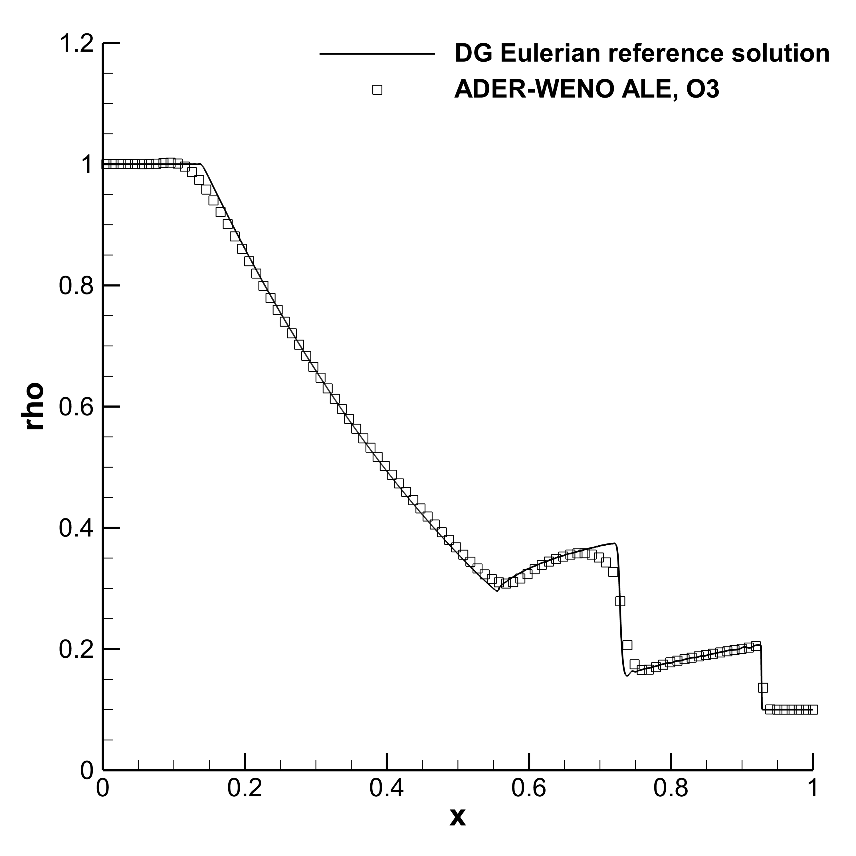
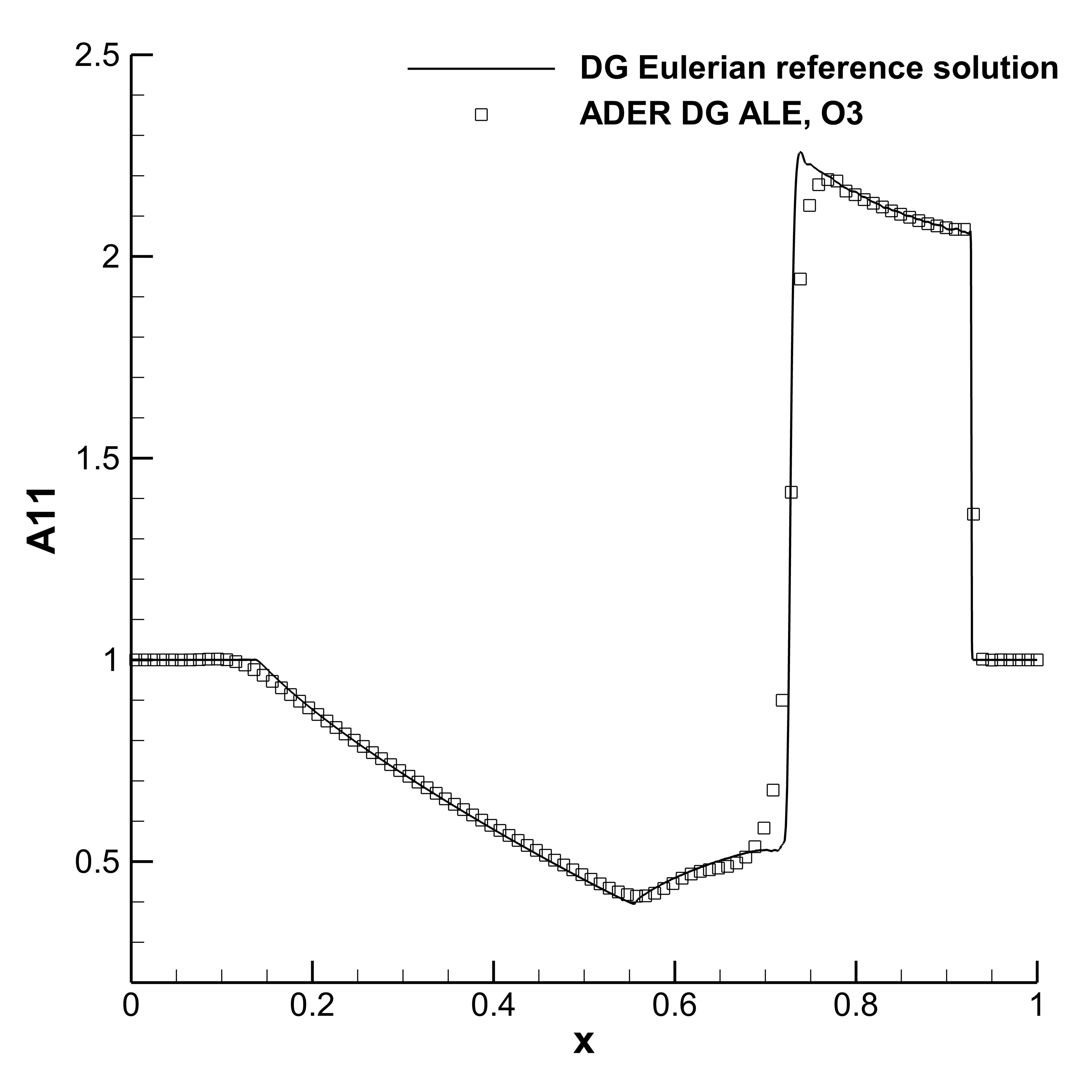
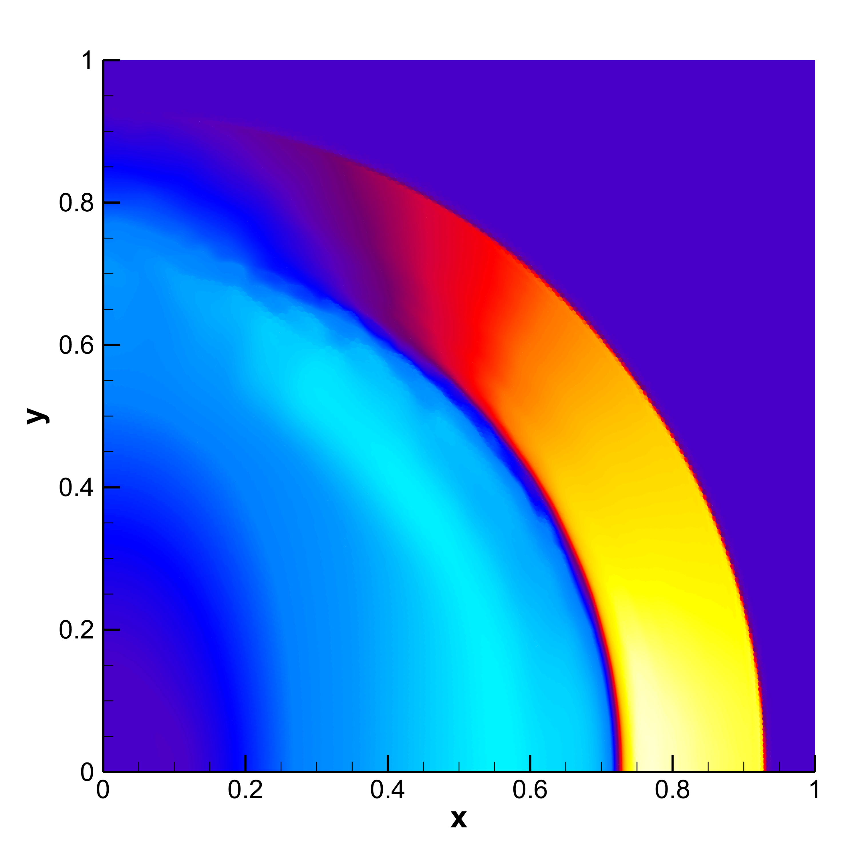
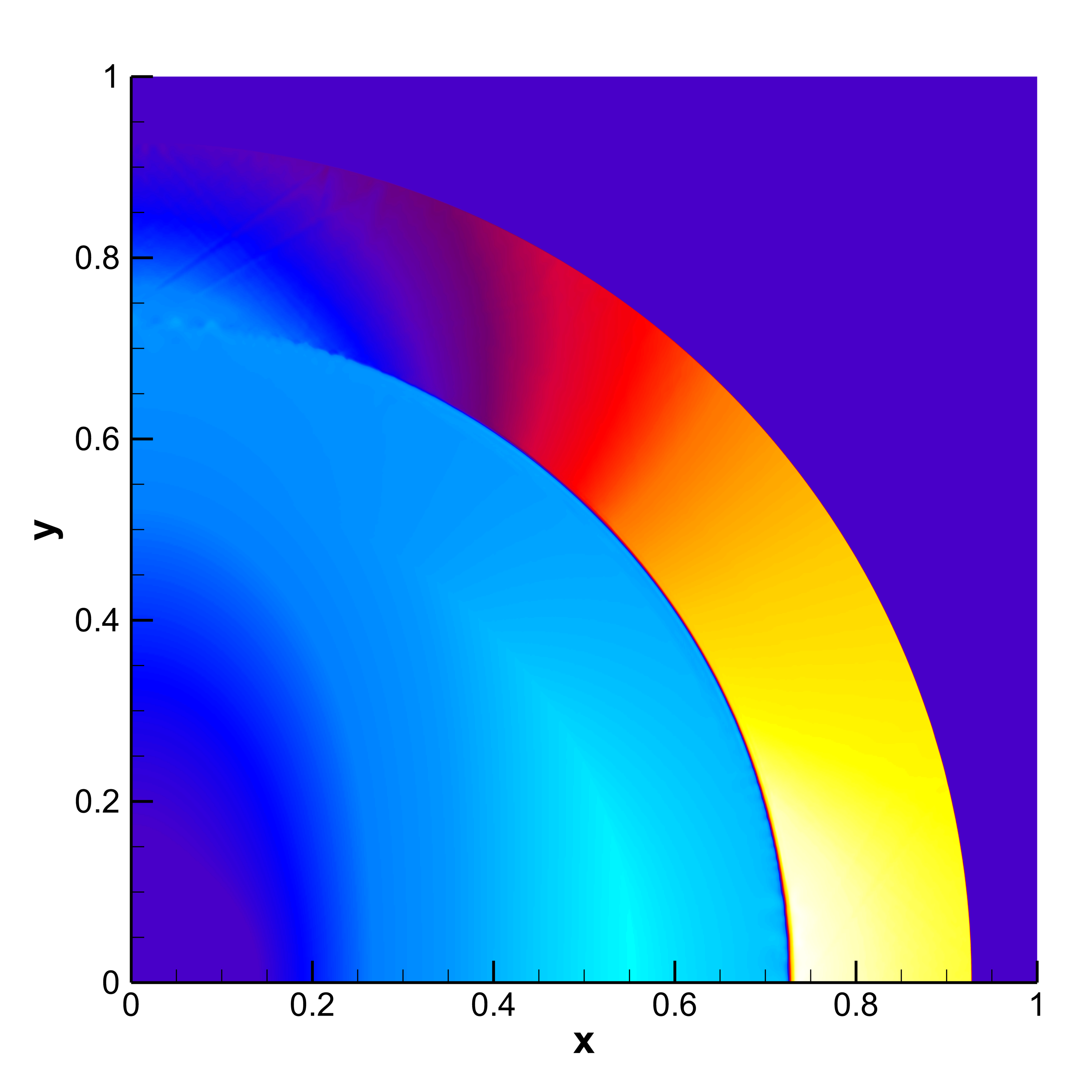
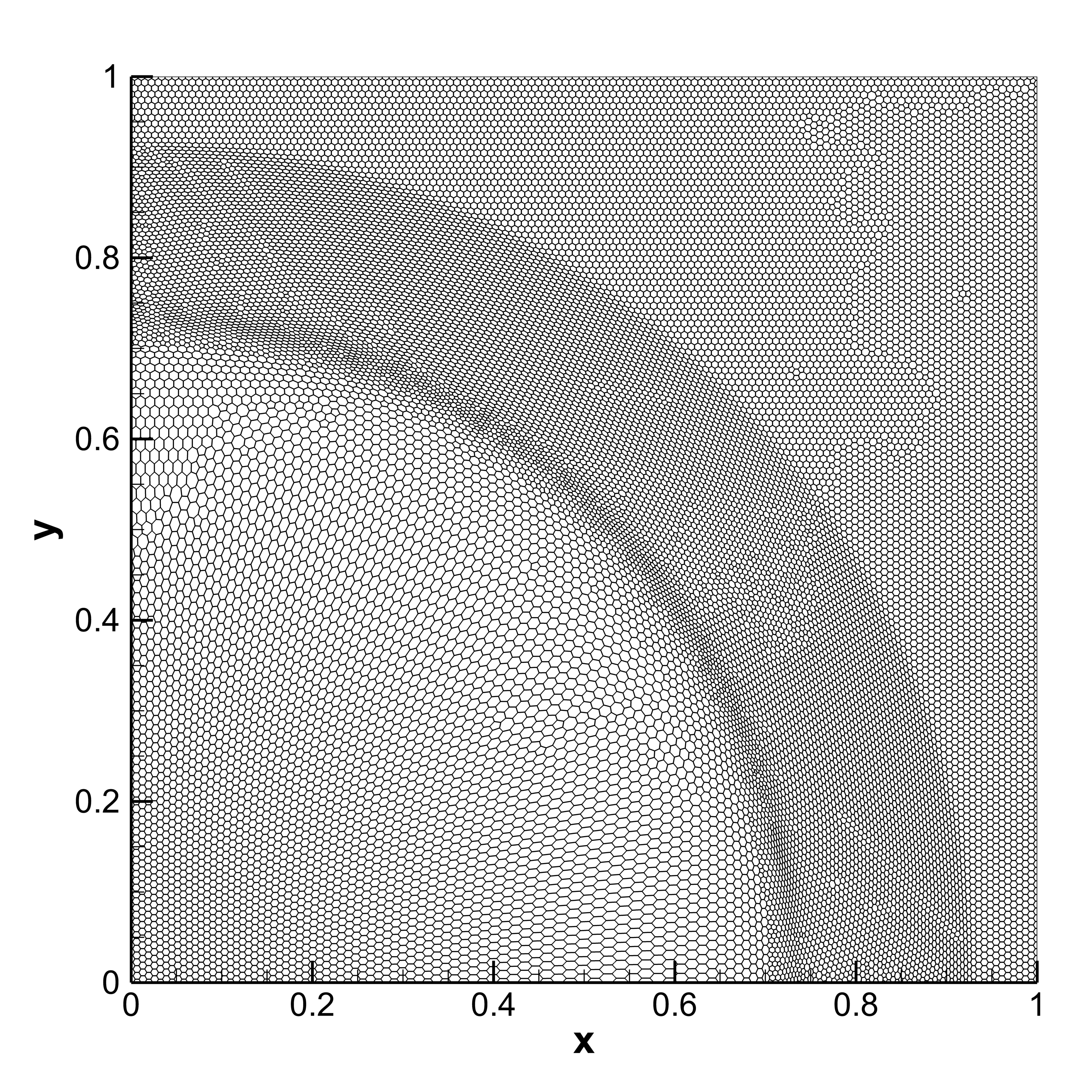
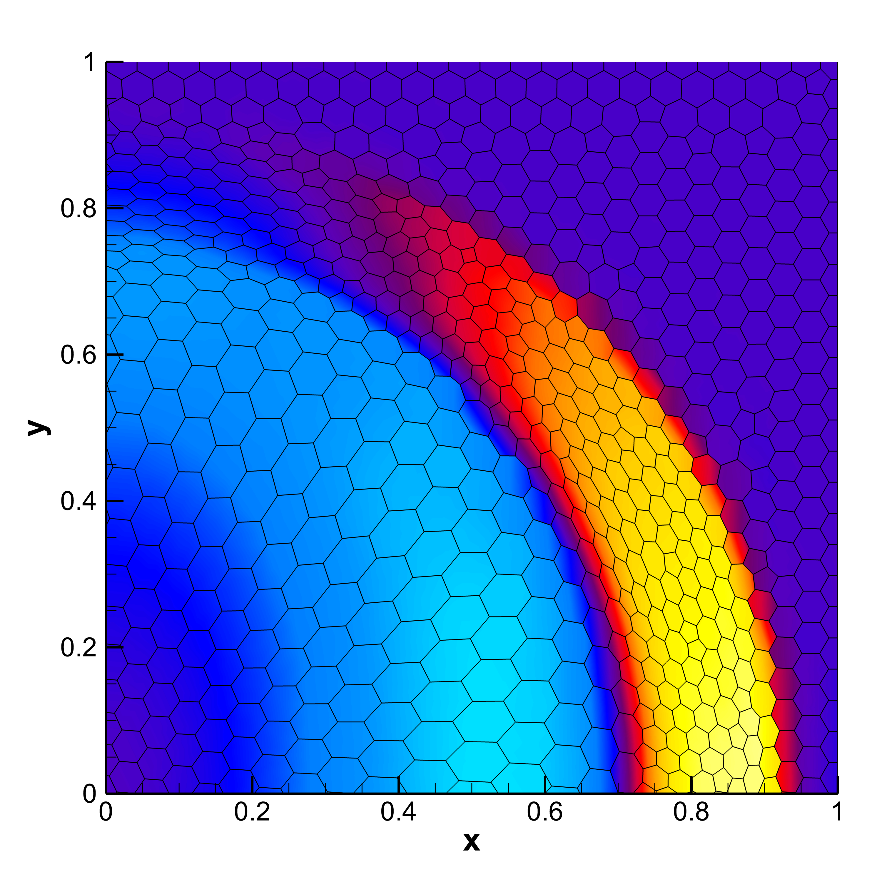
Figure 9: Simulation results for the explosion problem obtained with a third order ADER-WENO ALE finite volume scheme on a moving Voronoi grid composed of $82\,919$ cells and with a fourth order ADER-DG scheme on a Cartesian grid of size $512^{2}=262\,144$ ($4.2\times 10^{6}$ DOF). In the top row, two cuts of the solution along the $x$-axis are shown; in the middle row, from the left, the solution for $A_{11}$ obtained with the ADER-WENO ALE scheme and with the ADER-DG Eulerian scheme; in the bottom row, the Voronoi grid at the final simulation time and the results from the ADER-WENO ALE scheme on a coarser grid of $2\,727$ elements.

4.3 Rotor test problem

A second solid mechanics benchmark consists in the simulation of a plate on which a rotational impulse is initially impressed, in a circular region centered with respect to the computational domain. This rotor will initially move according to the rotational impulse, while emitting elastic waves which ultimately determine the formation of a set of concentric rings with alternating direction of rotation. The test is analogous to the rotor problem shown in [148], but with a weakened material in order to show stronger motion of the Voronoi grid.

The results of the third order ADER-WENO finite volume method on a moving Voronoi grid with variable connectivity, composed of $150\,561$ cells, are compared against a reference solution obtained with a fourth order ADER discontinuos Galerkin scheme on a very fine uniform Cartesian mesh counting $512\times 512$ elements, for a total of over four million spatial degrees of freedom.

The computational domain is the square $\Omega=[-1,1]\times[-1,1]$ and the final simulation time is set to $t=0.5$. With exception made for the velocity field, all variables are initially constant throughout the domain. Specifically we set $\alpha=1$, $\rho=1$, $p=1$, ${\bm{A}}={\bm{I}}$, ${\bm{J}}=\mathbf{0}$, while the velocity field is ${\bm{v}}=[-y/R,x/R,\ 0]$ if $r=\sqrt{x^{2}+y^{2}}\leq R$, and ${\bm{v}}=\mathbf{0}$ otherwise, that is, outside of the circle of radius $R=0.2$; this way, the initial tangential velocity at $r=R$ is one. The solid is taken to be elastic ($\tau_{1}\to\infty$), heat wave propagation is neglected ($c_{h}=0$), and the characteristic speed of shear waves is $c_{s}=0.25$. The constitutive law is chosen to be the stiffened-gas EOS with $\gamma=1.4$ and $p_{0}=0$. We can see in Figure 10 that, although some of the finer features are lost (specifically the small central counterclockwise-rotating ring) due to the lower resolution of the finite volume method on a coarser grid, the shear waves travel outwards with the correct velocity and the moving Voronoi finite volume simulation can be said to be in agreement with the high resolution discontinuous Galerkin results. Also in Figure 10, it is shown that the central region of the computational grid has undergone significant motion but thanks to the absence of constraints on the connectivity between elements, the Voronoi control volumes have not been stretched excessively as would instead happen for a similar moving unstructured grid, but with fixed connectivity.

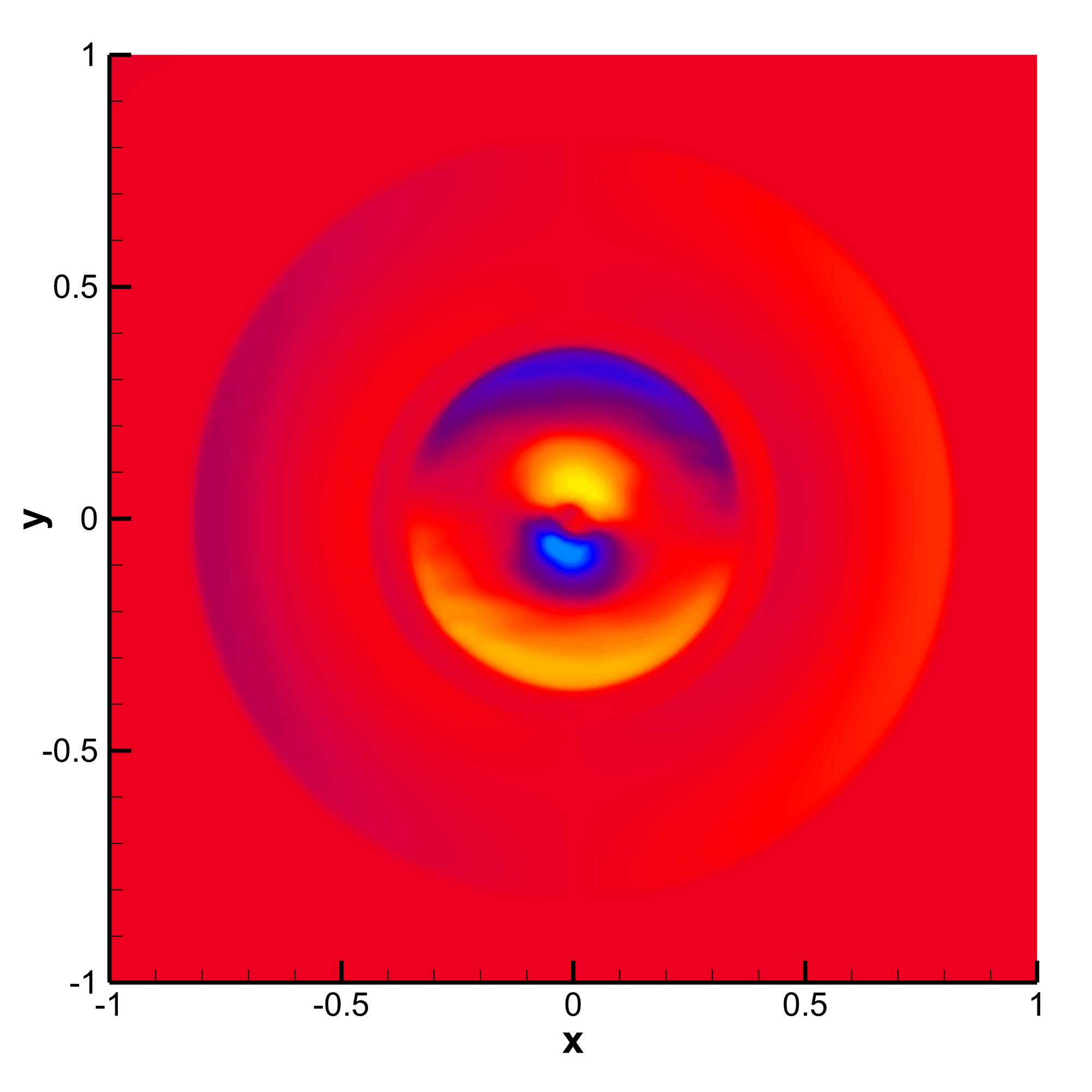
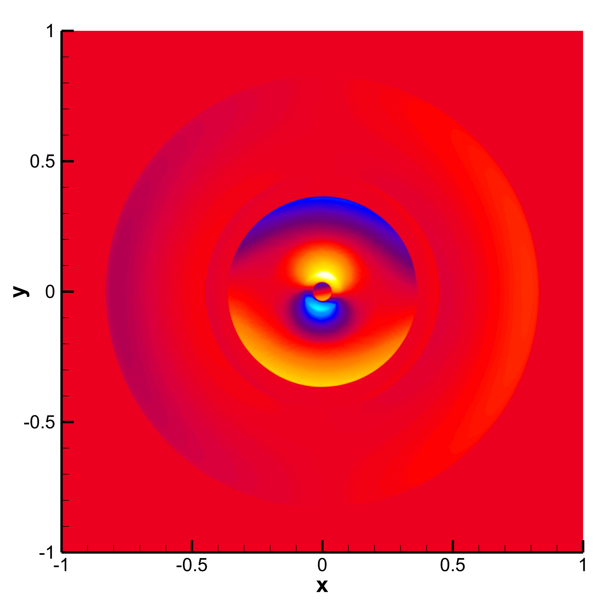
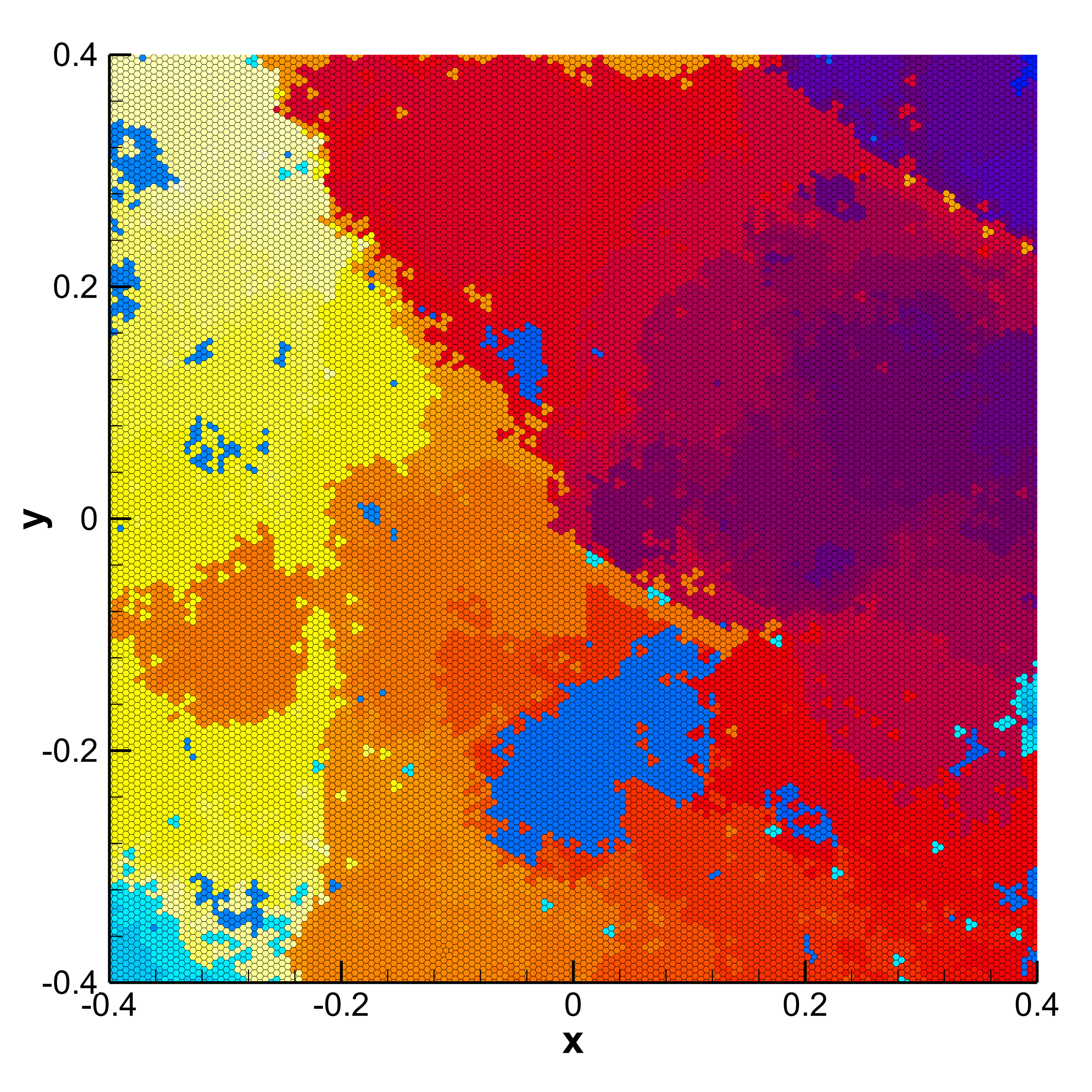
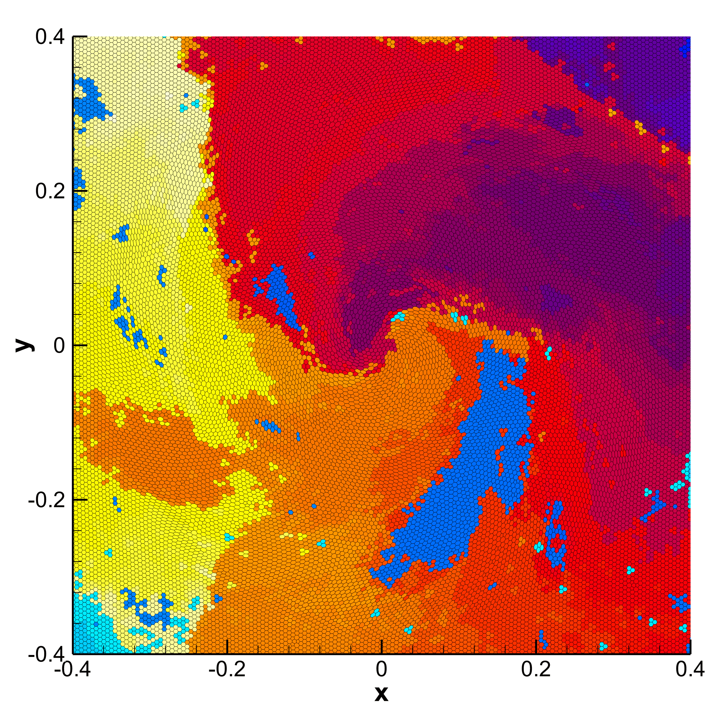
Figure 10: Simulation results for the solid rotor problem obtained from a third order ADER-WENO ALE finite volume scheme on a moving Voronoi grid composed of $150\,561$ cells and with a fourth order ADER-DG scheme on a cartesian grid of size $512^{2}=262\,144$ ($4.2\times 10^{6}$ DOF). In the top row, the solutions for the $u$ component of the velocity field are shown, on the left those obtained with the unstructured ADER-WENO ALE scheme on moving Voronoi meshes and on the right those of the ADER-DG scheme on a fixed Cartesian grid; in the bottom panels the cells are colored according to their mesh numbering to show the mesh motion between the beginning of the ALE simulation and the final time.

4.4 Elastic vibrations of a beryllium plate

The first benchmark for our new diffuse interface version of the GPR model consists in the purely elastic vibrations of a beryllium plate, subject to an initial velocity distribution, see for example [160, 138, 34, 27, 148] for a setup of the same test problem in the framework of Lagrangian and ALE schemes.

Unlike in the Lagrangian simulations, the computational domain considered here is larger and is set to $\Omega=[-5;5]\times[-2.5;2.5]$. The computational grid consists of $512\times 256$ uniform Cartesian cells with a characteristic mesh size of about $h=0.02$. We use a third order ADER-WENO finite volume scheme in the entire domain. The initial geometry of the beryllium bar is now simply defined by setting $\alpha(\mathbf{x},0)=1-\varepsilon$ inside the subdomain $\Omega_{b}=[-3,3]\times[-0.5,0.5]$, while the solid volume fraction function $\alpha$ is set to $\alpha(\mathbf{x},0)=\varepsilon$ elsewhere, with $\varepsilon=5\cdot 10^{-3}$. The initial velocity field inside $\Omega_{b}$ is imposed according to [34, 27, 148] as

$${\bm{v}}(\mathbf{x})=\left(0,A\omega\left\{C_{1}\left(\sinh(\Omega(x+3))+\sin(\Omega(x+3))\right)-S_{1}\left(\cosh(\Omega(x+3))+\cos(\Omega(x+3))\right)\right\},0\right),$$ (72)

with $\Omega=0.7883401241$, $\omega=0.2359739922$, $A=0.004336850425$, $S_{1}=57.64552048$ and $C_{1}=56.53585154$, while we simply set ${\bm{v}}=\mathbf{0}$ outside $\Omega_{b}$. For this test case we set $\varepsilon=5\cdot 10^{-3}$. The distortion field is initially set to ${\bm{A}}={\bm{I}}$. The material properties of Beryllium in the Mie-Grüneisen equation of state are taken as follows: $\rho_{0}=1.845$, $c_{0}=1.287$, $c_{s}=0.905$, $\Gamma=1.11$, and $s_{0}=1.124$. We furthermore neglect heat conduction and set $c_{h}=0$ and ${\bm{J}}=\mathbf{0}$.

Unlike in Lagrangian schemes, no boundary conditions need to be imposed on the surface of the bar. We simply use transmissive boundaries on $\partial\Omega$. The entire computational domain is initialized with the reference density for beryllium as $\rho(\mathbf{x},0)=\rho_{0}$, while the pressure is set to $p(\mathbf{x},0)=0$. The distortion field is initialized with ${\bm{A}}={\bm{I}}$. According to [34], the final time is set to $t_{f}=53.25$ so that it corresponds approximately to two complete flexural periods. The simulations are carried out with a third order ADER-WENO scheme on two uniform Cartesian meshes composed of $256\times 128$ and $512\times 256$ elements, respectively.

For the fine grid simulation in Figure 11, we present the temporal evolution of the color contour map of the volume fraction function $\alpha$, which represents the moving geometry of the bar. Here, dark gray color is used to indicate the regions with $\alpha>0.5$ and white color is used for the regions of $\alpha<0.5$. In the same figure, we also depict the pressure field in the region $\alpha>0.5$ at times $t=5$, $t=14$, $t=23$ and $t=28$. These time instants cover approximately one flexural period. The time evolution of the vertical velocity component $v(0,0,t)$ in the origin is depicted in Figure 12. For comparison, in the same figure we also show the results obtained on the coarse mesh for the same test problem with a fourth order ADER-DG scheme with second order TVD subcell finite volume limiter (red line).

Our computational results compare visually well against available reference solutions in the literature, see [160, 138, 34, 27, 148], which were all carried out with pure Lagrangian or Arbitrary-Lagrangian-Eulerian schemes on moving meshes, while here we use a diffuse interface approach on a fixed Cartesian grid.

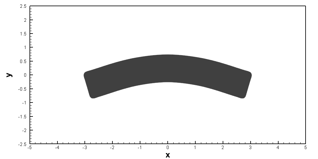
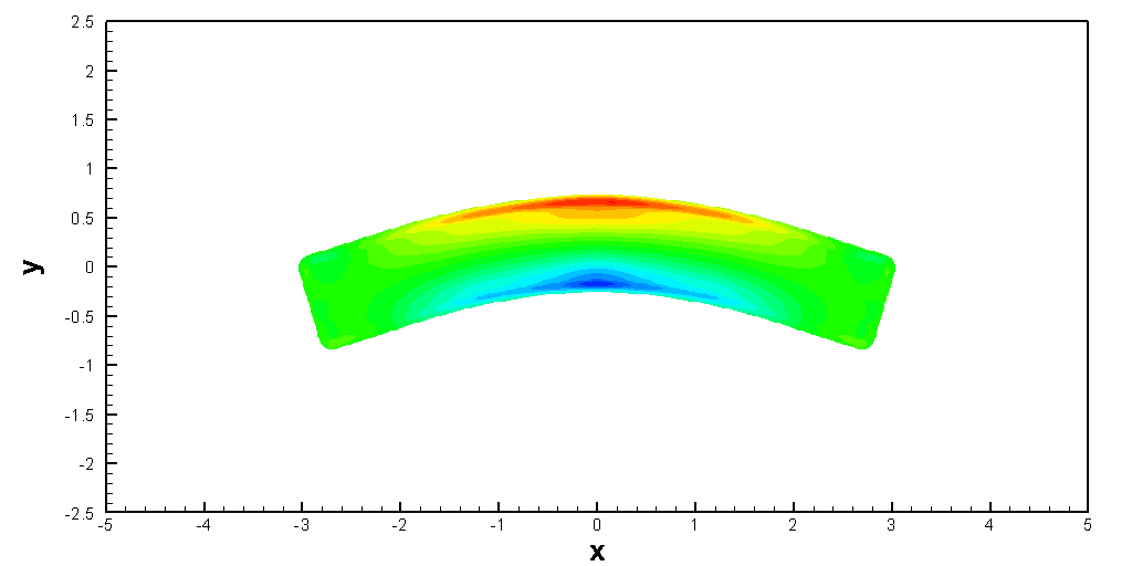
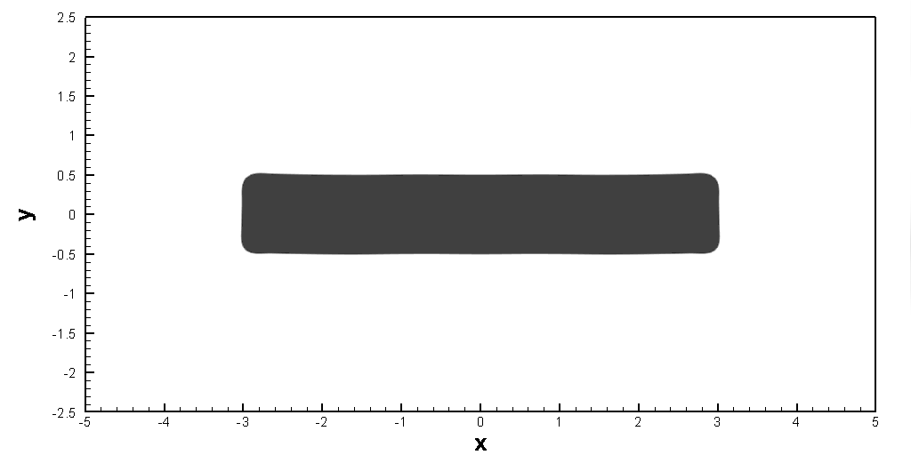
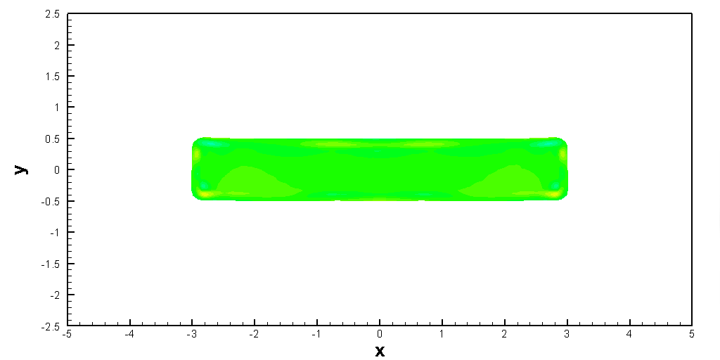
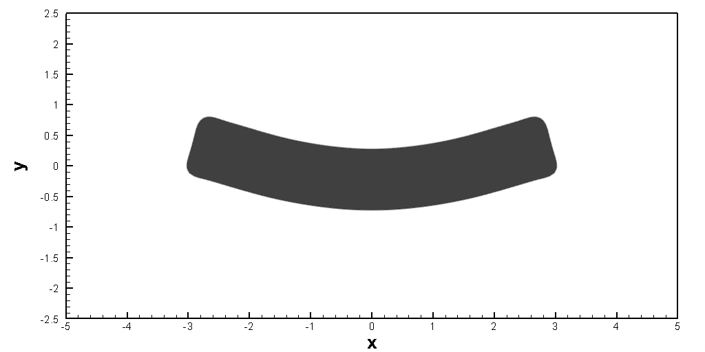
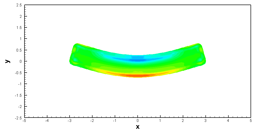
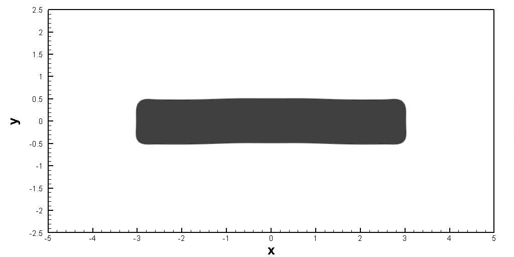
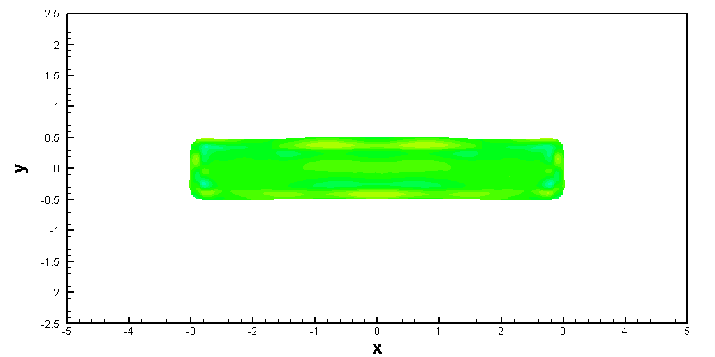
Figure 11: Vibration of an elastic beryllium plate. Temporal evolution of the volume fraction function $\alpha$ (left) and of the pressure field (right) at times $t=5$, $t=14$, $t=23$ and $t=28$, from top to bottom.

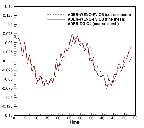
Figure 12: Temporal evolution of the vertical velocity component $v(0,0,t)$ obtained with a third order ADER-WENO scheme applied to the diffuse interface GPR model using two different mesh resolutions of $256\times 128$ elements (coarse mesh) and $512\times 256$ grid cells (fine mesh). For comparison, also a fourth order ADER-DG simulation on the coarse mesh is shown (red line).

4.5 Taylor bar impact problem

So far, we have only considered ideal elastic material, i.e. the limit case $\tau_{1}\to\infty$. In this section we consider also nonlinear elasto-plastic material behavior. Following [10, 11, 28, 148] we choose the relaxation time $\tau_{1}$ as a nonlinear function of an invariant of the stress tensor as follows:

$$\tau_{1}=\tau_{0}\left(\frac{\sigma_{0}}{\sigma}\right)^{m},$$ (73)

where $\tau_{0}$ is a constant characteristic relaxation time, $\sigma_{0}$ is the yield stress of the material and the von Mises stress $\sigma$ is given by

$$\sigma=\sqrt{\frac{1}{2}((\sigma_{11}-\sigma_{22})^{2}+(\sigma_{33}-\sigma_{11})^{2}+(\sigma_{33}-\sigma_{22})^{2}+6(\sigma_{12}^{2}+\sigma_{31}^{2}+\sigma_{32}^{2})}=\sqrt{\frac{3}{2}\mathring{\sigma}_{ij}\mathring{\sigma}_{ij}}.$$ (74)

In the formula (74) above, $\mathring{\sigma}_{ij}=\sigma_{ij}-\frac{1}{3}\sigma_{kk}\delta_{ij}$ is the stress deviator, i.e. the trace-free part of the stress tensor. The nonlinear relaxation time (73) tends to zero for $\sigma\gg\sigma_{0}$, while it tends to infinity for $\sigma\ll\sigma_{0}$.

The Taylor bar impact problem is a classical benchmark for an elasto-plastic aluminium projectile that hits a rigid solid wall, see [160, 138, 57, 28]. In this work the computational domain under consideration is $\Omega=[0,600]\times[-150,+150]$. The aluminium bar is initially located in the region $\Omega_{b}=[0,500]\times[-50,+50]$, where we set $\alpha=1-\varepsilon$, while in the rest of the computational domain we set $\alpha=\varepsilon$, with $\varepsilon=1\cdot 10^{-2}$.

The aluminium bar is described by the Mie-Grüneisen equation of state with parameters $\rho_{0}=2.785$, $c_{0}=0.533$, $c_{s}=0.305$, $\Gamma=2$ and $s=1.338$. The yield stress of aluminium is set to $\sigma_{0}=0.003$.

The projectile is initially moving with velocity ${\bm{v}}=(-0.015,0)$ towards a wall located at $x=0$. This velocity field is imposed within the subregion $\Omega_{b}$, while in the rest of the domain we set ${\bm{v}}=\mathbf{0}$. The remaining initial conditions are chosen as $\rho=\rho_{0}$, $p=p_{0}$, ${\bm{A}}={\bm{I}}$, ${\bm{J}}=\mathbf{0}$ and with the parameters $\tau_{0}=1$ and $m=20$ for the computation of the relaxation time (73). Unlike in Lagrangian schemes, we do not need to set any boundary conditions on the free surface of the moving bar. We only apply reflective slip wall boundary conditions on the wall in $x=0$. According to [138, 57, 28] the final time of the simulation is $t=5000$. The computational domain is discretized on a regular Cartesian grid composed of $512\times 256$ elements using a third order ADER-WENO finite volume scheme. As in [28] we employ a classical source splitting for the treatment of the stiff sources that arise in the regions of plastic deformations, i.e. when $\sigma\gg\sigma_{0}$. In Figure 13, we show the computational results at $t=1000$ and at the final time $t=5000$. The obtained solution is in agreement with the results presented in [138, 28, 148]. At time $t=5000$, we measure a final length of the projectile of $L_{f}=456$, which fits the results achieved in [138, 28] up to $2\%$.

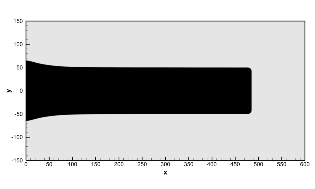
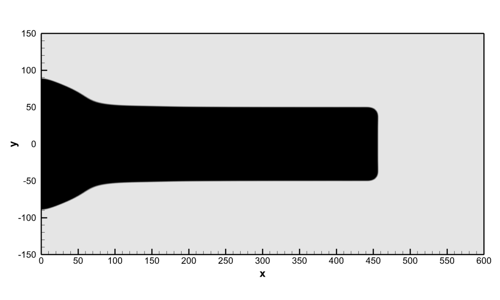
Figure 13: Geometry of the Taylor bar at time $t=1000$ (top) and at the final time $t=5000$ (bottom) obtained with a third order ADER-WENO finite volume scheme applied to the diffuse interface GPR model. We plot the contour colors of the volume fraction function $\alpha$, where black regions denote $\alpha>0.5$ and white regions $\alpha<0.5$.

4.6 Dambreak problem

In this last section on numerical test problems, we solve a two-dimensional dambreak problem with different relaxation times in order to show the entire range of potential applications of the GPR model. For this purpose, we also activate the gravity source term, setting the gravity vector to $\mathbf{g}=(0,-g)$ with $g=9.81$. The computational domain is chosen as $\Omega=[0,4]\times[0,2]$ and is discretized with a fourth order ADER discontinuous Galerkin finite element scheme with polynomial approximation degree $N=3$ and a posteriori subcell TVD finite volume limiter. Computations are run on a uniform Cartesian mesh composed of $128\times 64$ elements until the final time $t=0.5$. The initial condition is chosen as follows: we set $\rho=\rho_{0}$, ${\bm{v}}=\mathbf{0}$, ${\bm{A}}={\bm{I}}$ and ${\bm{J}}=\mathbf{0}$ in the entire computational domain. We impose the slip boundary condition on the bottom. In the subdomain $\Omega_{d}=[0,2]\times[0,1]$, we set $\alpha=1-\varepsilon$, and $p=\rho_{0}g(y-1)$, while in the rest of the domain we set $\alpha=\varepsilon$ and $p=0$. In this test problem we set $\varepsilon=10^{-2}$ and use a stiffened gas equation of state with parameters $\rho_{0}=1000$, $p_{0}=5\times 10^{4}$, $\gamma=2$, $c_{h}=0$ and a shear sound speed $c_{s}=6$. Simulations are run in three different regimes, only characterized by a different choice of the strain relaxation time $\tau_{1}$. In the first simulation, we set $\tau_{1}$ so that a kinematic viscosity $\nu=\mu/\rho_{0}=10^{-3}$ is reached in the stiff relaxation limit, i.e. the GPR model in this case describes an almost inviscid fluid. In the second simulation we choose $\tau_{1}$ so that $\nu=0.1$, i.e. a high viscosity Newtonian fluid behavior is reached. In the last simulation we set $\tau_{1}\to\infty$, i.e. the strain relaxation term is switched off so that an ideal elastic solid with low shear resistance is described, similar to a jelly-type medium. In all cases, we apply solid slip wall boundary conditions on the left and on the right of the computational domain, while on the right and upper boundary, transmissive boundary conditions are set. The temporal evolution of the volume fraction function $\alpha$, together with the coarse mesh used in this simulation, are depicted in Figure 14. The results for the almost inviscid fluid agree qualitatively well with those shown in [86, 59, 91] for nonhydrostatic dambreak problems. In order to corroborate this statement quantitatively, we now repeat the simulation with $\nu=10^{-3}$ using a fourth order ADER-DG scheme on a coarse AMR grid composed of only $32\times 16$ elements on the level zero grid. We then apply two levels of AMR refinement with refinement factor $\mathfrak{r}=3$, i.e. we employ a general space-tree, rather than a simple quad-tree. We note that the simulations on the AMR grid are run in combination with time-accurate local time stepping (LTS), which is trivial to implement in high order ADER-DG and ADER-FV schemes, due to their fully-discrete one-step nature. For details on LTS, see [72, 80, 60, 29]. As a reference solution of this almost inviscid flow problem, we solve the reduced barotropic and inviscid Baer-Nunziato model introduced in [59] and [91], using a third order ADER-WENO finite volume scheme on a very fine uniform Cartesian grid composed of $1024\times 512$ elements. The direct comparison of the two simulations at time $t=0.4$ is shown in Figure 15. Overall we can indeed note an excellent agreement between the behaviour of the diffuse interface GPR model in the stiff relaxation limit and the weakly compressible inviscid non-hydrostatic free surface flow model of [59, 91].

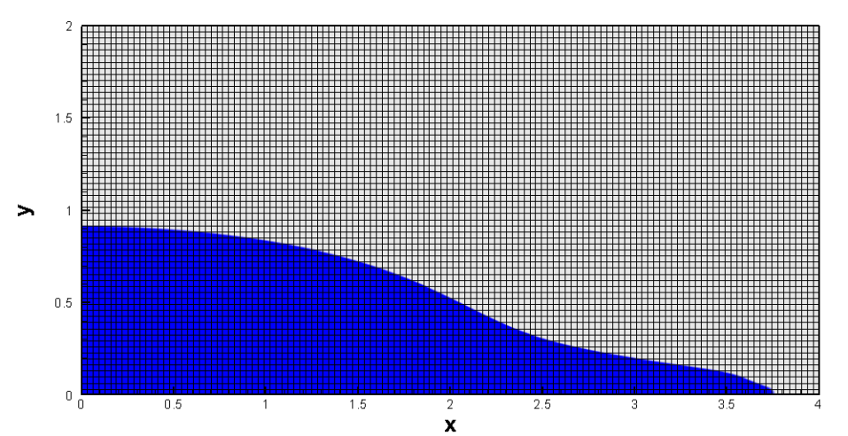
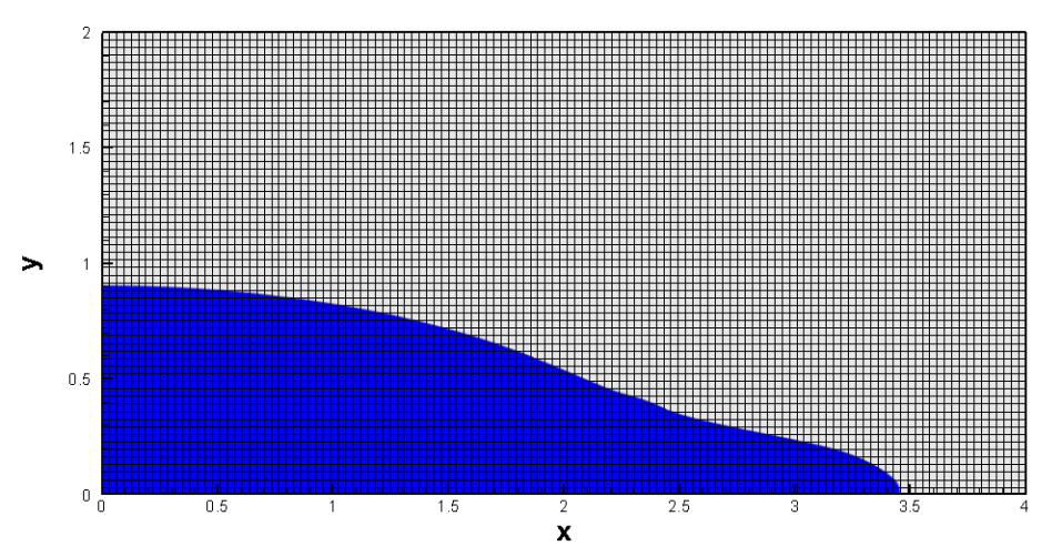
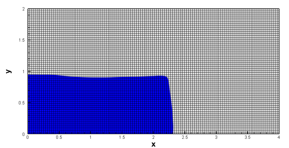
Figure 14: Dambreak problem at $t=0.5$, simulated with a fourth order ADER-DG scheme using different relaxation times. Top: low viscosity fluid (stiff relaxation limit) with $\nu=10^{-3}$. Center: high viscosity fluid with $\nu=10^{-1}$. Bottom: ideal elastic solid ($\tau_{1}\to\infty$) with low shear resistance.

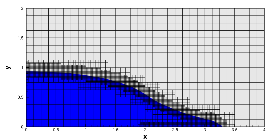
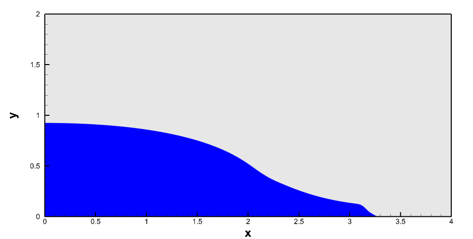
Figure 15: Dambreak problem at $t=0.4$, simulated with a fourth order ADER-DG scheme using a space-time adaptive Cartesian AMR mesh applied to the GPR model with with $\nu=10^{-3}$ (top panel), and reference solution, computed with a third order ADER-WENO finite volume scheme on a very fine uniform Cartesian grid, solving the inviscid and barotropic reduced Baer-Nunziato approach presented in [59, 91] (bottom panel).

5 Conclusions and Outlook

In the first part of this paper we have provided a review of the ADER approach, whose development started about 20 years ago with the seminal works of [178, 140] and [174, 180] in the context of approximate solvers for the generalized Riemann problem (GPR). The ADER method provides fully discrete explicit one-step schemes that are in principle arbitrary high order accurate in both space and time. The most recent developments include ADER schemes for stiff source terms, as well as ADER finite volume and discontinuous Galerkin finite element schemes on fixed and moving meshes, which are all based on a space-time predictor-corrector approach. The fact that ADER schemes are fully discrete makes the implementation of time accurate local time stepping (LTS) particularly simple, both on adaptive Cartesian AMR meshes [80], as well as in the context of Lagrangian schemes on moving grids [60, 29]. The fully discrete space-time formulation also allows the treatment of topology changes during one time step in a very natural way [90]. In the second part of the paper we have then shown several applications of high order ADER finite volume and discontinuous Galerkin finite element schemes to the novel unified hyperbolic model of continuum mechanics (GPR model) proposed by Godunov, Peshkov and Romenski [98, 150, 76]. The presented test problems cover the entire range of continuum mechanics, from ideal elastic solids over plastic solids to viscous fluids. The use of a diffuse interface approach allows also to simulate moving boundary problems on fixed Cartesian meshes. Future developments will concern the extension of the mathematical model to non-Newtonian fluids [118] and to free surface flows with surface tension, see [161, 44], as well as to the conservative multi-phase model of [158, 157]. In future work we will also consider the use of novel all speed schemes [1] and semi-implicit space-time discontinuous Galerkin finite element schemes [172, 116, 37] for the diffuse interface version of the GPR model used in this paper.

Conflict of Interest Statement

The authors declare that the research was conducted in the absence of any commercial or financial relationships that could be construed as a potential conflict of interest.

Author Contributions

The governing PDE system was developed by IP. The numerical method and the computer codes were developed by MD, EG and SC. The test problems were computed by MD, EG and SC. The analysis of the method was performed by SB. All authors discussed the results and contributed to the final manuscript.

Funding

The research presented in this paper has been financed by the European Union’s Horizon 2020 Research and Innovation Programme under the project ExaHyPE, grant agreement number no. 671698 (call FET-HPC-1-2014).

S.B. has also received funding by INdAM (Istituto Nazionale di Alta Matematica, Italy) under a Post-doctoral grant of the research project Progetto premiale FOE 2014-SIES.

S.C. acknowledges the financial support received by the Deutsche Forschungsgemeinschaft (DFG) under the project Droplet Interaction Technologies (DROPIT), grant no. GRK 2160/1.

M.D. also acknowledges the financial support received from the Italian Ministry of Education, University and Research (MIUR) in the frame of the Departments of Excellence Initiative 2018–2022 attributed to DICAM of the University of Trento (grant L. 232/2016) and in the frame of the PRIN 2017 project. M.D. has also received funding from the University of Trento via the Strategic Initiative Modeling and Simulation.

E.G. has also been financed by a national mobility grant for young researchers in Italy, funded by GNCS-INdAM and acknowledges the support given by the University of Trento through the UniTN Starting Grant initiative.

References

- [1] E. Abbate, A. Iollo, and G. Puppo. An asymptotic-preserving all-speed scheme for fluid dynamics and nonlinear elasticity. SIAM Journal on Scientific Computing, 41:A2850–A2879, 2019.
- [2] B. Andreotti, Y. Forterre, and O. Pouliquen. Granular Media: Between Fluid and Solid. Cambridge University Press, 2013.
- [3] N. J. Balmforth, I. A. Frigaard, and G. Ovarlez. Yielding to Stress : Recent Developments in Viscoplastic Fluid Mechanics. Annual Review of Fluid Mechanics, 46(August):121–146, 2014.
- [4] D. Balsara, C. Altmann, C. Munz, and M. Dumbser. A sub-cell based indicator for troubled zones in RKDG schemes and a novel class of hybrid RKDG+HWENO schemes. Journal of Computational Physics, 226:586–620, 2007.
- [5] D. Balsara and M. Dumbser. Divergence-free MHD on unstructured meshes using high order finite volume schemes based on multidimensional Riemann solvers. Journal of Computational Physics, pages 687–715, 2015.
- [6] D. Balsara, M. Dumbser, and R. Abgrall. Multidimensional HLLC Riemann Solver for Unstructured Meshes - With Application to Euler and MHD Flows. Journal of Computational Physics, 261:172–208, 2014.
- [7] D. Balsara and C. Shu. Monotonicity preserving weighted essentially non-oscillatory schemes with increasingly high order of accuracy. Journal of Computational Physics, 160:405–452, 2000.
- [8] S. Banach. Sur les opérations dans les ensembles abstraits et leur application aux équations intégrales. Fund. math, 3(1):133–181, 1922.
- [9] T. Barth and D. Jespersen. The design and application of upwind schemes on unstructured meshes. AIAA Paper 89-0366, pages 1–12, 1989.
- [10] P. Barton, D. Drikakis, and E. Romenski. An Eulerian finite-volume scheme for large elastoplastic deformations in solids. International Journal for Numerical Methods in Engineering, 81:453–484, 2010.
- [11] P. Barton, B. Obadia, and D. Drikakis. A conservative level-set based method for compressible solid/fluid problems on fixed grids. Journal of Computational Physics, 230:7867–7890, 2011.
- [12] P. T. Barton. An interface-capturing Godunov method for the simulation of compressible solid-fluid problems. Journal of Computational Physics, 390:25–50, 2019.
- [13] M. Ben-Artzi and J. Falcovitz. A second-order Godunov-type scheme for compressible fluid dynamics. Journal of Computational Physics, 55:1–32, 1984.
- [14] M. Ben-Artzi and J. Falcovitz. Generalized Riemann problems in computational fluid dynamics. Number 11 in Cambridge Monographs on Applied and Computational Mathematics. Cambridge University Press, Cambridge, UK, 2003.
- [15] M. Ben-Artzi, J. Li, and G. Warnecke. A direct eulerian GRP scheme for compressible fluid flows. Journal of Computational Physics, 218:19–43, 2006.
- [16] C. Berthon. Why the MUSCL-Hancock scheme is L1-stable. Numer. Math., 104:27–46, 2006.
- [17] S. Billett and E. Toro. On the accuracy and stability of explicit schemes for multidimensional linear homogeneous advection equations. Journal of Computational Physics, 131:247–250, 1997.
- [18] M. Bonazzoli, E. Gaburro, V. Dolean, and F. Rapetti. High order edge finite element approximations for the time-harmonic maxwell’s equations. In 2014 IEEE Conference on Antenna Measurements & Applications (CAMA), pages 1–4. IEEE, 2014.
- [19] W. Boscheri. An efficient high order direct ALE ADER finite volume scheme with a posteriori limiting for hydrodynamics and magnetohydrodynamics. International Journal for Numerical Methods in Fluids, 134-135:111–129, 2016.
- [20] W. Boscheri, D. Balsara, and M. Dumbser. Lagrangian ADER-WENO finite volume schemes on unstructured triangular meshes based on genuinely multidimensional HLL riemann solvers. Journal of Computational Physics, 267:112–138, 2014.
- [21] W. Boscheri and M. Dumbser. Arbitrary–Lagrangian–Eulerian One–Step WENO Finite Volume Schemes on Unstructured Triangular Meshes. Communications in Computational Physics, 14:1174–1206, 2013.
- [22] W. Boscheri and M. Dumbser. A direct Arbitrary-Lagrangian-Eulerian ADER-WENO finite volume scheme on unstructured tetrahedral meshes for conservative and non-conservative hyperbolic systems in 3D. Journal of Computational Physics, 275:484 – 523, 2014.
- [23] W. Boscheri and M. Dumbser. An efficient quadrature-free formulation for high order Arbitrary-Lagrangian-Eulerian ADER-WENO finite volume schemes on unstructured meshes. Journal of Scientific Computing, 66:240–274, 2016.
- [24] W. Boscheri and M. Dumbser. High order accurate direct Arbitrary-Lagrangian-Eulerian ADER-WENO finite volume schemes on moving curvilinear unstructured meshes. Computers and Fluids, 136:48–66, 2016.
- [25] W. Boscheri and M. Dumbser. Arbitrary–Lagrangian–Eulerian Discontinuous Galerkin schemes with a posteriori subcell finite volume limiting on moving unstructured meshes. Journal of Computational Physics, 346:449–479, 2017.
- [26] W. Boscheri, M. Dumbser, and D. Balsara. High Order Lagrangian ADER-WENO Schemes on Unstructured Meshes – Application of Several Node Solvers to Hydrodynamics and Magnetohydrodynamics. International Journal for Numerical Methods in Fluids, 76:737–778, 2014.
- [27] W. Boscheri, M. Dumbser, and R. Loubere. Cell centered direct Arbitrary-Lagrangian-Eulerian ADER-WENO finite volume schemes for nonlinear hyperelasticity. Computers and Fluids, 134–135:111–129, 2016.
- [28] W. Boscheri, M. Dumbser, and R. Loubère. Cell centered direct Arbitrary-Lagrangian-Eulerian ADER-WENO finite volume schemes for nonlinear hyperelasticity. Computers and Fluids, 134-135:111–129, 2016.
- [29] W. Boscheri, M. Dumbser, and O. Zanotti. High order cell-centered lagrangian-type finite volume schemes with time-accurate local time stepping on unstructured triangular meshes. Journal of Computational Physics, 291:120–150, 2014.
- [30] W. Boscheri and R. Loubère. High order accurate direct Arbitrary-Lagrangian-Eulerian ADER-MOOD finite volume schemes for non-conservative hyperbolic systems with stiff source terms. Communications in Computational Physics, 21:271–312, 2017.
- [31] W. Boscheri, R. Loubère, and M. Dumbser. Direct Arbitrary-Lagrangian-Eulerian ADER-MOOD finite volume schemes for multidimensional hyperbolic conservation laws. Journal of Computational Physics, 292:56–87, 2015.
- [32] W. Boscheri, M. Semplice, and M. Dumbser. Central WENO Subcell Finite Volume Limiters for ADER Discontinuous Galerkin Schemes on Fixed and Moving Unstructured Meshes. Communications in Computational Physics, 25:311–346, 2019.
- [33] H. Bungartz, M. Mehl, T. Neckel, and T. Weinzierl. The PDE framework Peano applied to fluid dynamics: An efficient implementation of a parallel multiscale fluid dynamics solver on octree-like adaptive Cartesian grids. Computational Mechanics, 46:103–114, 2010.
- [34] D. Burton, N. Morgan, T. Carney, and M. Kenamond. Reduction of dissipation in Lagrange cell-centered hydrodynamics (CCH) through corner gradient reconstruction (CGR). Journal of Computational Physics, 299:229–280, 2015.
- [35] S. Busto. Contributions to the numerical solution of heterogeneous fluid mechanics models. PhD thesis, Universidade de Santiago de Compostela, 2018.
- [36] S. Busto, J. Ferrín, E. Toro, and M. Vázquez-Cendón. A projection hybrid high order finite volume/finite element method for incompressible turbulent flows. Journal of Computational Physics, 353:169 – 192, 2018.
- [37] S. Busto, M. Tavelli, W. Boscheri, and M. Dumbser. Efficient high order accurate staggered semi-implicit discontinuous Galerkin methods for natural convection problems. Computers & Fluids, 198:104399, 2020.
- [38] S. Busto, E. F. Toro, and M. E. Vázquez-Cendón. Design and analysis of ADER-type schemes for model advection–diffusion–reaction equations. Journal of Computational Physics, 327:553–575, 2016.
- [39] M. Campos-Pinto, F. Charles, B. Després, and M. Herda. A projection algorithm on the set of polynomials with two bounds. arXiv preprint arXiv:1905.05546, 2019.
- [40] C. Castro, M. Käser, and E. Toro. Space–time adaptive numerical methods for geophysical applications. Philosophical Transactions of the Royal Society A: Mathematical, Physical and Engineering Sciences, 367(1907):4613–4631, 2009.
- [41] C. C. Castro and E. F. Toro. Solvers for the high-order Riemann problem for hyperbolic balance laws. Journal of Computational Physics, 227:2481–2513, 2008.
- [42] M. Castro, J. Gallardo, and C. Parés. High-order finite volume schemes based on reconstruction of states for solving hyperbolic systems with nonconservative products. Applications to shallow-water systems. Mathematics of Computation, 75:1103–1134, 2006.
- [43] J. Cesenek, M. Feistauer, J. Horacek, V. Kucera, and J. Prokopova. Simulation of compressible viscous flow in time–dependent domains. Applied Mathematics and Computation, 219:7139–7150, 2013.
- [44] S. Chiocchetti, I. Peshkov, S. Gavrilyuk, and M. Dumbser. High order ADER schemes and GLM curl cleaning for a first order hyperbolic formulation of compressible flow with surface tension. Journal of Computational Physics, 2020. arXiv:2002.08818.
- [45] S. Clain, S. Diot, and R. Loubère. A high-order finite volume method for systems of conservation laws—multi-dimensional optimal order detection (MOOD). Journal of Computational Physics, 230(10):4028 – 4050, 2011.
- [46] B. Cockburn and C. W. Shu. The Runge-Kutta discontinuous Galerkin method for conservation laws V: multidimensional systems. Journal of Computational Physics, 141:199–224, 1998.
- [47] P. Colella. A direct eulerian muscl scheme for gas dynamics. SIAM Journal on Scientific and Statistical Computing, 6(1):104–117, 1985.
- [48] C. Contarino, E. Toro, G. Montecinos, R. Borsche, and J. Kall. Junction-generalized Riemann problem for stiff hyperbolic balance laws in networks: An implicit solver and ADER schemes. Journal of Computational Physics, 315:409 – 433, 2016.
- [49] I. Cravero, G. Puppo, M. Semplice, and G. Visconti. CWENO: uniformly accurate reconstructions for balance laws. Mathematics of Computation, 87(312):1689–1719, 2018.
- [50] G. Dal Maso, P. LeFloch, and F. Murat. Definition and weak stability of nonconservative products. J. Math. Pures Appl., 74:483–548, 1995.
- [51] A. de Brauer, A. Iollo, and T. Milcent. A Cartesian Scheme for Compressible Multimaterial Hyperelastic Models with Plasticity. Communications in Computational Physics, 22(05):1362–1384, 2017.
- [52] J. N. de la Rosa and C.-D. Munz. Hybrid dg/fv schemes for magnetohydrodynamics and relativistic hydrodynamics. Computer Physics Communications, 222:113 – 135, 2018.
- [53] R. Dematté, V. A. Titarev, G. I. Montecinos, and E. F. Toro. ADER methods for hyperbolic equations with a time-reconstruction solver for the generalized Riemann problem: the scalar case. Communications on Applied Mathematics and Computation, 2019.
- [54] B. Després. Polynomials with bounds and numerical approximation. Numerical Algorithms, 76(3):829–859, 2017.
- [55] S. Diot, S. Clain, and R. Loubère. Improved detection criteria for the multi-dimensional optimal order detection (MOOD) on unstructured meshes with very high-order polynomials. Computers and Fluids, 64:43 – 63, 2012.
- [56] S. Diot, R. Loubère, and S. Clain. The MOOD method in the three-dimensional case: Very-high-order finite volume method for hyperbolic systems. International Journal of Numerical Methods in Fluids, 73:362–392, 2013.
- [57] V. A. Dobrev, T. V. Kolev, and R. N. Rieben. High order curvilinear finite elements for elastic–plastic lagrangian dynamics. Journal of Computational Physics, 257:1062–1080, 2014.
- [58] M. Dumbser. Arbitrary high order PNPM schemes on unstructured meshes for the compressible Navier–Stokes equations. Computers & Fluids, 39:60–76, 2010.
- [59] M. Dumbser. A simple two–phase method for the simulation of complex free surface flows. Computer Methods in Applied Mechanics and Engineering, 200:1204–1219, 2011.
- [60] M. Dumbser. Arbitrary-Lagrangian-Eulerian ADER-WENO Finite Volume Schemes with Time-Accurate Local Time Stepping for Hyperbolic Conservation Laws. Computational Methods in Applied Mechanics and Engineering, 280:57–83, 2014.
- [61] M. Dumbser, D. Balsara, E. Toro, and C. Munz. A unified framework for the construction of one-step finite–volume and discontinuous Galerkin schemes. Journal of Computational Physics, 227:8209–8253, 2008.
- [62] M. Dumbser, W. Boscheri, M. Semplice, and G. Russo. Central weighted ENO schemes for hyperbolic conservation laws on fixed and moving unstructured meshes. SIAM Journal on Scientific Computing, 39(6):A2564–A2591, 2017.
- [63] M. Dumbser, M. Castro, C. Parés, and E. Toro. ADER schemes on unstructured meshes for non–conservative hyperbolic systems: Applications to geophysical flows. Computers and Fluids, 38:1731––1748, 2009.
- [64] M. Dumbser, C. Enaux, and E. Toro. Finite volume schemes of very high order of accuracy for stiff hyperbolic balance laws. Journal of Computational Physics, 227:3971–4001, 2008.
- [65] M. Dumbser, F. Fambri, E. Gaburro, and A. Reinarz. On glm curl cleaning for a first order reduction of the ccz4 formulation of the einstein field equations. Journal of Computational Physics, 404:109088, 2020.
- [66] M. Dumbser, F. Fambri, M. Tavelli, M. Bader, and T. Weinzierl. Efficient implementation of ADER discontinuous Galerkin schemes for a scalable hyperbolic pde engine. Axioms, 7(3):63, 2018.
- [67] M. Dumbser, F. Guercilena, S. Köppel, L. Rezzolla, and O. Zanotti. Conformal and covariant Z4 formulation of the Einstein equations: strongly hyperbolic first–order reduction and solution with discontinuous Galerkin schemes. Physical Review D, 97:084053, 2018.
- [68] M. Dumbser, A. Hidalgo, M. Castro, C. Parés, and E. Toro. FORCE schemes on unstructured meshes II: Non–conservative hyperbolic systems. Computer Methods in Applied Mechanics and Engineering, 199:625–647, 2010.
- [69] M. Dumbser, A. Hidalgo, and O. Zanotti. High Order Space-Time Adaptive ADER-WENO Finite Volume Schemes for Non-Conservative Hyperbolic Systems. Computer Methods in Applied Mechanics and Engineering, 268:359–387, 2014.
- [70] M. Dumbser and M. Käser. Arbitrary high order non-oscillatory finite volume schemes on unstructured meshes for linear hyperbolic systems. Journal of Computational Physics, 221:693–723, 2007.
- [71] M. Dumbser, M. Käser, V. Titarev, and E. Toro. Quadrature-free non-oscillatory finite volume schemes on unstructured meshes for nonlinear hyperbolic systems. Journal of Computational Physics, 226:204–243, 2007.
- [72] M. Dumbser, M. Käser, and E. F. Toro. An arbitrary high order discontinuous Galerkin method for elastic waves on unstructured meshes V: Local time stepping and -adaptivity. Geophysical Journal International, 171:695–717, 2007.
- [73] M. Dumbser and R. Loubère. A simple robust and accurate a posteriori sub–cell finite volume limiter for the discontinuous Galerkin method on unstructured meshes. Journal of Computational Physics, 319:163–199, 2016.
- [74] M. Dumbser and C. Munz. Building blocks for arbitrary high order discontinuous Galerkin schemes. Journal of Scientific Computing, 27:215–230, 2006.
- [75] M. Dumbser, I. Peshkov, and E. Romenski. A Unified Hyperbolic Formulation for Viscous Fluids and Elastoplastic Solids. In C. Klingenberg and M. Westdickenberg, editors, Theory, Numerics and Applications of Hyperbolic Problems II. HYP 2016, volume 237 of Springer Proceedings in Mathematics and Statistics, pages 451–463. Springer International Publishing, 2018.
- [76] M. Dumbser, I. Peshkov, E. Romenski, and O. Zanotti. High order ADER schemes for a unified first order hyperbolic formulation of continuum mechanics: Viscous heat-conducting fluids and elastic solids. Journal of Computational Physics, 314:824–862, 2016.
- [77] M. Dumbser, I. Peshkov, E. Romenski, and O. Zanotti. High order ADER schemes for a unified first order hyperbolic formulation of Newtonian continuum mechanics coupled with electro-dynamics. Journal of Computational Physics, 348:298–342, 2017.
- [78] M. Dumbser and E. F. Toro. A simple extension of the Osher Riemann solver to non-conservative hyperbolic systems. Journal of Scientific Computing, 48:70–88, 2011.
- [79] M. Dumbser and O. Zanotti. Very high order PNPM schemes on unstructured meshes for the resistive relativistic MHD equations. Journal of Computational Physics, 228:6991–7006, 2009.
- [80] M. Dumbser, O. Zanotti, A. Hidalgo, and D. Balsara. ADER-WENO Finite Volume Schemes with Space-Time Adaptive Mesh Refinement. Journal of Computational Physics, 248:257–286, 2013.
- [81] M. Dumbser, O. Zanotti, R. Loubère, and S. Diot. A posteriori subcell limiting of the discontinuous Galerkin finite element method for hyperbolic conservation laws. Journal of Computational Physics, 278:47–75, 2014.
- [82] F. Fambri, M. Dumbser, S. Köppel, L. Rezzolla, and O. Zanotti. ADER discontinuous Galerkin schemes for general-relativistic ideal magnetohydrodynamics. Monthly Notices of the Royal Astronomical Society, 477:4543–4564, 2018.
- [83] F. Fambri, M. Dumbser, and O. Zanotti. Space-time adaptive ADER-DG schemes for dissipative flows: Compressible Navier-Stokes and resistive MHD equations. Computer Physics Communications, 220:297–318, 2017.
- [84] N. Favrie and S. Gavrilyuk. Diffuse interface model for compressible fluid - Compressible elastic-plastic solid interaction. Journal of Computational Physics, 231(7):2695–2723, 2012.
- [85] N. Favrie, S. Gavrilyuk, and R.Saurel. Solid–fluid diffuse interface model in cases of extreme deformations. Journal of Computational Physics, 228:6037–6077, 2009.
- [86] A. Ferrari, M. Dumbser, E. Toro, and A. Armanini. A new 3D parallel SPH scheme for free surface flows. Computers & Fluids, 38:1203–1217, 2009.
- [87] M. Francois, A. Sun, W. King, N. Henson, D. Tourret, C. Bronkhorst, N. Carlson, C. Newman, T. Haut, J. Bakosi, J. Gibbs, V. Livescu, S. Vander Wiel, A. Clarke, M. Schraad, T. Blacker, H. Lim, T. Rodgers, S. Owen, F. Abdeljawad, J. Madison, A. Anderson, J.-L. Fattebert, R. Ferencz, N. Hodge, S. Khairallah, and O. Walton. Modeling of additive manufacturing processes for metals: Challenges and opportunities. Current Opinion in Solid State and Materials Science, 21(4):198–206, 2017.
- [88] E. Gaburro. Well balanced Arbitrary-Lagrangian-Eulerian Finite Volume schemes on moving nonconforming meshes for non-conservative Hyperbolic systems. PhD thesis, University of Trento, 2018.
- [89] E. Gaburro. A unified framework for the solution of hyperbolic pde systems using high order direct arbitrary-lagrangian-eulerian schemes on moving unstructured meshes with topology change. Archives of Computational Methods in Engineering, 2020.
- [90] E. Gaburro, W. Boscheri, S. Chiocchetti, C. Klingenberg, V. Springel, and M. Dumbser. High order direct Arbitrary-Lagrangian-Eulerian schemes on moving Voronoi meshes with topology changes. Journal of Computational Physics, page 109167, 2020.
- [91] E. Gaburro, M. Castro, and M. Dumbser. A well balanced diffuse interface method for complex nonhydrostatic free surface flows. Computers and Fluids, 175:180–198, 2018.
- [92] E. Gaburro, M. Castro, and M. Dumbser. Well balanced Arbitrary-Lagrangian-Eulerian finite volume schemes on moving nonconforming meshes for the Euler equations of gasdynamics with gravity. Monthly Notices of the Royal Astronomical Society, 477:2251–2275, 2018.
- [93] E. Gaburro, M. Dumbser, and M. Castro. Direct Arbitrary-Lagrangian-Eulerian finite volume schemes on moving nonconforming unstructured meshes. Computers and Fluids, 159:254–275, 2017.
- [94] G. Gassner, M. Dumbser, F. Hindenlang, and C. Munz. Explicit one–step time discretizations for discontinuous Galerkin and finite volume schemes based on local predictors. Journal of Computational Physics, 230(11):4232–4247, 2011.
- [95] S. Gavrilyuk, N. Favrie, and R. Saurel. Modelling wave dynamics of compressible elastic materials. Journal of Computational Physics, 227(5):2941–2969, feb 2008.
- [96] S. Godunov. An interesting class of quasilinear systems. Dokl. Akad. Nauk SSSR, 139(3):521–523, 1961.
- [97] S. Godunov. Symmetric form of the magnetohydrodynamic equation. Numerical Methods for Mechanics of Continuum Medium, 3(1):26–34, 1972.
- [98] S. Godunov and E. Romenski. Nonstationary equations of the nonlinear theory of elasticity in Euler coordinates. Journal of Applied Mechanics and Technical Physics, 13:868–885, 1972.
- [99] S. Godunov and E. Romenski. Thermodynamics, conservation laws and symmetric forms of differential equations in mechanics of continuous media. Computational fluid dynamics review, 95:19–31, 1995.
- [100] S. Godunov and E. Romenski. Elements of continuum mechanics and conservation laws. Kluwer Academic/Plenum Publishers, 2003.
- [101] S. K. Godunov. Finite difference methods for the computation of discontinuous solutions of the equations of fluid dynamics. Mathematics of the USSR, 47:271–306, 1959.
- [102] S. K. Godunov, T. Y. Mikhaîlova, and E. I. Romenskiî. Systems of thermodynamically coordinated laws of conservation invariant under rotations. Siberian Mathematical Journal, 37(4):690–705, 1996.
- [103] S. K. Godunov and E. I. Romenskii. Nonstationary equations of nonlinear elasticity theory in eulerian coordinates. Journal of Applied Mechanics and Technical Physics, 13(6):868–884, nov 1972.
- [104] S. Gottlieb and C. Shu. Total variation diminishing Runge-Kutta schemes. Mathematics of Computation, 67:73–85, 1998.
- [105] J.-L. Guermond, M. Nazarov, B. Popov, and I. Tomas. Second-order invariant domain preserving approximation of the Euler equations using convex limiting. SIAM Journal on Scientific Computing, 40(5):A3211–A3239, 2018.
- [106] E. Han, J. Li, and H. Tang. An adaptive GRP scheme for compressible fluid flows. Journal of Computational Physics, 229:1448–1466, 2010.
- [107] S. Hank, N. Favrie, and J. Massoni. Modeling hyperelasticity in non-equilibrium multiphase flows. Journal of Computational Physics, 330:65–91, 2017.
- [108] S. Hank, S. Gavrilyuk, N. Favrie, and J. Massoni. Impact simulation by an Eulerian model for interaction of multiple elastic-plastic solids and fluids. International Journal of Impact Engineering, 109:104–111, 2017.
- [109] A. Harten. High resolution schemes for hyperbolic conservation laws. Journal of Computational Physics, 49:357–393, 1983.
- [110] A. Harten, B. Engquist, S. Osher, and S. Chakravarthy. Uniformly high order accurate essentially non-oscillatory schemes III. Journal of Computational Physics, 71:231–303, 1987.
- [111] A. Harten and S. Osher. Uniformly high-order accurate nonoscillatory schemes I. SIAM J. Num. Anal., 24:279–309, 1987.
- [112] A. Hidalgo and M. Dumbser. ADER schemes for nonlinear systems of stiff advection-diffusion-reaction equations. Journal of Scientific Computing, 48:173–189, 2011.
- [113] H.Luo, J.D.Baum, and R.Löhner. A hermite WENO-based limiter for discontinuous Galerkin method on unstructured grids. J. Comput. Phys., 225(1):686–713, July 2007.
- [114] C. Hu and C. Shu. A high-order weno finite difference scheme for the equations of ideal magnetohydrodynamics. Journal of Computational Physics, 150:561 – 594, 1999.
- [115] C. Hu and C. Shu. Weighted essentially non-oscillatory schemes on triangular meshes. Journal of Computational Physics, 150:97–127, 1999.
- [116] M. Ioriatti and M. Dumbser. A posteriori sub-cell finite volume limiting of staggered semi-implicit discontinuous Galerkin schemes for the shallow water equations. Applied Numerical Mathematics, 135:443–480, 2019.
- [117] H. Jackson. On the eigenvalues of the ADER-WENO Galerkin predictor. Journal of Computational Physics, 333:409–413, 2017.
- [118] H. Jackson and N. Nikiforakis. A numerical scheme for non-Newtonian fluids and plastic solids under the GPR model. Journal of Computational Physics, 387:410–429, 2019.
- [119] H. Jackson and N. Nikiforakis. A unified Eulerian framework for multimaterial continuum mechanics. Journal of Computational Physics, 401(April):109022, 2019.
- [120] G. Jiang and C. Shu. Efficient implementation of weighted ENO schemes. Journal of Computational Physics, 126(1):202–228, 1996.
- [121] J.Qiu and C-W.Shu. Hermite WENO schemes and their application as limiters for Runge-Kutta discontinuous Galerkin method: One-dimensional case. J. Comput. Phys., 193(1):115–135, Jan. 2004.
- [122] J.Zhu, J. Qiu, C.-W.Shu, and M.Dumbser. Runge-Kutta discontinuous Galerkin method using WENO limiters II: Unstructured meshes. J. Comput. Phys., 227(9):4330–4353, Apr. 2008.
- [123] C. S. J.Zhu, X.Zhong and J. Qiu. Runge-Kutta discontinuous Galerkin method using a new type of WENO limiters on unstructured meshes. J. Comp. Phys., 248:200–220, 2013.
- [124] M. Käser and A. Iske. Adaptive ADER schemes for the solution of scalar non-linear hyperbolic problems. J Comput Phys, 205:489–508, 01 2005.
- [125] M. A. Käser. Adaptive methods for the numerical simulation of transport processes. PhD thesis, Technische Universität München, 2003.
- [126] F. Kemm, E. Gaburro, F. Thein, and M. Dumbser. A simple diffuse interface approach for compressible flows around moving solids of arbitrary shape based on a reduced baer-nunziato model. arXiv preprint arXiv:2001.10326, 2020.
- [127] V. P. Kolgan. Application of the minimum-derivative principle in the construction of finite-difference schemes for numerical analysis of discontinuous solutions in gas dynamics. Transactions of the Central Aerohydrodynamics Institute, 3(6):68–77, 1972. in Russian.
- [128] P. Lax and B. Wendroff. Systems of conservation laws. Communications in Pure and Applied Mathematics, 13:217–237, 1960.
- [129] P. LeFloch and L. Tatsien. A global asymptotic expansion for the solution of the generalized Riemann problem. Annales de l’institut Henri Poincaré (C) Analyse non linéaire, 3:321–340, 1991.
- [130] D. Levy, G. Puppo, and G. Russo. Central WENO schemes for hyperbolic systems of conservation laws. M2AN Math. Model. Numer. Anal., 33(3):547–571, 1999.
- [131] D. Levy, G. Puppo, and G. Russo. A third order central WENO scheme for 2D conservation laws. Applied Numerical Mathematics, 33:415–421, 2000.
- [132] D. Levy, G. Puppo, and G. Russo. Compact central WENO schemes for multidimensional conservation laws. SIAM J. Sci. Comput., 22(2):656–672, 2000.
- [133] D. Levy, G. Puppo, and G. Russo. A fourth-order central WENO scheme for multidimensional hyperbolic systems of conservation laws. SIAM Journal on Scientific Computing, 24:480–506, 2002.
- [134] L.Krivodonova. Limiters for high-order discontinuous Galerkin methods. Journal of Computational Physics, 226:879–896, Sept. 2007.
- [135] R. Loubère, M. Dumbser, and S. Diot. A new family of high order unstructured MOOD and ADER finite volume schemes for multidimensional systems of hyperbolic conservation laws. Communication in Computational Physics, 16:718–763, 2014.
- [136] H. Luo, L. Luo, R. Nourgaliev, V. Mousseau, and N. Dinh. A reconstructed discontinuous Galerkin method for the compressible Navier–Stokes equations on arbitrary grids. Journal of Computational Physics, 229:6961–6978, 2010.
- [137] H. Luo, Y. Xia, S. Spiegel, R. Nourgaliev, and Z. Jiang. A reconstructed discontinuous Galerkin method based on a Hierarchical WENO reconstruction for compressible flows on tetrahedral grids . Journal of Computational Physics, 236:477–492, 2013.
- [138] P.-H. Maire, R. Abgrall, J. Breil, R. LoubèRe, and B. Rebourcet. A nominally second-order cell-centered lagrangian scheme for simulating elastic-plastic flows on two-dimensional unstructured grids. J. Comput. Phys., 235:626–665, 2013.
- [139] L. Michael and N. Nikiforakis. A multi-physics methodology for the simulation of reactive flow and elastoplastic structural response. Journal of Computational Physics, 367(March):1–27, 2018.
- [140] R. Millington, E. Toro, and L. Nejad. Arbitrary High Order Methods for Conservation Laws I: The One Dimensional Scalar Case. PhD thesis, Manchester Metropolitan University, Department of Computing and Mathematics, June 1999.
- [141] G. Montecinos, C. Castro, M. Dumbser, and E. Toro. Comparison of solvers for the generalized Riemann problem for hyperbolic systems with source terms. Journal of Computational Physics, 231(19):6472 – 6494, 2012.
- [142] G. Montecinos, J. López-Rios, R. Lecaros, J. Ortega, and E. Toro. An ADER-type scheme for a class of equations arising from the water-wave theory. Computers & Fluids, 132:76 – 93, 2016.
- [143] G. I. Montecinos and E. F. Toro. Reformulations for general advection-diffusion-reaction equations and locally implicit ADER schemes. Journal of Computational Physics, 275:415 – 442, 2014.
- [144] S. Ndanou, N. Favrie, and S. Gavrilyuk. Multi–solid and multi–fluid diffuse interface model: Applications to dynamic fracture and fragmentation. Journal of Computational Physics, 295:523–555, 2015.
- [145] S. Ndanou, N. Favrie, and S. Gavrilyuk. Multi-solid and multi-fluid diffuse interface model: Applications to dynamic fracture and fragmentation. Journal of Computational Physics, 295:523–555, 2015.
- [146] C. Parés. Numerical methods for nonconservative hyperbolic systems: a theoretical framework. SIAM Journal on Numerical Analysis, 44:300–321, 2006.
- [147] P.-O. Persson and J. Peraire. Sub-cell shock capturing for discontinuous Galerkin methods. AIAA Paper 2006-112, 2006.
- [148] I. Peshkov, W. Boscheri, R. Loubère, E. Romenski, and M. Dumbser. Theoretical and numerical comparison of hyperelastic and hypoelastic formulations for Eulerian non–linear elastoplasticity. Journal of Computational Physics, 387:481–521, 2019.
- [149] I. Peshkov, M. Pavelka, E. Romenski, and M. Grmela. Continuum mechanics and thermodynamics in the Hamilton and the Godunov-type formulations. Continuum Mechanics and Thermodynamics, 30(6):1343–1378, 2018.
- [150] I. Peshkov and E. Romenski. A hyperbolic model for viscous Newtonian flows. Continuum Mechanics and Thermodynamics, 28:85–104, 2016.
- [151] I. Peshkov, E. Romenski, and M. Dumbser. Continuum mechanics with torsion. Continuum Mechanics and Thermodynamics, 31(5):1517–1541, 2019.
- [152] J. Qiu, M. Dumbser, and C. Shu. The discontinuous Galerkin method with Lax-Wendroff type time discretizations. Computer Methods in Applied Mechanics and Engineering, 194:4528–4543, 2005.
- [153] J. Qiu and C. Shu. Runge-Kutta discontinuous Galerkin method using WENO limiters. SIAM Journal on Scientific Computing, 26:907–929, 2005.
- [154] L. Rannabauer, M. Dumbser, and M. Bader. ADER-DG with a-posteriori finite-volume limiting to simulate tsunamis in a parallel adaptive mesh refinement framework. Computers & Fluids, 173:299–306, 2018.
- [155] R.Hartmann and P.Houston. Adaptive discontinuous Galerkin finite element methods for the compressible Euler equations. J. Comp. Phys., 183(2):508–532, 2002.
- [156] E. Romenski. Hyperbolic systems of thermodynamically compatible conservation laws in continuum mechanics. Mathematical and Computer Modelling, 28(10):115–130, 1998.
- [157] E. Romenski, D. Drikakis, and E. Toro. Conservative models and numerical methods for compressible two-phase flow. Journal of Scientific Computing, 42:68–95, 2010.
- [158] E. Romenski, A. Resnyansky, and E. Toro. Conservative hyperbolic formulation for compressible two-phase flow with different phase pressures and temperatures. Quarterly of Applied Mathematics, 65:259–279, 2007.
- [159] E. I. Romensky. Thermodynamics and hyperbolic systems of balance laws in continuum mechanics. In E. Toro, editor, Godunov Methods: Theory and Applications, pages 745–761, New York, 2001. Springer US.
- [160] S. Sambasivan, M. Shashkov, and D. Burton. A finite volume cell-centered lagrangian hydrodynamics approach for solids in general unstructured grids. International Journal for Numerical Methods in Fluids, 72(7):770–810, 2013.
- [161] K. Schmidmayer, F. Petitpas, E. Daniel, N. Favrie, and S. Gavrilyuk. Iterated upwind schemes for gas dynamics. Journal of Computational Physics, 334:468–496, 2017.
- [162] T. Schwartzkopff, M. Dumbser, and C. Munz. Fast high order ADER schemes for linear hyperbolic equations. Journal of Computational Physics, 197:532–539, 2004.
- [163] T. Schwartzkopff, C. Munz, and E. Toro. ADER: A high order approach for linear hyperbolic systems in 2D. Journal of Scientific Computing, 17(1-4):231–240, 2002.
- [164] M. Semplice, A. Coco, and G. Russo. Adaptive mesh refinement for hyperbolic systems based on third-order compact WENO reconstruction. Journal of Scientific Computing, 66(2):692–724, 2016.
- [165] C. Shu. Essentially non-oscillatory and weighted essentially non-oscillatory schemes for hyperbolic Conservation Laws. NASA/CR-97-206253 ICASE Report No.97-65, November 1997.
- [166] C.-W. Shu. High order WENO and DG methods for time-dependent convection-dominated PDEs: A brief survey of several recent developments. Journal of Computational Physics, 316:598–613, 2016.
- [167] M. Sonntag and C. Munz. Shock capturing for discontinuous Galerkin methods using finite volume subcells. In J. Fuhrmann, M. Ohlberger, and C. Rohde, editors, Finite Volumes for Complex Applications VII, pages 945–953. Springer, 2014.
- [168] V. Springel. E pur si muove: Galilean-invariant cosmological hydrodynamical simulations on a moving mesh. Monthly Notices of the Royal Astronomical Society (MNRAS), 401:791–851, 2010.
- [169] A. Stroud. Approximate Calculation of Multiple Integrals. Prentice-Hall Inc., Englewood Cliffs, New Jersey, 1971.
- [170] P. K. Sweby. High resolution TVD schemes using flux limiters. Lect. Appl. Math., 22:289–309, 1985.
- [171] A. Taube, M. Dumbser, C.-D. Munz, and R. Schneider. A high-order discontinuous Galerkin method with time-accurate local time stepping for the Maxwell equations. International Journal of Numerical Modelling: Electronic Networks, Devices and Fields, 22(1):77–103, 2009.
- [172] M. Tavelli and M. Dumbser. A pressure-based semi-implicit space-time discontinuous Galerkin method on staggered unstructured meshes for the solution of the compressible Navier-Stokes equations at all Mach numbers. Journal of Computational Physics, 341:341–376, 2017.
- [173] M. Tavelli, M. Dumbser, D. Charrier, L. Rannabauer, T. Weinzierl, and M. Bader. A simple diffuse interface approach on adaptive cartesian grids for the linear elastic wave equations with complex topography. Journal of Computational Physics, 386:158–189, 2019.
- [174] V. Titarev and E. Toro. ADER: Arbitrary high order Godunov approach. Journal of Scientific Computing, 17(1-4):609–618, December 2002.
- [175] V. Titarev, P. Tsoutsanis, and D. Drikakis. WENO schemes for mixed–element unstructured meshes. Communications in Computational Physics, 8:585–609, 2010.
- [176] E. Toro. Riemann Solvers and Numerical Methods for Fluid Dynamics: a Practical Introduction. Springer, 2009.
- [177] E. Toro and A. Hidalgo. ADER finite volume schemes for nonlinear reaction-diffusion equations. Applied Numerical Mathematics, 59:73–100, 2009.
- [178] E. Toro, R. Millington, and L. Nejad. Towards very high order Godunov schemes. In E. Toro, editor, Godunov Methods. Theory and Applications, pages 905–938. Springer, Boston, MA, 2001.
- [179] E. Toro and G. Montecinos. Implicit, semi-analytical solution of the generalized Riemann problem for stiff hyperbolic balance laws. Journal of Computational Physics, 303:146 – 172, 2015.
- [180] E. Toro and V. Titarev. Solution of the generalized Riemann problem for advection-reaction equations. Proc. Roy. Soc. London, 458:271–281, 2002.
- [181] E. Toro and M. Vázquez-Cendón. Flux splitting schemes for the Euler equations. Computers & Fluids, 70:1–12, 2012.
- [182] E. F. Toro. A weighted average flux method for hyperbolic conservation laws. In Proceedings of the Royal Society of London A: Mathematical, Physical and Engineering Sciences, volume 423, pages 401–418. The Royal Society, 1989.
- [183] E. F. Toro, C. E. Castro, and B. J. Lee. A novel numerical flux for the 3D Euler equations with general equation of state. Journal of Computational Physics, 303:80 – 94, 2015.
- [184] E. F. Toro and G. I. Montecinos. Advection-diffusion-reaction equations: hyperbolization and high-order ADER discretizations. SIAM Journal on Scientific Computing, 36(5):A2423–A2457, 2014.
- [185] P. Tsoutsanis, V. Titarev, and D. Drikakis. WENO schemes on arbitrary mixed-element unstructured meshes in three space dimensions. Journal of Computational Physics, 230:1585–1601, 2011.
- [186] J. J. W. van der Vegt and H. van der Ven. Space–time discontinuous Galerkin finite element method with dynamic grid motion for inviscid compressible flows I. General formulation. Journal of Computational Physics, 182:546–585, 2002.
- [187] H. van der Ven and J. J. W. van der Vegt. Space–time discontinuous Galerkin finite element method with dynamic grid motion for inviscid compressible flows II. Efficient flux quadrature. Comput. Methods Appl. Mech. Engrg., 191:4747–4780, 2002.
- [188] B. van Leer. Towards the ultimate conservative difference scheme II: Monotonicity and conservation combined in a second order scheme. Journal of Computational Physics, 14:361–370, 1974.
- [189] B. van Leer. Towards the ultimate conservative difference scheme V: A second order sequel to Godunov’s method. Journal of Computational Physics, 32:101–136, 1979.
- [190] B. van Leer. On the relationship between the upwind-differencing schemes of Godunov, Engquist-Osher and Roe. SIAM J. Sci. Stat. Comput., 5:1–20, 1985.
- [191] T. Weinzierl and M. Mehl. Peano-A traversal and storage scheme for octree-like adaptive Cartesian multiscale grids. SIAM Journal on Scientific Computing, 33:2732–2760, 2011.
- [192] O. Zanotti, F. Fambri, and M. Dumbser. Solving the relativistic magnetohydrodynamics equations with ADER discontinuous Galerkin methods, a posteriori subcell limiting and adaptive mesh refinement. Mon. Not. R. Astron. Soc., 452:3010–3029, 2015.
- [193] O. Zanotti, F. Fambri, M. Dumbser, and A. Hidalgo. Space–time adaptive ADER discontinuous Galerkin finite element schemes with a posteriori sub–cell finite volume limiting. Computers and Fluids, 118:204–224, 2015.
- [194] Y. Zhang and C. Shu. Third order WENO scheme on three dimensional tetrahedral meshes. Communications in Computational Physics, 5:836–848, 2009.