Wavelet regularization of gauge theories

Abstract

Extending the principle of local gauge invariance $\psi(x)\to\exp\left(\imath\sum_{A}\omega^{A}(x)T^{A}\right)\psi(x),x\in\mathbb{R}^{d}$, with $T^{A}$ being the generators of the gauge group $\mathcal{A}$, to the fields $\psi(g)\equiv\langle\chi|\Omega^{*}(g)|\psi\rangle$, defined on a locally compact Lie group $G$, $g\in G$, where $\Omega(g)$ is suitable square-integrable representation of $G$, it is shown that taking the coordinates ($g$) on the affine group, we get a gauge theory that is finite by construction. The renormalization group in the constructed theory relates to each other the charges measured at different scales. The case of the $\mathcal{A}=SU(N)$ gauge group is considered.

I Introduction

Gauge theories form the basis of modern high-energy physics. Quantum electrodynamics (QED) – a quantum field theory model based on the invariance of the Lagrangian under local phase transformations of the matter fields $\psi(x)\to e^{\imath w(x)}\psi(x)$ – was the first theory to succceed in describing the effect of the vacuum energy fluctuations on atomic phenomena, such as the Lamb shift, with an extremely high accuracy of several decimal digits Dyson (2007). The crux of QED is that in representing the matter fields by square-integrable functions in Minkowski space it yields formally infinite Green functions, unless a special procedure, called renormalization, is applied to the action functional Stueckelberg and Petermann (1953); Bogoliuobov and Shirkov (1956). Much later, it was discovered that all other known interactions of elementary particles, viz. weak interaction and strong interaction, are also described by gauge theories. The difference from QED consists in the fact that the multiplets of matter fields are transformed by unitary matrices $\psi(x)\to U(x)\psi(x)$, making the theory non-Abelian. Due to ’t Hooft, we know such theories to be renormalizable, and thus physically meaningful ’t Hooft and Veltman (1972). Now they form the standard model (SM) of elementary particles – an $\mathcal{A}=SU(2)\times U(1)\times SU_{c}(3)$ gauge theory supplied with the Higgs mechanism of spontaneous symmetry breaking.

A glimpse at the stream of theoretical papers in high-energy physics, from Ref. Stueckelberg and Petermann (1953) till the present time, shows that renormalization takes a bulk of technical work, although the role of it is subjunctive to the main physical principle of gauge invariance, explicitly manifested in the existence of gauge bosons – the carriers of gauge interaction. The role of the renormalization group (RG) is to view the physics changing with scale in an invariant way depending on charges and parameters related to the given scale, absorbing all divergences in renormalization factors.

According to the author’s point of view Altaisky (2010), the cause of divergences in quantum field theory is an inadequate choice of the functional space $\mathrm{L}^{2}(\mathbb{R}^{d})$. Due to the Heisenberg uncertainty principle, nothing can be measured at a sharp point: it would require an infinite momentum $\Delta p$ to keep $\Delta x\to 0$ with $\Delta p\Delta x\geq\frac{\hbar}{2}$. Instead, the values of physical fields are meaningful on a finite domain of size $\Delta x$, and hence the physical fields should be described by scale-dependent functions $\psi_{\Delta x}(x)$. As it was shown in previous papers Altaisky (2003, 2010); Altaisky and Kaputkina (2013a), having defined the fields $\psi_{a}(x)$ as the wavelet transform of square-integrable fields, we yield a quantum field theory of scale-dependent fields – a theory finite by construction with no renormalization required to get rid of divergences.

The present paper makes an endeavour to construct a gauge theory based on local unitary transformations of the scale-dependent fields: $\psi_{a}(x)\to U_{a}(x)\psi_{a}(x)$. The physical fields in such a theory are defined on a region of finite-sized $\Delta x$ centred at $x$ as a sum of all scale components from $\Delta x$ to infinity by means of the inverse wavelet transform. The Green functions are finite by construction. The RG symmetry represents the relations between the charges measured at different scales.

This is essentially important for quantum chromodynamics, the theory of strong interactions, where the ultimate way of analyzing the hadronic interactions at both short and long distances remains the study of the dependence of the coupling constant $\alpha_{S}$ on only one parameter – the squared transferred momentum $Q^{2}$. Naturally, one can suggest that two parameters may be better than one. As has been realized in classical physics of strongly coupled nonlinear systems – first in geophysics Goupillaud et al. (8485) – the use of two parameters (scale and frequency) may solve a problem that appears hopeless for spectral analysis. Attempts of a similar kind have also been made in QCD Federbush (1995), although they have not received further development.

I must admit in this respect, that one of the challenges of modern QCD is to separate the short-distance behaviour of quarks, where the perturbative calculations are feasible, from the long-distance dynamics of quark confinement – and then somehow to relate the parameter $\Lambda$, which describes the short-range dynamics, to the mass scale of hadrons Deur et al. (2016). This may not be the ultimate solution of the problem: sometimes it is easier to scan the whole range of scales with some continuous parameter than to separate the small– and the large-scale modes Sonechkin and Datsenko (2000).

The remainder of this paper is organized as follows: In Sec. II, I briefly review the formalism of local gauge theories, as it is applied to the Standard Model and QCD. Section III summarizes the wavelet approach to quantum field theory, developed by the author in previous papers Altaisky (2003, 2010); Altaisky and Kaputkina (2013a), which yields finite Green functions $\langle\phi_{a_{1}}(x_{1})\ldots\phi_{a_{n}}(x_{n})\rangle$ for scale-dependent fields. Its application to gauge theories, however, remains cumbersome. Section IV is the main part of the paper. It presents the formulation of gauge invariance in scale-dependent formalism, set up the Feynman diagram technique, and gives the one-loop contribution in a pure gauge theory to the three-gluon vertex in scale-dependent Yang-Mills theory. The developed formalism aims to catch the effect of asymptotic freedom in a non-Abelian gauge theory that is finite by construction, and hopefully, with fermions being included, to describe the color confinement and enable analytical calculations in QCD. The problems and prospectives of the developed methods are summarized in the Conclusion.

II Local gauge theories

The theory of gauge fields stems from the invariance of the action functional under the local phase transformations of the matter fields. Historically, it originated in quantum electrodynamics, where the matter fields $\psi$, spin-$\frac{1}{2}$ fermions with mass $m$, are described by the action functional

$$S_{E}=\int d^{4}x\Bigl{[}\bar{\psi}\gamma_{\mu}\partial_{\mu}\psi+\imath m\bar{\psi}\psi\Bigr{]},$$ (1)

written in Euclidean notation, with $\gamma$ matrices satisfying the anticommutation relations $\{\gamma_{\mu},\gamma_{\nu}\}=-2\delta_{\mu\nu}$.

The action functional [Eq.(1)] can be made invariant under the local phase transformations

$$\psi(x)\to U(x)\psi(x),\quad U(x)\equiv e^{\imath w(x)}$$ (2)

by changing the partial derivative $\partial_{\mu}$ into the covariant derivative

$$D_{\mu}=\partial_{\mu}+\imath A_{\mu}(x).$$ (3)

The modified action

$$S_{E}^{\prime}=\int d^{4}x\Bigl{[}\bar{\psi}\gamma_{\mu}D_{\mu}\psi+\imath m\bar{\psi}\psi\Bigr{]}$$ (4)

remains invariant under the phase transformations of Eq.(2) if the gauge field $A_{\mu}(x)$ is transformed accordingly:

$$A_{\mu}^{U}=U(x)A_{\mu}(x)U^{\dagger}(x)+\imath\left(\partial_{\mu}U(x)\right)U^{\dagger}(x).$$ (5)

Equation (2) represents gauge rotations of the matter-field multiplets. The matrices $w(x)$ can be expressed in the basis of appropriate generators

$$w(x)=\sum_{A}w^{A}(x)T^{A},$$

where $T^{A}$ are the generators of the gauge group $\mathcal{A}$, acting on matter fields in the fundamental representation. For the Lie group they satisfy the commutation relations

$$[T^{A},T^{B}]=\imath f^{ABC}T^{C},$$

and are normalized as $\mathrm{Tr}[T^{A},T^{B}]=T_{F}\delta^{AB}$; where $T_{F}=\frac{1}{2}$ is a common choice. For the Yang-Mills theory I assume the symmetry group to be $SU(N)$. The trivial case of $N=1$ corresponds to the Abelian theory – quantum electrodynamics.

The Yang-Mills action, which describes the action of the gauge field $A_{\mu}(x)$ itself, should be added to the action in Eq.(4). It is expressed in terms of the field-strength tensor

$$S_{YM}[A]=\frac{1}{2g^{2}}\int\mathrm{Tr}(F_{\mu\nu}F_{\mu\nu})d^{4}x,$$ (6)

where

$$F_{\mu\nu}=-\imath[D_{\mu},D_{\nu}]=\partial_{\mu}A_{\nu}-\partial_{\nu}A_{\mu}+\imath[A_{\mu},A_{\nu}]$$ (7)

is the strength tensor of the gauge field, and $g$ is a formal coupling constant obtained by redefinition of the gauge fields $A_{\mu}\to gA_{\mu}$.

It should be noted that the free-field action [Eq.(1)] – that has given rise to gauge theory – was written in a Hilbert space of square-integrable functions $\mathrm{L}^{2}(\mathbb{R}^{d})$, with the scalar product $\langle\psi|\phi\rangle=\int\bar{\psi}(x)\phi(x)d^{d}x.$ In what follows, the same will be done for more general Hilbert spaces.

III Scale-dependent quantum field theory

III.1 The observation scale

The dependence of physical interactions on the scale of observation is of paramount importance. In classical physics, when the position and the momentum can be measured simultaneously, one can average the measured quantities over a region of a given size $\Delta x$ centred at point $x$. For instance, the Eulerian velocity of a fluid, measured at point $x$ within a cubic volume of size $\Delta x$, is given by

$$v_{\Delta x}(x):=\frac{1}{(\Delta x)^{d}}\int_{(\Delta x)^{d}}v(x)d^{d}x.$$

In quantum physics it is impossible to measure any field $\phi$ sharply at a point $x$. This would require an infinite momentum transfer $\Delta p\sim\hbar/\Delta x$, with $\Delta x\to 0$ making $\phi(x)$ meaningless. That is why, any such field should be designated by the resolution of observation: $\phi_{\Delta x}(x)$. In high-energy physics experiments, the initial and final states of particles are usually determined in momentum basis $|p\rangle$, – the plane wave basis. For this reason, the results of measurements – i.e., the correlations between different events – are considered as functions of squared momentum transfer $Q^{2}$, which play the role of the observation scale Altarelli (2013); Deur et al. (2016).

In theoretical models, the straightforward introduction of a cutoff momentum $\Lambda$ as the scale of observation is not always successful. A physical theory should be Lorentz invariant, should provide energy and momentum conservation, and may have gauge and other symmetries. The use of the truncated fields

$$\phi^{<}(x):=\int_{|k|<\Lambda}e^{-\imath kx}\tilde{\phi}(k)\frac{d^{d}{k}}{(2\pi)^{d}}$$

may destroy the symmetries. In the limiting case of $\Lambda\to\infty$, this returns to the standard Fourier transform, making some of the Green functions $\langle\phi(x_{1})\ldots\phi(x_{n})\rangle$ infinite and the theory meaningless. A practical solution of this problem was found in the renormalization group (RG) method Collins (1984), first discovered in quantum electrodynamics Stueckelberg and Petermann (1953). The bare charges and the bare fields of the theory are then renormalized to some ”physical” charges and fields, the Green functions for which become finite. The price to be paid for it is the appearance in the theory of some new normalization scale $\mu^{2}$. The comparison of the model prediction to the experimental observations now requires the use of two scale parameters ($Q^{2},\mu^{2}$) Collins (1984).

A significant disadvantage of the RG method is that in renormalized theories, we are often doomed to ignore the finite parts of the Feynman graphs. The solution of the divergences problem may be the change of the functional space to the space of functions that explicitly depend on both the position and the resolution – the scale of observation. The Green functions for such fields $\langle\phi_{a_{1}}(x_{1})\ldots\phi_{a_{n}}(x_{n})\rangle$ can be made finite by construction under certain causality conditions Christensen and Crane (2005); Altaisky and Kaputkina (2013a).

The introduction of resolution into the definition of the field function has a clear physical interpretation. If the particle, described by the field $\phi$, has been initially prepared in the interval $(x-\frac{\Delta x}{2},x+\frac{\Delta x}{2})$, the probability of registering this particle in this interval is generally less than unity, because the probability of registration depends on the strength of interaction and on the ratio of typical scales of the measured particle and the measuring equipment. The maximum probability of registering an object of typical scale $\Delta x$ by equipment with typical resolution $a$ is achieved when these two parameters are comparable. For this reason, the probability of registering an electron by visual-range photon scattering is much higher than that by long radio-frequency waves. As a mathematical generalization, we should say that if a set of measuring equipment with a given spatial resolution $a$ fails to register an object, prepared on a spatial interval of width $\Delta x$ with certainty, then tuning the equipment to all possible resolutions $a^{\prime}$ would lead to the registration – $\int|\phi_{a}(x)|^{2}d\mu(a,x)=1,$ where $d\mu(a,x)$ is some measure, that depends on resolution $a$. This certifies the fact of the existence of the measured object.

A straightforward way to construct a space of scale-dependent functions is to use a projection of local fields $\phi(x)\in\mathrm{L^{2}}(\mathbb{R}^{d})$ onto some basic function $\chi(x)$ with good localization properties, in both the position and momentum spaces, and scaled to a typical window width of size $a$. This can be achieved by a continuous wavelet transform Daubechies (1992).

III.2 Continuous wavelet transform

Let $\mathcal{H}$ be a Hilbert space of states for a quantum field $|\phi\rangle$. Let $G$ be a locally compact Lie group acting transitively on $\mathcal{H}$, with $d\mu(\nu),\nu\in G$ being a left-invariant measure on $G$. Then, any $|\phi\rangle\in\mathcal{H}$ can be decomposed with respect to a representation $\Omega(\nu)$ of $G$ in $\mathcal{H}$ Carey (1976); Duflo and Moore (1976):

$$|\phi\rangle=\frac{1}{C_{\chi}}\int_{G}\Omega(\nu)|\chi\rangle d\mu(\nu)\langle\chi|\Omega^{\dagger}(\nu)|\phi\rangle,$$ (8)

where $|\chi\rangle\in\mathcal{H}$ is referred to as a mother wavelet, satisfying the admissibility condition

$$C_{\chi}=\frac{1}{\|\chi\|^{2}}\int_{G}|\langle\chi|\Omega(\nu)|\chi\rangle|^{2}d\mu(\nu)<\infty.$$

The coefficients $\langle\chi|\Omega^{\dagger}(\nu)|\phi\rangle$ are referred to as wavelet coefficients. Wavelet coefficients can be used in quantum mechanics in the same spirit as the coherent states are used Daubechies et al. (1986); Klauder and Streater (1991).

If the group $G$ is Abelian, the wavelet transform [Eq.(8)] with $G:x^{\prime}=x+b^{\prime}$ is the Fourier transform. Next to the Abelian group is the group of the affine transformations of the Euclidean space $\mathbb{R}^{d}$:

$$G:x^{\prime}=aR(\theta)x+b,x,b\in\mathbb{R}^{d},a\in\mathbb{R}_{+},\theta\in SO(d),$$ (9)

where $R(\theta)$ is the $SO(d)$ rotation matrix. Here we define the representation of the affine transform [Eq.(9)] with respect to the mother wavelet $\chi(x)$ as follows:

$$U(a,b,\theta)\chi(x)=\frac{1}{a^{d}}\chi\left(R^{-1}(\theta)\frac{x-b}{a}\right).$$ (10)

Thus the wavelet coefficients of the function $\phi(x)\in L^{2}(\mathbb{R}^{d})$ with respect to the mother wavelet $\chi(x)$ in Euclidean space $\mathbb{R}^{d}$ can be written as

$$\phi_{a,\theta}(b)=\int_{\mathbb{R}^{d}}\frac{1}{a^{d}}\overline{\chi\left(R^{-1}(\theta)\frac{x-b}{a}\right)}\phi(x)d^{d}x.$$ (11)

The wavelet coefficients (11) represent the result of the measurement of function $\phi(x)$ at the point $b$ at the scale $a$ with an aperture function $\chi$ rotated by the angle(s) $\theta$ Freysz et al. (1990). The function $\phi(x)$ can be reconstructed from its wavelet coefficients [Eq.(11)] using the formula (8):

$$\phi(x)=\frac{1}{C_{\chi}}\int\frac{1}{a^{d}}\chi\left(R^{-1}(\theta)\frac{x-b}{a}\right)\phi_{a\theta}(b)\frac{dad^{d}b}{a}d\mu(\theta),$$ (12)

where $d\mu(\theta)$ is the left-invariant measure on the $SO(d)$ rotation group, usually written in terms of the Euler angles:

$$d\mu(\theta)=2\pi\prod_{k=1}^{d-2}\int_{0}^{\pi}\sin^{k}\theta_{k}d\theta_{k}.$$

The normalization constant $C_{\chi}$ is readily evaluated using the Fourier transform. In what follows, I assume isotropic wavelets and omit the angle variable $\theta$. This means that the mother wavelet $\chi$ is assumed to be invariant under $SO(d)$ rotations. This is quite common for the problems with no preferable directions. For isotropic wavelets,

$$C_{\chi}=\int_{0}^{\infty}|\tilde{\chi}(ak)|^{2}\frac{da}{a}=\int|\tilde{\chi}(k)|^{2}\frac{d^{d}k}{S_{d}|k|^{d}}<\infty,$$ (13)

where $S_{d}=\frac{2\pi^{d/2}}{\Gamma(d/2)}$ is the area of the unit sphere in $\mathbb{R}^{d}$, with $\Gamma(x)$ being Euler’s gamma function. A tilde denotes the Fourier transform: $\tilde{\chi}(k)=\int_{\mathbb{R}^{d}}e^{\imath kx}\chi(x)d^{d}x$.

If the standard quantum field theory defines the field function $\phi(x)$ as a scalar product of the state vector of the system and the state vector corresponding to the localization at the point $x$: $\phi(x)\equiv\langle x|\phi\rangle,$ the modified theory Altaisky (2007, 2010) should respect the resolution of the measuring equipment. Namely, we define the resolution-dependent fields

$$\phi_{a}(x)\equiv\langle x,a;\chi|\phi\rangle,$$ (14)

also referred to as the scale components of $\phi$, where $\langle x,a;\chi|$ is the bra-vector corresponding to localization of the measuring device around the point $x$ with the spatial resolution $a$; in optics $\chi$ labels the apparatus function of the equipment, an aperture function Freysz et al. (1990).

In QED, the common calculation techniques are based on the basis of plane waves. However, the basis of plane waves is not obligatory. For instance, if the inverse size of a QED microcavity is compared to the energy of an interlevel transition of an atom, or a quantum dot inside the cavity, we can (at least in principle) avoid the use of plane waves and use some other functions to estimate the dependence of vacuum energy effects on the size and shape of the cavity. In this sense, the mother wavelet can be referred to as an aperture function. In QCD, all measuring equipment is far removed from the collision domain, and the approximation of plane waves may be most simple technically, but it is not justified unambiguously: some other sets of functions may be used as well. Discrete wavelet basis, for instance, has been already used for common QCD models in Ref. Federbush (1995). The field theory of extended objects with the basis $\chi$ defined on the spin variables was considered in Refs. Gitman and Shelepin (2009); Varlamov (2012).

The goal of the present paper is to study the scale dependence of the running coupling constant in non-Abelian gauge theory constructed directly on scale-dependent fields. Assuming the mother wavelet $\chi$ to be isotropic, we drop the angle argument $\theta$ in Eq. (12) and perform all calculations in Euclidean space.

The interpretation of the real experimental results in terms of the wave packet $\chi$ is a nontrivial problem to be of special concern in future. It can be addressed by constructing wavelets in the Minkowski space and by analytic continuation from the Euclidean space to the Minkowski space Gorodnitskiy and Perel (2012); Altaisky and Kaputkina (2013a).

For the same reason, I also do not consider here the quantization of scale-dependent fields, which was addressed elsewhere Bulut and Polyzou (2013); Altaisky and Kaputkina (2013a, 2016). A prospective way to do this, as suggested in Refs.Altaisky and Kaputkina (2013a, b), is the use of light-cone coordinates Brodsky and de Téramond (2008); Polyzou (2020). With these remarks we can understand the physically measured fields, at least in local theories like QED and the $\varphi^{4}$ model, as the integrals over all scale components from the measurement scale ($A$) to infinity:

$$\phi^{(A)}(x)=\frac{1}{C_{\chi}}\int_{a\geq A}\langle x|\chi;a,b\rangle d\mu(a,b)\langle\chi;a,b|\phi\rangle.$$

The limit of an infinite resolution ($A\to 0$) certainly drives us back to the known divergent theories.

III.3 An example of scalar field theory

To illustrate the wavelet method, following the previous papers Altaisky (2010, 2016), I start with the phenomenological model of a scalar field with nonlinear self-interaction $\phi^{4}(x)$, described by the Euclidean action functional

$$S_{E}[\phi]=\int d^{d}x\bigl{[}\frac{1}{2}(\partial\phi)^{2}+\frac{m^{2}}{2}\phi^{2}+\frac{\lambda}{4!}\phi^{4}\bigr{]}.$$ (15)

This model is an extrapolation of a classical interacting spin model to the continual limit Glimm and Jaffe (1981). Known as the Ginzburg-Landau model Ginzburg and Landau (1950), it describes phase transitions in superconductors and other magnetic systems fairly well, but it produces divergences when the correlation functions

$$G^{(n)}(x_{1},\ldots,x_{n})=\left.{\frac{\delta^{n}\ln Z[J]}{\delta J(x_{1})\ldots\delta J(x_{n})}}\right|_{J=0}$$ (16)

are evaluated from the generating functional

$$Z[J]=\mathcal{N}\int e^{-S_{E}[\phi]+\int J(x)\phi(x)d^{d}x}\mathcal{D}\phi$$ (17)

[where $J(x)$ is a formal source, used to calculate the Green functions, and $\mathcal{N}$ is a formal normalization constant of the Feynman integral] by perturbation expansion; see, e.g., Ref.Zinn-Justin (1999).

The parameter $\lambda$ in the action functional [Eq.(15)] is a phenomenological coupling constant, which knows nothing about the scale of observation, and becomes the running coupling constant only because of renormalization or cutoff introduction. The straightforward way to introduce the scale dependence into the model [Eq.(15)] is to express the local field $\phi(x)$ in terms of its scale components $\phi_{a}(b)$ using the inverse wavelet transform [Eq.(12)]:

$$\phi(x)=\frac{1}{C_{\chi}}\int\frac{1}{a^{d}}\chi\left(\frac{x-b}{a}\right)\phi_{a}(b)\frac{dad^{d}b}{a}.$$ (18)

This leads to the generating functional for scale-dependent fields:

$$Z_{W}[J_{a}] = \mathcal{N}\int\mathcal{D}\phi_{a}(x)\exp\Bigl{[}-\frac{1}{2}\int\phi_{a_{1}}(x_{1})D(a_{1},a_{2},x_{1}-x_{2})\phi_{a_{2}}(x_{2})\frac{da_{1}d^{d}x_{1}}{C_{\chi}a_{1}}\frac{da_{2}d^{d}x_{2}}{C_{\chi}a_{2}}$$

$$- \frac{\lambda}{4!}\int V_{x_{1},\ldots,x_{4}}^{a_{1},\ldots,a_{4}}\phi_{a_{1}}(x_{1})\cdots\phi_{a_{4}}(x_{4})\frac{da_{1}d^{d}x_{1}}{C_{\chi}a_{1}}\frac{da_{2}d^{d}x_{2}}{C_{\chi}a_{2}}\frac{da_{3}d^{d}x_{3}}{C_{\chi}a_{3}}\frac{da_{4}d^{d}x_{4}}{C_{\chi}a_{4}}+\int J_{a}(x)\phi_{a}(x)\frac{dad^{d}x}{C_{\chi}a}\Bigr{]},$$ (19)

where $D(a_{1},a_{2},x_{1}-x_{2})$ is the wavelet transform of the ordinary propagator, and $\mathcal{N}$ is a formal normalization constant.

The functional (19) – if integrated over all scale arguments in infinite limits $\int_{0}^{\infty}\frac{da_{i}}{a_{i}}$ – will certainly drive us back to the known divergent theory. All scale-dependent fields [$\phi_{a}(x)$] in Eq.(19) still interact with each other with the same coupling constant $\lambda$, but their interaction is now modulated by the wavelet factor $V_{x_{1}x_{2}x_{3}x_{4}}^{a_{1}a_{2}a_{3}a_{4}}$, which is the Fourier transform of $\prod_{i=1}^{4}\tilde{\chi}(a_{i}k_{i})$. In coordinate form, for the $\frac{\lambda}{N!}\phi^{N}$ interaction, these coefficients, calculated with the above mentioned first derivative of the Gaussian taken as the mother wavelet, have the form

$$V_{b_{1},\ldots,b_{N}}^{a_{1},\ldots,a_{N}}=(-1)^{N}\left(\frac{2\pi}{\zeta}\right)^{\frac{d}{2}}\exp\left(-\frac{1}{2}\sum_{k=1}^{N}\left(\frac{b_{k}}{a_{k}}\right)^{2}\right)\times$$

$$\times\exp\left(\frac{\xi^{2}}{2\zeta}\right)\prod_{i=1}^{N}\frac{1}{a_{i}^{d+1}}\left(\frac{\xi}{\zeta}-b_{i}\right),$$

$$\zeta\equiv\sum_{k=1}^{N}\frac{1}{a_{k}^{2}},\xi\equiv\sum_{k=1}^{N}\frac{b_{k}}{a_{k}^{2}},$$

where $d$ is the space dimension, and $1/\sqrt{\zeta}$ is a kind of weighted scale.

For Feynman diagram expansion, the substitution of the fields by Eq.(18) is naturally performed in the Fourier representation

$$\phi(x) = \frac{1}{C_{\chi}}\int_{0}^{\infty}\frac{da}{a}\int\frac{d^{d}{k}}{(2\pi)^{d}}e^{-\imath kx}\tilde{\chi}(ak)\tilde{\phi}_{a}(k),$$

$$\tilde{\phi}_{a}(k) = \overline{\tilde{\chi}(ak)}\tilde{\phi}(k).$$

Doing so, we have the following modification of the Feynman diagram technique Altaisky (2003):

• Each field $\tilde{\phi}(k)$ is substituted by the scale component $\tilde{\phi}(k)\to\tilde{\phi}_{a}(k)=\overline{\tilde{\chi}(ak)}\tilde{\phi}(k)$.

• Each integration in the momentum variable is accompanied by the corresponding scale integration

  $$\frac{d^{d}{k}}{(2\pi)^{d}}\to\frac{d^{d}{k}}{(2\pi)^{d}}\frac{da}{a}\frac{1}{C_{\chi}}.$$

• Each interaction vertex is substituted by its wavelet transform; for the $N$th power interaction vertex, this gives multiplication by the factor $\displaystyle{\prod_{i=1}^{N}\tilde{\chi}(a_{i}k_{i})}$.

According to these rules, the bare Green function in wavelet representation takes the form

$$G^{(2)}_{0}(a_{1},a_{2},p)=\frac{\tilde{\chi}(a_{1}p)\tilde{\chi}(-a_{2}p)}{p^{2}+m^{2}}.$$

The finiteness of the loop integrals is provided by the following rule: There should be no scales $a_{i}$ in internal lines smaller than the minimal scale of all external lines Altaisky (2003, 2010). Therefore, the integration in $a_{i}$ variables is performed from the minimal scale of all external lines up to infinity.

For a theory with local $\phi^{N}(x)$ interaction the presence of two conjugated factors $\tilde{\chi}(ak)$ and $\overline{\tilde{\chi}(ak)}$ on each diagram line, connected to the interaction vertex, simply means that each internal line of the Feynman diagram carrying momentum $k$ is supplied by the cutoff factor $f^{2}(Ak)$, where

$$f(x):=\frac{1}{C_{\chi}}\int_{x}^{\infty}|\tilde{\chi}(a)|^{2}\frac{da}{a},\quad f(0)=1,$$ (20)

where $A$ is the minimal scale of all external lines of this diagram. This factor automatically suppresses all UV divergences.

The admissibility condition (13) for the mother wavelet $\chi$ is rather loose. At best, $\chi(x)$ would be the aperture function of the measuring device Freysz et al. (1990). In practice, any well-localized function with $\tilde{\chi}(0)=0$ will suit. For analytical calculations, the mother wavelet should be easy to integrate, and for this reason, as in previous papers Altaisky (2010); Altaisky and Kaputkina (2013a); Altaisky (2016), we choose the derivative of the Gaussian function as a mother wavelet:

$$\tilde{\chi}(k)=-\imath ke^{-\frac{k^{2}}{2}}.$$ (21)

This gives $C_{\chi}=\frac{1}{2}$ and provides the exponential cutoff factor [Eq.(20)]: $f(x)=e^{-x^{2}}$.

As usual in functional renormalization group technique Wetterich (1993), we can introduce the effective action functional:

$$\Gamma[\phi]=-W[J]+\langle J\phi\rangle,$$

the functional derivatives of which are the vertex functions:

$$\Gamma_{(A)}[\phi_{a}]=\Gamma_{(A)}^{(0)}+\sum_{n=1}^{\infty}\int\frac{1}{C_{\chi}^{n}}\Gamma_{(A)}^{(n)}(a_{1},b_{1},\ldots,a_{n},b_{n})\phi_{a_{1}}(b_{1})\ldots\phi_{a_{n}}(b_{n})\frac{da_{1}d^{d}b_{1}}{a_{1}}\ldots\frac{da_{n}d^{d}b_{n}}{a_{n}}.$$

The subscript $(A)$ indicates the presence in the theory of minimal scale – the observation scale.

Let us consider the one-loop vertex function $\Gamma^{(4)}_{(A)}$ in the scale-dependent $\phi^{4}$ model with the mother wavelet (21) Altaisky (2016). The $\Gamma^{(4)}_{(A)}$ contribution to the effective action is shown in diagram (22):

$$\Gamma^{(4)}=-\leavevmode\hbox to0pt{\vbox to0pt{\text{[drawing]}}}-\frac{3}{2}\leavevmode\hbox to0pt{\vbox to0pt{\text{[drawing]}}} 1 2 3 4 1 2 3 4 q 1 2 3 4 1 2 3 4 q$$ (22)

Each vertex of the Feynman diagram corresponds to $-\lambda$, and each external line of the 1PI diagram contains the wavelet factor $\tilde{\chi}(a_{i}k_{i})$, hence

$$\frac{\Gamma^{(4)}_{(A)}}{\tilde{\chi}(a_{1}p_{1})\tilde{\chi}(a_{2}p_{2})\tilde{\chi}(a_{3}p_{3})\tilde{\chi}(a_{4}p_{4})}=\lambda-\frac{3}{2}\lambda^{2}X^{d}(A).$$ (23)

The value of the one-loop integral

$$X^{d}(A)=\int\frac{d^{d}q}{(2\pi)^{d}}\frac{f^{2}(qA)f^{2}((q-s)A)}{\left[q^{2}+m^{2}\right]\left[(q-s)^{2}+m^{2}\right]},$$ (24)

where $s\!=\!p_{1}\!+\!p_{2}$ and $A=\min(a_{1},a_{2},a_{3},a_{4})$, depends on the mother wavelet $\chi$ by means of the cutoff function $f(x)$. The integral in Eq.(24) with the Gaussian cutoff function [Eq.(20)] can be easily evaluated. In physical dimension $d=4$ in the limit $s^{2}\gg 4m^{2}$, this gives Altaisky (2010)

$$\lim_{s^{2}\gg 4m^{2}}X^{4}(\alpha^{2}) = \frac{e^{-2\alpha^{2}}}{16\pi^{2}\alpha^{2}}\bigl{[}e^{\alpha^{2}}-1-\alpha^{2}e^{2\alpha^{2}}\mathrm{Ei}_{1}(\alpha^{2})$$

$$+ 2\alpha^{2}e^{2\alpha^{2}}\mathrm{Ei}_{1}(2\alpha^{2})\bigr{]},$$ (25)

where $\alpha=As$ is a dimensionless scale, and

$$\mathrm{Ei}_{1}(x)\equiv\int_{1}^{\infty}\frac{e^{-xt}}{t}dt$$

is the exponential integral of th first type. All integrals are finite now, and the coupling constant becomes running, $\lambda=\lambda(\alpha^{2})$, only because of its dependence on the dimensionless observation scale $\alpha$:

$$\frac{\partial\lambda}{\partial\mu}=3\lambda^{2}\alpha^{2}\frac{\partial X^{4}}{\partial\alpha^{2}}=\frac{3\lambda^{2}}{16\pi^{2}}\frac{2\alpha^{2}+1-e^{\alpha^{2}}}{\alpha^{2}}e^{-2\alpha^{2}},$$ (26)

where $\mu=-\ln A+const$. The dimensionless scale variable $\alpha$ is the product of the observation scale $A$ and the total momentum $s$. The analogue of Eq. (25) in standard field theory subjected to cutoff at momentum $\Lambda$ is

$$X_{\Lambda}^{d}=\int_{|q|\leq\Lambda}\frac{d^{d}q}{(2\pi)^{d}}\frac{1}{(q^{2}+m^{2})((q-s)^{2}+m^{2})}.$$

Symmetrizing the latter equation in the loop momenta $q\to q+s/2$, we get, in the same limit of $s^{2}\gg 4m^{2}$ and the dimension $d=4$:

$$X_{\Lambda}^{4}=\frac{1}{16\pi^{2}}\ln\left(4\left(\frac{\Lambda}{s}\right)^{2}+1\right)$$ (27)

We can compare Eq.(27) to Eq. (25) by setting $\frac{\Lambda^{2}}{s^{2}}=1/r$ in momentum space, and $\alpha^{2}=r$ in wavelet space. Graphs showing the dependence of the one-loop contribution to the $\phi^{4}$ vertex as a function of scale for both the standard [Eq.(27)] and the wavelet-based [Eq.(25)] formalisms are presented in Fig. 1 below.

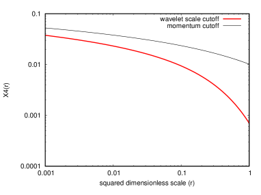
Figure 1: Plot of the one-loop contribution to the $\phi^{4}$ vertex, calculated with the first derivative of the Gaussian as the mother wavelet as a function of the squared observation scale $r=A^{2}s^{2}$, compared to that calculated with the standard cutoff at the cutoff momentum $\Lambda=A^{-1}$ in Euclidean $d=4$ dimensions.

The slopes of both curves in UV limit ($A\to 0$) are the same: $\frac{\partial\lambda}{\partial\mu}=\frac{3\lambda^{2}}{16\pi^{2}}$.

The running coupling constant $\lambda(\alpha^{2})$ can be understood as the coupling that folds into its running all quantum effects characterized by a scale larger than the observation scale $A$.

For small $\alpha$, Eq.(26) tends to the known result. This is because we have started with the local Ginzburg-Landau theory, where the fluctuations of all scales interact with each other, with the interaction of neighbouring scales being most important; see, e.g.Wilson and Kogut (1974) for an excellent discussion of the underlying physics.

III.4 QED: wavelet regularization of a local gauge theory

Quantum electrodynamics is the simplest gauge theory of the type given in Eq. (4), with the gauge group being the Abelian group $U(1)$:

$$\psi(x)\to e^{-\imath e\Lambda(x)}\psi(x).$$ (28)

The transformation of the gauge field – the electromagnetic field – is the gradient transformation:

$$A_{\mu}(x)\to A_{\mu}(x)+\partial_{\mu}\Lambda(x).$$ (29)

In view of the linearity of the wavelet transform, Eq. (29) keeps the same form for all scale components of the gauge field $A_{\mu,a}(x)$ – in contrast to the matter field transformation [Eq.(28)], which is nonlinear – and thus, the gauge transform of the matter fields in a local gauge theory is not the change of all scale components $\psi_{a}(x)$ by the same phase.

The Euclidean QED Langangian is:

$$L = \bar{\psi}(x)(\not{D}+\imath m)\psi(x)+\frac{1}{4}F_{\mu\nu}F_{\mu\nu}+\underbrace{\frac{1}{2\alpha}(\partial_{\mu}A_{\mu})^{2}}_{\hbox{gauge fixing}},$$ (30)

$$D_{\mu}\equiv\partial_{\mu}+\imath eA_{\mu}(x),\hbox{with\ }F_{\mu\nu}=\partial_{\mu}A_{\nu}-\partial_{\nu}A_{\mu}$$

which is the field strength tensor of the electromagnetic field $A_{\mu}(x)$. (The slashed vectors denote the convolution with the Dirac $\gamma$ matrices: $\not{D}\equiv\gamma_{\mu}D_{\mu}$.)

The wavelet regularization technique works for QED in the same way as it does for the above considered scalar field theory. This means that each line of the Feynman diagram carrying momentum $p$ acquires a cutoff factor $f^{2}(Ap)$.

In this way, in one-loop approximation, we get the electron self-energy, shown in Fig. 2:

[small,horizontal= a to b] i1[particle=a] – [fermion,momentum=$p$] a – [photon, half left,momentum=$q+p/2$] b –[fermion,momentum=$p$] o1[particle=a’], a – [fermion] b ;

Figure 2: Electron self-energy diagram in scale-dependent QED .

$$\frac{\Sigma^{(A)}(p)}{\tilde{\chi}(ap)\tilde{\chi}(-a^{\prime}p)}=-\imath e^{2}\int\frac{d^{4}{q}}{(2\pi)^{4}}\frac{F_{A}(p,q)\gamma_{\mu}\left[\frac{\not{p}}{2}-\not{q}-m\right]\gamma_{\mu}}{\left[\left(\frac{p}{2}-q\right)^{2}+m^{2}\right]\left[\frac{p}{2}+q\right]^{2}},$$ (31)

where

$$F_{A}(p,q)\equiv f^{2}\left(A(\frac{p}{2}+q)\right)f^{2}\left(A(\frac{p}{2}-q)\right)=e^{-A^{2}p^{2}-4A^{2}q^{2}}$$

is the product of the wavelet cutoff factors, and $A=\min(a,a^{\prime})$ is the minimal scale of two external lines of the diagram Fig. 2.

Similarly, for the vacuum polarization diagram of QED, shown in Fig. 3, we get Altaisky (2007)

$$\frac{\Pi_{\mu\nu}^{(A)}(p)}{\tilde{\chi}(ap)\tilde{\chi}(-a^{\prime}p)} = -e^{2}\int\frac{d^{4}{q}}{(2\pi)^{4}}F_{A}(p,q)\times$$

$$\times \frac{\mathrm{Tr}(\gamma_{\mu}(\not{q}+\not{p}/2-m)\gamma_{\nu}(\not{q}-\not{p}/2-m))}{\left[(q+p/2)^{2}+m^{2}\right]\left[(q-p/2)^{2}+m^{2}\right]}.$$ (32)

[small,horizontal= a to b] i1[particle=a] – [photon,momentum=$p$] a – [fermion, half left,momentum=$q+p/2$] b –[photon,momentum=$p$] o1[particle=a’], b – [fermion,half left] a ;

Figure 3: Vacuum polarization diagram in scale-dependent QED .

The electron-photon interaction vertex, in one-loop approximation, with the photon propagator taken in the Feynman gauge, gives the equation

$$\frac{\Gamma_{\mu,r}^{(A)}}{\tilde{\chi}(-pa^{\prime})\tilde{\chi}(-qr)\tilde{\chi}(ka)}=e^{2}\int\frac{d^{4}{f}}{(2\pi)^{4}}\gamma_{\alpha}\frac{\not{p}-\not{f}-m}{(p-f)^{2}+m^{2}}$$

$$\times\gamma_{\mu}\frac{\not{k}-\not{f}-m}{(k-f)^{2}+m^{2}}\gamma_{\alpha}\frac{1}{f^{2}}f^{2}(A(p-f))f^{2}(A(k-f))f^{2}(Af).$$ (33)

The vertex function [Eq.(33)] and the inverse propagator are related by the Ward-Takahashi identities, which are wavelet transforms of corresponding identities of the ordinary local gauge theory (Albeverio and Altaisky, 2011; Altaisky and Kaputkina, 2013a). The detailed one-loop calculations, except for the contribution to the vertex, can be found in Ref.Altaisky and Kaputkina (2013a). As for the vertex contribution [Eq.(33)], shown in Fig. 4, the calculation is rather cumbersome, but it can be done numerically.

Figure 4: One-loop vertex function in scale-dependent QED

IV Gauge invariance for scale-dependent fields

For a non-Abelian gauge theory both terms in the gauge field transformation [Eq.(5)] are nonlinear. The wavelet transform [Eq.(18)] can hardly be applied to the theory without violation of local gauge invariance. An attempt to use wavelets for gauge theories, QED and QCD, was undertaken for the first time by P.Federbush Federbush (1995) in a form of discrete wavelet transform. Later, it was extended by using the wavelet transform in lattice simulations and theoretical studies of related problems Halliday and Suranyi (1995); Battle (1999); Michlin et al. (2017). The consideration was restricted to axial gauge and a special type of divergency-free wavelets in four dimensions. The context of that application was the localization of the wavelet basis, which may be beneficial for numerical simulation, but is not tailored for analytical studies, and does not link the gauge invariance to the dependence on scale. The discrete wavelet transform approach to different quantum field theory problems has been further developed in Hamiltonian formalism, but for scalar theories with local interaction Brennen et al. (2015); Michlin et al. (2017).

Now it is a point to think of how we can build a gauge-invariant theory of fields that depend on both the position ($x$) and the resolution ($a$). To do this, we recall that the free fermion action [Eq.(1)] can be considered as a matrix element of the Dirac operator:

$$S_{E}=\langle\psi|\gamma_{\mu}\partial_{\mu}+\imath m|\psi\rangle.$$ (34)

Assuming a scalar product $\langle\cdot|\cdot\rangle$ in a general Hilbert space $\mathcal{H}$, in accordance with the original Dirac’s formulation of quantum field theory Dirac (1958), we can insert arbitrary partitions of unity $\hat{1}=\sum_{c}|c\rangle\langle c|$ into Eq. (34), so that

$$S_{E}=\sum_{c,c^{\prime}}\langle\psi|c\rangle\langle c|\gamma_{\mu}\partial_{\mu}+\imath m|c^{\prime}\rangle\langle c^{\prime}|\psi\rangle.$$

An important type of the unity partition in Hilbert space $\mathcal{H}$ is a unity partition related to the generalized wavelet transform [Eq.(8)]:

$$\hat{1}=\int_{G}\Omega(\nu)|\chi\rangle\frac{d\mu_{L}(\nu)}{C_{\chi}}\langle\chi|\Omega^{\dagger}(\nu).$$ (35)

Our main criterion for this choice is to find a group $G$ which pertains to the physics of quantum measurement and provides the fields defined on finite domains rather than points. The group that can leverage this task is a group of affine transformations:

$$G:x^{\prime}=ax+b,a\in\mathbb{R}_{+},x^{\prime},x,b\in\mathbb{R}^{d}.$$ (36)

Following Refs.Altaisky (2010); Altaisky and Kaputkina (2013a), we consider an isotropic theory. The representation of the affine group [Eq.(36)] in $L^{2}(\mathbb{R}^{d})$ is chosen as

$$[\Omega(a,b)\chi](x):=\frac{1}{a^{d}}\chi\left(\frac{x-b}{a}\right),$$ (37)

and the left-invariant Haar measure is

$$d\mu_{L}(a,b)=\frac{dad^{d}b}{a}.$$ (38)

In view of the linearity of the wavelet transform

$$\psi(x)\to\psi_{a}(b)=\int_{\mathbb{R}^{d}}\frac{1}{a^{d}}\bar{\chi}\left(\frac{x-b}{a}\right)\psi(x)d^{d}x,$$ (39)

the action on the affine group [Eq.(36)] keeps the same form as the action of the genuine theory [Eq.(34)]. Thus, we get the action functional for the fields $\psi_{a}(b)$ defined on the affine group:

$$S_{E} = \frac{1}{C_{\chi}}\int_{\mathbb{R}_{+}\otimes\mathbb{R}^{d}}\Bigl{[}\bar{\psi}_{a}(b)\gamma_{\mu}\partial_{\mu}\psi_{a}(b)$$

$$+ \imath m\bar{\psi}_{a}(b)\psi_{a}(b)\Bigr{]}\frac{dad^{d}b}{a},$$ (40)

where the derivatives $\partial_{\mu}$ are now taken with respect to spatial variables $b_{\mu}$. The meaning of the representation Eq.(40) is that the action functional is now a sum of independent scale components $S_{E}=\int S(a)\frac{da}{a}$, with no interaction between the scales.

Starting from the locally gauge invariant action $S_{E}=\int d^{4}x\bar{\psi}(\not{D}+\imath m)\psi$ we destroy such independence by the cubic term $\bar{\psi}\not{A}\psi$, which yields cross-scale terms. However, knowing nothing about the point-dependent gauge fields $A_{\mu}(x)$ at this stage, we should certainly ask the question of how one can make the theory of Eq.(40) invariant with respect to a phase transformation defined locally on the affine group:

$$U_{a}(b)=\exp\left(\imath\sum_{A}w^{A}_{a}(b)T^{A}\right)?$$ (41)

Since the action [Eq.(40)], for each fixed value of the scale $a$, has exactly the same form as the standard action [Eq.(1)], we can introduce the invariance with respect to local phase transformation separately at each scale by changing the derivative $\partial_{\mu}\equiv\frac{\partial}{\partial b_{\mu}}$ into the covariant derivative

$$D_{\mu,a}=\partial_{\mu}+\imath A_{\mu,a}(b),$$ (42)

with the gauge transformation law for the scale-dependent gauge field $A_{\mu,a}(b)=\sum_{A}A_{\mu,a}^{A}(b)T^{A}$ identical to Eq.(5):

$$A_{\mu,a}^{\prime}(b)=U_{a}(b)A_{\mu,a}(b)U^{\dagger}_{a}(b)+\imath\left(\partial_{\mu}U_{a}(b)\right)U^{\dagger}_{a}(b).$$

Similarly, for the field strength tensor and for the Yang-Mills Lagrangian:

$$F_{\mu\nu,a}=-\imath[D_{\mu,a},D_{\nu,a}],\ L_{a}^{YM}=\frac{1}{2g^{2}}\mathrm{Tr}(F_{\mu\nu,a}F_{\mu\nu,a}).$$ (43)

Assuming the formal coupling constant of the gauge field $A_{\mu,a}(b)$ to be dependent on scale only, we can rewrite the covariant derivative by changing $A_{\mu,a}(b)$ to $g(a)A_{\mu,a}(b)$:

$$D_{\mu,a}=\partial_{\mu}+\imath gA_{\mu,a}(b).$$ (44)

This means we have a collection of identical gauge theories for the fields $\psi_{a}(b),A_{\mu,a}(b)$, labeled by the scale variable $a$, which differ from each other only by the value of the scale-dependent coupling constant $g=g(a)$. It is a matter of choice whether to keep the scale dependence in $g(a)$, or solely in $A_{\mu,a}(b)$. The Euclidean action of the multiscale theory takes the form

$$S_{E} = \frac{1}{C_{\chi}}\int\frac{dad^{d}b}{a}\Bigl{[}\bar{\psi}_{a}(b)(\gamma_{\mu}D_{\mu,a}+\imath m)\psi_{a}(b)+$$

$$+ \frac{1}{4}F_{\mu\nu,a}^{A}F_{\mu\nu,a}^{A}\Bigr{]}+\hbox{gauge fixing terms},$$ (45)

where

$$F_{\mu\nu,a}^{A}=\partial_{\mu}A^{A}_{\nu,a}-\partial_{\nu}A^{A}_{\mu,a}-gf^{ABC}A^{B}_{\mu,a}A^{C}_{\nu,a}.$$

The difference between the standard quantum field theory formalism and the field theory with action (45), defined on the affine group, consists in changing the integration measure from $d^{d}x$ to the left-invariant measure on the affine group [Eq.(38)]. So, the generating functional can be written in the form

$$Z[J_{a}(b)]=\int\mathcal{D}\Phi_{a}(b)e^{-S_{E}[\Phi]+\int\frac{dad^{4}b}{C_{\chi}a}\Phi_{a}(b)J_{a}(b)},$$ (46)

where $\Phi_{a}(b)=(A_{a,\mu}(b),\psi_{a}(b),\ldots)$ is the full set of all scale-dependent fields present in the theory. Since the ”Lagrangian” in the action (45), for each fixed value of $a$, has exactly the same form as that in standard theory, the Faddeev-Popov gauge-fixing procedure Faddeev and Popov (1967) can be introduced to the scale-dependent theory in a straightforward way.

IV.1 Feynman diagrams

The same as in wavelet-regularization of a local theory, described in Sec. III, here we understand the physically observed fields as the sums of scale components from the observation scale $A$ to infinity Altaisky (2010):

$$\psi^{A}(x)=\frac{1}{C_{\chi}}\int_{A}^{\infty}\frac{da}{a}\int d^{d}b\frac{1}{a^{d}}\chi\left(\frac{x-b}{a}\right)\psi_{a}(b).$$

The free-field Green functions at a given scale $a$ are projections of the ordinary Green function to the scale $a$ performed by the $\chi$ wavelet filters:

$$G_{a_{1},\ldots,a_{n}}(k_{1},\ldots,k_{n})=\tilde{\bar{\chi}}(a_{1}k_{1})\ldots\tilde{\bar{\chi}}(a_{n}k_{n})G(k_{1},\ldots,k_{n}).$$

The interacting-field Green functions, according to the action [Eq.(45)], can be constructed if we provide the equality of all scale arguments by ascribing the multiplier $g(a)\prod_{i}\delta(\ln a_{i}-\ln a)$ to each vertex, and $\delta(\ln a_{i}-\ln a_{j})$ to each line of the Feynman diagram. This is different from the local theory, described in Sec. III, where all scale components do interact with each other. Now we do not yield the cutoff factor $f^{2}(\cdot)$ on each internal line, with $f(x)$ given by the scale integration (20). Instead, we have to put the wavelet filter modulus squared on each internal line. This suppresses not only the UV divergences, but also the IR divergences. As a result, we arrive at the following diagram technique, which is (up to the above mentioned cutoff factors), identical to standard Feynman rules for Yang-Mills theory; see, e.g., Ref. Ramond (1989).

The propagator for the spin-half fermions:

$$\feynmandiagram[horizontal=ctod]{c[particle=c]--[fermion,edgelabel=p]d[particle=d],};=\imath\delta_{cd}\frac{\not{p}-m}{p^{2}+m^{2}}|\tilde{\chi}(ap)|^{2},$$

where $c,d$ are the indices of the fermion representation of the gauge group.

The propagator of the gauge field (taken in the Feynman gauge):

$$\feynmandiagram[horizontal=AtoB]{A[particle=A]--[boson,momentum=p]B[particle=B],};=\delta_{AB}\frac{1}{p^{2}}\delta_{\mu\nu}|\tilde{\chi}(ap)|^{2}$$

The gluon to fermion coupling:

$$\leavevmode\hbox to0pt{\vbox to0pt{\text{[drawing]}}}=-\imath g(a)\gamma_{\mu}(T^{A})_{cd} c d A c d A$$

The three-gluon vertex:

$$\leavevmode\hbox to0pt{\vbox to0pt{\text{[drawing]}}}=-\imath g(a)f^{ABC}\bigl{[}(r_{\mu}-q_{\mu})\delta_{\nu,\rho}+ B,\nu A,\mu C,\rho$$

$$+(q_{\rho}-p_{\rho})\delta_{\mu\nu}+(p_{\nu}-r_{\nu})\delta_{\rho\mu}\bigr{]}$$ (47)

All momenta are incident to the vertex: $p+q+r=0$.

Similarly, for the four-gluon vertex:

$$\leavevmode\hbox to0pt{\vbox to0pt{\text{[drawing]}}}=-g^{2}(a)\Bigl{[}f^{ABE}f^{CDE}(\delta_{\mu\rho}\delta_{\nu\sigma}-\delta_{\nu\rho}\delta_{\mu\sigma})+f^{CBE}f^{ADE}(\delta_{\mu\rho}\delta_{\nu\sigma}-\delta_{\nu\mu}\delta_{\rho\sigma}) A,\mu B,\nu C,\rho D,\sigma$$

$$+f^{DBE}f^{CAE}(\delta_{\sigma\rho}\delta_{\nu\mu}-\delta_{\nu\rho}\delta_{\mu\sigma})\Bigr{]}.$$

The ghost propagator:

$$\feynmandiagram[nodes=circle,small,horizontal=AtoB]{A--[scalar,momentum=p]B,};=-\imath\frac{\delta^{AB}}{p^{2}}|\tilde{\chi}(ap)|^{2}.$$

The gluon-to-ghost interaction vertex:

$$\leavevmode\hbox to0pt{\vbox to0pt{\text{[drawing]}}}=\frac{1}{2}g(a)f^{ABC}(r_{\mu}+p_{\mu}-q_{\mu})=-g(a)f^{ABC}q_{\mu}, A B C,\mu A B C,\mu$$

with $r+p+q=0$.

For simplicity, in the following calculations I use the first derivative of Gaussian as a mother wavelet [Eq.(21)], which provides the cancellation of both the UV and the IR divergences by virtue of $|\tilde{\chi}(\cdot)|^{2}$ on each propagator line. For the chosen wavelet [Eq. (21)], the wavelet cutoff factor is

$$F_{a}(p)=(ap)^{2}e^{-a^{2}p^{2}}$$ (48)

for each line of the diagram, calculated for the scale $a$ of the considered model.

IV.2 Scale dependence of the gauge coupling constant

To study the scale dependence of the gauge coupling constant we can start with a pure gauge field theory without fermions, along the lines of Ref.Gross and Wilczek (1973). The total one-loop contribution to three gluon interaction is given by the diagram equation (49):

$$\leavevmode\hbox to0pt{\vbox to0pt{\text{[drawing]}}}=\leavevmode\hbox to0pt{\vbox to0pt{\text{[drawing]}}}+\leavevmode\hbox to0pt{\vbox to0pt{\text{[drawing]}}}+\frac{1}{2}\Bigl{[}\leavevmode\hbox to0pt{\vbox to0pt{\text{[drawing]}}}+\hbox{permutations}\Bigr{]}+\hbox{ghost loops} C B A C B A C B A C B A A B C B A C B A C B A C B A A B$$ (49)

In standard QCD, theory the one-loop contribution to the three-gluon vertex is calculated in the Feynman gauge Ball and Chiu (1980). This was later generalized to an arbitrary covariant gauge Davydychev et al. (1996). These known results, being general in kinematic structure, are based on dimensional regularization, and thus are determined by the divergent parts of integrals. Different corrections to the perturbation expansion based on analyticity have been proposed Shirkov and Solovtsov (2007); Bakulev et al. (2010), but they are still based on divergent graphs. In this context, QCD is often considered as an effective theory, which describes the low-energy limit for a set of asymptotically observed fields, obtained by integrating out all heavy particles Georgi (1993). The effective theory is believed to be derivable from a future unified theory, which includes gravity.

The essential artifact of renormalized QCD is the logarithmic decay of the running coupling constant $\alpha_{s}(Q^{2})$ at infinite momentum transfer $Q^{2}\,\to\,\infty$, known as asymptotic freedom. With the help of $\overline{MS}$, the calculations are available up to the five-loop approximation Baikov et al. (2017).

In the present paper, I do not pretend to derive the logarithmic law. Instead, I have shown, that if our understanding of gauge invariance is true in an arbitrary functional basis, based on a Lie group representation, we use to measure physical fields, the resulting theory is finite by construction. The restriction of calculations to the Feynman gauge and the specific form of the mother wavelet are technical simplifications, with which we proceed to make the results viewable.

The first term on the rhs of Eq.(49) is the unrenormalized three-gluon vertex [Eq.(47)]. The second graph is the gluon loop shown in Fig. 5:

Figure 5: Gluon loop contribution to the three-gluon vertex; $p_{1}+p_{2}+p_{3}=0$.

Its value is

$$\Gamma^{ABC}_{\mu_{1}\mu_{2}\mu_{3}}=-\imath g^{3}(a)\frac{C_{A}}{2}f^{ABC}V_{\mu_{1},\mu_{2},\mu_{3}}^{\mathrm{one-loop}}(p_{1},p_{2},p_{3}),$$ (50)

where the common color factor is $C_{A}=2T_{F}N_{C}$, $N_{C}$ is the number of colors, and $T_{F}=\frac{1}{2}$ is the usual normalization of generators in fundamental representation; see, e.g., Ref.Grozin (2007).

IV.2.1 Gluon loop contribution

We calculate the one-loop tensor structure $V_{\mu_{1},\mu_{2},\mu_{3}}^{\mathrm{one-loop}}(p_{1},p_{2},p_{3})$ in the Feynman gauge. After symmetrization of the loop momenta in diagram (50),

$$l_{1}=f+\frac{p_{3}-p_{2}}{3},l_{2}=f+\frac{p_{1}-p_{3}}{3},l_{3}=f+\frac{p_{2}-p_{1}}{3},$$

the tensor structure of the diagram takes the form

$$V_{\mu_{1},\mu_{2},\mu_{3}}^{\mathrm{one-loop}}(p_{1},p_{2},p_{3},f)=V_{\mu_{1},\alpha,\beta}(p_{1},l_{3},-l_{2})$$

$$\times V_{\alpha,\mu_{2},\delta}(-l_{3},p_{2},l_{1})V_{\delta,\mu_{3},\beta}(-l_{1},p_{3},l_{2}),$$ (51)

where

$$V_{\mu_{1},\mu_{2},\mu_{3}}(p_{1},p_{2},p_{3}):=(p_{3,\mu_{1}}-p_{2,\mu_{1}})\delta_{\mu_{2},\mu_{3}}+$$

$$+(p_{1,\mu_{2}}-p_{3,\mu_{2}})\delta_{\mu_{3},\mu_{1}}+(p_{2,\mu_{3}}-p_{1,\mu_{3}})\delta_{\mu_{1},\mu_{2}}$$ (52)

is the tensor structure of the three-gluon interaction vertex [Eq.(47)].

The tensor structure of Eq. (50) can be represented as a sum of two terms: the first term is free of loop momentum $f$, and the second term is quadratic in it:

$$V_{\mu_{1},\mu_{2},\mu_{3}}^{\mathrm{one-loop}}(p_{1},p_{2},p_{3},f)=V^{0}(p_{1},p_{2},p_{3})+V^{1}(p_{1},p_{2},p_{3},f)$$

with

$$V^{1}_{\mu_{1},\mu_{2},\mu_{3}}(p_{1},p_{2},p_{3},f)=3\bigl{[}f_{\mu_{1}}f_{\mu_{3}}(p_{1,\mu_{2}}-p_{3,\mu_{2}})+$$

$$+f_{\mu_{1}}f_{\mu_{2}}(p_{2,\mu_{3}}-p_{1,\mu_{3}})+f_{\mu_{2}}f_{\mu_{3}}(p_{3,\mu_{1}}-p_{2,\mu_{1}})\bigr{]}+$$

$$+\frac{7}{3}f^{2}\bigl{[}(p_{3,\mu_{1}}-p_{2,\mu_{1}})\delta_{\mu_{2},\mu_{3}}+(p_{1,\mu_{2}}-p_{3,\mu_{2}})\delta_{\mu_{3},\mu_{1}}+$$

$$+(p_{2,\mu_{3}}-p_{1,\mu_{3}})\delta_{\mu_{1},\mu_{2}}\bigr{]}+\frac{2}{3}\bigl{[}\delta_{\mu_{1}\mu_{2}}f_{\mu_{3}}f_{\alpha}(p_{2,\alpha}-p_{1,\alpha})+$$

$$\delta_{\mu_{1}\mu_{3}}f_{\mu_{2}}f_{\alpha}(p_{1,\alpha}-p_{3,\alpha})+\delta_{\mu_{2}\mu_{3}}f_{\mu_{1}}f_{\alpha}(p_{3,\alpha}-p_{2,\alpha})\bigr{]}$$

Integrating the equation $V^{1}_{\mu_{1},\mu_{2},\mu_{3}}(p_{1},p_{2},p_{3},f)$ with the Gaussian weight we substitute $f_{\mu}f_{\nu}\to\frac{\delta_{\mu\nu}}{d}f^{2}$ into the Gaussian integral $\int e^{-\zeta f^{2}}f^{2}d^{d}f=\frac{d}{2}\pi^{\frac{d}{2}}\zeta^{-\frac{d}{2}-1}$. With $\zeta=3a^{2},d=4$, this gives the tensor structure

$$V^{1}(p_{1},p_{2},p_{3})=\frac{13}{864\pi^{2}}e^{-\frac{2}{9}a^{2}[p_{1}^{2}+p_{2}^{2}+p_{3}^{2}-p_{1}p_{2}-p_{1}p_{3}-p_{2}p_{3}]}$$

$$\times V_{\mu_{1},\mu_{2},\mu_{3}}(p_{1},p_{2},p_{3}).$$

The part of the tensor structure that does not contain $f$ contributes a term proportional to the Gaussian integral $\int e^{-\zeta f^{2}}d^{d}f=\left(\frac{\pi}{\zeta}\right)^{\frac{d}{2}}$. This gives

$$\frac{a^{2}}{144\pi^{2}}e^{-\frac{2}{3}a^{2}[p_{1}^{2}+p_{2}^{2}+p_{1}p_{2}]}V^{0}_{\mu_{1},\mu_{2},\mu_{3}}(p_{1},p_{2},p_{3}=-p_{1}-p_{2})$$

where

$$V^{0}_{\mu_{1},\mu_{2},\mu_{3}}(p_{1},p_{2})=\frac{4}{3}(p_{2,\mu_{1}}p_{2,\mu_{2}}p_{2,\mu_{3}}-p_{1,\mu_{1}}p_{1,\mu_{2}}p_{1,\mu_{3}})$$

$$+\frac{5}{3}(p_{2,\mu_{1}}p_{2,\mu_{2}}p_{1,\mu_{3}}-p_{1,\mu_{1}}p_{1,\mu_{2}}p_{2,\mu_{3}})$$

$$+\frac{2}{3}(p_{2,\mu_{2}}p_{2,\mu_{3}}p_{1,\mu_{1}}-p_{1,\mu_{1}}p_{1,\mu_{3}}p_{2,\mu_{2}})$$

$$+\frac{1}{3}(p_{1,\mu_{2}}p_{1,\mu_{3}}p_{2,\mu_{1}}-p_{2,\mu_{1}}p_{2,\mu_{3}}p_{1,\mu_{2}})$$

$$+\frac{37}{27}\delta_{\mu_{1}\mu_{2}}p_{1}p_{2}(p_{2,\mu_{3}}-p_{1,\mu_{3}})+\frac{58}{27}\delta_{\mu_{1}\mu_{2}}(p_{1}^{2}p_{2,\mu_{3}}-p_{2}^{2}p_{1,\mu_{3}})$$

$$+\frac{5}{27}(\delta_{\mu_{2}\mu_{3}}p_{1}^{2}p_{1,\mu_{1}})-\delta_{\mu_{1}\mu_{3}}p_{2}^{2}p_{2,\mu_{2}}-\delta_{\mu_{1}\mu_{2}}p_{2}^{2}p_{2,\mu_{3}})$$

$$+\frac{32}{27}(\delta_{\mu_{1}\mu_{3}}p_{1,\mu_{2}}(p_{1}^{2}+p_{1}p_{2})-\delta_{\mu_{2}\mu_{3}}p_{2,\mu_{1}}(p_{2}^{2}+p_{1}p_{2}))$$

$$+\frac{16}{27}(\delta_{\mu_{1}\mu_{3}}p_{1}^{2}p_{2,\mu_{2}}-\delta_{\mu_{2}\mu_{3}}p_{2}^{2}p_{1,\mu_{1}})$$

$$+\frac{53}{27}(\delta_{\mu_{1}\mu_{3}}p_{2}^{2}p_{1,\mu_{2}}-\delta_{\mu_{2}\mu_{3}}p_{1}^{2}p_{2,\mu_{1}})$$

$$+\frac{47}{27}p_{1}p_{2}(\delta_{\mu_{2}\mu_{3}}p_{1,\mu_{1}}-\delta_{\mu_{1}\mu_{3}}p_{2,\mu_{2}})$$

Summing these two terms, we get

$$\Gamma_{\mu_{1}\mu_{2}\mu_{3}}^{ABC}(p_{1},p_{2})=-\imath g^{3}(a)\frac{C_{A}}{2}\frac{f^{ABC}}{144\pi^{2}}\times$$

$$\times e^{-\frac{2}{3}a^{2}(p_{1}^{2}+p_{2}^{2}+p_{1}p_{2})}\Bigl{[}a^{2}V^{0}_{\mu_{1}\mu_{2}\mu_{3}}(p_{1},p_{2})+$$ (53)

$$+\frac{13}{6}V_{\mu_{1}\mu_{2}\mu_{3}}(p_{1},p_{2},-p_{1}-p_{2})\Bigr{]},$$

where $V_{\mu_{1}\mu_{2}\mu_{3}}$, given by Eq.(52), is the tensor structure of the unrenormalized three-gluon vertex.

IV.2.2 Contribution of four-gluon vertex

The next one-loop contribution to the three-gluon vertex comes from the diagrams with four-gluon interaction, of the type shown in Fig. 6.

Figure 6: One-loop contribution to the three-gluon vertex provided by four-gluon interaction.

In the case of four-gluon contribution the common color factor cannot be factorized: instead there are three similar diagrams with gluon loops inserted in each gluon leg: $p_{3}$, $p_{2}$ and $p_{1}$, respectively. The case of $p_{3}$ is shawn in Fig. 6.

The one-loop contribution to a three-gluon vertex shown in Fig. 6 can be easily calculated taking into account that the squared momenta in gluon propagators are cancelled by wavelet factors [Eq.(48)]. This gives

$$a^{4}\int(-\imath g(a))f^{DEC}\bigl{[}(2p_{3}-f)_{\delta}\delta_{\mu_{3}\epsilon}+(-f-p_{3})_{\epsilon}\delta_{\mu_{3}\delta}+$$

$$+(2f-p_{3})_{\mu_{3}}\delta_{\epsilon\delta}\bigr{]}\times$$

$$\times(-g(a))^{2}\bigl{[}f^{AEX}f^{BDX}(\delta_{\mu_{1}\mu_{2}}\delta_{\epsilon\delta}-\delta_{\epsilon\mu_{2}}\delta_{\mu_{1}\delta})+$$

$$+f^{BEX}f^{ADX}(\delta_{\mu_{1}\mu_{2}}\delta_{\epsilon\delta}-\delta_{\epsilon\mu_{1}}\delta_{\mu_{2}\delta})+$$

$$+f^{DEX}f^{BAX}(\delta_{\delta\mu_{2}}\delta_{\epsilon\mu_{1}}-\delta_{\epsilon\mu_{2}}\delta_{\mu_{1}\delta})\bigr{]}\times$$

$$\times\exp\bigl{(}-a^{2}f^{2}-a^{2}(f+p_{1}+p_{2})^{2}\bigr{)}\frac{d^{4}f}{(2\pi)^{4}}.$$

The presence of four-gluon interaction does not allow for the factorization of the common color factor. Instead, there are three different terms in color space:

$$f^{DEC}f^{AEX}f^{BDX}=-\frac{C_{A}}{2}f^{ABC},$$

$$f^{DEC}f^{BEX}f^{ADX}=+\frac{C_{A}}{2}f^{ABC},$$ (54)

$$f^{DEC}f^{DEX}f^{BAX}=-C_{A}f^{ABC}$$

with the normalization condition

$$f^{ACD}f^{BCD}=C_{A}\delta_{AB}.$$

There are two Gaussian integrals contributing to the diagram shown in Fig. 6:

$$I(s) = \int\frac{d^{4}f}{(2\pi)^{4}}e^{-2a^{2}f^{2}-2a^{2}sf}=\frac{1}{64\pi^{2}a^{4}}e^{\frac{a^{2}s^{2}}{2}},$$

$$I_{\mu}(s) = \int\frac{d^{4}f}{(2\pi)^{4}}f_{\mu}e^{-2a^{2}f^{2}-2a^{2}sf}=-\frac{s_{\mu}}{128\pi^{2}a^{4}}e^{\frac{a^{2}s^{2}}{2}},$$

where $s=p_{1}+p_{2}$.

Thus we can express the tensor coefficients at the three terms in Eq.(54) as

$$T_{1} = -\frac{3}{2}\delta_{\mu_{1}\mu_{3}}s_{\mu_{2}}+\frac{3}{2}\delta_{\mu_{2}\mu_{3}}s_{\mu_{1}},$$

$$T_{2} = +\frac{3}{2}\delta_{\mu_{1}\mu_{3}}s_{\mu_{2}}-\frac{3}{2}\delta_{\mu_{2}\mu_{3}}s_{\mu_{1}},$$ (55)

$$T_{3} = 3(\delta_{\mu_{2}\mu_{3}}s_{\mu_{1}}-\delta_{\mu_{1}\mu_{3}}s_{\mu_{2}}),$$

respectively. The sum of all three terms $-\frac{C_{A}}{2}f^{ABC}T_{1}+\frac{C_{A}}{2}f^{ABC}T_{2}-C_{A}f^{ABC}T_{3}$ gives

$$\frac{9}{2}C_{A}f^{ABC}[\delta_{\mu_{1}\mu_{3}}s_{2}-\delta_{\mu_{2}\mu_{3}}s_{\mu_{1}}],$$

and thus the whole integral

$$V_{\mu_{1}\mu_{2}\mu_{3}}^{ABC}(s)=\frac{\imath g^{3}(a)}{64\pi^{2}}e^{\frac{-a^{2}s^{2}}{2}}\frac{9C_{A}}{2}f^{ABC}[\delta_{\mu_{1}\mu_{3}}s_{\mu_{2}}-\delta_{\mu_{2}\mu_{3}}s_{\mu_{1}}].$$ (56)

Two more contributing diagrams, symmetric to Fig. 6, are different from the above calculated $V(A,\mu_{1},p_{1};B,\mu_{2},p_{2};C,\mu_{3},p_{3})$ only by changing $B,\mu_{2},p_{2}\leftrightarrow C,\mu_{3},p_{3}$ and $A,\mu_{1},p_{1}\leftrightarrow C,\mu_{3},p_{3}$, respectively. This gives two more terms

$$V_{\mu_{1}\mu_{2}\mu_{3}}^{ABC}(t)=\frac{\imath g^{3}(a)}{64\pi^{2}}e^{\frac{-a^{2}t^{2}}{2}}\frac{9C_{A}}{2}f^{ACB}[\delta_{\mu_{1}\mu_{2}}t_{\mu_{3}}-\delta_{\mu_{2}\mu_{3}}t_{\mu_{1}}],$$

$$V_{\mu_{1}\mu_{2}\mu_{3}}^{ABC}(u)=\frac{\imath g^{3}(a)}{64\pi^{2}}e^{\frac{-a^{2}u^{2}}{2}}\frac{9C_{A}}{2}f^{CBA}[\delta_{\mu_{1}\mu_{3}}u_{\mu_{2}}-\delta_{\mu_{2}\mu_{1}}u_{\mu_{3}}],$$

where $t=p_{1}+p_{3}=-p_{2}$ and $u=p_{2}+p_{3}=-p_{1}$. Taking into account the common topological factor $\frac{1}{2}$ standing before all these diagrams in (49), finally we get

$$\Gamma^{ABC}_{\mu_{1}\mu_{2}\mu_{3}}(p_{1},p_{2})=\imath\frac{g^{3}(a)}{256\pi^{2}}9C_{A}f^{ABC}\Bigl{[}e^{\frac{-a^{2}s^{2}}{2}}(\delta_{\mu_{1}\mu_{3}}s_{\mu_{2}}$$

$$-\delta_{\mu_{2}\mu_{3}}s_{\mu_{1}})+e^{\frac{-a^{2}p^{2}_{2}}{2}}(\delta_{\mu_{1}\mu_{2}}p_{2,\mu_{3}}-\delta_{\mu_{2}\mu_{3}}p_{2,\mu_{1}})$$ (57)

$$+e^{\frac{-a^{2}p^{2}_{1}}{2}}(\delta_{\mu_{1}\mu_{3}}p_{1,\mu_{2}}-\delta_{\mu_{1}\mu_{2}}p_{1,\mu_{3}})\Bigr{]},$$

where $t=-p_{2},u=-p_{1},p_{3}=-p_{1}-p_{2}$.

IV.2.3 Ghost loop contribution

The last one-loop contribution not shown in Eq.(49), is the ghost loop diagram Fig. 7, and one more diagram symmetric to it.

Figure 7: Ghost loop contribution to three-gluon vertex; $p_{1}+p_{2}+p_{3}=0$.

The color factor of the diagram Fig. 7 is $f^{DEA}f^{FDB}f^{EFC}=-\frac{C_{A}}{2}f^{ABC}$. The tensor structure for diagram Fig. 7 is $l_{2,\mu_{1}}l_{3,\mu_{2}}l_{1,\mu_{3}}$, and it is $l_{3,\mu_{1}}l_{1,\mu_{2}}l_{2,\mu_{3}}$ for the symmetric diagram Grozin (2007). Ghost propagators multiplied by wavelet factors give $(-\imath)^{3}a^{6}e^{-3a^{2}f^{2}-\frac{2}{3}a^{2}(p_{1}^{2}+p_{2}^{2}+p_{1}p_{2})}$, and one more $(-1)$ accounts for the fermion loop. Finally, this gives

$$\Gamma^{ghost} = -\imath g^{3}(a)\frac{C_{A}}{2}f^{ABC}\frac{e^{-\frac{2}{3}a^{2}(p_{1}^{2}+p_{2}^{2}+p_{1}p_{2})}}{144\pi^{2}}\times$$

$$\times \bigl{[}a^{2}V_{0}+\frac{1}{18}V_{\mu_{1}\mu_{2}\mu_{3}}(p_{1},p_{2},p_{3}=-p_{1}-p_{2})\bigr{]},$$ (58)

$$V_{0} = \frac{1}{27}(p_{1,\mu_{3}}-p_{2,\mu_{3}})(p_{1,\mu_{2}}p_{2,\mu_{1}}-2p_{1,\mu_{1}}p_{2,\mu_{2}})$$

$$+ \frac{4}{27}(p_{2,\mu_{1}}p_{2,\mu_{2}}p_{2,\mu_{3}}-p_{1,\mu_{1}}p_{1,\mu_{2}}p_{1,\mu_{3}})$$

$$+ \frac{5}{27}(p_{2,\mu_{1}}p_{2,\mu_{2}}p_{1,\mu_{3}}-p_{1,\mu_{1}}p_{1,\mu_{2}}p_{2,\mu_{3}}).$$

IV.3 Study of simplified 3-gluon vertex $(p,-p,0)$

To study the scale dependence of the coupling constant let us start with a trivial situation $p_{1}=p,p_{2}=-p,p_{3}=0$. The unrenormalized vertex takes the form

$$\Gamma_{\mu_{1}\mu_{2}\mu_{3}}^{ABC}(p)=-\imath g(a)f^{ABC}V(p,-p,0),$$

where

$$V(p,-p,0)\equiv p_{\mu_{1}}\delta_{\mu_{2}\mu_{3}}+p_{\mu_{2}}\delta_{\mu_{1}\mu_{3}}-2p_{\mu_{3}}\delta_{\mu_{1}\mu_{2}}.$$

The triangle gluon loop contribution, shown in Fig. 5, is

$$\Gamma_{\mu_{1}\mu_{2}\mu_{3}}^{ABC,3}(p) = -\imath g(a)^{3}\frac{C_{A}}{2}f^{ABC}\frac{e^{-\frac{2}{3}a^{2}p^{2}}}{144\pi^{2}}\times$$

$$\times \bigl{[}a^{2}V_{0}+\frac{13}{6}V(p,-p,0)\bigr{]}$$ (59)

$$V_{0} = \frac{4}{3}p_{\mu_{1}}p_{\mu_{2}}p_{\mu_{3}}-\frac{p^{2}}{27}\bigl{(}5\delta_{\mu_{2}\mu_{3}}p_{\mu_{1}}+$$

$$+ 5\delta_{\mu_{1}\mu_{3}}p_{\mu_{2}}+32\delta_{\mu_{1}\mu_{2}}p_{\mu_{3}}\bigr{)}.$$

The contributions containing four-gluon vertexes (without fermions) give

$$\Gamma_{\mu_{1}\mu_{2}\mu_{3}}^{ABC,4}(p)=-\imath\frac{g^{3}(a)}{256\pi^{2}}9C_{A}f^{ABC}e^{-\frac{a^{2}p^{2}}{2}}V(p,-p,0).$$ (60)

The contributions of two ghost loops give

$$\Gamma^{ghost}_{\mu_{1}\mu_{2}\mu_{3}}(p,-p,0)=-\imath g^{3}(a)\frac{C_{A}}{2}\frac{f^{ABC}}{144\pi^{2}}e^{-\frac{2}{3}a^{2}p^{2}}\times$$

$$\times\frac{1}{9}\bigl{[}a^{2}\frac{4}{3}p_{\mu_{1}}p_{\mu_{2}}p_{\mu_{3}}+\frac{1}{2}V(p,-p,0)\bigr{]}.$$ (61)

Therefore, due to the use of a localized wavelet basis with a window width of size $a$, we obtain an exponential decay of the vertex function proportional to $p^{2}$.

The gauge interaction in the action functional [Eq.(45)] is not identical to that of local gauge theory (4). At this point I cannot definitely claim that physical observables are integrals of the form $\int_{A}^{\infty}\frac{da}{a}F[\phi_{a}(b)]$. If the parameter $A$ of a wavelet-regularized local theory (19) were a counterpart of a $1/\mu$ normalization scale, in our theory with scale-dependent gauge invariance the scale parameter $a$ should be treated as an independent coordinate on a $(d+1)$-dimensional group manifold ($a,\mathbf{x}$), with the scale transformations given by the generator $D=a\partial_{a}$.

Using the simplified vertex contributions [Eqs.(59)–(61)] of the one-loop scale-dependent Yang-Mills theory we can estimate the renormalization of the coupling constant $g$ in the considered theory with scale-dependent gauge invariance [Eq.(41)]. Since the scale $a$ in such a theory plays the role of the normalization scale $1/\mu$ of common models, we can calculate the $\beta$ function

$$\beta=-a^{2}\left.\frac{\partial g}{\partial a^{2}}\right|_{g_{0}=const}$$

from the equality $g_{0}=Z_{1}g$, with

$$Z_{1}=1+\frac{g^{2}C_{A}}{16\pi^{2}}\left[\frac{10}{81}e^{-\frac{2}{3}a^{2}p^{2}}+\frac{9}{16}e^{-\frac{1}{2}a^{2}p^{2}}\right]$$ (62)

calculated from the one-loop expansion (49) with the vertex contributions [Eqs.(59)–(61)]. This gives

$$\beta=-ga^{2}\frac{\partial}{\partial a^{2}}\frac{1}{Z_{1}}.$$ (63)

The equation (63) differs from standard renormalization schemes by the absence of the factor $Z_{3}^{\frac{3}{2}}$ for field renormalization. This is because each of the scale-dependent fields $A_{\mu,a}(b)$ dwells on its own scale $a$, and is not subjected to renormalization Altaisky (2016). Taking the scale derivative in Eq.(63) explicitly we get

$$\beta=-\frac{g^{3}C_{A}(ap)^{2}}{16\pi^{2}}\left[\frac{20}{243}e^{-\frac{2}{3}a^{2}p^{2}}+\frac{9}{32}e^{-\frac{1}{2}a^{2}p^{2}}\right]<0.$$ (64)

The dependence of this function on dimensionless scale $x=ap$ is shown in Fig. 8 below.

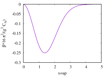
Figure 8: Dependence of the beta function [Eq.(64)] on the dimensionless scale $x=ap$. The dependence is shown in units of $\frac{g^{3}C_{A}}{16\pi^{2}}$.

The factors similar to field renormalization may be required depending on the type of observation – if we assume the observable quantity to be dependent on $\frac{\langle AAA\rangle}{\langle A\rangle^{3}}$, where the averaging $\langle\cdot\rangle$ involves integration over a certain range of scales. A more detailed study of the subject is planned for future research. Since the action In Eq.(45) comprises the fields of different scales, which do not interact to each other, to derive a phenomenological interpretation of the proposed model we need to study it within a wider framework of the Standard Model with the $SU(2)\times U(1)\times SU_{c}(3)$ gauge group to calculate the observable quantities.

V Conclusion

The basis of Fourier harmonics, an omnipresent tool of quantum field theory, is just a particular case of the decomposition of the observed field $\phi$ with respect to representations $\Omega(g)$ of the symmetry group $G$ responsible for observations. It is commonly assumed that the symmetry group of measurement is a translation group (or, more generally, the Poincaré group) the representations of which are used. We can imagine, however, that the measurement process itself is more complex, and may have symmetries more complex than the Abelian group of translations. The simplest generalization is the affine group $G:x^{\prime}=ax+b$, considered in this paper – a tool for studying scaling properties of physical systems. In this paper, I have considered the possibility to extend quantum field theory models of gauge fields, usually defined in $\mathbb{R}^{d}$ or Minkowski space, to more general space – the group of affine transformations, which includes not only translations and rotations, but also scale transformation. The peculiarity of the scale parameter ($a$) is that the scale transformation generator $D=a\partial_{a}$, in contrast to coordinate or momentum operators, is not a Hermitian operator. Hence, the scale $a$ is not a physical observable – it is a parameter of measurement – say, a scale we use in our measurements.

Following the previous papers Altaisky (2010); Altaisky and Kaputkina (2013a); Altaisky (2016), introducing explicitly a basis $\chi(a,\cdot)$ to describe quantum fields, the current paper presents a gauge theory with a gauge transformation defined separately on each scale, $\psi_{a}(x)\to e^{\imath\Omega_{a}(x)}\psi_{a}(x)$. The transformation from the usual local fields $\psi(x)$ to the scale-dependent fields, which may be referred to as the scale components of the field $\psi$ with respect to the basic function $\chi$ at a given scale $a$, is performed by means of continuous wavelet transform – a versatile tool of group representation theory. This representation is physically similar to coherent state representation Daubechies et al. (1986). The Green functions in the scale-dependent theory become finite, for both the UV and the IR divergences are suppressed by the wavelet factor $|\tilde{\chi}(ap)|^{2}$ on each internal line of the Feynman diagrams.

As a practical example of calculations, the paper presents one-loop correction to the three-gluon vertex in a pure Yang-Mills theory. The calculations are done with the mother wavelet $\chi$ being the first derivative of the Gaussian. The Green functions vanish at high momenta, which is usual for the theories with asymptotic freedom.

The existence of such a theory is merely an exciting mathematical possibility. The author does not know, which type of interaction takes place in real processes: standard local gauge theory, where all scales talk to each other due to locally defined gauge invariance, or the same-scale interaction proposed in this paper. This subject needs further investigation – at least, it seems not less elegant than the existing finite-length and noncommutative geometry models Freidel and Livine (2006); Blaschke (2010).

References

• Dyson (2007) F. Dyson, Advanced quantum mechanics (World Scientific Publishing Co., 2007).
• Stueckelberg and Petermann (1953) E. Stueckelberg and A. Petermann, Helv. Phys. Acta 26, 499 (1953).
• Bogoliuobov and Shirkov (1956) N. Bogoliuobov and D. Shirkov, Nuovo Cimento 3, 845 (1956).
• ’t Hooft and Veltman (1972) G. ’t Hooft and M. Veltman, Nuclear Physics B 44, 189 (1972).
• Altaisky (2010) M. V. Altaisky, Phys. Rev. D 81, 125003 (2010).
• Altaisky (2003) M. V. Altaisky, IOP Conf. Ser. 173, 893 (2003).
• Altaisky and Kaputkina (2013a) M. V. Altaisky and N. E. Kaputkina, Phys. Rev. D 88, 025015 (2013a).
• Goupillaud et al. (8485) P. Goupillaud, A. Grossmann,  and J. Morlet, Geoexploration 23, 85 (1984/85).
• Federbush (1995) P. Federbush, Progr. Theor. Phys. 94, 1135 (1995).
• Deur et al. (2016) A. Deur, S. Brodsky,  and G. de Téramond, Progress in Particle and Nuclear Physics 90, 1 (2016).
• Sonechkin and Datsenko (2000) D. Sonechkin and N. Datsenko, Pure and applied geophysics 157, 653 (2000).
• Altarelli (2013) G. Altarelli, PoS Corfu 2012, 002 (2013).
• Collins (1984) J. C. Collins, Renormalization (Cambridge University Press, Cambridge, England, 1984).
• Christensen and Crane (2005) J. D. Christensen and L. Crane, J. Math. Phys 46, 122502 (2005).
• Daubechies (1992) I. Daubechies, Ten lectures on wavelets (S.I.A.M., Philadelphie, 1992).
• Carey (1976) A. L. Carey, Bull. Austr. Math. Soc. 15, 1 (1976).
• Duflo and Moore (1976) M. Duflo and C. C. Moore, J. Func. Anal. 21, 209 (1976).
• Daubechies et al. (1986) I. Daubechies, G. A.,  and Y. Meyer, J. Math. Phys. 27, 1271 (1986).
• Klauder and Streater (1991) J. R. Klauder and R. F. Streater, J. Math. Phys. 32, 1609 (1991).
• Freysz et al. (1990) E. Freysz, B. Pouligny, F. Argoul,  and A. Arneodo, Phys. Rev. Lett. 64, 745 (1990).
• Altaisky (2007) M. V. Altaisky, Symmetry, Integrability and Geometry: Methods and Applications 3, 105 (2007).
• Gitman and Shelepin (2009) D. Gitman and A. Shelepin, Eur. Phys. J. C 61, 111 (2009).
• Varlamov (2012) V. Varlamov, Int.J.Theor.Phys. 51, 1453 (2012).
• Gorodnitskiy and Perel (2012) E. Gorodnitskiy and M. Perel, J. Math. Phys. 45, 385203 (2012).
• Bulut and Polyzou (2013) F. Bulut and W. Polyzou, Phys. Rev. D 87, 116011 (2013).
• Altaisky and Kaputkina (2016) M. Altaisky and N. Kaputkina, Int. J. Theor. Phys. 55, 2805 (2016).
• Altaisky and Kaputkina (2013b) M. Altaisky and N. Kaputkina, Russian Physics Journal 55, 1177 (2013b).
• Brodsky and de Téramond (2008) S. J. Brodsky and G. F. de Téramond, Phys. Rev. D 77, 056007 (2008).
• Polyzou (2020) W. Polyzou, “Wavelet representation of light-front quantum field theory,” arXiv:2002.02311 [hep-th] (2020).
• Altaisky (2016) M. V. Altaisky, Phys. Rev. D 93, 105043 (2016).
• Glimm and Jaffe (1981) J. Glimm and A. Jaffe, Quantum physics: A Functional Integral Point of View (Springer-Verlag, 1981).
• Ginzburg and Landau (1950) V. Ginzburg and L. Landau, Zh. Eksp. Teor. Fiz. 20, 1064 (1950).
• Zinn-Justin (1999) J. Zinn-Justin, Quantum field theory and critical phenomena (Oxford University Press, NY, 1999).
• Wetterich (1993) C. Wetterich, Phys. Lett. B 301, 90 (1993).
• Wilson and Kogut (1974) K. G. Wilson and J. Kogut, Physics Reports 12, 75 (1974).
• Albeverio and Altaisky (2011) S. Albeverio and M. V. Altaisky, New Advances in Physics 5, 1 (2011).
• Halliday and Suranyi (1995) I. G. Halliday and P. Suranyi, Nucl. Phys. B 436, 414 (1995).
• Battle (1999) G. Battle, Wavelets and renormalization group (World Scientific, 1999).
• Michlin et al. (2017) T. Michlin, W. N. Polyzou,  and F. Bulut, Phys. Rev. D 95, 094501 (2017).
• Brennen et al. (2015) G. K. Brennen, P. Rohde, B. C. Sanders,  and S. Singh, Phys. Rev. A 92, 032315 (2015).
• Dirac (1958) P. Dirac, The Principles of Quantum Mechanics, 4th ed. (Oxford University Press, 1958).
• Faddeev and Popov (1967) L. Faddeev and V. Popov, Phys. Lett. B 25, 29 (1967).
• Ramond (1989) P. Ramond, Field Theory: A Modern Primer, 2nd ed. (Addison-Wesley, Reading, MA, 1989).
• Gross and Wilczek (1973) D. J. Gross and F. Wilczek, Phys. Rev. D 8, 3633 (1973).
• Ball and Chiu (1980) J. Ball and T.-W. Chiu, Phys. Rev. D 22, 2550 (1980).
• Davydychev et al. (1996) A. Davydychev, P. Osland,  and O. V. Tarasov, Phys. Rev. D 54, 4087 (1996).
• Shirkov and Solovtsov (2007) D. Shirkov and I. Solovtsov, Theor. and Math. Phys. 150, 132 (2007).
• Bakulev et al. (2010) A. Bakulev, S. Mikhailov,  and N. Stefanis, JHEP 1006, 85 (2010).
• Georgi (1993) H. Georgi, Ann. Rev. Nucl. Part. Sci. 43, 209 (1993).
• Baikov et al. (2017) P. A. Baikov, K. G. Chetyrkin,  and J. H. Kühn, Phys. Rev. Lett. 118, 082002 (2017).
• Grozin (2007) A. Grozin, Lectures on QED and QCD: Practical calculation and renormalization of one- and multi-loop Feynman diagrams (World Scientific, 2007).
• Freidel and Livine (2006) L. Freidel and E. R. Livine, Phys. Rev. Lett. 96, 221301 (2006).
• Blaschke (2010) D. N. Blaschke, Euro. Phys. Lett. 91, 11001 (2010).