Receiver operating characteristic (ROC) movies, universal ROC (UROC) curves, and coefficient of predictive ability (CPA)

Abstract

Throughout science and technology, receiver operating characteristic (ROC) curves and associated area under the curve (${\rm AUC}$) measures constitute powerful tools for assessing the predictive abilities of features, markers and tests in binary classification problems. Despite its immense popularity, ROC analysis has been subject to a fundamental restriction, in that it applies to dichotomous (yes or no) outcomes only. Here we introduce ROC movies and universal ROC (UROC) curves that apply to just any linearly ordered outcome, along with an associated coefficient of predictive ability (${\rm CPA}$) measure. ${\rm CPA}$ equals the area under the UROC curve, and admits appealing interpretations in terms of probabilities and rank based covariances. For binary outcomes ${\rm CPA}$ equals ${\rm AUC}$, and for pairwise distinct outcomes ${\rm CPA}$ relates linearly to Spearman’s coefficient, in the same way that the C index relates linearly to Kendall’s coefficient. ROC movies, UROC curves, and ${\rm CPA}$ nest and generalize the tools of classical ROC analysis, and are bound to supersede them in a wealth of applications. Their usage is illustrated in data examples from biomedicine and meteorology, where rank based measures yield new insights in the WeatherBench comparison of the predictive performance of convolutional neural networks and physical-numerical models for weather prediction.
Keywords: C index; classification and regression; evaluation metric; rank correlation; coefficient; ROC analysis

1 Introduction

Originating from signal processing and psychology, popularized in the 1980s (Hanley and McNeil, 1982; Swets, 1988), and witnessing a surge of usage in machine learning (Bradley, 1997; Huang and Ling, 2005; Fawcett, 2006; Flach, 2016), receiver operating characteristic or relative operating characteristic (ROC) curves and area under the ROC curve (${\rm AUC}$) measures belong to the most widely used quantitative tools in science and technology. Strikingly, a Web of Science topic search for the terms “receiver operating characteristic” or “ROC” yields well over 15,000 scientific papers published in calendar year 2019 alone. In a nutshell, the ROC curve quantifies the potential value of a real-valued classifier score, feature, marker, or test as a predictor of a binary outcome. To give a classical example, Fig. 1 illustrates the initial levels of two biomedical markers, serum albumin and serum bilirubin, in a Mayo Clinic trial on primary biliary cirrhosis (PBC), a chronic fatal disease of the liver (Dickson et al., 1989). While patient records specify the duration of survival in days, traditional ROC analysis mandates the reduction of the outcome to a binary event, which here we take as survival beyond four years. Assuming that higher marker values are more indicative of survival, we can take any threshold value to predict survival if the marker exceeds the threshold, and non-survival otherwise. This type of binary classifier yields true positives, false positives (erroneous predictions of survival), true negatives, and false negatives (erroneous predictions of non-survival). The ROC curve is the piecewise linear curve that plots the true positive rate, or sensitivity, versus the false positive rate, or one minus the specificity, as the threshold for the classifier moves through all possible values.

Despite its popularity, ROC analysis has been subject to a fundamental shortcoming, namely, the restriction to binary outcomes. Real-valued outcomes are ubiquitous in scientific practice, and investigators have been forced to artificially make them binary if the tools of ROC analysis are to be applied. In this light, researchers have been seeking generalizations of ROC analysis that apply to just any type of ordinal or real-valued outcomes in natural ways (Etzioni et al., 1999; Heagerty et al., 2000; Bi and Bennett, 2003; Pencina and D’Agostino, 2004; Heagerty and Zheng, 2005; Rosset et al., 2005; Mason and Weigel, 2009; Hernández-Orallo, 2013). Still, notwithstanding decades of scientific endeavor, a fully satisfactory generalization has been elusive.

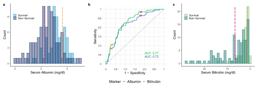
Figure 1: Traditional ROC curves for two biomedical markers, serum albumin and serum bilirubin, as predictors of patient survival beyond a threshold value of 1462 days (four years) in a Mayo Clinic trial. (a, c) Bar plots of marker levels conditional on survival or non-survival. The stronger shading results from overlap. For bilirubin, we reverse orientation, as is customary in the biomedical literature. (b) ROC curves and ${\rm AUC}$ values. The crosses correspond to binary classifiers at the feature thresholds indicated in the bar plots.

In this paper, we propose a powerful generalization of ROC analysis, which overcomes extant shortcomings, and introduce data science tools in the form of the ROC movie, the universal ROC (UROC) curve, and an associated, rank based coefficient of (potential) predictive ability (${\rm CPA}$) measure — tools that apply to just any linearly ordered outcome, including both binary, ordinal, mixed discrete-continuous, and continuous variables. The ROC movie comprises the sequence of the traditional, static ROC curves as the linearly ordered outcome is converted to a binary variable at successively higher thresholds. The UROC curve is a weighted average of the individual ROC curves that constitute the ROC movie, with weights that depend on the class configuration, as induced by the unique values of the outcome, in judiciously predicated, well-defined ways. ${\rm CPA}$ is a weighted average of the individual ${\rm AUC}$ values in the very same way that the UROC curve is a weighted average of the individual ROC curves that constitute the ROC movie. Hence, ${\rm CPA}$ equals the area under the UROC curve. This set of generalized tools reduces to the standard ROC curve and ${\rm AUC}$ when applied to binary outcomes. Moreover, key properties and relations from conventional ROC theory extend to ROC movies, UROC curves, and ${\rm CPA}$ in meaningful ways, to result in a coherent toolbox that properly extends the standard ROC concept. For a graphical preview, we return to the survival data example from Fig. 1, where the outcome was artificially made binary. Equipped with the new set of tools we no longer need to transform survival time into a specific dichotomous outcome. Figure 2 shows the ROC movie, the UROC curve, and ${\rm CPA}$ for the survival dataset.

The remainder of the paper is organized as follows. Section 2 provides a brief review of conventional ROC analysis for dichotomous outcomes. The key technical development is in Sections 3 and 4, where we introduce and study ROC movies, UROC curves, and the rank based ${\rm CPA}$ measure. To illustrate practical usage and relevance, real data examples from survival analysis and weather prediction are presented in Section 5. We monitor recent progress in numerical weather prediction (NWP) and shed new light on a recent comparison of the predictive abilities of convolutional neural networks (CNNs) vs. traditional NWP models. The paper closes with a discussion in Section 6.

[label = myAnim7, height = 70mm]7figures/imgeps4_out

Figure 2: ROC movies, UROC curves, and ${\rm CPA}$ for two biomedical markers, serum albumin and serum bilirubin, as predictors of patient survival (in days) in a Mayo Clinic trial. The ROC movies show the traditional ROC curves for binary events that correspond to patient survival beyond successively higher thresholds. The numbers at upper left show the current value of the threshold in days, at upper middle the respective relative weight, and at bottom right the ${\rm AUC}$ values. The threshold value of 1462 days recovers the traditional ROC curves in Fig. 1. The video ends in a static screen with the UROC curves and ${\rm CPA}$ values for the two markers.

2 Receiver operating characteristic (ROC) curves and area under the curve (AUC) for binary outcomes

Before we introduce ROC movies, UROC curves, and ${\rm CPA}$, it is essential that we establish notation and review the classical case of ROC analysis for binary outcomes, as described in review articles and monographs by Hanley and McNeil (1982), Swets (1988), Bradley (1997), Pepe (2003), Fawcett (2006), and Flach (2016), among others.

2.1 Binary setting

Throughout this section we consider bivariate data of the form

$$(x_{1},y_{1}),\ldots,(x_{n},y_{n})\,\in\,\times\{0,1\},$$ (1)

where $x_{i}\in$ is a real-valued classifier score, feature, marker, or covariate value, and $y_{i}\in\{0,1\}$ is a binary outcome, for $i=1,\ldots,n$. Following the extant literature, we refer to $y=1$ as the positive outcome and to $y=0$ as the negative outcome, and we assume that higher values of the feature are indicative of stronger support for the positive outcome. Throughout we assume that there is at least one index $i\in\{1,\ldots,n\}$ with $y_{i}=0$, and a further index $j\in\{1,\ldots,n\}$ with $y_{j}=1$.

2.2 Receiver operating characteristic (ROC) curves

We can use any threshold value $x\in$ to obtain a hard classifier, by predicting a positive outcome for a feature value $>x$, and predicting a negative outcome for a feature value $\leq x$. If we compare to the actual outcome, four possibilities arise. True positive and true negative cases correspond to correctly classified instances from class 1 and class 0, respectively. Similarly, false positive and false negative cases are misclassified instances from class 1 and class 0, respectively.

Considering the data (1), we obtain the respective true positive rate, hit rate or sensitivity (se),

$${\rm se}(x)=\frac{\frac{1}{n}\sum_{i=1}^{n}\mathbbm{1}\{x_{i}>x,\hskip 0.56905pty_{i}=1\}}{\frac{1}{n}\sum_{i=1}^{n}\mathbbm{1}\{\hskip 0.56905pty_{i}=1\}},$$

and the false negative rate, false alarm rate or one minus the specificity (sp),

$$1-{\rm sp}(x)=\frac{\frac{1}{n}\sum_{i=1}^{n}\mathbbm{1}\{x_{i}>x,\hskip 0.56905pty_{i}=0\}}{\frac{1}{n}\sum_{i=1}^{n}\mathbbm{1}\{\hskip 0.56905pty_{i}=0\}},$$

at the threshold value $x\in$, where the indicator $\mathbbm{1}\{A\}$ equals one if the event $A$ is true and zero otherwise.

Evidently, it suffices to consider threshold values $x$ equal to any of the unique values of $x_{1},\ldots,x_{n}$ or some $x_{0}<x_{1}$. For every $x$ of this form, we obtain a point

$$(1-{\rm sp}(x),{\rm se}(x))$$

in the unit square. Linear interpolation of the respective discrete point set results in a piecewise linear curve from $(0,0)$ to $(1,1)$ that is called the receiver operating characteristic (ROC) curve. For a mathematically oriented, detailed discussion of the construction see Section 2 of Gneiting and Vogel (2018).

2.3 Area under the curve (AUC)

The area under the ROC curve is a widely used measure of the predictive potential of a feature and generally referred to as the area under the curve (${\rm AUC}$).

In what follows, a well-known interpretation of ${\rm AUC}$ in terms of probabilities will be useful. To this end, we define the function

$$s(x,x^{\prime})=\mathbbm{1}\{x<x^{\prime}\}+\frac{1}{2}\mathbbm{1}\{x=x^{\prime}\},$$ (2)

where $x,x^{\prime}\in$. For subsequent use, note that if $x$ and $x^{\prime}$ are ranked within a list, and ties are resolved by assigning equal ranks within tied groups, then $s(x,x^{\prime})=s({\rm rk}(x),{\rm rk}(x^{\prime}))$, where ${\rm rk}(x)$ and ${\rm rk}(x^{\prime})$ are the ranks of $x$ and $x^{\prime}$.

We now change notation and refer to the feature values in class $i\in\{0,1\}$ as $x_{ik}$ for $k=1,\ldots,n_{i}$, where $n_{0}=\sum_{i=1}^{n}\mathbbm{1}\{y_{i}=0\}$ and $n_{1}=\sum_{i=1}^{n}\mathbbm{1}\{y_{i}=1\}$, respectively. Thus, we have rewritten (1) as

$$(x_{01},0),\ldots,(x_{0n_{0}},0),(x_{11},1),\ldots,(x_{1n_{1}},1)\,\in\,\times\{0,1\}.$$ (3)

Using the new notation, Result 4.10 of Pepe (2003) states that

$${\rm AUC}=\frac{1}{n_{0}n_{1}}\,\sum_{i=1}^{n_{0}}\sum_{j=1}^{n_{1}}s(x_{0i},x_{1j}).$$ (4)

In words, ${\rm AUC}$ equals the probability that under random sampling a feature value from a positive instance is greater than a feature value from a negative instance, with any ties resolved at random. Expressed differently, ${\rm AUC}$ equals the tie-adjusted probability of concordance in feature–outcome pairs, where we define instances $(x,y)\in^{2}$ and $(x^{\prime},y^{\prime})\in^{2}$ with $y\not=y^{\prime}$ to be concordant if either $x>x^{\prime}$ and $y>y^{\prime}$, or $x<x^{\prime}$ and $y<y^{\prime}$. Similarly, instances $(x,y)$ and $(x^{\prime},y^{\prime})$ with $y\not=y^{\prime}$ are discordant if either $x>x^{\prime}$ and $y<y^{\prime}$, or $x<x^{\prime}$ and $y>y^{\prime}$.

Further investigation reveals a close connection to Somers’ $D$, a classical measure of ordinal association (Somers, 1962). This measure is defined as

$$D=\frac{n_{c}-n_{d}}{n_{0}n_{1}},$$

where $n_{0}n_{1}$ is the total number of pairs with distinct outcomes that arise from the data in (3), $n_{c}$ is the number of concordant pairs, and $n_{d}$ is the number of discordant pairs. Finally, let $n_{e}$ be the number of pairs for which the feature values are equal. The relationship (4) yields

$${\rm AUC}=\frac{n_{c}}{n_{0}n_{1}}+\frac{1}{2}\frac{n_{e}}{n_{0}n_{1}},$$

and as $n_{0}n_{1}=n_{c}+n_{d}+n_{e}$, it follows that

$${\rm AUC}=\frac{1}{2}\left(D+1\right)$$ (5)

relates linearly to Somers’ $D$.

To give an example, suppose that the real-valued outcome $Y$ and the features $X$, $X^{\prime}$ and $X^{\prime\prime}$ are jointly Gaussian. Specifically, we assume that the joint distribution of $(Y,X,X^{\prime},X^{\prime\prime})$ is multivariate normal with covariance matrix

$$\begin{pmatrix}1&0.8&0.5&0.2\\ 0.8&1&0.8&0.5\\ 0.5&0.8&1&0.8\\ 0.2&0.5&0.8&1\\ \end{pmatrix}.$$ (6)

In order to apply classical ROC analysis, the real-valued outcome $Y$ needs to be converted to a binary variable, namely, an event of the type $Y_{\theta}=\mathbbm{1}\{Y\geq\theta\}$ of $Y$ being greater than or equal to a threshold value $\theta$. Figure 3 shows ROC curves for the features $X$, $X^{\prime}$ and $X^{\prime\prime}$ as a predictor of the binary variable $Y_{1}$, based on a sample of size $n=400$. The ${\rm AUC}$ values for $X$, $X^{\prime}$ and $X^{\prime\prime}$ as a predictor of $Y_{1}$ are .91, .72 and .61, respectively.

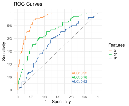
Figure 3: Traditional ROC curves and ${\rm AUC}$ values for the features $X$, $X^{\prime}$ and $X^{\prime\prime}$ as predictors of the binary outcome $Y_{1}=\mathbbm{1}\{Y\geq 1\}$ in the simulation example of Section 2.3, based on a sample of size $n=400$.

2.4 Key properties

A key requirement for a persuasive generalization of classical ROC analysis is the reduction to ROC curves and ${\rm AUC}$ if the outcomes are binary. Furthermore, well established desirable properties from ROC analysis ought to be retained. To facilitate judging whether the generalization in Sections 3 and 4 satisfies these desiderata, we summarize key properties of ROC curves and ${\rm AUC}$ in the following (slightly informal) listing.

• The ROC curve and ${\rm AUC}$ are straightforward to compute and interpret, in the (rough) sense of the larger the better.

• ${\rm AUC}$ attains values between 0 and 1 and relates linearly to Somers’ $D$. For a perfect feature, ${\rm AUC}=1$ and $D=1$; for a feature that is independent of the binary outcome, ${\rm AUC}=\frac{1}{2}$ und $D=0$.

• The numerical value of ${\rm AUC}$ admits an interpretation as the probability of concordance for feature–outcome pairs.

• The ROC curve and ${\rm AUC}$ are purely rank based and, therefore, invariant under strictly increasing transformations. Specifically, if $\phi:\to$ is a strictly increasing function, then the ROC curve and ${\rm AUC}$ computed from

  $$(\phi(x_{1}),y_{1}),\ldots,(\phi(x_{n}),y_{n})\,\in\,\times\{0,1\}$$ (7)

  are the same as the ROC curve and ${\rm AUC}$ computed from (1).

As an immediate consequence of the latter property, ROC curves and ${\rm AUC}$ assess the discrimination ability or potential predictive ability of a classifier, feature, marker, or test (Wilks, 2019). Distinctly different methods are called for if one seeks to evaluate a classifier’s actual value in any given applied setting (Adams and Hands, 1999; Hernández-Orallo et al., 2012; Ehm et al., 2016).

3 ROC movies and universal ROC (UROC) curves for real-valued outcomes

As noted, traditional ROC analysis applies to binary outcomes only. Thus, researchers working with real-valued outcomes, and desiring to apply ROC analysis, need to convert and reduce to binary outcomes, by thresholding artificially at a cut-off value. Here we propose a powerful generalization of ROC analysis, which overcomes extant shortcomings, and introduce data analytic tools in the form of the ROC movie, the universal ROC (UROC) curve, and an associated rank based coefficient of (potential) predictive ability (${\rm CPA}$) measure — tools that apply to just any linearly ordered outcome, including both binary, ordinal, mixed discrete-continuous, and continuous variables.

3.1 General real-valued setting

Generalizing the binary setting in (1), we now consider bivariate data of the form

$$(x_{1},y_{1}),\ldots,(x_{n},y_{n})\,\in\,\times,$$ (8)

where $x_{i}$ is a real-valued point forecast, regression output, feature, marker, or covariate value, and $y_{i}$ is a real-valued outcome, for $i=1,\ldots,n$. Throughout we assume that there are at least two unique values among the outcomes $y_{1},\ldots,y_{n}$.

The crux of the subsequent development lies in a conversion to a sequence of binary problems. To this end, we let

$$z_{1}<\cdots<z_{m}$$

denote the $m\leq n$ unique values of $y_{1},\ldots,y_{n}$, and we define

$$n_{c}=\sum_{i=1}^{n}\mathbbm{1}\{y_{i}=z_{c}\}$$

as the number of instances among the outcomes $y_{1},\ldots,y_{n}$ that equal $z_{c}$, for $c=1,\ldots,m$, so that $n_{1}+\cdots+n_{m}=n$. We refer to the respective groups of instances as classes.

Next we transform the real-valued outcomes $y_{1},\ldots,y_{n}$ into binary outcomes $\mathbbm{1}\{y_{1}\geq\theta\},\ldots,\mathbbm{1}\{y_{n}\geq\theta\}$ relative to a threshold value $\theta\in$. Thus, instead of analysing the original problem in (8), we consider a series of binary problems. By construction, only values of $\theta$ equal to $z_{2},\ldots,z_{m}$ result in nontrivial, unique sets of binary outcomes. Therefore, we consider $m-1$ derived classification problems with binary data of the form

$$(x_{1},\mathbbm{1}\{y_{1}\geq z_{c+1}\}),\ldots,(x_{n},\mathbbm{1}\{y_{n}\geq z_{c+1}\})\,\in\,\times\{0,1\},$$ (9)

where $c=1,\ldots,m-1$. As the derived problems are binary, all the tools of traditional ROC analysis apply.

In the remainder of the section we describe our generalization of ROC curves for binary data to ROC movies and universal ROC (UROC) curves for real-valued data. First, we argue that the $m-1$ classical ROC curves for the derived data in (9) can be merged into a single dynamical display, to which we refer as a ROC movie (Definition 1). Then we define the UROC curve as a judiciously weighted average of the classical ROC curves of which the ROC movie is composed (Definition 2).

Finally, we introduce a general measure of potential predictive ability for features, termed the coefficient of predictive ability (CPA). ${\rm CPA}$ is a weighted average of the ${\rm AUC}$ values for the derived binary problems in the very same way that the UROC curve is a weighted average of the (classical) ROC curves that constitute the ROC movie. Hence, ${\rm CPA}$ equals the area under the UROC curve (Definition 3). Alternatively, ${\rm CPA}$ can be interpreted as a weighted probability of concordance (Theorem 1) or in terms of rank based covariances (Theorem 2). ${\rm CPA}$ reduces to ${\rm AUC}$ if the outcomes are binary, and relates linearly to Spearman’s rank correlation coefficient if the outcomes are continuous (Theorems 3 and 4).

3.2 ROC movies

We consider the sequence of $m-1$ classification problems for the derived binary data in (9). For $c=1,\ldots,m-1$, we let ${\rm ROC}_{c}$ denote the associated ROC curve, and we let ${\rm AUC}_{c}$ be the respective ${\rm AUC}$ value.

Definition 1.

For data of the form (8), the ROC movie is the sequence $({\rm ROC}_{c})_{c=1,\ldots,m-1}$ of the ROC curves for the induced binary data in (9).

If the original problem is binary there are $m=2$ classes only, and the ROC movie reduces to the classical ROC curve. In case the outcome attains $m\geq 3$ distinct values the ROC movie can be visualized by displaying the associated sequence of $m-1$ ROC curves. In medical survival analysis, the outcomes $y_{1},\ldots,y_{n}$ in data of the form (8) are survival times, and the analysis is frequently hampered by censoring, as patients drop out of studies. In this setting, Etzioni et al. (1999) and Heagerty et al. (2000) introduced the notion of time-dependent ROC curves, which are classical ROC curves for the binary indicator $\mathbbm{1}\{y_{i}\geq t\}$ of survival through (follow-up) time $t$, with censoring being handled efficiently. For an example see Fig. 2 of Heagerty et al. (2000), where the ROC curves concern survival beyond follow-up times of 40, 60, and 100 months, respectively. If the thresholds considered correspond to the unique values of the outcomes, the sequence of time-dependent ROC curves becomes a ROC movie in the sense of Definition 1, save for the handling of censored data. When the number $m\leq n$ of classes is small or modest, the generation of the ROC movie is straightforward. Adaptations might be required as $m$ grows, and we tend to this question in Section 5.2.

[label = myAnim7, height = 70mm]28figures/imgeps3_reduced0

Figure 4: ROC movies and UROC curves for the features $X$, $X^{\prime}$ and $X^{\prime\prime}$ as predictors of the real-valued outcome $Y$ in the simulation example of Section 2.3, based on the same sample as in Fig. 3. In the ROC movies, the number at upper left shows the threshold under consideration, the number at upper center the relative weight $w_{c}/\max_{l=1,\ldots,m-1}w_{l}$ from (11), and the numbers at bottom right the respective ${\rm AUC}$ values.

We have implemented ROC movies, UROC curves, and ${\rm CPA}$ within the uroc package for the statistical programming language R (R Core Team, 2021) where the animation package of Xie (2013) provides functionality for converting R images into a GIF animation, based on the external software ImageMagick. The uroc package can be downloaded from https://github.com/evwalz/uroc. In addition, a Python (Python, 2021) implementation is available at https://github.com/evwalz/urocc. Returning to the example of Section 2.3, Fig. 4 compares the features $X$, $X^{\prime}$ and $X^{\prime\prime}$ as predictors of the real-valued outcome $Y$ in a joint display of the three ROC movies and UROC curves, based on the same sample of size $n=400$ as in Fig. 3. In the ROC movies, the threshold $z=1.00$ recovers the traditional ROC curves in Fig. 3.

3.3 Universal ROC (UROC) curves

Next we propose a simple and efficient way of subsuming a ROC movie for data of the form (8) into a single, static graphical display. As before, let $z_{1}<\cdots<z_{m}$ denote the unique values of $y_{1},\ldots,y_{n}$, let $n_{c}=\sum_{i=1}^{n}\mathbbm{1}\{y_{i}=z_{c}\}$, and let ${\rm ROC}_{c}$ denote the (classical) ROC curve associated with the binary problem in (9), for $c=1,\ldots,m-1$.

By Theorem 5 of Gneiting and Vogel (2018), there is a natural bijection between the class of the ROC curves and the class of the cumulative distribution functions (CDFs) of Borel probability measures on the unit interval. In particular, any ROC curve can be associated with a non-decreasing, right-continuous function $R:[0,1]\to[0,1]$ such that $R(0)=0$ and $R(1)=1$. Hence, any convex combination of the ROC curves ${\rm ROC}_{1},\ldots,{\rm ROC}_{m-1}$ can also be associated with a non-decreasing, right-continuous function on the unit interval. It is in this sense that we define the following; in a nutshell, the UROC curve averages the traditional ROC curves of which the ROC movie is composed.

Definition 2.

For data of the form (8), the universal receiver operating characteristic (UROC) curve is the curve associated with the function

$$\sum_{c=1}^{m-1}w_{c}\,{\rm ROC}_{c}$$ (10)

on the unit interval, with weights

$$w_{c}=\left.\left(\,\sum_{i=1}^{c}n_{i}\sum_{i=c+1}^{m}n_{i}\right)\right/\left(\sum_{i=1}^{m-1}\sum_{j=i+1}^{m}(\hskip 0.56905ptj-i)\hskip 0.56905ptn_{i}n_{j}\right)$$ (11)

for $c=1,\ldots,m-1$.

Importantly, the weights in (11) depend on the data in (8) via the outcomes $y_{1},\ldots,y_{n}$ only. Thus, they are independent of the feature values and can be used meaningfully in order to compare and rank features. Their specific choice is justified in Theorems 1 and 2 below. Clearly, the weights are nonnegative and sum to one. If $m=n$ then $n_{1}=\cdots=n_{m}=1$, and (11) reduces to

$$w_{c}=6\,\frac{c(n-c)}{n(n^{2}-1)}\quad{\rm for}\quad c=1,\ldots,n-1;$$ (12)

so the weights are quadratic in the rank $c$ and symmetric about the inner most rank(s), at which they attain a maximum. As we will see, our choice of weights has the effect that in this setting the area under the UROC curve, to which we refer as a general coefficient of predictive ability (${\rm CPA}$), relates linearly to Spearman’s rank correlation coefficient, in the same way that ${\rm AUC}$ relates linearly to Somers’ $D$.

In Fig. 4 the UROC curves appear in the final static screen, subsequent to the ROC movies. Within each ROC movie, the individual frames show the ROC curve ${\rm ROC}_{c}$ for the feature considered. Furthermore, we display the threshold $z_{c}$, the relative weight from (11) (the actual weight normalized to the unit interval, i.e., we show $w_{c}/\max_{l=1,\ldots,m-1}w_{l}$), and ${\rm AUC}_{c}$, respectively, for $c=1,\ldots,m-1$. Once more we emphasize that the use of ROC movies, UROC curves, and ${\rm CPA}$ frees researchers from the need to select — typically, arbitrary — threshold values and binarize, as mandated by classical ROC analysis.

Of course, if specific threshold values are of particular substantive interest, the respective ROC curves can be extracted from the ROC movie, and it can be useful to plot ${\rm AUC}_{c}$ versus the associated threshold value $z_{c}$. Displays of this type have been introduced and studied by Rosset et al. (2005).

4 Coefficient of predictive ability (${\rm CPA}$)

We proceed to define the coefficient of predictive ability (${\rm CPA}$) as a general measure of potential predictive ability, based on notation introduced in Sections 3.2 and 3.3.

Definition 3.

For data of the form (8) and weights $w_{1},\ldots,w_{m-1}$ as in (11), the coefficient of predictive ability (${\rm CPA}$) is defined as

$${\rm CPA}=\sum_{c=1}^{m-1}w_{c}\,{\rm AUC}_{c}.$$ (13)

In words, ${\rm CPA}$ equals the area under the UROC curve.

Importantly, ROC movies, UROC curves, and ${\rm CPA}$ satisfy a fundamental requirement on any generalization of ROC curves and ${\rm AUC}$, in that they reduce to the classical notions when applied to a binary problem, whence $m=2$ in (10) and (13), respectively. Another requirement that we consider essential is that, when both the feature values $x_{1},\ldots,x_{n}$ and the outcomes $y_{1},\ldots,y_{n}$ are pairwise distinct, the value of a performance measure remains unchanged if we transpose the roles of the feature and the outcome. As we will see, this is true under our specific choice (11) of the weights $w_{c}$ in the defining formula (13) for ${\rm CPA}$, but is not true under other choices, such as in the case of equal weights.

4.1 Interpretation as a weighted probability

We now express ${\rm CPA}$ in terms of pairwise comparisons via the function $s$ in (2). To this end, we usefully change notation for the data in (8) and refer to the feature values in class $c\in\{1,\ldots,m\}$ as $x_{ck}$, for $k=1,\ldots,n_{c}$. Thus, we rewrite (8) as

$$(x_{11},z_{1}),\ldots,(x_{1n_{1}},z_{1}),\,\ldots,\,(x_{m1},z_{m}),\ldots,(x_{mn_{m}},z_{m})\,\in\,\times,$$ (14)

where $z_{1}<\cdots<z_{m}$ are the unique values of $y_{1},\ldots,y_{n}$ and $n_{c}=\sum_{i=1}^{n}\mathbbm{1}\{y_{i}=z_{c}\}$, for $c=1,\ldots,m$.

Theorem 1.

For data of the form (14),

$${\rm CPA}=\frac{\sum_{i=1}^{m-1}\sum_{j=i+1}^{m}\sum_{k=1}^{n_{i}}\sum_{l=1}^{n_{j}}(\hskip 0.56905ptj-i)\,s(x_{ik},x_{jl})}{\sum_{i=1}^{m-1}\sum_{j=i+1}^{m}(\hskip 0.56905ptj-i)\,n_{i}n_{j}}.$$ (15)

Proof.

By (4), the individual ${\rm AUC}$ values satisfy

$${\rm AUC}_{c}=\frac{1}{\sum_{i=1}^{c}n_{i}\sum_{i=c+1}^{m}n_{i}}\sum_{i=1}^{c}\sum_{j=c+1}^{m}\sum_{k=1}^{n_{i}}\sum_{l=1}^{n_{j}}s(x_{ik},x_{jl})$$

for $c=1,\ldots,m-1$. In view of (11) and (13), summation yields

$${\rm CPA} =\sum_{c=1}^{m-1}w_{c}\,{\rm AUC}_{c}$$

$$=\frac{\sum_{c=1}^{m-1}\sum_{i=1}^{c}\sum_{j=c+1}^{m}\sum_{k=1}^{n_{i}}\sum_{l=1}^{n_{j}}s(x_{ik},x_{jl})}{\sum_{i=1}^{m-1}\sum_{j=i+1}^{m}(\hskip 0.56905ptj-i)\,n_{i}n_{j}}$$

$$=\frac{\sum_{i=1}^{m-1}\sum_{j=i+1}^{m}\sum_{k=1}^{n_{i}}\sum_{l=1}^{n_{j}}(\hskip 0.56905ptj-i)\,s(x_{ik},x_{jl})}{\sum_{i=1}^{m-1}\sum_{j=i+1}^{m}(\hskip 0.56905ptj-i)\,n_{i}n_{j}},$$

as claimed. ∎

Thus, ${\rm CPA}$ is based on pairwise comparisons of feature values, counting the number of concordant pairs in (14), adjusting to a count of $\frac{1}{2}$ if feature values are tied, and weighting a pair’s contribution by a class based distance, $j-i$, between the respective outcomes, $z_{j}>z_{i}$. In other words, ${\rm CPA}$ equals a weighted probability of concordance, with weights that grow linearly in the class based distance between outcomes.

The specific form of ${\rm CPA}$ in (15) invites comparison to a widely used measure of discrimination in biomedical applications, namely, the C index (Harrell et al., 1996; Pencina and D’Agostino, 2004)

$${\rm C}=\frac{\sum_{i=1}^{m-1}\sum_{j=i+1}^{m}\sum_{k=1}^{n_{i}}\sum_{l=1}^{n_{j}}s(x_{ik},x_{jl})}{\sum_{i=1}^{m-1}\sum_{j=i+1}^{m}n_{i}n_{j}}.$$ (16)

If the outcomes are binary, both the C index and ${\rm CPA}$ reduce to ${\rm AUC}$. While ${\rm CPA}$ can be interpreted as a weighted probability of concordance, C admits an interpretation as an unweighted probability, whence Mason and Weigel (2009) recommend its use for administrative purposes. However, the weighting in (15) may be more meaningful, as concordance between feature–outcome pairs with outcomes that differ substantially in rank tends to be of greater practical relevance than concordance between pairs with alike outcomes. While ${\rm CPA}$ admits the appealing, equivalent interpretation (13) in terms of binary ${\rm AUC}$ values and the area under the UROC curve, relationships of this type are unavailable for the C index.

Subject to conditions, the C index relates linearly to Kendall’s rank correlation coefficient (Somers, 1962; Pencina and D’Agostino, 2004; Mason and Weigel, 2009). In Section 4.3 we demonstrate the same type of relationship for ${\rm CPA}$ and Spearman’s rank correlation coefficient, thereby resolving a problem raised by Heagerty and Zheng (2005, p. 95). Just as the C index bridges and generalizes ${\rm AUC}$ and Kendall’s coefficient, ${\rm CPA}$ bridges and nests ${\rm AUC}$ and Spearman’s coefficient, with the added benefit of appealing interpretations in terms of the area under the UROC curve and rank based covariances.

4.2 Representation in terms of covariances

The key result in this section represents ${\rm CPA}$ in terms of the covariance between the class of the outcome and the mid rank of the feature, relative to the covariance between the class of the outcome and the mid rank of the outcome itself.

The mid rank method handles ties by assigning the arithmetic average of the ranks involved (Woodbury, 1940; Kruskal, 1958). For instance, if the third to seventh positions in a list are tied, their shared mid rank is $\frac{1}{5}(3+4+5+6+7)=5$. This approach treats equal values alike and guarantees that the sum of the ranks in any tied group is unchanged from the case of no ties. As before, if $y_{i}=z_{j}$, where $z_{1}<\cdots<z_{m}$ are the unique values of $y_{1},\ldots,y_{n}$ in (8), we say that the class of $y_{i}$ is $j$. In brief, we express this as ${\rm cl}(y_{i})=j$. Similarly, we refer to the mid rank of $x_{i}$ within $x_{1},\ldots,x_{n}$ as $\overline{{\rm rk}}(x_{i})$.

Theorem 2.

Let the random vector $(X,Y)$ be drawn from the empirical distribution of the data in (8) or (14). Then

$${\rm CPA}=\frac{1}{2}\left(\frac{{\rm cov}({\rm cl}(Y),\overline{{\rm rk}}(X))}{{\rm cov}({\rm cl}(Y),\overline{{\rm rk}}(Y))}+1\right).$$ (17)

Proof.

Suppose that the law of the random vector $(X,Y)$ is the empirical distribution of the data in (8). Based on the equivalent representation in (14), we find that

$$\frac{{\rm cov}({\rm cl}(Y),\overline{{\rm rk}}(X))}{{\rm cov}({\rm cl}(Y),\overline{{\rm rk}}(Y))}=\frac{\sum_{i=1}^{m}\sum_{k=1}^{n_{i}}i\hskip 0.56905pt\hskip 0.56905pt\overline{{\rm rk}}(x_{ik})-\frac{1}{2}\hskip 0.56905pt(n+1)\sum_{i=1}^{m}i\hskip 0.56905ptn_{i}}{\sum_{i=1}^{m}i\hskip 0.56905ptn_{i}\left(\sum_{j=0}^{i-1}n_{j}+\frac{1}{2}(n_{i}+1)\right)-\frac{1}{2}\hskip 0.56905pt(n+1)\sum_{i=1}^{m}i\hskip 0.56905ptn_{i}},$$

where $n_{0}=0$. Consequently, we can rewrite (17) as

$${\rm CPA}=\frac{\sum_{i=1}^{m}\sum_{k=1}^{n_{i}}i\hskip 0.56905pt\hskip 0.56905pt\overline{{\rm rk}}(x_{ik})+\sum_{i=1}^{m}i\hskip 0.56905ptn_{i}\left(\sum_{j=0}^{i-1}n_{j}+\frac{1}{2}n_{i}-n-\frac{1}{2}\right)}{\sum_{i=1}^{m}i\hskip 0.56905ptn_{i}\left(2\hskip 0.56905pt\sum_{j=0}^{i-1}n_{j}+n_{i}-n\right)}.$$ (18)

We proceed to demonstrate that the numerator and denominator in (15) equal the numerator and denominator in (18), respectively. To this end, we first compare feature values within classes and note that

$$\sum_{i=1}^{m}\sum_{k=1}^{n_{i}}\sum_{l=1}^{n_{i}}i\hskip 0.56905pts(x_{il},x_{ik})=\sum_{i=1}^{m}i\sum_{k=1}^{n_{i}}\left(n_{i}-k+\frac{1}{2}\right)=\frac{1}{2}\sum_{i=1}^{m}i\hskip 0.56905ptn_{i}^{2};$$

for if the feature values in class $i$ are all distinct, the largest one exceeds $n_{i}-1$ others, the second largest exceeds $n_{i}-2$ others, and so on, and analogously in case of ties. We now show the equality of the numerators in (15) and (18), in that

$$\sum_{i=1}^{m-1}\sum_{j=i+1}^{m}\sum_{k=1}^{n_{i}}\sum_{l=1}^{n_{j}}(\hskip 0.56905ptj-i)\,s(x_{ik},x_{jl})$$

$$=\sum_{i=1}^{m-1}\sum_{j=i+1}^{m}\sum_{k=1}^{n_{i}}\sum_{l=1}^{n_{j}}j\hskip 0.56905pts(x_{ik},x_{jl})-\sum_{i=1}^{m-1}\sum_{j=i+1}^{m}\sum_{k=1}^{n_{i}}\sum_{l=1}^{n_{j}}i\hskip 0.56905pts(x_{ik},x_{jl})$$

$$\hskip 56.9055pt+\sum_{j=1}^{m-1}\sum_{i=j+1}^{m}\sum_{k=1}^{n_{j}}\sum_{l=1}^{n_{i}}j\hskip 0.56905pts(x_{ik},x_{jl})-\sum_{j=1}^{m-1}\sum_{i=j+1}^{m}\sum_{k=1}^{n_{j}}\sum_{l=1}^{n_{i}}j\hskip 0.56905pts(x_{ik},x_{jl})$$

$$=\sum_{i=1}^{m}\sum_{\begin{subarray}{c}j=1\\ j\neq i\end{subarray}}^{m}\sum_{k=1}^{n_{i}}\sum_{l=1}^{n_{j}}j\hskip 0.56905pts(x_{ik},x_{jl})-\sum_{i=1}^{m-1}\sum_{j=i+1}^{m}\sum_{k=1}^{n_{i}}\sum_{l=1}^{n_{j}}i\left(s(x_{jl},x_{ik})+s(x_{ik},x_{jl})\right)$$

$$=\sum_{j=1}^{m}\sum_{l=1}^{n_{j}}j\left(\hskip 0.56905pt\overline{{\rm rk}}(x_{jl})-\frac{1}{2}\right)-\sum_{i=1}^{m}\sum_{k=1}^{n_{i}}\sum_{l=1}^{n_{i}}i\hskip 0.56905pts(x_{il},x_{ik})-\sum_{i=1}^{m-1}\sum_{j=i+1}^{m}i\hskip 0.56905ptn_{i}n_{j}$$

$$=\sum_{i=1}^{m}\sum_{k=1}^{n_{i}}i\hskip 0.56905pt\overline{{\rm rk}}(x_{ik)}-\frac{1}{2}\sum_{i=1}^{m}i\hskip 0.56905ptn_{i}-\frac{1}{2}\sum_{i=1}^{m}i\hskip 0.56905ptn_{i}^{2}-n\sum_{i=1}^{m-1}i\hskip 0.56905ptn_{i}+\sum_{i=1}^{m-1}i\hskip 0.56905ptn_{i}\sum_{j=0}^{i}n_{j}$$

$$=\sum_{i=1}^{m}\sum_{k=1}^{n_{i}}i\hskip 0.56905pt\overline{{\rm rk}}(x_{ik)}-\frac{1}{2}\sum_{i=1}^{m}i\hskip 0.56905ptn_{i}-\frac{1}{2}\sum_{i=1}^{m}i\hskip 0.56905ptn_{i}^{2}-n\sum_{i=1}^{m}i\hskip 0.56905ptn_{i}+\sum_{i=1}^{m}i\hskip 0.56905ptn_{i}\sum_{j=0}^{i}n_{j}$$

$$=\sum_{i=1}^{m}\sum_{k=1}^{n_{i}}i\hskip 0.56905pt\overline{{\rm rk}}(x_{ik)}+\sum_{i=1}^{m}i\hskip 0.56905ptn_{i}\left(\sum_{j=0}^{i-1}n_{j}+\frac{1}{2}n_{i}-n-\frac{1}{2}\right).$$

As for the denominators,

$$\sum_{i=1}^{m-1}\sum_{j=i+1}^{m}(\hskip 0.56905ptj-i)\,n_{i}n_{j}=\sum_{i=1}^{m-1}\sum_{j=i+1}^{m}j\hskip 0.56905ptn_{i}n_{j}-\sum_{i=1}^{m-1}\sum_{j=i+1}^{m}i\hskip 0.56905ptn_{i}n_{j}$$

$$\hskip 11.38109pt=\sum_{i=1}^{m}i\hskip 0.56905ptn_{i}\sum_{k=0}^{i-1}n_{k}-n\sum_{i=1}^{m-1}i\hskip 0.56905ptn_{i}+\sum_{i=1}^{m-1}i\hskip 0.56905ptn_{i}\sum_{k=1}^{i}n_{k}$$

$$\hskip 11.38109pt=2\sum_{i=1}^{m}in_{i}\sum_{k=0}^{i-1}n_{k}-n\sum_{i=1}^{m-1}i\hskip 0.56905ptn_{i}+\sum_{i=1}^{m-1}i\hskip 0.56905ptn_{i}^{2}+\sum_{i=1}^{m-1}i\hskip 0.56905ptn_{i}\sum_{k=0}^{i-1}n_{k}-\sum_{i=1}^{m}i\hskip 0.56905ptn_{i}\sum_{k=0}^{i-1}n_{k}$$

$$\hskip 11.38109pt=2\sum_{i=1}^{m}i\hskip 0.56905ptn_{i}\sum_{k=0}^{i-1}n_{k}-n\sum_{i=1}^{m-1}i\hskip 0.56905ptn_{i}+\sum_{i=1}^{m-1}i\hskip 0.56905ptn_{i}^{2}-nmn_{m}+mn_{m}^{2}$$

$$\hskip 11.38109pt=2\sum_{i=1}^{m}i\hskip 0.56905ptn_{i}\sum_{k=0}^{i-1}n_{k}-n\sum_{i=1}^{m}i\hskip 0.56905ptn_{i}+\sum_{i=1}^{m}i\hskip 0.56905ptn_{i}^{2}$$

$$\hskip 11.38109pt=\sum_{i=1}^{m}i\hskip 0.56905ptn_{i}\left(2\hskip 0.56905pt\sum_{j=0}^{i-1}n_{j}+n_{i}-n\right),$$

whence the proof is complete. ∎

Interestingly, the representation (17) in terms of rank and class based covariances appears to be new even in the special case when the outcomes are binary, so that ${\rm CPA}$ reduces to ${\rm AUC}$. The representation also sheds new light on the asymmetry of ${\rm CPA}$, in that, in general, the value of ${\rm CPA}$ changes if we transpose the roles of the feature and the outcome. In contrast to customarily used measures of bivariate association and dependence, which are necessarily symmetric (Nešlehová, 2007; Reshef et al., 2011; Weihs et al., 2018), ${\rm CPA}$ is directed when the outcome is binary or ordinal. Thus, ${\rm CPA}$ avoids a technical issue with the use of rank-based correlation coefficients in discrete settings, namely, that perfect classifiers do not reach the optimal values of the respective performance measures (Nešlehová, 2007, p. 565). However, in the case of no ties at all, to which we tend now, ${\rm CPA}$ becomes symmetric, as one would expect, given that the feature and the outcome are on equal footing then.

4.3 Relationship to Spearman’s rank correlation coefficient

Spearman’s rank correlation coefficient $\rho_{\scriptstyle\rm S}$ for data of the form (8) is generally understood as Pearson’s correlation coefficient applied to the respective ranks (Spearman, 1904). In case there are no ties in either $x_{1},\ldots,x_{n}$ nor $y_{1},\ldots,y_{n}$, the concept is unambiguous, and Spearman’s coefficient can be computed as

$$\rho_{\scriptstyle\rm S}=1-\frac{6}{n(n^{2}-1)}\sum_{i=1}^{n}\left({\rm rk}(x_{i})-{\rm rk}(y_{i})\right)^{2},$$ (19)

where ${\rm rk}(x_{i})$ denotes the rank of $x_{i}$ within $x_{1},\ldots,x_{n}$, and ${\rm rk}(y_{i})$ the rank of $y_{i}$ within $y_{1},\ldots,y_{n}$,

In this setting CPA relates linearly to Spearman’s rank correlation coefficient $\rho_{\scriptstyle\rm S}$, in the very same way that ${\rm AUC}$ relates to Somers’ $D$ in (5).

Theorem 3.

In the case of no ties,

$${\rm CPA}=\frac{1}{2}\left(\hskip 0.56905pt\rho_{\scriptstyle\rm S}+1\right).$$ (20)

Indeed, in case there are no ties, both mid ranks and classes reduce to ranks proper, and then (20) is readily identified as a special case of (17). For an alternative proof, in the absence of ties the weights $w_{c}$ in (11) are of the form (12). The stated result then follows upon combining the defining equation (10), the equality stated at the bottom of the left column of page 4 in Rosset et al. (2005), and equation (5) in the same reference.

Note that ${\rm CPA}$ becomes symmetric in this case, as its value remains unchanged if we transpose the roles of the feature and the outcome. Furthermore, if the joint distribution of a bivariate random vector $(X,Y)$ is continuous, and we think of the data in (8) as a sample from the respective population, then, by applying Definition 3 and Theorem 3 in the large sample limit, and taking (12) into account, we (informally) obtain a population version of ${\rm CPA}$, namely,

$${\rm CPA}=6\int_{0}^{1}\alpha(1-\alpha)\,{\rm AUC}_{\alpha}\,\rm{d}\alpha=\frac{1}{2}\left(\hskip 0.56905pt\rho_{\scriptstyle\rm S}+1\right),$$ (21)

where ${\rm AUC}_{\alpha}$ is the population version of ${\rm AUC}$ for $(X,\mathbbm{1}\{Y\geq q_{\alpha}\})$, with $q_{\alpha}$ denoting the $\alpha$-quantile of the marginal law of $Y$. We defer a rigorous derivation of (21) to future work and stress that, as both $X$ and $Y$ are continuous here, their roles can be interchanged.

Under the assumption of multivariate normality, the population version of Spearman’s $\rho_{\scriptstyle\rm S}$ relates to Pearson’s correlation coefficient $r$ as

$$\rho_{\scriptstyle\rm S}=\frac{6}{\pi}\arcsin\frac{r}{2};$$ (22)

see, e.g., Kruskal (1958). Returning to the example in Section 2.3, where $(Y,X,X^{\prime},X^{\prime\prime})$ is jointly Gaussian with covariance matrix (6), Table 1 states, for each feature, the population values of Pearson’s correlation coefficient $r$, ${\rm CPA}$, and the C index relative to the real-valued outcome $Y$, as derived from (21) and (22) and the respective relationships for the C index and Kendall’s rank correlation coefficient $\tau_{\scriptstyle\hskip 0.56905pt\rm K}$, namely

$${\rm C}=\frac{1}{2}\left(\hskip 0.56905pt\tau_{\scriptstyle\hskip 0.56905pt\rm K}+1\right)$$ (23)

and

$$\tau_{\scriptstyle\hskip 0.56905pt\rm K}=\frac{2}{\pi}\arcsin r.$$ (24)

These results imply that for a bivariate Gaussian population with Pearson correlation coefficient $r\in(0,1)$ it is true that $\tau_{\scriptstyle\hskip 0.56905pt\rm K}>\rho_{\scriptstyle\rm S}>0$ and ${\rm CPA}>{\rm C}>1/2$. In fact, under positive dependence it always holds that $\tau_{\scriptstyle\hskip 0.56905pt\rm K}\geq\rho_{\scriptstyle\rm S}\geq 0$, as demonstrated by Capéraà and Genest (1993), whence ${\rm CPA}\geq{\rm C}\geq 1/2$. However, there are also settings where these inequalities get violated (Schreyer et al, 2017). In Fig. 4 the ${\rm CPA}$ values for the features appear along with the UROC curves in the final static screen, subsequent to the ROC movie. The empirical values show the expected approximate agreement with the population quantities in the table.

Table 1: Population values of Pearson’s correlation coefficient $r$, ${\rm CPA}$, and the C index for the features $X$, $X^{\prime}$, and $X^{\prime\prime}$ relative to the real-valued outcome $Y$, where $(Y,X,X^{\prime},X^{\prime\prime})$ is Gaussian with covariance matrix (6).

Feature	$r$	${\rm CPA}$	C
$X$	0.800	0.893	0.795
$X^{\prime}$	0.500	0.741	0.667
$X^{\prime\prime}$	0.200	0.596	0.564

Suppose now that the values $y_{1},\ldots,y_{n}$ of the outcomes are unique, whereas the feature values $x_{1},\ldots,x_{n}$ might involves ties. Let $p\geq 0$ denote the number of tied groups within $x_{1},\ldots,x_{n}$. If $p=0$ let $V=0$. If $p\geq 1$, let $v_{j}$ be the number of equal values in the $j$th group, for $j=1,\ldots,p$, and let

$$V=\frac{1}{12}\sum_{j=1}^{p}\left(v_{j}^{3}-v_{j}\right).$$

Then Spearman’s mid rank adjusted coefficient $\rho_{\scriptstyle\rm M}$ is defined as

$$\rho_{\scriptstyle\rm M}=1-\frac{6}{n(n^{2}-1)}\left(\sum_{i=1}^{n}\left(\,\overline{{\rm rk}}(x_{i})-{\rm rk}(y_{i})\right)^{2}+V\right),$$ (25)

where $\overline{{\rm rk}}$ is the aforementioned mid rank. As shown by Woodbury (1940), if one assigns all possible combinations of integer ranks within tied sets, computes Spearman’s $\rho_{\scriptstyle\rm S}$ in (19) on every such combination and averages over the respective values, one obtains the formula for $\rho_{\scriptstyle\rm M}$ in (25).

The following result reduces to the statement of Theorem 3 in the case $p=0$ when there are no ties in $x_{1},\ldots,x_{n}$ either.

Theorem 4.

In case there are no ties within $y_{1},\ldots,y_{n}$,

$${\rm CPA}=\frac{1}{2}\left(\hskip 0.56905pt\rho_{\scriptstyle\rm M}+1\right).$$ (26)

Proof.

As noted, $\rho_{\scriptstyle\rm M}$ arises from $\rho_{\scriptstyle\rm S}$ if one assigns all possible combinations of integer ranks within tied sets, computes $\rho_{\scriptstyle\rm S}$ on every such combination and averages over the respective values. In view of (18), if there are no ties in $y_{1},\ldots,y_{n}$, averaging $\frac{1}{2}\left(\hskip 0.56905pt\rho_{\scriptstyle\rm S}+1\right)$ over the combinations yields $\frac{1}{2}\left(\hskip 0.56905pt\rho_{\scriptstyle\rm M}+1\right)$, which equals CPA by (17). ∎

The relationships (5), (20) and (26) constitute but special cases of the general, covariance based representation (17). In this light, CPA provides a unified way of quantifying potential predictive ability for the full gamut of dichotomous, categorical, mixed discrete-continuous and continuous types of outcomes. In particular, CPA bridges and generalizes ${\rm AUC}$, Somers’ $D$ and Spearman’s rank correlation coefficient, up to a common linear relationship.

4.4 Comparison of CPA to the C index and related measures

We proceed to a more detailed comparison of the CPA measure (13) to the C index (16) and measures studied by Waegeman et al. (2008). As noted, both CPA and the C index are rank-based, reduce to ${\rm AUC}$ when the outcome is binary, and become symmetric when both the features and the outcomes are pairwise distinct. We relax these conditions slightly and restrict attention to measures that use ranks only, reduce to ${\rm AUC}$ when the outcome is binary and there are no ties in the feature values, and become symmetric when there are no ties at all. This excludes measures based on the receiver error characteristic (REC, Bi and Bennett, 2003) and the regression receiver operating characteristic (RROC, Hernández-Orallo, 2013) curve, which are neither rank based nor reduce to ${\rm AUC}$. The $U_{\scriptstyle\rm cons}$ measure of Waegeman et al. (2008) averages consecutive ${\rm AUC}$ values in the same fashion as ${\rm CPA}$ in (13), but uses constant weights, as opposed to the class dependent weights (11) for ${\rm CPA}$, and does not become symmetric when there are no ties at all. The $U_{\scriptstyle\rm pairs}$ and $U_{\scriptstyle\rm ovo}$ measures of Waegeman et al. (2008) satisfy our criteria, relate closely to the C index, and in the simulation setting of Fig. 5 it holds that $U_{\scriptstyle\rm ovo}=U_{\scriptstyle\rm pairs}={\rm C}$.

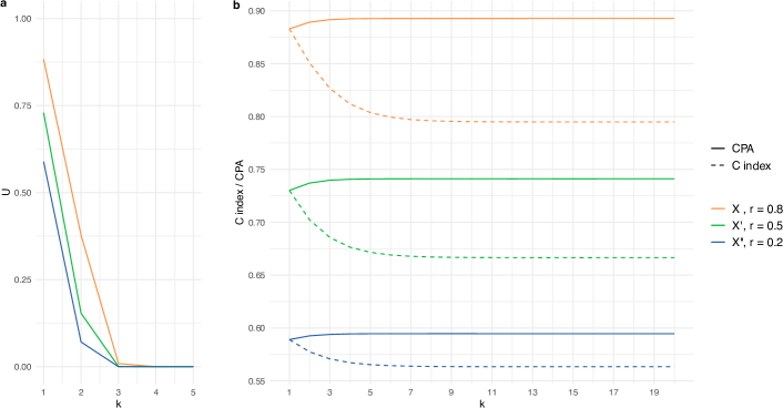
Figure 5: Rank based performance measures for the features $X$, $X^{\prime}$ and $X^{\prime\prime}$ as predictors of the real-valued outcome $Y$ in the simulation example of Section 2.3, with Pearson correlation coefficient $r=0.8$, $0.5$ and $0.2$, respectively, based on a sample of size $n=2^{20}$. We discretize the continuous outcome into $2^{k}$ consecutive blocks of size $2^{20-k}$ each, and plot (a) $U$, and (b) ${\rm CPA}$ and the C index as functions of the discretization level $k=1,\ldots,20$. Note that $k=1$ yields a binary outcome and $k=20$ a continuous outcome.

In view of the above requirements and properties, we restrict the subsequent comparison to ${\rm CPA}$, the C index, and the $U$ measure introduced by Waegeman et al. (2008). For a dataset with $m$ classes $U$ equals the proportion of sequences of $m$ instances, one of each class, that align correctly with the feature values. As noted, these measures are rank based and reduce to ${\rm AUC}$ when the outcome is binary and there are no ties in the feature values. In the continuous case with no ties in the feature values nor in the outcomes, they become symmetric, $U$ attains the value 1 under a perfect ranking and the value 0 otherwise, ${\rm C}=\frac{1}{2}\left(1-\tau_{\scriptstyle\hskip 0.56905pt\rm K}\right)$, and ${\rm CPA}=\frac{1}{2}\left(1-\rho_{\scriptstyle\rm S}\right)$.

In Fig. 5 we report on a simulation experiment where we draw samples of $2^{20}$ instances from the joint Gaussian distribution of the random vector $(Y,X,X^{\prime},X^{\prime\prime})$ with covariance matrix (6), so that the features have Pearson correlation coefficient $r=0.8$, $0.5$, and $0.2$ with the continuous outcome $Y$. By discretizing the outcome into $2^{k}$ consecutive blocks of size $2^{20-k}$ each, where $k=1,\ldots,20$, and computing ${\rm CPA}$, the C index and the $U$ measure as a function of $k$, all discretization levels are considered, ranging from a binary variable for $k=1$ to continuous outcomes for $k=20$. When $k=1$ the three measures coincide and equal ${\rm AUC}$, essentially at the population value of

$${\rm AUC}_{1/2}=\frac{2}{\pi}\arcsin\frac{r}{\sqrt{2}}+\frac{1}{2},$$ (27)

in the sense stated subsequent to (21). The $U$ measure is tailored to ordinal outcomes with a few classes only and degenerates rapidly with $k$. When $k=20$, ${\rm CPA}$ and the C index are rescaled versions of Spearman’s $\rho_{\scriptstyle\rm S}$ and Kendall’s $\tau_{\scriptstyle\hskip 0.56905pt\rm K}$, essentially at the population values in Table 1.

Throughout, the measures lie in between their common value for $k=1$, which equals ${\rm AUC}$, and the respective values for $k=20$. For all features and all $k>1$, the C index is smaller than ${\rm CPA}$, and ${\rm CPA}$ varies considerably less with the discretization level than the C index. To supplement these experiments with an analytic demonstration, suppose that $X$ and $Y$ are bivariate Gaussian with nonnegative Pearson correlation $r$. If we convert $Y$ to a balanced binary outcome, then both ${\rm CPA}$ and the C index reduce to a common value, namely, ${\rm AUC}_{1/2}$ in (27). As a function of $r$, the ratio of the C index for the continuous vs. the balanced binary outcome attains values between 0.8996 and 1, whereas for ${\rm CPA}$ the respective ratio remains between 1 and 1.0156, as illustrated in Fig. 6. These findings along with results in Capéraà and Genest (1993) and Schreyer et al (2017) suggest that, quite generally, ${\rm CPA}$ and the C index yield qualitatively similar results in practice, with ${\rm CPA}$ being less sensitive to quantization effects, and the value of ${\rm CPA}$ typically being larger than for the C index.

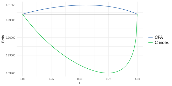
Figure 6: Ratio of ${\rm CPA}$ (blue curve) respectively the C index (green curve) for the feature $X$ as a predictor of the continuous outcome $Y$ over ${\rm AUC}$ for $X$ and the balanced binary outcome $\mathbbm{1}\{Y\geq 0\}$, where $X$ and $Y$ are bivariate Gaussian with Pearson correlation $r\in[0,1]$. The solid horizontal line is at a ratio of 1, which is attained when $r=0$ and $r=1$.

4.5 Computational issues

We turn to a discussion of the computational costs of generalized ROC analysis for a dataset of the form (8) or (14) with $n$ instances and $m\leq n$ classes.

It is well known that a traditional ROC curve can be generated from a dataset with $n$ instances in $O(n\log n)$ operations (Fawcett, 2006, Algorithm 1). A ROC movie comprises $m-1$ traditional ROC curves, so in a naïve approach, ROC movies can be computed in $O(mn\log n)$ operations. However, our implementation takes advantage of recursive relations between consecutive component curves ROC_i-1 and ROC_i. While a formal analysis will need to be left to future work, we believe that our algorithm has computational costs of $O(n\log n)$ operations only. If the number $m$ of unique values of the outcome is large, then for all practical purposes the ROC movie can be shown at a modest number $m_{0}$ of distinct values only, at a computational cost of $O(m_{0}n\log n)$ operations. For example, in the setting of Fig. 8 in the meteorological case study in Section 5.2 there are $m=35,993$ unique values of the outcome, whereas the ROC movie uses $m_{0}=401$ frames only. For the vertical averaging of the component curves in the construction of UROC curves, we partition the unit interval into 1,000 equally sized subintervals.

Importantly, ${\rm CPA}$ can be computed in $O(n\log n)$ operations, without any need to invoke ROC analysis, by sorting $x_{1},\ldots,x_{n}$ and $y_{1},\ldots,y_{n}$, computing the respective mid ranks and classes, and plugging into the rank based representation (18). Similarly, there are algorithms for the computation of the C index in $O(n\log n)$ operations (Knight, 1966; Christensen, 2005).

4.6 Key properties: Comparison to traditional ROC analysis

We are now in a position to judge whether the proposed toolbox of ROC movies, UROC curves, and ${\rm CPA}$ constitutes a proper generalization of traditional ROC analysis. To facilitate the assessment, the subsequent statements admit immediate comparison with the key insights of classical ROC analysis, as summarized in Section 2.4.

We start with the trivial but important observation that the new tools nest the notions of traditional ROC analysis. This is not to be taken for granted, as extant generalizations do not necessarily share this property.

• In the case of a binary outcome, both the ROC movie and the UROC curve reduce to the ROC curve, and ${\rm CPA}$ reduces to ${\rm AUC}$.

• ROC movies, the UROC curve and ${\rm CPA}$ are straightforward to compute and interpret, in the (rough) sense of the larger the better.

• ${\rm CPA}$ attains values between 0 and 1 and relates linearly to the covariance between the class of the outcome and the mid rank of the feature, relative to the covariance between the class and the mid rank of the outcome. In particular, if the outcomes are pairwise distinct, then ${\rm CPA}=\frac{1}{2}\left(\hskip 0.56905pt\rho_{\rm M}+1\right)$, where $\rho_{\rm M}$ is Spearman’s mid rank adjusted coefficient (25). If the outcomes are binary, then ${\rm CPA}=\frac{1}{2}\left(D+1\right)$ in terms of Somers’ $D$. For a perfect feature, ${\rm CPA}=1$, $\rho_{\rm M}=1$ under pairwise distinct and $D=1$ under binary outcomes. For a feature that is independent of the outcome, ${\rm CPA}=\frac{1}{2}$, $\rho_{\rm M}=0$ under pairwise distinct and $D=0$ under binary outcomes.

• The numerical value of ${\rm CPA}$ admits an interpretation as a weighted probability of concordance for feature–outcome pairs, with weights that grow linearly in the class based distance between outcomes.

• ROC movies, UROC curves, and ${\rm CPA}$ are purely rank based and, therefore, invariant under strictly increasing transformations. Specifically, if $\phi:\to$ and $\psi:\to$ are strictly increasing, then the ROC movie, UROC curve, and ${\rm CPA}$ computed from

  $$(\phi(x_{1}),\psi(y_{1})),\ldots,(\phi(x_{n}),\psi(y_{n}))\,\in\,\times$$ (28)

  are the same as the ROC movie, UROC curve, and ${\rm CPA}$ computed from the data in (8).

We iterate and emphasize that, as an immediate consequence of the final property, ROC movies, UROC curves, and ${\rm CPA}$ assess the discrimination ability or potential predictive ability of a point forecast, regression output, feature, marker, or test. Markedly different techniques are called for if one seeks to assess a forecast’s actual value in any given applied problem (Ben Bouallègue et al., 2015; Ehm et al., 2016).

5 Real data examples

In the following examples from survival analysis and numerical weather prediction the usage of ROC movies, UROC curves, and ${\rm CPA}$ is demonstrated. We start by returning to the survival example from Section 1, where the new set of tools frees researchers form the need to artificially binarize the outcome. Then the use of ${\rm CPA}$ is highlighted in a study of recent progress in numerical weather prediction (NWP), and in a comparison of the predictive performance of NWP models and convolutional neural networks.

5.1 Survival data from Mayo Clinic trial

In the introduction, Figs. 1 and 2 serve to illustrate and contrast traditional ROC curves, ROC movies and UROC curves. They are based on a classical dataset from a Mayo Clinic trial on primary biliary cirrhosis (PBC), a chronic fatal disease of the liver, that was conducted between 1974 and 1984 (Dickson et al., 1989). The data are provided by various R packages, such as SMPracticals and survival, and have been analyzed in textbooks (Fleming and Harrington, 1991; Davison, 2003). The outcome of interest is survival time past entry into the study. Patients were randomly assigned to either a placebo or treatment with the drug D-penicillamine. However, extant analyses do not show treatment effects (Dickson et al., 1989), and so we follow previous practice and study treatment and placebo groups jointly.

We consider two biochemical markers, namely, serum albumin and serum bilirubin concentration in mg/dl, for which higher and lower levels, respectively, are known to be indicative of earlier disease stages, thus supporting survival. Hence, for the purposes of ROC analysis we reverse the orientation of the serum bilirubin values. Given our goal of illustration, we avoid complications and remove patient records with censored survival times, to obtain a dataset with $n=161$ patient records and $m=156$ unique survival times. The proper handling of censoring is beyond the scope of our study, and we leave this task to subsequent work. For a discussion and comparison of extant approaches to handling censored data in the context of time-dependent ROC curves see Blanche et al. (2013).

The traditional ROC curves in Fig. 1 are obtained by binarizing survival time at a threshold of 1462 days, which is the survival time in the data record that gets closest to four years. The ROC movies and UROC curves in Fig. 2 are generated directly from the survival times, without any need to artificially pick a threshold. The ${\rm CPA}$ values for serum albumin and serum bilirubin are $0.73$ and $0.77$, respectively, and contrary to the ranking in Fig. 1, where bilirubin was deemed superior, based on outcomes that were artificially made binary. Our tools free researchers from the need to binarize, and still they allow for an assessment at the binary level, if desired. For example, the ROC curves and ${\rm AUC}$ values from Fig. 1 appear in the ROC movie at a threshold value of 1462 days. In line with current uses of ${\rm AUC}$ in a gamut of applied settings, ${\rm CPA}$ is particularly well suited to the purposes of feature screening and variable selection in statistical and machine learning models (Guyon and Elisseeff, 2003). Here, ${\rm AUC}$ and ${\rm CPA}$ demonstrate that both albumin and bilirubin contribute to prognostic models for survival (Dickson et al., 1989; Fleming and Harrington, 1991).

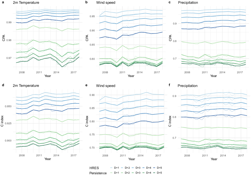
Figure 7: Temporal evolution of ${\rm CPA}$ and the C index for forecasts from the ECMWF high-resolution model at lead times of one to five days in comparison to the simplistic persistence forecast in terms of ${\rm CPA}$ (a, b, c) and the C index (d, e, f). The weather variables considered are (a, d) surface (2-meter) temperature, (b, e) surface wind speed and (c, f) 24-hour precipitation accumulation. The measures refer to a domain that covers Europe and twelve-month periods that correspond to January–December (solid and dotted lines), April–March, July–June and October–September (dotted lines only), based on gridded forecast and observational data from January 2007 through December 2018.

[label = myAnim7, height = 75mm]28figures/Test4_reduced3

Figure 8: ROC movies, UROC curves, and ${\rm CPA}$ for ECMWF high-resolution (HRES) and persistence forecasts of 24-hour precipitation accumulation over Europe at a lead time of five days in calendar year 2018. In the ROC movies, the number at upper left shows the threshold at hand in the unit of millimeter, the number at upper center the relative weight $w_{c}/\max_{l=1,\ldots,m-1}w_{l}$ from (11), and the numbers at bottom right the respective ${\rm AUC}$ values.

5.2 Monitoring progress in numerical weather prediction (NWP)

Here we illustrate the usage of ${\rm CPA}$ in the assessment of recent progress in numerical weather prediction (NWP), which has experienced tremendous advance over the past few decades (Bauer et al., 2015; Alley et al., 2019; Ben Bouallègue et al., 2019). Specifically, we consider forecasts of surface (2-meter) temperature, surface (10-meter) wind speed and 24-hour precipitation accumulation initialized at 00:00 UTC at lead times from a single day (24 hours) to five days (120 hours) ahead from the high-resolution model operated by the European Centre for Medium-Range Weather Forecasts (ECMWF Directorate, 2012), which is generally considered the leading global NWP model. The forecast data are available at https://confluence.ecmwf.int/display/TIGGE. As observational reference we take the ERA5 reanalysis product (Hersbach et al., 2018). We use forecasts and observations from $279\times 199=55,521$ model grid boxes of size $0.25^{\circ}\times 0.25^{\circ}$ each in a geographic region that covers Europe from 25.0^∘ W to 44.5^∘ E in latitude and 25.0^∘ N to 74.5^∘ N in longitude. The time period considered ranges from January 2007 to December 2018.

In Fig. 7 we apply ${\rm CPA}$ and the C index to compare forecasts from the ECMWF high-resolution run to a reference technique, namely, the persistence forecast. The persistence forecast is simply the most recent available observation for the weather quantity of interest; as such, the forecast value does not depend on the lead time. ${\rm CPA}$ and the C index are computed on rolling twelve-month periods that correspond to January–December, April–March, July–June or October–September, typically comprising $n=365\times 55,521=20,265,165$ individual forecast cases. The ECMWF forecast has considerably higher ${\rm CPA}$ and C index than the persistence forecast for all lead times and variables considered. For the persistence forecast the measures fluctuate around a constant level; for the ECMWF forecast they improve steadily, attesting to continuing progress in NWP (Bauer et al., 2015; Alley et al., 2019; Ben Bouallègue et al., 2019; Haiden et al., 2021).

To place these findings further into context, recall that ${\rm CPA}$ is a weighted average of ${\rm AUC}$ values for binarized outcomes at individual threshold values, as have been used for performance monitoring by weather centers (Ben Bouallègue et al., 2019; Haiden et al., 2021). The ${\rm CPA}$ measure preserves the spirit and power of classical ROC analysis, and frees researchers from the need to binarize real-valued outcomes. Results in terms of the C index are qualitatively similar, with the numerical value of ${\rm CPA}$ being higher than for the C index.

The ROC movies, UROC curves, and ${\rm CPA}$ values in Fig. 8 compare the ECMWF high-resolution forecast to the persistence forecast for 24-hour precipitation accumulation at a lead time of five days in calendar year 2018. As noted, this record comprises more than 20 million individual forecast cases, and there are $m=35,993$ unique values of the outcome. We certainly lack the patience to watch the full sequence of $m-1$ screens in the ROC movie. A pragmatic solution is to consider a subset ${\cal C}\subseteq\{1,\ldots,m-1\}$ of indices, so that ${\rm ROC}_{c}$ is included in the ROC movie (if and) only if $c\in{\cal C}$. Specifically, we set positive integer parameters $a\leq m-1$ and $b$ such that the ROC movie comprises at least $a$ and at most $a+b$ curves. Let the integer $s$ be defined such that $1+(a-1)s\leq m-1$ $<1+as$, and let ${\cal C}_{a}=\{1,1+s,\ldots,1+(a-1)s\}$, so that $|{\cal C}_{a}|=a$. Let ${\cal C}_{b}=\{c:n_{c}\geq n/b\}$; evidently, $|{\cal C}_{b}|\leq b$. Finally, let ${\cal C}={\cal C}_{a}\cup{\cal C}_{b}$ so that $a\leq|{\cal C}|\leq a+b$. We have made good experiences with choices of $a=400$ and $b=100$, which in Fig. 8 yield a ROC movie with 401 screens.

5.3 WeatherBench: Convolutional neural networks (CNNs) vs. NWP models

As noted, operational weather forecasts are based on the output of global NWP models that represent the physics of the atmosphere. However, the grid resolution of NWP models remains limited due to finite computing resources (Bauer et al., 2015). Spurred by the ever increasing popularity and successes of machine learning models, alternative, data-driven approaches are in vigorous development, with convolutional neural networks (CNNs; LeCun et al., 2015) being a particularly attractive starting point, due to their ease of adaptation to spatio-temporal data. Rasp et al. (2020) introduce WeatherBench, a ready-to use benchmark dataset for the comparison of data-driven approaches, such as CNNs and a classical linear regression (LR) based technique, to NWP models, such as the aforementioned HRES model and simplified versions thereof, T63 and T42, which run at successively coarser resolutions. Furthermore, WeatherBench supplies baseline methods, including both the persistence forecast and climatological forecasts.

As evaluation measure for the various types of point forecasts, WeatherBench uses the root mean squared error (RMSE). In related studies, the RMSE is accompanied by the anomaly correlation coefficient (ACC), i.e., the normalized product moment between the difference of the forecast at hand and the climatological forecast, and the difference between the outcome and the climatological forecast (Weyn et al., 2020). However, as noted by Rasp et al. (2020), results in terms of RMSE and ACC tend to be very similar. Here we argue that a rank based measure, such as ${\rm CPA}$ or the C index, would be a more suitable companion measure to RMSE than ACC.

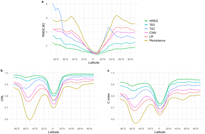
Figure 9: Predictive ability of WeatherBench three days ahead forecasts of 850 hPa temperature in 2017 and 2018 at different latitudes in terms of (a) RMSE, (b) ${\rm CPA}$, and (c) the C index. HRES, T63, and T42 indicate NWP models run at decreasing grid resolution that are compared to the CNN, linear regression (LR), and persistence forecasts (Rasp et al., 2020). Note that RMSE is negatively oriented (the smaller the better), whereas ${\rm CPA}$ and the C index are positively oriented.

Figure 9 compares WeatherBench forecasts three days ahead for temperature at 850 hPa pressure, which is at around 1.5 km height, in terms of RMSE (in Kelvin), ${\rm CPA}$, and the C index. With reference to Table 2 of Rasp et al. (2020), we consider the persistence forecast, the (direct) linear regression (LR) forecast, the (direct) CNN forecast, the Operational IFS (HRES) forecast, and successively coarser versions thereof (T63 and T42). The panels display the performance measures as functions of latitude bands, from the South Pole at 90^∘S to the equator at 0^∘ and the North Pole at 90^∘N, for the WeatherBench final evaluation period of the years 2017 and 2018. The measures are initially computed grid cell by grid cell, and then averaged across the grid cells in a latitude band, which is compatible with the latitude based weighting that is employed in WeatherBench. Note that RMSE is negatively oriented (the smaller, the better), whereas the rank based measures are positively oriented (the closer to the ideal value of 1 the better).

With respect to RMSE (Fig. 9a) marked geographical differences are visible. In equatorial regions, where day-to-day temperature variations are generally low, all forecasts have a low RMSE and the range between the best-performing HRES forecast and the simplistic persistence forecast is small. The HRES forecast remains best for all latitudes, followed by the T63 forecast. The coarsest dynamical model forecast, T42, shows a further deterioration as expected, but with large outliers in the high latitudes of the southern hemisphere and in the 30s of the northern hemisphere. It is likely that the lack of model orography creates large errors in areas of high terrain such as the Antarctic plateau and the Himalayas. Among the data-driven forecasts, CNN is better than LR for all extratropical latitudes. Finally, persistence performs worst through all latitudes with prominent peaks near 50^∘S and 50^∘N. These are the midlatitude storm track regions, where day-to-day changes are large and impede good forecasts based on persistence.

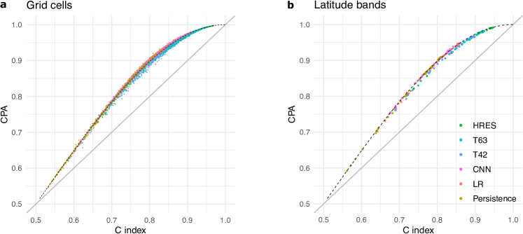
Figure 10: Comparison of ${\rm CPA}$ and the C index for WeatherBench three days ahead forecasts of 850 hPa temperature in 2017 and 2018. The points in the scatterplots of ${\rm CPA}$ vs. the C index correspond to (a) measures for individual grid cells and (b) averages of measures over latitude bands. The dashed curves show the theoretical relationship between ${\rm CPA}$ and the C index in bivariate Gaussian populations.

The corresponding results in terms of ${\rm CPA}$ and the C index (Fig. 9b–c) resemble each other, but show remarkable differences to the RMSE based analysis. Most notable are their low values in the tropics, which indicate poor performance of all forecasts, well in line with recent findings in meteorology (Kniffka et al., 2020). In contrast, the low RMSE suggests superior performance in this region. The rank based measures are independent of magnitude and thus provide a scale free assessment of predictability. Another striking difference to RMSE is the large drop in the Furious Fifties of the southern hemisphere, creating a large asymmetry with the northern midlatitudes. This area is almost entirely oceanic and characterized by mobile low-pressure systems, the dynamical behaviour of which appears to be difficult to learn under data-driven approaches.

In Fig. 10 we compare ${\rm CPA}$ and the C index, both for individual grid cells and for measures that have been averaged over latitude bands. The scatterplots illustrate the findings from Sections 4.3 and 4.4, in that the value of ${\rm CPA}$ throughout is larger than for the C index, in remarkably close agreement with the respective theoretical relationship under the assumption of bivariate Gaussianity.

We conclude that RMSE and the rank based measures bring orthogonal facets of predictive performance to researchers’ attention, and encourage the usage of of ${\rm CPA}$ or the C index to supplement RMSE as key performance measures in WeatherBench. While ACC is scale free as well, it is moment based rather than rank based, and thus is more closely aligned with RMSE than a rank based measure. Similar recommendations apply in many practical settings, where predictions of a real-valued outcome are evaluated, and a magnitude dependent measure, such as RMSE, is usefully accompanied by a rank based criterion of predictive performance. In the special case of probabilistic classifiers for binary outcomes, this corresponds to reporting both the Brier mean squared error measure and ${\rm AUC}$. See Hernández-Orallo et al. (2012) for a detailed, theoretically oriented comparison of these and other performance measures under binary outcomes.

6 Discussion

We have addressed a long-standing challenge in data analytics, by introducing a set of tools — comprising receiver operating characteristic (ROC) movies, universal ROC (UROC) curves, and a coefficient of predictive ability (${\rm CPA}$) measure — for generalized ROC analysis, thereby freeing researchers from the need to artificially binarize real-valued outcomes, which often is associated with undesirable effects (Altman and Royston, 2006). Throughout the paper, we have assumed that predictors and features are linearly ordered, thereby covering binary, ordinal, and continuous outcomes simultaneously. While our motivating example uses data from a clinical trial, our approach does not account for censored data, as typically encountered in survival analysis. We strongly encourage extensions of ROC movies, UROC curves and ${\rm CPA}$ that apply to censored data, perhaps along the lines of Blanche et al. (2013). For generalizations of ROC analysis to multi-class problems with categorical outcomes that cannot be linearly ordered see Hand and Till (2001), Ferri et al. (2003), and Section 9 of Fawcett (2006).

ROC movies, UROC curves, and ${\rm CPA}$ reduce to the classical ROC curve and ${\rm AUC}$ when applied to binary data. Moreover, attractive properties of ROC curves, such as invariance under strictly increasing transformations and straightforward interpretability are maintained by ROC movies and UROC curves. In contrast to customarily used measures of bivariate association and dependence (Reshef et al., 2011; Weihs et al., 2018), ${\rm CPA}$ is asymmetric, i.e., in general, its value changes if the roles of the feature and the outcome are transposed. However, when both the feature and the outcome are continuous, ${\rm CPA}$ becomes symmetric, and relates linearly to Spearman’s rank correlation coefficient. Thus, ${\rm CPA}$ bridges and generalizes ${\rm AUC}$, Somers’ $D$ and Spearman’s rank correlation coefficient, up to a linear relationship, just like the C index connects and generalizes ${\rm AUC}$, Somers’ $D$ and Kendall’s rank correlation coefficient. While in typical practice the two measures yield qualitatively similar results, under positive dependence ${\rm CPA}$ is larger than the C index, and ${\rm CPA}$ tends to be less affected by discretization effects.

In view of the advent of dynamic graphics in mainstream scientific publishing, we contend that ROC movies, UROC curves, and ${\rm CPA}$ are bound to supersede traditional ROC curves and ${\rm AUC}$ in a wealth of applications. Open source code for their implementation in Python (Python, 2021) and the R language and environment for statistical computing (R Core Team, 2021) is available on GitHub at https://github.com/evwalz/urocc and https://github.com/evwalz/uroc.

References

- Adams and Hands (1999) Adams, N. M., & Hands, D. J. (1999). Comparing classifiers when the misallocation costs are uncertain. Pattern Recognit. 32, 1139–1147.
- Alley et al. (2019) Alley, R. B., Emanuel, K. A., & Zhang, F. (2019). Advances in weather prediction. Science 363, 342–344.
- Altman and Royston (2006) Altman, D. G., & Royston, P. (2006). The cost of dichotomising continuous variables. Brit. Med. J. 332, 1080.
- Bauer et al. (2015) Bauer, P., Thorpe, A., & Brunet, G. (2015). The quiet revolution of numerical weather prediction. Nature 525, 47–55.
- Ben Bouallègue et al. (2015) Ben Bouallègue, Z., Pinson, P., & Friederichs, P. (2015). Quantile forecast discrimination and value. Q. J. R. Meteorol. Soc. 141, 3415–3424.
- Ben Bouallègue et al. (2019) Ben Bouallègue, Z., Magnusson, L., Haiden, T., & Richardson, D. S. (2019). Monitoring trends in ensemble forecast performance focusing on surface variables and high-impact events. Q. J. R. Meteorol. Soc. 145, 1741–1755.
- Bi and Bennett (2003) Bi, J., & Bennett, K. P. (2003). “Regression error characteristic curves”. In Proceedings of the Twentieth International Conference on Machine Learning (ICML 2003) (AAAI Press).
- Blanche et al. (2013) Blanche, P., Dartigues, J.-F., & Jacqmin-Gatta, H. (2013). Review and comparison of ROC curve estimators for a time-dependent outcome with marker-dependent censoring. Biometr. J. 55, 687–704.
- Bradley (1997) Bradley, A. P. (1997). The use of the area under the ROC curve in the evaluation of machine learning algorithms. Pattern Recognit. 30, 1145–1159.
- Capéraà and Genest (1993) Capéraà, P., & Genest, C. (1993). Spearman’s is larger than Kendall’s for positively dependent random variables. Nonparametr. Stat. 2, 183–194.
- Christensen (2005) Christensen, D. (2005). Fast algorithms for the calculation of Kendall’s . Comput. Stat. 20, 51–62.
- Davison (2003) Davison, A. C. (2003). Statistical Models (Cambridge University Press).
- Dickson et al. (1989) Dickson, E. R., Grambsch, P. M., Fleming, T. R., Fischer, L. D., & Langworthy, A. (1989). Prognosis in primary biliary cirrhosis: Model for decision making. Hepatology 10, 1–7.
- ECMWF Directorate (2012) ECMWF Directorate (2012). Describing ECMWF’s forecasts and forecasting system. ECMWF Newsl. 133, 11–13.
- Ehm et al. (2016) Ehm, W., Gneiting, T., Jordan, A., & Krüger, F. (2016). Of quantiles and expectiles: Consistent scoring functions, Choquet representations and forecast rankings (with discussion and rejoinder). J. R. Stat. Soc. Series B Stat. Methodol. 78, 505–562.
- Etzioni et al. (1999) Etzioni, R., Pepe, M., Longton, G., Hu, C., & Goodman, G. (1999). Incorporating the time dimension in receiver operating characteristic curves: A case study of prostate cancer. Med. Decis. Mak. 19, 242–251.
- Fawcett (2006) Fawcett, T. (2006). An introduction to ROC analysis. Pattern Recognit. Lett. 27, 861–874.
- Ferri et al. (2003) Ferri, C., Hernández-Orallo, J., & Salido, M. A. (2003). “Volume under the ROC surface for multi-class problems”. In Proceedings of the 14th European Conference on Machine Learning, Lavrac̆, N. et al., eds. (Springer), pp. 108–120.
- Flach (2016) Flach, P. A. (2016). “ROC analysis”. In Encyclopedia of Machine Learning and Data Mining (Springer).
- Fleming and Harrington (1991) Fleming, T. R., & Harrington, D. P. (1991). Counting Processes and Survival Analysis (Wiley).
- Gneiting and Vogel (2018) Gneiting, T., & Vogel, P. (2018). Receiver operating characteristic (ROC) curves, https://arxiv.org/abs/1809.04808.
- Guyon and Elisseeff (2003) Guyon, I., & Elisseeff, A. (2003). An introduction to variable and feature selection. J. Mach. Learn. Res. 3, 1157–1182.
- Haiden et al. (2021) Haiden, T., Janousek, M., Vitart, F., Ben Bouallegue, Z., Ferranti, L., Prates, F., & Richardson, D. (2021). Evaluation of ECMWF forecasts, including the 2020 upgrade, https://www.ecmwf.int/sites/default/files/elibrary/2021/19879-evaluation-ecmwf-forecasts-including-2020-upgrade.pdf
- Hand and Till (2001) Hand, D. J., & Till, R. J. (2001). A simple generalization of the area under the ROC curve to multiple class classification problems. Mach. Learn. 45, 171–186.
- Hanley and McNeil (1982) Hanley, J. A., & McNeil, B. J. (1982). The meaning and use of the area under a receiver operating characteristic (ROC) curve. Radiology 143, 29–36.
- Harrell et al. (1996) Harrell, F. E. Jr., Lee, K. L., & Mark, D. B. (1996). Tutorials in biostatistics: Multivariable prognostic models: Issues in developing models, evaluating assumptions and adequacy, and measuring and reducing errors. Stat. Med. 15, 361–387.
- Heagerty et al. (2000) Heagerty P. J., Lumley T., & Pepe M. S. (2000). Time-dependent ROC curves for censored survival data and a diagnostic marker. Biometrics 56, 337–344.
- Heagerty and Zheng (2005) Heagerty, P. J., & Zheng, Y. (2005). Survival model predictive accuracy and ROC curves. Biometrics 61, 92–105.
- Herbrich (2000) Herbrich, R., Graepel, T., & Obermayer, K. (2000). “Large margin rank boundaries for ordinal regression”. In Advances in Large Margin Classifiers, Smola, A. J., Bartlett, P. L., Schölkopf, B., Schuurmans, D., eds. (MIT Press), pp. 115–132.
- Hernández-Orallo (2013) Hernández-Orallo J. (2013). ROC curves for regression. Pattern Recognit. 46, 3395–3411.
- Hernández-Orallo et al. (2012) Hernández-Orallo J., Flach, P., & Ferri, C. (2012). A unified view of performance metrics: Translating threshold choice into expected classification. J. Mach. Learn. Res. 13, 2813–2869.
- Hersbach et al. (2018) Hersbach, H., Bell, B., Berrisford, P., Biavati, G., Horányi, A., Muoz Sabater, J., Nicolas, J., Peubey, C., Radu, R., Rozum, I., Schepers, D., Simmons, A., Soci, C., Dee, D., Thépaut, J.-N. (2018). ERA5 hourly data on single levels from 1979 to present. Copernicus Climate Change Service (C3S) Climate Data Store (CDS), https://doi.org/10.24381/cds.adbb2d47.
- Huang and Ling (2005) Huang, J., & Ling, C. X. (2005). Using AUC and accuracy in evaluating learning algorithms. IEEE Trans. Knowl. Data Eng. 17, 299–310.
- Kniffka et al. (2020) Kniffka, A., Knippertz, P., Fink A. H., Benedett, A., Brooks, M. E., Hill, P. G., Maranan, M., Pante, G., & Vogel, B. (2020). An evaluation of operational and research weather forecasts for southern West Africa using observations from the DACCIWA field campaign in June–July 2016. Q. J. R. Meteorol. Soc. 146, 1121–1148.
- Knight (1966) Knight, W. R. (1966). A computer method for calculating Kendall’s tau with ungrouped data. J. Am. Stat. Assoc. 61, 436–439.
- Kruskal (1958) Kruskal, W. H. (1958). Ordinal measures of association. J. Am. Stat. Assoc. 53, 814–861.
- LeCun et al. (2015) LeCun, Y., Bengio, Y., & Hinton, G. (2015). Deep learning. Nature 521, 436–444.
- Mason and Weigel (2009) Mason, S. J., & Weigel, A. P. (2009). A generic forecast verification framework for administrative purposes. Mon. Wea. Rev. 137, 331–349.
- Nešlehová (2007) Nešlehová, J. (2007). On rank correlation measures for non-continuous random variables. J. Multivar. Anal. 98, 544–567.
- Pencina and D’Agostino (2004) Pencina, M. J., & D’Agostino, R. B. (2004). Overall as a measure of discrimination in survival analysis: Model specific population value and confidence interval estimation. Stat. Med. 22, 2109–2123.
- Pepe (2003) Pepe, M. S. (2003). The Statistical Evaluation of Medical Tests for Classification and Prediction (Oxford University Press).
- Python (2021) Python Software Foundation (2021). Python language reference, http://www.python.org.
- R Core Team (2021) R Core Team (2021). R: A language and environment for statistical computing. R Foundation for Statistical Computing, Vienna, Austria, https://www.r-project.org/.
- Rasp et al. (2020) Rasp, S., Dueben, P.D., Scher, S., Weyn, J.A., Mouatadid, S., & Thuerey N. (2020). WeatherBench: A benchmark dataset for data-driven weather forecasting. J. Adv. Model. Earth Syst. 12, e2020MS002203.
- Reshef et al. (2011) Reshef, D. N., Reshef, Y. A., Finucane, H. K., Grossman, S. R., McVean, G., Turnbaugh, P. J., Lander, E. S., Mitzenmacher, M., & Sabeti, P. C. (2011). Detecting novel associations in large data sets. Science 334, 1518–1524.
- Rosset et al. (2005) Rosset, S., Perlich, C., & Zadrozny, B. (2005). “Ranking-based evaluation of regression models”. In Proceedings of the Fifth IEEE International Conference on Data Mining (ICDM’05) (IEEE).
- Schreyer et al (2017) Schreyer, M. L., Paulin, R., & Trutschnig, W. (2017). On the exact region determined by Kendall’s and Spearman’s . J. R. Stat. Soc. Series B Stat. Methodol. 79, 613–633.
- Somers (1962) Somers, R. H. (1962). A new asymmetric measure of association for ordinal variables. Am. Sociol. Rev. 27, 799–811.
- Spearman (1904) Spearman C. (1904). The proof and measurement of association between two things. Am. J. Psychol. 15, 72–101.
- Swets (1988) Swets, J. A. (1988). Measuring the accuracy of diagnostic systems. Science 240, 1285–1293.
- Waegeman et al. (2008) Waegeman, W., De Bets, B., & Boullart, L. (2008). ROC analysis in ordinary regression learning. Pattern Recognit. Lett. 29, 1–9.
- Weyn et al. (2020) Weyn, J. A., Durran, D. R., & Caruana, R. (2020). Improving data-driven global weather prediction using deep convolutional networks on a cubed sphere. J. Adv. Model. Earth Syst. 12, e2020MS002109.
- Weihs et al. (2018) Weihs, L., Drton, M., & Meinshausen, N. (2018). Symmetric rank covariances: A generalized framework for nonparametric measures of dependence. Biometrika 105, 547–562.
- Wilks (2019) Wilks, D. S. (2019). Statistical Methods in the Atmospheric Sciences, fourth edition (Elsevier).
- Woodbury (1940) Woodbury, M. A. (1940). Rank correlation when there are equal variates. Ann. Math. Stat. 11, 358–362.
- Xie (2013) Xie, Y. (2013). animation, an R package for creating animations and demonstrating statistical methods. J. Stat. Softw. 53.