Detection of Pristine Circumstellar Material of the Cassiopeia A Supernova
Bon-Chul Koo1∗, Hyun-Jeong Kim1,2, Heeyoung Oh3,4, John C. Raymond5, Sung-Chul Yoon1, Yong-Hyun Lee1,3, Daniel T. Jaffe4
1Department of Physics and Astronomy, Seoul National University, Seoul 08826, Korea
2Department of Astronomy and Space Science, Kyung Hee University,
Yongin-si, Gyeonggi-do 17104, Korea
3Korea Astronomy and Space Science Institute, Daejeon 34055, Korea
4Department of Astronomy, University of Texas at Austin, Austin, TX 78712, USA
5Harvard-Smithsonian Center for Astrophysics, 60 Garden Street, Cambridge, MA 02138, USA
Cassiopeia A is a nearby young supernova remnant that provides a unique laboratory for the study of core-collapse supernova explosions1. Cassiopeia A is known to be a Type IIb supernova from the optical spectrum of its light echo2, but the immediate progenitor of the supernova remains uncertain3. Here we report results of near-infrared, high-resolution spectroscopic observations of Cassiopeia A where we detected the pristine circumstellar material of the supernova progenitor. Our observations revealed a strong emission line of iron (Fe) from a circumstellar clump that has not yet been processed by the supernova shock wave. A comprehensive analysis of the observed spectra, together with an HST image, indicates that the majority of Fe in this unprocessed circumstellar material is in the gas phase, not depleted onto dust grains as in the general interstellar medium4. This result is consistent with a theoretical model5,6 of dust condensation in material that is heavily enriched with CNO-cycle products, supporting the idea that the clump originated near the He core of the progenitor7,8. It has been recently found that Type IIb supernovae can result from the explosion of a blue supergiant with a thin hydrogen envelope9-11, and our results support such a scenario for Cassiopeia A.
Core-collapse supernovae and their young remnants interact with the circumstellar material (CSM) ejected at the end of the progenitors’ lifetime12. By studying the physical and chemical characteristics of this material, we can learn how the progenitors stripped off their envelopes and exploded, which is crucial for understanding the nature of progenitors.
Cassiopeia A (Cas A) is a young ( yr)13 supernova remnant (SNR) where we observe the interaction of the SNR blast wave with the CSM. Its SN type is Type IIb, indicating that the progenitor had a thin H envelope at the time of explosion2. The morphology and expansion rates of the Cas A SNR suggest that it is interacting with a smooth red supergiant (RSG) wind14,15. The X-ray characteristics of the shocked ejecta knots and shocked ambient gas are also consistent with Cas A expanding into an RSG wind16,17. On the other hand, an X-ray spectral analysis indicates that there could have been a small bubble produced by a fast tenuous wind in the post-RSG stage16. Hence, it is uncertain whether the Cas A SN exploded in an RSG phase with the dense slow wind extending all the way to the stellar surface or if, instead, there was a short blue phase with a faster wind just prior to the explosion3.
A distinct component of the CSM in Cas A is the so-called “quasi-stationary floculli (QSFs)” (Fig. 1). These nebulosities or clumps are almost ‘stationary’ ( km s-1) and are bright in H and [N ii]6548, 6583 emission line images18-22. Their optical and near-infrared (NIR) spectra indicate that QSFs are dense (3–) and He and N enriched7,23-25. QSFs are probably dense CNO-processed circumstellar clumps that have been shocked recently by the SN blast wave14,26. It was pointed out that a progenitor of 15–25 must have lost of its mass prior to the ejection of such N-rich QSFs8, but the evolutionary stage of the progenitor and the mass loss mechanism are uncertain. It had been suggested that QSFs are the fragments of an RSG shell formed by a fast wind in the progenitor’s Wolf-Rayet phase27, but hydrodynamic simulations showed that QSFs are not consistent with such fragments15. Another suggestion was that QSFs are the clumps of an inhomogeneous RSG wind14, but it is not clear how the He- and N-rich clumps ejected from the bottom of H envelope can be at their current locations.
We report results of high-resolution, NIR spectroscopic observations of one of QSFs in Cas A where we detected the emission from unshocked, pristine CSM. The emission from shock-processed CSM in QSFs has been observed since the 1950s7,18,21-25, but the emission from the unprocessed CSM that retains the original physical and chemical conditions of the deep interior of the progenitor has never been observed. There have been observations of patchy optical emission outside the SNR that could be also an unprocessed CSM, but from the outer envelope of the progenitor ejected during the RSG phase14,28. The knot (hereafter ‘Knot 24’29) that we observed lies near the southern radio boundary of the SNR, at the tip of a prominent arc of QSFs (Fig. 1), and has been visible at least since 195120,21. The observations were performed with the Immersion GRating INfrared Spectrometer (IGRINS) mounted on the 4.3m Discovery Channel Telescope (DCT) at Lowell Observatory in 2018 December.
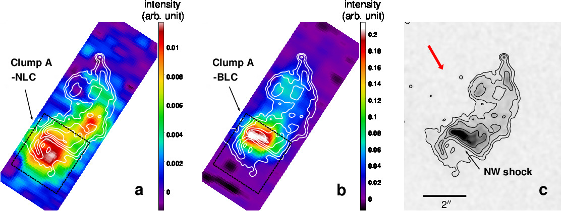
We detected a strong [Fe ii] 1.644 m line with a remarkable profile showing a very narrow line superposed on a very broad one (Fig. 2a). The broad-line component (hereafter ‘BLC’) has a velocity width of km s-1, indicating that it is emitted from shocked gas. The width of the narrow-line component (hereafter ‘NLC’) is km s-1. (See Methods and Supplementary Table 1 for the line parameters.) The entire knot revealed in the NLC map extends NW-SE and has a complex morphology with several clumps including ‘Clump A-NLC’, the largest one in the southeast (Fig. 3a). The northwestern boundary of Clump A-NLC touches and lies immediately to the southeast of a bright emission feature in the BLC map labelled ‘Clump A-BLC’ (Fig. 3b). The detailed structure of Clump A-BLC can be seen in the HST F625W image in Fig. 3c, which is dominated by the H and [N ii]6548, 6583 lines from radiative shock. The prominent emission feature in the middle of the HST image is spatially coincident with Clump A-BLC and shows a sharp decrease of brightness towards Clump A-NLC. This morphology suggests that a strong shock (hereafter the ‘NW shock’) is currently propagating into Clump A from NW to SE and that Clump A-NLC is the unshocked part of the clump. We can also see faint H+[N ii] emission along the NE rim of Clump A-NLC, implying another, weaker, shock propagating into the clump from NE to SW. There are other emission features in the NLC and BLC maps to the northwest of Clump A, but the [Fe ii] emission is faint and the relation between the narrow- and broad-line components is unclear.
We detected other [Fe ii] lines at 1.534, 1.600, and 1.677 m and the hydrogen Br line toward Clump A (Fig. 2). The electron density of Clump A-NLC inferred from the ratio of [Fe ii] lines is cm-3, which is more than an order of magnitude lower than that of the BLC ( cm-3; Supplementary Table 1). Another way to estimate the density of Clump A-NLC is to consider pressure equilibrium. Since the typical temperature of the [Fe ii]-line emitting post-shock cooling layer is K and the ionization fraction is (ref.30), the pressure of the shocked gas becomes cm-3 K. The ram pressure of the preshock gas should be comparable to this; the preshock density therefore would be cm-3. The temperature of Clump A-NLC inferred from the line widths of the Br ( km s-1) and [Fe ii] 1.644 m ( km s-1) lines is K (Methods). An order of magnitude lower density in the NLC than in the shocked gas and the estimated temperature of K, together with the morphology in Fig. 3, indicate that Clump A-NLC is unshocked, pristine CSM photoionized by UV radiation from the NW shock propagating into the clump.
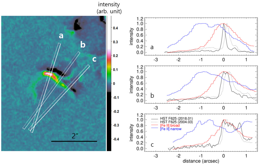
The narrow [Fe ii] 1.644 m line detected toward Clump A-NLC is strong, with the ratio of Br to [Fe ii] 1.644 m fluxes () of . This ratio is much smaller than that seen toward nebulae where Fe is believed to be heavily depleted on dust grains (e.g., 7–10 in the Orion bar31), suggesting that Fe in Clump A-NLC is mostly in the gas phase. We have analyzed the observed line ratios toward Clump A using a shock model (Methods). The analysis shows that the observed ratio of the NLC to BLC [Fe ii] 1.644 m line flux () is consistent with a shock speed of 100–125 km s-1, which agrees with the shock speed implied by the line width of the BLC ( km s-1) as well as the shock speed of the NW shock front obtained by comparing the 2018 HST image to another HST image taken in 2004 March (100–150 km s-1; Supplementary Fig. 1). While the calculated ratio that assumed solar abundance agrees with the observed ratio for the BLC, it is times the observed ratio for the NLC. The simplest interpretation, therefore, is that, in the unshocked CSM, the Fe abundance relative to H by number is 60% of solar, while, in the shocked gas, it is equal to solar, presumably because Fe locked up in dust grains is released by the shock destruction of the grains. A CSM with the majority of Fe in the gas phase is in sharp contrast to the general interstellar medium where % of Fe is in the gas phase4.
The ‘non-depletion’ of Fe in Knot 24 must reflect the physical and chemical conditions of the stellar material ejected from the progenitor in the pre-SN stage. The N and He overabundance in QSFs indicates that the QSFs originated from a N-rich layer at the bottom of the H envelope of an RSG (Fig. 4)7,8. Knot 24 is as N enriched as other QSFs; its [N ii] /H () is close to the mean value for QSFs (3.3; ref.22). Hence, Knot 24 might have originated with the other QSFs from the same N-rich layer. Note that QSFs are He overabundant relative to H by a factor of 4–10 (ref.7), suggesting that they originated near the He core where the material is heavily enriched with CNO products as in the surface of WNL stars7,8. In that thin layer, the abundances of C and O drop considerably below their solar values, while the abundances of heavier refractory elements (e.g., Mg, Si, and Fe) remain essentially the same. The composition of dust formed from such CNO-processed material would be different from that of dust formed in the outer envelope of RSG winds because neither the oxygen rich minerals of M stars nor the mixture of carbon dust and carbides as in C stars can be formed6. Theoretical model calculations found that the composition of dust formed in such material is dominated by solid Fe and FeSi alloys and that, as a consequence of the low probability of Fe grain formation, as much as 80–85% of Fe is left in the gas phase5,6,32. Hence, the non-depletion of Fe in Knot 24 is consistent with dust condensation in a CSM heavily enriched with CNO products.
When did the mass loss that ejected the QSFs occur and what was the evolutionary stage of the progenitor at that time? Proper motion studies of QSFs in Cas A found a systemic “expanding” motion with a characteristic time of ( yr and an expansion velocity of 180 km s-1 (when scaled to 3.4 kpc)19,20. If the apparent expanding motion is partly due to shock motion ( km s-1), the systemic expansion velocity could have been overestimated by a factor of . The corresponding radius and the surface temperature of the progenitor should be about 100 and K, respectively, if the progenitor mass at that stage were about 5 (Methods). These values, together with the He and N overabundance of QSFs, imply that the immediate progenitor of Cas A SN was likely a blue supergiant (BSG) with a WNL-like surface chemical composition rather than an RSG. If the expansion velocity of QSFs is lower than 100 km s-1, a yellow supergiant could be also possible. The optical spectrum of Cas A SN implies that the H envelope mass in the Cas A SN progenitor was comparable to that of SN 1993J (i.e., ; ref.2). Although the SN 1993J progenitor was identified as an RSG33, recent theoretical and observational studies indicate that both RSG and BSG solutions for Type IIb SN progenitors can be found with , for which the surface abundances are similar to WNL stars9-11. Therefore, the scenario in which the He- and N-rich, Fe-non-depleted, QSFs originated from a BSG wind emitted from the progenitor is consistent with recent theoretical and observational findings. The formation and dynamical evolution of such dense clumps in this scenario need to be explored.
References
1. Milisavljevic, D. & Fesen, R. A. The supernova - supernova remnant connection. In Alsabti, A. W. & Murdin, P. (eds.) Handbook of Supernovae, 2211-2231 (Springer International Publishing AG, 2017).
2. Krause, O. et al. The Cassiopeia A supernova was of Type IIb. Science 320, 1195-1197 (2008).
3. Chevalier, R. A. & Soderberg, A. M. Type IIb supernovae with compact and extended progenitors. Astrophys. J. Lett. 711, L40-L43 (2010).
4. Savage, B. D. & Sembach, K. R. Interstellar abundances from absorption-line observations with the Hubble space telescope. Annu. Rev. Astron. Astr. 34, 279-330 (1996).
5. Gail, H. P., Duschl, W. J., Ferrarotti, A. S. & Weis, K. Dust formation in LBV envelopes. In Humphreys, R. & Stanek, K. (eds.) The Fate of the Most Massive Stars, vol. 332 of Astronomical Society of the Pacific Conference Series, 317-319 (Astronomical Society of the Pacific, San Francisco, 2005).
6. Gail, H. P. Formation and evolution of minerals in accretion disks and stellar outflows. In Henning, T. (ed.) Astromineralogy, vol. 815, 61-141 (Springer, Berlin, 2010).
7. Chevalier, R. A. & Kirshner, R. P. Spectra of Cassiopeia A. II. Interpretation. Astrophys. J. 219, 931-941 (1978).
8. Lamb, S. A. The Cassiopeia A progenitor: a consistent evolutionary picture involving supergiant mass loss. Astrophys. J. 220, 186-192 (1978).
9. Meynet, G. et al. Impact of mass-loss on the evolution and pre-supernova properties of red supergiants. Astron. Astrophys. 575, A60 (2015).
10. Yoon, S.-C., Dessart, L. & Clocchiatti, A. Type Ib and IIb supernova progenitors in interacting binary systems. Astrophys. J. 840, 10 (2017).
11. Kilpatrick, C. D. et al. On the progenitor of the Type IIb supernova 2016gkg. Mon. Not. R. Astron. Soc. 465, 4650-4657 (2017).
12. Smith, N. Mass loss: its effect on the evolution and fate of high-mass stars. Annu. Rev. Astron. Astr. 52, 487-528 (2014).
13. Thorstensen, J. R., Fesen, R. A. & van den Bergh, S. The expansion center and dynamical age of the galactic supernova remnant Cassiopeia A. Astron. J. 122, 297-307 (2001).
14. Chevalier, R. A. & Oishi, J. Cassiopeia A and its clumpy presupernova wind. Astrophys. J. Lett. 593, L23-L26 (2003).
15. van Veelen, B., Langer, N., Vink, J., García-Segura, G. & van Marle, A. J. The hydrodynamics of the supernova remnant Cassiopeia A. The influence of the progenitor evolution on the velocity structure and clumping. Astron. Astrophys. 503, 495-503 (2009).
16. Hwang, U. & Laming, J. M. The circumstellar medium of Cassiopeia A inferred from the outer ejecta knot properties. Astrophys. J. 703, 883-893 (2009).
17. Lee, J.-J., Park, S., Hughes, J. P. & Slane, P. O. X-Ray observation of the shocked red supergiant wind of Cassiopeia A. Astrophys. J. 789, 7 (2014).
18. Baade, W. & Minkowski, R. Identification of the radio sources in Cassiopeia, Cygnus A, and Puppis A. Astrophys. J. 119, 206-214 (1954).
19. Kamper, K. & van den Bergh, S. Optical studies of Cassiopeia A. V. A definitive study of proper motions. Astrophys. J. Suppl. S. 32, 351-366 (1976).
20. van den Bergh, S. & Kamper, K. Optical studies of Cassiopeia A. VII. Recent observations of the structure and evolution of the nebulosity. Astrophys. J. 293, 537-541 (1985).
21. Lawrence, S. S. et al. Three-dimensional Fabry-Perot imaging spectroscopy of the Crab nebula, Cassiopeia A, and nova GK Persei. Astron. J. 109, 2635-2893 (1995).
22. Alarie, A., Bilodeau, A. & Drissen, L. A hyperspectral view of Cassiopeia A. Mon. Not. R. Astron. Soc. 441, 2996-3008 (2014).
23. Hurford, A. P. & Fesen, R. A. Reddening measurements and physical conditions for Cassiopeia A from optical and near-infrared spectra. Astrophys. J. 469, 246-254 (1996).
24. Gerardy, C. L. & Fesen, R. A. Near-infrared spectroscopy of the Cassiopeia A and Kepler supernova remnants. Astron. J. 121, 2781-2791 (2001).
25. Lee, Y.-H., Koo, B.-C., Moon, D.-S., Burton, M. G. & Lee, J.-J. Near-infrared knots and dense Fe ejecta in the Cassiopeia A supernova remnant. Astrophys. J. 837, 118 (2017).
26. McKee, C. F. & Cowie, L. L. The interaction between the blast wave of a supernova remnant and interstellar clouds. Astrophys. J. 195, 715-725 (1975).
27. Chevalier, R. A. & Liang, E. P. The interaction of supernovae with circumstellar bubbles. Astrophys. J. 344, 332-340 (1989).
28. Fesen, R. A., Becker, R. H. & Blair, W. P. Discovery of fast-moving nitrogen-rich ejecta in the supernova remnant Cassiopeia A. Astrophys. J. 313, 378-388 (1987).
29. Koo, B.-C. et al. A deep near-infrared [Fe II]+[Si I] emission line image of the supernova remnant Cassiopeia A. Astrophys. J. 866, 139 (2018).
30. Koo, B.-C., Raymond, J. C. & Kim, H.-J. Infrared [Fe II] emission lines from radiative atomic shocks. J. Kor. Astron. Soc. 49, 109-122 (2016).
31. Walmsley, C. M., Natta, A., Oliva, E. & Testi, L. The structure of the Orion bar. Astron. Astrophys. 364, 301-317 (2000).
32. Morris, P. W. et al. Carinae’s dusty homunculus nebula from near-infrared to submillimeter wavelengths: mass, composition, and evidence for fading opacity. Astrophys. J. 842, 79 (2017).
33. Aldering, G., Humphreys, R. M. & Richmond, M. SN 1993J: the optical properties of its progenitor. Astron. J. 107, 662-672 (1994).
34 Reed, J. E., Hester, J. J., Fabian, A. C. & Winkler, P. F. The three-dimensional structure of the Cassiopeia A supernova remnant. I. The spherical shell. Astrophys. J. 440, 706-721 (1995).
35. Paxton, B. et al. Modules for experiments in stellar astrophysics (MESA). Astrophys. J. Suppl. S. 192, 3 (2011).
Correspondence
Correspondence and requests for materials should be addressed to B.-C. K. (email: koo@astro.snu.ac.kr).
Acknowledgements
We wish to thank Rob Fesen for his helpful comments on an earlier version of the manuscript.
This research was supported by Basic Science Research Program through the National Research Foundation of Korea(NRF) funded by the Ministry of Science, ICT and future Planning (2017R1A2A2A05001337).
This work used the Immersion Grating Infrared Spectrometer (IGRINS) that was developed under a collaboration between the University of Texas at Austin and the Korea Astronomy and Space Science Institute (KASI) with the financial support of the US National Science Foundation under grant AST-1229522, of the University of Texas at Austin, and of the Korean GMT Project of KASI.
These results made use of the Discovery Channel Telescope at Lowell Observatory. Lowell is a private, non-profit institution dedicated to astrophysical research and public appreciation of astronomy and operates the DCT in partnership with Boston University, the University of Maryland, the University of Toledo, Northern Arizona University and Yale University.
Author Contributions
All authors contributed to different aspects of the project, and read and commented on the manuscript.
B.-C.K. led the project, analysis and discussion, and wrote the manuscript.
H.-J.K. performed the observation and data reduction, and contributed to the data analysis and manuscript writing.
H.O. performed the observation and contributed to the IGRINS data analysis.
J.C.R. contributed to the shock emission analysis and scientific interpretation.
S.-C.Y. contributed to the scientific interpretation and the manuscript writing.
Y.-H.L. contributed to the HST data analysis.
D.T.J. contributed to the project setup.
Competing Interests
The authors declare that they have no competing financial interests.

Methods
Observations and Data Reduction. We obtained a high-resolution, NIR spectral map of Knot 24 using the Immersion GRating INfrared Spectrometer (IGRINS)36-38 mounted on the 4.3m Discovery Channel Telescope (DCT) at Lowell Observatory on 2018 December 25 (UT). IGRINS simultaneously covers the H (1.47–1.81 m) and K (1.95–2.48 m) bands with a spectral resolving power of , corresponding to a velocity resolution of 7–8 km s-1. The slit size is . We observed five adjacent slit positions with an offset of in the slit-width direction to make a spectral map of covering the bright part of Knot 24 (Fig. 1). The position angle was 147∘, and the total on-source integration time varied from 15 min to 50 min depending on the slit position. The seeing in K-band measured from the IGRINS slit-view camera images was –. Between the on-source observations, sky frames were obtained at a position east of the on-source position for sky subtraction and wavelength calibration. We also observed the A0V-type star HR 9019 for telluric correction and flux calibration.
Data reduction was carried out with the IGRINS Pipeline Package (PLP)39 v2.2.0,
which performs sky subtraction, flat-fielding, bad-pixel correction, aperture extraction,
and wavelength calibration.
The PLP provides the 2D spectra of H and K bands with the 2D variance maps
given by Poisson noise combined with the standard deviation of the frame produced by
subtracting the off-source (sky) frames from the on-source frames.
The wavelength solution is derived by fitting OH emission lines from
the sky frames and has a typical uncertainty smaller than km s-1.
The PLP products were additionally processed by using the Plotspec
python code designed for analyzing the reduced 2D IGRINS spectra40.
Plotspec performs telluric correction, relative flux calibration, and continuum subtraction
and provides a single 2D spectrum with all orders in H- and K-bands combined.
Using Plotspec, we obtained 2D position-velocity diagrams of the observed lines for each slit
and a 3D datacube, which were used to generate average spectra and
integrated intensity maps, respectively (Figs. 2 and 3).
In Fig. 3, the NLC map was produced by subtracting a baseline over the central
velocity channels from the individual spectra, and the BLC map was obtained by
subtracting the NLC map from the total integrated intensity map.
Derivation of Line Parameters. We derived the [Fe ii] 1.644 m line parameters of the NLC by fitting the observed spectra with a Gaussian profile and those of the BLC by a direct method after subtracting the narrow Gaussian component, i.e., the line flux from a direct sum, the central velocity from an intensity-weighted average, and the velocity width by dividing the line flux by the intensity at . The parameters of Clump A were derived from the spectra extracted from the boxed area in Fig. 3. We find that Clump A contributes about 65% (62%) to the total narrow (broad) [Fe ii] 1.644 m line flux of the entire knot. The derived line parameters are summarized in Supplementary Table 1.
The other detected [Fe ii] lines at 1.534, 1.600, and 1.677 m have comparable critical densities of a few cm-3, and their ratios to the [Fe ii] 1.644 m line can be used as a density tracer. Since these lines are so weak that the NLC is barely visible in the individual spectra, we have added them to increase the signal-to-noise ratio. The resulting “[Fe ii] 1.534+” spectrum of the entire knot is shown in Fig. 2b in which we can clearly see both NLC and BLC. The ratios are 0.17 and 0.46 for the NLC and BLC, respectively (Supplementary Table 1). For Clump A, the NLC of [Fe ii] 1.534+ line is relatively weak (Fig. 2b) with an ratio of 0.12. For the BLC, the ratio is 0.54. Supplementary Table 1 lists the electron densities derived from the ratios. For the BLC, it is (1.2–1.8) cm-3. For the NLC, the derived electron densities have large uncertainties, i.e., cm-3 (entire knot) and cm-3 (Clump A). The result is not sensitive to and we assumed K.
The H Br line is very faint and can be seen only in Clump A (Supplementary Fig. 2).
In the average Br spectrum of Clump A (Fig. 2c), the NLC is clearly seen
with the line width significantly broader than the [Fe ii] 1.644 m line (Fig. 2a).
The BLC also appears to be present, but
the baseline fluctuation hampers an accurate measurement of the line parameters.
The parameters of the Br line of Clump A were obtained by
Gaussian fitting (for narrow line) and by the direct method (for broad line),
and they are listed in Supplementary Table 2.
To derive the ratio of the Br line to [Fe ii] 1.644 m line fluxes, we need to
consider the difference in extinction at two wavelengths.
Estimates of the H column density to Knot 24 indicate that
cm-2, corresponding
to mag (ref.29).
If we use the dust opacity model of the general interstellar medium41,
mag and mag, so that
the difference in the extinction at the two wavelengths is 0.5 mag, and
we divided the observed ratio by 1.6. The resulting ratios are
and for the NLC and BLC, respectively
(Supplementary Table 2). The latter, however, has a large uncertainty
due to the baseline fluctuation.
Temperature and Non-thermal Motion of Clump A. The line width (FWHM) of the narrow Br line is km s-1, much greater than that ( km s-1) of the narrow [Fe ii] 1.644 m line (Supplementary Tables 1 and 2). These widths are corrected for the instrumental broadening ( km s-1). Note that the observed FWHM of the narrow [Fe ii] 1.644 m line before the correction is 12 km s-1, which is significantly greater than the instrumental resolution. Hence, the [Fe ii] 1.644 m line is resolved, and its width is considerably greater than the thermal width ( km s-1) expected from the width of the Br line, indicating that the line broadening is due to both thermal and temperature-independent non-thermal motions. We derived the temperature and non-thermal velocity dispersion of Clump A-NLC from the velocity widths of the narrow Br and [Fe ii] 1.644 m lines, assuming that the two lines originated in the regions of similar physical conditions. The observed velocity dispersions () are related to the thermal () and non-thermal () velocity dispersions by
| (1) |
where the thermal velocity dispersions of Br and [Fe ii] 1.644 m lines are given by
| (2) |
respectively. In this equation, . The observed velocity
dispersions of the Br and [Fe ii] 1.644 m lines of Clump A-NLC are
km s-1 and
km s-1, respectively
(Supplementary Tables 1 and 2). Then, from equations (1) and (2), we obtained
km s-1 and K.
Shock Emission Analysis. We compare the observed line flux ratios with the results from a shock model where the BLC is emitted from the shocked gas, while the NLC is emitted from the ‘radiative precursor’, i.e., the region in front of the shock front heated/ionized by shock radiation. We calculated the [Fe ii] 1.644 m and Br line fluxes of the radiative precursor using the results in the MAPPINGS III Library of Fast Shock Models42. The authors provide online tables summarizing the physical structure of the precursor and shock, i.e., temperature, density, and fraction of elements in different ionization stages as a function of distance from the shock front, for a range of shock parameters. We calculated the line emissivities using these tables with updated atomic parameters and integrated the emissivities to obtain line fluxes from the precursor region.
For the atomic parameters of [Fe ii] forbidden lines, we used the effective collision strengths of ref.43 and the radiative transition probabilities ( values) of ref.44. We note that the [Fe ii] 1.644 m line fluxes in the MAPPINGS III Library can be reproduced by using the effective collision strengths and the values of refs.45,46, and they are a factor of smaller than ours. The discrepancy mainly originates from the different collisional excitation rates. The [Fe ii] atomic rates are still uncertain, but the main difference between the two sets of the collisional excitation rates is that ref.43 includes the contribution of resonances to the excitation cross sections, and they dominate the total rates for most of the forbidden transitions. In ref.30, we discussed recent updates. Note that the relative Fe abundance of two media, i.e., the unshocked and shocked CSM, depends only weakly on the adopted atomic parameters. Also, we adopted an Fe abundance of in number47, which is 1.5 times greater than that adopted in the online table. Because of these differences in parameters, our [Fe ii] 1.644 m line fluxes are a factor of greater than those in the MAPPINGS III Library. For the Br line, we computed the flux of H line with the on-the-spot approximation and multiplied by 0.033 to derive the flux of Br line, where the factor “0.033” is the ratio of the two line fluxes at K and cm-3 (ref.48). The results agree with those of the library to within a few percent.
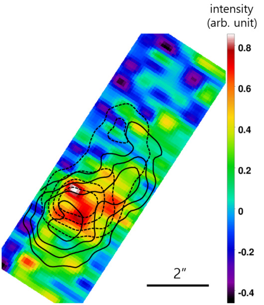
Supplementary Fig. 3a shows the physical structure of the precursor of a plane-parallel shock propagating at 125 km s-1. The preshock density is cm-3 and magnetic field strength is 0.1 G. The abscissa is H-nucleus column density from the shock front (). We see that the photoionized precursor extends to cm-2. In this precursor region, the temperature is constant at 5,500 K and H is almost fully ionized. (The H ionization fraction closely follows the Br line emissivity curve and is not shown.) The fraction of Fe in Fe+ is 0.2 at the shock front and smoothly increases to 1 in the ambient medium. Near the shock front, Fe is mostly in Fe++. Also shown are the normalized emissivities of [Fe ii] 1.644 m and Br lines. The two lines are both emitted from the entire precursor region, but the [Fe ii] 1.644 m line emissivity attains a maximum further upstream because of the variation of the Fe+ fraction. The structures of the precursors for other shock velocities are similar but with different spatial extents, e.g., cm-2 and cm-2 for 100 km s-1 and 150 km s-1 shocks. It is worthwhile to note that, in Clump A, the distribution of the Br emission is slightly offset from that of Clump A-NLC in [Fe ii] 1.644 m line (Supplementary Fig. 2), which appears consistent with this difference seen in the model.
The column density of Clump A is cm-2 where and we used pc. If cm-3, cm-2 and it is less than the total column density of the radiative precursor of the 125 km s-1 shock in Supplementary Fig. 3a. In order to compare the result of the shock model to our observations, therefore, the precursor needs to be truncated. The [Fe ii] 1.644 m line flux of such a truncated precursor can be obtained by integrating the emissivity from the shock front to a given , i.e.,
| (3) |
where is the volume emissivity of [Fe ii] 1.644 m line at , and is the distance corresponding to . This is the flux normal to the shock front, but since we will be comparing the flux ratios, its absolute value is not relevant. Supplementary Fig. 3b shows the variation of the ratio for 100, 125, and 150 km s-1 shocks. The [Fe ii] 1.644 m line flux from the shock () is obtained by scaling the result in the MAPPINGS III library because we only need the total flux. The observed flux ratio of the NLC to the BLC is 12%, which agrees with the ratio of the 100–125 km s-1 shock for – cm-2. The shock speed could be little higher depending on the density of Clump A.
We also calculated the flux ratio of Br to [Fe ii] 1.644 m lines ()
in the truncated precursor, and the result is shown in
Supplementary Fig. 3c.
The observed ratio () is slightly
larger than the ratio of the 100–125 km s-1 shock (),
but consistent within a factor of 2.
For comparison, the observed ratio
of the BLC () agrees with the ratio of shock emission predicted
from the model, e.g., 0.017 for the 125 km s-1 shock from the result
in the MAPPINGS III library.
In other words, the observed ratio is comparable to
the ratio expected for the solar abundance material in both
shocked and unshocked CSM, implying that Fe is not significantly depleted
in both media. According to the shock model presented here,
the Fe abundance relative to H by number
in the unshocked CSM is 60% of solar.
There is some additional uncertainty in this fraction
associated with atomic parameters.
Note that if % of Fe is in the gas phase as in the general interstellar
medium4, the ratio of the precursor predicted
from our shock model would be , which is an order of magnitude
greater than the observed ratio.
We also note that, since the relative ratio in
the two regions depends only weakly on the adopted [Fe ii]-line atomic parameters,
the result that Fe in the unshocked CSM is not depleted more than
a factor of than in the shocked CSM should be robust.
Estimate of the Radius and Surface Temperature of the Cas A Progenitor. Given that the stellar wind velocity should be comparable to the escape velocity from the surface of the star (i.e., ), the progenitor radius can be given by
| (4) |
The wind velocity of 100–200 inferred from the QSF proper motion implies –, if the mass of the progenitor at the final evolutionary stage was about 5 (ref.17). The stellar evolution models10 predict that the luminosity of a Type IIb SN progenitor of would be about during the final evolution. From the blackbody approximation of , we get the surface temperature –. This temperature range corresponds to a BSG. If the wind velocity is lower than 100 km s-1, the temperature could fall into the range of a yellow supergiant, e.g., 4,800–7,500 K (ref.49). The inferred surface temperature depends only weakly on the assumed progenitor mass. For example, for , we get –, and using (ref.10), –.
Data Availability
The data that support the plots within this paper and other findings of this study are
available from the corresponding author upon reasonable request.
References only in Methods
36. Yuk, I.-S. et al. Preliminary design of IGRINS (Immersion GRating INfrared Spectrograph). In McLean, I. S., Ramsay, S. K. & Takami, H. (eds.) Ground-based and Airborne Instrumentation for Astronomy III, vol. 7735 of Proceedings of SPIE, 77351M (SPIE, Washington, 2010).
37. Park, C. et al. Design and early performance of IGRINS (Immersion Grating Infrared Spectrometer). In Ramsay, S. K., McLean, I. S. & Takami, H. (eds.) Ground-based and Airborne Instrumentation for Astronomy V, vol. 9147 of Proceedings of SPIE, 91471D (SPIE, Washing- ton, 2014).
38. Mace, G. et al. IGRINS at the Discovery Channel Telescope and Gemini South. In Evans, C. J., Simard, L. & Takami, H. (eds.) Ground-based and Airborne Instrumentation for Astronomy VII, vol. 10702 of Proceedings of SPIE, 107020Q (SPIE, Washington, 2018).
39. Lee, J.-J., Gullikson, K. & Kaplan, K. F. IGRINS pipeline package (IGRINS/PLP) v2.2.0.
http://doi.org/10.5281/zenodo.845059 (2017).
40. Kaplan, K. F. et al. Excitation of molecular hydrogen in the Orion bar photodissociation region from a deep near-infrared IGRINS spectrum. Astrophys. J. 838, 152 (2017).
41. Draine, B. T. Scattering by interstellar dust grains. I. Optical and ultraviolet. Astrophys. J. 598, 1017-1025 (2003).
42. Allen, M. G., Groves, B. A., Dopita, M. A., Sutherland, R. S. & Kewley, L. J. The MAPPINGS III library of fast radiative shock models. Astrophys. J. Suppl. S. 178, 20-55 (2008).
43. Ramsbottom, C. A., Hudson, C. E., Norrington, P. H. & Scott, M. P. Electron-impact excitation of Fe II. Collision strengths and effective collision strengths for low-lying fine-structure forbidden transitions. Astron. Astrophys. 475, 765-769 (2007).
44. Deb, N. C. & Hibbert, A. Radiative transition rates for the forbidden lines in Fe II. Astron. Astrophys. 536, A74 (2011).
45. Nussbaumer, H. & Storey, P. J. Atomic data for Fe II. Astron. Astrophys. 89, 308-313 (1980).
46. Nussbaumer, H. & Storey, P. J. Transition probabilities for Fe II infrared lines. Astron. Astrophys. 193, 327-333 (1988).
47. Asplund, M., Grevesse, N., Sauval, A. J. & Scott, P. The chemical composition of the Sun. Annu. Rev. Astron. Astr. 47, 481-522 (2009).
48. Draine, B. T. Physics of the Interstellar and Intergalactic Medium (Princeton University Press, New Jersey, 2011).
49. Drout, M. R., Massey, P., Meynet, G., Tokarz, S. & Caldwell, N. Yellow supergiants in the Andromeda galaxy (M31). Astrophys. J. 703, 441-460 (2009).
SUPPLEMENTARY INFORMATION
This section contains all the supplementary data (2 tables and 3 figures) supporting the analysis presented in the main paper and the Method section.
| Entire knot | Clump A | ||
| narrow line | (km s-1) | 49.68(0.31) | 49.28(0.31) |
| (km s-1) | 7.45(0.44) | 8.45(0.47) | |
| 10.92(0.25) | 7.15(0.20) | ||
| 1.86(0.38) | 0.87(0.29) | ||
| 0.171(0.035) | 0.122(0.040) | ||
| ( cm-3) | 1.97(0.70, 0.80) | 1.05(0.64, 0.75) | |
| broad line | (km s-1) | 56.1 | 57.5 |
| (km s-1) | 205 | 189 | |
| 100 | 62.3(0.7) | ||
| 46.2(2.0) | 33.9(1.5) | ||
| 0.462(0.021) | 0.543(0.025) | ||
| ( cm-3) | 1.23(0.12, 0.13) | 1.81(0.20, 0.22) | |
| narrow to broad line ratio | 0.109(0.003) | 0.115(0.003) | |
| Note— = velocity center and velocity width of [Fe ii] 1.644 m line; =[Fe ii] 1.644 m line flux; = sum of [Fe ii] 1.534, 1.600, and 1.677 m line fluxes; = electron density derived from assuming K. The line fluxes are normalized to the [Fe ii] 1.644 m flux (= 100) of the broad line of the entire knot. For the narrow line, the line parameters are derived from a Gaussian fit and is the FWHM corrected for the instrumental broadening ( km s-1). The errors are errors. For the broad line, is the intensity weighted mean velocity and is the velocity width obtained by dividing the line flux by the intensity at . | |||
| parameter | value | |
| narrow line | (km s-1) | 51.4(1.9) |
| (km s-1) | 23.2(4.8) | |
| 1.19(0.30) | ||
| 0.104(0.026) | ||
| broad line | 1.89(0.52) | |
| 0.020(0.010) | ||
| These are extinction-corrected flux ratios (see Methods). | ||
| Note— = velocity center and velocity width; = Br line flux normalized to the [Fe ii] 1.644 m flux (= 100) of the broad line of the entire knot as in Supplementary Table 1. The velocity width is corrected for the instrumental broadening ( km s-1). The errors are errors. | ||
References
-
1.
Fesen, R. A. et al. Discovery of outlying high-velocity oxygen-rich ejecta in Cassiopeia A. Astrophys. J. 636, 859-872 (2006).
-
2.
Asplund, M., Grevesse, N., Sauval, A. J. & Scott, P. The chemical composition of the Sun. Annu. Rev. Astron. Astr. 47, 481-522 (2009).
-
3.
Allen, M. G., Groves, B. A., Dopita, M. A., Sutherland, R. S. & Kewley, L. J. The MAPPINGS III library of fast radiative shock models. Astrophys. J. Suppl. S. 178, 20-55 (2008).