Fast Greedy Optimization of Sensor Selection in Measurement with Correlated Noise 111Full document are available as 10.1016/j.ymssp.2021.107619.
Abstract
A greedy algorithm is proposed for sparse-sensor selection in reduced-order sensing that contains correlated noise in measurement. The sensor selection is carried out by maximizing the determinant of the Fisher information matrix in a Bayesian estimation operator. The Bayesian estimation with a covariance matrix of the measurement noise and a prior probability distribution of estimating parameters, which are given by the modal decomposition of high dimensional data, robustly works even in the presence of the correlated noise. After computational efficiency of the algorithm is improved by a low-rank approximation of the noise covariance matrix, the proposed algorithms are applied to various problems. The proposed method yields more accurate reconstruction than the previously presented method with the determinant-based greedy algorithm, with reasonable increase in computational time.
keywords:
Data processing, sensor placement optimization, greedy algorithm, Bayesian state estimation.1 Introduction
Monitoring complex fluid behavior is essential for effective feedback control in aerospace engineering [1, 2]. However, a number of sensors deployed in the field is limited due to a requirement for processing in the real-time situation and reducing communication energy. Therefore, optimization methods for sensor location and practical state-estimation schemes are critical, since one must get over a difficulty in estimation of off-wing fast fluid flows from a handful of sensors on wings. Similar configurations assuming sparsity in acquired data and reducing amount of sensors are found in optimal experiment design [3], compressed sensing [4] and system identification [5, 6].
Approaches for sensor selection varied very widely as seen in recent monographs, e.g. optimization after equation-based modeling [7] and machine learned optimization that circumvents modeling [8]. However, this work presents optimization on sensor placement through the modeling of a phenomenon, which is constructed in a data-driven manner seen in Ref. [9]. The reason is that high-dimensional visualization data can be obtained in the experiments of fluid dynamics or others by the recent development of measurement systems, and that previously mentioned requirement for feedback control motivates sensor selection in that way. There are various objective metrics and optimization methods with regard to sensor selection algorithms. The objective functions for the sensor selection problem are exemplified by those associated with the Fisher information matrix in ordinary linear least squares estimation [10, 11] or with a steady state error covariance matrix of the Kalman filter [12]. On the other hand, the optimization methods (as heuristic ones to the brute-force search) for the sensor selection problems are based on convex relaxation methods [13, 14], greedy methods [15, 16] and proximal optimization algorithms [17, 18].
In these established methodologies, however, formulations that considered spatially correlated noise could rarely be seen. The noise becomes often problematic, due to difference between a model and a phenomenon itself, in processing of acoustic signals [19] and vibration [20], and data-driven reduced-order modeling [16]. Liu et al. [21] pointed out a simplified assumption of weakly correlated noise of Ref. [13] and introduced formulations based on the trace of the Fisher information matrix with a general kernel of noise covariance between sensors. Uciński [22] developed an iterative optimization method for a similar objective function involving nonconvex terms to promote the Fisher information matrix to be regular in the relaxed form.
Here, the aim of this paper is to improve sparse sensing and sensor selection algorithms by several contributions provided in the list below;
-
1.
Introduces a data-driven noise covariance matrix and Bayesian priors, that are both calculated from proper orthogonal decomposition (POD) on data. In our framework, modes generated by the POD procedure are divided into two; first modes corresponding to a order-reduced phenomenon and the rest corresponding to the correlated noise.
-
2.
Presents an objective function based on the determinant of the Fisher information matrix of a Bayesian state estimation and a greedy algorithm that leverages rank-one lemma as proposed in Ref. [16].
-
3.
Develops an efficient implementation by involving an approximation of the noise covariance matrix and verifies its effect on numerical simulations and several actual datasets.
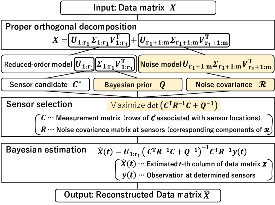
The approach and the contribution of the present study are illustrated in Fig. 1.
Firstly, basics of the POD-based reduced-order modeling and sparse sensing are briefly revisited. Algorithms of the previous and the present study are given in sections 2.1 and 2.2, and then the superiority of the proposed method for noisy datasets is shown by reproducing randomly generated data matrices and other datasets of actual measurements in section 3. Finally, section 4 concludes the paper.
2 Formulations and Algorithms
2.1 Reduced-order modeling, sparse sensing and the previous greedy optimization of sensor placement
First, observations are linearly constructed from parameters as:
| (1) |
Here, , and are an observation vector, a parameter vector and a given measurement matrix, respectively. It should also be noted that the absence of noise is assumed in Eq. 1. The estimated parameters (a quantity with hat refers to the estimated value of the quantity) can be obtained by a pseudo inverse operation.
| (4) |
Then, uncorrelated Gaussian noise of the same variance and zero mean for every observation point is considered. Joshi and Boyd [13] clearly showed an objective function to design the best estimation system for the case . They aimed to maximize a logarithm of the determinant of the Fisher information matrix, which realised the least ellipsoid volume of the expected estimation error , as in Eq. 5
| maximize | (5) |
Additionally, there have been many studies adopting those optimization problems to low-order but high-dimensional data. The measurement matrix in Eq. 1 becomes , where is a total measurement matrix (or, in other words, a sensor candidate matrix) for whole observation candidates and as a sensor-location matrix that gives observe locations among candidates. Equation 5 is now interpreted as a searching problem of the most effective locations of sensors by determining if is given. Basically, all the combinations of sensors out of sensor candidates should be searched by the brute-force algorithm for the real-optimized solution of Eq. 5, which takes enormous computational time ().
Instead, greedy algorithms for suboptimized solutions by adding a sensor step by step has been devised for reduced-order modeling [15]. As many studies did, Saito et al. [16] set to be the reduced-order spatial-mode matrix in Eq. 10 that proper orthogonal decomposition (POD) generated from given training data, which consists of snapshots for variables . With matrix, a greedy selection was demonstrated as shown in Algorithm 1 to pursue Eq. 5. A data matrix and its reduced-order representation are given by singular value decomposition (SVD):
| (9) | ||||
| (10) | ||||
and are a diagonal matrix of the singular values and a matrix of the temporal modes, respectively, and the subscript notation for a given matrix denotes a low-rank representation of , using the th-to-th singular values or vectors. It should be noted that POD can be processed by SVD if spatial and temporal desensitization of the data are uniform.
Here, and refer a set of indices for locations of the sensor candidates and its subset of the determined sensors, respectively. Additionally, the notation for an arbitrary quantity indicates a quantity that its th component is to be investigated in this step-wise selection, with the components given by the selected sensors. After the th selection step, is constructed by the sensors selected. As an example, and are written as follows:
| (12) | |||||
| (13) |
where and indicate an index of the th selected sensor location and the corresponding row vector of the sensor-candidate matrix , respectively. In Ref. [16], maximization of the determinant of the Fisher information matrix of both cases in Eq. 4 are realized with the matrix determinant lemma which quickens the computation as shown in Algorithm 1.
This approach effectively works, but sometimes does not as experienced in Ref. [16], and as demonstrated later in a tested problem of section 3. That defect arises because the linear least squares estimation that a large number of studies employed, misses information in data such as an expected distribution of parameters . Here, in our problem will be amplitudes of principal POD modes at arbitrary time. Consequently, the same levels of the amplitudes of low- to high-order modes as each other are assumed although the matrix in Eq. 10 shows that they differ. Moreover, the aspects are not considered in the previous straightforward implementation that the observation is always contaminated with the truncated POD modes (see matrices in the second term of Eq. 10), and that they cause spatially correlated noise for the reduced-order estimation Eq. 4.
2.2 Bayesian Estimation using Sparse Sensor
In Ref. [21], a proper objective function for the selection is derived under an assumption of the correlated noise. Although they formulated optimization considering such noise, noise itself is only given as a function of distance between sensors. A data-driven method for the modeling of the correlated noise are presented in this paper and two more conditions are exploited for a more robust estimation; one is expected variance of the POD mode amplitudes, and the other is spatial covariance of the components that are truncated in the order reduction of data matrix Eq. 10. The former can be estimated from as:
| (14) |
where is the expectation value of a variable . Then, full-state observation and covariance matrix of the noise become
| (15) |
where is a observation noise vector and is one snapshot (one column vector) of . The sparse observation and its noise covariance are:
| (16) |
where represents a covariance matrix of the noise that sensors capture. Here, the full-state noise covariance is assumed to be estimated from the high-order modes:
| (17) |
and
| (18) |
Then, the Bayesian estimation is derived with those prior information. Here,an a priori probability density function (PDF) of the POD mode amplitudes becomes:
| (19) |
and the conditional PDF of under given is as follows:
| (20) |
These relations lead to the a posteriori PDF:
| (21) |
Here, the maximum a posteriori estimation on is:
| (22) |
Thanks to the normalization term , the inverse operation in Eq. 22 is regular for any conditions of unlike the least squares estimation in Eq. 4. In this estimation, the objective function in the Eq. 5 is modified:
| (23) |
Note that sensors should be removed from candidates if they have extremely low signal fluctuations. This is because those sensors increase the objective value Eq. 23 by making the matrix singular. In the present study, the locations are beforehand excluded from for simplicity if their RMSs are times smaller than the maximum of the dataset, and denotes a subset of after this exclusion.
Note that for the case is a diagonal matrix, Joshi and Boyd [13] have already derived a convex optimization of the sensor selection for the Bayesian estimation. In the present study, includes nondiagonal components which represent the correlation in measurement noise.
The proposed method suppresses correlated measurement noise by considering . This Bayesian determinant-based greedy (BDG) algorithm is presented in Algorithm 2. Here, row vector refers to the th sensor location that has unity in the th component with zero in the others, which extracts the th row vector from the sensor-candidate matrix .
2.3 Fast algorithm
A fast implementation is considered based on Algorithm 2 as Saito et al. demonstrated in their determinant calculation using rank-one lemma [16]. First, the covariance matrix generated by the th sensor candidate in the th sensor selection, is:
| (26) |
where the covariance of noise between the sensor candidate and the selected sensors is
| (27) |
and similarly, the variance of noise at the location is
| (28) |
Here, is the optimized first-to-()th-sensor selection matrix. In addition, is determined in the previous th step. Accordingly, is obtained as follows:
| (31) |
where
The objective function is now considered based on the expressions above.
| (37) | ||||
| (38) | ||||
Because and its determinant have already been obtained in the previous step, the th sensor can be selected by the following scalar evaluation:
| (39) |
Once the sensor is selected, and are updated. This algorithm is described in Algorithm 3 including another improvement for computational efficiency which is introduced in the next subsection.
2.4 Memory Efficient Implementation
As was already introduced in Eq. 17, the covariance of noise for every pair of observation points can be estimated by multiplying and , and then stored to be . In Algorithm 2, and are constructed by taking the corresponding parts of . Although this could be a straightforward way to calculate and , it often runs out memory storage to store since , the size of , can often reach billions or more in an actual application.
Therefore, the following implementation is proposed by reducing the order of the noise covariance from to : only diagonal components of is constructed and stored as a -components vector , and is approximated for every loop by using the dominant first columns of in Eq. 17. This modification is reasonable because nondiagonal components are inherently small compared to diagonal ones of , thereby modes have less effect on the as the mode number increases. Here, an appropriate should be determined with consideration on characteristics of the data matrix. The effects of truncating of are shown in section 3.3.
Then, is approximated:
| (40) |
where, and are the leading columns of the remainder spatial modes matrix and first components of the remainder singular value matrix . These processes are called the truncation. This approximation simply reduces amount of stored memory and computational complexity. These modifications in section 2.3 and section 2.4 are integrated into the Algorithm 3. A comparison on computing complexity of the methods introduced thus far are listed in Table 1.
| Name | Complexity | |
|---|---|---|
| Brute-force | ||
| DG | [Algorithm 1] | |
| BDG | [Algorithm 2] | |
| Fast-BDG | [Algorithm 3] |
3 Applications
3.1 Sensors for randomized matrix
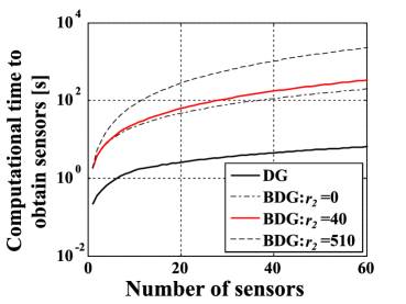
The numerical experiments were conducted and the proposed method were verified. The random data matrices, , were set, where and consist of 500 orthogonal vectors that were generated by QR decomposition of normally distributed random matrices, and components of diagonal matrix are , respectively. These slowly decaying diagonal components of are simulating the data of an actual flow field. The following results of measuring computational time to obtain sensors demonstrated in sections 3.1 and 3.3 are conducted under the environments as listed in section 3.1.
[htbp] Computing environments to measure computational time Specification Randomized matrix NOAA-SST Processor information Intel(R) Core(TM) Intel(R) Core(TM) S@GHz K@GHz Random access memory GB GB System type bit operating system bit operating system x64 base processor x64 base processor Program code Matlab R2013a Operating system Linux Mint Tessa Windows 10 Pro Version: 19.1 Version:1890
First, the reconstruction error which is used throughout the paper is defined as follows:
| (41) |
where the numerator and denominator are norm of residual and that of the original state, respectively.
Figure 2a illustrates the computational time for the sensor selection. This figure shows the increases in computational cost as indicated in Table 1.
| DG | [Algorithm 1] | |
|---|---|---|
| BDG | [Algorithm 2] |


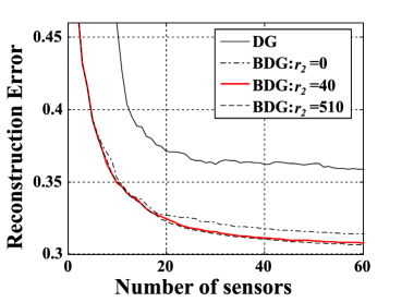
In addition, the comparison on estimation error defined in Eq. 41 was conducted. The effectiveness of Bayesian estimation in Eq. 22 and the BDG sensor selection in Eq. 39 were independently investigated in Fig. 2b. The estimation methods and the sensor selection methods are presented in Tables 2a and 2b, and note that DG-LSE (DG and the least squares estimation) and BDG-BE (BDG and the Bayesian estimation) are optimum combinations under the framework of LSE and BE, respectively. Two more combinations of the methods were tested for verification, namely DG-BE and BDG-LSE.
Figure 2b illustrates that the Bayesian estimation plays an important role, since the DG-BE result is better than that of DG-LSE although correlated noise is not considered in the selection. In contrast, the error of LSE increases around regardless of the choice of DG or BDG. Errors around increase because the observed signal by the sensors is strictly converted into the latent amplitudes of POD modes despite they contain intense correlated noise of higher modes. The components in the smallest-sensitivity direction should also be estimated which includes the larger error due to the noise, whereas the components in that direction are assumed to be zero in the pseudo-inverse operation and such an error is suppressed when . The error of BDG-LSE is the largest in the range of because the sensors of BDG are chosen with assuming the regularization of the Bayesian estimation, and therefore the smallest-sensitivity direction components of least squares estimation are not accurately predicted in BDG-LSE than in DG-LSE. However, BDG-LSE works sligtly better than, or at least equal to, DG-LSE in the condition of . This is because BDG choose the sensor which is less contaminated by correlated noise and such sensors work better even in the LSE. Finally, the error of BDG-BE is always the smallest in these four methods. This illustrates that BDG choose the sensor positions suitable to the Bayesian estimation Eq. 22.
3.2 Sensors for flow around airfoil
The particle image velocimetry (PIV) was previously conducted and time-resolved data of velocity fields around an airfoil were obtained[23]. The effectiveness of the present method for the PIV data is demonstrated hereafter. The test conditions are listed in Table 3 and the fluctuating components of the freestream direction velocity is only employed, unlike the previous study in which the two-dimensional velocity is simultaneously treated [24].
| Laser | Double pulse lasers |
|---|---|
| Time between pulse | s |
| Sampling rate | Hz |
| Particle image resolution | pixels |
| Total number of image pairs |
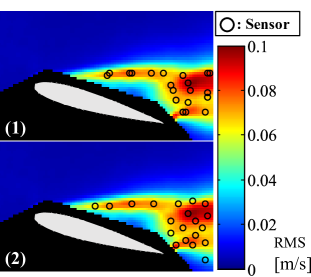
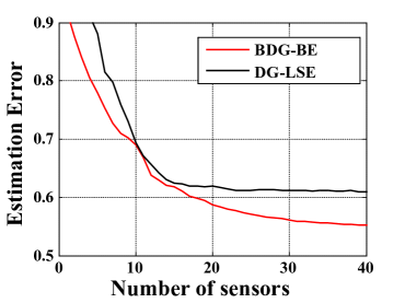
Figure 3a clearly shows that the present method selects different sensor positions from those selected by the previous algorithm. The region of high RMS in the temporal series data is red-colored in the figure. The selected sensor positions of the previous method tend to be concentrated in small parts of highly fluctuated recirculation regions, whereas those of the presented method are located evenly in those regions. A comparison of the reconstruction error using the first 10 modes illustrates that the proposed method is effective and its error approaches the lower limit of error estimated by full observation.
3.3 Sensors for sea surface temperature distribution
The sea surface temperature (SST) data are distributed at the NOAA website [25]. The data formatted by Manohar et al. [15] are adopted in the present study. The details of the data are listed in Table 4.
| Brief Description | NOAA Optimum Interpolation (OI) SST V2 [25] |
|---|---|
| Temporal Coverage | Weekly means from 1989/12/31 to 1999/12/12 |
| ( snapshots) | |
| Spatial Coverage | 1.0 degree latitude x 1.0 degree longitude |
| global grid ( observed points) |
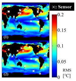
As was conducted in section 3.2, ten modes are employed for the reduced-order modeling after trimming the low RMS points off from the sensor candidates as described in section 2.2. Fig. 4a shows the difference in sensor positions as indicated by cross marks, and backgrounds are time-series RMS of SST data. Those figures show that the sensors are so scattered by the proposed method that the effects of the correlated noise due to truncated POD modes could be minimized.
The effect of truncation for an efficient memory implementation is also demonstrated in this section as introduced in section 2.4. Because the SST dataset consists of a enormous number of observation locations , and it requires considerable time to calculate Eq. 15. The variation of the reconstruction error and the computational time are shown in Figures 4b and 4c. Those results of the BDG sensors are calculated for three cases, , , . Especially, and correspond to the case ignoring all the nondiagonal terms of , and the case Eq. 15, respectively. As expected, these plots show that more accurate estimation is realized when higher modes are used for noise covariance, but it indeed needs longer calculation time. A reasonable which leads to both less calculation time and less reconstruction error appears to be around , only of the original modes. The general criteria of reasonable parameter should be addressed in future research.
4 Conclusions
In the context of Bayesian maximum a posteriori (MAP) state estimation, a greedy selection method for noise-robust sensors is proposed for the reconstruction of the high-dimensional data. The algorithm leverages high-order modes of the singular value decomposition of data, which were ignored in the previous reduced-order sensing framework, for the construction of the noise covariance matrix used as weights in the MAP state estimation. Prior distribution of coefficients are also generated from information of the modes. The proposed method determines sensors by maximizing the determinant of a matrix in the MAP estimation operator, which simultaneously minimizes a metric of expected estimation error. Additionally, the rank-one lemma and a low-rank approximation of the covariance matrix are considered for more efficient implementation.
Our approach was applied to some examples and the reconstruction ability of determined sensors were verified. Firstly, we separately confirmed noise-robustness of sensors of the proposed method and benefits of the Bayesian estimation. Reproduction results on data matrices showed significant improvement in reconstruction accuracy with reasonable increase in the computational time, compared with that of the previously presented method.
Future works of interest are including;
-
1.
To extend the method to nonlinear measurement. This method is based on a linear modeling of POD modes, hence it should be extended to more generalized measurement configuration like [7].
-
2.
To adopt various noise models such as an exponential model from the same reason above.
-
3.
To involve dynamics of phenomena into modeling, estimation and sensor selection. This should be considered for feedback control. Some metrics associated with observability and controllablity were proposed in Ref. [26], and the extension of the present work to these metrics is in our future focus.
Acknowledgements
This work was partially supported by JST CREST Grant Number JPMJCR1763, Japan. The fourth author T.N. is grateful for support of the grant JPMJPR1678 of JST Presto, Japan.
References
- [1] R. K. Kincaid, S. L. Padula, D-optimal designs for sensor and actuator locations, Computers & Operations Research 29 (6) (2002) 701–713. doi:10.1016/S0305-0548(01)00048-X.
- [2] T. C. Corke, M. L. Post, D. M. Orlov, Sdbd plasma enhanced aerodynamics: concepts, optimization and applications, Progress in Aerospace Sciences 43 (7-8) (2007) 193–217. doi:10.1016/j.paerosci.2007.06.001.
- [3] R. Bates, R. Buck, E. Riccomagno, H. Wynn, Experimental design and observation for large systems, Journal of the Royal Statistical Society: Series B (Methodological) 58 (1) (1996) 77–94. doi:10.1111/j.2517-6161.1996.tb02068.x.
- [4] S. L. Brunton, J. H. Tu, I. Bright, J. N. Kutz, Compressive sensing and low-rank libraries for classification of bifurcation regimes in nonlinear dynamical systems, SIAM Journal on Applied Dynamical Systems 13 (4) (2014) 1716–1732.
- [5] F. E. Udwadia, Methodology for optimum sensor locations for parameter identification in dynamic systems, Journal of engineering mechanics 120 (2) (1994) 368–390. doi:10.1061/(ASCE)0733-9399(1994)120:2(368).
- [6] S. L. Brunton, J. L. Proctor, J. N. Kutz, Discovering governing equations from data by sparse identification of nonlinear dynamical systems, Proceedings of the national academy of sciences 113 (15) (2016) 3932–3937. doi:10.1073/pnas.1517384113.
- [7] S. Chaturantabut, D. C. Sorensen, Nonlinear model reduction via discrete empirical interpolation, SIAM Journal on Scientific Computing 32 (5) (2010) 2737–2764. doi:10.1137/090766498.
- [8] R. Semaan, Optimal sensor placement using machine learning, Computers & Fluids 159 (2017) 167–176. doi:10.1016/j.compfluid.2017.10.002.
- [9] G. Berkooz, P. Holmes, J. L. Lumley, The proper orthogonal decomposition in the analysis of turbulent flows, Annual review of fluid mechanics 25 (1) (1993) 539–575. doi:10.1146/annurev.fl.25.010193.002543.
- [10] B. Peherstorfer, Z. Drmac, S. Gugercin, Stability of discrete empirical interpolation and gappy proper orthogonal decomposition with randomized and deterministic sampling points (2018). arXiv:1808.10473.
- [11] K. Nakai, K. Yamada, T. Nagata, Y. Saito, T. Nonomura, Effect of objective function on data-driven sparsesensor optimization (2020). arXiv:2007.05377.
- [12] L. Ye, S. Roy, S. Sundaram, On the complexity and approximability of optimal sensor selection for kalman filtering, in: 2018 Annual American Control Conference (ACC), IEEE, 2018, pp. 5049–5054. doi:10.23919/ACC.2018.8431016.
- [13] S. Joshi, S. Boyd, Sensor selection via convex optimization, IEEE Transactions on Signal Processing 57 (2) (2009) 451–462. doi:10.1109/TSP.2008.2007095.
- [14] T. Nonomura, S. Ono, K. Nakai, Y. Saito, Randomized subspace newton convex method applied to data-driven sensor selection problem (2020). arXiv:2009.09315.
- [15] K. Manohar, B. W. Brunton, J. N. Kutz, S. L. Brunton, Data-driven sparse sensor placement for reconstruction: Demonstrating the benefits of exploiting known patterns, IEEE Control Systems Magazine 38 (3) (2018) 63–86. doi:10.1109/MCS.2018.2810460.
- [16] Y. Saito, T. Nonomura, K. Yamada, K. Asai, Y. Sasaki, D. Tsubakino, Determinant-based fast greedy sensor selection algorithm (2019). arXiv:1911.08757.
- [17] N. K. Dhingra, M. R. Jovanović, Z.-Q. Luo, An admm algorithm for optimal sensor and actuator selection, in: 53rd IEEE Conference on Decision and Control, IEEE, 2014, pp. 4039–4044. doi:10.1109/CDC.2014.7040017.
- [18] T. Nagata, T. Nonomura, K. Nakai, K. Yamada, Y. Saito, S. Ono, Data-driven sparse sensor placement based on a-optimal design of experiment with admm (2020). arXiv:2010.09329.
- [19] M. O’Connor, W. B. Kleijn, T. Abhayapala, Distributed sparse mvdr beamforming using the bi-alternating direction method of multipliers, in: 2016 IEEE International Conference on Acoustics, Speech and Signal Processing (ICASSP), IEEE, 2016, pp. 106–110. doi:10.1109/ICASSP.2016.7471646.
- [20] R. Castro-Triguero, S. Murugan, R. Gallego, M. I. Friswell, Robustness of optimal sensor placement under parametric uncertainty, Mechanical Systems and Signal Processing 41 (1-2) (2013) 268–287. doi:10.1016/j.ymssp.2013.06.022.
- [21] S. Liu, S. P. Chepuri, M. Fardad, E. Maşazade, G. Leus, P. K. Varshney, Sensor selection for estimation with correlated measurement noise, IEEE Transactions on Signal Processing 64 (13) (2016) 3509–3522. doi:10.1109/TSP.2016.2550005.
- [22] D. Uciński, D-optimal sensor selection in the presence of correlated measurement noise, Measurement 164 (2020) 107873. doi:10.1016/j.measurement.2020.107873.
- [23] K. Nankai, Y. Ozawa, T. Nonomura, K. Asai, Linear reduced-order model based on piv data of flow field around airfoil, TRANSACTIONS OF THE JAPAN SOCIETY FOR AERONAUTICAL AND SPACE SCIENCES 62 (4) (2019) 227–235. doi:10.2322/tjsass.62.227.
- [24] Y. Saito, T. Nonomura, K. Nankai, K. Yamada, K. Asai, Y. Sasaki, D. Tsubakino, Data-driven vector-measurement-sensor selection based on greedy algorithm, IEEE Sensors Letters 4 (2020). doi:10.1109/LSENS.2020.2999186.
-
[25]
NOAA/OAR/ESRL,
Noaa
optimal interpolation (oi) sea surface temperature (sst) v2 (July 2019).
URL https://www.esrl.noaa.gov/psd/data/gridded/data.noaa.oisst.v2.html - [26] T. H. Summers, F. L. Cortesi, J. Lygeros, On submodularity and controllability in complex dynamical networks, IEEE Transactions on Control of Network Systems 3 (1) (2015) 91–101. doi:10.1109/TCNS.2015.2453711.