Percolation of three fluids on a honeycomb lattice

Abstract

In this paper, we consider a generalization of percolation: percolation of three related fluids on a honeycomb lattice. K. Izyurov and A. Magazinov proved that percolations of distinct fluids between opposite sides on a fixed hexagon become mutually independent as the lattice step tends to $0$. This paper exposes this proof in details (with minor simplifications) for nonspecialists. In addition, we state a few related conjectures based on numerical experiments.

Keywords— Fourier-Walsh transform, Potts model, percolation, honeycomb lattice, Boolean functions.

1 Introduction

In this paper, we consider a generalization of percolation: percolation of three related fluids on a honeycomb lattice. We prove (see Theorem 1) that percolations of distinct fluids between opposite sides of a fixed hexagon become mutually independent as the lattice step tends to $0$. This was a conjecture by M. Skopenkov proved independently by K. Izyurov and A. Magazinov approximately at the same time (private communication). The proof is based on the Fourier-Walsh expansion and Kesten’s theorem. This paper exposes this proof in details (with minor simplifications) for nonspecialists. We also state a few new related conjectures based on numerical experiments.

The paper is organized as follows. In §2, we introduce key definitions, and also state Main Theorem 1 and several conjectures. In §3, we introduce the Fourier-Walsh expansion. In §4, we expose the proof of Theorem 1 based on the Fourier-Walsh expansion. In §5, we describe results of numerical experiments related to conjectures from §2.

2 Main theorem

For any $n>1$ consider a honeycomb lattice of step $\frac{1}{n}$. Let $P$ be a regular hexagon with the side $1$ centered at the center of some cell $O$. Denote by $M_{n}$ the set of all the cells contained in $P$. Consider the probability space $\Omega$ consisting of all the colorings of the cells of the set $M_{n}$ into $4$ colors, denoted by $0$, $1$, $2$, $3$, with the measure $P(B)=|B|/4^{|M_{n}|}$ for any $B\subset\Omega$. The probability space $\Omega$ is called the four-state Potts model at infinite temperature.

Definition 1.

Fix a number $k=1$, $2$ or $3$, and also a coloring of the cells of the set $M_{n}$ into $4$ colors. We say that fluid $k$ percolates between two sets $A,B\subset~{}M_{n}$, if some cell of the set $A$ is joined with some cell of the set $B$ by a chain of adjacent cells such that each cell in the chain has color $0$ or $k$, including the initial cell of the set $A$ and the final cell of the set $B$.

2.1 Percolation between sides

We say that a cell $x\in M_{n}$ belongs to a side $A$ of the hexagon $P$, if the cell $x$ is a boundary cell and $A$ is the nearest side to $x$. A cell can belong to more than one side (if the cell has several nearest sides). In what follows, by side $A$ we mean the set of all the cells belonging to the side $A$ of the hexagon $P$.

Label the sides of the hexagon $P$ by numbers from $1$ to $6$ counterclock-wise. For $k=1,2$ or $3$ denote by $B_{k,n}\subset\Omega$ the set of all the colorings such that fluid $k$ percolates between sides $k$ and $k+3$ of the hexagon $P$. It is easy to show that events $B_{1,n},B_{2,n},B_{3,n}$ are pairwise independent: $P(B_{1,n}\cap B_{2,n})-P(B_{1,n})P(B_{2,n})=0$.

Theorem 1 (K. Izyurov, A. Magazinov, 2018).

$${\lim_{n\to+\infty}}\left[P(B_{1,n}\cap B_{2,n}\cap B_{3,n})-P(B_{1,n})P(B_{2,n})P(B_{3,n})\right]=0.$$

Remark 1.

Theorem 1 holds in a much more general situation. For example, a regular hexagon $P$ can be replaced by an arbitrary polygon, and opposite sides can be replaced by arbitrary pairs of sides. Nevertheless, for simplicity of the proof, we consider percolation between opposite sides of a regular hexagon.

Informally, Theorem 1 states that percolations of distinct fluids between opposite sides become mutually independent as $n$ tends to $\infty$. We take a difference of probabilities rather than a ratio to avoid proving that $P(B_{1,n})P(B_{2,n})P(B_{3,n})$ is bounded from zero.

In addition, we state the following conjecture.

Conjecture 1.

$P(B_{1,n}\cap B_{2,n}\cap B_{3,n})\geqslant P(B_{1,n})P(B_{2,n})P(B_{3,n})$ for each $n$.

Since events $B_{1,n},B_{2,n},B_{3,n}$ are independent, the conjecture states that percolations of distinct fluids are positively correlated, i.e.,

$$P(B_{1,n}|B_{2,n}\cap B_{3,n})\geqslant B_{1,n}.$$

2.2 Percolation from the center

Definition 2.

Fix a number $k=1$, $2$ or $3$, and also a coloring of the cells of the set $M_{n}$ into $4$ colors. We say that fluid $k$ percolates from a cell $x\in M_{n}$ to a set $A\in M_{n}$, if $x$ is joined with some cell of the set $A$ by a chain of adjacent cells such that each cell in the chain has color $0$ or $k$, including the final cell of the set $A$ and not including the initial cell $x$.

Note that in Definition 2, unlike Definition 1, the color of the initial cell $x$ does not matter. That is convenient to avoid a factor of $2$ in the inequalities of Conjectures 2 and 3 below.

For $k=1,2$, and $3$ denote by $A_{k,n}\subset\Omega$ the set of colorings such that fluid $k$ percolates from the cell $O$ to the set of all the boundary cells of the set $M_{n}$.

Let us state 2 conjectures.

Conjecture 2.

$P(A_{1,n}\cap A_{2,n}\cap A_{3,n})\geqslant P(A_{1,n})P(A_{2,n})P(A_{3,n})$ for each $n$.

Conjecture 3.

$\displaystyle{\lim_{n\to+\infty}}\frac{P(A_{1,n}\cap A_{2,n}\cap A_{3,n})}{P(A_{1,n})P(A_{2,n})P(A_{3,n})}>1$.

In addition, we state one more conjecture that generalizes Conjectures 1 and 2.

Conjecture 4.

Let $A_{1},A_{2},A_{3},B_{1},B_{2},B_{3}\subset M_{n}$. Denote by $U_{k}=$ {fluid $k$ percolates between $A_{k}$ and $B_{k}$}. Then

$$P(U_{1}\cap U_{2}\cap U_{3})\geqslant P(U_{1})P(U_{2})P(U_{3}).$$

If Conjecture 4 is true, then $P(U_{1}|U_{2}\cap U_{3})\geqslant P(U_{1})$, i.e., percolations between any three pairs of subsets are positively correlated.

2.3 Example

Figure 1:

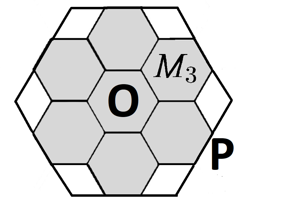
We illustrate the above notions by an example.

Example 1.

Let $n=3$. In Figure 1 we see a regular hexagon $P$ on a honeycomb lattice of step $\frac{1}{3}$. The set $M_{3}$ consists of 7 gray cells. It is easy to show that

$$P(A_{1,3})=P(A_{2,3})=P(A_{3,3})=1-\left(\frac{1}{2}\right)^{6}=0,984375;$$

$$P(A_{1,3}\cap A_{2,3}\cap A_{3,3})=1-3\left(\frac{1}{2}\right)^{6}+3\left(\frac{1}{2}\right)^{12}=0,953857421875;$$

$$P(B_{1,3})=P(B_{2,3})=P(B_{3,3})=\frac{1}{4}\left(\frac{1}{2}+\frac{1}{2}\cdot\frac{7}{16}\right)=\frac{23}{128}=0,1796875;$$

$$P(B_{1,3}\cap B_{2,3}\cap B_{3,3})=\frac{1}{4}\cdot\left(\frac{1}{2}\right)^{6}+\frac{3}{4}\cdot\left(9\left(\frac{1}{4}\right)^{6}+2\left(\frac{1}{2}\right)^{2}\left(\frac{1}{4}\right)^{4}\right)=0,00701904296875.$$

Then

$$\frac{P(A_{1,3}\cap A_{2,3}\cap A_{3,3})}{P(A_{1,3})P(A_{2,3})P(A_{3,3})}=\frac{250048}{250047}>1\text{ and }$$

$$P(B_{1,3}\cap B_{2,3}\cap B_{3,3})-P(B_{1,3})P(B_{2,3})P(B_{3,3})\approx 0,01.$$

This agrees with Conjectures 1 and 2, and also show that both events $A_{1,3},A_{2,3},A_{3,3}$ and events $B_{1,3},B_{2,3},B_{3,3}$ are mutually dependent.

2.4 Kesten’s Theorem

The model introduced above naturally generalizes the classical percolation model (when cells are paint into 2 colors). In that model, the following famous result, used in the proof of Theorem 1, holds.

Definition 3 (cf. Definition 2).

Paint cells of some finite set $M$ into $2$ colors $\pm 1$. We say that there exists percolation from a cell $x\in M$ to a set $A\subset M$ for that coloring, if $x$ is joined with some cell of the set $A$ by a chain of adjacent cells such that each cell in the chain has color $+1$, including the final cell of the set $A$ and not including the initial cell $x$. We introduce the measure $P(B)~{}=~{}|B|/2^{m}$ on the set of all the colorings of the set $M$ into 2 colors.

Theorem 2.

(H. Kesten, 1982, cf. [5, Theorem 9.6]). The probability that there exists percolation from the cell $O$ to the boundary of the set $M$ tends to $0$ as $n\to\infty$.

3 The Fourier-Walsh expansion

In this section, we introduce the notion of the Fourier-Walsh expansion and consider some properties of the coefficients of that expansion. The content of §§3.1-3.3 is borrowed from [1, §§1.2-1.4]. Lemma 7 from §3.4 is similar to a result from [1, §2.2]. Lemma 8 from §3.4 is contained in [1, §3.6] as an exercise.

Agreement.

In what follows, on the set $\{-1,+1\}^{m}$, where $m~{}\in~{}\mathbb{N}$, fix the measure $P(B)=|B|/2^{m}$ for any $B\subset\{-1,+1\}^{m}$. Functions $f\colon\{-1,+1\}^{m}\to\mathbb{R}$ are considered as random variables on $\{-1,+1\}^{m}$.

3.1 Definition

Definition 4.

Let $m\in\mathbb{N}$. The Fourier-Walsh expansion of a function

$$f\colon\{-1,+1\}^{m}\to\mathbb{R}$$

is its representation as the sum

$$f(x_{1},\ldots,x_{m})=\sum_{S\subset\{1,2,\ldots,m\}}\widehat{f_{S}}\prod_{i\in S}x_{i},$$

where $\widehat{f_{S}}$ are some real numbers that are called the Fourier-Walsh coefficients. If $S=\varnothing$, then we put by definition $\prod_{i\in S}x_{i}=1$.

Remark 2.

In what follows, we write $\widehat{f_{S}}$ for the coefficient of a term $\prod_{i\in S}x_{i}$ in the Fourier-Walsh expansion of a function $f\colon\{-1,+1\}^{m}\to\mathbb{R}$.

Theorem 3.

For any $f\colon\{-1,+1\}^{m}\to\mathbb{R}$, there exists a unique Fourier-Walsh expansion.

Proof.

Existence. For each point $a=(a_{1},a_{2},\ldots,a_{m})\in\mathbb{R}^{m}$, where $a_{i}=\pm 1$, consider the function

$$1_{a}(x_{1},x_{2},\ldots,x_{m})=\left(\frac{1+a_{1}x_{1}}{2}\right)\left(\frac{1+a_{2}x_{2}}{2}\right)\cdots\left(\frac{1+a_{m}x_{m}}{2}\right),$$

where $x_{i}=\pm 1$. Note that

$$1_{a}(x)=\begin{cases}$1$,&\text{if }x=a;\\ $0$,&\text{otherwise.}\end{cases}$$

Therefore, any function $f:\{-1,+1\}^{m}\rightarrow\mathbb{R}$ can be written as

$$f(x)={\sum_{a\in\{-1,+1\}^{m}}}f(a)1_{a}(x).$$

Expanding this expression we obtain the required expansion.

Uniqueness. All the functions $f:\{-1,+1\}^{m}~{}\rightarrow~{}\mathbb{R}$ form a $2^{m}$-dimensional vector space. And there are exactly $2^{m}$ monomials of a form $\prod_{i\in S}x_{i}$, where $S~{}\subset~{}\{1,2,\ldots,m\}$. Since any function is a linear span of such monomials, it follows that these monomials form a basis. Hence the Fourier-Walsh coefficients are unique. ∎

3.2 A formula for the Fourier-Walsh coefficients

In this section, we introduce a formula for the Fourier-Walsh coefficients in terms of the expectation of a random variable (Lemma 4 below).

Notation 1.

Let $S\subset\{1,2,\ldots,m\}$. Denote by $\sigma_{S}$ the function $\sigma_{S}~{}\colon~{}\{-1,+1\}^{m}~{}\to~{}\{-1,+1\}$ given by the formula $\sigma_{S}(x_{1},\ldots,x_{m})=\prod_{i\in S}x_{i}$.

Lemma 1.

Let $S,T\subset\{1,2,\ldots,m\}$. Then $\sigma_{S}\sigma_{T}=\sigma_{S\triangle T}$.

Proof.

We have $\sigma_{S}\sigma_{T}=\displaystyle{\prod_{i\in S}x_{i}\prod_{j\in T}x_{i}=\prod_{i\in S\cap T}x_{i}^{2}\prod_{j\in S\triangle T}x_{i}}=\prod_{j\in S\triangle T}x_{i}=\sigma_{S\triangle T}.$ ∎

Lemma 2.

The random variables $\sigma_{\{1\}},\sigma_{\{2\}},\ldots,\sigma_{\{m\}}$ have expectation $0$ and are mutually independent.

The proof of this lemma is obvious.

Lemma 3.

Let $S\subset\{1,2,\ldots,m\}$. Then

$$\mathbb{E}\sigma_{S}=\begin{cases}$1$,&\text{if }S=\varnothing;\\ $0$,&\text{otherwise.}\end{cases}$$

Proof.

If $S=\varnothing$, then $\mathbb{E}\sigma_{\varnothing}=\mathbb{E}1=1$.

If $S\neq\varnothing$, then by Lemma 2 we have

$$\mathbb{E}(\sigma_{S})=\mathbb{E}\prod_{i\in S}x_{i}=\prod_{i\in S}\mathbb{E}x_{i}=0.$$

∎

Lemma 4 (The formula for the Fourier-Walsh coefficients).

Let $T\subset\{1,2,\ldots,m\}$. Then for any function $f\colon\{-1,+1\}^{m}\to\mathbb{R}$ we have $\widehat{f_{T}}=\mathbb{E}(f\sigma_{T})$.

Proof.

By Definition 4, Lemmas 1 and 3 we get

$$\mathbb{E}(f\sigma_{T})=\mathbb{E}\left[\sigma_{T}\cdot\displaystyle{\sum_{S\subset\{1,2,\ldots,m\}}}\widehat{f_{S}}\cdot\sigma_{S}\right]=\mathbb{E}\left[\displaystyle{\sum_{S\subset\{1,2,\ldots,m\}}}\widehat{f_{S}}\cdot\sigma_{S\triangle T}\right]=\widehat{f_{T}}.$$

∎

3.3 Variance

In this section, we prove an important formula, which shows a relation between the variance of a Boolean function and the Fourier-Walsh coefficients of this function (Corollary 1 below). First we prove a simple fact.

Lemma 5.

For any function $f\colon\{-1,+1\}^{m}\to\{0,1\}$ we have $0\leqslant Var(f)\leqslant 1.$

Proof.

Obviously, $\mathbb{E}f\in[0,1]$. Hence $Var(f)=\mathbb{E}(f^{2})-(\mathbb{E}f)^{2}=\mathbb{E}f-(\mathbb{E}f)^{2}\in[0,1].$ ∎

Lemma 6.

For any function $f\colon\{-1,+1\}^{m}\to\mathbb{R}$ we have $\mathbb{E}(f^{2})=\sum_{S\subset\{1,\ldots,m\}}\widehat{f_{S}}^{2}$.

Proof.

By Lemmas 1 and 3 we get

$$\mathbb{E}(f^{2})=\mathbb{E}\left[\sum_{S\subset\{1,2,\ldots,m\}}\widehat{f_{S}}\sigma_{S}\right]^{2}=\mathbb{E}\left(\sum_{S\subset\{1,2,\ldots,m\}}\widehat{f_{S}}^{2}\sigma_{S}^{2}+2\underset{S\neq T}{\sum_{S,T\subset\{1,2,\ldots,m\}}}\widehat{f_{S}}\widehat{f_{T}}\sigma_{S\triangle T}\right)=\sum_{S\subset\{1,\ldots,m\}}\widehat{f_{S}}^{2}.$$

∎

Corollary 1.

For any function $f\colon\{-1,+1\}^{m}\to\mathbb{R}$ we have

$$Var(f)=\underset{S\neq\varnothing}{\sum_{S\subset\{1,\ldots,m\}}}\widehat{f_{S}}^{2}.$$

Proof.

Since $\sigma_{\varnothing}=1$, by Lemmas 4 and 6 it follows that

$$Var(f)=\mathbb{E}(f^{2})-(\mathbb{E}f)^{2}=\underset{S\neq\varnothing}{\sum_{S\subset\{1,\ldots,m\}}}\widehat{f_{S}}^{2}.$$

∎

3.4 Increasing Boolean functions

In this section, we consider only functions with the values in $\{0,1\}$.

Definition 5.

Let $a=(a_{1},a_{2},\ldots,a_{m}),b=(b_{1},b_{2},\ldots,b_{m})\in\{-1,1\}^{m}$. We write $a\leqslant b$, if for each $i=1,\ldots,m$ we have $a_{i}\leqslant b_{i}$. A function $f\colon\{-1,+1\}^{m}\to\{0,1\}$ is called increasing, if the inequality $a\leqslant b$ implies the inequality $f(a)~{}\leqslant~{}f(b).$

Definition 6.

We say that a coordinate $i\in\{1,2,\ldots,m\}$ is pivotal for $f\colon\{-1,+1\}^{m}\to\{0,1\}$ on an input $x=(x_{1},\ldots,x_{m})\in\{-1,+1\}$ if

$$x_{i}=+1\text{ and }f(x_{1},\ldots,x_{i-1},+1,x_{i+1},\ldots,x_{m})\neq f(x_{1},\ldots,x_{i-1},-1,x_{i+1},\ldots,x_{m}).$$

Remark 3.

In the commonly used definition of a pivotal coordinate, one does not require the condition $x_{i}=+1$. However, it is convenient for us to add this condition. We hope this would not confuse reader.

Lemma 7.

For each increasing function $f\colon\{-1,+1\}^{m}\to\{0,1\}$ and each $i\in\{1,\ldots,m\}$ we have

$$\widehat{f_{\{i\}}}=P(\{x\in\{-1,+1\}^{m}:\text{the coordinate }i\text{ is pivotal for }f\text{ on the input }x\}).$$

Proof.

Denote

$$B_{+} =\{x\in\{-1,+1\}^{m}:f(x)=1,x_{i}=+1\};$$

$$B_{-} =\{x\in\{-1,+1\}^{m}:f(x)=1,x_{i}=-1\}.$$

Consider the injection $g\colon B_{-}\hookrightarrow{}B_{+}$ defined by the equality

$$g(x_{1},\ldots,x_{i-1},-1,x_{i+1},\ldots,x_{m})=(x_{1},\ldots,x_{i-1},+1,x_{i+1},\ldots,x_{m})$$

for each $x\in B_{-}$. Since the function $f$ is increasing, it follows that the map is well-defined. Injectivity is obvious. By Lemma 4 we have

$$\widehat{f_{\{i\}}} =\mathbb{E}(f(x)x_{i})=\frac{|B_{+}|-|B_{-}|}{2^{m}}=\frac{|g(B_{-})|+|B_{+}\setminus g(B_{-})|-|B_{-}|}{2^{m}}=\frac{|B_{+}\setminus g(B_{-})|}{2^{m}}=$$

$$=\frac{|\{x\in\{-1,+1\}^{m}:\text{the coordinate }i\text{ is pivotal for }f\text{ on the input }x\}|}{2^{m}}=$$

$$=P(\{x\in\{-1,+1\}^{m}:\text{the coordinate }i\text{ is pivotal for }f\text{ on the input }x).$$

∎

Lemma 8.

Let $S\subset\{1,2,\ldots,m\},S\neq\varnothing$. If a function $f~{}\colon~{}\{-1,+1\}^{m}~{}\to~{}\{0,1\}$ is increasing, then for each $i\in S$ we have $|\widehat{f_{S}}|\leqslant\widehat{f_{\{i\}}}$.

Proof.

Fix $i\in S$. Denote

$$C_{++} =\{x\in\{-1,+1\}^{m}:f(x)=1,x_{i}=+1,\sigma_{S}(x)=+1\};$$

$$C_{+-} =\{x\in\{-1,+1\}^{m}:f(x)=1,x_{i}=+1,\sigma_{S}(x)=-1\};$$

$$C_{-+} =\{x\in\{-1,+1\}^{m}:f(x)=1,x_{i}=-1,\sigma_{S}(x)=+1\};$$

$$C_{--} =\{x\in\{-1,+1\}^{m}:f(x)=1,x_{i}=-1,\sigma_{S}(x)=-1\}.$$

Note that $\{x\in\{-1,+1\}^{m}:f(x)=1\}=C_{++}\sqcup C_{+-}\sqcup C_{-+}\sqcup C_{--}$.

By Lemma 4 we have

$$\widehat{f_{\{i\}}}=\mathbb{E}(fx_{i})=\frac{|C_{++}\sqcup C_{+-}|-|C_{--}\sqcup C_{-+}|}{2^{m}};$$ (1)

$$\widehat{f_{S}}=\mathbb{E}(f\sigma_{S})=\frac{|C_{++}\sqcup C_{-+}|-|C_{+-}\sqcup C_{--}|}{2^{m}}.$$ (2)

Consider the injection $h\colon C_{-+}\hookrightarrow C_{+-}$ defined by the equality

$$h(x_{1},\ldots,x_{i-1},-1,x_{i+1},\ldots,x_{m})=(x_{1},\ldots,x_{i-1},+1,x_{i+1},\ldots,x_{m})$$

for each $x\in C_{-+}$. Since the function $f$ is increasing and $i\in S$, it follows that the map is well-defined. Injectivity is obvious. Thus $|C_{++}\sqcup C_{-+}|\leqslant|C_{++}\sqcup C_{+-}|$ and $|C_{+-}~{}\sqcup~{}C_{--}|~{}\geqslant~{}|C_{--}\sqcup C_{-+}|$. Comparing (1) and (2) we get $\widehat{f_{S}}\leqslant\widehat{f_{\{i\}}}$.

Analogously one can prove that $\widehat{f_{S}}\geqslant-\widehat{f_{\{i\}}}$. ∎

By Lemma 8 we have the following obvious corollary.

Corollary 2.

Let a function $f~{}\colon~{}\{-1,+1\}^{m}~{}\to~{}\{0,1\}$ be increasing. Then the maximal Fourier-Walsh coefficient, besides $\widehat{f_{\varnothing}}$, is one of $\widehat{f_{\{1\}}},\ldots,\widehat{f_{\{m\}}}$.

4 Proof of the theorem

4.1 Restatement in terms of the Fourier-Walsh coefficients

To each coloring of the set $M_{n}$ into 4 colors assign three colorings of this set into 2 colors denoted by $\pm 1$. Table 1 shows which color is assigned to each cell.

Table 1: Construction of new colorings

Coloring into 4 colors	Coloring 1	Coloring 2	Coloring 3
0	$+1$	$+1$	$+1$
1	$+1$	$-1$	$-1$
2	$-1$	$+1$	$-1$
3	$-1$	$-1$	$+1$

Remark 4.

To each coloring into 4 colors assign the pair (coloring 1, coloring 2). This gives a bijection between the colorings of the set $M_{n}$:

$$\{\text{Colorings into 4 colors }0,1,2,3\}\to\{\text{Colorings into 2 colors }\pm 1\}^{2}.$$

The bijection preserves the measure on the set of colorings.

Remark 5.

The color of a cell in the coloring 3 equals the product of colors of the cell in colorings 1 and 2.

Definition 7 (cf. Definition 1).

Fix a coloring of the cells of the set $M_{n}$ into $2$ colors $\pm 1$. We say that in this coloring there exists percolation between two sides $A$ and $B$ of the hexagon $P$ in $M_{n}$, if some cell of the side $A$ is joined with some cell of the side $B$ by a chain of adjacent cells such that each cell in the chain has color $+1$, including the initial cell of the side $A$ and the final cell of the side $B$.

Remark 6.

Fluid $k$ percolates between two sides $A$ and $B$ of the hexagon in a coloring into 4 colors if and only if in the coloring $k$ there exists percolation between $A$ and $B$.

Suppose that the set $M_{n}$ has $m$ cells in total. Label the cells by numbers from $1$ to $m$. In what follows, consider the following notation for colorings of the set $M_{n}$ into 2 or 4 colors.

Notation 2 (Colorings into 2 colors).

To each coloring into 2 colors assign a point

$$x=(x_{1},\ldots,x_{m})~{}\in~{}\{-1,+1\}^{m}.$$

Notation 3 (Colorings into 4 colors).

To colorings into 4 colors assign pairs of colorings into 2 colors by the bijection from Remark 4. Denote by $x_{i}$ and $y_{i}$ colors in the $i$-th cell in colorings 1 and 2 respectively. To each coloring into 4 colors assign a point

$$(x,y)=(x_{1},\ldots,x_{m},y_{1},\ldots,y_{m})~{}\in~{}\{-1,+1\}^{m}~{}\times~{}\{-1,+1\}^{m}.$$

For $k=1,2,3$ consider the following functions of the coloring $x\in\{-1,+1\}^{m}$:

$$f^{k}(x)=\begin{cases}\hbox{\multirowsetup 1,}&\text{if in the coloring $x$ there exists percolation}\\ &\text{between sides $k$ and $k+3$ of the hexagon $P$;}\\ 0,&\text{otherwise.}\end{cases}$$

Notation 4.

Let $S\subset\{1,2,\ldots,m\}$. Denote by $\sigma_{S}$ and $\tau_{S}$ functions
$\{-1,+1\}^{m}~{}\times~{}\{-1,+1\}^{m}~{}\to~{}\{-1,+1\}$ defined by equations

$$\sigma_{S}(x,y) =\sigma_{S}(x_{1},\ldots,x_{m},y_{1},\ldots,y_{m})=\prod_{i\in S}x_{i},$$

$$\tau_{S}(x,y) =\tau_{S}(x_{1},\ldots,x_{m},y_{1},\ldots,y_{m})=\prod_{i\in S}y_{i}.$$

We state a few properties of functions $\sigma_{S}$ and $\tau_{S}$. The proofs are analogous to the proofs of Lemmas 1-3.

Lemma 9.

Let $S,T\subset\{1,2,\ldots,m\}$. Then:
a) $\sigma_{S}\sigma_{T}=\sigma_{S\triangle T}$ and $\tau_{S}\tau_{T}=\tau_{S\triangle T}$.
b) The random variables $\sigma_{\{1\}},\sigma_{\{2\}},\ldots,\sigma_{\{m\}},\tau_{\{1\}},\tau_{\{2\}},\ldots,\tau_{\{m\}}$ (on the space $\{-1,+1\}^{m}\times\{-1,+1\}^{m})$ have expectation 0 and are mutually independent.
c) $\mathbb{E}(\sigma_{S}\tau_{T})=\begin{cases}$1$,&\text{if }S=T=\varnothing;\\ $0$,&\text{otherwise.}\end{cases}$

Now we prove the main lemma of this subsection.

Lemma 10.

$P(B_{k,n})=\widehat{f^{k}_{\varnothing}}$ for each $k=1,2,3$, and $P(B_{1,n}\cap B_{2,n}\cap B_{3,n})=~{}\displaystyle{\sum_{S\subset\{1,\ldots,m\}}~{}\widehat{f^{1}_{S}}\widehat{f^{2}_{S}}\widehat{f^{3}_{S}}}.$

Proof.

In the following computations, expectation in the proof is taken in the space $\{-1,+1\}^{m}$ in the first three formulae and in the space $\{-1,+1\}^{m}\times\{-1,+1\}^{m}$ in the last formula. We denote $f^{3}(xy)=f^{3}(x_{1}y_{1},\ldots,x_{m}y_{m})$.

By Definition 4, Lemmas 4 and 9, Remarks 6, 4, and 5 we have

$$P(B_{1,n}) =\frac{|\{(x,y)\in\{-1,+1\}^{m}\times\{-1,+1\}^{m}:f^{1}(x)=1\}|}{4^{m}}=\frac{2^{m}|\{x\in\{-1,+1\}^{m}:f^{1}(x)=1\}|}{4^{m}}=$$

$$=\mathbb{E}f^{1}=\widehat{f^{1}_{\varnothing}};$$

$$P(B_{2,n}) =\frac{|\{(x,y)\in\{-1,+1\}^{m}\times\{-1,+1\}^{m}:f^{2}(y)=1\}|}{4^{m}}=\frac{2^{m}|\{y\in\{-1,+1\}^{m}:f^{1}(y)=1\}|}{4^{m}}=$$

$$=\mathbb{E}f^{2}=\widehat{f^{2}_{\varnothing}};$$

$$P(B_{3,n}) =\frac{|\{(x,y)\in\{-1,+1\}^{m}\times\{-1,+1\}^{m}:f^{3}(xy)=1\}|}{4^{m}}=\frac{2^{m}|\{z\in\{-1,+1\}^{m}:f^{3}(z)=1\}|}{4^{m}}=$$

$$=\mathbb{E}f^{3}=\widehat{f^{3}_{\varnothing}}.$$

(Note that the proof of the third formula is slightly different from the first two proofs.)

$$P(B_{1,n}\cap B_{2,n}\cap B_{3,n})=\frac{|\{(x,y)\in\{-1,+1\}^{m}\times\{-1,+1\}^{m}:f^{1}(x)f^{2}(y)f^{3}(xy)=1\}|}{4^{m}}=$$

$$=\mathbb{E}\left[f^{1}(x)f^{2}(y)f^{3}(xy)\right]=\mathbb{E}\left[\sum_{S\subset\{1,\ldots,m\}}\widehat{f^{1}_{S}}\sigma_{S}\sum_{S\subset\{1,\ldots,m\}}\widehat{f^{2}_{S}}\tau_{S}\sum_{S\subset\{1,\ldots,m\}}\widehat{f^{3}_{S}}\sigma_{S}\tau_{S}\right]=$$

$$=\mathbb{E}\left[\sum_{S\subset\{1,\ldots,m\}}~{}\widehat{f^{1}_{S}}\widehat{f^{2}_{S}}\widehat{f^{3}_{S}}\sigma_{S}^{2}\tau_{S}^{2}+\underset{\text{not all }S,T,R\text{ are equal}}{\sum_{S,T,R\subset\{1,\ldots,m\}}}\widehat{f^{1}_{S}}\widehat{f^{2}_{T}}\widehat{f^{3}_{R}}\sigma_{S\triangle R}\tau_{T\triangle R}\right]=\sum_{S\subset\{1,\ldots,m\}}~{}\widehat{f^{1}_{S}}\widehat{f^{2}_{S}}\widehat{f^{3}_{S}}.$$

∎

Corollary 3.

$P(B_{1,n}\cap B_{2,n}\cap B_{3,n})-P(B_{1,n})P(B_{2,n})P(B_{3,n})=\displaystyle{\underset{S\neq\varnothing}{\sum_{S\subset\{1,\ldots,m\}}}}~{}\widehat{f^{1}_{S}}\widehat{f^{2}_{S}}\widehat{f^{3}_{S}}.$

Thus for the proof of Theorem 1 it remains to prove that

$$\lim_{n\to\infty}\underset{S\neq\varnothing}{\sum_{S\subset\{1,\ldots,m\}}}~{}\widehat{f^{1}_{S}}\widehat{f^{2}_{S}}\widehat{f^{3}_{S}}=0.$$

4.2 Pivotal colorings

Obviously, the functions $f^{1},f^{2},f^{3}$ are increasing. Therefore, all the lemmas from §3 hold for these functions. In the following lemma we make use of this.

Lemma 11.

$$\left|\underset{S\neq\varnothing}{\sum_{S\subset\{1,\ldots,m\}}}~{}\widehat{f^{1}_{S}}\widehat{f^{2}_{S}}\widehat{f^{3}_{S}}\right|\leqslant\max_{i\in\{1,\ldots,m\}}P(\{x\in\{-1,+1\}^{m}:\text{the coordinate }i\text{ is pivotal for }f^{1}\text{ on the input }x\}).$$

Proof.

By the Cauchy-Bunyakovsky-Schwarz inequality, Corollary 1, and Lemmas 5, 8, and 7 we have

$$\left|\underset{S\neq\varnothing}{\sum_{S\subset\{1,\ldots,m\}}}~{}\widehat{f^{1}_{S}}\widehat{f^{2}_{S}}\widehat{f^{3}_{S}}\right| \leqslant\underset{S\neq\varnothing}{\sum_{S\subset\{1,\ldots,m\}}}~{}|\widehat{f^{2}_{S}}||\widehat{f^{3}_{S}}||\widehat{f^{1}_{S}}|\leqslant\max_{S\neq\varnothing}{|\widehat{f^{1}_{S}}|}\underset{S\neq\varnothing}{\sum_{S\subset\{1,\ldots,m\}}}~{}|\widehat{f^{2}_{S}}||\widehat{f^{3}_{S}}|\leqslant$$

$$\leqslant\max_{S\neq\varnothing}{|\widehat{f^{1}_{S}}|}\sqrt{Var(f^{2})Var(f^{3})}\leqslant\max_{S\neq\varnothing}{|\widehat{f^{1}_{S}}|}=\max_{i\in\{1,\ldots,m\}}{\widehat{f^{1}_{\{i\}}}}=$$

$$=\max_{i\in\{1,\ldots,m\}}P(\{x\in\{-1,+1\}^{m}:\text{the coordinate }i\text{ is pivotal for }f^{1}\text{ on the input }x\}).$$

∎

Lemma 12.

For each cell $i\in\{1,\ldots,m\}$ of the set $M_{n}$ we have

$$P(\{x\in \{-1,+1\}^{m}:\text{the coordinate }i\text{ is pivotal for }f^{1}\text{ on the input }x\})\leqslant$$

$$\leqslant\min\{ P(\{x\in\{-1,+1\}^{m}:\text{in the coloring }x\text{ there exists percolation from the cell }i\text{ to the side }1\}),$$

$$P(\{x\in\{-1,+1\}^{m}:\text{in the coloring }x\text{ there exists percolation from the cell }i\text{ to the side }4\})\}.$$

Proof.

If the coordinate $i$ is pivotal for $f^{1}$ on the input $x$, then in the coloring $x$, a cell of the side $1$ is joined with some cell of the side $4$ by a chain of adjacent cells such that each cell in the chain has color $+1$. If the color of the cell $i$ is changed, then percolation disappears. Hence the chain must contain the cell $i$, and thus there is a chain of color $+1$ from the cell $i$ to the side $1$, and a chain of color $+1$ from the cell $i$ to the side $4$. This implies the required inequality. ∎

4.3 Conclusion of the proof

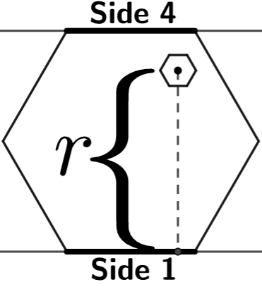
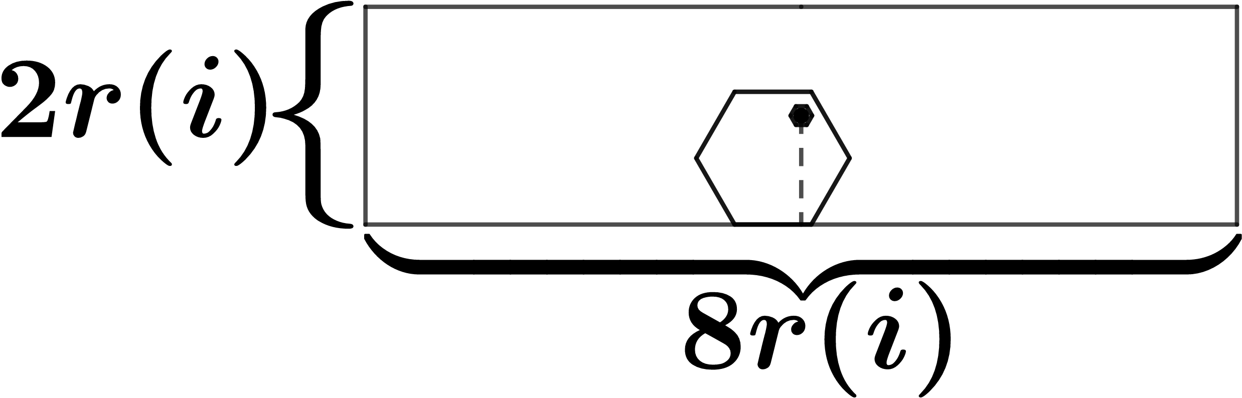
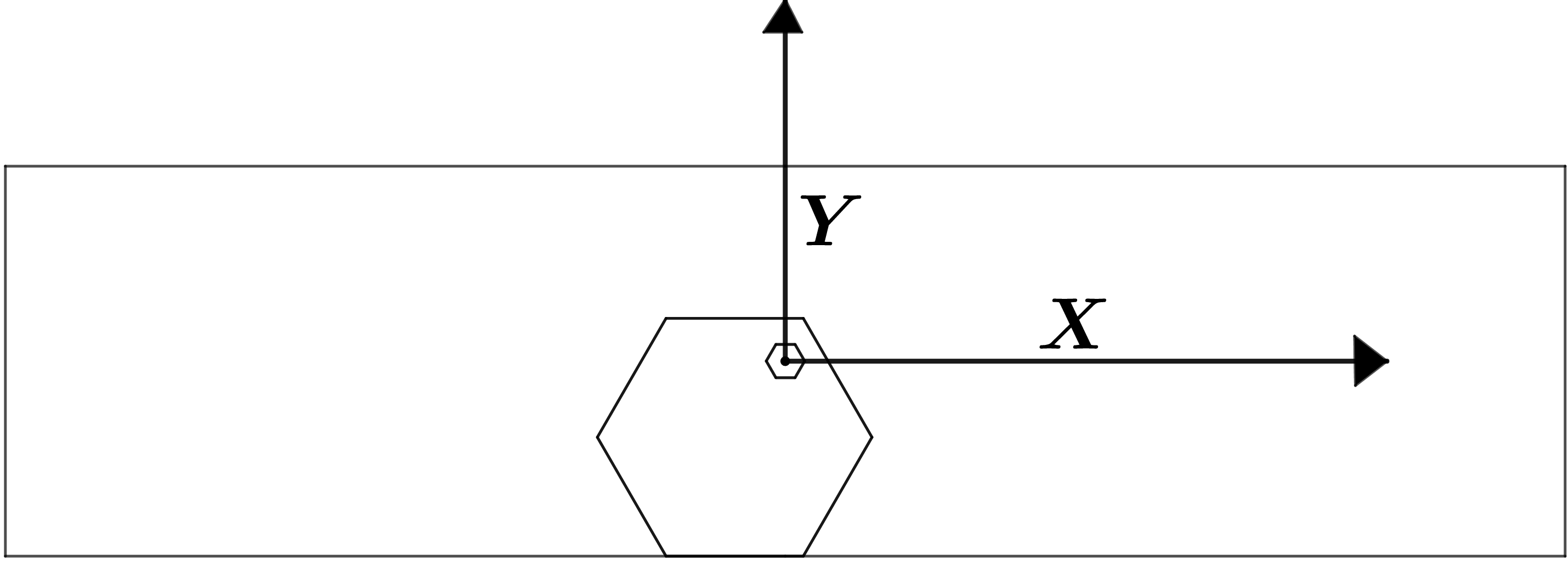
Let $i\in M_{n}$ be a cell (see Figure 2a). Denote by $r(i)$ the maximal distance from the center of the cell $i$ to the lines containing the sides $1$ and $4$ of the hexagon $P$. Denote by $P(i)$ the rectangle $2r(i)\times 8r(i)$ centered at the center of the cell $i$, with the larger side containing one of the side $1$ or $4$ of the hexagon $P$ (See Figure 2b). Without loss of generality we assume that the larger side of the rectangle contains the side $1$ of the hexagon.

Lemma 13.

The hexagon $P$ is entirely contained inside the rectangle $P(i)$.

Proof.

(See Figure 2c). We introduce the Cartesian coordinate system centered at the center of the cell $i$, such that the $x$-axis is parallel to the line containing the side $1$. Then the rectangle $2r(i)\times 8r(i)$ is given by the system

$$\begin{cases}-4r(i)\leqslant x\leqslant 4r(i),\\ -r(i)\leqslant y\leqslant r(i).\end{cases}$$ (3)

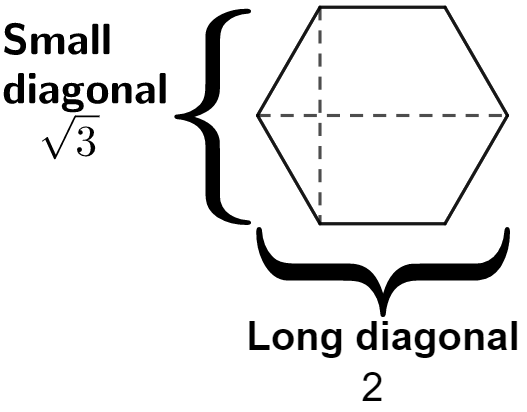
The "long diagonal" (see Figure 2d) of the hexagon $P$ equals $2$, hence the hexagon $P$ is contained inside the rectangle

$$\begin{cases}-2\leqslant x\leqslant 2,\\ -r(i)\leqslant y\leqslant r(i).\end{cases}$$ (4)

The "small diagonal" (see Figure 2d) of the hexagon $P$ equals $\sqrt{3}$, hence $r(i)\geqslant\sqrt{3}/2$. Therefore, if a point $(x,y)$ satisfies system (4), then it also satisfies system (3). ∎

(a)

(b)

(c)

(d)

Figure 2:

To the set $M_{n}$ add all the cells that are entirely contained in the rectangle $P(i)$. Denote by $M^{\prime}_{n}$ the resulting set. In what follows, the colorings of the set $M^{\prime}_{n}$ into 2 colors $\pm 1$ are denoted by points in the set $\{-1,+1\}^{|M^{\prime}_{n}|}$.

Lemma 14.

The following inequalities hold:

$$P(\{x\in\{-1,+1\}^{m}:\text{in the coloring }x\text{ there exists percolation from the cell }i\text{ to the side }1\})\leqslant$$

$$P(\{x\in\{-1,+1\}^{|M^{\prime}_{n}|}:\text{in the coloring }x\text{ there exists percolation from the cell }i\text{ to the side }1\})\leqslant$$

$$P(\{x\in\{-1,+1\}^{|M^{\prime}_{n}|}:\text{in the coloring }x\text{ there exists percolation from the cell }i\text{ to the boundary of }M^{\prime}_{n}\}).$$

Proof.

By Lemma 13 we have $M_{n}\subset M^{\prime}_{n}$. If there exists percolation in the coloring $x\in\{-1,+1\}^{m}$, then there exists percolation in all the colorings $y\in\{-1,+1\}^{|M^{\prime}_{n}|}$ coinciding with the coloring $x$ on the set $M_{n}$. This implies the first inequality.

If in some coloring of the set $M_{n}$ there exists percolation from the cell $i$ to the side $1$, then by Lemma 13 in this coloring there exists percolation from the cell $i$ to a cell of the boundary of the set $M^{\prime}_{n}$. This implies the second inequality. ∎

Lemma 15.

We have

$$\min\{ P(\{x\in\{-1,+1\}^{m}:\text{in the coloring }x\text{ there exists percolation from the cell }i\text{ to the side }1\}),$$

$$P(\{x\in\{-1,+1\}^{m}:\text{in the coloring }x\text{ there exists percolation from the cell }i\text{ to the side }4\})\}\leqslant$$

$$P(\{ \text{in the set }M_{n}\text{ there exists percolation from the cell }O\text{ to the boundary}\}).$$

Proof.

Consider the regular hexagon centered at the center of the cell $i$, obtained from the hexagon $P$ by translation. Since $r(i)~{}\geqslant~{}\sqrt{3}/2$ (see. Figure 2d), it follows that the resulting hexagon is entirely contained inside the rectangle $P(i)$. By Lemma 14 this implies the required inequality. ∎

Proof of Theorem 1.

Theorem 1 follows directly from Corollary 3, Lemmas 11, 12, and 15, and Theorem 2. ∎

4.4 Arguments in favor of Conjecture 3

In conclusion, we give informal arguments in favor of Conjecture 3. In the (degenerate) case when the hexagon $P$ consists of a single cell, we have $\frac{P(A_{1,n}\cap A_{2,n}\cap A_{3,n})}{P(A_{1,n})P(A_{2,n})P(A_{3,n})}=1$. In Example 1, the set $M_{n}$ is larger, and we have $\frac{P(A_{1,n}\cap A_{2,n}\cap A_{3,n})}{P(A_{1,n})P(A_{2,n})P(A_{3,n})}>1$. A natural conjecture is that as the number of the cells in the set $M_{n}$ increases, the ratio in question also increases. We also give the following more solid argument by K. Izyurov.

Consider the following function of a coloring $x\in\{-1,+1\}^{m}$:

$$\chi(x)=\chi(x_{1},\ldots,x_{m})=\begin{cases}\hbox{\multirowsetup 1,}&\text{if in the coloring $x$ there exists percolation between }\\ &\text{the center and the boundary of the set $M_{n}$;}\\ 0,&\text{otherwise.}\end{cases}$$

Now we state a lemma and a corollary. (The proofs are analogous to the proof of Lemma 10.)

Lemma 16.

$P(A_{1,n})=P(A_{2,n})=P(A_{3,n})=\widehat{\chi_{\varnothing}}$ and $P(A_{1,n}\cap A_{2,n}\cap A_{3,n})=~{}\displaystyle{\sum_{S\subset\{1,\ldots,m\}}~{}\widehat{\chi_{S}}^{3}}.$

Corollary 4.

$P(A_{1,n}\cap A_{2,n}\cap A_{3,n})-P(A_{1,n})P(A_{2,n})P(A_{3,n})=\displaystyle{\underset{S\neq\varnothing}{\sum_{S\subset\{1,\ldots,m\}}}\widehat{\chi_{S}}^{3}}.$

Thus Conjectures 2 and 3 are equivalent to the inequalities

$${\underset{S\neq\varnothing}{\sum_{S\subset\{1,\ldots,m\}}}\widehat{\chi_{S}}^{3}}>0\text{ and }\displaystyle{\lim_{n\to+\infty}}{\underset{S\neq\varnothing}{\sum_{S\subset\{1,\ldots,m\}}}\left(\frac{\widehat{\chi_{S}}}{\widehat{\chi_{\varnothing}}}\right)}^{3}>0.$$

The latter sum contains

$$\sum_{\text{$s$ is adjacent to the center $O$}}\left(\frac{\widehat{\chi_{S}}}{\widehat{\chi_{\varnothing}}}\right)^{3}.$$

Consider some cell $i$ among the 6 ones adjacent to the center $O$. The coefficient $\chi_{\{i\}}$ equals the probability that the coordinate $i$ is pivotal. It is easy to prove that the probability that the coordinate $i$ is pivotal conditioned by the existence of percolation (i.e., $\chi_{\{i\}}/\chi_{\varnothing}$) is small, but positive and does not tend to $0$ as $n\to\infty$. Hence, these 6 summands make a contribution that does not disappear in the limit (and the desired limit can be equal to $0$, only if this contribution is canceled with other Fourier-Welsh coefficients, what no reason can be seen for). Since a contribution is small, it is not noticed in numerical experiments.

5 Numerical experiments

In order to verify Conjectures 2-3 about percolation from the center, a computer program was written. (See C++ code in [6].)

Each side of the hexagon $P$ is taken to be parallel to some side of a lattice cell. The program considers $k$ random colorings of the polygon $M_{n}$. Depending on input $p=1,2,$ or $3$, it computes the number $T_{p}$ of colorings with percolation of all the fluids $1,\ldots,p$. (For example, if $p=2$, then the program computes the number of colorings with percolation of both fluids $1$ and $2$.)

Input	Output
$n$	$T_{p}$
$k$
$p$

Output results for some $n$, $k$, and $p$ are shown in Table 2. Additionally, the value $P=(T_{3}/k)/(T_{1}/k)^{3}\approx\frac{P(A_{1,n}\cap A_{2,n}\cap A_{3,n})}{P(A_{1,n})P(A_{2,n})P(A_{3,n})}$ is computed. Presence of values $P<1$ does not disprove Conjecture 2, because it can be caused by statistical deviations. For $n=500,k=1000000,p=1$ the program runs approximately 2 hours.

Table 2: Output results

n	k	$T_{1}$	$T_{2}$	$T_{3}$	$P$	$P-1$
3	10 000 000	9 844 112	9 690 354	9 538 785	1.000	<0.001
4	10 000 000	9 843 390	9 691 475	9 537 528	1.000	<0.001
5	10 000 000	9 655 567	9 327 500	9 009 425	1.001	0.001
6	10 000 000	9 575 758	9 166 785	8 779 321	1.000	<0.001
7	10 000 000	9 478 577	8 985 300	8 522 311	1.001	0.001
8	10 000 000	9 368 765	8 778 158	8 229 285	1.001	0.001
9	10 000 000	9 285 683	8 630 914	8 016 759	1.001	0.001
10	10 000 000	9 211 830	8 475 622	7 813 657	1.000	<0.001
15	10 000 000	8 898 951	7 893 907	7 030 482	0.998	-0.002
20	10 000 000	8 657 067	7 466 236	6 462 095	0.996	-0.004
25	10 000 000	8 461 617	7 166 402	6 016 836	0.993	-0.007
50	1 000 000	787 626	621 883	490 967	1.005	0.005
100	1 000 000	733 994	539 606	395 491	1.000	<0.001
150	1 000 000	707 948	500 289	354 320	0.999	-0.001
200	1 000 000	681 800	466 133	318 058	1.004	0.004
300	1 000 000	660 490	429 462	283 512	0.984	-0.016
400	1 000 000	633 621	402 712	259 337	1.019	0.019
500	1 000 000	621 187	386 527	242 821	1.013	0.013
1500	1 000 000	555 244	299 740	166 587	0.973	-0.027

Let us describe the algorithm checking whether fluid $1$ percolates from the center $O$ to the boundary in a given coloring. Since the color of the center is irrelevant, we may assume that the center has color $0$. (See Table 3 for examples.)

Fix a coloring. At the beginning, a beetle sits at the center. The beetle is allowed to move to an adjacent cell with color $0$ or $1$. We are going to find out if the beetle can reach the boundary.

Step 1. If the beetle is already in a boundary cell, then go to END1. Otherwise go to Step 2.

Step 2. If the color of the cell below the beetle is $0$ or $1$, then move the beetle downwards, and go to Step 1. If the color of the cell below the beetle is $2$ or $3$, then go to Step 3.

Step 3. (Building of a wall; see Table 3)

Construct a finite sequence (called a wall in what follows) of distinct adjacent sides of cells (called wall segments) as follows. The first term of the sequence is the bottom side of the cell where the beetle is located, and the second term of the sequence is adjacent to the left endpoint of the first wall segment. All the cells from one side of the wall have color $0$ or $1$, and all the cells from the other side of the wall have color $2$ or $3$. And finally, either the last wall segment lies between two boundary cells or all the wall segments surround some collection of cells of $M_{n}$. In the former case go to END1 and in the latter case go to Step 4.

(It is easy to see that the wall is uniquely defined by the conditions above.)

Step 4. Draw the ray from the center of $M_{n}$ to the bottom. If the ray intersects with wall segments (which were constructed in Step 3) an odd number of times, then go to END2. Otherwise, move the beetle to the cell right below the lowest wall segment intersecting the ray, and go to Step 1.

END1. There is a percolation from the center to the boundary.

END2. There is no percolation from the center to the boundary.

The following table shows how the algorithm works. In all three examples $n=7$.

Table 3: Percolation-checking algorithm

Example 1
At the beginning, the beetle is sits at the center.	The beetle moves downwards until it hits a blue cell. We put a wall segment right below the beetle.	We build the wall until we put a wall segment between two boundary cells.	The beetle can move along the wall to reach the boundary.
Example 2
At the beginning, the beetle sits at the center.	The beetle moves downwards until it hits a red cell. We put a wall segment right below the beetle.	We build the wall until it encloses some area of $M_{7}$.	We draw the ray from the center to the bottom. The ray intersects a unique wall segment. Hence the beetle cannot reach the boundary.
Example 3
At the beginning, the beetle sits at the center. It cannot move downwards, thus we put a wall segment right below the beetle.	We build a wall until it surrounds some area of $M_{7}$.	We draw the ray from the center to the bottom. The ray intersects two wall segments.	The beetle gets around the wall. Afterwards, it moves down and reaches the boundary.

6 Acknowledgements

The author is grateful to his research advisor M. Skopenkov for setting the problems and constant attention to this work; to K. Izyurov, A. Magazinov, and M. Khristoforov for reading this work and sending valuable comments; to K. Izyurov and A. Magazinov for telling the proof of Theorem 1.

References

- [1] R. O’Donnell. Analysis of Boolean functions. Cambridge University Press, New York, 2014.
- [2] H. Kesten, Percolation theory for mathematicians, Birkhuser, Boston, 1982.
- [3] H. Duminil-Copin, Introduction to Bernoulli percolation, 2018, https://www.ihes.fr/~duminil/publi/2017percolation.pdf.
- [4] G. Grimmet, Percolation (2. ed). Springer Verlag, 1999.
- [5] A. Yadin, Percolation, 2013, https://www.math.bgu.ac.il/~yadina/percolation.pdf.
- [6] I. Novikov, A software to compute probability, https://github.com/IVNov/percolation-in-hexagonal-lattice/blob/master/PPercolation.cpp.