HAMNER: Headword Amplified Multi-span Distantly Supervised Method for Domain Specific Named Entity Recognition

Abstract

To tackle Named Entity Recognition (NER) tasks, supervised methods need to obtain sufficient cleanly annotated data, which is labor and time consuming. On the contrary, distantly supervised methods acquire automatically annotated data using dictionaries to alleviate this requirement. Unfortunately, dictionaries hinder the effectiveness of distantly supervised methods for NER due to its limited coverage, especially in specific domains. In this paper, we aim at the limitations of the dictionary usage and mention boundary detection. We generalize the distant supervision by extending the dictionary with headword based non-exact matching. We apply a function to better weight the matched entity mentions. We propose a span-level model, which classifies all the possible spans then infers the selected spans with a proposed dynamic programming algorithm. Experiments on all three benchmark datasets demonstrate that our method outperforms previous state-of-the-art distantly supervised methods.

1 Introduction

Named entity recognition (NER) is a task that extracts entity mentions from sentences and classifies them into pre-defined types, such as person, location, disease, chemical, etc. It is a vital task in natural language processing (NLP), which benefits many downstream applications including relation extraction (?), event extraction (?), and co-reference resolution (?).

With a sufficient amount of cleanly annotated texts (i.e., the training data), supervised methods (?; ?) have shown their ability to achieve high-quality performance in general domain NER tasks and benchmarks. However, obtaining cleanly annotated texts is labor-intensive and time-consuming, especially in specific domains, such as the biomedical domain and the technical domain. This hinders the usage of supervised methods in real-world applications.

Distantly supervised methods circumvent the above issue by generating pseudo annotations according to domain specific dictionaries. Dictionary is a collection of $\langle{\text{{entity mention}, {entity type}}}\rangle$ pairs. Distantly supervised methods firstly find entity mentions by exact string matching (?; ?) or regular expression matching (?) with the dictionary, and then assign corresponding types to the mentions. A model is trained on the training corpus with the pseudo annotations. As the result, distant supervision significantly reduces the annotation cost, while not surprisingly, the accuracy (e.g., precision and recall) reduces.

In this paper, we aim to reduce the gap between distantly supervised methods and supervised methods. We observed two limitations in distantly supervised methods. The first limitation is that the information in the dictionary has not been fully mined and used. For example, consider a newly discovered disease namely ROSAH syndrome, which is unlikely to exist in the dictionaries, and hence cannot be correctly extracted and annotated if we use simple surface matching. However, human beings can easily recognize it as a disease, since there are many disease entity mentions in the dictionaries that are ended with syndrome. This motivates us to use headwords of entity mentions as indicators of entity types, and thus improves the quality of the pseudo annotations.

The second limitation in distantly supervised methods is that most of the errors come from incorrect boundaries. Most methods (including supervised methods) model the NER problem as a sequence labeling task and use popular architectures/classifiers like BiLSTM-CRF (?). However, CRFs suffer from sparse boundary tags (?), and pseudo annotations can only be more sparse and noisy. In addition, CRFs focus more on word-level information and thus cannot make full use of span-level information (?). Some methods choose to fix the entity boundaries before predict the entity type. Apparently, any incorrect boundary will definitely lead to incorrect output, no matter how accurate the subsequent classifier is. Therefore, we propose to decide entity boundaries after predicting entity types. As such, there would be more information, such as the types and confidence scores of entity mentions, which can help to determine more accurate entity boundaries.

Based on the above two ideas, we propose a new distantly supervised method named HAMNER (Headword Amplified Multi-span NER) for NER tasks in specific domains. We first introduce a novel dictionary extension method based on the semantic matching of headwords. To account for the possible noise introduced by the extended entity mentions, we also use the similarity between the headwords of the extended entity mentions and the original entity mentions to represent the quality of the extended entity mentions. The extended dictionary will be used to generate pseudo annotations. We then train a model to estimate the type of a given span from a sentence based on its contextual information. Given a sentence, HAMNER uses the trained model to predict types of all the possible spans subject to the pre-defined maximum number of words, and uses a dynamic programming based inference algorithm to select the most proper boundaries and types of entity mentions while suppressing overlapping and spurious entity mentions.

The main contributions of this paper are

• We generalize the distant supervision idea for NER by extending the dictionaries using semantic matching of headwords. Our extension is grounded in linguistic and distributional semantics. We use the extended dictionary to improve the quality of the pseudo annotations.

• We propose a span-level model with both span information and contextual information to predict the type for a given span. We propose a dynamic programming inference algorithm to select the spans which are the most likely to be entity mentions.

• Experiments on three benchmark datasets have demonstrated that HAMNER achieves the best performance with dictionaries only and no human efforts. Detailed analysis has shown the effectiveness of our designed method.

2 Related Work

Named entity recognition (NER) attracts researchers and has been tackled by both supervised and semi-supervised methods. Supervised methods, including feature based methods (?; ?; ?) and neural network based methods (?; ?; ?), require cleanly annotated texts. Semi-supervised methods either utilize more unlabeled data (?) or generate annotated data gradually (?; ?; ?).

Distant supervision is proposed to alleviate human efforts in data annotation (?; ?). ? ? propose distant supervision to handle the limitation of human annotated data for relation extraction task (?). They use Freebase (?), instead of human, to generate training data with heuristic matching rules. For each pair of entity mentions with some Freebase relations, sentences with these entity mentions are regarded as sentences with such relations. Beyond the heuristic matching rules, ? ? learn a matching function with a small amount of manually annotated data (?).

Recently, distant supervision has been explored for NER tasks (?; ?; ?). SwellShark (?) utilizes a collection of dictionaries, ontologies, and, optionally, heuristic rules to generate annotations and predict entity mentions in the biomedical domain without human annotated data. ? ? use exact string matching to generate pseudo annotated data, and apply high-quality phrases (i.e., mined in the same domain without assigning any entity types) to reduce the number for false negative annotations (?). However, their annotation quality is limited by the coverage of the dictionary, which leads to a relatively low recall. In the technical domain, Distant-LSTM-CRF (?) applies syntactic rules and pruned high-quality phrases to generate pseudo annotated data for distant supervision. The major differences between HAMNER and other distantly supervised methods are 1. HAMNERextended the coverage of dictionaries without human efforts. 2. HAMNERmakes predictions in the span level with both entity type and boundary information.

3 Problem Definition

We represent a sentence as a word sequence $(x_{1},x_{2},\ldots,x_{N})$. For span $(x_{i},\ldots,x_{j})$ from the sentence, we use $\langle i,j\rangle$ to denote its boundaries, and use $l\in L$ to denote its type, where $L$ represents the list of pre-defined types (e.g., Disease, Chemical) and none type (e.g., None). We let None be the last element in $L$ (i.e., $L_{|L|}$).

We tackle the problem with distant supervision. Unlike supervised and semi-supervised methods, we require no human annotated training data. Instead, we only require a dictionary as the input in addition to the raw text. The dictionary is a collection of $\langle$entity mention, entity type$\rangle$-tuples. We use dictionary in the training phase to help generate pseudo annotations on the training corpus.

We argue that dictionaries are easy to obtain, either from publicly available resources, such as Freebase (?) and SNOMED Clinical Terms, or by crawling terms from some domain-specific high-quality websites .

4 The Proposed Method

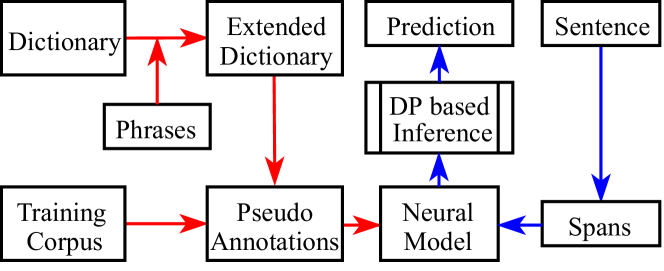
Figure 1: The process of the proposed method. Red arrows show the training steps, including dictionary extension, pseudo annotation generation, and model training. Blue arrows show the prediction phases, including span generation, model prediction, and dynamic programming (DP) based inference.

Figure 1 illustrates the key steps in HAMNER. In training, our method firstly generates pseudo annotations according to a headword-based extended dictionary (details in Section 4.1). Then a neural model is trained using the pseudo annotated data. The model takes a span and its context in the sentence as input, and predicts the type of the span. The structure of the neural model is introduced in Section 4.2.

Prediction is performed in two phases. Given a sentence, in phase one, we generate all the possible spans whose length is no more than a specified threshold, and use the trained neural model to predict the types of these spans. In phase two, we apply a dynamic programming based inference algorithm to determine the entity mentions and their types. The details are presented in Section 4.3.

Unlike previous works (?; ?), we solve NER in span-level where information has not been fully explored. HAMNER is based on all the possible spans up to a certain length instead of only considering those based on the prediction of a model (?). While this is an effective solution for purely supervised methods in semantic role labeling (SRL) (?) and nested/non-overlap NER (?; ?), we are the first to apply this to distantly supervised NER. Specifically, we generate all the spans $\langle i,j\rangle$ containing up to $M$ words as candidate spans, where $M$ is a pre-defined parameter. Therefore, a sentence with $N$ words will generate $\frac{M(2N-M+1)}{2}$ spans, which is still linear in the length of the sentence.

4.1 Generating Pseudo Annotations

In this section, we aim to improve the quality of the pseudo annotations. While most of the existing distantly supervised methods use domain specific dictionaries to annotate texts, we find that they are struggling because of the following two cases.

• Out-of-dictionary entity mentions. It is common that the dictionaries are not frequently updated. However, new entities and concepts are generated everyday. Therefore, the coverage of a dictionary is generally not high.

• Synonyms and spelling differences. Most dictionaries may not contain both terms in a pair of synonyms. And they usually stick with one spelling form (e.g., British or American spelling). Both of these cases can enrich the annotations thus should not be ignored.

Therefore, we propose to extend the dictionary by adding a set of domain specific high-quality phrases. The high-quality phrases can be obtained in multiple ways. For example, we can use an unsupervised phrase mining methods (?; ?; ?; ?) on a large corpus in the same domain, or collect unclassified terms from lexicon resources, such as mediLexicon .

However, these phrases do not have types. To assign types to these high-quality phrases, we propose to make use of headwords. It is well-known that headwords of entity mentions play an important role in information extraction tasks (?). In a similar vein, the headword of a noun phrase is usually highly indicative of the type of noun phrase. For example, appendix cancer shares the same headword cancer with liver cancer; hence, if we know that the type of the former is Disease, then we can infer that the type of the latter is probably the same.

We also consider non-exact string matching on the headwords to deal with synonyms and spelling differences. Our idea is based on the hypothesis that similar words tend to occur in similar contexts (?) and hence may have a high probability of belonging to the same type. Thanks to word embedding methods, we can measure such distributional similarity based on the cosine similarity between the corresponding word embeddings. For example, since the word embeddings of tumor and tumour are close, their types should be the same.

1

Input : Dictionary $D$, High-quality Phrase Set $P$, headword frequency threshold $\tau_{1}$, headword similarity threshold $\tau_{2}$

Output : Extended Dictionary $D_{ext}$

2 $H\leftarrow$ set of headwords that occurs more than $\tau_{1}$ times in D;

3$D_{ext}\leftarrow\emptyset$;

4for each $p\in P$ do

       /* $s$: the max cosine similarity */

       /* $T$: the set of types */

5      $s\leftarrow 0$;

6      $T\leftarrow\emptyset$;

7      for each $\langle e_{i},t_{i}\rangle\in D$ do

8             if $hw(e_{i})\in H\wedge sim(hw(p),hw(e_{i}))\geq\tau_{2}$ then

9                   if $sim(hw(p),hw(e_{i}))>s$ then

10                         $s\leftarrow sim(hw(p),hw(e_{i}))$;

11                        $T\leftarrow\{t_{i}\}$;

12                  else if $sim(hw(p),hw(e_{i}))=s$ then

13                         $T\leftarrow T\cup\{t_{i}\}$;

14                  

15            

16      for each $t\in T$ do

17             $D_{ext}=D_{ext}\cup\{(p,t,s)\}$;

18      

19for each $\langle e_{i},t_{i}\rangle\in D$ do

20       $D_{ext}=D_{ext}\cup\{(e_{i},t_{i},1)\}$;

return $D_{ext}$

Algorithm 1 Dictionary Extension

Algorithm 1 presents the procedure of dictionary extension in HAMNER, where $hw(x)$ is the headword of the phrase/entity $x$, and $sim(x,y)$ is the cosine similarity between the word embeddings of $x$ and $y$. We have noticed that while the word embedding based non-exact string matching improves the coverage of the dictionary, it also brings some noise. Therefore, we use $\tau_{1}$ to prune those infrequent headwords (i.e., Line 1), and use $\tau_{2}$ to avoid matching with dissimilar headwords (i.e., Line 1). We also only keep the types with the highest cosine similarity (i.e., Line 1-1).

Through Algorithm 1 we obtain a large set of entity mentions, along with their types and the cosine similarities. We then annotate the unlabeled data via exact string matching of the entity mentions. We follow the existing work that favors longest matching entity mentions, hence we sort the entity mentions in the dictionary by their length, and start matching the spans in the sentences greedily from the longest one. We do not allow the annotations to be nested or overlapping. But we do allow one span to have multiple types as two entities of different types may share the same entity mention in the dictionary.

In addition to the types, we also assign a weight to each annotation. Assume that a span is matched by an entity mention in the extended dictionary with pre-defined type $l$ and the corresponding cosine similarity $s$. While we set annotation weight 1 for entity mentions themselves or their headwords appearing in the original dictionary, we use a proposed $\mathrm{sigmoid}$ function to control the noise introduced by non-exact matched entity mentions. Thus, we define the annotation weight $w_{l}$ for type $l$ using the function as follows,

$$w_{l}=\begin{cases}\mathrm{sigmoid}(\theta_{1}\cdot s+\theta_{2}),&\text{if s $<$ 1}.\\ 1,&\text{if s $=$ 1}.\end{cases}$$ (1)

, where $\theta_{1}$ and $\theta_{2}$ are hyper-parameters. The annotation weight can be interpreted as a confidence score of the annotation and will be used in the neural model in Section 4.2.

For each span, we use $\langle i,j\rangle$ to indicate its boundaries in the sentence, and hence it will be represented as $(\langle i,j\rangle,w_{L_{1}},\dots,w_{L_{|L|}})$. If a span is annotated with pre-defined types, then we use Equation (1) to compute the weights for the corresponding annotated types, while setting weights to 0 for the rest types. Otherwise, only $w_{L_{|L|}}$ (i.e. weight of None type) is set to 1 while the rest weights set to 0. These two types of spans will serve as positive and negative samples during training.

4.2 Modelling Type Distribution of Spans

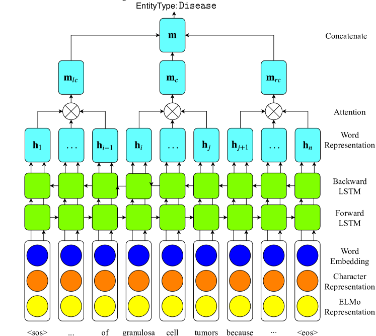
Figure 2: Overview of the neural model. The example shows the span (i.e., granulosa cell tumors) and the corresponding context. This span is annotated as Disease during preprocessing mentioned in Section 4.1. Words $\langle sos\rangle$ (start of a sentence) and $\langle eos\rangle$ (end of a sentence) are added in each sentence to construct contexts for spans at the start and at the end of a sentence.

We design a novel neural network model to model the type distribution of given spans, i.e., given any span $\langle{i,j}\rangle$, the model will predict $p(l\mid\langle{i,j}\rangle$) for all types $l\in L$. Our model exploits typographical, semantics, and contextual features, and employs a new loss function to deal with multiple weighted annotated types. The architecture of our proposed neural model is shown in Figure 2.

Word Representation

To extract morphological information, such as prefixes and suffixes of a word, we use CNN to encode the character representation following (?). We also apply pre-trained ELMo (?) for the contextualized word representation.

We then concatenate the pre-trained word embedding, ELMo word representation and character representation for each word, and feed them into the Bidirectional LSTM layer (?). The outputs of both directions are concatenated together and form the word representations $[\mathbf{h}_{1},\mathbf{h}_{2},\ldots,\mathbf{h}_{n}]$.

Context-Sensitive span representation

Given a span $c=\langle i,j\rangle$, it separates the sentence into three parts and we can get their corresponding hidden representations from the BiLSTM layer as: (1) the left context of the span $\mathbf{H}_{\text{lc}}=[\mathbf{h}_{1},\ldots,\mathbf{h}_{i-1}]$; (2) the inner content of the span $\mathbf{H}_{\text{c}}=[\mathbf{h}_{i},\ldots,\mathbf{h}_{j}]$; and (3) the right context of the span $\mathbf{H}_{\text{rc}}=[\mathbf{h}_{j+1},\ldots,\mathbf{h}_{n}]$.

To obtain a fixed representation for any of $\mathbf{H}_{z}$ ($z=\{\text{lc},\text{c},\text{rc}\}$), we adopt the self-attention mechanism (?). Specifically, we calculate the attention vector, $\mathbf{a}_{z}$ over the variable-length input $\mathbf{H}_{z}$, and then obtain the weighted hidden state $\mathbf{m}_{z}$ as $\mathbf{m}_{z}=\mathbf{H}_{z}\mathbf{a}^{\top}_{z}$, where $\mathbf{a}_{z}=\textsf{Softmax}(\mathbf{w}_{z}^{\top}\tanh(\mathbf{W}\mathbf{H}_{z}))$. Finally, we obtain the final representation $\mathbf{m}$ by concatenating $\mathbf{m}_{\text{lc}}$, $\mathbf{m}_{\text{c}}$, and $\mathbf{m}_{\text{rc}}$ together.

Loss function

Given the final span representation $\mathbf{m}$, we multiply it with the type embedding $\mathbf{l}$ of $l\in L$, and obtain the probability distribution over all types via the Softmax function:

$$p(l\mid\mathbf{m})=\frac{\exp(\mathbf{l}^{\top}\mathbf{m})}{\sum_{\tilde{\mathbf{l}}\in L}\exp(\tilde{\mathbf{l}}^{\top}\mathbf{m})},$$ (2)

The type embeddings $\mathbf{l}$ will be part of the parameters of the model.

As one span can be annotated with multiple pre-defined types $l$ in $L$ and the corresponding weight $w$, we modify the cross-entropy loss to take these into consideration. The loss function $J$ is defined as $J=-\sum_{c\in C}\left(\sum_{l\in L}w_{l}\cdot\log(p(l\mid\mathbf{m}))\right)$, where $C$ indicates all the candidate spans, $w_{l}$ indicates the annotation weight of type $l$ mentioned in Section 4.1.

4.3 Inference

Our neural network based model provides probability estimation for all the candidate spans and all the types, we need to perform two tasks in the inference process: (1) find a non-overlapping span partition of the sentence, and (2) assign a type to each span. The second step is straightforward, as we just assign the type with the largest probability predicted by the model. Hence, we mainly focus on the first step below.

We model this problem as an optimization problem, where the goal is to find a non-overlapping span partition such that the joint probability of each span being None type is minimized. The intuition is that we want to encourage the algorithm to find more entity mentions of types other than None, hence increasing the recall of the method. More specifically, our objective function is:

$$\operatorname*{arg\,min}\limits_{V\in\mathcal{V}}\sum_{c\in V}\log(p(\text{{None}}\mid c)),$$

where each $V$ is a partitioning of the sentence into a set of disjoint and complete spans $[c_{1},c_{2},\ldots]$, and $\mathcal{V}$ is all the possible partitionings.

1

Input : Candidate set $U$, sentence length $N$

Output : Sentence $S$ with labeled spans

2 $r[0]\leftarrow 0$;

3for $j=1$ to $N$ do

4       $r[j]\leftarrow\min_{1\leq i\leq j}(r[i-1]+\log(p(\text{{None}}|\langle i,j\rangle))$;

5$V\leftarrow\mathsf{construct\_partitioning}(r)$;

6$S\leftarrow\mathsf{label\_spans}(V)$;

return $S$

Algorithm 2 DP Based Inference

A naive optimization algorithm is to enumerate all possible partitionings and compute the objective function. It is extremely costly as there are $O(2^{N})$ such partitionings ($N$ is the length of the sentence). In contrast, we propose a dynamic programming algorithm, whose time complexity is only $O(NM)$ ($M$ is the maximal number of words in a span), to find the optimal partitioning. As shown in Algorithm 2, where candidate set $U$ stores all spans and the predicted probability of the types, we use $r[j]$ to store the minimum log probability of the first $j$ tokens in the sentence. We sequentially update $r[j]$ where $j$ increases from $1$ to $N$. Note that $p(\text{{None}}\mid\langle{i,j}\rangle)$ can be computed in our model by computing the corresponding $\mathbf{m}$ for the span $\langle{i,j}\rangle$ and Equation (2).

Once we obtained $r[N]$, we backtrack and reconstruct the optimal partitioning (i.e., $\mathsf{construct\_partitions}$), and assign each span the type with the highest probability (i.e., $\mathsf{label\_spans}$).

5 Experiments

In this section, we evaluate our method and compare it with other supervised and distantly supervised methods on three benchmark datasets. In addition, we investigate the effectiveness of the designed method with a detailed analysis.

5.1 Experiment Setting

Datasets

An overview of the datasets and dictionaries is shown in Table 1.

Table 1: Dataset overview

Dataset	BC5CDR	NCBI-Disease	LaptopReview
Domain	Biomedical	Biomedical	Technical Review
Entity Types	Disease, Chemical	Disease	AspectTerm
Dictionary	MeSH + CTD	MeSH + CTD	Computer Terms

Table 2: NER performance comparison. The bold-faced scores represent the best results among distantly supervised methods.

Method	Human Effort	BC5CDR			NCBI-Disease			LaptopReview
	other than Dictionary	Pre	Rec	$F_{1}$	Pre	Rec	$F_{1}$	Pre	Rec	$F_{1}$
Supervised model	Gold Annotations	88.17	88.39	88.28	85.34	90.94	88.05	85.14	80.58	82.80
SwellShark	Regex Design + Case Tuning	86.11	82.39	84.21	81.6	80.1	80.8	-	-	-
	Regex Design	84.98	83.49	84.23	64.7	69.7	67.1	-	-	-
Dictionary Match	None	93.93	58.35	71.98	90.59	56.15	69.32	90.68	44.65	59.84
AutoNER*		83.08	82.16	82.70	76.98	74.65	75.78	68.72	59.39	63.70
HAMNER		86.01	86.34	86.17	82.03	83.56	82.79	74.02	62.02	67.46

BC5CDR dataset (?) consists of 1,500 PubMed articles, which has been separated into training set (500), development set (500), and test set (500). The dataset contains 15,935 Chemical and 12,852 Disease mentions.

NCBI-Disease dataset (?) consists of 793 PubMed abstracts, which has been separated into training set (593), development set (100), and test set (100). The dataset contains 6,881 Disease mentions.

LaptopReview dataset (?) refers to Subtask 1 for laptop aspect term (e.g., disk drive) recognition. It consists of 3,845 review sentences, which contains 3,012 AspectTerm mentions. Following previous work (?), we separated them into training set (2445), development set (609) and test set (800).

Dictionary and High-Quality Phrase

To fairly compare with previous methods, we construct and process dictionaries and high quality phases in the same way as in (?). For the BC5CDR and NCBI-Disease datasets, we combine the MeSH database  and the CTD Chemical and Disease vocabularies  as the dictionary. The phrases are mined from titles and abstracts of PubMed papers using the phrase mining method proposed in (?).

For the LaptopReview dataset, we crawl dictionary terms from the public website . The phrases are mined from the Amazon laptop review dataset using the same phrase mining method.

As suggested in (?), we apply tailored dictionaries to reduce false positive matching.

Headword

We use rule based method proposed in (?) to extract the headwords of phrases. The headword of a phrase is generally the last word of the phrase. If there is a preposition in the phrase, the headword is the last word before the preposition. For example, the headword of the phrase cancer of the liver is cancer.

Metric

Following the standard setting, we evaluate the methods using micro-averaged $F_{1}$ score and also report the precision (Pre) and recall (Rec) in percentage. All the reported scores are averaged over five different runs.

5.2 Implementation

We use the same word embeddings for the neural model and the cosine similarity mentioned in Section 4.1. For the BC5CDR and NCBI-Disease datasets, we use pre-trained 200-dimensional word embeddings (?) and ELMo trained on a PubMed corpus. For the LaptopReview dataset, we use pre-trained 100-dimensional GloVe word embeddings (?) and ELMo trained on a news corpus. We select hyper-parameters that achieve the best performance on the development sets. Details of hyper-parameters of dictionary extension, neural model, and training process are listed in the appendix.

5.3 Compared Methods

We compare HAMNER with other methods from three different categories: supervised model, distantly supervised method with human effort, and distantly supervised method without human effort.

Supervised model. We use supervised model to demonstrate the competitiveness of HAMNER. We use the state-of-the-art model architecture proposed in (?) with ELMo trained in the corresponding domains.

SwellShark (?) is a distantly supervised method designed for the biomedical domain, especially on the BC5CDR and NCBI-Disease datasets. It requires human efforts to customize regular expression rules and hand-tune candidates.

AutoNER (?) is the previous state-of-the-art distantly supervised method without human efforts on all the datasets. Similar to our method, it only requires domain specific dictionaries and a set of high-quality phrases. To make a fair comparison with HAMNER, we have re-implemented AutoNER to add ELMo as part of input representation, which brings the performance improvement.

AutoNER is originally trained with all the raw texts from the dataset (i.e., the training corpus is the union of the training set, development set, and test set). To make a fair comparison with all other methods, we have re-trained AutoNER with raw texts only from the training set. This brings a lower performance than those in the original paper.

Therefore, we use AutoNER* for AutoNER with ELMo and trained on the training set only, and report the evaluation results of AutoNER* in our paper. The readers are referred to (?) for the original performance of AutoNER. Nevertheless, we have tried to train AutoNER with ELMo and using all the raw texts, and the performance is still lower than HAMNER.

We also include purely dictionary match method. We directly apply the original dictionaries to the test sets and get entity mentions and the types by exact string matching.

5.4 Overall Performance

Table 2 shows the performance of different methods on all the datasets. HAMNER achieves the best recall and $F_{1}$ among all the distantly supervised methods. It surpasses SwellShark by around 2% $F_{1}$ score on the BC5CDR and NCBI-Disease datasets, though SwellShark is specially designed for the biomedical domain and needs human efforts.

Purely dictionary matching method achieves the highest precision among all the methods, which is not surprising as dictionaries always contain accurate entity mentions. However, it suffers from low recall which is due to the low coverage of the dictionary and the strict matching rule.

On the contrary, the success of HAMNER owes to the ability of generalization on the out-of-dictionary entity mentions without losing prediction accuracy. As the result, HAMNER achieves significant improvement over the previous state-of-the-art method (i.e., AutoNER*) on both precision and recall. The $F_{1}$ scores are improved by 3.47%, 7.01%, and 3.76% on the three datasets, respectively.

Detailed analysis is shown in the following sections.

5.5 Effectiveness of Dictionary Extension

Table 3: Effectiveness of each component. We do not apply annotation weights on AutoNER* as it does not support weighted annotations.

Component	BC5CDR			NCBI-Disease			LaptopReview
	Pre	Rec	$F_{1}$	Pre	Rec	$F_{1}$	Pre	Rec	$F_{1}$
Neural Model	83.28	83.80	83.54	79.55	76.56	78.02	69.74	57.16	62.78
Neural Model+Dictionary Extension	83.04	85.07	84.04	80.13	81.81	80.95	69.39	59.42	64.00
Neural Model+ELMo	85.98	85.95	85.97	79.91	80.25	80.08	71.78	59.82	65.22
Neural Model+Dictionary Extension+ELMo	86.01	86.34	86.17	82.03	83.56	82.79	74.02	62.02	67.46
AutoNER*+Dictionary Extension	81.53	83.03	82.28	80.12	83.02	81.54	69.61	59.45	64.11

We explore the effectiveness of dictionary extension proposed in Section 4.1. We use precision and recall to evaluate the accuracy and the coverage of annotations on the training set. As shown in Table 4, using the extended dictionary is able to boost the recall (coverage) by a large margin (e.g., on the BC5CDR and NCBI-Disease datasets, the recall increases by more than 20%), while slightly reducing the precision (which is inevitable due to the additional noise introduced by the extended dictionary terms).

Table 4: Annotation quality on the training set.

	BC5CDR		NCBI-Disease		LaptopReview
	Pre	Rec	Pre	Rec	Pre	Rec
Dictionary	94.92	72.23	93.88	60.56	89.01	51.65
Extended Dictionary	91.89	84.48	92.61	83.01	87.73	54.51

Table 5: Effectiveness of weighted annotations.

Method		BC5CDR			NCBI-Disease			LaptopReview
		Pre	Rec	$F_{1}$	Pre	Rec	$F_{1}$	Pre	Rec	$F_{1}$
HAMNER	with weight	86.01	86.34	86.17	82.03	83.56	82.79	74.02	62.02	67.46
	without weight	85.46	86.78	86.12	80.63	83.94	82.24	74.02	62.02	67.46

The increasing of recall on the LaptopReview dataset is not as significant as those on the other two datasets. This is due to the impact of the similarity threshold mentioned in Section 4.1. On the LaptopReview dataset, we use a higher similarity threshold to avoid introducing too much noise to the extended dictionary, which brings less improvement to the coverage of the extended dictionary.

We also investigate the effectiveness of the weight function (i.e. Equation (1)) in the loss function. We assign all annotations with weight 1 to eliminate the effect of the weight function (noted as HAMNER without weight), and show the results in Table 5. It can be seen that the weight function helps HAMNER achieve better precision (e.g. 0.55% and 1.4% improvement on the BC5CDR and NCBI-Disease datasets, respectively) with slightly decrease of recall.

The reason why we have not observed the improvement on the LaptopReview dataset is that we set a higher similarity threshold. We observe the same trend as the other two datasets when we set a lower similarity threshold.

5.6 Effectiveness of Model

To demonstrate the effectiveness of each component in the neural model, we conduct experiments by disabling different components in the model on all the datasets. From the results in Table 3, we observe that each component improves the model from different aspects.

It is worth mentioning that even without using ELMo or the extended dictionaries, the neural model still shows competitive performance compared with AutoNER* which extracts mention boundaries and then predicts the types. This reveals that the span-level modeling and the inference algorithm is more suitable for the NER task compared with the pipeline design.

Dictionary extension improves the coverage of the pseudo annotations, hence boosts the coverage of predictions (i.e. recall). In addition, dictionary extension will not bring in many false-positive predictions, hence will not affect precision. For example, on the NCBI-Disease dataset, dictionary extension improves the precision and recall by 0.58% and 5.25%, respectively.

Table 6: Comparison of $F_{1}$ scores on in-dictionary (ID) and out-of-dictionary (OOD) entity mentions.

		BC5CDR		NCBI-Disease		LaptopReview
		ID	OOD	ID	OOD	ID	OOD
the number of entity mentions		5734	3991	539	416	292	362
$F_{1}$	HAMNER	93.53	76.05	91.96	70.32	92.86	45.51
	AutoNER*	92.80	66.41	91.88	54.05	89.23	37.64

On the other hand, ELMo focuses on the accuracy of predictions. For example, the precision increases from 83.28 % to 85.98 % on the BC5CDR dataset. ELMo also encourages the model to extract more entity mentions.

With both components, HAMNER achieves the best overall performance. It seems that the improvement from dictionary extension and ELMo are additive, which implies that dictionary extension and ELMo improve the model from different aspects.

In order to show the effectiveness of dictionary extension to other models, as well as to show the effectiveness of our proposed framework, we apply the extended dictionaries in AutoNER*. We observe that the performance of AutoNER* improves with the extended dictionaries, however, it is still much lower than our proposed method HAMNER.

5.7 Generalization on OOD Entity Mentions

We perform analysis on the test set for the out-of-dictionary entity mentions to investigate the generalization of HAMNER. Specifically, we partition entity mentions into two subsets: in-dictionary (ID) entity mentions and out-of-dictionary (OOD) entity mentions. An entity mention is considered as an ID mention if it is fully or partially appearing in the dictionary, and an OOD mention otherwise.

Table 6 shows the performance of HAMNER and AutoNER* on the OOD and ID entity mentions. HAMNER surpasses AutoNER* on the ID entity mentions, and it also shows significant improvement on the OOD entity mentions over all the datasets. For example, on the NCBI-Disease dataset, it boosts the $F_{1}$ score by at least 16% on the OOD entity mentions. This explains why HAMNER has a higher overall performance and also demonstrates the stronger generalization ability of HAMNER.

6 Conclusion

In this paper, we presented a new method to tackle NER tasks in specific domains using distant supervision. Our method exploits several ideas including headword-based dictionary extension, span-level neural model, and dynamic programming inference. Experiments show HAMNER significantly outperforms the previous state-of-the-art methods.

Acknowledgement

This work is supported by ARC DPs 170103710 and 180103411, D2DCRC DC25002 and DC25003, NSFC under grant No. 61872446 and PNSF of Hunan under grant No. 2019JJ20024. The Titan V used for this research was donated by the NVIDIA Corporation.

A Appendix

To help readers reproduce the results, we represent the details for implementing our proposed method. In this section, we list details of hyper-parameter for dictionary extension, neural model construction, and training.

A.1 Dictionary Extension Hyper-parameters

Table 7 lists the hyper-parameters for dictionary extension. In the biomedical domain, we set headword threshold $\tau_{\text{1}}$ to 5 and similarity threshold $\tau_{\text{2}}$ to 0.4. In the technical review domain, we set headword threshold $\tau_{\text{1}}$ to 3 and similarity threshold $\tau_{\text{2}}$ to 0.9. This controls the possible noise introduced by the extended dictionary terms. For the weight function, we set $\theta_{1}$ to 1.0 and $\theta_{2}$ to -0.5 in both domains.

Table 7: Dictionary Extension Hyper-parameters

Domain	Biomedical	Technical Review
headword frequency threshold $\tau_{\text{1}}$	5	3
similarity threshold $\tau_{\text{2}}$	0.4	0.9
label weight $\theta_{1}$	1.0
label weight $\theta_{2}$	-0.5

A.2 Neural Model Hyper-parameters

Table 8 lists the hyper-parameters for the neural model. Character embeddings are initialized with uniform samples from $[-\sqrt{\frac{3}{d}},+\sqrt{\frac{3}{d}}]$, with $d$ is set to 16. We apply CNNs with kernel sizes 2,3,4 to fully explore the morphological information in the biomedical domain. In the technical review domain, we use CNNs with kernel size 3. For the BC5CDR and NCBI-Disease datasets, we use pre-trained 200-dimensional word embeddings (?) and ELMo trained on a PubMed corpus. For the LaptopReview dataset, we use pre-trained 100-dimensional GloVe word embeddings (?) and ELMo trained on a news corpus. We use a single-layer Bidirectional LSTM (BiLSTM) (?) with the hidden state dimension of the BiLSTM set to 256.

Table 8: Neural Model Hyper-parameters

Domain		Biomedical	Technical Review
Char-level Embedding	dimension	16
CNN	kernel size	2,3,4	3
	padding	1,2,3	2
	stride	1,1,1	1
	channel	128,128,128	128
Word-level Embedding	dimension	200	100
ELMo	dimension	1024
BiLSTM	hidden size	256
	layer	1
Dropout Rate	embedding	0.33
	BiLSTM input	0.33
	BiLSTM output	0.5
Attention	dimension	256

A.3 Training Hyper-parameters

Table 9 lists the parameter used during training. We process at most 1000 tokens in each batch and optimize the model parameters using Adam (?) optimizer with $\beta_{1}=0.9$ and $\beta_{2}=0.999$. The initial learning rate is set to 0.001. We use gradient clipping of 5.0 for better stability. The maximal number of words in a span (i.e., $M$) is set to 5 for all the datasets, which covers more than 99% entity mentions based on statistic information from the development set. To further reduce the number for non-entity spans during training, we restrict the ratio of negative spans (i.e. annotated with None type) and positive spans (i.e. annotated with types other than None) to be $5:1$ by uniformly sampling negative spans. During prediction, we generate all the possible spans with no more than $M$ words for each sentence.

Table 9: Training Hyper-parameters

Domain	Biomedical	Technical Review
Number of tokens per batch	1000
Number of epoch	50
Optimizer	Adam
learning rate	0.001
Adam $\beta_{1}$	0.9
Adam $\beta_{2}$	0.999
gradient clip	5
maximal number of words per span $M$	5
non-entity span rate	5:1

References

- [Bollacker et al. 2008] Bollacker, K. D.; Evans, C.; Paritosh, P.; Sturge, T.; and Taylor, J. 2008. Freebase: a collaboratively created graph database for structuring human knowledge. In SIGMOD Conference, 1247–1250. ACM.
- [Brooke, Hammond, and Baldwin 2016] Brooke, J.; Hammond, A.; and Baldwin, T. 2016. Bootstrapped text-level named entity recognition for literature. In ACL (2). The Association for Computer Linguistics.
- [Chang, Samdani, and Roth 2013] Chang, K.; Samdani, R.; and Roth, D. 2013. A constrained latent variable model for coreference resolution. In EMNLP.
- [Dogan, Leaman, and Lu 2014] Dogan, R. I.; Leaman, R.; and Lu, Z. 2014. NCBI disease corpus: A resource for disease name recognition and concept normalization. Journal of Biomedical Informatics 47:1–10.
- [Fries et al. 2017] Fries, J. A.; Wu, S.; Ratner, A.; and Ré, C. 2017. Swellshark: A generative model for biomedical named entity recognition without labeled data. CoRR abs/1704.06360.
- [Giannakopoulos et al. 2017] Giannakopoulos, A.; Musat, C.; Hossmann, A.; and Baeriswyl, M. 2017. Unsupervised aspect term extraction with B-LSTM & CRF using automatically labelled datasets. In WASSA@EMNLP.
- [Han, Kwoh, and Kim 2016] Han, X.; Kwoh, C. K.; and Kim, J. 2016. Clustering based active learning for biomedical named entity recognition. In IJCNN, 1253–1260. IEEE.
- [Harris 1954] Harris, Z. S. 1954. Distributional structure. Word 10(2-3):146–162.
- [Kingma and Ba 2015] Kingma, D. P., and Ba, J. 2015. Adam: A method for stochastic optimization. In ICLR.
- [Lample et al. 2016] Lample, G.; Ballesteros, M.; Subramanian, S.; Kawakami, K.; and Dyer, C. 2016. Neural architectures for named entity recognition. In HLT-NAACL.
- [Li et al. 2016] Li, J.; Sun, Y.; Johnson, R. J.; Sciaky, D.; Wei, C.; Leaman, R.; Davis, A. P.; Mattingly, C. J.; Wiegers, T. C.; and Lu, Z. 2016. Biocreative V CDR task corpus: a resource for chemical disease relation extraction. Database 2016.
- [Li et al. 2017] Li, B.; Yang, X.; Wang, B.; and Cui, W. 2017. Efficiently mining high quality phrases from texts. In AAAI.
- [Li et al. 2018a] Li, B.; Yang, X.; Wang, B.; Wang, W.; Cui, W.; and Zhang, X. 2018a. An adaptive hierarchical compositional model for phrase embedding. In IJCAI, 4144–4151. ijcai.org.
- [Li et al. 2018b] Li, J.; Sun, A.; Han, J.; and Li, C. 2018b. A survey on deep learning for named entity recognition. CoRR abs/1812.09449.
- [Li et al. 2019] Li, B.; Yang, X.; Zhou, R.; Wang, B.; Liu, C.; and Zhang, Y. 2019. An efficient method for high quality and cohesive topical phrase mining. IEEE Trans. Knowl. Data Eng. 31(1).
- [Li, Ye, and Shang 2019] Li, J.; Ye, D.; and Shang, S. 2019. Adversarial transfer for named entity boundary detection with pointer networks. In IJCAI, 5053–5059. ijcai.org.
- [Lin et al. 2017] Lin, Z.; Feng, M.; dos Santos, C. N.; Yu, M.; Xiang, B.; Zhou, B.; and Bengio, Y. 2017. A structured self-attentive sentence embedding. In ICLR. OpenReview.net.
- [Liu et al. 2018] Liu, S.; Sun, Y.; Wang, W.; and Zhou, X. 2018. A crf-based stacking model with meta-features for named entity recognition. In PAKDD(2), Lecture Notes in Computer Science.
- [Ma and Hovy 2016] Ma, X., and Hovy, E. H. 2016. End-to-end sequence labeling via bi-directional lstm-cnns-crf. In ACL (1).
- [Mintz et al. 2009] Mintz, M.; Bills, S.; Snow, R.; and Jurafsky, D. 2009. Distant supervision for relation extraction without labeled data. In ACL/IJCNLP. The Association for Computer Linguistics.
- [Moen and Ananiadou 2013] Moen, S., and Ananiadou, T. S. S. 2013. Distributional semantics resources for biomedical text processing. In Proc. of Languages in Biology and Medicine.
- [Nguyen and Grishman 2018] Nguyen, T. H., and Grishman, R. 2018. Graph convolutional networks with argument-aware pooling for event detection. In AAAI, 5900–5907. AAAI Press.
- [Ouchi, Shindo, and Matsumoto 2018] Ouchi, H.; Shindo, H.; and Matsumoto, Y. 2018. A span selection model for semantic role labeling. In EMNLP.
- [Pennington, Socher, and Manning 2014] Pennington, J.; Socher, R.; and Manning, C. D. 2014. Glove: Global vectors for word representation. In EMNLP.
- [Peters et al. 2018] Peters, M. E.; Neumann, M.; Iyyer, M.; Gardner, M.; Clark, C.; Lee, K.; and Zettlemoyer, L. 2018. Deep contextualized word representations. In NAACL-HLT.
- [Pontiki et al. 2014] Pontiki, M.; Galanis, D.; Pavlopoulos, J.; Papageorgiou, H.; Androutsopoulos, I.; and Manandhar, S. 2014. Semeval-2014 task 4: Aspect based sentiment analysis. In SemEval@COLING.
- [Ratinov and Roth 2009] Ratinov, L., and Roth, D. 2009. Design challenges and misconceptions in named entity recognition. In CoNLL.
- [Shang et al. 2018a] Shang, J.; Liu, J.; Jiang, M.; Ren, X.; Voss, C. R.; and Han, J. 2018a. Automated phrase mining from massive text corpora. IEEE Trans. Knowl. Data Eng. 30(10).
- [Shang et al. 2018b] Shang, J.; Liu, L.; Gu, X.; Ren, X.; Ren, T.; and Han, J. 2018b. Learning named entity tagger using domain-specific dictionary. In EMNLP.
- [Sohrab and Miwa 2018] Sohrab, M. G., and Miwa, M. 2018. Deep exhaustive model for nested named entity recognition. In EMNLP.
- [Sun et al. 2019] Sun, Y.; Liu, S.; Wang, Y.; and Wang, W. 2019. Extracting definitions and hypernyms with a two-phase framework. In DASFAA (3), Lecture Notes in Computer Science.
- [Surdeanu et al. 2003] Surdeanu, M.; Harabagiu, S. M.; Williams, J.; and Aarseth, P. 2003. Using predicate-argument structures for information extraction. In ACL.
- [Tomanek and Hahn 2009] Tomanek, K., and Hahn, U. 2009. Semi-supervised active learning for sequence labeling. In ACL/IJCNLP.
- [Wallace et al. 2016] Wallace, B. C.; Kuiper, J.; Sharma, A.; Zhu, M. B.; and Marshall, I. J. 2016. Extracting PICO sentences from clinical trial reports using supervised distant supervision. Journal of Machine Learning Research 17.
- [Xia et al. 2019] Xia, C.; Zhang, C.; Yang, T.; Li, Y.; Du, N.; Wu, X.; Fan, W.; Ma, F.; and Yu, P. S. 2019. Multi-grained named entity recognition. In ACL (1).
- [Zhou et al. 2005] Zhou, G.; Su, J.; Zhang, J.; and Zhang, M. 2005. Exploring various knowledge in relation extraction. In ACL.
- [Zhuo et al. 2016] Zhuo, J.; Cao, Y.; Zhu, J.; Zhang, B.; and Nie, Z. 2016. Segment-level sequence modeling using gated recursive semi-markov conditional random fields. In ACL (1).