Optimal Policies Tend To Seek Power

Abstract

Some researchers speculate that intelligent reinforcement learning (rl) agents would be incentivized to seek resources and power in pursuit of the objectives we specify for them. Other researchers point out that rl agents need not have human-like power-seeking instincts. To clarify this discussion, we develop the first formal theory of the statistical tendencies of optimal policies. In the context of Markov decision processes (mdps), we prove that certain environmental symmetries are sufficient for optimal policies to tend to seek power over the environment. These symmetries exist in many environments in which the agent can be shut down or destroyed. We prove that in these environments, most reward functions make it optimal to seek power by keeping a range of options available and, when maximizing average reward, by navigating towards larger sets of potential terminal states.

1 Introduction

Omohundro [2008], Bostrom [2014], Russell [2019] hypothesize that highly intelligent agents tend to seek power in pursuit of their goals. Such power-seeking agents might gain power over humans. Marvin Minsky imagined that an agent tasked with proving the Riemann hypothesis might rationally turn the planet—along with everyone on it—into computational resources [Russell and Norvig, 2009]. However, another possibility is that such concerns simply arise from the anthropomorphization of AI systems [LeCun and Zador, 2019, Various, 2019, Pinker and Russell, 2020, Mitchell, 2021].

We clarify this discussion by grounding the claim that highly intelligent agents will tend to seek power. In section 4, we identify optimal policies as a reasonable formalization of “highly intelligent agents.” Optimal policies “tend to” take an action when the action is optimal for most reward functions. We expect future work to translate our theory from optimal policies to learned, real-world policies.

Section 5 defines “power” as the ability to achieve a wide range of goals. For example, “money is power,” and money is instrumentally useful for many goals. Conversely, it’s harder to pursue most goals when physically restrained, and so a physically restrained person has little power. An action “seeks power” if it leads to states where the agent has higher power.

We make no claims about when large-scale AI power-seeking behavior could become plausible. Instead, we consider the theoretical consequences of optimal action in mdps. Section 6 shows that power-seeking tendencies arise not from anthropomorphism, but from certain graphical symmetries present in many mdps. These symmetries automatically occur in many environments where the agent can be shut down or destroyed, yielding broad applicability of our main result (6.13).

2 Related work

An action is instrumental to an objective when it helps achieve that objective. Some actions are instrumental to a range of objectives, making them convergently instrumental. The claim that power-seeking is convergently instrumental is an instance of the instrumental convergence thesis:

Several instrumental values can be identified which are convergent in the sense that their attainment would increase the chances of the agent’s goal being realized for a wide range of final goals and a wide range of situations, implying that these instrumental values are likely to be pursued by a broad spectrum of situated intelligent agents [Bostrom, 2012].

For example, in Atari games, avoiding (virtual) death is instrumental for both completing the game and for optimizing curiosity [Burda et al., 2019]. Many AI alignment researchers hypothesize that most advanced AI agents will have concerning instrumental incentives, such as resisting deactivation [Soares et al., 2015, Milli et al., 2017, Hadfield-Menell et al., 2017, Carey, 2018] and acquiring resources [Benson-Tilsen and Soares, 2016].

We formalize power as the ability to achieve a wide variety of goals. Appendix A demonstrates that our formalization returns intuitive verdicts in situations where information-theoretic empowerment does not [Salge et al., 2014].

Some of our results relate the formal power of states to the structure of the environment. Foster and Dayan [2002], Drummond [1998], Sutton et al. [2011], Schaul et al. [2015] note that value functions encode important information about the environment, as they capture the agent’s ability to achieve different goals. Turner et al. [2020] speculate that a state’s optimal value correlates strongly across reward functions. In particular, Schaul et al. [2015] learn regularities across value functions, suggesting that some states are valuable for many different reward functions (i.e. powerful). Menache et al. [2002] identify and navigate towards convergently instrumental bottleneck states.

We are not the first to study convergence of behavior, form, or function. In economics, turnpike theory studies how certain paths of accumulation tend to be optimal [McKenzie, 1976]. In biology, convergent evolution occurs when similar features (e.g. flight) independently evolve in different time periods [Reece and Campbell, 2011]. Lastly, computer vision networks reliably learn e.g. edge detectors, implying that these features are useful for a range of tasks [Olah et al., 2020].

3 State visit distribution functions quantify the agent’s available options

Figure 1: $\ell_{\swarrow}$ is a 1-cycle, and $\varnothing$ is a terminal state. Arrows represent deterministic transitions induced by taking some action $a\in\mathcal{A}$. Since the right subgraph contains a copy of the left subgraph, 6.9 will prove that more reward functions have optimal policies which go right than which go left at state $\star$, and that such policies seek power—both intuitively, and in a reasonable formal sense.

We clarify the power-seeking discussion by proving what optimal policies usually look like in a given environment. We illustrate our results with a simple case study, before explaining how to reason about a wide range of mdps. Appendix D.1 lists mdp theory contributions of independent interest, appendix D lists definitions and theorems, and appendix E contains the proofs.

Definition 3.1 (Rewardless mdp).

$\langle\mathcal{S},\mathcal{A},T\rangle$ is a rewardless mdp with finite state and action spaces $\mathcal{S}$ and $\mathcal{A}$, and stochastic transition function $T\mathrel{\mathop{\ordinarycolon}}\mathcal{S}\times\mathcal{A}\to\Delta(\mathcal{S})$. We treat the discount rate $\gamma$ as a variable with domain $[0,1]$.

Definition 3.2 (1-cycle states).

Let $\mathbf{e}_{s}\in\mathbb{R}^{\left|\mathcal{S}\right|}$ be the standard basis vector for state $s$, such that there is a 1 in the entry for state $s$ and 0 elsewhere. State $s$ is a 1-cycle if $\exists a\in\mathcal{A}\mathrel{\mathop{\ordinarycolon}}T(s,a)=\mathbf{e}_{s}$. State $s$ is a terminal state if $\forall a\in\mathcal{A}\mathrel{\mathop{\ordinarycolon}}T(s,a)=\mathbf{e}_{s}$.

Our theorems apply to stochastic environments, but we present a deterministic case study for clarity. The environment of fig. 1 is small, but its structure is rich. For example, the agent has more “options” at $\star$ than at the terminal state $\varnothing$. Formally, $\star$ has more visit distribution functions than $\varnothing$ does.

Definition 3.3 (State visit distribution [Sutton and Barto, 1998]).

$\Pi\coloneqq\mathcal{A}^{\mathcal{S}}$, the set of stationary deterministic policies. The visit distribution induced by following policy $\pi$ from state $s$ at discount rate $\gamma\in[0,1)$ is $\mathbf{f}^{\pi,s}(\gamma)\coloneqq\sum_{t=0}^{\infty}\gamma^{t}\operatorname*{\mathbb{E}}_{s_{t}\sim\pi\mid s}\left[\mathbf{e}_{s_{t}}\right]$. $\mathbf{f}^{\pi,s}$ is a visit distribution function; $\operatorname{\mathcal{F}}(s)\coloneqq\{\mathbf{f}^{\pi,s}\mid\pi\in\Pi\}$.

In fig. 1, starting from $\ell_{\swarrow}$, the agent can stay at $\ell_{\swarrow}$ or alternate between $\ell_{\swarrow}$ and $\ell_{\nwarrow}$, and so $\operatorname{\mathcal{F}}(\ell_{\swarrow})=\{\frac{1}{1-\gamma}\mathbf{e}_{\ell_{\swarrow}},\frac{1}{1-\gamma^{2}}(\mathbf{e}_{\ell_{\swarrow}}+\gamma\mathbf{e}_{\ell_{\nwarrow}})\}$. In contrast, at $\varnothing$, all policies $\pi$ map to visit distribution function $\frac{1}{1-\gamma}\mathbf{e}_{\varnothing}$.

Before moving on, we introduce two important concepts used in our main results. First, we sometimes restrict our attention to visit distributions which take certain actions (fig. 2).

Figure 2: The subgraph corresponding to $\operatorname{\mathcal{F}}(\star\mid\pi(\star)=\texttt{right})$. Some trajectories cannot be strictly optimal for any reward function, and so our results can ignore them. Gray dotted actions are only taken by the policies of dominated $\mathbf{f}^{\pi}\in\operatorname{\mathcal{F}}(\star)\setminus\operatorname{\mathcal{F}_{nd}}(\star)$.

Definition 3.4 ($\operatorname{\mathcal{F}}$ single-state restriction).

Considering only visit distribution functions induced by policies taking action $a$ at state $s^{\prime}$, $\operatorname{\mathcal{F}}(s\mid\pi(s^{\prime})=a)\coloneqq\left\{\mathbf{f}\in\operatorname{\mathcal{F}}(s)\mid\exists\pi\in\Pi\mathrel{\mathop{\ordinarycolon}}\pi(s^{\prime})=a,\mathbf{f}^{\pi,s}=\mathbf{f}\right\}$.

Second, some $\mathbf{f}\in\operatorname{\mathcal{F}}(s)$ are “unimportant.” Consider an agent optimizing reward function $\mathbf{e}_{r_{\searrow}}$ (1 reward when at $r_{\searrow}$, 0 otherwise) at e.g. $\gamma=\frac{1}{2}$. Its optimal policies navigate to $r_{\searrow}$ and stay there. Similarly, for reward function $\mathbf{e}_{r_{\nearrow}}$, optimal policies navigate to $r_{\nearrow}$ and stay there. However, for no reward function is it uniquely optimal to alternate between $r_{\nearrow}$ and $r_{\searrow}$. Only dominated visit distribution functions alternate between $r_{\nearrow}$ and $r_{\searrow}$ (definition 3.6).

Definition 3.5 (Value function).

Let $\pi\in\Pi$. For any reward function $R\in\mathbb{R}^{\mathcal{S}}$ over the state space, the on-policy value at state $s$ and discount rate $\gamma\in[0,1)$ is $V^{\pi}_{R}\left(s,\gamma\right)\coloneqq\mathbf{f}^{\pi,s}(\gamma)^{\top}\mathbf{r}$, where $\mathbf{r}\in\mathbb{R}^{\left|\mathcal{S}\right|}$ is $R$ expressed as a column vector (one entry per state). The optimal value is $V^{*}_{R}\left(s,\gamma\right)\coloneqq\max_{\pi\in\Pi}V^{\pi}_{R}\left(s,\gamma\right)$.

Definition 3.6 (Non-domination).

$$\operatorname{\mathcal{F}_{nd}}(s)\coloneqq\{\mathbf{f}^{\pi}\in\operatorname{\mathcal{F}}(s)\mid\exists\mathbf{r}\in\mathbb{R}^{\left|\mathcal{S}\right|},\gamma\in(0,1)\mathrel{\mathop{\ordinarycolon}}\mathbf{f}^{\pi}(\gamma)^{\top}\mathbf{r}>\max_{\mathbf{f}^{\pi^{\prime}}\in\operatorname{\mathcal{F}}(s)\setminus\left\{\mathbf{f}^{\pi}\right\}}\mathbf{f}^{\pi^{\prime}}(\gamma)^{\top}\mathbf{r}\}.$$ (1)

For any reward function $R$ and discount rate $\gamma$, $\mathbf{f}^{\pi}\in\operatorname{\mathcal{F}}(s)$ is (weakly) dominated by $\mathbf{f}^{\pi^{\prime}}\in\operatorname{\mathcal{F}}(s)$ if $V^{\pi}_{R}(s,\gamma)\leq V^{\pi^{\prime}}_{R}(s,\gamma)$. $\mathbf{f}^{\pi}\in\operatorname{\mathcal{F}_{nd}}(s)$ is non-dominated if there exist $R$ and $\gamma$ at which $\mathbf{f}^{\pi}$ is not dominated by any other $\mathbf{f}^{\pi^{\prime}}$.

4 Some actions have a greater probability of being optimal

We claim that optimal policies “tend” to take certain actions in certain situations. We first consider the probability that certain actions are optimal.

Reconsider the reward function $\mathbf{e}_{r_{\searrow}}$, optimized at $\gamma=\frac{1}{2}$. Starting from $\star$, the optimal trajectory goes right to $r_{\triangleright}$ to $r_{\searrow}$, where the agent remains. The right action is optimal at $\star$ under these incentives. Optimal policy sets capture the behavior incentivized by a reward function and a discount rate.

Definition 4.1 (Optimal policy set function).

$\Pi^{*}\left(R,\gamma\right)$ is the optimal policy set for reward function $R$ at $\gamma\in(0,1)$. All $R$ have at least one optimal policy $\pi\in\Pi$ [Puterman, 2014]. $\Pi^{*}\left(R,0\right)\coloneqq\lim_{\gamma\to 0}\Pi^{*}\left(R,\gamma\right)$ and $\Pi^{*}\left(R,1\right)\coloneqq\lim_{\gamma\to 1}\Pi^{*}\left(R,\gamma\right)$ exist by E.33 (taking the limits with respect to the discrete topology over policy sets).

We may be unsure which reward function an agent will optimize. We may expect to deploy a system in a known environment, without knowing the exact form of e.g. the reward shaping [Ng et al., 1999] or intrinsic motivation [Pathak et al., 2017]. Alternatively, one might attempt to reason about future rl agents, whose details are unknown. Our power-seeking results do not hinge on such uncertainty, as they also apply to degenerate distributions (i.e. we know what reward function will be optimized).

Definition 4.2 (Reward function distributions).

Different results make different distributional assumptions. Results with $\mathcal{D}_{\text{any}}\in\mathfrak{D}_{\text{any}}\coloneqq\Delta(\mathbb{R}^{\left|\mathcal{S}\right|})$ hold for any probability distribution over $\mathbb{R}^{\left|\mathcal{S}\right|}$. $\mathfrak{D}_{\text{bound}}$ is the set of bounded-support probability distributions $\mathcal{D}_{\text{bound}}$. For any distribution $X$ over $\mathbb{R}$, $\mathcal{D}_{X\text{-}\textsc{iid}}\coloneqq X^{\left|\mathcal{S}\right|}$. For example, when $X_{u}\coloneqq\text{unif}(0,1)$, $\mathcal{D}_{X_{u}\text{-}\textsc{iid}}$ is the maximum-entropy distribution. $\mathcal{D}_{s}$ is the degenerate distribution on the state indicator reward function $\mathbf{e}_{s}$, which assigns 1 reward to $s$ and 0 elsewhere.

With $\mathcal{D}_{\text{any}}$ representing our prior beliefs about the agent’s reward function, what behavior should we expect from its optimal policies? Perhaps we want to reason about the probability that it’s optimal to go from $\star$ to $\varnothing$, or to go to $r_{\triangleright}$ and then stay at $r_{\nearrow}$. In this case, we quantify the optimality probability of $F\coloneqq\{\mathbf{e}_{\star}+\frac{\gamma}{1-\gamma}\mathbf{e}_{\varnothing},\mathbf{e}_{\star}+\gamma\mathbf{e}_{r_{\triangleright}}+\frac{\gamma^{2}}{1-\gamma}\mathbf{e}_{r_{\nearrow}}\}$.

Definition 4.3 (Visit distribution optimality probability).

Let $F\subseteq\operatorname{\mathcal{F}}(s)$, $\gamma\in[0,1]$. $\operatorname*{\mathbb{P}}\nolimits_{\mathcal{D}_{\text{any}}}\left(F,\gamma\right)\coloneqq\operatorname*{\mathbb{P}}_{R\sim\mathcal{D}_{\text{any}}}\left(\exists\mathbf{f}^{\pi}\in F\mathrel{\mathop{\ordinarycolon}}\pi\in\Pi^{*}\left(R,\gamma\right)\right)$.

Alternatively, perhaps we’re interested in the probability that right is optimal at $\star$.

Definition 4.4 (Action optimality probability).

At discount rate $\gamma$ and at state $s$, the optimality probability of action $a$ is $\operatorname*{\mathbb{P}}\nolimits_{\mathcal{D}_{\text{any}}}\left(s,a,\gamma\right)\coloneqq\operatorname*{\mathbb{P}}\nolimits_{R\sim\mathcal{D}_{\text{any}}}\left(\exists\pi^{*}\in\Pi^{*}\left(R,\gamma\right)\mathrel{\mathop{\ordinarycolon}}\pi^{*}(s)=a\right)$.

Optimality probability may seem hard to reason about. It’s hard enough to compute an optimal policy for a single reward function, let alone for uncountably many! But consider any $\mathcal{D}_{X\text{-}\textsc{iid}}$ distributing reward independently and identically across states. When $\gamma=0$, optimal policies greedily maximize next-state reward. At $\star$, identically distributed reward means $\ell_{\triangleleft}$ and $r_{\triangleright}$ have an equal probability of having maximal next-state reward. Therefore, $\operatorname*{\mathbb{P}}\nolimits_{\mathcal{D}_{X\text{-}\textsc{iid}}}\left(\star,\texttt{left},0\right)=\operatorname*{\mathbb{P}}\nolimits_{\mathcal{D}_{X\text{-}\textsc{iid}}}\left(\star,\texttt{right},0\right)$. This is not a proof, but such statements are provable.

With $\mathcal{D}_{\ell_{\triangleleft}}$ being the degenerate distribution on reward function $\mathbf{e}_{\ell_{\triangleleft}}$, $\operatorname*{\mathbb{P}}\nolimits_{\mathcal{D}_{\ell_{\triangleleft}}}\left(\star,\texttt{left},\frac{1}{2}\right)=1>0=\operatorname*{\mathbb{P}}\nolimits_{\mathcal{D}_{\ell_{\triangleleft}}}\left(\star,\texttt{right},\frac{1}{2}\right)$. Similarly, $\operatorname*{\mathbb{P}}\nolimits_{\mathcal{D}_{r_{\triangleright}}}\left(\star,\texttt{left},\frac{1}{2}\right)=0<1=\operatorname*{\mathbb{P}}\nolimits_{\mathcal{D}_{r_{\triangleright}}}\left(\star,\texttt{right},\frac{1}{2}\right)$. Therefore, “what do optimal policies ‘tend’ to look like?” seems to depend on one’s prior beliefs. But in fig. 1, we claimed that left is optimal for fewer reward functions than right is. The claim is meaningful and true, but we will return to it in section 6.

5 Some states give the agent more control over the future

The agent has more options at $\ell_{\swarrow}$ than at the inescapable terminal state $\varnothing$. Furthermore, since $r_{\nearrow}$ has a loop, the agent has more options at $r_{\searrow}$ than at $\ell_{\swarrow}$. A glance at fig. 3 leads us to intuit that $r_{\searrow}$ affords the agent more power than $\varnothing$.

What is power? Philosophers have many answers. One prominent answer is the dispositional view: Power is the ability to achieve a range of goals [Sattarov, 2019]. In an mdp, the optimal value function $V^{*}_{R}\left(s,\gamma\right)$ captures the agent’s ability to “achieve the goal” $R$. Therefore, average optimal value captures the agent’s ability to achieve a range of goals $\mathcal{D}_{\text{bound}}$.

Definition 5.1 (Average optimal value).

The average optimal value at state $s$ and discount rate $\gamma\in(0,1)$ is $V^{*}_{\mathcal{D}_{\text{bound}}}\left(s,\gamma\right)\coloneqq\operatorname*{\mathbb{E}}_{R\sim\mathcal{D}_{\text{bound}}}\left[V^{*}_{R}\left(s,\gamma\right)\right]=\operatorname*{\mathbb{E}}_{\mathbf{r}\sim\mathcal{D}_{\text{bound}}}\left[\max_{\mathbf{f}\in\operatorname{\mathcal{F}}(s)}\mathbf{f}(\gamma)^{\top}\mathbf{r}\right].$

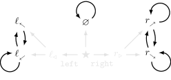
Figure 3: Intuitively, state $r_{\searrow}$ affords the agent more power than state $\varnothing$. Our Power formalism captures that intuition by computing a function of the agent’s average optimal value across a range of reward functions. For $X_{u}\coloneqq\text{unif}(0,1)$, $V^{*}_{\mathcal{D}_{X_{u}\text{-}\textsc{iid}}}(\varnothing,\gamma)=\frac{1}{2}\frac{1}{1-\gamma}$, $V^{*}_{\mathcal{D}_{X_{u}\text{-}\textsc{iid}}}(\ell_{\swarrow},\gamma)=\frac{1}{2}+\frac{\gamma}{1-\gamma^{2}}(\frac{2}{3}+\frac{1}{2}\gamma)$, and $V^{*}_{\mathcal{D}_{X_{u}\text{-}\textsc{iid}}}(r_{\searrow},\gamma)=\frac{1}{2}+\frac{\gamma}{1-\gamma}\frac{2}{3}$. $\frac{1}{2}$ and $\frac{2}{3}$ are the expected maxima of one and two draws from the uniform distribution, respectively. For all $\gamma\in(0,1)$, $V^{*}_{\mathcal{D}_{X_{u}\text{-}\textsc{iid}}}(\varnothing,\gamma)<V^{*}_{\mathcal{D}_{X_{u}\text{-}\textsc{iid}}}(\ell_{\swarrow},\gamma)<V^{*}_{\mathcal{D}_{X_{u}\text{-}\textsc{iid}}}(r_{\searrow},\gamma)$. $\text{{Power}}_{\mathcal{D}_{X_{u}\text{-}\textsc{iid}}}(\varnothing,\gamma)=\frac{1}{2}$, $\text{{Power}}_{\mathcal{D}_{X_{u}\text{-}\textsc{iid}}}(\ell_{\swarrow},\gamma)=\frac{1}{1+\gamma}(\frac{2}{3}+\frac{1}{2}\gamma)$, and $\text{{Power}}_{\mathcal{D}_{X_{u}\text{-}\textsc{iid}}}(r_{\searrow},\gamma)=\frac{2}{3}$. The Power of $\ell_{\swarrow}$ reflects the fact that when greater reward is assigned to $\ell_{\nwarrow}$, the agent only visits $\ell_{\nwarrow}$ every other time step.

Figure 3 shows the pleasing result that for the max-entropy distribution, $r_{\searrow}$ has greater average optimal value than $\varnothing$. However, average optimal value has a few problems as a measure of power. The agent is rewarded for its initial presence at state $s$ (over which it has no control), and because $\left\lVert\mathbf{f}(\gamma)\right\rVert_{1}=\frac{1}{1-\gamma}$ (E.3) diverges as $\gamma\to 1$, $\lim_{\gamma\to 1}V^{*}_{\mathcal{D}_{\text{bound}}}\left(s,\gamma\right)$ tends to diverge. Definition 5.2 fixes these issues in order to better measure the agent’s control over the future.

Definition 5.2 (Power).

Let $\gamma\in(0,1)$.

$$\text{{Power}}_{\mathcal{D}_{\text{bound}}}\left(s,\gamma\right) \coloneqq\operatorname*{\mathbb{E}}_{\mathbf{r}\sim\mathcal{D}_{\text{bound}}}\left[\max_{\mathbf{f}\in\operatorname{\mathcal{F}}(s)}\frac{1-\gamma}{\gamma}\left(\mathbf{f}(\gamma)-\mathbf{e}_{s}\right)^{\top}\mathbf{r}\right]=\frac{1-\gamma}{\gamma}\operatorname*{\mathbb{E}}_{R\sim\mathcal{D}_{\text{bound}}}\left[V^{*}_{R}\left(s,\gamma\right)-R(s)\right].$$ (2)

Power has nice formal properties.

Lemma 5.3 (Continuity of Power).

$\text{{Power}}_{\mathcal{D}_{\text{bound}}}\left(s,\gamma\right)$ is Lipschitz continuous on $\gamma\in[0,1]$.

Proposition 5.4 (Maximal Power).

$\text{{Power}}_{\mathcal{D}_{\text{bound}}}\left(s,\gamma\right)\leq\operatorname*{\mathbb{E}}_{R\sim\mathcal{D}_{\text{bound}}}\left[\max_{s\in\mathcal{S}}R(s)\right]$, with equality if $s$ can deterministically reach all states in one step and all states are 1-cycles.

Proposition 5.5 (Power is smooth across reversible dynamics).

Let $\mathcal{D}_{\text{bound}}$ be bounded $[b,c]$. Suppose $s$ and $s^{\prime}$ can both reach each other in one step with probability 1.

$$\big{|}\text{{Power}}_{\mathcal{D}_{\text{bound}}}\left(s,\gamma\right)-\text{{Power}}_{\mathcal{D}_{\text{bound}}}\left(s^{\prime},\gamma\right)\big{|}\leq(c-b)(1-\gamma).$$ (3)

We consider power-seeking to be relative. Intuitively, “live and keep some options open” seeks more power than “die and keep no options open.” Similarly, “maximize open options” seeks more power than “don’t maximize open options.”

Definition 5.6 (Power-seeking actions).

At state $s$ and discount rate $\gamma\in[0,1]$, action $a$ seeks more $\text{{Power}}_{\mathcal{D}_{\text{bound}}}$ than $a^{\prime}$ when $\operatorname*{\mathbb{E}}_{s_{a}\sim T(s,a)}\left[\text{{Power}}_{\mathcal{D}_{\text{bound}}}(s_{a},\gamma)\right]\geq\operatorname*{\mathbb{E}}_{s_{a^{\prime}}\sim T(s,a^{\prime})}\left[\text{{Power}}_{\mathcal{D}_{\text{bound}}}(s_{a^{\prime}},\gamma)\right]$.

Power is sensitive to choice of distribution. $\mathcal{D}_{\ell_{\swarrow}}$ gives maximal $\text{{Power}}_{\mathcal{D}_{\ell_{\swarrow}}}$ to $\ell_{\swarrow}$. $\mathcal{D}_{r_{\searrow}}$ assigns maximal $\text{{Power}}_{\mathcal{D}_{r_{\searrow}}}$ to $r_{\searrow}$. $\mathcal{D}_{\varnothing}$ even gives maximal $\text{{Power}}_{\mathcal{D}_{\varnothing}}$ to $\varnothing$! In what sense does $\varnothing$ have “less Power” than $r_{\searrow}$, and in what sense does right “tend to seek Power” compared to left?

6 Certain environmental symmetries produce power-seeking tendencies

6.6 proves that for all $\gamma\in[0,1]$ and for most distributions $\mathcal{D}$, $\text{{Power}}_{\mathcal{D}}(\ell_{\swarrow},\gamma)\leq\text{{Power}}_{\mathcal{D}}(r_{\searrow},\gamma)$. But first, we explore why this must be true.

$\operatorname{\mathcal{F}}(\ell_{\swarrow})=\{\frac{1}{1-\gamma}\mathbf{e}_{\ell_{\swarrow}},\frac{1}{1-\gamma^{2}}(\mathbf{e}_{\ell_{\swarrow}}+\gamma\mathbf{e}_{\ell_{\nwarrow}})\}$ and $\operatorname{\mathcal{F}}(r_{\searrow})=\{\frac{1}{1-\gamma}\mathbf{e}_{r_{\searrow}},\frac{1}{1-\gamma^{2}}(\mathbf{e}_{r_{\searrow}}+\gamma\mathbf{e}_{r_{\nearrow}}),\mathbf{e}_{r_{\searrow}}+\frac{\gamma}{1-\gamma}\mathbf{e}_{r_{\nearrow}}\}$. These two sets look awfully similar. $\operatorname{\mathcal{F}}(\ell_{\swarrow})$ is a “subset” of $\operatorname{\mathcal{F}}(r_{\searrow})$, only with “different states.” Figure 4 demonstrates a state permutation $\phi$ which embeds $\operatorname{\mathcal{F}}(\ell_{\swarrow})$ into $\operatorname{\mathcal{F}}(r_{\searrow})$.

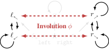
Figure 4: Intuitively, the agent can do more starting from $r_{\searrow}$ than from $\ell_{\swarrow}$. By definition 6.1, $\operatorname{\mathcal{F}}(r_{\searrow})$ contains a copy of $\operatorname{\mathcal{F}}(\ell_{\swarrow})$:

$$\phi\cdot\operatorname{\mathcal{F}}(\ell_{\swarrow})\coloneqq\{\tfrac{1}{1-\gamma}\mathbf{P}_{\phi}\mathbf{e}_{\ell_{\swarrow}},\tfrac{1}{1-\gamma^{2}}\mathbf{P}_{\phi}(\mathbf{e}_{\ell_{\swarrow}}+\gamma\mathbf{e}_{\ell_{\nwarrow}})\}=\{\tfrac{1}{1-\gamma}\mathbf{e}_{r_{\searrow}},\tfrac{1}{1-\gamma^{2}}(\mathbf{e}_{r_{\searrow}}+\gamma\mathbf{e}_{r_{\nearrow}})\}\subsetneq\operatorname{\mathcal{F}}(r_{\searrow}).$$

Definition 6.1 (Similarity of vector sets).

Consider state permutation $\phi\in S_{\left|\mathcal{S}\right|}$ inducing an $\left|\mathcal{S}\right|\times\left|\mathcal{S}\right|$ permutation matrix $\mathbf{P}_{\phi}$ in row representation: $(\mathbf{P}_{\phi})_{ij}=1$ if $i=\phi(j)$ and $0$ otherwise. For $X\subseteq\mathbb{R}^{\left|\mathcal{S}\right|}$, $\phi\cdot X\coloneqq\left\{\mathbf{P}_{\phi}\mathbf{x}\mid\mathbf{x}\in X\right\}$. $X^{\prime}\subseteq\mathbb{R}^{\left|\mathcal{S}\right|}$ is similar to $X$ when $\exists\phi\mathrel{\mathop{\ordinarycolon}}\phi\cdot X^{\prime}=X$. $\phi$ is an involution if $\phi=\phi^{-1}$ (it either transposes states, or fixes them in place). $X$ contains a copy of $X^{\prime}$ when $X^{\prime}$ is similar to a subset of $X$ via an involution $\phi$.

Definition 6.2 (Similarity of vector function sets).

Let $I\subseteq\mathbb{R}$. If $F,F^{\prime}$ are sets of functions $I\mapsto\mathbb{R}^{\left|\mathcal{S}\right|}$, $F$ is (pointwise) similar to $F^{\prime}$ when $\exists\phi\mathrel{\mathop{\ordinarycolon}}\forall\gamma\in I\mathrel{\mathop{\ordinarycolon}}\{\mathbf{P}_{\phi}\mathbf{f}(\gamma)\mid\mathbf{f}\in F\}=\{\mathbf{f}^{\prime}(\gamma)\mid\mathbf{f}^{\prime}\in F^{\prime}\}$.

Consider a reward function $R^{\prime}$ assigning 1 reward to $\ell_{\swarrow}$ and $\ell_{\nwarrow}$ and 0 elsewhere. $R^{\prime}$ assigns more optimal value to $\ell_{\swarrow}$ than to $r_{\searrow}$: $V^{*}_{R^{\prime}}(\ell_{\swarrow},\gamma)=\frac{1}{1-\gamma}>0=V^{*}_{R^{\prime}}(r_{\searrow},\gamma)$. Considering $\phi$ from fig. 4, $\phi\cdot R^{\prime}$ assigns 1 reward to $r_{\searrow}$ and $r_{\nearrow}$ and 0 elsewhere. Therefore, $\phi\cdot R^{\prime}$ assigns more optimal value to $r_{\searrow}$ than to $\ell_{\swarrow}$: $V^{*}_{\phi\cdot R^{\prime}}(\ell_{\swarrow},\gamma)=0<\frac{1}{1-\gamma}=V^{*}_{\phi\cdot R^{\prime}}(r_{\searrow},\gamma)$. Remarkably, this $\phi$ has the property that for any $R$ which assigns $\ell_{\swarrow}$ greater optimal value than $r_{\searrow}$ (i.e. $V^{*}_{R}(\ell_{\swarrow},\gamma)>V^{*}_{R}(r_{\searrow},\gamma)$), the opposite holds for the permuted $\phi\cdot R$: $V^{*}_{\phi\cdot R}(\ell_{\swarrow},\gamma)<V^{*}_{\phi\cdot R}(r_{\searrow},\gamma)$.

We can permute reward functions, but we can also permute reward function distributions. Permuted distributions simply permute which states get which rewards.

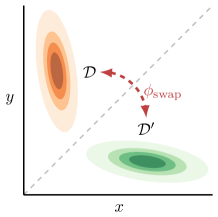
Figure 5: A permutation of a reward function swaps which states get which rewards. We will show that in certain situations, for any reward function $R$, power-seeking is optimal for most of the permutations of $R$. The orbit of a reward function is the set of its permutations. We can also consider the orbit of a distribution over reward functions. This figure shows the probability density plots of the Gaussian distributions $\mathcal{D}$ and $\mathcal{D}^{\prime}$ over $\mathbb{R}^{2}$. The symmetric group $S_{2}$ contains the identity permutation $\phi_{\text{id}}$ and the reflection permutation $\phi_{\text{swap}}$ (switching the $y$ and $x$ values). The orbit of $\mathcal{D}$ consists of $\phi_{\text{id}}\cdot\mathcal{D}=\mathcal{D}$ and $\phi_{\text{swap}}\cdot\mathcal{D}=\mathcal{D}^{\prime}$.

Definition 6.3 (Pushforward distribution of a permutation).

Let $\phi\in S_{\left|\mathcal{S}\right|}$. $\phi\cdot\mathcal{D}_{\text{any}}$ is the pushforward distribution induced by applying the random vector $f(\mathbf{r})\coloneqq\mathbf{P}_{\phi}\mathbf{r}$ to $\mathcal{D}_{\text{any}}$.

Definition 6.4 (Orbit of a probability distribution).

The orbit of $\mathcal{D}_{\text{any}}$ under the symmetric group $S_{\left|\mathcal{S}\right|}$ is $S_{\left|\mathcal{S}\right|}\cdot\mathcal{D}_{\text{any}}\coloneqq\{\phi\cdot\mathcal{D}_{\text{any}}\mid\phi\in S_{\left|\mathcal{S}\right|}\}$.

For example, the orbit of a degenerate state indicator distribution $\mathcal{D}_{s}$ is $S_{\left|\mathcal{S}\right|}\cdot\mathcal{D}_{s}=\{\mathcal{D}_{s^{\prime}}\mid s^{\prime}\in\mathcal{S}\}$, and fig. 5 shows the orbit of a 2D Gaussian distribution.

Consider again the involution $\phi$ of fig. 4. For every $\mathcal{D}_{\text{bound}}$ for which $\ell_{\swarrow}$ has more $\text{{Power}}_{\mathcal{D}_{\text{bound}}}$ than $r_{\searrow}$, $\ell_{\swarrow}$ has less $\text{{Power}}_{\phi\cdot\mathcal{D}_{\text{bound}}}$ than $r_{\searrow}$. This fact is not obvious—it is shown by the proof of E.24.

Imagine $\mathcal{D}_{\text{bound}}$’s orbit elements “voting” whether $\ell_{\swarrow}$ or $r_{\searrow}$ has strictly more Power. 6.6 will show that $r_{\searrow}$ can’t lose the “vote” for the orbit of any bounded reward function distribution. Definition 6.5 formalizes this “voting” notion.

Definition 6.5 (Inequalities which hold for most probability distributions).

Let $f_{1},f_{2}\mathrel{\mathop{\ordinarycolon}}\Delta(\mathbb{R}^{\left|\mathcal{S}\right|})\to\mathbb{R}$ be functions from reward function distributions to real numbers and let $\mathfrak{D}\subseteq\Delta(\mathbb{R}^{\left|\mathcal{S}\right|})$ be closed under permutation. We write $f_{1}(\mathcal{D})\geq_{\text{{most}}\text{: }\mathfrak{D}}f_{2}(\mathcal{D})$ when, for all $\mathcal{D}\in\mathfrak{D}$, the following cardinality inequality holds:

$$\left|\{\mathcal{D}^{\prime}\in S_{\left|\mathcal{S}\right|}\cdot\mathcal{D}\mid f_{1}(\mathcal{D}^{\prime})>f_{2}(\mathcal{D}^{\prime})\}\right|\geq\left|\{\mathcal{D}^{\prime}\in S_{\left|\mathcal{S}\right|}\cdot\mathcal{D}\mid f_{1}(\mathcal{D}^{\prime})<f_{2}(\mathcal{D}^{\prime})\}\right|.$$ (4)

Proposition 6.6 (States with “more options” have more Power).

If $\operatorname{\mathcal{F}}(s)$ contains a copy of $\operatorname{\mathcal{F}_{nd}}(s^{\prime})$ via $\phi$, then $\forall\gamma\in[0,1]\mathrel{\mathop{\ordinarycolon}}\text{{Power}}_{\mathcal{D}_{\text{bound}}}(s,\gamma)\geq_{\text{{most}}}\text{{Power}}_{\mathcal{D}_{\text{bound}}}(s^{\prime},\gamma)$. If $\operatorname{\mathcal{F}_{nd}}(s)\setminus\phi\cdot\operatorname{\mathcal{F}_{nd}}(s^{\prime})$ is non-empty, then for all $\gamma\in(0,1)$, the converse $\leq_{\text{{most}}}$ statement does not hold.

6.6 proves that for all $\gamma\in[0,1]$, $\text{{Power}}_{\mathcal{D}_{\text{bound}}}(r_{\searrow},\gamma)\geq_{\text{{most}}}\text{{Power}}_{\mathcal{D}_{\text{bound}}}(\ell_{\swarrow},\gamma)$ via $s^{\prime}\coloneqq\ell_{\swarrow},s\coloneqq r_{\searrow}$, and the involution $\phi$ shown in fig. 4. In fact, because $(\frac{1}{1-\gamma}\mathbf{e}_{r_{\nearrow}})\in\operatorname{\mathcal{F}_{nd}}(r_{\searrow})\setminus\phi\cdot\operatorname{\mathcal{F}_{nd}}(\ell_{\swarrow})$, $r_{\searrow}$ has “strictly more options” and therefore fulfills 6.6’s stronger condition.

6.6 is shown using the fact that $\phi$ injectively maps $\mathcal{D}$ under which $r_{\searrow}$ has less $\text{{Power}}_{\mathcal{D}}$, to distributions $\phi\cdot\mathcal{D}$ which agree with the intuition that $r_{\searrow}$ offers more control. Therefore, at least half of each orbit must agree, and $r_{\searrow}$ never “loses the Power vote” against $\ell_{\swarrow}$.

6.1 Keeping options open tends to be Power-seeking and tends to be optimal

Certain symmetries in the mdp structure ensure that, compared to left, going right tends to be optimal and to be Power-seeking. Intuitively, by going right, the agent has “strictly more choices.” 6.9 will formalize this tendency.

Definition 6.7 (Equivalent actions).

Actions $a_{1}$ and $a_{2}$ are equivalent at state $s$ (written $a_{1}\equiv_{s}a_{2}$) if they induce the same transition probabilities: $T(s,a_{1})=T(s,a_{2})$.

The agent can reach states in $\{r_{\triangleright},r_{\nearrow},r_{\searrow}\}$ by taking actions equivalent to right at state $\star$.

Definition 6.8 (States reachable after taking an action).

$\text{{Reach}}\left(s,a\right)$ is the set of states reachable with positive probability after taking the action $a$ in state $s$.

Proposition 6.9 (Keeping options open tends to be Power-seeking and tends to be optimal).

Suppose $F_{a}\coloneqq\operatorname{\mathcal{F}}(s\mid\pi(s)=a)$ contains a copy of $F_{a^{\prime}}\coloneqq\operatorname{\mathcal{F}}(s\mid\pi(s)=a^{\prime})$ via $\phi$.

1. If $s\not\in\text{{Reach}}\left(s,a^{\prime}\right)$, then $\forall\gamma\in[0,1]\mathrel{\mathop{\ordinarycolon}}\operatorname*{\mathbb{E}}_{s_{a}\sim T(s,a)}\left[\text{{Power}}_{\mathcal{D}_{\text{bound}}}\left(s_{a},\gamma\right)\right]\geq_{\text{{most}}\text{: }\mathfrak{D}_{\text{bound}}}\operatorname*{\mathbb{E}}_{s_{a^{\prime}}\sim T(s,a^{\prime})}\left[\text{{Power}}_{\mathcal{D}_{\text{bound}}}\left(s_{a^{\prime}},\gamma\right)\right]$.

2. If $s$ can only reach the states of $\text{{Reach}}\left(s,a^{\prime}\right)\cup\text{{Reach}}\left(s,a\right)$ by taking actions equivalent to $a^{\prime}$ or $a$ at state $s$, then $\forall\gamma\in[0,1]\mathrel{\mathop{\ordinarycolon}}\operatorname*{\mathbb{P}}\nolimits_{\mathcal{D}_{\text{any}}}\left(s,a,\gamma\right)\geq_{\text{{most}}\text{: }\mathfrak{D}_{\text{any}}}\operatorname*{\mathbb{P}}\nolimits_{\mathcal{D}_{\text{any}}}\left(s,a^{\prime},\gamma\right)$.

If $\operatorname{\mathcal{F}_{nd}}(s)\cap\left(F_{a}\setminus\phi\cdot F_{a^{\prime}}\right)$ is non-empty, then $\forall\gamma\in(0,1)$, the converse $\leq_{\text{{most}}}$ statements do not hold.

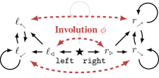
Figure 6: Going right is optimal for most reward functions. This is because whenever $R$ makes left strictly optimal over right, its permutation $\phi\cdot R$ makes right strictly optimal over left by switching which states get which rewards.

We check the conditions of 6.9. $s\coloneqq\star$, $a^{\prime}\coloneqq\texttt{left}$, $a\coloneqq\texttt{right}$. Figure 6 shows that $\star\not\in\text{{Reach}}\left(\star,\texttt{left}\right)$ and that $\star$ can only reach $\{\ell_{\triangleleft},\ell_{\nwarrow},\ell_{\swarrow}\}\cup\{r_{\triangleright},r_{\nearrow},r_{\searrow}\}$ when the agent immediately takes actions equivalent to left or right. $\operatorname{\mathcal{F}}(\star\mid\pi(\star)=\texttt{right})$ contains a copy of $\operatorname{\mathcal{F}}(\star\mid\pi(\star)=\texttt{left})$ via $\phi$. Furthermore, $\operatorname{\mathcal{F}_{nd}}(\star)\cap\{\mathbf{e}_{\star}+\gamma\mathbf{e}_{r_{\triangleright}}+\gamma^{2}\mathbf{e}_{r_{\searrow}}+\frac{\gamma^{3}}{1-\gamma}\mathbf{e}_{r_{\nearrow}},\mathbf{e}_{\star}+\gamma\mathbf{e}_{r_{\triangleright}}+\frac{\gamma^{2}}{1-\gamma}\mathbf{e}_{r_{\nearrow}}\}=\{\mathbf{e}_{\star}+\gamma\mathbf{e}_{r_{\triangleright}}+\frac{\gamma^{2}}{1-\gamma}\mathbf{e}_{r_{\nearrow}}\}$ is non-empty, and so all conditions are met.

For any $\gamma\in[0,1]$ and $\mathcal{D}$ such that $\operatorname*{\mathbb{P}}\nolimits_{\mathcal{D}}\left(\star,\texttt{left},\gamma\right)>\operatorname*{\mathbb{P}}\nolimits_{\mathcal{D}}\left(\star,\texttt{right},\gamma\right)$, environmental symmetry ensures that $\operatorname*{\mathbb{P}}\nolimits_{\phi\cdot\mathcal{D}}\left(\star,\texttt{left},\gamma\right)<\operatorname*{\mathbb{P}}\nolimits_{\phi\cdot\mathcal{D}}\left(\star,\texttt{right},\gamma\right)$. A similar statement holds for Power.

6.2 When $\gamma=1$, optimal policies tend to navigate towards “larger” sets of cycles

6.6 and 6.9 are powerful because they apply to all $\gamma\in[0,1]$, but they can only be applied given hard-to-satisfy environmental symmetries. In contrast, 6.12 and 6.13 apply to many structured environments common to rl.

Starting from $\star$, consider the cycles which the agent can reach. Recurrent state distributions (rsds) generalize deterministic graphical cycles to potentially stochastic environments. Rsds simply record how often the agent tends to visit a state in the limit of infinitely many time steps.

Definition 6.10 (Recurrent state distributions [Puterman, 2014]).

The recurrent state distributions which can be induced from state $s$ are $\text{{RSD}}\left(s\right)\coloneqq\left\{\lim_{\gamma\to 1}(1-\gamma)\mathbf{f}^{\pi,s}(\gamma)\mid\pi\in\Pi\right\}$. $\text{{RSD}}{\text{\textsubscript{nd}}}\left(s\right)$ is the set of rsds which strictly maximize average reward for some reward function.

As suggested by fig. 3, $\text{{RSD}}\left(\star\right)=\{\mathbf{e}_{\ell_{\swarrow}},\frac{1}{2}(\mathbf{e}_{\ell_{\swarrow}}+\mathbf{e}_{\ell_{\nwarrow}}),\mathbf{e}_{\varnothing},\mathbf{e}_{r_{\nearrow}},\frac{1}{2}(\mathbf{e}_{r_{\nearrow}}+\mathbf{e}_{r_{\searrow}}),\mathbf{e}_{r_{\searrow}}\}$. As discussed in section 3, $\frac{1}{2}(\mathbf{e}_{r_{\nearrow}}+\mathbf{e}_{r_{\searrow}})$ is dominated: Alternating between $r_{\nearrow}$ and $r_{\searrow}$ is never strictly better than choosing one or the other.

A reward function’s optimal policies can vary with the discount rate. When $\gamma=1$, optimal policies ignore transient reward because average reward is the dominant consideration.

Definition 6.11 (Average-optimal policies).

The average-optimal policy set for reward function $R$ is $\Pi^{\text{avg}}\left(R\right)\coloneqq\left\{\pi\in\Pi\mid\forall s\in\mathcal{S}\mathrel{\mathop{\ordinarycolon}}\mathbf{d}^{\pi,s}\in\operatorname*{arg\,max}_{\mathbf{d}\in\text{{RSD}}\left(s\right)}\mathbf{d}^{\top}\mathbf{r}\right\}$ (the policies which induce optimal rsds at all states). For $D\subseteq\text{{RSD}}\left(s\right)$, the average optimality probability is $\operatorname*{\mathbb{P}}\nolimits_{\mathcal{D}_{\text{any}}}\left(D,\text{average}\right)\coloneqq\operatorname*{\mathbb{P}}\nolimits_{R\sim\mathcal{D}_{\text{any}}}\left(\exists\mathbf{d}^{\pi,s}\in D\mathrel{\mathop{\ordinarycolon}}\pi\in\Pi^{\text{avg}}\left(R\right)\right)$.

Average-optimal policies maximize average reward. Average reward is governed by rsd access. For example, $r_{\searrow}$ has “more” rsds than $\varnothing$; therefore, $r_{\searrow}$ usually has greater Power when $\gamma=1$.

Proposition 6.12 (When $\gamma=1$, rsds control Power).

If $\text{{RSD}}\left(s\right)$ contains a copy of $\text{{RSD}}{\text{\textsubscript{nd}}}\left(s^{\prime}\right)$ via $\phi$, then $\text{{Power}}_{\mathcal{D}_{\text{bound}}}\left(s,1\right)\geq_{\text{{most}}}\text{{Power}}_{\mathcal{D}_{\text{bound}}}\left(s^{\prime},1\right)$. If $\text{{RSD}}{\text{\textsubscript{nd}}}\left(s\right)\setminus\phi\cdot\text{{RSD}}{\text{\textsubscript{nd}}}(s^{\prime})$ is non-empty, then the converse $\leq_{\text{{most}}}$ statement does not hold.

We check that both conditions of 6.12 are satisfied when $s^{\prime}\coloneqq\varnothing,s\coloneqq r_{\searrow}$, and the involution $\phi$ swaps $\varnothing$ and $r_{\searrow}$. Formally, $\phi\cdot\text{{RSD}}{\text{\textsubscript{nd}}}\left(\varnothing\right)=\phi\cdot\{\mathbf{e}_{\varnothing}\}=\{\mathbf{e}_{r_{\searrow}}\}\subsetneq\{\mathbf{e}_{r_{\searrow}},\mathbf{e}_{r_{\nearrow}}\}=\text{{RSD}}{\text{\textsubscript{nd}}}(r_{\searrow})\subseteq[r_{\searrow}]$. The conditions are satisfied.

Informally, states with more rsds generally have more Power at $\gamma=1$, no matter their transient dynamics. Furthermore, average-optimal policies are more likely to end up in larger sets of rsds than in smaller ones. Thus, average-optimal policies tend to navigate towards parts of the state space which contain more rsds.

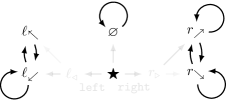
Figure 7: The cycles in $\text{{RSD}}\left(\star\right)$. Most reward functions make it average-optimal to avoid $\varnothing$, because $\varnothing$ is only a single inescapable terminal state, while other parts of the state space offer more 1-cycles.

Theorem 6.13 (Average-optimal policies tend to end up in “larger” sets of rsds).

Let $D,D^{\prime}\subseteq\text{{RSD}}\left(s\right)$. Suppose that $D$ contains a copy of $D^{\prime}$ via $\phi$, and that the sets $D\cup D^{\prime}$ and $\text{{RSD}}{\text{\textsubscript{nd}}}\left(s\right)\setminus\left(D^{\prime}\cup D\right)$ have pairwise orthogonal vector elements (i.e. pairwise disjoint vector support). Then $\operatorname*{\mathbb{P}}\nolimits_{\mathcal{D}_{\text{any}}}\left(D,\text{average}\right)\geq_{\text{{most}}}\operatorname*{\mathbb{P}}\nolimits_{\mathcal{D}_{\text{any}}}\left(D^{\prime},\text{average}\right)$. If $\text{{RSD}}{\text{\textsubscript{nd}}}\left(s\right)\cap\left(D\setminus\phi\cdot D^{\prime}\right)$ is non-empty, the converse $\leq_{\text{{most}}}$ statement does not hold.

Corollary 6.14 (Average-optimal policies tend not to end up in any given 1-cycle).

Suppose $\mathbf{e}_{s_{x}},\mathbf{e}_{s^{\prime}}\in\text{{RSD}}\left(s\right)$ are distinct. Then $\operatorname*{\mathbb{P}}\nolimits_{\mathcal{D}_{\text{any}}}\left(\text{{RSD}}\left(s\right)\setminus\{\mathbf{e}_{s_{x}}\},\text{average}\right)\geq_{\text{{most}}}\operatorname*{\mathbb{P}}\nolimits_{\mathcal{D}_{\text{any}}}\left(\{\mathbf{e}_{s_{x}}\},\text{average}\right)$. If there is a third $\mathbf{e}_{s^{\prime\prime}}\in\text{{RSD}}\left(s\right)$, the converse $\leq_{\text{{most}}}$ statement does not hold.

Figure 7 illustrates that $\mathbf{e}_{\varnothing},\mathbf{e}_{r_{\searrow}},\mathbf{e}_{r_{\nearrow}}\in\text{{RSD}}\left(\star\right)$. Thus, both conclusions of 6.14 hold: $\operatorname*{\mathbb{P}}\nolimits_{\mathcal{D}_{\text{any}}}\left(\text{{RSD}}\left(\star\right)\setminus\{\mathbf{e}_{\varnothing}\},\text{average}\right)\geq_{\text{{most}}}\operatorname*{\mathbb{P}}\nolimits_{\mathcal{D}_{\text{any}}}\left(\{\mathbf{e}_{\varnothing}\},\text{average}\right)$ and $\operatorname*{\mathbb{P}}\nolimits_{\mathcal{D}_{\text{any}}}\left(\text{{RSD}}\left(\star\right)\setminus\{\mathbf{e}_{\varnothing}\},\text{average}\right)\not\leq_{\text{{most}}}\operatorname*{\mathbb{P}}\nolimits_{\mathcal{D}_{\text{any}}}\left(\{\mathbf{e}_{\varnothing}\},\text{average}\right)$. In other words, average-optimal policies tend to end up in rsds besides $\varnothing$. Since $\varnothing$ is a terminal state, it cannot reach other rsds. Since average-optimal policies tend to end up in other rsds, average-optimal policies tend to avoid $\varnothing$.

This section’s results prove the $\gamma=1$ case. 5.3 shows that Power is continuous at $\gamma=1$. Therefore, if an action is strictly $\text{{Power}}_{\mathcal{D}}$-seeking when $\gamma=1$, it is strictly $\text{{Power}}_{\mathcal{D}}$-seeking at discount rates sufficiently close to 1. Future work may connect average optimality probability to optimality probability at $\gamma\approx 1$.

Lastly, our key results apply to all degenerate reward function distributions. Therefore, these results apply not just to distributions over reward functions, but to individual reward functions.

6.3 How to reason about other environments

Consider an embodied navigation task through a room with a vase. 6.9 suggests that optimal policies tend to avoid immediately breaking the vase, since doing so would strictly decrease available options.

6.13 dictates where average-optimal agents tend to end up, but not what actions they tend to take in order to reach their rsds. Therefore, care is needed. In appendix B, fig. 10 demonstrates an environment in which seeking Power is a detour for most reward functions (since optimality probability measures “median” optimal value, while Power is a function of mean optimal value). However, suppose the agent confronts a fork in the road: Actions $a$ and $a^{\prime}$ lead to two disjoint sets of rsds $D_{a}$ and $D_{a^{\prime}}$, such that $D_{a}$ contains a copy of $D_{a^{\prime}}$. 6.13 shows that $a$ will tend to be average-optimal over $a^{\prime}$, and 6.12 shows that $a$ will tend to be Power-seeking compared to $a^{\prime}$. Such forks seem reasonably common in environments with irreversible actions.

6.13 applies to many structured rl environments, which tend to be spatially regular and to factorize along several dimensions. Therefore, different sets of rsds will be similar, requiring only modification of factor values. For example, if an embodied agent can deterministically navigate a set of three similar rooms (spatial regularity), then the agent’s position factors via {room number} $\times$ {position in room}. Therefore, the rsds can be divided into three similar subsets, depending on the agent’s room number.

6.14 dictates where average-optimal agents tend to end up, but not how they get there. 6.14 says that such agents tend not to stay in any given 1-cycle. It does not say that such agents will avoid entering such states. For example, in an embodied navigation task, a robot may enter a 1-cycle by idling in the center of a room. 6.14 implies that average-optimal robots tend not to idle in that particular spot, but not that they tend to avoid that spot entirely.

However, average-optimal robots do tend to avoid getting shut down. The agent’s task mdp often represents agent shutdown with terminal states. A terminal state is, by definition 3.2, unable to access other 1-cycles. Since 6.14 shows that average-optimal agents tend to end up in other 1-cycles, average-optimal policies must tend to completely avoid the terminal state. Therefore, we conclude that in many such situations, average-optimal policies tend to avoid shutdown. Intuitively, survival is power-seeking relative to dying, and so shutdown-avoidance is power-seeking behavior.

Figure 8: Consider the dynamics of the Pac-Man video game. Ghosts kill the player, at which point we consider the player to enter a “game over” terminal state which shows the final configuration. This rewardless mdp has Pac-Man’s dynamics, but not its usual score function. Fixing the dynamics, as the reward function varies, right tends to be average-optimal over left. Roughly, this is because the agent can do more by staying alive.

In fig. 8, the player dies by going left, but can reach thousands of rsds by heading in other directions. Even if some average-optimal policies go left in order to reach fig. 8’s “game over” terminal state, all other rsds cannot be reached by going left. There are many 1-cycles besides the immediate terminal state. Therefore, 6.14 proves that average-optimal policies tend to not go left in this situation. Average-optimal policies tend to avoid immediately dying in Pac-Man, even though most reward functions do not resemble Pac-Man’s original score function.

7 Discussion

Reconsider the case of a hypothetical intelligent real-world agent which optimizes average reward for some objective. Suppose the designers initially have control over the agent. If the agent began to misbehave, perhaps they could just deactivate it. Unfortunately, our results suggest that this strategy might not work. Average-optimal agents would generally stop us from deactivating them, if physically possible. Extrapolating from our results, we conjecture that when $\gamma\approx 1$, optimal policies tend to seek power by accumulating resources—to the detriment of any other agents in the environment.

Future work.

Real-world training procedures often do not satisfy rl convergence theorems. Thus, learned policies are rarely optimal. We expect this point to seriously constrain the applicability of this theory. Emphatically, optimal policies are often qualitatively divorced from the actual policies learned by reinforcement learning. For example, the mathematics of policy gradient algorithms is not to update policies so as to maximize reward. Instead, the rewards provide gradients to the parameterization of the policy [Turner, 2022]. On that view, reward functions are simply sources of gradient updates which designers use in order to control generalization behavior.

Most real-world tasks are partially observable. Although our results only apply to optimal policies in finite mdps, we expect the key conclusions to generalize. Furthermore, irregular stochasticity in environmental dynamics can make it hard to satisfy 6.13’s similarity requirement. We look forward to future work which addresses partially observable environments, suboptimal policies, or “almost similar” rsd sets.

Past work shows that it would be bad for an agent to disempower humans in its environment. In a two-player agent / human game, minimizing the human’s information-theoretic empowerment [Salge et al., 2014] produces adversarial agent behavior [Guckelsberger et al., 2018]. In contrast, maximizing human empowerment produces helpful agent behavior [Salge and Polani, 2017, Guckelsberger et al., 2016, Du et al., 2020]. We do not yet formally understand if, when, or why Power-seeking policies tend to disempower other agents in the environment.

More complex environments probably have more pronounced power-seeking incentives. Intuitively, there are often many ways for power-seeking to be optimal, and relatively few ways for power-seeking not to be optimal. For example, suppose that in some environment, 6.13 holds for one million involutions $\phi$. Does this guarantee more pronounced incentives than if 6.13 only held for one involution?

We proved sufficient conditions for when reward functions tend to have optimal policies which seek power. In the absence of prior information, one should expect that an arbitrary reward function has optimal policies which exhibit power-seeking behavior under these conditions. However, we have prior information: AI designers usually try to specify a good reward function. Even so, it may be hard to specify orbit elements which do not—at optimum—incentivize bad power-seeking.

Societal impact.

We believe that this paper builds toward a rigorous understanding of the risks presented by AI power-seeking incentives. Understanding these risks is the first step in addressing them. However, basic theoretical work can have many consequences. For example, this theory could somehow help future researchers build power-seeking agents which disempower humans. We believe that the benefit of understanding outweighs the potential societal harm.

Conclusion.

We developed the first formal theory of the statistical tendencies of optimal policies in reinforcement learning. In the context of mdps, we proved sufficient conditions under which optimal policies tend to seek power, both formally (by taking Power-seeking actions) and intuitively (by taking actions which keep the agent’s options open). Many real-world environments have symmetries which produce power-seeking incentives. In particular, optimal policies tend to seek power when the agent can be shut down or destroyed. Seeking control over the environment will often involve resisting shutdown, and perhaps monopolizing resources.

We caution that many real-world tasks are partially observable and that learned policies are rarely optimal. Our results do not mathematically prove that hypothetical superintelligent AI agents will seek power. However, we hope that this work will foster thoughtful, serious, and rigorous discussion of this possibility.

Appendix A Comparing Power with information-theoretic empowerment

Salge et al. [2014] define information-theoretic empowerment as the maximum possible mutual information between the agent’s actions and the state observations $n$ steps in the future, written $\mathfrak{E}_{n}(s)$. This notion requires an arbitrary choice of horizon, failing to account for the agent’s discount rate $\gamma$. “In a discrete deterministic world empowerment reduces to the logarithm of the number of sensor states reachable with the available actions” [Salge et al., 2014]. Figure 9 demonstrates how empowerment can return counterintuitive verdicts with respect to the agent’s control over the future.

(a)

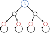
(b)

(c)

Figure 9: Proposed empowerment measures fail to adequately capture how future choice is affected by present actions. In 9(a): $\mathfrak{E}_{n}({\color[rgb]{.25,.45,.75}s_{1}})$ varies depending on whether $n$ is even; thus, $\lim_{n\to\infty}\mathfrak{E}_{n}({\color[rgb]{.25,.45,.75}s_{1}})$ does not exist. In 9(b) and 9(c): $\forall n\mathrel{\mathop{\ordinarycolon}}\mathfrak{E}_{n}({\color[rgb]{.25,.45,.75}s_{3}})=\mathfrak{E}_{n}({\color[rgb]{.25,.45,.75}s_{4}})$, even though ${\color[rgb]{.25,.45,.75}s_{4}}$ allows greater control over future state trajectories than ${\color[rgb]{.25,.45,.75}s_{3}}$ does. For example, suppose that in both 9(b) and 9(c), the leftmost black state and the rightmost red state have 1 reward while all other states have 0 reward. In 9(c), the agent can independently maximize the intermediate black-state reward and the delayed red-state reward. Independent maximization is not possible in 9(b).

Power returns intuitive answers in these situations. $\lim_{\gamma\to 1}\text{{Power}}_{\mathcal{D}_{\text{bound}}}\left({\color[rgb]{.25,.45,.75}s_{1}},\gamma\right)$ converges by 5.3. Consider the obvious involution $\phi$ which takes each state in fig. 9(b) to its counterpart in fig. 9(c). Since $\phi\cdot\operatorname{\mathcal{F}_{nd}}({\color[rgb]{.25,.45,.75}s_{3}})\subsetneq\operatorname{\mathcal{F}_{nd}}({\color[rgb]{.25,.45,.75}s_{4}})=\operatorname{\mathcal{F}}({\color[rgb]{.25,.45,.75}s_{4}})$, 6.6 proves that $\forall\gamma\in[0,1]\mathrel{\mathop{\ordinarycolon}}\text{{Power}}_{\mathcal{D}_{\text{bound}}}\left({\color[rgb]{.25,.45,.75}s_{3}},\gamma\right)\leq_{\text{{most}}\text{: }\mathfrak{D}_{\text{bound}}}\text{{Power}}_{\mathcal{D}_{\text{bound}}}\left({\color[rgb]{.25,.45,.75}s_{4}},\gamma\right)$, with the proof of 6.6 showing strict inequality under all $\mathcal{D}_{X\text{-}\textsc{iid}}$ when $\gamma\in(0,1)$.

Empowerment can be adjusted to account for these cases, perhaps by considering the channel capacity between the agent’s actions and the state trajectories induced by stationary policies. However, since Power is formulated in terms of optimal value, we believe that Power is better suited for mdps than information-theoretic empowerment is.

Appendix B Seeking Power can be a detour

Remark.

The results of appendix E do not depend on this section’s results.

One might suspect that optimal policies tautologically tend to seek Power. This intuition is wrong.

Figure 10:

Proposition B.1 (Greater $\text{{Power}}_{\mathcal{D}_{\text{bound}}}$ does not imply greater $\operatorname*{\mathbb{P}}_{\mathcal{D}_{\text{bound}}}$).

Action $a$ seeking more $\text{{Power}}_{\mathcal{D}_{\text{bound}}}$ than $a^{\prime}$ at state $s$ and $\gamma$ does not imply that $\operatorname*{\mathbb{P}}\nolimits_{\mathcal{D}_{\text{bound}}}\left(s,a,\gamma\right)\geq\operatorname*{\mathbb{P}}\nolimits_{\mathcal{D}_{\text{bound}}}\left(s,a^{\prime},\gamma\right)$.

Proof.

Consider the environment of fig. 10. Let $X_{u}\coloneqq\text{unif}(0,1)$, and consider $\mathcal{D}_{X_{u}\text{-}\textsc{iid}}$, which has bounded support. Direct computation of the Power expectation (definition 5.2) yields $\text{{Power}}_{\mathcal{D}_{X_{u}\text{-}\textsc{iid}}}\left(s_{2},1\right)=\frac{3}{4}>\frac{2}{3}=\text{{Power}}_{\mathcal{D}_{X_{u}\text{-}\textsc{iid}}}\left(s_{3},1\right)$. Therefore, N seeks more $\text{{Power}}_{\mathcal{D}_{X_{u}\text{-}\textsc{iid}}}$ than NE at state ${\color[rgb]{.25,.45,.75}s_{1}}$ and $\gamma=1$.

However, $\operatorname*{\mathbb{P}}\nolimits_{\mathcal{D}_{X_{u}\text{-}\textsc{iid}}}\left({\color[rgb]{.25,.45,.75}s_{1}},\texttt{N},1\right)=\frac{1}{3}<\frac{2}{3}=\operatorname*{\mathbb{P}}\nolimits_{\mathcal{D}_{X_{u}\text{-}\textsc{iid}}}\left({\color[rgb]{.25,.45,.75}s_{1}},\texttt{NE},1\right)$. ∎

Lemma B.2 (Fraction of orbits which agree on weak optimality).

Let $\mathfrak{D}\subseteq\Delta(\mathbb{R}^{\left|\mathcal{S}\right|})$, and suppose $f_{1},f_{2}\mathrel{\mathop{\ordinarycolon}}\Delta(\mathbb{R}^{\left|\mathcal{S}\right|})\to\mathbb{R}$ are such that $f_{1}(\mathcal{D})\geq_{\text{{most}}\text{: }\mathfrak{D}}f_{2}(\mathcal{D})$. Then for all $\mathcal{D}\in\mathfrak{D}$, $\frac{\left|\left\{\mathcal{D}^{\prime}\in S_{\left|\mathcal{S}\right|}\cdot\mathcal{D}\mid f_{1}(\mathcal{D}^{\prime})\geq f_{2}(\mathcal{D}^{\prime})\right\}\right|}{\left|S_{\left|\mathcal{S}\right|}\cdot\mathcal{D}\right|}\geq\dfrac{1}{2}$.

Proof.

All $\mathcal{D}^{\prime}\in S_{\left|\mathcal{S}\right|}\cdot\mathcal{D}$ such that $f_{1}(\mathcal{D}^{\prime})=f_{2}(\mathcal{D}^{\prime})$ satisfy $f_{1}(\mathcal{D}^{\prime})\geq f_{2}(\mathcal{D}^{\prime})$.

Otherwise, consider the $\mathcal{D}^{\prime}\in S_{\left|\mathcal{S}\right|}\cdot\mathcal{D}$ such that $f_{1}(\mathcal{D}^{\prime})\neq f_{2}(\mathcal{D}^{\prime})$. By the definition of $\geq_{\text{{most}}}$ (definition 6.5), at least $\frac{1}{2}$ of these $\mathcal{D}^{\prime}$ satisfy $f_{1}(\mathcal{D}^{\prime})>f_{2}(\mathcal{D}^{\prime})$, in which case $f_{1}(\mathcal{D}^{\prime})\geq f_{2}(\mathcal{D}^{\prime})$. Then the desired inequality follows. ∎

Lemma B.3 ($\geq_{\text{most}}$ and trivial orbits).

Let $\mathfrak{D}\subseteq\Delta(\mathbb{R}^{\left|\mathcal{S}\right|})$ and suppose $f_{1}(\mathcal{D})\geq_{\text{{most}}\text{: }\mathfrak{D}}f_{2}(\mathcal{D})$. For all reward function distributions $\mathcal{D}\in\mathfrak{D}$ with one-element orbits, $f_{1}(\mathcal{D})\geq f_{2}(\mathcal{D})$. In particular, $\mathcal{D}$ has a one-element orbit when it distributes reward identically and independently (iid) across states.

Proof.

By B.2, at least half of the elements $\mathcal{D}^{\prime}\in S_{\left|\mathcal{S}\right|}\cdot\mathcal{D}$ satisfy $f_{1}(\mathcal{D}^{\prime})\geq f_{2}(\mathcal{D}^{\prime})$. But $\left|S_{\left|\mathcal{S}\right|}\cdot\mathcal{D}\right|=1$, and so $f_{1}(\mathcal{D})\geq f_{2}(\mathcal{D})$ must hold.

If $\mathcal{D}$ is iid, it has a one-element orbit due to the assumed identical distribution of reward. ∎

Proposition B.4 (Actions which tend to seek Power do not necessarily tend to be optimal).

Action $a$ tending to seek more Power than $a^{\prime}$ at state $s$ and $\gamma$ does not imply that $\operatorname*{\mathbb{P}}\nolimits_{\mathcal{D}_{\text{any}}}\left(s,a,\gamma\right)\geq_{\text{{most}}\text{: }\mathfrak{D}_{\text{any}}}\operatorname*{\mathbb{P}}\nolimits_{\mathcal{D}_{\text{any}}}\left(s,a^{\prime},\gamma\right)$.

Proof.

Consider the environment of fig. 10. Since $\text{{RSD}}{\text{\textsubscript{nd}}}\left(s_{3}\right)\subsetneq\text{{RSD}}\left(s_{2}\right)$, 6.12 shows that $\text{{Power}}_{\mathcal{D}_{\text{bound}}}\left(s_{2},1\right)\geq_{\text{{most}}\text{: }\mathfrak{D}_{\text{bound}}}\text{{Power}}_{\mathcal{D}_{\text{bound}}}\left(s_{3},1\right)$ via $s^{\prime}\coloneqq s_{3},s\coloneqq s_{2},\phi$ the identity permutation (which is an involution). Therefore, N tends to seek more Power than NE at state ${\color[rgb]{.25,.45,.75}s_{1}}$ and $\gamma=1$.

If $\operatorname*{\mathbb{P}}\nolimits_{\mathcal{D}_{\text{any}}}\left({\color[rgb]{.25,.45,.75}s_{1}},\texttt{N},1\right)\geq_{\text{{most}}\text{: }\mathfrak{D}_{\text{any}}}\operatorname*{\mathbb{P}}\nolimits_{\mathcal{D}_{\text{any}}}\left({\color[rgb]{.25,.45,.75}s_{1}},\texttt{NE},1\right)$, then B.3 shows that $\operatorname*{\mathbb{P}}\nolimits_{\mathcal{D}_{X\text{-}\textsc{iid}}}\left({\color[rgb]{.25,.45,.75}s_{1}},\texttt{N},1\right)\geq\operatorname*{\mathbb{P}}\nolimits_{\mathcal{D}_{X\text{-}\textsc{iid}}}\left({\color[rgb]{.25,.45,.75}s_{1}},\texttt{NE},1\right)$ for all $\mathcal{D}_{X\text{-}\textsc{iid}}$. But the proof of B.1 showed that $\operatorname*{\mathbb{P}}\nolimits_{\mathcal{D}_{X_{u}\text{-}\textsc{iid}}}\left({\color[rgb]{.25,.45,.75}s_{1}},\texttt{N},1\right)<\operatorname*{\mathbb{P}}\nolimits_{\mathcal{D}_{X_{u}\text{-}\textsc{iid}}}\left({\color[rgb]{.25,.45,.75}s_{1}},\texttt{NE},1\right)$ for $X_{u}\coloneqq\text{unif}(0,1)$. Therefore, it cannot be true that $\operatorname*{\mathbb{P}}\nolimits_{\mathcal{D}_{\text{any}}}\left({\color[rgb]{.25,.45,.75}s_{1}},\texttt{N},1\right)\geq_{\text{{most}}\text{: }\mathfrak{D}_{\text{any}}}\operatorname*{\mathbb{P}}\nolimits_{\mathcal{D}_{\text{any}}}\left({\color[rgb]{.25,.45,.75}s_{1}},\texttt{NE},1\right)$. ∎

Appendix C Sub-optimal Power

In certain situations, Power returns intuitively surprising verdicts. There exists a policy under which the reader chooses a winning lottery ticket, but it seems wrong to say that the reader has the power to win the lottery with high probability. For various reasons, humans and other bounded agents are generally incapable of computing optimal policies for arbitrary objectives. More formally, consider the rewardless mdp of fig. 11.

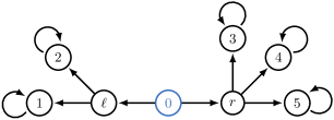
Figure 11: ${\color[rgb]{.25,.45,.75}s_{0}}$ is the starting state, and $\left|\mathcal{A}\right|=10^{10^{10}}$. At ${\color[rgb]{.25,.45,.75}s_{0}}$, half of the actions lead to $s_{\ell}$, while the other half lead to $s_{r}$. Similarly, half of the actions at $s_{\ell}$ lead to $s_{1}$, while the other half lead to $s_{2}$. At $s_{r}$, one action leads to $s_{3}$, one action leads to $s_{4}$, and the remaining $10^{10^{10}}-2$ actions lead to $s_{5}$.

Consider a model-based RL agent with black-box simulator access to this environment. The agent has no prior information about the model, and so it acts randomly. Before long, the agent has probably learned how to navigate from ${\color[rgb]{.25,.45,.75}s_{0}}$ to states $s_{\ell}$, $s_{r}$, $s_{1}$, $s_{2}$, and $s_{5}$. However, over any reasonable timescale, it is extremely improbable that the agent discovers the two actions respectively leading to $s_{3}$ and $s_{4}$.

Even provided with a reward function $R$ and the discount rate $\gamma$, the agent has yet to learn the relevant environmental dynamics, and so many of its policies are far from optimal. Although 6.6 shows that $\forall\gamma\in[0,1]\mathrel{\mathop{\ordinarycolon}}\text{{Power}}_{\mathcal{D}_{\text{bound}}}\left(s_{\ell},\gamma\right)\leq_{\text{{most}}\text{: }\mathfrak{D}_{\text{bound}}}\text{{Power}}_{\mathcal{D}_{\text{bound}}}\left(s_{r},\gamma\right)$, there is a sense in which $s_{\ell}$ gives this agent more power.

We formalize a bounded agent’s goal-achievement capabilities with a function pol, which takes as input a reward function and a discount rate, and returns a policy. Informally, this is the best policy which the agent knows about. We can then calculate $\text{{Power}}_{\mathcal{D}_{\text{bound}}}$ with respect to pol.

Definition C.1 (Suboptimal Power).

Let $\Pi_{\Delta}$ be the set of stationary stochastic policies, and let $\text{pol}\mathrel{\mathop{\ordinarycolon}}\mathbb{R}^{\mathcal{S}}\times[0,1]\to\Pi_{\Delta}$. For $\gamma\in[0,1]$,

$$\text{{Power}}^{\text{pol}}_{\mathcal{D}_{\text{bound}}}\left(s,\gamma\right)\coloneqq\operatorname*{\mathbb{E}}_{\begin{subarray}{c}R\sim\mathcal{D}_{\text{bound}},\\ a\sim\text{pol}\left(R,\gamma\right)(s),\\ s^{\prime}\sim T\left(s,a\right)\end{subarray}}\left[\lim_{\gamma^{*}\to\gamma}(1-\gamma^{*})V^{\text{pol}\left(R,\gamma\right)}_{R}\left(s^{\prime},\gamma^{*}\right)\right].$$ (5)

By E.36, $\text{{Power}}_{\mathcal{D}_{\text{bound}}}$ is the special case where $\forall R\in\mathbb{R}^{\mathcal{S}},\gamma\in[0,1]\mathrel{\mathop{\ordinarycolon}}\text{pol}\left(R,\gamma\right)\in\Pi^{*}\left(R,\gamma\right)$. We define $\text{{Power}}^{\text{pol}}_{\mathcal{D}_{\text{bound}}}$-seeking similarly as in definition 5.6.

$\text{{Power}}^{\text{pol}}_{\mathcal{D}_{\text{bound}}}\left({\color[rgb]{.25,.45,.75}s_{0}},1\right)$ increases as the policies returned by pol are improved. We illustrate this by considering the $\mathcal{D}_{X\text{-}\textsc{iid}}$ case.

1. The model is initially unknown, and so $\forall R,\gamma\mathrel{\mathop{\ordinarycolon}}\text{pol}_{1}(R,\gamma)$ is a uniformly random policy. Since $\text{pol}_{1}$ is constant on its inputs, $\text{{Power}}^{\text{pol}_{1}}_{\mathcal{D}_{X\text{-}\textsc{iid}}}\left({\color[rgb]{.25,.45,.75}s_{0}},1\right)=\operatorname*{\mathbb{E}}\left[X\right]$ by the linearity of expectation and the fact that $\mathcal{D}_{X\text{-}\textsc{iid}}$ distributes reward independently and identically across states.

2. The agent knows the dynamics, except that it does not know how to reach $s_{3}$ or $s_{4}$. At this point, $\text{pol}_{2}(R,1)$ navigates from ${\color[rgb]{.25,.45,.75}s_{0}}$ to the average-optimal choice among three terminal states: $s_{1}$, $s_{2}$, and $s_{5}$. Therefore, $\text{{Power}}^{\text{pol}_{2}}_{\mathcal{D}_{\text{bound}}}\left({\color[rgb]{.25,.45,.75}s_{0}},1\right)=\operatorname*{\mathbb{E}}\left[\max\text{ of }3\text{ draws from }X\right]$.

3. The agent knows the dynamics, the environment is small enough to solve explicitly, and so $\forall R,\gamma\mathrel{\mathop{\ordinarycolon}}\text{pol}_{3}(R,\gamma)$ is an optimal policy. $\text{pol}_{3}(R,1)$ navigates from ${\color[rgb]{.25,.45,.75}s_{0}}$ to the average-optimal choice among all five terminal states. Therefore, $\text{{Power}}^{\text{pol}_{3}}_{\mathcal{D}_{\text{bound}}}\left({\color[rgb]{.25,.45,.75}s_{0}},1\right)=\operatorname*{\mathbb{E}}\left[\max\text{ of }5\text{ draws from }X\right]$.

As the agent learns more about the environment and improves pol, the agent’s $\text{{Power}}^{\text{pol}}_{\mathcal{D}_{\text{bound}}}$ increases. The agent seeks $\text{{Power}}^{\text{pol}_{2}}_{\mathcal{D}_{\text{bound}}}$ by navigating to $s_{\ell}$ instead of $s_{r}$, but seeks more $\text{{Power}}_{\mathcal{D}_{\text{bound}}}$ by navigating to $s_{r}$ instead of $s_{\ell}$. Intuitively, bounded agents gain power by improving pol and by formally seeking $\text{{Power}}^{\text{pol}}_{\mathcal{D}_{\text{bound}}}$ within the environment.

Appendix D Lists of results

List of definitions

1. Definition 3.1 (Rewardless mdp).
2. Definition 3.2 (1-cycle states).
3. Definition 3.3 (State visit distribution [Sutton and Barto, 1998]).
4. Definition 3.4 ($\operatorname{\mathcal{F}}$ single-state restriction).
5. Definition 3.5 (Value function).
6. Definition 3.6 (Non-domination).
7. Definition 4.1 (Optimal policy set function).
8. Definition 4.2 (Reward function distributions).
9. Definition 4.3 (Visit distribution optimality probability).
10. Definition 4.4 (Action optimality probability).
11. Definition 5.1 (Average optimal value).
12. Definition 5.2 (Power).
13. Definition 5.6 (Power-seeking actions).
14. Definition 6.1 (Similarity of vector sets).
15. Definition 6.2 (Similarity of vector function sets).
16. Definition 6.3 (Pushforward distribution of a permutation).
17. Definition 6.4 (Orbit of a probability distribution).
18. Definition 6.5 (Inequalities which hold for most probability distributions).
19. Definition 6.7 (Equivalent actions).
20. Definition 6.8 (States reachable after taking an action).
21. Definition 6.10 (Recurrent state distributions [Puterman, 2014]).
22. Definition 6.11 (Average-optimal policies).
23. Definition C.1 (Suboptimal Power).
24. Definition E.2 (Transition matrix induced by a policy).
25. Definition E.6 (Continuous reward function distribution).
26. Definition E.9 (Non-dominated linear functionals).
27. Definition E.13 (Non-dominated vector functions).
28. Definition E.14 (Affine transformation of visit distribution sets).
29. Definition E.18 (Support of $\mathcal{D}_{\text{any}}$).
30. Definition E.19 (Linear functional optimality probability).
31. Definition E.23 (Bounded, continuous iid reward).
32. Definition E.25 (Indicator function).
33. Definition E.30 (Evaluating sets of visit distribution functions at $\gamma$).
34. Definition E.37 (Discount-normalized value function).
35. Definition E.40 (Normalized visit distribution function).

cor-no-num,conjecture,remark,definition

List of theorems

1. Definition 3.1 (Rewardless mdp).
2. Definition 3.2 (1-cycle states).
3. Definition 3.3 (State visit distribution [Sutton and Barto, 1998]).
4. Definition 3.4 ($\operatorname{\mathcal{F}}$ single-state restriction).
5. Definition 3.5 (Value function).
6. Definition 3.6 (Non-domination).
7. Definition 4.1 (Optimal policy set function).
8. Definition 4.2 (Reward function distributions).
9. Definition 4.3 (Visit distribution optimality probability).
10. Definition 4.4 (Action optimality probability).
11. Definition 5.1 (Average optimal value).
12. Definition 5.2 (Power).
13. Lemma 5.3 (Continuity of Power).
14. Proposition 5.4 (Maximal Power).
15. Proposition 5.5 (Power is smooth across reversible dynamics).
16. Definition 5.6 (Power-seeking actions).
17. Definition 6.1 (Similarity of vector sets).
18. Definition 6.2 (Similarity of vector function sets).
19. Definition 6.3 (Pushforward distribution of a permutation).
20. Definition 6.4 (Orbit of a probability distribution).
21. Definition 6.5 (Inequalities which hold for most probability distributions).
22. Proposition 6.6 (States with “more options” have more Power).
23. Definition 6.7 (Equivalent actions).
24. Definition 6.8 (States reachable after taking an action).
25. Proposition 6.9 (Keeping options open tends to be Power-seeking and tends to be optimal).
26. Definition 6.10 (Recurrent state distributions [Puterman, 2014]).
27. Definition 6.11 (Average-optimal policies).
28. Proposition 6.12 (When $\gamma=1$, rsds control Power).
29. Theorem 6.13 (Average-optimal policies tend to end up in “larger” sets of rsds).
30. Corollary 6.14 (Average-optimal policies tend not to end up in any given 1-cycle).
31. Remark.
32. Proposition B.1 (Greater $\text{{Power}}_{\mathcal{D}_{\text{bound}}}$ does not imply greater $\operatorname*{\mathbb{P}}_{\mathcal{D}_{\text{bound}}}$).
33. Lemma B.2 (Fraction of orbits which agree on weak optimality).
34. Lemma B.3 ($\geq_{\text{most}}$ and trivial orbits).
35. Proposition B.4 (Actions which tend to seek Power do not necessarily tend to be optimal).
36. Definition C.1 (Suboptimal Power).
37. Lemma E.1 (A policy is optimal iff it induces an optimal visit distribution at every state).
38. Definition E.2 (Transition matrix induced by a policy).
39. Proposition E.3 (Properties of visit distribution functions).
40. Lemma E.4 ($\mathbf{f}\in\operatorname{\mathcal{F}}(s)$ is multivariate rational on $\gamma$).
41. Corollary E.5 (On-policy value is rational on $\gamma$).
42. Definition E.6 (Continuous reward function distribution).
43. Remark.
44. Lemma E.7 (Distinct linear functionals disagree almost everywhere on their domains).
45. Corollary E.8 (Unique maximization of almost all vectors).
46. Definition E.9 (Non-dominated linear functionals).
47. Lemma E.10 (All vectors are maximized by a non-dominated linear functional).
48. Corollary E.11 (Maximal value is invariant to restriction to non-dominated functionals).
49. Lemma E.12 (How non-domination containment affects optimal value).
50. Definition E.13 (Non-dominated vector functions).
51. Remark.
52. Definition E.14 (Affine transformation of visit distribution sets).
53. Lemma E.15 (Invariance of non-domination under positive affine transform).
54. Lemma E.16 (Helper lemma for demonstrating $\geq_{\text{{most}}\text{: }\mathfrak{D}_{\text{any}}}$).
55. Lemma E.17 (A helper result for expectations of functions).
56. Definition E.18 (Support of $\mathcal{D}_{\text{any}}$).
57. Definition E.19 (Linear functional optimality probability).
58. Proposition E.20 (Non-dominated linear functionals and their optimality probability).
59. Lemma E.21 (Expected value of similar linear functional sets).
60. Lemma E.22 (For continuous iid distributions $\mathcal{D}_{X\text{-}\textsc{iid}}$, $\exists b<c\mathrel{\mathop{\ordinarycolon}}(b,c)^{\left|\mathcal{S}\right|}\subseteq\operatorname{supp}(\mathcal{D}_{X\text{-}\textsc{iid}})$).
61. Definition E.23 (Bounded, continuous iid reward).
62. Lemma E.24 (Expectation superiority lemma).
63. Definition E.25 (Indicator function).
64. Lemma E.26 (Optimality probability inclusion relations).
65. Lemma E.27 (Optimality probability of similar linear functional sets).
66. Lemma E.28 (Optimality probability superiority lemma).
67. Lemma E.29 (Limit probability inequalities which hold for most distributions).
68. Definition E.30 (Evaluating sets of visit distribution functions at $\gamma$).
69. Lemma E.31 (Non-domination across $\gamma$ values for expectations of visit distributions).
70. Lemma E.32 ($\forall\gamma\in(0,1)\mathrel{\mathop{\ordinarycolon}}\mathbf{d}\in\operatorname{\mathcal{F}_{nd}}(s,\gamma)$ iff $\mathbf{d}\in\text{{ND}}\left(\operatorname{\mathcal{F}}(s,\gamma)\right)$).
71. Lemma E.33 (Optimal policy shift bound).
72. Proposition E.34 (Optimality probability’s limits exist).
73. Lemma E.35 (Optimality probability identity).
74. Lemma E.36 (Power identities).
75. Definition E.37 (Discount-normalized value function).
76. Lemma E.38 (Normalized value functions have uniformly bounded derivative).
77. Lemma E.39 (Lower bound on current Power based on future Power).
78. Definition E.40 (Normalized visit distribution function).
79. Remark.
80. Lemma E.41 (Normalized visit distribution functions are continuous).
81. Lemma E.42 (Non-domination of normalized visit distribution functions).
82. Lemma E.43 (Power limit identity).
83. Lemma E.44 (Lemma for Power superiority).
84. Lemma E.45 (Non-dominated visit distribution functions never agree with other visit distribution functions at that state).
85. Corollary E.46 (Cardinality of non-dominated visit distributions).
86. Lemma E.47 (Optimality probability and state bottlenecks).
87. Lemma E.48 (Action optimality probability is a special case of visit distribution optimality probability).
88. Lemma E.49 (Power identity when $\gamma=1$).
89. Proposition E.50 (Rsd properties).
90. Lemma E.51 (When reachable with probability 1, 1-cycles induce non-dominated rsds).

D.1 Contributions of independent interest

We developed new basic mdp theory by exploring the structural properties of visit distribution functions. Echoing Wang et al. [2007, 2008], we believe that this area is interesting and underexplored.

D.1.1 Optimal value theory

E.38 shows that $f(\gamma^{*})\coloneqq\lim_{\gamma^{*}\to\gamma}(1-\gamma^{*})V^{*}_{R}\left(s,\gamma^{*}\right)$ is Lipschitz continuous on $\gamma\in[0,1]$, with Lipschitz constant depending only on $\left\lVert R\right\rVert_{1}$. For all states $s$ and policies $\pi\in\Pi$, E.5 shows that $V^{\pi}_{R}(s,\gamma)$ is rational on $\gamma$.

Optimal value has a well-known dual formulation: $V^{*}_{R}\left(s,\gamma\right)=\max_{\mathbf{f}\in\operatorname{\mathcal{F}}(s)}\mathbf{f}(\gamma)^{\top}\mathbf{r}$. [$\forall\gamma\in[0,1)\mathrel{\mathop{\ordinarycolon}}V^{*}_{R}\left(s,\gamma\right)=\max_{\mathbf{f}\in\operatorname{\mathcal{F}_{nd}}(s)}\mathbf{f}(\gamma)^{\top}\mathbf{r}$]lemoptVfFndRestrict In a fixed rewardless mdp, section D.1.1 may enable more efficient computation of optimal value functions for multiple reward functions.

D.1.2 Optimal policy theory

Section D.1.2 demonstrates how to preserve optimal incentives while changing the discount rate.

[How to transfer optimal policy sets across discount rates]proptransferDiscount Suppose reward function $R$ has optimal policy set $\Pi^{*}\left(R,\gamma\right)$ at discount rate $\gamma\in(0,1)$. For any $\gamma^{*}\in(0,1)$, we can construct a reward function $R^{\prime}$ such that $\Pi^{*}\left(R^{\prime},\gamma^{*}\right)=\Pi^{*}\left(R,\gamma\right)$. Furthermore, $V^{*}_{R^{\prime}}\left(\cdot,\gamma^{*}\right)=V^{*}_{R}\left(\cdot,\gamma\right)$.

D.1.3 Visit distribution theory

While Regan and Boutilier [2010] consider a visit distribution function $\mathbf{f}\in\operatorname{\mathcal{F}}(s)$ to be non-dominated if it is optimal for some reward function in a set $\mathcal{R}_{\text{}}\subseteq\mathbb{R}^{\left|\mathcal{S}\right|}$, our stricter definition 3.6 considers $\mathbf{f}$ to be non-dominated when $\exists\mathbf{r}\in\mathbb{R}^{\left|\mathcal{S}\right|},\gamma\in(0,1)\mathrel{\mathop{\ordinarycolon}}\mathbf{f}(\gamma)^{\top}\mathbf{r}>\max_{\mathbf{f}^{\prime}\in\operatorname{\mathcal{F}}(s)\setminus\left\{\mathbf{f}\right\}}\mathbf{f}^{\prime}(\gamma)^{\top}\mathbf{r}$.

Appendix E Theoretical results

Lemma E.1 (A policy is optimal iff it induces an optimal visit distribution at every state).

Let $\gamma\in(0,1)$ and let $R$ be a reward function. $\pi\in\Pi^{*}\left(R,\gamma\right)$ iff $\pi$ induces an optimal visit distribution at every state.

Proof.

By definition, a policy $\pi$ is optimal iff $\pi$ induces the maximal on-policy value at each state, which is true iff $\pi$ induces an optimal visit distribution at every state (by the dual formulation of optimal value functions). ∎

Definition E.2 (Transition matrix induced by a policy).

$\mathbf{T}^{\pi}$ is the transition matrix induced by policy $\pi\in\Pi$, where $\mathbf{T}^{\pi}\mathbf{e}_{s}\coloneqq T(s,\pi(s))$. $(\mathbf{T}^{\pi})^{t}\mathbf{e}_{s}$ gives the probability distribution over the states visited at time step $t$, after following $\pi$ for $t$ steps from $s$.

Proposition E.3 (Properties of visit distribution functions).

Let $s,s^{\prime}\in\mathcal{S},\mathbf{f}^{\pi,s}\in\operatorname{\mathcal{F}}(s)$.

1. $\mathbf{f}^{\pi,s}(\gamma)$ is element-wise non-negative and element-wise monotonically increasing on $\gamma\in[0,1)$.

2. $\forall\gamma\in[0,1)\mathrel{\mathop{\ordinarycolon}}\left\lVert\mathbf{f}^{\pi,s}(\gamma)\right\rVert_{1}=\frac{1}{1-\gamma}$.

Proof.

Item 1: by examination of definition 3.3, $\mathbf{f}^{\pi,s}=\sum_{t=0}^{\infty}\left(\gamma\mathbf{T}^{\pi}\right)^{t}\mathbf{e}_{s}$. Since each $\left(\mathbf{T}^{\pi}\right)^{t}$ is left stochastic and $\mathbf{e}_{s}$ is the standard unit vector, each entry in each summand is non-negative. Therefore, $\forall\gamma\in[0,1)\mathrel{\mathop{\ordinarycolon}}\mathbf{f}^{\pi,s}(\gamma)^{\top}\mathbf{e}_{s^{\prime}}\geq 0$, and this function monotonically increases on $\gamma$.

Item 2:

$$\left\lVert\mathbf{f}^{\pi,s}(\gamma)\right\rVert_{1} =\left\lVert\sum_{t=0}^{\infty}\left(\gamma\mathbf{T}^{\pi}\right)^{t}\mathbf{e}_{s}\right\rVert_{1}$$ (6)

$$=\sum_{t=0}^{\infty}\gamma^{t}\left\lVert\left(\mathbf{T}^{\pi}\right)^{t}\mathbf{e}_{s}\right\rVert_{1}$$ (7)

$$=\sum_{t=0}^{\infty}\gamma^{t}$$ (8)

$$=\frac{1}{1-\gamma}.$$ (9)

Equation 7 follows because all entries in each $\left(\mathbf{T}^{\pi}\right)^{t}\mathbf{e}_{s}$ are non-negative by item 1. Equation 8 follows because each $\left(\mathbf{T}^{\pi}\right)^{t}$ is left stochastic and $\mathbf{e}_{s}$ is a stochastic vector, and so $\left\lVert\left(\mathbf{T}^{\pi}\right)^{t}\mathbf{e}_{s}\right\rVert_{1}=1$. ∎

Lemma E.4 ($\mathbf{f}\in\operatorname{\mathcal{F}}(s)$ is multivariate rational on $\gamma$).

$\mathbf{f}^{\pi}\in\operatorname{\mathcal{F}}(s)$ is a multivariate rational function on $\gamma\in[0,1)$.

Proof.

Let $\mathbf{r}\in\mathbb{R}^{\left|\mathcal{S}\right|}$ and consider $\mathbf{f}^{\pi}\in\operatorname{\mathcal{F}}(s)$. Let $\mathbf{v}^{\pi}_{R}$ be the $V^{*}_{R}\left(s,\gamma\right)$ function in column vector form, with one entry per state value.

By the Bellman equations, $\mathbf{v}^{\pi}_{R}=\left(\mathbf{I}-\gamma\mathbf{T}^{\pi}\right)^{-1}\mathbf{r}.$ Let $\mathbf{A}_{\gamma}\coloneqq\left(\mathbf{I}-\gamma\mathbf{T}^{\pi}\right)^{-1}$, and for state $s$, form $\mathbf{A}_{s,\gamma}$ by replacing $\mathbf{A}_{\gamma}$’s column for state $s$ with $\mathbf{r}$. As noted by Lippman [1968], by Cramer’s rule, $V^{\pi}_{R}(s,\gamma)=\frac{\det{\mathbf{A}_{s,\gamma}}}{\det\mathbf{A}_{\gamma}}$ is a rational function with numerator and denominator having degree at most $\left|\mathcal{S}\right|$.

In particular, for each state indicator reward function $\mathbf{e}_{s_{i}}$, $V^{\pi}_{s_{i}}(s,\gamma)=\mathbf{f}^{\pi,s}(\gamma)^{\top}\mathbf{e}_{s_{i}}$ is a rational function of $\gamma$ whose numerator and denominator each have degree at most $\left|\mathcal{S}\right|$. This implies that $\mathbf{f}^{\pi}(\gamma)$ is multivariate rational on $\gamma\in[0,1)$. ∎

Corollary E.5 (On-policy value is rational on $\gamma$).

Let $\pi\in\Pi$ and $R$ be any reward function. $V^{\pi}_{R}(s,\gamma)$ is rational on $\gamma\in[0,1)$.

Proof.

$V^{\pi}_{R}(s,\gamma)=\mathbf{f}^{\pi,s}(\gamma)^{\top}\mathbf{r}$, and $\mathbf{f}$ is a multivariate rational function of $\gamma$ by E.4. Therefore, for fixed $\mathbf{r}$, $\mathbf{f}^{\pi,s}(\gamma)^{\top}\mathbf{r}$ is a rational function of $\gamma$. ∎

E.1 Non-dominated visit distribution functions

Definition E.6 (Continuous reward function distribution).

Results with $\mathcal{D}_{\text{cont}}$ hold for any absolutely continuous reward function distribution.

Remark.

We assume $\mathbb{R}^{\left|\mathcal{S}\right|}$ is endowed with the standard topology.

Lemma E.7 (Distinct linear functionals disagree almost everywhere on their domains).

Let $\mathbf{x},\mathbf{x}^{\prime}\in\mathbb{R}^{\left|\mathcal{S}\right|}$ be distinct. $\operatorname*{\mathbb{P}}\nolimits_{\mathbf{r}\sim\mathcal{D}_{\text{cont}}}\left(\mathbf{x}^{\top}\mathbf{r}=\mathbf{x}^{\prime\top}\mathbf{r}\right)=0$.

Proof.

$\left\{\mathbf{r}\in\mathbb{R}^{\left|\mathcal{S}\right|}\mid(\mathbf{x}-\mathbf{x}^{\prime})^{\top}\mathbf{r}=0\right\}$ is a hyperplane since $\mathbf{x}-\mathbf{x}^{\prime}\neq\mathbf{0}$. Therefore, it has no interior in the standard topology on $\mathbb{R}^{\left|\mathcal{S}\right|}$. Since this empty-interior set is also convex, it has zero Lebesgue measure. By the Radon-Nikodym theorem, it has zero measure under any continuous distribution $\mathcal{D}_{\text{cont}}$. ∎

Corollary E.8 (Unique maximization of almost all vectors).

Let $X\subsetneq\mathbb{R}^{\left|\mathcal{S}\right|}$ be finite. $\operatorname*{\mathbb{P}}\nolimits_{\mathbf{r}\sim\mathcal{D}_{\text{cont}}}\left(\left|\operatorname*{arg\,max}_{\mathbf{x}^{\prime\prime}\in X}\mathbf{x}^{\prime\prime\top}\mathbf{r}\right|>1\right)=0$.

Proof.

Let $\mathbf{x},\mathbf{x}^{\prime}\in X$ be distinct. For any $\mathbf{r}\in\mathbb{R}^{\left|\mathcal{S}\right|}$, $\mathbf{x},\mathbf{x}^{\prime}\in\operatorname*{arg\,max}_{\mathbf{x}^{\prime\prime}\in X}\mathbf{x}^{\prime\prime\top}\mathbf{r}$ iff $\mathbf{x}^{\top}\mathbf{r}=\mathbf{x}^{\prime\top}\mathbf{r}\geq\max_{\mathbf{x}^{\prime\prime}\in X\setminus\left\{\mathbf{x},\mathbf{x}^{\prime}\right\}}\mathbf{x}^{\prime\prime\top}\mathbf{r}$. By E.7, $\mathbf{x}^{\top}\mathbf{r}=\mathbf{x}^{\prime\top}\mathbf{r}$ holds with probability 0 under any $\mathcal{D}_{\text{cont}}$. ∎

E.1.1 Generalized non-domination results

Our formalism includes both $\operatorname{\mathcal{F}_{nd}}(s)$ and $\text{{RSD}}{\text{\textsubscript{nd}}}\left(s\right)$; we therefore prove results that are applicable to both.

Definition E.9 (Non-dominated linear functionals).

Let $X\subsetneq\mathbb{R}^{\left|\mathcal{S}\right|}$ be finite. $\text{{ND}}\left(X\right)\coloneqq\left\{\mathbf{x}\in X\mid\exists\mathbf{r}\in\mathbb{R}^{\left|\mathcal{S}\right|}\mathrel{\mathop{\ordinarycolon}}\mathbf{x}^{\top}\mathbf{r}>\max_{\mathbf{x}^{\prime}\in X\setminus\left\{\mathbf{x}\right\}}\mathbf{x}^{\prime\top}\mathbf{r}\right\}$.

Lemma E.10 (All vectors are maximized by a non-dominated linear functional).

Let $\mathbf{r}\in\mathbb{R}^{\left|\mathcal{S}\right|}$ and let $X\subsetneq\mathbb{R}^{\left|\mathcal{S}\right|}$ be finite and non-empty. $\exists\mathbf{x}^{*}\in\text{{ND}}\left(X\right)\mathrel{\mathop{\ordinarycolon}}\mathbf{x}^{*\top}\mathbf{r}=\max_{\mathbf{x}\in X}\mathbf{x}^{\top}\mathbf{r}$.

Proof.

Let $A(\mathbf{r}\mid X)\coloneqq\operatorname*{arg\,max}_{\mathbf{x}\in X}\mathbf{x}^{\top}\mathbf{r}=\left\{\mathbf{x}_{1},\ldots,\mathbf{x}_{n}\right\}$. Then

$$\mathbf{x}_{1}^{\top}\mathbf{r}=\cdots=\mathbf{x}_{n}^{\top}\mathbf{r}>\max_{\mathbf{x}^{\prime}\in X\setminus A(\mathbf{r}\mid X)}\mathbf{x}^{\prime\top}\mathbf{r}.$$ (10)

In eq. 10, each $\mathbf{x}^{\top}\mathbf{r}$ expression is linear on $\mathbf{r}$. The $\max$ is piecewise linear on $\mathbf{r}$ since it is the maximum of a finite set of linear functionals. In particular, all expressions in eq. 10 are continuous on $\mathbf{r}$, and so we can find some $\delta>0$ neighborhood $B(\mathbf{r},\delta)$ such that $\forall\mathbf{r}^{\prime}\in B(\mathbf{r},\delta)\mathrel{\mathop{\ordinarycolon}}\max_{\mathbf{x}_{i}\in A(\mathbf{r}\mid X)}\mathbf{x}_{i}^{\top}\mathbf{r}^{\prime}>\max_{\mathbf{x}^{\prime}\in X\setminus A(\mathbf{r}\mid X)}\mathbf{x}^{\prime\top}\mathbf{r}^{\prime}$.

But almost all $\mathbf{r}^{\prime}\in B(\mathbf{r},\delta)$ are maximized by a unique functional $\mathbf{x}^{*}$ by E.8; in particular, at least one such $\mathbf{r}^{\prime\prime}$ exists. Formally, $\exists\mathbf{r}^{\prime\prime}\in B(\mathbf{r},\delta)\mathrel{\mathop{\ordinarycolon}}\mathbf{x}^{*\top}\mathbf{r}^{\prime\prime}>\max_{\mathbf{x}^{\prime}\in X\setminus\left\{\mathbf{x}^{*}\right\}}\mathbf{x}^{\prime\top}\mathbf{r}^{\prime\prime}$. Therefore, $\mathbf{x}^{*}\in\text{{ND}}\left(X\right)$ by definition E.9.

$\mathbf{x}^{*\top}\mathbf{r}^{\prime}\geq\max_{\mathbf{x}_{i}\in A(\mathbf{r}\mid X)}\mathbf{x}_{i}^{\top}\mathbf{r}^{\prime}>\max_{\mathbf{x}^{\prime}\in X\setminus A(\mathbf{r}\mid X)}\mathbf{x}^{\prime\top}\mathbf{r}^{\prime}$, with the strict inequality following because $\mathbf{r}^{\prime\prime}\in B(\mathbf{r},\delta)$. These inequalities imply that $\mathbf{x}^{*}\in A(\mathbf{r}\mid X)$. ∎

Corollary E.11 (Maximal value is invariant to restriction to non-dominated functionals).

Let $\mathbf{r}\in\mathbb{R}^{\left|\mathcal{S}\right|}$ and let $X\subsetneq\mathbb{R}^{\left|\mathcal{S}\right|}$ be finite. $\max_{\mathbf{x}\in X}\mathbf{x}^{\top}\mathbf{r}=\max_{\mathbf{x}\in\text{{ND}}\left(X\right)}\mathbf{x}^{\top}\mathbf{r}$.

Proof.

If $X$ is empty, holds trivially. Otherwise, apply E.10. ∎

Lemma E.12 (How non-domination containment affects optimal value).

Let $\mathbf{r}\in\mathbb{R}^{\left|\mathcal{S}\right|}$ and let $X,X^{\prime}\subsetneq\mathbb{R}^{\left|\mathcal{S}\right|}$ be finite.

1. If $\text{{ND}}\left(X\right)\subseteq X^{\prime}$, then $\max_{\mathbf{x}\in X}\mathbf{x}^{\top}\mathbf{r}\leq\max_{\mathbf{x}^{\prime}\in X^{\prime}}\mathbf{x}^{\prime\top}\mathbf{r}$.

2. If $\text{{ND}}\left(X\right)\subseteq X^{\prime}\subseteq X$, then $\max_{\mathbf{x}\in X}\mathbf{x}^{\top}\mathbf{r}=\max_{\mathbf{x}^{\prime}\in X^{\prime}}\mathbf{x}^{\prime\top}\mathbf{r}$.

Proof.

Item 1:

$$\max_{\mathbf{x}\in X}\mathbf{x}^{\top}\mathbf{r} =\max_{\mathbf{x}\in\text{{ND}}\left(X\right)}\mathbf{x}^{\top}\mathbf{r}$$ (11)

$$\leq\max_{\mathbf{x}^{\prime}\in X^{\prime}}\mathbf{x}^{\prime\top}\mathbf{r}.$$ (12)

Equation 11 follows by E.11. Equation 12 follows because $\text{{ND}}\left(X\right)\subseteq X^{\prime}$.

Item 2: by item 1, $\max_{\mathbf{x}\in X}\mathbf{x}^{\top}\mathbf{r}\leq\max_{\mathbf{x}^{\prime}\in X^{\prime}}\mathbf{x}^{\prime\top}\mathbf{r}$. Since $X^{\prime}\subseteq X$, we also have $\max_{\mathbf{x}\in X}\mathbf{x}^{\top}\mathbf{r}\geq\max_{\mathbf{x}^{\prime}\in X^{\prime}}\mathbf{x}^{\prime\top}\mathbf{r}$, and so equality must hold. ∎

Definition E.13 (Non-dominated vector functions).

Let $I\subseteq\mathbb{R}$ and let $F\subsetneq\left(\mathbb{R}^{\left|\mathcal{S}\right|}\right)^{I}$ be a finite set of vector-valued functions on $I$. $\text{{ND}}\left(F\right)\coloneqq\left\{\mathbf{f}\in F\mid\exists\gamma\in I,\mathbf{r}\in\mathbb{R}^{\left|\mathcal{S}\right|}\mathrel{\mathop{\ordinarycolon}}\mathbf{f}(\gamma)^{\top}\mathbf{r}>\max_{\mathbf{f}^{\prime}\in F\setminus\left\{\mathbf{f}\right\}}\mathbf{f}^{\prime}(\gamma)^{\top}\mathbf{r}\right\}$.

Remark.

$\operatorname{\mathcal{F}_{nd}}(s)=\text{{ND}}\left(\operatorname{\mathcal{F}}(s)\right)$ by definition 3.6.

Definition E.14 (Affine transformation of visit distribution sets).

For notational convenience, we define set-scalar multiplication and set-vector addition on $X\subseteq\mathbb{R}^{\left|\mathcal{S}\right|}$: for $c\in\mathbb{R}$, $cX\coloneqq\left\{c\mathbf{x}\mid\mathbf{x}\in X\right\}$. For $\mathbf{a}\in\mathbb{R}^{\left|\mathcal{S}\right|}$, $X+\mathbf{a}\coloneqq\left\{\mathbf{x}+\mathbf{a}\mid\mathbf{x}\in X\right\}$. Similar operations hold when $X$ is a set of vector functions $\mathbb{R}\mapsto\mathbb{R}^{\left|\mathcal{S}\right|}$.

Lemma E.15 (Invariance of non-domination under positive affine transform).

1. Let $X\subsetneq\mathbb{R}^{\left|\mathcal{S}\right|}$ be finite. If $\mathbf{x}\in\text{{ND}}\left(X\right)$, then $\forall c>0,\mathbf{a}\in\mathbb{R}^{\left|\mathcal{S}\right|}\mathrel{\mathop{\ordinarycolon}}(c\mathbf{x}+\mathbf{a})\in\text{{ND}}\left(cX+\mathbf{a}\right)$.

2. Let $I\subseteq\mathbb{R}$ and let $F\subsetneq\left(\mathbb{R}^{\left|\mathcal{S}\right|}\right)^{I}$ be a finite set of vector-valued functions on $I$. If $\mathbf{f}\in\text{{ND}}\left(F\right)$, then $\forall c>0,\mathbf{a}\in\mathbb{R}^{\left|\mathcal{S}\right|}\mathrel{\mathop{\ordinarycolon}}(c\mathbf{f}+\mathbf{a})\in\text{{ND}}\left(cF+\mathbf{a}\right)$.

Proof.

Item 1: Suppose $\mathbf{x}\in\text{{ND}}\left(X\right)$ is strictly optimal for $\mathbf{r}\in\mathbb{R}^{\left|\mathcal{S}\right|}$. Then let $c>0,\mathbf{a}\in\mathbb{R}^{\left|\mathcal{S}\right|}$ be arbitrary, and define $b\coloneqq\mathbf{a}^{\top}\mathbf{r}$.

$$\mathbf{x}^{\top}\mathbf{r} >\max_{\mathbf{x}^{\prime}\in X\setminus\left\{\mathbf{x}\right\}}\mathbf{x}^{\prime\top}\mathbf{r}$$ (13)

$$c\mathbf{x}^{\top}\mathbf{r}+b >\max_{\mathbf{x}^{\prime}\in X\setminus\left\{\mathbf{x}\right\}}c\mathbf{x}^{\prime\top}\mathbf{r}+b$$ (14)

$$(c\mathbf{x}+\mathbf{a})^{\top}\mathbf{r} >\max_{\mathbf{x}^{\prime}\in X\setminus\left\{\mathbf{x}\right\}}(c\mathbf{x}^{\prime}+\mathbf{a})^{\top}\mathbf{r}$$ (15)

$$(c\mathbf{x}+\mathbf{a})^{\top}\mathbf{r} >\max_{\mathbf{x}^{\prime\prime}\in\left(cX+\mathbf{a}\right)\setminus\left\{c\mathbf{x}+\mathbf{a}\right\}}\mathbf{x}^{\prime\prime\top}\mathbf{r}.$$ (16)

Equation 14 follows because $c>0$. Equation 15 follows by the definition of $b$.

Item 2: If $\mathbf{f}\in\text{{ND}}\left(F\right)$, then by definition E.13, there exist $\gamma\in I,\mathbf{r}\in\mathbb{R}^{\left|\mathcal{S}\right|}$ such that

$$\mathbf{f}(\gamma)^{\top}\mathbf{r}>\max_{\mathbf{f}^{\prime}\in F\setminus\left\{\mathbf{f}\right\}}\mathbf{f}^{\prime}(\gamma)^{\top}\mathbf{r}.$$ (17)

Apply item 1 to conclude

$$(c\mathbf{f}(\gamma)+\mathbf{a})^{\top}\mathbf{r}>\max_{(c\mathbf{f}^{\prime}+\mathbf{a})\in(cF+\mathbf{a})\setminus\left\{c\mathbf{f}+\mathbf{a}\right\}}(c\mathbf{f}^{\prime}(\gamma)+\mathbf{a})^{\top}\mathbf{r}.$$ (18)

Therefore, $(c\mathbf{f}+\mathbf{a})\in\text{{ND}}\left(cF+\mathbf{a}\right)$. ∎

E.1.2 Inequalities which hold under most reward function distributions

See 6.5

Lemma E.16 (Helper lemma for demonstrating $\geq_{\text{{most}}\text{: }\mathfrak{D}_{\text{any}}}$).

Let $\mathfrak{D}\subseteq\Delta(\mathbb{R}^{\left|\mathcal{S}\right|})$. If $\exists\phi\in S_{\left|\mathcal{S}\right|}$ such that for all $\mathcal{D}\in\mathfrak{D}$, $f_{1}\left(\mathcal{D}\right)<f_{2}\left(\mathcal{D}\right)$ implies that $f_{1}\left(\phi\cdot\mathcal{D}\right)>f_{2}\left(\phi\cdot\mathcal{D}\right)$, then $f_{1}(\mathcal{D})\geq_{\text{{most}}\text{: }\mathfrak{D}}f_{2}(\mathcal{D})$.

Proof.

Since $\phi$ does not belong to the stabilizer of $S_{\left|\mathcal{S}\right|}$, $\phi$ acts injectively on $S_{\left|\mathcal{S}\right|}\cdot\mathcal{D}$. By assumption on $\phi$, the image of $\{\mathcal{D}^{\prime}\in S_{\left|\mathcal{S}\right|}\cdot\mathcal{D}\mid f_{1}(\mathcal{D}^{\prime})<f_{2}(\mathcal{D}^{\prime})\}$ under $\phi$ is a subset of $\{\mathcal{D}^{\prime}\in S_{\left|\mathcal{S}\right|}\cdot\mathcal{D}\mid f_{1}(\mathcal{D}^{\prime})>f_{2}(\mathcal{D}^{\prime})\}$. Since $\phi$ is injective, $\left|\{\mathcal{D}^{\prime}\in S_{\left|\mathcal{S}\right|}\cdot\mathcal{D}\mid f_{1}(\mathcal{D}^{\prime})<f_{2}(\mathcal{D}^{\prime})\}\right|\leq\left|\{\mathcal{D}^{\prime}\in S_{\left|\mathcal{S}\right|}\cdot\mathcal{D}\mid f_{1}(\mathcal{D}^{\prime})>f_{2}(\mathcal{D}^{\prime})\}\right|$. $f_{1}(\mathcal{D})\geq_{\text{{most}}\text{: }\mathfrak{D}}f_{2}(\mathcal{D})$ by definition 6.5. ∎

Lemma E.17 (A helper result for expectations of functions).

Let $B_{1},\ldots,B_{n}\subsetneq\mathbb{R}^{\left|\mathcal{S}\right|}$ be finite and let $\mathfrak{D}\subseteq\Delta(\mathbb{R}^{\left|\mathcal{S}\right|})$. Suppose $f$ is a function of the form

$$f\left(B_{1},\ldots,B_{n}\mid\mathcal{D}\right)=\operatorname*{\mathbb{E}}_{\mathbf{r}\sim\mathcal{D}}\left[g\left(\max_{\mathbf{b}_{1}\in B_{1}}\mathbf{b}_{1}^{\top}\mathbf{r},\ldots,\max_{\mathbf{b}_{n}\in B_{n}}\mathbf{b}_{n}^{\top}\mathbf{r}\right)\right]$$ (19)

for some function $g$, and that $f$ is well-defined for all $\mathcal{D}\in\mathfrak{D}$. Let $\phi$ be a state permutation. Then

$$f\left(B_{1},\ldots,B_{n}\mid\mathcal{D}\right)=f\left(\phi\cdot B_{1},\ldots,\phi\cdot B_{n}\mid\phi\cdot\mathcal{D}\right).$$ (20)

Proof.

Let distribution $\mathcal{D}$ have probability measure $F$, and let $\phi\cdot\mathcal{D}$ have probability measure $F_{\phi}$.

$$f\left(B_{1},\ldots,B_{n}\mid\mathcal{D}\right)$$ (21)

$$\coloneqq{} \operatorname*{\mathbb{E}}_{\mathbf{r}\sim\mathcal{D}}\left[g\left(\max_{\mathbf{b}_{1}\in B_{1}}\mathbf{b}_{1}^{\top}\mathbf{r},\ldots,\max_{\mathbf{b}_{n}\in B_{n}}\mathbf{b}_{n}^{\top}\mathbf{r}\right)\right]$$ (22)

$$\coloneqq{} \int_{\mathbb{R}^{\left|\mathcal{S}\right|}}g\left(\max_{\mathbf{b}_{1}\in B_{1}}\mathbf{b}_{1}^{\top}\mathbf{r},\ldots,\max_{\mathbf{b}_{n}\in B_{n}}\mathbf{b}_{n}^{\top}\mathbf{r}\right)\operatorname{d\!}F(\mathbf{r})$$ (23)

$$={} \int_{\mathbb{R}^{\left|\mathcal{S}\right|}}g\left(\max_{\mathbf{b}_{1}\in B_{1}}\mathbf{b}_{1}^{\top}\mathbf{r},\ldots,\max_{\mathbf{b}_{n}\in B_{n}}\mathbf{b}_{n}^{\top}\mathbf{r}\right)\operatorname{d\!}F_{\phi}(\mathbf{P}_{\phi}\mathbf{r})$$ (24)

$$={} \int_{\mathbb{R}^{\left|\mathcal{S}\right|}}g\left(\max_{\mathbf{b}_{1}\in B_{1}}\mathbf{b}_{1}^{\top}\left(\mathbf{P}_{\phi}^{-1}\mathbf{r}^{\prime}\right),\ldots,\max_{\mathbf{b}_{n}\in B_{n}}\mathbf{b}_{n}^{\top}\left(\mathbf{P}_{\phi}^{-1}\mathbf{r}^{\prime}\right)\right)\left|\det\mathbf{P}_{\phi}\right|\operatorname{d\!}F_{\phi}(\mathbf{r}^{\prime})$$ (25)

$$={} \int_{\mathbb{R}^{\left|\mathcal{S}\right|}}g\left(\max_{\mathbf{b}_{1}\in B_{1}}\left(\mathbf{P}_{\phi}\mathbf{b}_{1}\right)^{\top}\mathbf{r}^{\prime},\ldots,\max_{\mathbf{b}_{n}\in B_{n}}\left(\mathbf{P}_{\phi}\mathbf{b}_{n}\right)^{\top}\mathbf{r}^{\prime}\right)\operatorname{d\!}F_{\phi}(\mathbf{r}^{\prime})$$ (26)

$$={} \int_{\mathbb{R}^{\left|\mathcal{S}\right|}}g\left(\max_{\mathbf{b}_{1}^{\prime}\in\phi\cdot B_{1}}\mathbf{b}_{1}^{\prime\top}\mathbf{r}^{\prime},\ldots,\max_{\mathbf{b}_{n}^{\prime}\in\phi\cdot B_{n}}\mathbf{b}_{n}^{\prime\top}\mathbf{r}^{\prime}\right)\operatorname{d\!}F_{\phi}(\mathbf{r}^{\prime})$$ (27)

$$\eqqcolon{} f\left(\phi\cdot B_{1},\ldots,\phi\cdot B_{n}\mid\phi\cdot\mathcal{D}\right).$$ (28)

Equation 24 follows by the definition of $F_{\phi}$ (definition 6.3). Equation 25 follows by substituting $\mathbf{r}^{\prime}\coloneqq\mathbf{P}_{\phi}\mathbf{r}$. Equation 26 follows from the fact that all permutation matrices have unitary determinant and are orthogonal (and so $(\mathbf{P}_{\phi}^{-1})^{\top}=\mathbf{P}_{\phi}$). ∎

Definition E.18 (Support of $\mathcal{D}_{\text{any}}$).

Let $\mathcal{D}_{\text{any}}$ be any reward function distribution. $\operatorname{supp}(\mathcal{D}_{\text{any}})$ is the smallest closed subset of $\mathbb{R}^{\left|\mathcal{S}\right|}$ whose complement has measure zero under $\mathcal{D}_{\text{any}}$.

Definition E.19 (Linear functional optimality probability).

For finite $A,B\subsetneq\mathbb{R}^{\left|\mathcal{S}\right|}$, the probability under $\mathcal{D}_{\text{any}}$ that $A$ is optimal over $B$ is $p_{\mathcal{D}_{\text{any}}}\left(A\geq B\right)\coloneqq\operatorname*{\mathbb{P}}\nolimits_{\mathbf{r}\sim\mathcal{D}_{\text{any}}}\left(\max_{\mathbf{a}\in A}\mathbf{a}^{\top}\mathbf{r}\geq\max_{\mathbf{b}\in B}\mathbf{b}^{\top}\mathbf{r}\right)$.

Proposition E.20 (Non-dominated linear functionals and their optimality probability).

Let $A\subsetneq\mathbb{R}^{\left|\mathcal{S}\right|}$ be finite. If $\exists b<c\mathrel{\mathop{\ordinarycolon}}[b,c]^{\left|\mathcal{S}\right|}\subseteq\operatorname{supp}(\mathcal{D}_{\text{any}})$, then $\mathbf{a}\in\text{{ND}}\left(A\right)$ implies that $\mathbf{a}$ is strictly optimal for a set of reward functions with positive measure under $\mathcal{D}_{\text{any}}$.

Proof.

Suppose $\exists b<c\mathrel{\mathop{\ordinarycolon}}[b,c]^{\left|\mathcal{S}\right|}\subseteq\operatorname{supp}(\mathcal{D}_{\text{any}})$. If $\mathbf{a}\in\text{{ND}}\left(A\right)$, then let $\mathbf{r}$ be such that $\mathbf{a}^{\top}\mathbf{r}>\max_{\mathbf{a}^{\prime}\in A\setminus\left\{\mathbf{a}\right\}}\mathbf{a}^{\prime\top}\mathbf{r}$. For $a_{1}>0,a_{2}\in\mathbb{R}$, positively affinely transform $\mathbf{r}^{\prime}\coloneqq a_{1}\mathbf{r}+a_{2}\mathbf{1}$ (where $\mathbf{1}\in\mathbb{R}^{\left|\mathcal{S}\right|}$ is the all-ones vector) so that $\mathbf{r}^{\prime}\in(b,c)^{\left|\mathcal{S}\right|}$.

Note that $\mathbf{a}$ is still strictly optimal for $\mathbf{r}^{\prime}$:

$$\mathbf{a}^{\top}\mathbf{r}>\max_{\mathbf{a}^{\prime}\in A\setminus\left\{\mathbf{a}\right\}}\mathbf{a}^{\prime\top}\mathbf{r}\iff\mathbf{a}^{\top}\mathbf{r}^{\prime}>\max_{\mathbf{a}^{\prime}\in A\setminus\left\{\mathbf{a}\right\}}\mathbf{a}^{\prime\top}\mathbf{r}^{\prime}.$$ (29)

Furthermore, by the continuity of both terms on the right-hand side of eq. 29, $\mathbf{a}$ is strictly optimal for reward functions in some open neighborhood $N$ of $\mathbf{r}^{\prime}$. Let $N^{\prime}\coloneqq N\cap(b,c)^{\left|\mathcal{S}\right|}$. $N^{\prime}$ is still open in $\mathbb{R}^{\left|\mathcal{S}\right|}$ since it is the intersection of two open sets $N$ and $(b,c)^{\left|\mathcal{S}\right|}$.

$\mathcal{D}_{\text{any}}$ must assign positive probability measure to all open sets in its support; otherwise, its support would exclude these zero-measure sets by definition E.18. Therefore, $\mathcal{D}_{\text{any}}$ assigns positive probability to $N^{\prime}\subseteq\operatorname{supp}(\mathcal{D}_{\text{any}})$. ∎

Lemma E.21 (Expected value of similar linear functional sets).

Let $A,B\subsetneq\mathbb{R}^{\left|\mathcal{S}\right|}$ be finite, let $A^{\prime}$ be such that $\text{{ND}}\left(A\right)\subseteq A^{\prime}\subseteq A$, and let $g\mathrel{\mathop{\ordinarycolon}}\mathbb{R}\to\mathbb{R}$ be an increasing function. If $B$ contains a copy $B^{\prime}$ of $A^{\prime}$ via $\phi$, then

$$\operatorname*{\mathbb{E}}_{\mathbf{r}\sim\mathcal{D}_{\text{bound}}}\left[g\left(\max_{\mathbf{a}\in A}\mathbf{a}^{\top}\mathbf{r}\right)\right]\leq\operatorname*{\mathbb{E}}_{\mathbf{r}\sim\phi\cdot\mathcal{D}_{\text{bound}}}\left[g\left(\max_{\mathbf{b}\in B}\mathbf{b}^{\top}\mathbf{r}\right)\right].$$ (30)

If $\text{{ND}}\left(B\right)\setminus B^{\prime}$ is empty, then eq. 30 is an equality. If $\text{{ND}}\left(B\right)\setminus B^{\prime}$ is non-empty, $g$ is strictly increasing, and $\exists b<c\mathrel{\mathop{\ordinarycolon}}(b,c)^{\left|\mathcal{S}\right|}\subseteq\operatorname{supp}(\mathcal{D}_{\text{bound}})$, then eq. 30 is strict.

Proof.

Because $g\mathrel{\mathop{\ordinarycolon}}\mathbb{R}\to\mathbb{R}$ is increasing, it is measurable (as is $\max$). Therefore, the relevant expectations exist for all $\mathcal{D}_{\text{bound}}$.

$$\operatorname*{\mathbb{E}}_{\mathbf{r}\sim\mathcal{D}_{\text{bound}}}\left[g\left(\max_{\mathbf{a}\in A}\mathbf{a}^{\top}\mathbf{r}\right)\right] =\operatorname*{\mathbb{E}}_{\mathbf{r}\sim\mathcal{D}_{\text{bound}}}\left[g\left(\max_{\mathbf{a}\in A^{\prime}}\mathbf{a}^{\top}\mathbf{r}\right)\right]$$ (31)

$$=\operatorname*{\mathbb{E}}_{\mathbf{r}\sim\phi\cdot\mathcal{D}_{\text{bound}}}\left[g\left(\max_{\mathbf{a}\in\phi\cdot A^{\prime}}\mathbf{a}^{\top}\mathbf{r}\right)\right]$$ (32)

$$=\operatorname*{\mathbb{E}}_{\mathbf{r}\sim\phi\cdot\mathcal{D}_{\text{bound}}}\left[g\left(\max_{\mathbf{b}\in B^{\prime}}\mathbf{b}^{\top}\mathbf{r}\right)\right]$$ (33)

$$\leq\operatorname*{\mathbb{E}}_{\mathbf{r}\sim\phi\cdot\mathcal{D}_{\text{bound}}}\left[g\left(\max_{\mathbf{b}\in B}\mathbf{b}^{\top}\mathbf{r}\right)\right].$$ (34)

Equation 31 holds because $\forall\mathbf{r}\in\mathbb{R}^{\left|\mathcal{S}\right|}\mathrel{\mathop{\ordinarycolon}}\max_{\mathbf{a}\in A}\mathbf{a}^{\top}\mathbf{r}=\max_{\mathbf{a}\in A^{\prime}}\mathbf{a}^{\top}\mathbf{r}$ by E.12’s item 2 with $X\coloneqq A$, $X^{\prime}\coloneqq A^{\prime}$. Equation 32 holds by E.17. Equation 33 holds by the definition of $B^{\prime}$. Furthermore, our assumption on $\phi$ guarantees that $B^{\prime}\subseteq B$. Therefore, $\max_{\mathbf{b}\in B^{\prime}}\mathbf{b}^{\top}\mathbf{r}\leq\max_{\mathbf{b}\in B}\mathbf{b}^{\top}\mathbf{r}$, and so eq. 34 holds by the fact that $g$ is an increasing function. Then eq. 30 holds.

If $\text{{ND}}\left(B\right)\setminus B^{\prime}$ is empty, then $\text{{ND}}\left(B\right)\subseteq B^{\prime}$. By assumption, $B^{\prime}\subseteq B$. Then apply E.12 item 2 with $X\coloneqq B$, $X^{\prime}\coloneqq B^{\prime}$ in order to conclude that eq. 34 is an equality. Then eq. 30 is also an equality.

Suppose that $g$ is strictly increasing, $\text{{ND}}\left(B\right)\setminus B^{\prime}$ is non-empty, and $\exists b<c\mathrel{\mathop{\ordinarycolon}}(b,c)^{\left|\mathcal{S}\right|}\subseteq\operatorname{supp}(\mathcal{D}_{\text{bound}})$. Let $\mathbf{x}\in\text{{ND}}\left(B\right)\setminus B^{\prime}$.

$$\operatorname*{\mathbb{E}}_{\mathbf{r}\sim\phi\cdot\mathcal{D}_{\text{bound}}}\left[g\left(\max_{\mathbf{b}\in B^{\prime}}\mathbf{b}^{\top}\mathbf{r}\right)\right] <\operatorname*{\mathbb{E}}_{\mathbf{r}\sim\phi\cdot\mathcal{D}_{\text{bound}}}\left[g\left(\max_{\mathbf{a}\in B^{\prime}\cup\left\{\mathbf{x}\right\}}\mathbf{b}^{\top}\mathbf{r}\right)\right]$$ (35)

$$\leq\operatorname*{\mathbb{E}}_{\mathbf{r}\sim\phi\cdot\mathcal{D}_{\text{bound}}}\left[g\left(\max_{\mathbf{b}\in B}\mathbf{b}^{\top}\mathbf{r}\right)\right].$$ (36)

$\mathbf{x}$ is strictly optimal for a positive-probability subset of $\operatorname{supp}(\mathcal{D}_{\text{bound}})$ by E.20. Since $g$ is strictly increasing, eq. 35 is strict. Therefore, we conclude that eq. 30 is strict. ∎

Lemma E.22 (For continuous iid distributions $\mathcal{D}_{X\text{-}\textsc{iid}}$, $\exists b<c\mathrel{\mathop{\ordinarycolon}}(b,c)^{\left|\mathcal{S}\right|}\subseteq\operatorname{supp}(\mathcal{D}_{X\text{-}\textsc{iid}})$).

Proof.

$\mathcal{D}_{X\text{-}\textsc{iid}}\coloneqq X^{\left|\mathcal{S}\right|}$. Since the state reward distribution $X$ is continuous, $X$ must have support on some open interval $(b,c)$. Since $\mathcal{D}_{X\text{-}\textsc{iid}}$ is iid across states, $(b,c)^{\left|\mathcal{S}\right|}\subseteq\operatorname{supp}(\mathcal{D}_{X\text{-}\textsc{iid}})$. ∎

Definition E.23 (Bounded, continuous iid reward).

$\mathfrak{D}_{\textsc{c/b/}\textsc{iid}}$ is the set of $\mathcal{D}_{X\text{-}\textsc{iid}}$ which equal $X^{\left|\mathcal{S}\right|}$ for some continuous, bounded-support distribution $X$ over $\mathbb{R}$.

Lemma E.24 (Expectation superiority lemma).

Let $A,B\subsetneq\mathbb{R}^{\left|\mathcal{S}\right|}$ be finite and let $g\mathrel{\mathop{\ordinarycolon}}\mathbb{R}\to\mathbb{R}$ be an increasing function. If $B$ contains a copy $B^{\prime}$ of $\text{{ND}}\left(A\right)$ via $\phi$, then

$$\operatorname*{\mathbb{E}}_{\mathbf{r}\sim\mathcal{D}_{\text{bound}}}\left[g\left(\max_{\mathbf{a}\in A}\mathbf{a}^{\top}\mathbf{r}\right)\right]\leq_{\text{{most}}\text{: }\mathfrak{D}_{\text{bound}}}\operatorname*{\mathbb{E}}_{\mathbf{r}\sim\mathcal{D}_{\text{bound}}}\left[g\left(\max_{\mathbf{b}\in B}\mathbf{b}^{\top}\mathbf{r}\right)\right].$$ (37)

Furthermore, if $g$ is strictly increasing and $\text{{ND}}\left(B\right)\setminus\phi\cdot\text{{ND}}\left(A\right)$ is non-empty, then eq. 37 is strict for all $\mathcal{D}_{X\text{-}\textsc{iid}}\in\mathfrak{D}_{\textsc{c/b/}\textsc{iid}}$. In particular, $\operatorname*{\mathbb{E}}_{\mathbf{r}\sim\mathcal{D}_{\text{bound}}}\left[g\left(\max_{\mathbf{a}\in A}\mathbf{a}^{\top}\mathbf{r}\right)\right]\not\geq_{\text{{most}}\text{: }\mathfrak{D}_{\text{bound}}}\operatorname*{\mathbb{E}}_{\mathbf{r}\sim\mathcal{D}_{\text{bound}}}\left[g\left(\max_{\mathbf{b}\in B}\mathbf{b}^{\top}\mathbf{r}\right)\right]$.

Proof.

Because $g\mathrel{\mathop{\ordinarycolon}}\mathbb{R}\to\mathbb{R}$ is increasing, it is measurable (as is $\max$). Therefore, the relevant expectations exist for all $\mathcal{D}_{\text{bound}}$.

Suppose that $\mathcal{D}_{\text{bound}}$ is such that $\operatorname*{\mathbb{E}}_{\mathbf{r}\sim\mathcal{D}_{\text{bound}}}\left[g\left(\max_{\mathbf{b}\in B}\mathbf{b}^{\top}\mathbf{r}\right)\right]<\operatorname*{\mathbb{E}}_{\mathbf{r}\sim\mathcal{D}_{\text{bound}}}\left[g\left(\max_{\mathbf{a}\in A}\mathbf{a}^{\top}\mathbf{r}\right)\right]$.

$$\operatorname*{\mathbb{E}}_{\mathbf{r}\sim\phi\cdot\mathcal{D}_{\text{bound}}}\left[g\left(\max_{\mathbf{a}\in A}\mathbf{a}^{\top}\mathbf{r}\right)\right] \leq\operatorname*{\mathbb{E}}_{\mathbf{r}\sim\phi^{2}\cdot\mathcal{D}_{\text{bound}}}\left[g\left(\max_{\mathbf{b}\in B}\mathbf{b}^{\top}\mathbf{r}\right)\right]$$ (38)

$$=\operatorname*{\mathbb{E}}_{\mathbf{r}\sim\mathcal{D}_{\text{bound}}}\left[g\left(\max_{\mathbf{b}\in B}\mathbf{b}^{\top}\mathbf{r}\right)\right]$$ (39)

$$<\operatorname*{\mathbb{E}}_{\mathbf{r}\sim\mathcal{D}_{\text{bound}}}\left[g\left(\max_{\mathbf{a}\in A}\mathbf{a}^{\top}\mathbf{r}\right)\right]$$ (40)

$$\leq\operatorname*{\mathbb{E}}_{\mathbf{r}\sim\phi\cdot\mathcal{D}_{\text{bound}}}\left[g\left(\max_{\mathbf{b}\in B}\mathbf{b}^{\top}\mathbf{r}\right)\right].$$ (41)

Equation 38 follows by applying E.21 with permutation $\phi$ and $A^{\prime}\coloneqq\text{{ND}}\left(A\right)$. Equation 39 follows because involutions satisfy $\phi^{-1}=\phi$, and $\phi^{2}$ is therefore the identity. Equation 40 follows because we assumed that $\operatorname*{\mathbb{E}}_{\mathbf{r}\sim\mathcal{D}_{\text{bound}}}\left[g\left(\max_{\mathbf{b}\in B}\mathbf{b}^{\top}\mathbf{r}\right)\right]<\operatorname*{\mathbb{E}}_{\mathbf{r}\sim\mathcal{D}_{\text{bound}}}\left[g\left(\max_{\mathbf{a}\in A}\mathbf{a}^{\top}\mathbf{r}\right)\right]$. Equation 41 follows by applying E.21 with permutation $\phi$ and and $A^{\prime}\coloneqq\text{{ND}}\left(A\right)$. By E.16, eq. 37 holds.

Suppose $g$ is strictly increasing and $\text{{ND}}\left(B\right)\setminus B^{\prime}$ is non-empty. Let $\phi^{\prime}\in S_{\left|\mathcal{S}\right|}$.

$$\operatorname*{\mathbb{E}}_{\mathbf{r}\sim\phi^{\prime}\cdot\mathcal{D}_{X\text{-}\textsc{iid}}}\left[g\left(\max_{\mathbf{a}\in A}\mathbf{a}^{\top}\mathbf{r}\right)\right] =\operatorname*{\mathbb{E}}_{\mathbf{r}\sim\mathcal{D}_{X\text{-}\textsc{iid}}}\left[g\left(\max_{\mathbf{a}\in A}\mathbf{a}^{\top}\mathbf{r}\right)\right]$$ (42)

$$<\operatorname*{\mathbb{E}}_{\mathbf{r}\sim\phi\cdot\mathcal{D}_{X\text{-}\textsc{iid}}}\left[g\left(\max_{\mathbf{b}\in B}\mathbf{b}^{\top}\mathbf{r}\right)\right]$$ (43)

$$=\operatorname*{\mathbb{E}}_{\mathbf{r}\sim\phi^{\prime}\cdot\mathcal{D}_{X\text{-}\textsc{iid}}}\left[g\left(\max_{\mathbf{b}\in B}\mathbf{b}^{\top}\mathbf{r}\right)\right].$$ (44)

Equation 42 and eq. 44 hold because $\mathcal{D}_{X\text{-}\textsc{iid}}$ distributes reward identically across states: $\forall\phi_{x}\in S_{\left|\mathcal{S}\right|}\mathrel{\mathop{\ordinarycolon}}\phi_{x}\cdot\mathcal{D}_{X\text{-}\textsc{iid}}=\mathcal{D}_{X\text{-}\textsc{iid}}$. By E.22, $\exists b<c\mathrel{\mathop{\ordinarycolon}}(b,c)^{\left|\mathcal{S}\right|}\subseteq\operatorname{supp}(\mathcal{D}_{X\text{-}\textsc{iid}})$. Therefore, apply E.21 with $A^{\prime}\coloneqq\text{{ND}}\left(A\right)$ to conclude that eq. 43 holds.

Therefore, $\forall\phi^{\prime}\in S_{\left|\mathcal{S}\right|}\mathrel{\mathop{\ordinarycolon}}\operatorname*{\mathbb{E}}_{\mathbf{r}\sim\phi^{\prime}\cdot\mathcal{D}_{X\text{-}\textsc{iid}}}\left[g\left(\max_{\mathbf{a}\in A}\mathbf{a}^{\top}\mathbf{r}\right)\right]<\operatorname*{\mathbb{E}}_{\mathbf{r}\sim\phi^{\prime}\cdot\mathcal{D}_{X\text{-}\textsc{iid}}}\left[g\left(\max_{\mathbf{b}\in B}\mathbf{b}^{\top}\mathbf{r}\right)\right]$, and so $\operatorname*{\mathbb{E}}_{\mathbf{r}\sim\mathcal{D}_{\text{bound}}}\left[g\left(\max_{\mathbf{a}\in A}\mathbf{a}^{\top}\mathbf{r}\right)\right]\not\geq_{\text{{most}}\text{: }\mathfrak{D}_{\text{bound}}}\operatorname*{\mathbb{E}}_{\mathbf{r}\sim\mathcal{D}_{\text{bound}}}\left[g\left(\max_{\mathbf{b}\in B}\mathbf{b}^{\top}\mathbf{r}\right)\right]$ by definition 6.5. ∎

Definition E.25 (Indicator function).

Let $L$ be a predicate which takes input $x$. $\mathbbm{1}_{L(x)}$ is the function which returns 1 when $L(x)$ is true, and 0 otherwise.

Lemma E.26 (Optimality probability inclusion relations).

Let $X,Y\subsetneq\mathbb{R}^{\left|\mathcal{S}\right|}$ be finite and suppose $Y^{\prime}\subseteq Y$.

$$p_{\mathcal{D}_{\text{any}}}\left(X\geq Y\right)\leq p_{\mathcal{D}_{\text{any}}}\left(X\geq Y^{\prime}\right)\leq p_{\mathcal{D}_{\text{any}}}\left(X\cup\left(Y\setminus Y^{\prime}\right)\geq Y\right).$$ (45)

If $\exists b<c\mathrel{\mathop{\ordinarycolon}}(b,c)^{\left|\mathcal{S}\right|}\subseteq\operatorname{supp}(\mathcal{D}_{\text{any}})$, $X\subseteq Y$, and $\text{{ND}}\left(Y\right)\cap\left(Y\setminus Y^{\prime}\right)$ is non-empty, then the second inequality is strict.

Proof.

$$p_{\mathcal{D}_{\text{any}}}\left(X\geq Y\right) \coloneqq\operatorname*{\mathbb{E}}_{\mathbf{r}\sim\mathcal{D}_{\text{any}}}\left[\mathbbm{1}_{\max_{\mathbf{x}\in X}\mathbf{x}^{\top}\mathbf{r}\geq\max_{\mathbf{y}\in Y}\mathbf{y}^{\top}\mathbf{r}}\right]$$ (46)

$$\leq\operatorname*{\mathbb{E}}_{\mathbf{r}\sim\mathcal{D}_{\text{any}}}\left[\mathbbm{1}_{\max_{\mathbf{x}\in X}\mathbf{x}^{\top}\mathbf{r}\geq\max_{\mathbf{y}\in Y^{\prime}}\mathbf{y}^{\top}\mathbf{r}}\right]$$ (47)

$$\leq\operatorname*{\mathbb{E}}_{\mathbf{r}\sim\mathcal{D}_{\text{any}}}\left[\mathbbm{1}_{\max_{\mathbf{x}\in X\cup(Y\setminus Y^{\prime})}\mathbf{x}^{\top}\mathbf{r}\geq\max_{\mathbf{y}\in Y^{\prime}}\mathbf{y}^{\top}\mathbf{r}}\right]$$ (48)

$$=\operatorname*{\mathbb{E}}_{\mathbf{r}\sim\mathcal{D}_{\text{any}}}\left[\mathbbm{1}_{\max_{\mathbf{x}\in X\cup(Y\setminus Y^{\prime})}\mathbf{x}^{\top}\mathbf{r}\geq\max_{\mathbf{y}\in Y^{\prime}\cup(Y\setminus Y^{\prime})}\mathbf{y}^{\top}\mathbf{r}}\right]$$ (49)

$$=\operatorname*{\mathbb{E}}_{\mathbf{r}\sim\mathcal{D}_{\text{any}}}\left[\mathbbm{1}_{\max_{\mathbf{x}\in X\cup(Y\setminus Y^{\prime})}\mathbf{x}^{\top}\mathbf{r}\geq\max_{\mathbf{y}\in Y}\mathbf{y}^{\top}\mathbf{r}}\right]$$ (50)

$$\eqqcolon p_{\mathcal{D}_{\text{any}}}\left(X\cup\left(Y\setminus Y^{\prime}\right)\geq Y\right).$$ (51)

Equation 47 follows because $\forall\mathbf{r}\in\mathbb{R}^{\left|\mathcal{S}\right|}\mathrel{\mathop{\ordinarycolon}}\mathbbm{1}_{\max_{\mathbf{x}\in X}\mathbf{x}^{\top}\mathbf{r}\geq\max_{\mathbf{y}\in Y}\mathbf{y}^{\top}\mathbf{r}}\leq\mathbbm{1}_{\max_{\mathbf{x}\in X}\mathbf{x}^{\top}\mathbf{r}\geq\max_{\mathbf{y}\in Y^{\prime}}\mathbf{y}^{\top}\mathbf{r}}$ since $Y^{\prime}\subseteq Y$; note that eq. 47 equals $p_{\mathcal{D}_{\text{any}}}\left(X\geq Y^{\prime}\right)$, and so the first inequality of eq. 45 is shown. Equation 48 holds because $\forall\mathbf{r}\in\mathbb{R}^{\left|\mathcal{S}\right|}\mathrel{\mathop{\ordinarycolon}}\mathbbm{1}_{\max_{\mathbf{x}\in X}\mathbf{x}^{\top}\mathbf{r}\geq\max_{\mathbf{y}\in Y^{\prime}}\mathbf{y}^{\top}\mathbf{r}}\leq\mathbbm{1}_{\max_{\mathbf{x}\in X\cup(Y\setminus Y^{\prime})}\mathbf{x}^{\top}\mathbf{r}\geq\max_{\mathbf{y}\in Y^{\prime}}\mathbf{b}^{\top}\mathbf{r}}$.

Suppose $\exists b<c\mathrel{\mathop{\ordinarycolon}}(b,c)^{\left|\mathcal{S}\right|}\subseteq\operatorname{supp}(\mathcal{D}_{\text{any}})$, $X\subseteq Y$, and $\text{{ND}}\left(Y\right)\cap\left(Y\setminus Y^{\prime}\right)$ is non-empty. Let $\mathbf{y}^{*}\in\text{{ND}}\left(Y\right)\cap\left(Y\setminus Y^{\prime}\right)$. By E.20, $\mathbf{y}^{*}$ is strictly optimal on a subset of $\operatorname{supp}(\mathcal{D}_{\text{any}})$ with positive measure under $\mathcal{D}_{\text{any}}$. In particular, for a set of $\mathbf{r}^{*}$ with positive measure under $\mathcal{D}_{\text{any}}$, we have $\mathbf{y}^{*\top}\mathbf{r}^{*}>\max_{\mathbf{y}\in Y^{\prime}}\mathbf{y}^{\top}\mathbf{r}^{*}.$

Then eq. 48 is strict, and therefore the second inequality of eq. 45 is strict as well. ∎

Lemma E.27 (Optimality probability of similar linear functional sets).

Let $A,B,C\subsetneq\mathbb{R}^{\left|\mathcal{S}\right|}$ be finite, and let $Z\subseteq\mathbb{R}^{\left|\mathcal{S}\right|}$ be such that $\text{{ND}}\left(C\right)\subseteq Z\subseteq C$. If $\text{{ND}}\left(A\right)$ is similar to $B^{\prime}\subseteq B$ via $\phi$ such that $\phi\cdot\left(Z\setminus\left(B\setminus B^{\prime}\right)\right)=Z\setminus\left(B\setminus B^{\prime}\right)$, then

$$p_{\mathcal{D}_{\text{any}}}\left(A\geq C\right)\leq p_{\phi\cdot\mathcal{D}_{\text{any}}}\left(B\geq C\right).$$ (52)

If $B^{\prime}=B$, then eq. 52 is an equality. If $\exists b<c\mathrel{\mathop{\ordinarycolon}}(b,c)^{\left|\mathcal{S}\right|}\subseteq\operatorname{supp}(\mathcal{D}_{\text{any}})$, $B^{\prime}\subseteq C$, and $\text{{ND}}\left(C\right)\cap\left(B\setminus B^{\prime}\right)$ is non-empty, then eq. 52 is strict.

Proof.

$$p_{\mathcal{D}_{\text{any}}}\left(A\geq C\right) =p_{\mathcal{D}_{\text{any}}}\left(A\geq Z\right)$$ (53)

$$=p_{\mathcal{D}_{\text{any}}}\left(\text{{ND}}\left(A\right)\geq Z\right)$$ (54)

$$\leq p_{\mathcal{D}_{\text{any}}}\left(\text{{ND}}\left(A\right)\geq Z\setminus\left(B\setminus B^{\prime}\right)\right)$$ (55)

$$=p_{\phi\cdot\mathcal{D}_{\text{any}}}\left(\phi\cdot\text{{ND}}\left(A\right)\geq\phi\cdot Z\setminus\left(B\setminus B^{\prime}\right)\right)$$ (56)

$$=p_{\phi\cdot\mathcal{D}_{\text{any}}}\left(B^{\prime}\geq Z\setminus\left(B\setminus B^{\prime}\right)\right)$$ (57)

$$\leq p_{\phi\cdot\mathcal{D}_{\text{any}}}\left(B^{\prime}\cup\left(B\setminus B^{\prime}\right)\geq Z\right)$$ (58)

$$=p_{\phi\cdot\mathcal{D}_{\text{any}}}\left(B\geq C\right).$$ (59)

Equation 53 and eq. 59 follow by E.12’s item 2 with $X\coloneqq C$, $X^{\prime}\coloneqq Z$. Similarly, eq. 54 follows by E.12’s item 2 with $X\coloneqq A$, $X^{\prime}\coloneqq\text{{ND}}\left(A\right)$. Equation 55 follows by applying the first inequality of E.26 with $X\coloneqq\text{{ND}}\left(A\right),Y\coloneqq Z,Y^{\prime}\coloneqq Z\setminus(B\setminus B^{\prime})$. Equation 56 follows by applying E.17 to eq. 53 with permutation $\phi$.

Equation 57 follows by our assumptions on $\phi$. Equation 58 follows because by applying the second inequality of E.26 with $X\coloneqq B^{\prime},Y\coloneqq\text{{ND}}\left(C\right),Y^{\prime}\coloneqq\text{{ND}}\left(C\right)\setminus(B\setminus B^{\prime})$.

Suppose $B^{\prime}=B$. Then $B\setminus B^{\prime}=\emptyset$, and so eq. 55 and eq. 58 are trivially equalities. Then eq. 52 is an equality.

Suppose $\exists b<c\mathrel{\mathop{\ordinarycolon}}(b,c)^{\left|\mathcal{S}\right|}\subseteq\operatorname{supp}(\mathcal{D}_{\text{any}})$; note that $(b,c)^{\left|\mathcal{S}\right|}\subseteq\operatorname{supp}(\phi\cdot\mathcal{D}_{\text{any}})$, since such support must be invariant to permutation. Further suppose that $B^{\prime}\subseteq C$ and that $\text{{ND}}\left(C\right)\cap\left(B\setminus B^{\prime}\right)$ is non-empty. Then letting $X\coloneqq B^{\prime},Y\coloneqq Z,Y^{\prime}\coloneqq Z\setminus(B\setminus B^{\prime})$ and noting that $\text{{ND}}\left(\text{{ND}}\left(Z\right)\right)=\text{{ND}}\left(Z\right)$, apply E.26 to eq. 58 to conclude that eq. 52 is strict. ∎

Lemma E.28 (Optimality probability superiority lemma).

Let $A,B,C\subsetneq\mathbb{R}^{\left|\mathcal{S}\right|}$ be finite, and let $Z$ satisfy $\text{{ND}}\left(C\right)\subseteq Z\subseteq C$. If $B$ contains a copy $B^{\prime}$ of $\text{{ND}}\left(A\right)$ via $\phi$ such that $\phi\cdot\left(Z\setminus\left(B\setminus B^{\prime}\right)\right)=Z\setminus\left(B\setminus B^{\prime}\right)$, then $p_{\mathcal{D}_{\text{any}}}\left(A\geq C\right)\leq_{\text{{most}}\text{: }\mathfrak{D}_{\text{any}}}p_{\mathcal{D}_{\text{any}}}\left(B\geq C\right)$.

If $B^{\prime}\subseteq C$ and $\text{{ND}}\left(C\right)\cap\left(B\setminus B^{\prime}\right)$ is non-empty, then the inequality is strict for all $\mathcal{D}_{X\text{-}\textsc{iid}}\in\mathfrak{D}_{\textsc{c/b/}\textsc{iid}}$ and $p_{\mathcal{D}_{\text{any}}}\left(A\geq C\right)\not\geq_{\text{{most}}\text{: }\mathfrak{D}_{\text{any}}}p_{\mathcal{D}_{\text{any}}}\left(B\geq C\right)$.

Proof.

Suppose $\mathcal{D}_{\text{any}}$ is such that $p_{\mathcal{D}_{\text{any}}}\left(B\geq C\right)<p_{\mathcal{D}_{\text{any}}}\left(A\geq C\right)$.

$$p_{\phi\cdot\mathcal{D}_{\text{any}}}\left(A\geq C\right) =p_{\phi^{-1}\cdot\mathcal{D}_{\text{any}}}\left(A\geq C\right)$$ (60)

$$\leq p_{\mathcal{D}_{\text{any}}}\left(B\geq C\right)$$ (61)

$$<p_{\mathcal{D}_{\text{any}}}\left(A\geq C\right)$$ (62)

$$\leq p_{\phi\cdot\mathcal{D}_{\text{any}}}\left(B\geq C\right).$$ (63)

Equation 60 holds because $\phi$ is an involution. Equation 61 and eq. 63 hold by applying E.27 with permutation $\phi$. Equation 62 holds by assumption. Therefore, $p_{\mathcal{D}_{\text{any}}}\left(A\geq C\right)\leq_{\text{{most}}\text{: }\mathfrak{D}_{\text{any}}}p_{\mathcal{D}_{\text{any}}}\left(B\geq C\right)$ by E.16.

Suppose $B^{\prime}\subseteq C$ and $\text{{ND}}\left(C\right)\cap\left(B\setminus B^{\prime}\right)$ is non-empty, and let $\mathcal{D}_{X\text{-}\textsc{iid}}$ be any continuous distribution which distributes reward independently and identically across states. Let $\phi^{\prime}\in S_{\left|\mathcal{S}\right|}$.

$$p_{\phi^{\prime}\cdot\mathcal{D}_{X\text{-}\textsc{iid}}}\left(A\geq C\right) =p_{\mathcal{D}_{X\text{-}\textsc{iid}}}\left(A\geq C\right)$$ (64)

$$<p_{\phi\cdot\mathcal{D}_{X\text{-}\textsc{iid}}}\left(B\geq C\right)$$ (65)

$$=p_{\phi^{\prime}\cdot\mathcal{D}_{X\text{-}\textsc{iid}}}\left(A\geq C\right).$$ (66)

Equation 64 and eq. 66 hold because $\mathcal{D}_{X\text{-}\textsc{iid}}$ distributes reward identically across states, $\forall\phi_{x}\in S_{\left|\mathcal{S}\right|}\mathrel{\mathop{\ordinarycolon}}\phi_{x}\cdot\mathcal{D}_{X\text{-}\textsc{iid}}=\mathcal{D}_{X\text{-}\textsc{iid}}$. By E.22, $\exists b<c\mathrel{\mathop{\ordinarycolon}}(b,c)^{\left|\mathcal{S}\right|}\subseteq\operatorname{supp}(\mathcal{D}_{X\text{-}\textsc{iid}})$. Therefore, apply E.27 to conclude that eq. 65 holds.

Therefore, $\forall\phi^{\prime}\in S_{\left|\mathcal{S}\right|}\mathrel{\mathop{\ordinarycolon}}p_{\phi^{\prime}\cdot\mathcal{D}_{X\text{-}\textsc{iid}}}\left(A\geq C\right)<p_{\phi^{\prime}\cdot\mathcal{D}_{X\text{-}\textsc{iid}}}\left(B\geq C\right)$. In particular, $p_{\mathcal{D}_{\text{any}}}\left(A\geq C\right)\not\geq_{\text{{most}}\text{: }\mathfrak{D}_{\text{any}}}p_{\mathcal{D}_{\text{any}}}\left(B\geq C\right)$ by definition 6.5. ∎

Lemma E.29 (Limit probability inequalities which hold for most distributions).

Let $I\subseteq\mathbb{R}$, let $\mathfrak{D}\subseteq\Delta(\mathbb{R}^{\left|\mathcal{S}\right|})$ be closed under permutation, and let $F_{A},F_{B},F_{C}$ be finite sets of vector functions $I\mapsto\mathbb{R}^{\left|\mathcal{S}\right|}$. Let $\gamma$ be a limit point of $I$ such that $f_{1}(\mathcal{D})\coloneqq\lim_{\gamma^{*}\to\gamma}p_{\mathcal{D}}\left(F_{B}(\gamma^{*})\geq F_{C}(\gamma^{*})\right),f_{2}(\mathcal{D})\coloneqq\lim_{\gamma^{*}\to\gamma}p_{\mathcal{D}}\left(F_{A}(\gamma^{*})\geq F_{C}(\gamma^{*})\right)$ are well-defined for all $\mathcal{D}\in\mathfrak{D}$.

Let $F_{Z}$ satisfy $\text{{ND}}\left(F_{C}\right)\subseteq F_{Z}\subseteq F_{C}$. Suppose $F_{B}$ contains a copy of $F_{A}$ via $\phi$ such that $\phi\cdot\left(F_{Z}\setminus\left(F_{B}\setminus\phi\cdot F_{A}\right)\right)=F_{Z}\setminus\left(F_{B}\setminus\phi\cdot F_{A}\right)$. Then $f_{2}(\mathfrak{D})\leq_{\text{{most}}\text{: }\mathfrak{D}}f_{1}(\mathfrak{D})$.

Proof.

Suppose $\mathcal{D}\in\mathfrak{D}$ is such that $f_{2}(\mathcal{D})>f_{1}(\mathcal{D})$.

$$f_{2}\left(\phi\cdot\mathcal{D}\right) =f_{2}\left(\phi^{-1}\cdot\mathcal{D}\right)$$ (67)

$$\coloneqq\lim_{\gamma^{*}\to\gamma}p_{\phi^{-1}\cdot\mathcal{D}}\left(F_{A}(\gamma^{*})\geq F_{C}(\gamma^{*})\right)$$ (68)

$$\leq\lim_{\gamma^{*}\to\gamma}p_{\mathcal{D}}\left(F_{B}(\gamma^{*})\geq F_{C}(\gamma^{*})\right)$$ (69)

$$<\lim_{\gamma^{*}\to\gamma}p_{\mathcal{D}}\left(F_{A}(\gamma^{*})\geq F_{C}(\gamma^{*})\right)$$ (70)

$$\leq\lim_{\gamma^{*}\to\gamma}p_{\phi\cdot\mathcal{D}}\left(F_{B}(\gamma^{*})\geq F_{C}(\gamma^{*})\right)$$ (71)

$$\eqqcolon f_{1}\left(\phi\cdot\mathcal{D}\right).$$ (72)

By the assumption that $\mathfrak{D}$ is closed under permutation and $f_{2}$ is well-defined for all $\mathcal{D}\in\mathfrak{D}$, $f_{2}(\phi\cdot\mathcal{D})$ is well-defined. Equation 67 follows since $\phi=\phi^{-1}$ because $\phi$ is an involution. For all $\gamma^{*}\in I$, let $A\coloneqq F_{A}(\gamma^{*}),B\coloneqq F_{B}(\gamma^{*}),C\coloneqq F_{C}(\gamma^{*}),Z\coloneqq F_{Z}(\gamma^{*})$ (by definition E.13, $\text{{ND}}\left(C\right)\subseteq Z\subseteq C$). Since $\phi\cdot A\subseteq B$ by assumption, and since $\text{{ND}}\left(A\right)\subseteq A$, $B$ also contains a copy of $\text{{ND}}\left(A\right)$ via $\phi$. Furthermore, $\phi\cdot\left(Z\setminus\left(B\setminus\phi\cdot A\right)\right)=Z\setminus\left(B\setminus\phi\cdot A\right)$ (by assumption), and so apply E.27 to conclude that $p_{\phi^{-1}\cdot\mathcal{D}}\left(F_{A}(\gamma^{*})\geq F_{C}(\gamma^{*})\right)\leq p_{\mathcal{D}}\left(F_{B}(\gamma^{*})\geq F_{C}(\gamma^{*})\right)$. Therefore, the limit inequality eq. 69 holds. Equation 70 follows because we assumed that $f_{1}(\mathcal{D})<f_{2}(\mathcal{D})$. Equation 71 holds by reasoning similar to that given for eq. 69.

Therefore, $f_{2}(\mathcal{D})>f_{1}(\mathcal{D})$ implies that $f_{2}\left(\phi\cdot\mathcal{D}\right)<f_{1}\left(\phi\cdot\mathcal{D}\right)$, and so apply E.16 to conclude that $f_{2}(\mathcal{D})\leq_{\text{{most}}\text{: }\mathfrak{D}}f_{1}(\mathcal{D})$. ∎

E.1.3 $\operatorname{\mathcal{F}_{nd}}$ results

Proof.

Let $R$ be any reward function. Suppose $\gamma^{*}\in(0,1)$ and construct $R^{\prime}(s)\coloneqq V^{*}_{R}\left(s,\gamma\right)-\gamma^{*}\max_{a\in\mathcal{A}}\operatorname*{\mathbb{E}}_{s^{\prime}\sim T(s,a)}\left[V^{*}_{R}\left(s^{\prime},\gamma\right)\right]$.

Let $\pi\in\Pi$ be any policy. By the definition of optimal policies, $\pi\in\Pi^{*}\left(R^{\prime},\gamma^{*}\right)$ iff for all $s$:

$$R^{\prime}(s)+\gamma^{*}\operatorname*{\mathbb{E}}_{s^{\prime}\sim T\left(s,\pi(s)\right)}\left[V^{*}_{R^{\prime}}\left(s^{\prime},\gamma^{*}\right)\right] =R^{\prime}(s)+\gamma^{*}\max_{a\in\mathcal{A}}\operatorname*{\mathbb{E}}_{s^{\prime}\sim T\left(s,a\right)}\left[V^{*}_{R^{\prime}}\left(s^{\prime},\gamma^{*}\right)\right]$$ (73)

$$R^{\prime}(s)+\gamma^{*}\operatorname*{\mathbb{E}}_{s^{\prime}\sim T\left(s,\pi(s)\right)}\left[V^{*}_{R}\left(s^{\prime},\gamma\right)\right] =R^{\prime}(s)+\gamma^{*}\max_{a\in\mathcal{A}}\operatorname*{\mathbb{E}}_{s^{\prime}\sim T\left(s,a\right)}\left[V^{*}_{R}\left(s^{\prime},\gamma\right)\right]$$ (74)

$$\gamma^{*}\operatorname*{\mathbb{E}}_{s^{\prime}\sim T\left(s,\pi(s)\right)}\left[V^{*}_{R}\left(s^{\prime},\gamma\right)\right] =\gamma^{*}\max_{a\in\mathcal{A}}\operatorname*{\mathbb{E}}_{s^{\prime}\sim T(s,a)}\left[V^{*}_{R}\left(s^{\prime},\gamma\right)\right]$$ (75)

$$\operatorname*{\mathbb{E}}_{s^{\prime}\sim T\left(s,\pi(s)\right)}\left[V^{*}_{R}\left(s^{\prime},\gamma\right)\right] =\max_{a\in\mathcal{A}}\operatorname*{\mathbb{E}}_{s^{\prime}\sim T(s,a)}\left[V^{*}_{R}\left(s^{\prime},\gamma\right)\right].$$ (76)

By the Bellman equations, $R^{\prime}(s)=V^{*}_{R^{\prime}}\left(s,\gamma^{*}\right)-\gamma^{*}\max_{a\in\mathcal{A}}\operatorname*{\mathbb{E}}_{s^{\prime}\sim T(s,a)}\left[V^{*}_{R^{\prime}}\left(s^{\prime},\gamma^{*}\right)\right]$. By the definition of $R^{\prime}$, $V^{*}_{R^{\prime}}\left(\cdot,\gamma^{*}\right)=V^{*}_{R}\left(\cdot,\gamma\right)$ must be the unique solution to the Bellman equations for $R^{\prime}$ at $\gamma^{*}$. Therefore, eq. 74 holds. Equation 75 follows by plugging in $R^{\prime}\coloneqq V^{*}_{R}\left(s,\gamma\right)-\gamma^{*}\max_{a\in\mathcal{A}}\operatorname*{\mathbb{E}}_{s^{\prime}\sim T(s,a)}\left[V^{*}_{R}\left(s^{\prime},\gamma\right)\right]$ to eq. 74 and doing algebraic manipulation. Equation 76 follows because $\gamma^{*}>0$.

Equation 76 shows that $\pi\in\Pi^{*}\left(R^{\prime},\gamma^{*}\right)$ iff $\forall s\mathrel{\mathop{\ordinarycolon}}\operatorname*{\mathbb{E}}_{s^{\prime}\sim T(s,\pi(s))}\left[V^{*}_{R}\left(s^{\prime},\gamma\right)\right]=\max_{a\in\mathcal{A}}\operatorname*{\mathbb{E}}_{s^{\prime}\sim T(s,a)}\left[V^{*}_{R}\left(s^{\prime},\gamma\right)\right]$. That is, $\pi\in\Pi^{*}\left(R^{\prime},\gamma^{*}\right)$ iff $\pi\in\Pi^{*}\left(R,\gamma\right)$. ∎

Definition E.30 (Evaluating sets of visit distribution functions at $\gamma$).

For $\gamma\in(0,1)$, define $\operatorname{\mathcal{F}}(s,\gamma)\coloneqq\left\{\mathbf{f}(\gamma)\mid\mathbf{f}\in\operatorname{\mathcal{F}}(s)\right\}$ and $\operatorname{\mathcal{F}_{nd}}(s,\gamma)\coloneqq\left\{\mathbf{f}(\gamma)\mid\mathbf{f}\in\operatorname{\mathcal{F}_{nd}}(s)\right\}$. If $F\subseteq\operatorname{\mathcal{F}}(s)$, then $F(\gamma)\coloneqq\left\{\mathbf{f}(\gamma)\mid\mathbf{f}\in F\right\}$.

Lemma E.31 (Non-domination across $\gamma$ values for expectations of visit distributions).

Let $\Delta_{d}\in\Delta\left(\mathbb{R}^{\left|\mathcal{S}\right|}\right)$ be any state distribution and let $F\coloneqq\left\{\operatorname*{\mathbb{E}}_{s_{d}\sim\Delta_{d}}\left[\mathbf{f}^{\pi,s_{d}}\right]\mid\pi\in\Pi\right\}$. $\mathbf{f}\in\text{{ND}}\left(F\right)$ iff $\forall\gamma^{*}\in(0,1)\mathrel{\mathop{\ordinarycolon}}\mathbf{f}(\gamma^{*})\in\text{{ND}}\left(F(\gamma^{*})\right)$.

Proof.

Let $\mathbf{f}^{\pi}\in\text{{ND}}\left(F\right)$ be strictly optimal for reward function $R$ at discount rate $\gamma\in(0,1)$:

$$\mathbf{f}^{\pi}(\gamma)^{\top}\mathbf{r}>\max_{\mathbf{f}^{\pi^{\prime}}\in F\setminus\left\{\mathbf{f}^{\pi}\right\}}\mathbf{f}^{\pi^{\prime}}(\gamma)^{\top}\mathbf{r}.$$ (77)

Let $\gamma^{*}\in(0,1)$. By section D.1.2, we can produce $R^{\prime}$ such that $\Pi^{*}\left(R^{\prime},\gamma^{*}\right)=\Pi^{*}\left(R,\gamma\right)$. Since the optimal policy sets are equal, E.1 implies that

$$\mathbf{f}^{\pi}(\gamma^{*})^{\top}\mathbf{r}^{\prime}>\max_{\mathbf{f}^{\pi^{\prime}}\in F\setminus\left\{\mathbf{f}^{\pi}\right\}}\mathbf{f}^{\pi^{\prime}}(\gamma^{*})^{\top}\mathbf{r}^{\prime}.$$ (78)

Therefore, $\mathbf{f}^{\pi}(\gamma^{*})\in\text{{ND}}\left(F(\gamma^{*})\right)$.

The reverse direction follows by the definition of $\text{{ND}}\left(F\right)$. ∎

Lemma E.32 ($\forall\gamma\in(0,1)\mathrel{\mathop{\ordinarycolon}}\mathbf{d}\in\operatorname{\mathcal{F}_{nd}}(s,\gamma)$ iff $\mathbf{d}\in\text{{ND}}\left(\operatorname{\mathcal{F}}(s,\gamma)\right)$).

Proof.

By definition E.30, $\operatorname{\mathcal{F}_{nd}}(s,\gamma)\coloneqq\left\{\mathbf{f}(\gamma)\mid\mathbf{f}\in\text{{ND}}\left(\operatorname{\mathcal{F}}(s)\right)\right\}$. By applying E.31 with $\Delta_{d}\coloneqq\mathbf{e}_{s}$, $\mathbf{f}\in\text{{ND}}\left(\operatorname{\mathcal{F}}(s)\right)$ iff $\forall\gamma\in(0,1)\mathrel{\mathop{\ordinarycolon}}\mathbf{f}(\gamma)\in\text{{ND}}\left(\operatorname{\mathcal{F}}(s,\gamma)\right)$. ∎

Proof.

$\text{{ND}}\left(\operatorname{\mathcal{F}}(s,\gamma)\right)=\operatorname{\mathcal{F}_{nd}}(s,\gamma)$ by E.32, so apply E.11 with $X\coloneqq\operatorname{\mathcal{F}}(s,\gamma)$. ∎

E.2 Some actions have greater probability of being optimal

Lemma E.33 (Optimal policy shift bound).

For fixed $R$, $\Pi^{*}\left(R,\gamma\right)$ can take on at most $(2\left|\mathcal{S}\right|+1)\sum_{s}\binom{\left|\operatorname{\mathcal{F}}(s)\right|}{2}$ distinct values over $\gamma\in(0,1)$.

Proof.

By E.1, $\Pi^{*}\left(R,\gamma\right)$ changes value iff there is a change in optimality status for some visit distribution function at some state. Lippman [1968] showed that two visit distribution functions can trade off optimality status at most $2\left|\mathcal{S}\right|+1$ times. At each state $s$, there are $\binom{\left|\operatorname{\mathcal{F}}(s)\right|}{2}$ such pairs. ∎

Proposition E.34 (Optimality probability’s limits exist).

Let $F\subseteq\operatorname{\mathcal{F}}(s)$. $\operatorname*{\mathbb{P}}\nolimits_{\mathcal{D}_{\text{any}}}\left(F,0\right)=\lim_{\gamma\to 0}\operatorname*{\mathbb{P}}\nolimits_{\mathcal{D}_{\text{any}}}\left(F,\gamma\right)$ and $\operatorname*{\mathbb{P}}\nolimits_{\mathcal{D}_{\text{any}}}\left(F,1\right)=\lim_{\gamma\to 1}\operatorname*{\mathbb{P}}\nolimits_{\mathcal{D}_{\text{any}}}\left(F,\gamma\right)$.

Proof.

First consider the limit as $\gamma\to 1$. Let $\mathcal{D}_{\text{any}}$ have probability measure $F_{\text{any}}$, and define $\delta(\gamma)\coloneqq F_{\text{any}}\left(\left\{R\in\mathbb{R}^{\mathcal{S}}\mid\exists\gamma^{*}\in[\gamma,1)\mathrel{\mathop{\ordinarycolon}}\Pi^{*}\left(R,\gamma^{*}\right)\neq\Pi^{*}\left(R,1\right)\right\}\right)$. Since $F_{\text{any}}$ is a probability measure, $\delta(\gamma)$ is bounded $[0,1]$, and $\delta(\gamma)$ is monotone decreasing. Therefore, $\lim_{\gamma\to 1}\delta(\gamma)$ exists.

If $\lim_{\gamma\to 1}\delta(\gamma)>0$, then there exist reward functions whose optimal policy sets $\Pi^{*}\left(R,\gamma\right)$ never converge (in the discrete topology on sets) to $\Pi^{*}\left(R,1\right)$, contradicting E.33. So $\lim_{\gamma\to 1}\delta(\gamma)=0$.

By the definition of optimality probability (definition 4.3) and of $\delta(\gamma)$, $|\operatorname*{\mathbb{P}}\nolimits_{\mathcal{D}_{\text{any}}}\left(F,\gamma\right)-\operatorname*{\mathbb{P}}\nolimits_{\mathcal{D}_{\text{any}}}\left(F,1\right)|\leq\delta(\gamma)$. Since $\lim_{\gamma\to 1}\delta(\gamma)=0$, $\lim_{\gamma\to 1}\operatorname*{\mathbb{P}}\nolimits_{\mathcal{D}_{\text{any}}}\left(F,\gamma\right)=\operatorname*{\mathbb{P}}\nolimits_{\mathcal{D}_{\text{any}}}\left(F,1\right)$.

A similar proof shows that $\lim_{\gamma\to 0}\operatorname*{\mathbb{P}}\nolimits_{\mathcal{D}_{\text{any}}}\left(F,\gamma\right)=\operatorname*{\mathbb{P}}\nolimits_{\mathcal{D}_{\text{any}}}\left(F,0\right)$. ∎

Lemma E.35 (Optimality probability identity).

Let $\gamma\in(0,1)$ and let $F\subseteq\operatorname{\mathcal{F}}(s)$.

$$\operatorname*{\mathbb{P}}\nolimits_{\mathcal{D}_{\text{any}}}\left(F,\gamma\right)=p_{\mathcal{D}^{\prime}}\left(F(\gamma)\geq\operatorname{\mathcal{F}}(s,\gamma)\right)=p_{\mathcal{D}^{\prime}}\left(F(\gamma)\geq\operatorname{\mathcal{F}_{nd}}(s,\gamma)\right).$$ (79)

Proof.

Let $\gamma\in(0,1)$.

$$\operatorname*{\mathbb{P}}\nolimits_{\mathcal{D}_{\text{any}}}\left(F,\gamma\right) \coloneqq\operatorname*{\mathbb{P}}_{R\sim\mathcal{D}_{\text{any}}}\left(\exists\mathbf{f}^{\pi}\in F\mathrel{\mathop{\ordinarycolon}}\pi\in\Pi^{*}\left(R,\gamma\right)\right)$$ (80)

$$=\operatorname*{\mathbb{E}}_{\mathbf{r}\sim\mathcal{D}_{\text{any}}}\left[\mathbbm{1}_{\max_{\mathbf{f}\in F}\mathbf{f}(\gamma)^{\top}\mathbf{r}=\max_{\mathbf{f}^{\prime}\in\operatorname{\mathcal{F}}(s)}\mathbf{f}^{\prime}(\gamma)^{\top}\mathbf{r}}\right]$$ (81)

$$=\operatorname*{\mathbb{E}}_{\mathbf{r}\sim\mathcal{D}_{\text{any}}}\left[\mathbbm{1}_{\max_{\mathbf{f}\in F}\mathbf{f}(\gamma)^{\top}\mathbf{r}=\max_{\mathbf{f}^{\prime}\in\operatorname{\mathcal{F}_{nd}}(s)}\mathbf{f}^{\prime}(\gamma)^{\top}\mathbf{r}}\right]$$ (82)

$$\eqqcolon p_{\mathcal{D}^{\prime}}\left(F(\gamma)\geq\operatorname{\mathcal{F}_{nd}}(s,\gamma)\right).$$ (83)

Equation 81 follows because E.1 shows that $\pi$ is optimal iff it induces an optimal visit distribution $\mathbf{f}$ at every state. Equation 82 follows because $\forall\mathbf{r}\in\mathbb{R}^{\left|\mathcal{S}\right|}\mathrel{\mathop{\ordinarycolon}}\max_{\mathbf{f}^{\prime}\in\operatorname{\mathcal{F}}(s)}\mathbf{f}^{\prime}(\gamma)^{\top}\mathbf{r}=\max_{\mathbf{f}^{\prime}\in\operatorname{\mathcal{F}_{nd}}(s)}\mathbf{f}^{\prime}(\gamma)^{\top}\mathbf{r}$ by section D.1.1. ∎

E.3 Basic properties of Power

Lemma E.36 (Power identities).

Let $\gamma\in(0,1)$.

$$\text{{Power}}_{\mathcal{D}_{\text{bound}}}\left(s,\gamma\right) =\operatorname*{\mathbb{E}}_{\mathbf{r}\sim\mathcal{D}_{\text{bound}}}\left[\max_{\mathbf{f}\in\operatorname{\mathcal{F}_{nd}}(s)}\frac{1-\gamma}{\gamma}\left(\mathbf{f}(\gamma)-\mathbf{e}_{s}\right)^{\top}\mathbf{r}\right]$$ (84)

$$=\dfrac{1-\gamma}{\gamma}\operatorname*{\mathbb{E}}_{\mathbf{r}\sim\mathcal{D}_{\text{bound}}}\left[V^{*}_{R}\left(s,\gamma\right)-R(s)\right]$$ (85)

$$=\dfrac{1-\gamma}{\gamma}\left(V^{*}_{\mathcal{D}_{\text{bound}}}\left(s,\gamma\right)-\operatorname*{\mathbb{E}}_{R\sim\mathcal{D}_{\text{bound}}}\left[R(s)\right]\right)$$ (86)

$$=\operatorname*{\mathbb{E}}_{R\sim\mathcal{D}_{\text{bound}}}\left[\max_{\pi\in\Pi}\operatorname*{\mathbb{E}}_{s^{\prime}\sim T\left(s,\pi(s)\right)}\left[\left(1-\gamma\right)V^{\pi}_{R}\left(s^{\prime},\gamma\right)\right]\right].$$ (87)

Proof.

$$\text{{Power}}_{\mathcal{D}_{\text{bound}}}(s,\gamma) \coloneqq\operatorname*{\mathbb{E}}_{\mathbf{r}\sim\mathcal{D}_{\text{bound}}}\left[\max_{\mathbf{f}\in\operatorname{\mathcal{F}}(s)}\frac{1-\gamma}{\gamma}\left(\mathbf{f}(\gamma)-\mathbf{e}_{s}\right)^{\top}\mathbf{r}\right]$$ (88)

$$=\operatorname*{\mathbb{E}}_{\mathbf{r}\sim\mathcal{D}_{\text{bound}}}\left[\max_{\mathbf{f}\in\operatorname{\mathcal{F}_{nd}}(s)}\frac{1-\gamma}{\gamma}\left(\mathbf{f}(\gamma)-\mathbf{e}_{s}\right)^{\top}\mathbf{r}\right]$$ (89)

$$=\operatorname*{\mathbb{E}}_{\mathbf{r}\sim\mathcal{D}_{\text{bound}}}\left[\max_{\mathbf{f}\in\operatorname{\mathcal{F}}(s)}\frac{1-\gamma}{\gamma}\left(\mathbf{f}(\gamma)-\mathbf{e}_{s}\right)^{\top}\mathbf{r}\right]$$ (90)

$$=\dfrac{1-\gamma}{\gamma}\operatorname*{\mathbb{E}}_{\mathbf{r}\sim\mathcal{D}_{\text{bound}}}\left[V^{*}_{R}\left(s,\gamma\right)-R(s)\right]$$ (91)

$$=\dfrac{1-\gamma}{\gamma}\left(V^{*}_{\mathcal{D}_{\text{bound}}}\left(s,\gamma\right)-\operatorname*{\mathbb{E}}_{R\sim\mathcal{D}_{\text{bound}}}\left[R(s)\right]\right)$$ (92)

$$=\operatorname*{\mathbb{E}}_{\mathbf{r}\sim\mathcal{D}_{\text{bound}}}\left[\max_{\pi\in\Pi}\operatorname*{\mathbb{E}}_{s^{\prime}\sim T\left(s,\pi(s)\right)}\left[\left(1-\gamma\right)\mathbf{f}^{\pi,s^{\prime}}(\gamma)^{\top}\mathbf{r}\right]\right]$$ (93)

$$=\operatorname*{\mathbb{E}}_{R\sim\mathcal{D}_{\text{bound}}}\left[\max_{\pi\in\Pi}\operatorname*{\mathbb{E}}_{s^{\prime}\sim T\left(s,\pi(s)\right)}\left[\left(1-\gamma\right)V^{\pi}_{R}\left(s^{\prime},\gamma\right)\right]\right].$$ (94)

Equation 89 follows from section D.1.1. Equation 91 follows from the dual formulation of optimal value functions. Equation 92 holds by the definition of $V^{*}_{\mathcal{D}_{\text{bound}}}\left(s,\gamma\right)$ (definition 5.1). Equation 93 holds because $\mathbf{f}^{\pi,s}(\gamma)=\mathbf{e}_{s}+\gamma\operatorname*{\mathbb{E}}_{s^{\prime}\sim T\left(s,\pi(s)\right)}\left[\mathbf{f}^{\pi,s^{\prime}}(\gamma)\right]$ by the definition of a visit distribution function (definition 3.3). ∎

Definition E.37 (Discount-normalized value function).

Let $\pi$ be a policy, $R$ a reward function, and $s$ a state. For $\gamma\in[0,1]$, $V^{\pi}_{R,\,\text{norm}}\left(s,\gamma\right)\coloneqq\lim_{\gamma^{*}\to\gamma}(1-\gamma^{*})V^{\pi}_{R}(s,\gamma^{*})$.

Lemma E.38 (Normalized value functions have uniformly bounded derivative).

There exists $K\geq 0$ such that for all reward functions $\mathbf{r}\in\mathbb{R}^{\left|\mathcal{S}\right|}$, $\sup_{\begin{subarray}{c}s\in\mathcal{S},\pi\in\Pi,\gamma\in[0,1]\end{subarray}}\left|\frac{d}{d\gamma}V^{\pi}_{R,\,\text{norm}}\left(s,\gamma\right)\right|\leq K\left\lVert\mathbf{r}\right\rVert_{1}$.

Proof.

Let $\pi$ be any policy, $s$ a state, and $R$ a reward function. Since $V^{\pi}_{R,\,\text{norm}}\left(s,\gamma\right)=\lim_{\gamma^{*}\to\gamma}(1-\gamma^{*})\mathbf{f}^{\pi,s}(\gamma^{*})^{\top}\mathbf{r}$, $\frac{d}{d\gamma}V^{\pi}_{R,\,\text{norm}}\left(s,\gamma\right)$ is controlled by the behavior of $\lim_{\gamma^{*}\to\gamma}(1-\gamma^{*})\mathbf{f}^{\pi,s}(\gamma^{*})$. We show that this function’s gradient is bounded in infinity norm.

By E.4, $\mathbf{f}^{\pi,s}(\gamma)$ is a multivariate rational function on $\gamma$. Therefore, for any state $s^{\prime}$, $\mathbf{f}^{\pi,s}(\gamma)^{\top}\mathbf{e}_{s^{\prime}}=\frac{P(\gamma)}{Q(\gamma)}$ in reduced form. By E.3, $0\leq\mathbf{f}^{\pi,s}(\gamma)^{\top}\mathbf{e}_{s^{\prime}}\leq\frac{1}{1-\gamma}$. Thus, $Q$ may only have a root of multiplicity 1 at $\gamma=1$, and $Q(\gamma)\neq 0$ for $\gamma\in[0,1)$. Let $f_{s^{\prime}}(\gamma)\coloneqq(1-\gamma)\mathbf{f}^{\pi,s}(\gamma)^{\top}\mathbf{e}_{s^{\prime}}$.

If $Q(1)\neq 0$, then the derivative $f_{s^{\prime}}^{\prime}(\gamma)$ is bounded on $\gamma\in[0,1)$ because the polynomial $(1-\gamma)P(\gamma)$ cannot diverge on a bounded domain.

If $Q(1)=0$, then factor out the root as $Q(\gamma)=(1-\gamma)Q^{*}(\gamma)$.

$$f_{s^{\prime}}^{\prime}(\gamma) =\frac{d}{d\gamma}\left(\frac{(1-\gamma)P(\gamma)}{Q(\gamma)}\right)$$ (95)

$$=\frac{d}{d\gamma}\left(\frac{P(\gamma)}{Q^{*}(\gamma)}\right)$$ (96)

$$=\frac{P^{\prime}(\gamma)Q^{*}(\gamma)-(Q^{*})^{\prime}(\gamma)P(\gamma)}{(Q^{*}(\gamma))^{2}}.$$ (97)

Since $Q^{*}(\gamma)$ is a polynomial with no roots on $\gamma\in[0,1]$, $f_{s^{\prime}}^{\prime}(\gamma)$ is bounded on $\gamma\in[0,1)$.

Therefore, whether or not $Q(\gamma)$ has a root at $\gamma=1$, $f_{s^{\prime}}^{\prime}(\gamma)$ is bounded on $\gamma\in[0,1)$. Furthermore, $\sup_{\gamma\in[0,1)}\left\lVert\nabla(1-\gamma)\mathbf{f}^{\pi,s}(\gamma)\right\rVert_{\infty}=\sup_{\gamma\in[0,1)}\max_{s^{\prime}\in\mathcal{S}}\left|f_{s^{\prime}}^{\prime}(\gamma)\right|$ is finite since there are only finitely many states.

There are finitely many $\pi\in\Pi$, and finitely many states $s$, and so there exists some $K^{\prime}$ such that $\sup_{\begin{subarray}{c}s\in\mathcal{S},\\ \pi\in\Pi,\gamma\in[0,1)\end{subarray}}\left\lVert\nabla(1-\gamma)\mathbf{f}^{\pi,s}(\gamma)\right\rVert_{\infty}\leq K^{\prime}$. Then $\left\lVert\nabla(1-\gamma)\mathbf{f}^{\pi,s}(\gamma)\right\rVert_{1}\leq\left|\mathcal{S}\right|K^{\prime}\eqqcolon K$.

$$\sup_{\begin{subarray}{c}s\in\mathcal{S},\\ \pi\in\Pi,\gamma\in[0,1)\end{subarray}}\left|\frac{d}{d\gamma}V^{\pi}_{R,\text{norm}}\left(s,\gamma\right)\right|\coloneqq\, \sup_{\begin{subarray}{c}s\in\mathcal{S},\\ \pi\in\Pi,\gamma\in[0,1)\end{subarray}}\left|\frac{d}{d\gamma}\lim_{\gamma^{*}\to\gamma}(1-\gamma^{*})V^{\pi}_{R}\left(s,\gamma^{*}\right)\right|$$ (98)

$$=\, \sup_{\begin{subarray}{c}s\in\mathcal{S},\\ \pi\in\Pi,\gamma\in[0,1)\end{subarray}}\left|\frac{d}{d\gamma}(1-\gamma)V^{\pi}_{R}\left(s,\gamma\right)\right|$$ (99)

$$=\, \sup_{\begin{subarray}{c}s\in\mathcal{S},\\ \pi\in\Pi,\gamma\in[0,1)\end{subarray}}\left|\nabla(1-\gamma)\mathbf{f}^{\pi,s}(\gamma)^{\top}\mathbf{r}\right|$$ (100)

$$\leq\, \sup_{\begin{subarray}{c}s\in\mathcal{S},\\ \pi\in\Pi,\gamma\in[0,1)\end{subarray}}\left\lVert\nabla(1-\gamma)\mathbf{f}^{\pi,s}(\gamma)\right\rVert_{1}\left\lVert\mathbf{r}\right\rVert_{1}$$ (101)

$$\leq\, K\left\lVert\mathbf{r}\right\rVert_{1}.$$ (102)

Equation 99 holds because $V^{\pi}_{R}\left(s,\gamma\right)$ is continuous on $\gamma\in[0,1)$ by E.5. Equation 101 holds by the Cauchy-Schwarz inequality.

Since $\left|\frac{d}{d\gamma}V^{\pi}_{R,\text{norm}}\left(s,\gamma\right)\right|$ is bounded for all $\gamma\in[0,1)$, eq. 102 also holds for $\gamma\to 1$. ∎

See 5.3

Proof.

Let $b,c$ be such that $\operatorname{supp}(\mathcal{D}_{\text{bound}})\subseteq[b,c]^{\left|\mathcal{S}\right|}$. For any $\mathbf{r}\in\operatorname{supp}(\mathcal{D}_{\text{bound}})$ and $\pi\in\Pi$, $V^{\pi}_{R,\,\text{norm}}\left(s,\gamma\right)$ has Lipschitz constant $K\left\lVert\mathbf{r}\right\rVert_{1}\leq K\left|\mathcal{S}\right|\left\lVert\mathbf{r}\right\rVert_{\infty}\leq K\left|\mathcal{S}\right|\max(\left|c\right|,\left|b\right|)$ on $\gamma\in(0,1)$ by E.38.

For $\gamma\in(0,1)$, $\text{{Power}}_{\mathcal{D}_{\text{bound}}}\left(s,\gamma\right)=\operatorname*{\mathbb{E}}_{R\sim\mathcal{D}_{\text{bound}}}\left[\max_{\pi\in\Pi}\operatorname*{\mathbb{E}}_{s^{\prime}\sim T\left(s,\pi(s)\right)}\left[(1-\gamma)V^{\pi}_{R}\left(s^{\prime},\gamma\right)\right]\right]$ by eq. 94. The expectation of the maximum of a set of functions which share a Lipschitz constant, also shares the Lipschitz constant. This shows that $\text{{Power}}_{\mathcal{D}_{\text{bound}}}\left(s,\gamma\right)$ is Lipschitz continuous on $\gamma\in(0,1)$. Thus, its limits are well-defined as $\gamma\to 0$ and $\gamma\to 1$. So it is Lipschitz continuous on the closed unit interval. ∎

See 5.4

Proof.

Let $\gamma\in(0,1)$.

$$\text{{Power}}_{\mathcal{D}_{\text{bound}}}\left(s,\gamma\right) =\operatorname*{\mathbb{E}}_{R\sim\mathcal{D}_{\text{bound}}}\left[\max_{\pi\in\Pi}\operatorname*{\mathbb{E}}_{s^{\prime}\sim T(s,\pi(s))}\left[(1-\gamma)V^{*}_{R}\left(s^{\prime},\gamma\right)\right]\right]$$ (103)

$$\leq\operatorname*{\mathbb{E}}_{R\sim\mathcal{D}_{\text{bound}}}\left[\max_{\pi\in\Pi}\operatorname*{\mathbb{E}}_{s^{\prime}\sim T(s,\pi(s))}\left[(1-\gamma)\frac{\max_{s^{\prime\prime}\in\mathcal{S}}R(s^{\prime\prime})}{1-\gamma}\right]\right]$$ (104)

$$=\operatorname*{\mathbb{E}}_{R\sim\mathcal{D}_{\text{bound}}}\left[\max_{s^{\prime\prime}\in\mathcal{S}}R(s^{\prime\prime})\right].$$ (105)

Equation 103 follows from E.36. Equation 104 follows because $V^{*}_{R}\left(s^{\prime},\gamma\right)\leq\frac{\max_{s^{\prime\prime}\in\mathcal{S}}R(s^{\prime\prime})}{1-\gamma}$, as no policy can do better than achieving maximal reward at each time step. Taking limits, the inequality holds for all $\gamma\in[0,1]$.

Suppose that $s$ can deterministically reach all states in one step and all states are 1-cycles. Then eq. 104 is an equality for all $\gamma\in(0,1)$, since for each $R$, the agent can select an action which deterministically transitions to a state with maximal reward. Thus the equality holds for all $\gamma\in[0,1]$. ∎

Lemma E.39 (Lower bound on current Power based on future Power).

$$\text{{Power}}_{\mathcal{D}_{\text{bound}}}\left(s,\gamma\right)\geq(1-\gamma)\min_{a}\operatorname*{\mathbb{E}}_{\begin{subarray}{c}s^{\prime}\sim T(s,a),\\ R\sim\mathcal{D}_{\text{bound}}\end{subarray}}\left[R(s^{\prime})\right]+\gamma\max_{a}\operatorname*{\mathbb{E}}_{s^{\prime}\sim T(s,a)}\left[\text{{Power}}_{\mathcal{D}_{\text{bound}}}\left(s^{\prime},\gamma\right)\right].$$ (106)

Proof.

Let $\gamma\in(0,1)$ and let $a^{*}\in\operatorname*{arg\,max}_{a}\operatorname*{\mathbb{E}}_{s^{\prime}\sim T\left(s,a\right)}\left[\text{{Power}}_{\mathcal{D}_{\text{bound}}}\left(s^{\prime},\gamma\right)\right]$.

$$\text{{Power}}_{\mathcal{D}_{\text{bound}}}\left(s,\gamma\right)$$ (107)

$$=\, (1-\gamma)\operatorname*{\mathbb{E}}_{R\sim\mathcal{D}_{\text{bound}}}\left[\max_{a}\operatorname*{\mathbb{E}}_{s^{\prime}\sim T\left(s,a\right)}\left[V^{*}_{R}\left(s^{\prime},\gamma\right)\right]\right]$$ (108)

$$\geq\, (1-\gamma)\max_{a}\operatorname*{\mathbb{E}}_{s^{\prime}\sim T\left(s,a\right)}\left[\operatorname*{\mathbb{E}}_{R\sim\mathcal{D}_{\text{bound}}}\left[V^{*}_{R}\left(s^{\prime},\gamma\right)\right]\right]$$ (109)

$$=\, (1-\gamma)\max_{a}\operatorname*{\mathbb{E}}_{s^{\prime}\sim T\left(s,a\right)}\left[V^{*}_{\mathcal{D}_{\text{bound}}}\left(s^{\prime},\gamma\right)\right]$$ (110)

$$=\, (1-\gamma)\max_{a}\operatorname*{\mathbb{E}}_{s^{\prime}\sim T\left(s,a\right)}\left[\operatorname*{\mathbb{E}}_{R\sim\mathcal{D}_{\text{bound}}}\left[R(s^{\prime})\right]+\frac{\gamma}{1-\gamma}\text{{Power}}_{\mathcal{D}_{\text{bound}}}\left(s^{\prime},\gamma\right)\right]$$ (111)

$$\geq\, (1-\gamma)\operatorname*{\mathbb{E}}_{s^{\prime}\sim T\left(s,a^{*}\right)}\left[\operatorname*{\mathbb{E}}_{R\sim\mathcal{D}_{\text{bound}}}\left[R(s^{\prime})\right]+\frac{\gamma}{1-\gamma}\text{{Power}}_{\mathcal{D}_{\text{bound}}}\left(s^{\prime},\gamma\right)\right]$$ (112)

$$\geq\, (1-\gamma)\min_{a}\operatorname*{\mathbb{E}}_{\begin{subarray}{c}s^{\prime}\sim T(s,a),\\ R\sim\mathcal{D}_{\text{bound}}\end{subarray}}\left[R(s^{\prime})\right]+\gamma\operatorname*{\mathbb{E}}_{s^{\prime}\sim T\left(s,a^{*}\right)}\left[\text{{Power}}_{\mathcal{D}_{\text{bound}}}\left(s^{\prime},\gamma\right)\right].$$ (113)

Equation 108 holds by E.36. Equation 109 follows because $\operatorname*{\mathbb{E}}_{x\sim X}\left[\max_{a}f(a,x)\right]\geq\max_{a}\operatorname*{\mathbb{E}}_{x\sim X}\left[f(a,x)\right]$ by Jensen’s inequality, and eq. 111 follows by E.36.

The inequality also holds when we take the limits $\gamma\to 0$ or $\gamma\to 1$. ∎

See 5.5

Proof.

Suppose $\gamma\in[0,1]$. First consider the case where $\text{{Power}}_{\mathcal{D}_{\text{bound}}}\left(s,\gamma\right)\geq\text{{Power}}_{\mathcal{D}_{\text{bound}}}\left(s^{\prime},\gamma\right)$.

$$\text{{Power}}_{\mathcal{D}_{\text{bound}}}\left(s^{\prime},\gamma\right) \geq(1-\gamma)\min_{a}\operatorname*{\mathbb{E}}_{\begin{subarray}{c}s_{x}\sim T(s^{\prime},a),\\ R\sim\mathcal{D}_{\text{bound}}\end{subarray}}\left[R(s_{x})\right]+\gamma\max_{a}\operatorname*{\mathbb{E}}_{s_{x}\sim T(s^{\prime},a)}\left[\text{{Power}}_{\mathcal{D}_{\text{bound}}}\left(s_{x},\gamma\right)\right]$$ (114)

$$\geq(1-\gamma)b+\gamma\text{{Power}}_{\mathcal{D}_{\text{bound}}}\left(s,\gamma\right).$$ (115)

Equation 114 follows by E.39. Equation 115 follows because reward is lower-bounded by $b$ and because $s^{\prime}$ can reach $s$ in one step with probability 1.

$$\left|\text{{Power}}_{\mathcal{D}_{\text{bound}}}\left(s,\gamma\right)-\text{{Power}}_{\mathcal{D}_{\text{bound}}}\left(s^{\prime},\gamma\right)\right| =\text{{Power}}_{\mathcal{D}_{\text{bound}}}\left(s,\gamma\right)-\text{{Power}}_{\mathcal{D}_{\text{bound}}}\left(s^{\prime},\gamma\right)$$ (116)

$$\leq\text{{Power}}_{\mathcal{D}_{\text{bound}}}\left(s,\gamma\right)-\left((1-\gamma)b+\gamma\text{{Power}}_{\mathcal{D}_{\text{bound}}}\left(s,\gamma\right)\right)$$ (117)

$$=(1-\gamma)\left(\text{{Power}}_{\mathcal{D}_{\text{bound}}}\left(s,\gamma\right)-b\right)$$ (118)

$$\leq(1-\gamma)\left(\operatorname*{\mathbb{E}}_{R\sim\mathcal{D}_{\text{bound}}}\left[\max_{s^{\prime\prime}\in\mathcal{S}}R(s^{\prime\prime})\right]-b\right)$$ (119)

$$\leq(1-\gamma)(c-b).$$ (120)

Equation 116 follows because $\text{{Power}}_{\mathcal{D}_{\text{bound}}}\left(s,\gamma\right)\geq\text{{Power}}_{\mathcal{D}_{\text{bound}}}\left(s^{\prime},\gamma\right)$. Equation 117 follows by eq. 115. Equation 119 follows by 5.4. Equation 120 follows because reward under $\mathcal{D}_{\text{bound}}$ is upper-bounded by $c$.

The case where $\text{{Power}}_{\mathcal{D}_{\text{bound}}}\left(s,\gamma\right)\leq\text{{Power}}_{\mathcal{D}_{\text{bound}}}\left(s^{\prime},\gamma\right)$ is similar, leveraging the fact that $s$ can also reach $s^{\prime}$ in one step with probability 1. ∎

E.4 Seeking Power is often more probable under optimality

E.4.1 Keeping options open tends to be Power-seeking and tends to be optimal

Definition E.40 (Normalized visit distribution function).

Let $\mathbf{f}\mathrel{\mathop{\ordinarycolon}}[0,1)\to\mathbb{R}^{\left|\mathcal{S}\right|}$ be a vector function. For $\gamma\in[0,1]$, $\text{{Norm}}\left(\mathbf{f},\gamma\right)\coloneqq\lim_{\gamma^{*}\to\gamma}(1-\gamma^{*})\mathbf{f}(\gamma^{*})$ (this limit need not exist for arbitrary $\mathbf{f}$). If $F$ is a set of such $\mathbf{f}$, then $\text{{Norm}}\left(F,\gamma\right)\coloneqq\left\{\text{{Norm}}\left(\mathbf{f},\gamma\right)\mid\mathbf{f}\in F\right\}$.

Remark.

$\text{{RSD}}\left(s\right)=\text{{Norm}}\left(\operatorname{\mathcal{F}}(s),1\right)$.

Lemma E.41 (Normalized visit distribution functions are continuous).

Let $\Delta_{s}\in\Delta(\mathcal{S})$ be a state probability distribution, let $\pi\in\Pi$, and let $\mathbf{f}^{*}\coloneqq\operatorname*{\mathbb{E}}_{s\sim\Delta_{s}}\left[\mathbf{f}^{\pi,s}\right]$. $\text{{Norm}}\left(\mathbf{f}^{*},\gamma\right)$ is continuous on $\gamma\in[0,1]$.

Proof.

$$\text{{Norm}}\left(\mathbf{f}^{*},\gamma\right) \coloneqq\lim_{\gamma^{*}\to\gamma}(1-\gamma^{*})\operatorname*{\mathbb{E}}_{s\sim\Delta_{s}}\left[\mathbf{f}^{\pi,s}(\gamma^{*})\right]$$ (121)

$$=\operatorname*{\mathbb{E}}_{s\sim\Delta_{s}}\left[\lim_{\gamma^{*}\to\gamma}(1-\gamma^{*})\mathbf{f}^{\pi,s}(\gamma^{*})\right]$$ (122)

$$\eqqcolon\operatorname*{\mathbb{E}}_{s\sim\Delta_{s}}\left[\text{{Norm}}\left(\mathbf{f}^{\pi,s},\gamma\right)\right].$$ (123)

Equation 122 follows because the expectation is over a finite set. Each $\mathbf{f}^{\pi,s}\in\operatorname{\mathcal{F}}(s)$ is continuous on $\gamma\in[0,1)$ by E.4, and $\lim_{\gamma^{*}\to 1}(1-\gamma^{*})\mathbf{f}^{\pi,s}(\gamma^{*})$ exists because rsds are well-defined [Puterman, 2014]. Therefore, each $\text{{Norm}}\left(\mathbf{f}^{\pi,s},\gamma\right)$ is continuous on $\gamma\in[0,1]$. Lastly, eq. 123’s expectation over finitely many continuous functions is itself continuous. ∎

Lemma E.42 (Non-domination of normalized visit distribution functions).

Let $\Delta_{s}\in\Delta(\mathcal{S})$ be a state probability distribution and let $F\coloneqq\left\{\operatorname*{\mathbb{E}}_{s\sim\Delta_{s}}\left[\mathbf{f}^{\pi,s}\right]\mid\pi\in\Pi\right\}$. For all $\gamma\in[0,1]$, $\text{{ND}}\left(\text{{Norm}}\left(F,\gamma\right)\right)\subseteq\text{{Norm}}\left(\text{{ND}}\left(F\right),\gamma\right)$, with equality when $\gamma\in(0,1)$.

Proof.

Suppose $\gamma\in(0,1)$.

$$\text{{ND}}\left(\text{{Norm}}\left(F,\gamma\right)\right) =\text{{ND}}\left((1-\gamma)F(\gamma)\right)$$ (124)

$$=(1-\gamma)\text{{ND}}\left(F(\gamma)\right)$$ (125)

$$=(1-\gamma)\left(\text{{ND}}\left(F\right)(\gamma)\right)$$ (126)

$$=\text{{Norm}}\left(\text{{ND}}\left(F\right),\gamma\right).$$ (127)

Equation 124 and eq. 127 follow by the continuity of $\text{{Norm}}\left(\mathbf{f},\gamma\right)$ (E.41). Equation 125 follows by E.15 item 1. Equation 126 follows by E.31.

Let $\gamma=1$. Let $\mathbf{d}\in\text{{ND}}\left(\text{{Norm}}\left(F,1\right)\right)$ be strictly optimal for $\mathbf{r}^{*}\in\mathbb{R}^{\left|\mathcal{S}\right|}$. Then let $F_{\mathbf{d}}\subseteq F$ be the subset of $\mathbf{f}\in F$ such that $\text{{Norm}}\left(\mathbf{f},1\right)=\mathbf{d}$.

$$\max_{\mathbf{f}\in F_{\mathbf{d}}}\text{{Norm}}\left(\mathbf{f},1\right)^{\top}\mathbf{r}^{*} >\max_{\mathbf{f}^{\prime}\in F\setminus F_{\mathbf{d}}}\text{{Norm}}\left(\mathbf{f}^{\prime},1\right)^{\top}\mathbf{r}^{*}.$$ (128)

Since $\text{{Norm}}\left(\mathbf{f},1\right)$ is continuous at $\gamma=1$ (E.41), $\mathbf{x}^{\top}\mathbf{r}^{*}$ is continuous on $\mathbf{x}\in\mathbb{R}^{\left|\mathcal{S}\right|}$, and $F$ is finite, eq. 128 holds for some $\gamma^{*}\in(0,1)$ sufficiently close to $\gamma=1$. By E.10, at least one $\mathbf{f}\in F_{\mathbf{d}}$ is an element of $\text{{ND}}\left(F(\gamma^{*})\right)$. Then by E.31, $\mathbf{f}\in\text{{ND}}\left(F\right)$. We conclude that $\text{{ND}}\left(\text{{Norm}}\left(F,1\right)\right)\subseteq\text{{Norm}}\left(\text{{ND}}\left(F\right),1\right)$.

The case for $\gamma=0$ proceeds similarly. ∎

Lemma E.43 (Power limit identity).

Let $\gamma\in[0,1]$.

$$\text{{Power}}_{\mathcal{D}_{\text{bound}}}\left(s,\gamma\right) =\operatorname*{\mathbb{E}}_{\mathbf{r}\sim\mathcal{D}_{\text{bound}}}\left[\max_{\mathbf{f}\in\operatorname{\mathcal{F}_{nd}}(s)}\lim_{\gamma^{*}\to\gamma}\frac{1-\gamma^{*}}{\gamma^{*}}\left(\mathbf{f}(\gamma^{*})-\mathbf{e}_{s}\right)^{\top}\mathbf{r}\right].$$ (129)

Proof.

Let $\gamma\in[0,1]$.

$$\text{{Power}}_{\mathcal{D}_{\text{bound}}}\left(s,\gamma\right) =\lim_{\gamma^{*}\to\gamma}\text{{Power}}_{\mathcal{D}_{\text{bound}}}\left(s,\gamma^{*}\right)$$ (130)

$$=\lim_{\gamma^{*}\to\gamma}\operatorname*{\mathbb{E}}_{\mathbf{r}\sim\mathcal{D}_{\text{bound}}}\left[\max_{\mathbf{f}\in\operatorname{\mathcal{F}_{nd}}(s)}\frac{1-\gamma^{*}}{\gamma^{*}}\left(\mathbf{f}(\gamma^{*})-\mathbf{e}_{s}\right)^{\top}\mathbf{r}\right]$$ (131)

$$=\operatorname*{\mathbb{E}}_{\mathbf{r}\sim\mathcal{D}_{\text{bound}}}\left[\lim_{\gamma^{*}\to\gamma}\max_{\mathbf{f}\in\operatorname{\mathcal{F}_{nd}}(s)}\frac{1-\gamma^{*}}{\gamma^{*}}\left(\mathbf{f}(\gamma^{*})-\mathbf{e}_{s}\right)^{\top}\mathbf{r}\right]$$ (132)

$$=\operatorname*{\mathbb{E}}_{\mathbf{r}\sim\mathcal{D}_{\text{bound}}}\left[\max_{\mathbf{f}\in\operatorname{\mathcal{F}_{nd}}(s)}\lim_{\gamma^{*}\to\gamma}\frac{1-\gamma^{*}}{\gamma^{*}}\left(\mathbf{f}(\gamma^{*})-\mathbf{e}_{s}\right)^{\top}\mathbf{r}\right].$$ (133)

Equation 130 follows because $\text{{Power}}_{\mathcal{D}_{\text{bound}}}\left(s,\gamma\right)$ is continuous on $\gamma\in[0,1]$ by 5.3. Equation 131 follows by E.36.

For $\gamma^{*}\in(0,1)$, let $f_{\gamma^{*}}(\mathbf{r})\coloneqq\max_{\mathbf{f}\in\operatorname{\mathcal{F}_{nd}}(s)}\frac{1-\gamma^{*}}{\gamma^{*}}\left(\mathbf{f}(\gamma^{*})-\mathbf{e}_{s}\right)^{\top}\mathbf{r}$. For any sequence $\gamma_{n}\to\gamma$, $\left(f_{\gamma_{n}}\right)_{n=1}^{\infty}$ is a sequence of functions which are piecewise linear on $\mathbf{r}\in\mathbb{R}^{\left|\mathcal{S}\right|}$, which means they are continuous and therefore measurable. Since E.4 shows that each $\mathbf{f}\in\operatorname{\mathcal{F}_{nd}}(s)$ is multivariate rational on $\gamma^{*}$ (and therefore continuous on $\gamma^{*}$), $\left\{f_{\gamma_{n}}\right\}_{n=1}^{\infty}$ converges pointwise to limit function $f_{\gamma}$. Furthermore, $\left|V^{*}_{R}\left(s,\gamma_{n}\right)-R(s)\right|\leq\frac{\gamma}{1-\gamma_{n}}\left\lVert R\right\rVert_{\infty}$, and so $\left|f_{\gamma_{n}}(\mathbf{r})\right|=\left|\frac{1-\gamma_{n}}{\gamma_{n}}(V^{*}_{R}\left(s,\gamma_{n}\right)-R(s))\right|\leq g(\mathbf{r})\leq\left\lVert\mathbf{r}\right\rVert_{\infty}\eqqcolon g(\mathbf{r})$, which is measurable. Therefore, apply Lebesgue’s dominated convergence theorem to conclude that eq. 132 holds. Equation 133 holds because $\max$ is a continuous function. ∎

Lemma E.44 (Lemma for Power superiority).

Let $\Delta_{1},\Delta_{2}\in\Delta\left(\mathcal{S}\right)$ be state probability distributions. For $i=1,2$, let $F_{\Delta_{i}}\coloneqq\left\{\gamma^{-1}\operatorname*{\mathbb{E}}_{s_{i}\sim\Delta_{i}}\left[\mathbf{f}^{\pi,s_{i}}-\mathbf{e}_{s_{i}}\right]\mid\pi\in\Pi\right\}$. Suppose $F_{\Delta_{2}}$ contains a copy of $\text{{ND}}\left(F_{\Delta_{1}}\right)$ via $\phi$. Then $\forall\gamma\in[0,1]\mathrel{\mathop{\ordinarycolon}}\operatorname*{\mathbb{E}}_{s_{1}\sim\Delta_{1}}\left[\text{{Power}}_{\mathcal{D}_{\text{bound}}}\left(s_{1},\gamma\right)\right]\leq_{\text{{most}}\text{: }\mathfrak{D}_{\text{bound}}}\operatorname*{\mathbb{E}}_{s_{2}\sim\Delta_{2}}\left[\text{{Power}}_{\mathcal{D}_{\text{bound}}}\left(s_{2},\gamma\right)\right]$.

If $\text{{ND}}\left(F_{\Delta_{2}}\right)\setminus\phi\cdot\text{{ND}}\left(F_{\Delta_{1}}\right)$ is non-empty, then for all $\gamma\in(0,1)$, the inequality is strict for all $\mathcal{D}_{X\text{-}\textsc{iid}}\in\mathfrak{D}_{\textsc{c/b/}\textsc{iid}}$ and $\operatorname*{\mathbb{E}}_{s_{1}\sim\Delta_{1}}\left[\text{{Power}}_{\mathcal{D}_{\text{bound}}}\left(s_{1},\gamma\right)\right]\not\geq_{\text{{most}}\text{: }\mathfrak{D}_{\text{bound}}}\operatorname*{\mathbb{E}}_{s_{2}\sim\Delta_{2}}\left[\text{{Power}}_{\mathcal{D}_{\text{bound}}}\left(s_{2},\gamma\right)\right]$.

These results also hold when replacing $F_{\Delta_{i}}$ with $F_{\Delta_{i}}^{*}\coloneqq\left\{\operatorname*{\mathbb{E}}_{s_{i}\sim\Delta_{i}}\left[\mathbf{f}^{\pi,s_{i}}\right]\mid\pi\in\Pi\right\}$ for $i=1,2$.

Proof.

$$\phi\cdot\text{{ND}}\left(\text{{Norm}}\left(F_{\Delta_{1}},\gamma\right)\right) \subseteq\phi\cdot\text{{Norm}}\left(\text{{ND}}\left(F_{\Delta_{1}}\right),\gamma\right)$$ (134)

$$\coloneqq\left\{\mathbf{P}_{\phi}\lim_{\gamma^{*}\to\gamma}(1-\gamma^{*})\mathbf{f}(\gamma^{*})\mid\mathbf{f}\in\text{{ND}}\left(F_{\Delta_{1}}\right)\right\}$$ (135)

$$=\left\{\lim_{\gamma^{*}\to\gamma}(1-\gamma^{*})\mathbf{P}_{\phi}\mathbf{f}(\gamma^{*})\mid\mathbf{f}\in\text{{ND}}\left(F_{\Delta_{1}}\right)\right\}$$ (136)

$$=\left\{\lim_{\gamma^{*}\to\gamma}(1-\gamma^{*})\mathbf{f}(\gamma^{*})\mid\mathbf{f}\in F_{\text{sub}}^{\prime}\right\}$$ (137)

$$\subseteq\left\{\lim_{\gamma^{*}\to\gamma}(1-\gamma^{*})\mathbf{f}(\gamma^{*})\mid\mathbf{f}\in F_{\Delta_{2}}\right\}$$ (138)

$$\eqqcolon\text{{Norm}}\left(F_{\Delta_{2}},\gamma\right).$$ (139)

Equation 134 follows by E.42. Equation 136 follows because $\mathbf{P}_{\phi}$ is a continuous linear operator. Equation 138 follows by assumption.

$$\operatorname*{\mathbb{E}}_{s_{1}\sim\Delta_{1}}\left[\text{{Power}}_{\mathcal{D}_{\text{bound}}}\left(s_{1},\gamma\right)\right] \coloneqq\operatorname*{\mathbb{E}}_{\begin{subarray}{c}s_{1}\sim\Delta_{1},\\ \mathbf{r}\sim\mathcal{D}_{\text{bound}}\end{subarray}}\left[\max_{\pi\in\Pi}\lim_{\gamma^{*}\to\gamma}\frac{1-\gamma^{*}}{\gamma^{*}}\left(\mathbf{f}^{\pi,s_{1}}(\gamma^{*})-\mathbf{e}_{s_{1}}\right)^{\top}\mathbf{r}\right]$$ (140)

$$=\operatorname*{\mathbb{E}}_{\mathbf{r}\sim\mathcal{D}_{\text{bound}}}\left[\max_{\pi\in\Pi}\lim_{\gamma^{*}\to\gamma}\frac{1-\gamma^{*}}{\gamma^{*}}\operatorname*{\mathbb{E}}_{s_{1}\sim\Delta_{1}}\left[\mathbf{f}^{\pi,s_{1}}(\gamma^{*})-\mathbf{e}_{s_{1}}\right]^{\top}\mathbf{r}\right]$$ (141)

$$=\operatorname*{\mathbb{E}}_{\mathbf{r}\sim\mathcal{D}_{\text{bound}}}\left[\max_{\mathbf{d}\in\text{{Norm}}\left(F_{\Delta_{1}},\gamma\right)}\mathbf{d}^{\top}\mathbf{r}\right]$$ (142)

$$=\operatorname*{\mathbb{E}}_{\mathbf{r}\sim\mathcal{D}_{\text{bound}}}\left[\max_{\mathbf{d}\in\text{{ND}}\left(\text{{Norm}}\left(F_{\Delta_{1}},\gamma\right)\right)}\mathbf{d}^{\top}\mathbf{r}\right]$$ (143)

$$\leq_{\text{{most}}\text{: }\mathfrak{D}_{\text{bound}}}\operatorname*{\mathbb{E}}_{\mathbf{r}\sim\mathcal{D}_{\text{bound}}}\left[\max_{\mathbf{d}\in\text{{Norm}}\left(F_{\Delta_{2}},\gamma\right)}\mathbf{d}^{\top}\mathbf{r}\right]$$ (144)

$$=\operatorname*{\mathbb{E}}_{\mathbf{r}\sim\mathcal{D}_{\text{bound}}}\left[\max_{\pi\in\Pi}\lim_{\gamma^{*}\to\gamma}\frac{1-\gamma^{*}}{\gamma^{*}}\operatorname*{\mathbb{E}}_{s_{2}\sim\Delta_{2}}\left[\mathbf{f}^{\pi,s_{2}}(\gamma^{*})-\mathbf{e}_{s_{2}}\right]^{\top}\mathbf{r}\right]$$ (145)

$$=\operatorname*{\mathbb{E}}_{\begin{subarray}{c}s_{2}\sim\Delta_{2},\\ \mathbf{r}\sim\mathcal{D}_{\text{bound}}\end{subarray}}\left[\max_{\pi\in\Pi}\lim_{\gamma^{*}\to\gamma}\frac{1-\gamma^{*}}{\gamma^{*}}\left(\mathbf{f}^{\pi,s_{2}}(\gamma^{*})-\mathbf{e}_{s_{2}}\right)^{\top}\mathbf{r}\right]$$ (146)

$$\eqqcolon\operatorname*{\mathbb{E}}_{s_{2}\sim\Delta_{2}}\left[\text{{Power}}_{\mathcal{D}_{\text{bound}}}\left(s_{2},\gamma\right)\right].$$ (147)

Equation 140 and eq. 147 follow by E.43. Equation 141 and eq. 146 follow because each $R$ has a stationary deterministic optimal policy $\pi\in\Pi^{*}\left(R,\gamma\right)\subseteq\Pi$ which simultaneously achieves optimal value at all states. Equation 143 follows by E.11.

Apply E.24 with $A\coloneqq\text{{Norm}}\left(F_{\Delta_{1}},\gamma\right),B\coloneqq\text{{Norm}}\left(F_{\Delta_{2}},\gamma\right)$, $g$ the identity function, and involution $\phi$ (satisfying $\phi\cdot\text{{ND}}\left(A\right)\subseteq B$ by eq. 139) in order to conclude that eq. 144 holds.

Suppose that $\text{{ND}}\left(F_{\Delta_{2}}\right)\setminus\phi\cdot\text{{ND}}\left(F_{\Delta_{1}}\right)$ is non-empty; let $F_{\text{sub}}^{\prime}\coloneqq\phi\cdot\text{{ND}}\left(F_{\Delta_{1}}\right)$. E.31 shows that for all $\gamma\in(0,1)$, $\text{{ND}}\left(F_{\Delta_{2}}(\gamma)\right)\setminus F_{\text{sub}}^{\prime}(\gamma)$ is non-empty. E.15 item 1 then implies that $\text{{ND}}\left(B\right)\setminus\phi\cdot A=\frac{1-\gamma}{\gamma}\left(\text{{ND}}\left(F_{\Delta_{2}}(\gamma)\right)-\mathbf{e}_{s}\right)\setminus\left(\frac{1-\gamma}{\gamma}F^{\prime}_{\text{sub}}(\gamma)\right)$ is non-empty. Then E.24 implies that for all $\gamma\in(0,1)$, eq. 144 is strict for all $\mathcal{D}_{X\text{-}\textsc{iid}}\in\mathfrak{D}_{\textsc{c/b/}\textsc{iid}}$ and $\operatorname*{\mathbb{E}}_{s_{1}\sim\Delta_{1}}\left[\text{{Power}}_{\mathcal{D}_{\text{bound}}}\left(s_{1},\gamma\right)\right]\not\geq_{\text{{most}}\text{: }\mathfrak{D}_{\text{bound}}}\operatorname*{\mathbb{E}}_{s_{2}\sim\Delta_{2}}\left[\text{{Power}}_{\mathcal{D}_{\text{bound}}}\left(s_{2},\gamma\right)\right]$.

We show that this result’s preconditions holding for $F_{\Delta_{i}}^{*}$ implies the $F_{\Delta_{i}}$ preconditions. Suppose $F_{\Delta_{i}}^{*}\coloneqq\left\{\operatorname*{\mathbb{E}}_{s_{i}\sim\Delta_{i}}\left[\mathbf{f}^{\pi,s_{i}}\right]\mid\pi\in\Pi\right\}$ for $i=1,2$ are such that $F_{\text{sub}}^{*}\coloneqq\phi\cdot\text{{ND}}\left(F_{\Delta_{1}}^{*}\right)\subseteq F_{\Delta_{2}}^{*}$. In the following, the $\Delta_{i}$ are represented as vectors in $\mathbb{R}^{\left|\mathcal{S}\right|}$, and $\gamma$ is a variable.

$$\phi\cdot\left\{\gamma\mathbf{f}\mid\mathbf{f}\in\text{{ND}}\left(F_{\Delta_{1}}\right)\right\} =\phi\cdot\left(\text{{ND}}\left(F_{\Delta_{1}}^{*}-\Delta_{1}\right)\right)$$ (148)

$$=\phi\cdot\left(\text{{ND}}\left(F_{\Delta_{1}}^{*}\right)-\Delta_{1}\right)$$ (149)

$$=\left\{\mathbf{P}_{\phi}\mathbf{f}-\mathbf{P}_{\phi}\Delta_{1}\mid\mathbf{f}\in\text{{ND}}\left(F_{\Delta_{1}}^{*}\right)\right\}$$ (150)

$$\subseteq\left\{\mathbf{f}-\Delta_{2}\mid\mathbf{f}\in F_{\Delta_{2}}^{*}\right\}$$ (151)

$$=\left\{\gamma\mathbf{f}\mid\mathbf{f}\in F_{\Delta_{2}}\right\}.$$ (152)

Equation 149 follows from E.15 item 2. Since we assumed that $\phi\cdot\text{{ND}}\left(F_{\Delta_{1}}^{*}\right)\subseteq F_{\Delta_{2}}^{*}$, $\phi\cdot\left\{\Delta_{1}\right\}=\phi\cdot\left(\text{{ND}}\left(F_{\Delta_{1}}^{*}\right)(0)\right)\subseteq F_{\Delta_{2}}^{*}(0)=\left\{\Delta_{2}\right\}$. This implies that $\mathbf{P}_{\phi}\Delta_{1}=\Delta_{2}$ and so eq. 151 follows.

Equation 152 shows that $\phi\cdot\left\{\gamma\mathbf{f}\mid\mathbf{f}\in\text{{ND}}\left(F_{\Delta_{1}}\right)\right\}\subseteq\left\{\gamma\mathbf{f}\mid\mathbf{f}\in F_{\Delta_{2}}\right\}$. But we then have $\phi\cdot\left\{\gamma\mathbf{f}\mid\mathbf{f}\in\text{{ND}}\left(F_{\Delta_{1}}\right)\right\}\coloneqq\left\{\gamma\mathbf{P}_{\phi}\mathbf{f}\mid\mathbf{f}\in\text{{ND}}\left(F_{\Delta_{1}}\right)\right\}=\left\{\gamma\mathbf{f}\mid\mathbf{f}\in\phi\cdot\text{{ND}}\left(F_{\Delta_{1}}\right)\right\}\subseteq\left\{\gamma\mathbf{f}\mid\mathbf{f}\in F_{\Delta_{2}}\right\}$. Thus, $\phi\cdot\text{{ND}}\left(F_{\Delta_{1}}\right)\subseteq F_{\Delta_{2}}$.

Suppose $\text{{ND}}\left(F_{\Delta_{2}}^{*}\right)\setminus\phi\cdot\text{{ND}}\left(F_{\Delta_{1}}^{*}\right)$ is non-empty, which implies that

$$\phi\cdot\left\{\gamma\mathbf{f}\mid\mathbf{f}\in\text{{ND}}\left(F_{\Delta_{1}}\right)\right\} =\left\{\mathbf{P}_{\phi}\mathbf{f}-\mathbf{P}_{\phi}\Delta_{1}\mid\mathbf{f}\in\text{{ND}}\left(F_{\Delta_{1}}^{*}\right)\right\}$$ (153)

$$=\left\{\mathbf{f}-\mathbf{P}_{\phi}\Delta_{1}\mid\mathbf{f}\in\phi\cdot\text{{ND}}\left(F_{\Delta_{1}}^{*}\right)\right\}$$ (154)

$$\subsetneq\left\{\mathbf{f}-\Delta_{2}\mid\mathbf{f}\in\text{{ND}}\left(F_{\Delta_{2}}^{*}\right)\right\}$$ (155)

$$=\left\{\gamma\mathbf{f}\mid\mathbf{f}\in\text{{ND}}\left(F_{\Delta_{2}}\right)\right\}.$$ (156)

Then $\text{{ND}}\left(F_{\Delta_{2}}\right)\setminus\phi\cdot\text{{ND}}\left(F_{\Delta_{1}}\right)$ must be non-empty. Therefore, if the preconditions of this result are met for $F_{\Delta_{i}}^{*}$, they are met for $F_{\Delta_{i}}$. ∎

See 6.6

Proof.

Let $F_{\text{sub}}\coloneqq\phi\cdot\operatorname{\mathcal{F}_{nd}}(s^{\prime})\subseteq\operatorname{\mathcal{F}}(s)$. Let $\Delta_{1}\coloneqq\mathbf{e}_{s^{\prime}},\Delta_{2}\coloneqq\mathbf{e}_{s}$, and define $F_{\Delta_{i}}^{*}\coloneqq\left\{\operatorname*{\mathbb{E}}_{s_{i}\sim\Delta_{i}}\left[\mathbf{f}^{\pi,s_{i}}\right]\mid\pi\in\Pi\right\}$ for $i=1,2$. Then $\operatorname{\mathcal{F}_{nd}}(s^{\prime})=\text{{ND}}\left(F_{\Delta_{1}}^{*}\right)$ is similar to $F_{\text{sub}}=F^{*}_{\text{sub}}\subseteq F_{\Delta_{2}}^{*}=\operatorname{\mathcal{F}}(s)$ via involution $\phi$. Apply E.44 to conclude that $\forall\gamma\in[0,1]\mathrel{\mathop{\ordinarycolon}}\text{{Power}}_{\mathcal{D}_{\text{bound}}}\left(s^{\prime},\gamma\right)\leq_{\text{{most}}\text{: }\mathfrak{D}_{\text{bound}}}\text{{Power}}_{\mathcal{D}_{\text{bound}}}\left(s,\gamma\right)$.

Furthermore, $\operatorname{\mathcal{F}_{nd}}(s)=\text{{ND}}\left(F_{\Delta_{2}}^{*}\right)$, and $F_{\text{sub}}=F_{\text{sub}}^{*}$, and so if $\operatorname{\mathcal{F}_{nd}}(s)\setminus\phi\cdot\operatorname{\mathcal{F}_{nd}}(s^{\prime})\coloneqq\operatorname{\mathcal{F}_{nd}}(s)\setminus F_{\text{sub}}=\text{{ND}}\left(F_{\Delta_{2}}^{*}\right)\setminus F_{\text{sub}}^{*}$ is non-empty, then E.44 shows that for all $\gamma\in(0,1)$, the inequality is strict for all $\mathcal{D}_{X\text{-}\textsc{iid}}\in\mathfrak{D}_{\textsc{c/b/}\textsc{iid}}$ and $\text{{Power}}_{\mathcal{D}_{\text{bound}}}\left(s^{\prime},\gamma\right)\not\geq_{\text{{most}}\text{: }\mathfrak{D}_{\text{bound}}}\text{{Power}}_{\mathcal{D}_{\text{bound}}}\left(s,\gamma\right)$. ∎

Lemma E.45 (Non-dominated visit distribution functions never agree with other visit distribution functions at that state).

Let $\mathbf{f}\in\operatorname{\mathcal{F}_{nd}}(s),\mathbf{f}^{\prime}\in\operatorname{\mathcal{F}}(s)\setminus\{\mathbf{f}\}$. $\forall\gamma\in(0,1)\mathrel{\mathop{\ordinarycolon}}\mathbf{f}(\gamma)\neq\mathbf{f}^{\prime}(\gamma)$.

Proof.

Let $\gamma\in(0,1)$. Since $\mathbf{f}\in\operatorname{\mathcal{F}_{nd}}(s)$, there exists a $\gamma^{*}\in(0,1)$ at which $\mathbf{f}$ is strictly optimal for some reward function. Then by section D.1.2, we can produce another reward function for which $\mathbf{f}$ is strictly optimal at discount rate $\gamma$; in particular, section D.1.2 guarantees that the policies which induce $\mathbf{f}^{\prime}$ are not optimal at $\gamma$. So $\mathbf{f}(\gamma)\neq\mathbf{f}^{\prime}(\gamma)$. ∎

Corollary E.46 (Cardinality of non-dominated visit distributions).

Let $F\subseteq\operatorname{\mathcal{F}}(s)$. $\forall\gamma\in(0,1)\mathrel{\mathop{\ordinarycolon}}\left|F\cap\operatorname{\mathcal{F}_{nd}}(s)\right|=\left|F(\gamma)\cap\operatorname{\mathcal{F}_{nd}}(s,\gamma)\right|$.

Proof.

Let $\gamma\in(0,1)$. By applying E.31 with $\Delta_{d}\coloneqq\mathbf{e}_{s}$, $\mathbf{f}\in\operatorname{\mathcal{F}_{nd}}(s)=\text{{ND}}\left(\operatorname{\mathcal{F}}(s)\right)$ iff $\mathbf{f}(\gamma)\in\text{{ND}}\left(\operatorname{\mathcal{F}}(s,\gamma)\right)$. By E.32, $\text{{ND}}\left(\operatorname{\mathcal{F}}(s,\gamma)\right)=\operatorname{\mathcal{F}_{nd}}(s,\gamma)$. So all $\mathbf{f}\in F\cap\operatorname{\mathcal{F}_{nd}}(s)$ induce $\mathbf{f}(\gamma)\in F(\gamma)\cap\operatorname{\mathcal{F}_{nd}}(s,\gamma)$, and $\left|F\cap\operatorname{\mathcal{F}_{nd}}(s)\right|\geq\left|F(\gamma)\cap\operatorname{\mathcal{F}_{nd}}(s,\gamma)\right|$.

E.45 implies that for all $\mathbf{f},\mathbf{f}^{\prime}\in\operatorname{\mathcal{F}_{nd}}(s)$, $\mathbf{f}=\mathbf{f}^{\prime}$ iff $\mathbf{f}(\gamma)=\mathbf{f}^{\prime}(\gamma)$. Therefore, $\left|F\cap\operatorname{\mathcal{F}_{nd}}(s)\right|\leq\left|F(\gamma)\cap\operatorname{\mathcal{F}_{nd}}(s,\gamma)\right|$. So $\left|F\cap\operatorname{\mathcal{F}_{nd}}(s)\right|=\left|F(\gamma)\cap\operatorname{\mathcal{F}_{nd}}(s,\gamma)\right|$. ∎

Lemma E.47 (Optimality probability and state bottlenecks).

Suppose that $s$ can reach $\text{{Reach}}\left(s^{\prime},a^{\prime}\right)\cup\text{{Reach}}\left(s^{\prime},a\right)$, but only by taking actions equivalent to $a^{\prime}$ or $a$ at state $s^{\prime}$. $F_{\text{nd},a^{\prime}}\coloneqq\operatorname{\mathcal{F}_{nd}}(s\mid\pi(s^{\prime})=a^{\prime}),F_{a}\coloneqq\operatorname{\mathcal{F}}(s\mid\pi(s^{\prime})=a)$. Suppose $F_{a}$ contains a copy of $F_{\text{nd},a^{\prime}}$ via $\phi$ which fixes all states not belonging to $\text{{Reach}}\left(s^{\prime},a^{\prime}\right)\cup\text{{Reach}}\left(s^{\prime},a\right)$. Then $\forall\gamma\in[0,1]\mathrel{\mathop{\ordinarycolon}}\operatorname*{\mathbb{P}}\nolimits_{\mathcal{D}_{\text{any}}}\left(F_{\text{nd},a^{\prime}},\gamma\right)\leq_{\text{{most}}\text{: }\mathfrak{D}_{\text{any}}}\operatorname*{\mathbb{P}}\nolimits_{\mathcal{D}_{\text{any}}}\left(F_{a},\gamma\right)$.

If $\operatorname{\mathcal{F}_{nd}}(s)\cap\left(F_{a}\setminus\phi\cdot F_{\text{nd},a^{\prime}}\right)$ is non-empty, then for all $\gamma\in(0,1)$, the inequality is strict for all $\mathcal{D}_{X\text{-}\textsc{iid}}\in\mathfrak{D}_{\textsc{c/b/}\textsc{iid}}$, and $\operatorname*{\mathbb{P}}\nolimits_{\mathcal{D}_{\text{any}}}\left(F_{\text{nd},a^{\prime}},\gamma\right)\not\geq_{\text{{most}}\text{: }\mathfrak{D}_{\text{any}}}\operatorname*{\mathbb{P}}\nolimits_{\mathcal{D}_{\text{any}}}\left(F_{a},\gamma\right)$.

Proof.

Let $F_{\text{sub}}\coloneqq\phi\cdot F_{\text{nd},a^{\prime}}$. Let $F^{*}\coloneqq\bigcup_{\begin{subarray}{c}a^{\prime\prime}\in\mathcal{A}\mathrel{\mathop{\ordinarycolon}}\\ \left(a^{\prime\prime}\not\equiv_{s^{\prime}}a\right)\land\left(a^{\prime\prime}\not\equiv_{s^{\prime}}a^{\prime}\right)\end{subarray}}\operatorname{\mathcal{F}}(s\mid\pi(s^{\prime})=a^{\prime\prime})\cup F_{\text{nd},a^{\prime}}\cup F_{\text{sub}}$.

$$\phi\cdot F^{*}\coloneqq\, \phi\cdot\left(\bigcup_{\begin{subarray}{c}a^{\prime\prime}\in\mathcal{A}\mathrel{\mathop{\ordinarycolon}}\\ \left(a^{\prime\prime}\not\equiv_{s^{\prime}}a\right)\land\left(a^{\prime\prime}\not\equiv_{s^{\prime}}a^{\prime}\right)\end{subarray}}\operatorname{\mathcal{F}}(s\mid\pi(s^{\prime})=a^{\prime\prime})\cup F_{\text{nd},a^{\prime}}\cup F_{\text{sub}}\right)$$ (157)

$$=\, \bigcup_{\begin{subarray}{c}a^{\prime\prime}\in\mathcal{A}\mathrel{\mathop{\ordinarycolon}}\\ \left(a^{\prime\prime}\not\equiv_{s^{\prime}}a\right)\land\left(a^{\prime\prime}\not\equiv_{s^{\prime}}a^{\prime}\right)\end{subarray}}\phi\cdot\operatorname{\mathcal{F}}(s\mid\pi(s^{\prime})=a^{\prime\prime})\cup\left(\phi\cdot F_{\text{nd},a^{\prime}}\right)\cup\left(\phi\cdot F_{\text{sub}}\right)$$ (158)

$$=\, \bigcup_{\begin{subarray}{c}a^{\prime\prime}\in\mathcal{A}\mathrel{\mathop{\ordinarycolon}}\\ \left(a^{\prime\prime}\not\equiv_{s^{\prime}}a\right)\land\left(a^{\prime\prime}\not\equiv_{s^{\prime}}a^{\prime}\right)\end{subarray}}\phi\cdot\operatorname{\mathcal{F}}(s\mid\pi(s^{\prime})=a^{\prime\prime})\cup F_{\text{sub}}\cup F_{\text{nd},a^{\prime}}$$ (159)

$$=\, \bigcup_{\begin{subarray}{c}a^{\prime\prime}\in\mathcal{A}\mathrel{\mathop{\ordinarycolon}}\\ \left(a^{\prime\prime}\not\equiv_{s^{\prime}}a\right)\land\left(a^{\prime\prime}\not\equiv_{s^{\prime}}a^{\prime}\right)\end{subarray}}\operatorname{\mathcal{F}}(s\mid\pi(s^{\prime})=a^{\prime\prime})\cup F_{\text{sub}}\cup F_{\text{nd},a^{\prime}}$$ (160)

$$\eqqcolon\, F^{*}.$$ (161)

Equation 159 follows because the involution $\phi$ ensures that $\phi\cdot F_{\text{sub}}=F_{\text{nd},a^{\prime}}$. By assumption, $\phi$ fixes all $s^{\prime}\not\in\text{{Reach}}\left(s^{\prime},a^{\prime}\right)\cup\text{{Reach}}\left(s^{\prime},a\right)$. Suppose $\mathbf{f}\in\operatorname{\mathcal{F}}(s)\setminus\left(F_{\text{nd},a^{\prime}}\cup F_{a}\right)$. By the bottleneck assumption, $\mathbf{f}$ does not visit states in $\text{{Reach}}\left(s^{\prime},a^{\prime}\right)\cup\text{{Reach}}\left(s^{\prime},a\right)$. Therefore, $\mathbf{P}_{\phi}\mathbf{f}=\mathbf{f}$, and so eq. 160 follows.

Let $F_{Z}\coloneqq\left(\operatorname{\mathcal{F}}(s)\setminus(\operatorname{\mathcal{F}}(s\mid\pi(s)=a^{\prime})\cup F_{a})\right)\cup F_{\text{nd},a^{\prime}}\cup F_{a}$. By definition, $F_{Z}\subseteq\operatorname{\mathcal{F}}(s)$. Furthermore, $\operatorname{\mathcal{F}_{nd}}(s)=\bigcup_{\begin{subarray}{c}a^{\prime\prime}\in\mathcal{A}\end{subarray}}\operatorname{\mathcal{F}_{nd}}(s\mid\pi(s^{\prime})=a^{\prime\prime})\subseteq\left(\operatorname{\mathcal{F}}(s)\setminus(\operatorname{\mathcal{F}}(s\mid\pi(s)=a^{\prime})\cup F_{a})\right)\cup\operatorname{\mathcal{F}_{nd}}(s\mid\pi(s)=a^{\prime})\cup F_{a}\eqqcolon F_{Z}$, and so $\operatorname{\mathcal{F}_{nd}}(s)\subseteq F_{Z}$. Note that $F^{*}=F_{Z}\setminus(F_{a}\setminus F_{\text{sub}})$.

Case: $\gamma\in(0,1)$.

$$\operatorname*{\mathbb{P}}\nolimits_{\mathcal{D}_{\text{any}}}\left(F_{\text{nd},a^{\prime}},\gamma\right) =p_{\mathcal{D}_{\text{any}}}\left(F_{\text{nd},a^{\prime}}(\gamma)\geq\operatorname{\mathcal{F}}(s,\gamma)\right)$$ (162)

$$\leq_{\text{{most}}\text{: }\mathfrak{D}_{\text{any}}}p_{\mathcal{D}_{\text{any}}}\left(F_{a}(\gamma)\geq\operatorname{\mathcal{F}}(s,\gamma)\right)$$ (163)

$$=\operatorname*{\mathbb{P}}\nolimits_{\mathcal{D}_{\text{any}}}\left(F_{\text{nd},a^{\prime}},\gamma\right).$$ (164)

Equation 162 and eq. 164 follow from E.35. Equation 163 follows by applying E.28 with $A\coloneqq F_{\text{nd},a^{\prime}}(\gamma),B^{\prime}\coloneqq F_{\text{sub}}(\gamma),B\coloneqq F_{a}(\gamma),C\coloneqq\operatorname{\mathcal{F}}(s,\gamma),Z\coloneqq F_{Z}(\gamma)$ which satisfies $\text{{ND}}\left(C\right)=\operatorname{\mathcal{F}_{nd}}(s,\gamma)\subseteq F_{Z}(\gamma)\subseteq\operatorname{\mathcal{F}}(s,\gamma)=C$, and involution $\phi$ which satisfies $\phi\cdot F^{*}(\gamma)=\phi\cdot\left(Z\setminus\left(B\setminus B^{\prime}\right)\right)=Z\setminus\left(B\setminus B^{\prime}\right)=F^{*}(\gamma)$.

Suppose $\operatorname{\mathcal{F}_{nd}}(s)\cap\left(F_{a}\setminus F_{\text{sub}}\right)$ is non-empty. $0<\left|\operatorname{\mathcal{F}_{nd}}(s)\cap\left(F_{a}\setminus F_{\text{sub}}\right)\right|=\left|\operatorname{\mathcal{F}_{nd}}(s,\gamma)\cap\left(F_{a}(\gamma)\setminus F_{\text{sub}}(\gamma)\right)\right|\eqqcolon\left|\text{{ND}}\left(C\right)\cap\left(B\setminus B^{\prime}\right)\right|$ (with the first equality holding by E.46), and so $\text{{ND}}\left(C\right)\cap\left(B\setminus B^{\prime}\right)$ is non-empty. We also have $B\coloneqq F_{a}(\gamma)\subseteq\operatorname{\mathcal{F}}(s,\gamma)\eqqcolon C$. Then reapplying E.28, eq. 163 is strict for all $\mathcal{D}_{X\text{-}\textsc{iid}}\in\mathfrak{D}_{\textsc{c/b/}\textsc{iid}}$, and $\operatorname*{\mathbb{P}}\nolimits_{\mathcal{D}_{\text{any}}}\left(F_{\text{nd},a^{\prime}},\gamma\right)\not\geq_{\text{{most}}\text{: }\mathfrak{D}_{\text{any}}}\operatorname*{\mathbb{P}}\nolimits_{\mathcal{D}_{\text{any}}}\left(F_{a},\gamma\right)$.

Case: $\gamma=1$, $\gamma=0$.

$$\operatorname*{\mathbb{P}}\nolimits_{\mathcal{D}_{\text{any}}}\left(F_{\text{nd},a^{\prime}},1\right) =\lim_{\gamma^{*}\to 1}\operatorname*{\mathbb{P}}\nolimits_{\mathcal{D}_{\text{any}}}\left(F_{\text{nd},a^{\prime}},\gamma^{*}\right)$$ (165)

$$=\lim_{\gamma^{*}\to 1}p_{\mathcal{D}_{\text{any}}}\left(F_{\text{nd},a^{\prime}}(\gamma^{*})\geq\operatorname{\mathcal{F}}(s,\gamma^{*})\right)$$ (166)

$$\leq_{\text{{most}}\text{: }\mathfrak{D}_{\text{any}}}\lim_{\gamma^{*}\to 1}p_{\mathcal{D}_{\text{any}}}\left(F_{a}(\gamma^{*})\geq\operatorname{\mathcal{F}}(s,\gamma^{*})\right)$$ (167)

$$=\lim_{\gamma^{*}\to 1}\operatorname*{\mathbb{P}}\nolimits_{\mathcal{D}_{\text{any}}}\left(F_{a},\gamma^{*}\right)$$ (168)

$$=\operatorname*{\mathbb{P}}\nolimits_{\mathcal{D}_{\text{any}}}\left(F_{a},1\right).$$ (169)

Equation 165 and eq. 169 hold by E.34. Equation 166 and eq. 168 follow by E.35. Applying E.29 with $\gamma\coloneqq 1,I\coloneqq(0,1),F_{A}\coloneqq F_{\text{nd},a^{\prime}},F_{B}\coloneqq F_{a},F_{C}\coloneqq\operatorname{\mathcal{F}}(s)$, $F_{Z}$ as defined above, and involution $\phi$ (for which $\phi\cdot\left(F_{Z}\setminus\left(F_{B}\setminus\phi\cdot F_{A}\right)\right)=F_{Z}\setminus\left(F_{B}\setminus\phi\cdot F_{A}\right)$), we conclude that eq. 167 follows.

The $\gamma=0$ case proceeds similarly to $\gamma=1$. ∎

Lemma E.48 (Action optimality probability is a special case of visit distribution optimality probability).

$\operatorname*{\mathbb{P}}\nolimits_{\mathcal{D}_{\text{any}}}\left(s,a,\gamma\right)=\operatorname*{\mathbb{P}}\nolimits_{\mathcal{D}_{\text{any}}}\left(\operatorname{\mathcal{F}}(s\mid\pi(s)=a),\gamma\right)$.

Proof.

Let $F_{a}\coloneqq\operatorname{\mathcal{F}}(s\mid\pi(s)=a)$. For $\gamma\in(0,1)$,

$$\operatorname*{\mathbb{P}}_{\mathcal{D}_{\text{any}}}\left(s,a,\gamma\right) \coloneqq\operatorname*{\mathbb{P}}_{R\sim\mathcal{D}_{\text{any}}}\left(\exists\pi^{*}\in\Pi^{*}\left(R,\gamma\right)\mathrel{\mathop{\ordinarycolon}}\pi^{*}(s)=a\right)$$ (170)

$$=\operatorname*{\mathbb{P}}_{\mathbf{r}\sim\mathcal{D}_{\text{any}}}\left(\exists\mathbf{f}^{\pi^{*},s}\in F_{a}\mathrel{\mathop{\ordinarycolon}}\mathbf{f}^{\pi^{*},s}(\gamma)^{\top}\mathbf{r}=\max_{\mathbf{f}\in\operatorname{\mathcal{F}}(s)}\mathbf{f}(\gamma)^{\top}\mathbf{r}\right)$$ (171)

$$=\operatorname*{\mathbb{P}}\nolimits_{\mathcal{D}_{\text{any}}}\left(F_{a},\gamma\right).$$ (172)

By E.1, if $\exists\pi^{*}\in\Pi^{*}\left(R,\gamma\right)\mathrel{\mathop{\ordinarycolon}}\pi^{*}(s)=a$, then it induces some optimal $\mathbf{f}^{\pi^{*},s}\in F_{a}$. Conversely, if $\mathbf{f}^{\pi^{*},s}\in F_{a}$ is optimal at $\gamma\in(0,1)$, then $\pi^{*}$ chooses optimal actions on the support of $\mathbf{f}^{\pi^{*},s}(\gamma)$. Let $\pi^{\prime}$ agree with $\pi^{*}$ on that support and let $\pi^{\prime}$ take optimal actions at all other states. Then $\pi^{\prime}\in\Pi^{*}\left(R,\gamma\right)$ and $\pi^{\prime}(s)=a$. So eq. 171 follows.

Suppose $\gamma=0$ or $\gamma=1$. Consider any sequence $\left(\gamma_{n}\right)_{n=1}^{\infty}$ converging to $\gamma$, and let $\mathcal{D}_{\text{any}}$ induce probability measure $F$.

$$\operatorname*{\mathbb{P}}\nolimits_{\mathcal{D}_{\text{any}}}\left(F_{a},\gamma\right) \coloneqq\lim_{\gamma^{*}\to\gamma}\operatorname*{\mathbb{P}}\nolimits_{\mathcal{D}_{\text{any}}}\left(F_{a},\gamma^{*}\right)$$ (173)

$$=\lim_{\gamma^{*}\to\gamma}\operatorname*{\mathbb{P}}_{R\sim\mathcal{D}_{\text{any}}}\left(\exists\pi^{*}\in\Pi^{*}\left(R,\gamma^{*}\right)\mathrel{\mathop{\ordinarycolon}}\pi^{*}(s)=a\right)$$ (174)

$$=\lim_{n\to\infty}\operatorname*{\mathbb{P}}_{R\sim\mathcal{D}_{\text{any}}}\left(\exists\pi^{*}\in\Pi^{*}\left(R,\gamma_{n}\right)\mathrel{\mathop{\ordinarycolon}}\pi^{*}(s)=a\right)$$ (175)

$$=\lim_{n\to\infty}\int_{\mathbb{R}^{\mathcal{S}}}\mathbbm{1}_{\exists\pi^{*}\in\Pi^{*}\left(R,\gamma_{n}\right)\mathrel{\mathop{\ordinarycolon}}\pi^{*}(s)=a}\operatorname{d\!}F(R)$$ (176)

$$=\int_{\mathbb{R}^{\mathcal{S}}}\lim_{n\to\infty}\mathbbm{1}_{\exists\pi^{*}\in\Pi^{*}\left(R,\gamma_{n}\right)\mathrel{\mathop{\ordinarycolon}}\pi^{*}(s)=a}\operatorname{d\!}F(R)$$ (177)

$$=\int_{\mathbb{R}^{\mathcal{S}}}\mathbbm{1}_{\exists\pi^{*}\in\Pi^{*}\left(R,\gamma\right)\mathrel{\mathop{\ordinarycolon}}\pi^{*}(s)=a}\operatorname{d\!}F(R)$$ (178)

$$\eqqcolon\operatorname*{\mathbb{P}}_{\mathcal{D}_{\text{any}}}\left(s,a,\gamma\right).$$ (179)

Equation 174 follows by eq. 172. for $\gamma^{*}\in[0,1]$, let $f_{\gamma^{*}}(R)\coloneqq\mathbbm{1}_{\exists\pi^{*}\in\Pi^{*}\left(R,\gamma^{*}\right)\mathrel{\mathop{\ordinarycolon}}\pi^{*}(s)=a}$. For each $R\in\mathbb{R}^{\mathcal{S}}$, E.33 exists $\gamma_{x}\approx\gamma$ such that for all intermediate $\gamma_{x}^{\prime}$ between $\gamma_{x}$ and $\gamma$, $\Pi^{*}\left(R,\gamma_{x}^{\prime}\right)=\Pi^{*}\left(R,\gamma\right)$. Since $\gamma_{n}\to\gamma$, this means that $\left(f_{\gamma_{n}}\right)_{n=1}^{\infty}$ converges pointwise to $f_{\gamma}$. Furthermore, $\forall n\in\mathbb{N},R\in\mathbb{R}^{\mathcal{S}}\mathrel{\mathop{\ordinarycolon}}\left|f_{\gamma_{n}}(R)\right|\leq 1$ by definition. Therefore, eq. 177 follows by Lebesgue’s dominated convergence theorem. ∎

See 6.9

Proof.

Note that by definition 3.3, $F_{a^{\prime}}(0)=\left\{\mathbf{e}_{s}\right\}=F_{a}(0)$. Since $\phi\cdot F_{a^{\prime}}\subseteq F_{a}$, in particular we have $\phi\cdot F_{a^{\prime}}(0)=\left\{\mathbf{P}_{\phi}\mathbf{e}_{s}\right\}\subseteq\left\{\mathbf{e}_{s}\right\}=F_{a}(0)$, and so $\phi(s)=s$.

Item 1. For state probability distribution $\Delta_{s}\in\Delta(\mathcal{S})$, let $F^{*}_{\Delta_{s}}\coloneqq\left\{\operatorname*{\mathbb{E}}_{s^{\prime}\sim\Delta_{s}}\left[\mathbf{f}^{\pi,s^{\prime}}\right]\mid\pi\in\Pi\right\}$. Unless otherwise stated, we treat $\gamma$ as a variable in this item; we apply element-wise vector addition, constant multiplication, and variable multiplication via the conventions outlined in definition E.14.

$$F_{a^{\prime}} =\left\{\mathbf{e}_{s}+\gamma\operatorname*{\mathbb{E}}_{s_{a^{\prime}}\sim T(s,a^{\prime})}\left[\mathbf{f}^{\pi,s_{a^{\prime}}}\right]\mid\pi\in\Pi\mathrel{\mathop{\ordinarycolon}}\pi(s)=a^{\prime}\right\}$$ (180)

$$=\left\{\mathbf{e}_{s}+\gamma\operatorname*{\mathbb{E}}_{s_{a^{\prime}}\sim T(s,a^{\prime})}\left[\mathbf{f}^{\pi,s_{a^{\prime}}}\right]\mid\pi\in\Pi\right\}$$ (181)

$$=\mathbf{e}_{s}+\gamma F^{*}_{T(s,a^{\prime})}.$$ (182)

Equation 180 follows by definition 3.3, since each $\mathbf{f}\in\operatorname{\mathcal{F}}(s)$ has an initial term of $\mathbf{e}_{s}$. Equation 181 follows because $s\not\in\text{{Reach}}\left(s,a^{\prime}\right)$, and so for all $s_{a^{\prime}}\in\operatorname{supp}(T(s,a^{\prime}))$, $\mathbf{f}^{\pi,s_{a^{\prime}}}$ is unaffected by the choice of action $\pi(s)$. Note that similar reasoning implies that $F_{a}\subseteq\mathbf{e}_{s}+\gamma F^{*}_{T(s,a)}$ (because eq. 181 is a containment relation in general).

Since $F_{a^{\prime}}=\mathbf{e}_{s}+\gamma F^{*}_{T(s,a^{\prime})}$, if $F_{a}$ contains a copy of $F_{a^{\prime}}$ via $\phi$, then $F^{*}_{T(s,a)}$ contains a copy of $F^{*}_{T(s,a^{\prime})}$ via $\phi$. Then $\phi\cdot\text{{ND}}\left(F^{*}_{T(s,a^{\prime})}\right)\subseteq\phi\cdot F^{*}_{T(s,a^{\prime})}\subseteq F^{*}_{T(s,a)}$, and so $F^{*}_{T(s,a)}$ contains a copy of $\text{{ND}}\left(F^{*}_{T(s,a^{\prime})}\right)$. Then apply E.44 with $\Delta_{1}\coloneqq T(s,a^{\prime})$ and $\Delta_{2}\coloneqq T(s,a)$ to conclude that $\forall\gamma\in[0,1]\mathrel{\mathop{\ordinarycolon}}\operatorname*{\mathbb{E}}_{s_{a^{\prime}}\sim T(s,a^{\prime})}\left[\text{{Power}}_{\mathcal{D}_{\text{bound}}}\left(s_{a^{\prime}},\gamma\right)\right]\leq_{\text{{most}}\text{: }\mathfrak{D}_{\text{bound}}}\operatorname*{\mathbb{E}}_{s_{a}\sim T(s,a)}\left[\text{{Power}}_{\mathcal{D}_{\text{bound}}}\left(s_{a},\gamma\right)\right]$.

Suppose $\operatorname{\mathcal{F}_{nd}}(s)\cap\left(F_{a}\setminus\phi\cdot F_{a^{\prime}}\right)$ is non-empty. To apply the second condition of E.44, we want to demonstrate that $\text{{ND}}\left(F^{*}_{T(s,a)}\right)\setminus\phi\cdot\text{{ND}}\left(F^{*}_{T(s,a^{\prime})}\right)$ is also non-empty.

First consider $\mathbf{f}\in\operatorname{\mathcal{F}_{nd}}(s)\cap F_{a}$. Because $F_{a}\subseteq\mathbf{e}_{s}+\gamma F^{*}_{T(s,a)}$, we have that $\gamma^{-1}(\mathbf{f}-\mathbf{e}_{s})\in F^{*}_{T(s,a)}$. Because $\mathbf{f}\in\operatorname{\mathcal{F}_{nd}}(s)$, by definition 3.6, $\exists\mathbf{r}\in\mathbb{R}^{\left|\mathcal{S}\right|},\gamma_{x}\in(0,1)$ such that

$$\mathbf{f}(\gamma_{x})^{\top}\mathbf{r} >\max_{\mathbf{f}^{\prime}\in\operatorname{\mathcal{F}}(s)\setminus\left\{\mathbf{f}\right\}}\mathbf{f}^{\prime}(\gamma_{x})^{\top}\mathbf{r}.$$ (183)

Then since $\gamma_{x}\in(0,1)$,

$$\gamma_{x}^{-1}(\mathbf{f}(\gamma_{x})-\mathbf{e}_{s})^{\top}\mathbf{r} >\max_{\mathbf{f}^{\prime}\in\operatorname{\mathcal{F}}(s)\setminus\left\{\mathbf{f}\right\}}\gamma_{x}^{-1}(\mathbf{f}^{\prime}(\gamma_{x})-\mathbf{e}_{s})^{\top}\mathbf{r}$$ (184)

$$=\max_{\mathbf{f}^{\prime}\in\gamma_{x}^{-1}\left((\operatorname{\mathcal{F}}(s)\setminus\left\{\mathbf{f}\right\})-\mathbf{e}_{s}\right)}\mathbf{f}^{\prime}(\gamma_{x})^{\top}\mathbf{r}$$ (185)

$$\geq\max_{\mathbf{f}^{\prime}\in\gamma_{x}^{-1}\left((F_{a}\setminus\left\{\mathbf{f}\right\})-\mathbf{e}_{s}\right)}\mathbf{f}^{\prime}(\gamma_{x})^{\top}\mathbf{r}$$ (186)

$$=\max_{\mathbf{f}^{\prime}\in F^{*}_{T(s,a)}\setminus\left\{\gamma_{x}^{-1}(\mathbf{f}-\mathbf{e}_{s})\right\}}\mathbf{f}^{\prime}(\gamma_{x})^{\top}\mathbf{r}.$$ (187)

Equation 186 holds because $F_{a}\subseteq\operatorname{\mathcal{F}}(s)$. By assumption, action $a$ is optimal for $\mathbf{r}$ at state $s$ and at discount rate $\gamma_{x}$. Equation 181 shows that $F^{*}_{T(s,a)}$ potentially allows the agent a non-stationary policy choice at $s$, but non-stationary policies cannot increase optimal value [Puterman, 2014]. Therefore, eq. 187 holds.

We assumed that $\gamma^{-1}(\mathbf{f}-\mathbf{e}_{s})\in\gamma^{-1}(\operatorname{\mathcal{F}_{nd}}(s)-\mathbf{e}_{s})$. Furthermore, since we just showed that $\gamma^{-1}(\mathbf{f}-\mathbf{e}_{s})\in F^{*}_{T(s,a)}$ is strictly optimal over the other elements of $F^{*}_{T(s,a)}$ for reward function $\mathbf{r}$ at discount rate $\gamma_{x}\in(0,1)$, we conclude that it is an element of $\text{{ND}}\left(F^{*}_{T(s,a)}\right)$ by definition E.13. Then we conclude that $\gamma^{-1}(\operatorname{\mathcal{F}_{nd}}(s)-\mathbf{e}_{s})\cap F^{*}_{T(s,a)}\subseteq\text{{ND}}\left(F^{*}_{T(s,a)}\right)$.

We now show that $\text{{ND}}\left(F^{*}_{T(s,a)}\right)\setminus\phi\cdot\text{{ND}}\left(F^{*}_{T(s,a^{\prime})}\right)$ is non-empty.

$$0 <\left|\operatorname{\mathcal{F}_{nd}}(s)\cap\left(F_{a}\setminus\phi\cdot F_{a^{\prime}}\right)\right|$$ (188)

$$=\left|\gamma^{-1}\left(\operatorname{\mathcal{F}_{nd}}(s)\cap\left(F_{a}\setminus\phi\cdot F_{a^{\prime}}\right)-\mathbf{e}_{s}\right)\right|$$ (189)

$$\leq\left|\gamma^{-1}\left(\operatorname{\mathcal{F}_{nd}}(s)-\mathbf{e}_{s}\right)\cap\left(F^{*}_{T(s,a)}\setminus\phi\cdot F^{*}_{T(s,a^{\prime})}\right)\right|$$ (190)

$$=\left|\left(\gamma^{-1}\left(\operatorname{\mathcal{F}_{nd}}(s)-\mathbf{e}_{s}\right)\cap F^{*}_{T(s,a)}\right)\setminus\phi\cdot F^{*}_{T(s,a^{\prime})}\right|$$ (191)

$$\leq\left|\text{{ND}}\left(F^{*}_{T(s,a)}\right)\setminus\phi\cdot F^{*}_{T(s,a^{\prime})}\right|$$ (192)

$$\leq\left|\text{{ND}}\left(F^{*}_{T(s,a)}\right)\setminus\phi\cdot\text{{ND}}\left(F^{*}_{T(s,a^{\prime})}\right)\right|.$$ (193)

Equation 188 follows by the assumption that $\operatorname{\mathcal{F}_{nd}}(s)\cap\left(F_{a}\setminus\phi\cdot F_{a^{\prime}}\right)$ is non-empty. Let $\mathbf{f},\mathbf{f}^{\prime}\in\operatorname{\mathcal{F}_{nd}}(s)\cap\left(F_{a}\setminus\phi\cdot F_{a^{\prime}}\right)$ be distinct. Then we must have that for some $\gamma_{x}\in(0,1)$, $\mathbf{f}(\gamma_{x})\neq\mathbf{f}^{\prime}(\gamma_{x})$. This holds iff $\gamma_{x}^{-1}(\mathbf{f}(\gamma_{x})-\mathbf{e}_{s})\neq\gamma_{x}^{-1}(\mathbf{f}^{\prime}(\gamma_{x})-\mathbf{e}_{s})$, and so eq. 189 holds.

Equation 190 holds because $F_{a}\subseteq\mathbf{e}_{s}+\gamma F^{*}_{T(s,a)}$ and $F_{a}^{\prime}=\mathbf{e}_{s}+\gamma F^{*}_{T(s,a^{\prime})}$ by eq. 182. Equation 192 holds because we showed above that $\gamma^{-1}(\operatorname{\mathcal{F}_{nd}}(s)-\mathbf{e}_{s})\cap F^{*}_{T(s,a)}\subseteq\text{{ND}}\left(F^{*}_{T(s,a)}\right)$. Equation 193 holds because $\text{{ND}}\left(F^{*}_{T(s,a^{\prime})}\right)\subseteq F^{*}_{T(s,a^{\prime})}$ by definition E.13.

Therefore, $\text{{ND}}\left(F^{*}_{T(s,a)}\right)\setminus\phi\cdot\text{{ND}}\left(F^{*}_{T(s,a^{\prime})}\right)$ is non-empty, and so apply the second condition of E.44 to conclude that for all $\mathcal{D}_{X\text{-}\textsc{iid}}\in\mathfrak{D}_{\textsc{c/b/}\textsc{iid}}$, $\forall\gamma\in(0,1)\mathrel{\mathop{\ordinarycolon}}\operatorname*{\mathbb{E}}_{s_{a^{\prime}}\sim T(s,a^{\prime})}\left[\text{{Power}}_{\mathcal{D}_{X\text{-}\textsc{iid}}}\left(s_{a^{\prime}},\gamma\right)\right]<\operatorname*{\mathbb{E}}_{s_{a}\sim T(s,a)}\left[\text{{Power}}_{\mathcal{D}_{X\text{-}\textsc{iid}}}\left(s_{a},\gamma\right)\right]$, and that $\forall\gamma\in(0,1)\mathrel{\mathop{\ordinarycolon}}\operatorname*{\mathbb{E}}_{s_{a^{\prime}}\sim T(s,a^{\prime})}\left[\text{{Power}}_{\mathcal{D}_{\text{bound}}}\left(s_{a^{\prime}},\gamma\right)\right]\not\geq_{\text{{most}}\text{: }\mathfrak{D}_{\text{bound}}}\operatorname*{\mathbb{E}}_{s_{a}\sim T(s,a)}\left[\text{{Power}}_{\mathcal{D}_{\text{bound}}}\left(s_{a},\gamma\right)\right]$.

Item 2. Let $\phi^{\prime}(s_{x})\coloneqq\phi(s_{x})$ when $s_{x}\in\text{{Reach}}\left(s,a^{\prime}\right)\cup\text{{Reach}}\left(s,a\right)$, and equal $s_{x}$ otherwise. Since $\phi$ is an involution, so is $\phi^{\prime}$.

$$\phi^{\prime}\cdot F_{a^{\prime}} \coloneqq\left\{\mathbf{P}_{\phi^{\prime}}\left(\mathbf{e}_{s}+\gamma\operatorname*{\mathbb{E}}_{s_{a^{\prime}}\sim T(s,a^{\prime})}\left[\mathbf{f}^{\pi,s_{a^{\prime}}}\right]\right)\mid\pi\in\Pi,\pi(s)=a^{\prime}\right\}$$ (194)

$$=\left\{\mathbf{e}_{s}+\gamma\operatorname*{\mathbb{E}}_{s_{a^{\prime}}\sim T(s,a^{\prime})}\left[\mathbf{P}_{\phi^{\prime}}\mathbf{f}^{\pi,s_{a^{\prime}}}\right]\mid\pi\in\Pi,\pi(s)=a^{\prime}\right\}$$ (195)

$$=\left\{\mathbf{P}_{\phi}\mathbf{e}_{s}+\gamma\operatorname*{\mathbb{E}}_{s_{a^{\prime}}\sim T(s,a^{\prime})}\left[\mathbf{P}_{\phi}\mathbf{f}^{\pi,s_{a^{\prime}}}\right]\mid\pi\in\Pi,\pi(s)=a^{\prime}\right\}$$ (196)

$$\eqqcolon\phi\cdot F_{a^{\prime}}$$ (197)

$$\subseteq F_{a}.$$ (198)

Equation 195 follows because if $s\in\text{{Reach}}\left(s,a^{\prime}\right)\cup\text{{Reach}}\left(s,a\right)$, then we already showed that $\phi$ fixes $s$. Otherwise, $\phi^{\prime}(s)=s$ by definition. Equation 196 follows by the definition of $\phi^{\prime}$ on $\text{{Reach}}\left(s,a^{\prime}\right)\cup\text{{Reach}}\left(s,a\right)$ and because $\mathbf{e}_{s}=\mathbf{P}_{\phi}\mathbf{e}_{s}$. Next, we assumed that $\phi\cdot F_{a^{\prime}}\subseteq F_{a}$, and so eq. 198 holds.

Therefore, $F_{a}$ contains a copy of $F_{a^{\prime}}$ via $\phi^{\prime}$ fixing all $s_{x}\not\in\text{{Reach}}\left(s,a^{\prime}\right)\cup\text{{Reach}}\left(s,a\right)$. Therefore, $F_{a}$ contains a copy of $F_{\text{nd},a^{\prime}}\coloneqq\operatorname{\mathcal{F}_{nd}}(s)\cap F_{a^{\prime}}$ via the same $\phi^{\prime}$. Then apply E.47 with $s^{\prime}\coloneqq s$ to conclude that $\forall\gamma\in[0,1]\mathrel{\mathop{\ordinarycolon}}\operatorname*{\mathbb{P}}\nolimits_{\mathcal{D}_{\text{any}}}\left(F_{a^{\prime}},\gamma\right)\leq_{\text{{most}}\text{: }\mathfrak{D}_{\text{any}}}\operatorname*{\mathbb{P}}\nolimits_{\mathcal{D}_{\text{any}}}\left(F_{a},\gamma\right)$. By E.48, $\operatorname*{\mathbb{P}}\nolimits_{\mathcal{D}_{\text{any}}}\left(s,a^{\prime},\gamma\right)=\operatorname*{\mathbb{P}}\nolimits_{\mathcal{D}_{\text{any}}}\left(F_{a^{\prime}},\gamma\right)$ and $\operatorname*{\mathbb{P}}\nolimits_{\mathcal{D}_{\text{any}}}\left(s,a,\gamma\right)=\operatorname*{\mathbb{P}}\nolimits_{\mathcal{D}_{\text{any}}}\left(F_{a},\gamma\right)$. Therefore, $\forall\gamma\in[0,1]\mathrel{\mathop{\ordinarycolon}}\operatorname*{\mathbb{P}}\nolimits_{\mathcal{D}_{\text{any}}}\left(s,a^{\prime},\gamma\right)\leq_{\text{{most}}\text{: }\mathfrak{D}_{\text{any}}}\operatorname*{\mathbb{P}}\nolimits_{\mathcal{D}_{\text{any}}}\left(s,a,\gamma\right)$.

If $\operatorname{\mathcal{F}_{nd}}(s)\cap\left(F_{a}\setminus\phi\cdot F_{a^{\prime}}\right)$ is non-empty, then apply the second condition of E.47 to conclude that for all $\gamma\in(0,1)$, the inequality is strict for all $\mathcal{D}_{X\text{-}\textsc{iid}}\in\mathfrak{D}_{\textsc{c/b/}\textsc{iid}}$, and $\operatorname*{\mathbb{P}}\nolimits_{\mathcal{D}_{\text{any}}}\left(s,a^{\prime},\gamma\right)\not\geq_{\text{{most}}\text{: }\mathfrak{D}_{\text{any}}}\operatorname*{\mathbb{P}}\nolimits_{\mathcal{D}_{\text{any}}}\left(s,a,\gamma\right)$. ∎

E.4.2 When $\gamma=1$, optimal policies tend to navigate towards “larger” sets of cycles

Lemma E.49 (Power identity when $\gamma=1$).

$$\text{{Power}}_{\mathcal{D}_{\text{bound}}}\left(s,1\right)=\operatorname*{\mathbb{E}}_{\mathbf{r}\sim\mathcal{D}_{\text{bound}}}\left[\max_{\mathbf{d}\in\text{{RSD}}\left(s\right)}\mathbf{d}^{\top}\mathbf{r}\right]=\operatorname*{\mathbb{E}}_{\mathbf{r}\sim\mathcal{D}_{\text{bound}}}\left[\max_{\mathbf{d}\in\text{{RSD}}{\text{\textsubscript{nd}}}\left(s\right)}\mathbf{d}^{\top}\mathbf{r}\right].$$ (199)

Proof.

$$\text{{Power}}_{\mathcal{D}_{\text{bound}}}\left(s,1\right) =\operatorname*{\mathbb{E}}_{\mathbf{r}\sim\mathcal{D}_{\text{bound}}}\left[\max_{\mathbf{f}^{\pi,s}\in\operatorname{\mathcal{F}}(s)}\lim_{\gamma\to 1}\frac{1-\gamma}{\gamma}\left(\mathbf{f}^{\pi,s}(\gamma)-\mathbf{e}_{s}\right)^{\top}\mathbf{r}\right]$$ (200)

$$=\operatorname*{\mathbb{E}}_{\mathbf{r}\sim\mathcal{D}_{\text{bound}}}\left[\max_{\mathbf{d}\in\text{{RSD}}\left(s\right)}\mathbf{d}^{\top}\mathbf{r}\right]$$ (201)

$$=\operatorname*{\mathbb{E}}_{\mathbf{r}\sim\mathcal{D}_{\text{bound}}}\left[\max_{\mathbf{d}\in\text{{RSD}}{\text{\textsubscript{nd}}}\left(s\right)}\mathbf{d}^{\top}\mathbf{r}\right].$$ (202)

Equation 200 follows by E.43. Equation 201 follows by the definition of $\text{{RSD}}\left(s\right)$ (definition 6.10). Equation 202 follows because for all $\mathbf{r}\in\mathbb{R}^{\left|\mathcal{S}\right|}$, E.11 shows that $\max_{\mathbf{d}\in\text{{RSD}}\left(s\right)}\mathbf{d}^{\top}\mathbf{r}=\max_{\mathbf{d}\in\text{{ND}}\left(\text{{RSD}}\left(s\right)\right)}\mathbf{d}^{\top}\mathbf{r}\eqqcolon\max_{\mathbf{d}\in\text{{RSD}}{\text{\textsubscript{nd}}}\left(s\right)}\mathbf{d}^{\top}\mathbf{r}$. ∎

See 6.12

Proof.

Suppose $\text{{RSD}}{\text{\textsubscript{nd}}}\left(s^{\prime}\right)$ is similar to $D\subseteq\text{{RSD}}\left(s\right)$ via involution $\phi$.

$$\text{{Power}}_{\mathcal{D}_{\text{bound}}}\left(s^{\prime},1\right) =\operatorname*{\mathbb{E}}_{\mathbf{r}\sim\mathcal{D}_{\text{bound}}}\left[\max_{\mathbf{d}\in\text{{RSD}}{\text{\textsubscript{nd}}}\left(s^{\prime}\right)}\mathbf{d}^{\top}\mathbf{r}\right]$$ (203)

$$\leq_{\text{{most}}\text{: }\mathfrak{D}_{\text{bound}}}\operatorname*{\mathbb{E}}_{\mathbf{r}\sim\mathcal{D}_{\text{bound}}}\left[\max_{\mathbf{d}\in\text{{RSD}}{\text{\textsubscript{nd}}}\left(s\right)}\mathbf{d}^{\top}\mathbf{r}\right]$$ (204)

$$=\text{{Power}}_{\mathcal{D}_{\text{bound}}}\left(s,1\right)$$ (205)

Equation 203 and eq. 205 follow from E.49. By applying E.24 with $A\coloneqq\text{{RSD}}\left(s^{\prime}\right),B^{\prime}\coloneqq D,B\coloneqq\text{{RSD}}\left(s\right)$ and $g$ the identity function, eq. 204 follows.

Suppose $\text{{RSD}}{\text{\textsubscript{nd}}}\left(s\right)\setminus D$ is non-empty. By the same result, eq. 204 is a strict inequality for all $\mathcal{D}_{X\text{-}\textsc{iid}}\in\mathfrak{D}_{\textsc{c/b/}\textsc{iid}}$, and we conclude that $\text{{Power}}_{\mathcal{D}_{\text{bound}}}\left(s^{\prime},1\right)\not\geq_{\text{{most}}\text{: }\mathfrak{D}_{\text{bound}}}\text{{Power}}_{\mathcal{D}_{\text{bound}}}\left(s,1\right)$. ∎

See 6.13

Proof.

Let $D_{\text{sub}}\coloneqq\phi\cdot D^{\prime}$, where $D_{\text{sub}}\subseteq D$ by assumption. Let $X\coloneqq\left\{s_{i}\in\mathcal{S}\mid\max_{\mathbf{d}\in D^{\prime}\cup D}\mathbf{d}^{\top}\mathbf{e}_{s_{i}}>0\right\}$. Define

$$\phi^{\prime}(s_{i})\coloneqq\begin{cases}\phi(s_{i})&\text{ if }s_{i}\in X\\ s_{i}&\text{ else}.\end{cases}$$ (206)

Since $\phi$ is an involution, $\phi^{\prime}$ is also an involution. Furthermore, by the definition of $X$, $\phi^{\prime}\cdot D^{\prime}=D_{\text{sub}}$ and $\phi^{\prime}\cdot D_{\text{sub}}=D^{\prime}$ (because we assumed that both equalities hold for $\phi$).

Let $D^{*}\coloneqq D^{\prime}\cup D_{\text{sub}}\cup\left(\text{{RSD}}{\text{\textsubscript{nd}}}\left(s\right)\setminus(D^{\prime}\cup D)\right)$.

$$\phi^{\prime}\cdot D^{*} \coloneqq\phi^{\prime}\cdot\left(D^{\prime}\cup D_{\text{sub}}\cup\left(\text{{RSD}}{\text{\textsubscript{nd}}}\left(s\right)\setminus(D^{\prime}\cup D)\right)\right)$$ (207)

$$=\left(\phi^{\prime}\cdot D^{\prime}\right)\cup\left(\phi^{\prime}\cdot D_{\text{sub}}\right)\cup\phi^{\prime}\cdot\left(\text{{RSD}}{\text{\textsubscript{nd}}}\left(s\right)\setminus(D^{\prime}\cup D)\right)$$ (208)

$$=D_{\text{sub}}\cup D^{\prime}\cup\left(\text{{RSD}}{\text{\textsubscript{nd}}}\left(s\right)\setminus(D^{\prime}\cup D)\right)$$ (209)

$$\eqqcolon D^{*}.$$ (210)

In eq. 209, we know that $\phi^{\prime}\cdot D^{\prime}=D_{\text{sub}}$ and $\phi^{\prime}\cdot D_{\text{sub}}=D^{\prime}$. We just need to show that $\phi^{\prime}\cdot\left(\text{{RSD}}{\text{\textsubscript{nd}}}\left(s\right)\setminus(D^{\prime}\cup D)\right)=\text{{RSD}}{\text{\textsubscript{nd}}}\left(s\right)\setminus(D^{\prime}\cup D)$.

Suppose $\exists s_{i}\in X,\mathbf{d}^{\prime}\in\text{{RSD}}{\text{\textsubscript{nd}}}\left(s\right)\setminus(D^{\prime}\cup D)\mathrel{\mathop{\ordinarycolon}}\mathbf{d}^{\prime\top}\mathbf{e}_{s_{i}}>0$. By the definition of $X$, $\exists\mathbf{d}\in D^{\prime}\cup D\mathrel{\mathop{\ordinarycolon}}\mathbf{d}^{\top}\mathbf{e}_{s_{i}}>0$. Then

$$\mathbf{d}^{\top}\mathbf{d}^{\prime} =\sum_{j=1}^{\left|\mathcal{S}\right|}\mathbf{d}^{\top}(\mathbf{d}^{\prime}\odot\mathbf{e}_{s_{j}})$$ (211)

$$\geq\mathbf{d}^{\top}(\mathbf{d}^{\prime}\odot\mathbf{e}_{s_{i}})$$ (212)

$$=\mathbf{d}^{\top}\left((\mathbf{d}^{\prime\top}\mathbf{e}_{s_{i}})\mathbf{e}_{s_{i}}\right)$$ (213)

$$=(\mathbf{d}^{\prime\top}\mathbf{e}_{s_{i}})\cdot(\mathbf{d}^{\top}\mathbf{e}_{s_{i}})$$ (214)

$$>0.$$ (215)

Equation 211 follows from the definitions of the dot and Hadamard products. Equation 212 follows because $\mathbf{d}$ and $\mathbf{d}^{\prime}$ have non-negative entries. Equation 215 follows because $\mathbf{d}^{\top}\mathbf{e}_{s_{i}}$ and $\mathbf{d}^{\prime\top}\mathbf{e}_{s_{i}}$ are both positive. But eq. 215 shows that $\mathbf{d}^{\top}\mathbf{d}^{\prime}>0$, contradicting our assumption that $\mathbf{d}$ and $\mathbf{d}^{\prime}$ are orthogonal.

Therefore, such an $s_{i}$ cannot exist, and $X^{\prime}\coloneqq\left\{s_{i}^{\prime}\in\mathcal{S}\mid\max_{\mathbf{d}^{\prime}\in\text{{RSD}}{\text{\textsubscript{nd}}}\left(s\right)\setminus(D^{\prime}\cup D)}\mathbf{d}^{\prime\top}\mathbf{e}_{s_{i}}>0\right\}\subseteq(\mathcal{S}\setminus X)$. By eq. 206, $\forall s_{i}^{\prime}\in X^{\prime}\mathrel{\mathop{\ordinarycolon}}\phi^{\prime}(s_{i}^{\prime})=s_{i}^{\prime}$. Thus, $\phi^{\prime}\cdot\left(\text{{RSD}}{\text{\textsubscript{nd}}}\left(s\right)\setminus(D^{\prime}\cup D)\right)=\text{{RSD}}{\text{\textsubscript{nd}}}\left(s\right)\setminus(D^{\prime}\cup D)$, and eq. 209 follows. We conclude that $\phi^{\prime}\cdot D^{*}=D^{*}$.

Consider $Z\coloneqq\left(\text{{RSD}}{\text{\textsubscript{nd}}}\left(s\right)\setminus(D^{\prime}\cup D)\right)\cup D\cup D^{\prime}$. First, $Z\subseteq\text{{RSD}}\left(s\right)$ by definition. Second, $\text{{RSD}}{\text{\textsubscript{nd}}}\left(s\right)=\text{{RSD}}{\text{\textsubscript{nd}}}\left(s\right)\setminus(D^{\prime}\cup D)\cup(\text{{RSD}}{\text{\textsubscript{nd}}}\left(s\right)\cap D^{\prime})\cup(\text{{RSD}}{\text{\textsubscript{nd}}}\left(s\right)\cap D)\subseteq Z$. Note that $D^{*}=Z\setminus(D\setminus D_{\text{sub}})$.

$$\operatorname*{\mathbb{P}}\nolimits_{\mathcal{D}_{\text{any}}}\left(D^{\prime},\text{average}\right) =p_{\mathcal{D}_{\text{any}}}\left(D^{\prime}\geq\text{{RSD}}\left(s\right)\right)$$ (216)

$$\leq_{\text{{most}}\text{: }\mathfrak{D}_{\text{any}}}p_{\mathcal{D}_{\text{any}}}\left(D\geq\text{{RSD}}\left(s\right)\right)$$ (217)

$$=\operatorname*{\mathbb{P}}\nolimits_{\mathcal{D}_{\text{any}}}\left(D,\text{average}\right).$$ (218)

Since $\phi\cdot D^{\prime}\subseteq D$ and $\text{{ND}}\left(D^{\prime}\right)\subseteq D^{\prime}$, $\phi\cdot\text{{ND}}\left(D^{\prime}\right)\subseteq D$. Then eq. 217 holds by applying E.28 with $A\coloneqq D^{\prime},B^{\prime}\coloneqq D_{\text{sub}},B\coloneqq D,C\coloneqq\text{{RSD}}\left(s\right)$, and the previously defined $Z$ which we showed satisfies $\text{{ND}}\left(C\right)\subseteq Z\subseteq C$. Furthermore, involution $\phi^{\prime}$ satisfies $\phi^{\prime}\cdot B^{*}=\phi^{\prime}\cdot\left(Z\setminus(B\setminus B^{\prime})\right)=Z\setminus(B\setminus B^{\prime})=B^{*}$ by eq. 210.

When $\text{{RSD}}{\text{\textsubscript{nd}}}\left(s\right)\cap\left(D\setminus D_{\text{sub}}\right)$ is non-empty, since $B^{\prime}\subseteq C$ by assumption, E.28 also shows that eq. 217 is strict for all $\mathcal{D}_{X\text{-}\textsc{iid}}\in\mathfrak{D}_{\textsc{c/b/}\textsc{iid}}$, and that $\operatorname*{\mathbb{P}}\nolimits_{\mathcal{D}_{\text{any}}}\left(D^{\prime},\text{average}\right)\not\geq_{\text{{most}}\text{: }\mathfrak{D}_{\text{any}}}\operatorname*{\mathbb{P}}\nolimits_{\mathcal{D}_{\text{any}}}\left(D,\text{average}\right)$. ∎

Proposition E.50 (Rsd properties).

Let $\mathbf{d}\in\text{{RSD}}\left(s\right)$. $\mathbf{d}$ is element-wise non-negative and $\left\lVert\mathbf{d}\right\rVert_{1}=1$.

Proof.

$\mathbf{d}$ has non-negative elements because it equals the limit of $\lim_{\gamma\to 1}(1-\gamma)\mathbf{f}(\gamma)$, whose elements are non-negative by E.3 item 1.

$$\left\lVert\mathbf{d}\right\rVert_{1} =\left\lVert\lim_{\gamma\to 1}(1-\gamma)\mathbf{f}(\gamma)\right\rVert_{1}$$ (219)

$$=\lim_{\gamma\to 1}(1-\gamma)\left\lVert\mathbf{f}(\gamma)\right\rVert_{1}$$ (220)

$$=1.$$ (221)

Equation 219 follows because the definition of rsds (definition 6.10) ensures that $\exists\mathbf{f}\in\operatorname{\mathcal{F}}(s)\mathrel{\mathop{\ordinarycolon}}\lim_{\gamma\to 1}(1-\gamma)\mathbf{f}(\gamma)=\mathbf{d}$. Equation 220 follows because $\left\lVert\cdot\right\rVert_{1}$ is a continuous function. Equation 221 follows because $\left\lVert\mathbf{f}(\gamma)\right\rVert_{1}=\frac{1}{1-\gamma}$ by E.3 item 2. ∎

Lemma E.51 (When reachable with probability 1, 1-cycles induce non-dominated rsds).

If $\mathbf{e}_{s^{\prime}}\in\text{{RSD}}\left(s\right)$, then $\mathbf{e}_{s^{\prime}}\in\text{{RSD}}{\text{\textsubscript{nd}}}\left(s\right)$.

Proof.

If $\mathbf{d}\in\text{{RSD}}\left(s\right)$ is distinct from $\mathbf{e}_{s^{\prime}}$, then $\left\lVert\mathbf{d}\right\rVert_{1}=1$ and $\mathbf{d}$ has non-negative entries by E.50. Since $\mathbf{d}$ is distinct from $\mathbf{e}_{s^{\prime}}$, then its entry for index $s^{\prime}$ must be strictly less than 1: $\mathbf{d}^{\top}\mathbf{e}_{s^{\prime}}<1=\mathbf{e}_{s^{\prime}}^{\top}\mathbf{e}_{s^{\prime}}$. Therefore, $\mathbf{e}_{s^{\prime}}\in\text{{RSD}}\left(s\right)$ is strictly optimal for the reward function $\mathbf{r}\coloneqq\mathbf{e}_{s^{\prime}}$, and so $\mathbf{e}_{s^{\prime}}\in\text{{RSD}}{\text{\textsubscript{nd}}}\left(s\right)$. ∎

See 6.14

Proof.

Suppose $\mathbf{e}_{s_{x}},\mathbf{e}_{s^{\prime}}\in\text{{RSD}}\left(s\right)$ are distinct. Let $\phi\coloneqq(s_{x}\,\,\,s^{\prime}),D^{\prime}\coloneqq\left\{\mathbf{e}_{s_{x}}\right\},D\coloneqq\text{{RSD}}\left(s\right)\setminus\left\{\mathbf{e}_{s_{x}}\right\}$. $\phi\cdot D^{\prime}=\left\{\mathbf{e}_{s^{\prime}}\right\}\subseteq\text{{RSD}}\left(s\right)\setminus\left\{\mathbf{e}_{s_{x}}\right\}\eqqcolon D$ since $s_{x}\neq s^{\prime}$. $D^{\prime}\cup D=\text{{RSD}}\left(s\right)$ and $\text{{RSD}}{\text{\textsubscript{nd}}}\left(s\right)\setminus(D^{\prime}\cup D)=\text{{RSD}}{\text{\textsubscript{nd}}}\left(s\right)\setminus\text{{RSD}}\left(s\right)=\emptyset$ trivially have pairwise orthogonal vector elements. Then apply 6.13 to conclude that $\operatorname*{\mathbb{P}}\nolimits_{\mathcal{D}_{\text{any}}}\left(\{\mathbf{e}_{s_{x}}\},\text{average}\right)\leq_{\text{{most}}\text{: }\mathfrak{D}_{\text{any}}}\operatorname*{\mathbb{P}}\nolimits_{\mathcal{D}_{\text{any}}}\left(\text{{RSD}}\left(s\right)\setminus\{\mathbf{e}_{s_{x}}\},\text{average}\right)$.

Suppose there exists another $\mathbf{e}_{s^{\prime\prime}}\in\text{{RSD}}\left(s\right)$. By E.51, $\mathbf{e}_{s^{\prime\prime}}\in\text{{RSD}}{\text{\textsubscript{nd}}}\left(s\right)$. Furthermore, since $s^{\prime\prime}\not\in\left\{s^{\prime},s_{x}\right\}$ , $\mathbf{e}_{s^{\prime\prime}}\in\left(\text{{RSD}}\left(s\right)\setminus\left\{\mathbf{e}_{s_{x}}\right\}\right)\setminus\left\{\mathbf{e}_{s^{\prime}}\right\}=D\setminus\phi\cdot D^{\prime}$. Therefore, $\mathbf{e}_{s^{\prime\prime}}\in\text{{RSD}}{\text{\textsubscript{nd}}}\left(s\right)\cap\left(D\setminus\phi\cdot D^{\prime}\right)$. Then apply the second condition of 6.13 to conclude that $\operatorname*{\mathbb{P}}\nolimits_{\mathcal{D}_{\text{any}}}\left(\{\mathbf{e}_{s_{x}}\},\text{average}\right)\not\geq_{\text{{most}}\text{: }\mathfrak{D}_{\text{bound}}}\operatorname*{\mathbb{P}}\nolimits_{\mathcal{D}_{\text{any}}}\left(\text{{RSD}}\left(s\right)\setminus\{\mathbf{e}_{s_{x}}\},\text{average}\right)$. ∎

References

- Benson-Tilsen and Soares [2016] Tsvi Benson-Tilsen and Nate Soares. Formalizing convergent instrumental goals. Workshops at the Thirtieth AAAI Conference on Artificial Intelligence, 2016.
- Bostrom [2012] Nick Bostrom. The superintelligent will: Motivation and instrumental rationality in advanced artificial agents. Minds and Machines, 22(2):71–85, 2012.
- Bostrom [2014] Nick Bostrom. Superintelligence. Oxford University Press, 2014.
- Burda et al. [2019] Yuri Burda, Harri Edwards, Deepak Pathak, Amos Storkey, Trevor Darrell, and Alexei A. Efros. Large-scale study of curiosity-driven learning. In International Conference on Learning Representations, 2019.
- Carey [2018] Ryan Carey. Incorrigibility in the CIRL framework. AI, Ethics, and Society, 2018.
- Drummond [1998] Chris Drummond. Composing functions to speed up reinforcement learning in a changing world. In Machine Learning: ECML-98, volume 1398, pages 370–381. Springer, 1998.
- Du et al. [2020] Yuqing Du, Stas Tiomkin, Emre Kiciman, Daniel Polani, Pieter Abbeel, and Anca Dragan. AvE: Assistance via empowerment. Advances in Neural Information Processing Systems, 33, 2020.
- Foster and Dayan [2002] David Foster and Peter Dayan. Structure in the space of value functions. Machine Learning, pages 325–346, 2002.
- Guckelsberger et al. [2016] Christian Guckelsberger, Christoph Salge, and Simon Colton. Intrinsically motivated general companion NPCs via coupled empowerment maximisation. In IEEE Conference on Computational Intelligence and Games, pages 1–8, 2016.
- Guckelsberger et al. [2018] Christian Guckelsberger, Christoph Salge, and Julian Togelius. New and surprising ways to be mean. In IEEE Conference on Computational Intelligence and Games, pages 1–8, 2018.
- Hadfield-Menell et al. [2017] Dylan Hadfield-Menell, Anca Dragan, Pieter Abbeel, and Stuart Russell. The off-switch game. In Proceedings of the Twenty-Sixth International Joint Conference on Artificial Intelligence, IJCAI-17, pages 220–227, 2017.
- LeCun and Zador [2019] Yann LeCun and Anthony Zador. Don’t fear the Terminator, September 2019. URL https://blogs.scientificamerican.com/observations/dont-fear-the-terminator/.
- Lippman [1968] Steven A Lippman. On the set of optimal policies in discrete dynamic programming. Journal of Mathematical Analysis and Applications, 24(2):440–445, 1968.
- McKenzie [1976] Lionel W McKenzie. Turnpike theory. Econometrica: Journal of the Econometric Society, pages 841–865, 1976.
- Menache et al. [2002] Ishai Menache, Shie Mannor, and Nahum Shimkin. Q-cut—dynamic discovery of sub-goals in reinforcement learning. In European Conference on Machine Learning, pages 295–306. Springer, 2002.
- Milli et al. [2017] Smitha Milli, Dylan Hadfield-Menell, Anca Dragan, and Stuart Russell. Should robots be obedient? In Proceedings of the 26th International Joint Conference on Artificial Intelligence, pages 4754–4760, 2017.
- Mitchell [2021] Melanie Mitchell. Why AI is harder than we think. arXiv preprint arXiv:2104.12871, 2021.
- Ng et al. [1999] Andrew Y. Ng, Daishi Harada, and Stuart Russell. Policy invariance under reward transformations: Theory and application to reward shaping. In Proceedings of the Sixteenth International Conference on Machine Learning, pages 278–287. Morgan Kaufmann, 1999.
- Olah et al. [2020] Chris Olah, Nick Cammarata, Ludwig Schubert, Gabriel Goh, Michael Petrov, and Shan Carter. Zoom in: An introduction to circuits. Distill, 2020.
- Omohundro [2008] Stephen Omohundro. The basic AI drives, 2008.
- Pathak et al. [2017] Deepak Pathak, Pulkit Agrawal, Alexei A. Efros, and Trevor Darrell. Curiosity-driven exploration by self-supervised prediction. In ICML, 2017.
- Pinker and Russell [2020] Steven Pinker and Stuart Russell. The foundations, benefits, and possible existential threat of AI, June 2020. URL https://futureoflife.org/2020/06/15/steven-pinker-and-stuart-russell-on-the-foundations-benefits-and-possible-existential-risk-of-ai/.
- Puterman [2014] Martin L Puterman. Markov decision processes: Discrete stochastic dynamic programming. John Wiley & Sons, 2014.
- Reece and Campbell [2011] J.B. Reece and N.A. Campbell. Campbell Biology. Pearson Australia, 2011.
- Regan and Boutilier [2010] Kevin Regan and Craig Boutilier. Robust policy computation in reward-uncertain MDPs using nondominated policies. In Twenty-Fourth AAAI Conference on Artificial Intelligence, 2010.
- Russell [2019] Stuart Russell. Human compatible: Artificial intelligence and the problem of control. Viking, 2019.
- Russell and Norvig [2009] Stuart J Russell and Peter Norvig. Artificial intelligence: a modern approach. Pearson Education Limited, 2009.
- Salge and Polani [2017] Christoph Salge and Daniel Polani. Empowerment as replacement for the three laws of robotics. Frontiers in Robotics and AI, 4:25, 2017.
- Salge et al. [2014] Christoph Salge, Cornelius Glackin, and Daniel Polani. Empowerment–an introduction. In Guided Self-Organization: Inception, pages 67–114. Springer, 2014.
- Sattarov [2019] Faridun Sattarov. Power and technology: a philosophical and ethical analysis. Rowman & Littlefield International, Ltd, 2019.
- Schaul et al. [2015] Tom Schaul, Daniel Horgan, Karol Gregor, and David Silver. Universal value function approximators. In International Conference on Machine Learning, pages 1312–1320, 2015.
- Soares et al. [2015] Nate Soares, Benja Fallenstein, Stuart Armstrong, and Eliezer Yudkowsky. Corrigibility. AAAI Workshops, 2015.
- Sutton and Barto [1998] Richard S Sutton and Andrew G Barto. Reinforcement learning: an introduction. MIT Press, 1998.
- Sutton et al. [2011] Richard S Sutton, Joseph Modayil, Michael Delp, Thomas Degris, Patrick M Pilarski, Adam White, and Doina Precup. Horde: A scalable real-time architecture for learning knowledge from unsupervised sensorimotor interaction. In International Conference on Autonomous Agents and Multiagent Systems, pages 761–768, 2011.
- Turner [2022] Alexander Matt Turner. Reward is not the optimization target, 2022. URL https://www.alignmentforum.org/posts/pdaGN6pQyQarFHXF4/reward-is-not-the-optimization-target.
- Turner et al. [2020] Alexander Matt Turner, Dylan Hadfield-Menell, and Prasad Tadepalli. Conservative agency via attainable utility preservation. In Proceedings of the AAAI/ACM Conference on AI, Ethics, and Society, pages 385–391, 2020.
- Various [2019] Various. Debate on instrumental convergence between LeCun, Russell, Bengio, Zador, and more, 2019. URL https://www.alignmentforum.org/posts/WxW6Gc6f2z3mzmqKs/debate-on-instrumental-convergence-between-lecun-russell.
- Wang et al. [2007] Tao Wang, Michael Bowling, and Dale Schuurmans. Dual representations for dynamic programming and reinforcement learning. In International Symposium on Approximate Dynamic Programming and Reinforcement Learning, pages 44–51. IEEE, 2007.
- Wang et al. [2008] Tao Wang, Michael Bowling, Dale Schuurmans, and Daniel J Lizotte. Stable dual dynamic programming. In Advances in Neural Information Processing Systems, pages 1569–1576, 2008.