Insights into Ordinal Embedding Algorithms:
A Systematic Evaluation
Abstract
The objective of ordinal embedding is to find a Euclidean representation of a set of abstract items, using only answers to triplet comparisons of the form “Is item closer to the item or item ?”. In recent years, numerous algorithms have been proposed to solve this problem. However, there does not exist a fair and thorough assessment of these embedding methods and therefore several key questions remain unanswered: Which algorithms perform better when the embedding dimension is constrained or few triplet comparisons are available? Which ones scale better with increasing sample size or dimension? In our paper, we address these questions and provide the first comprehensive and systematic empirical evaluation of existing algorithms as well as a new neural network approach. We find that simple, relatively unknown, non-convex methods consistently outperform all other algorithms, including elaborate approaches based on neural networks or landmark approaches. This finding can be explained by our insight that many of the non-convex optimization approaches do not suffer from local optima. Our comprehensive assessment is enabled by our unified library of popular embedding algorithms that leverages GPU resources and allows for fast and accurate embeddings of millions of data points.
Keywords: Ordinal embedding, Comparison-based learning, Triplets
1 INTRODUCTION
We investigate the problem of representation learning given a set of items with neither an explicit input representation nor a similarity function over pairs of items. Instead, we assume that we are provided with a set of triplet comparisons , which encode the relationship that item is closer to item than to item . A whole sub-community is dedicated to machine learning based on such triplet comparisons (Heikinheimo and Ukkonen, 2013; Kleindessner and von Luxburg, 2014; Amid and Ukkonen, 2015; Kleindessner and Luxburg, 2015; Balcan et al., 2016; Haghiri et al., 2017, 2018; Kleindessner and von Luxburg, 2017). One approach that enables the application of machine learning methods to such data is through ordinal embedding. Formally, given a set of such triplet comparisons , the goal of ordinal embedding is to find a -dimensional Euclidean representation which satisfies as many triplet comparisons as possible. This can be expressed by the following optimization problem:
| (1) |
where is the indicator function, which equals one, if the condition is true and zero otherwise. The Euclidean representation of items, obtained from Ordinal embedding (OE) can, for instance, subsequently be used as input to classical machine learning approaches.
1.1 Related work: What is missing?
Many OE approaches have been proposed in the literature so far (Agarwal et al., 2007; van der Maaten and Weinberger, 2012; Heikinheimo and Ukkonen, 2013; Terada and von Luxburg, 2014; Jain et al., 2016; Anderton and Aslam, 2019; Ghosh et al., 2019). In Table 1, we summarize the existing literature on Ordinal Embedding algorithms. Most of these algorithms are devoid of any theoretical support and, moreover, a thorough empirical assessment of these methods is completely missing from the literature. Existing empirical evaluations of these approaches are quite limited—from the sample sizes used to the number of algorithms evaluated. As shown in Table 1, none of the existing evaluations constitute more than three different algorithms and no experiments with ordinal embedding algorithms have been reported for more than items.
| Algorithm | Compared Against | Dataset Attributes | Evaluation Criteria | Platform |
| GNMDS | None | (, -, 2) | Visualization | - |
| CKL, CKLx | None | (, -, -) | Accuracy on a ranking task, Classification error, Visualization | - |
| (t-)STE | CKL, GNMDS | (, , ) | Triplet error, Nearest Neighbor error | MATLAB |
| SOE | GNMDS | (, , ) | Visualization | R |
| FORTE | None | (, , ) | Triplet error | Python |
| LSOE | SOE, t-STE | (, , ) | Triplet error, Procrustes error, Nearest Neighbor error, CPU running time | C++ |
| LLOE | None | (, , ) | Same as LSOE | C++ |
| LOE | GNMDS, STE | (, , ) | Procrustes error, CPU running time | MATLAB |
One of the primary hurdles to a thorough evaluation stems from the issue of computational complexity of ordinal embedding: it is NP-Hard in the worst case (Bower et al., 2018). In nearly all of the OE algorithms, first-order approaches are used to solve either a non-convex optimization problem or a semi-definite program with respect to either the embedding matrix or the Gram matrix , where denote the number of samples and embedding dimension respectively. With a train triplet set the computational complexity of each gradient update scales as when the optimization is with respect to and as for optimization with respect to . Jain et al. (2016) show that at least actively chosen triplets are needed to reconstruct the original embedding up to similarity transformations. Therefore, the computational complexity of each gradient update scales as or as for optimization with respect to and respectively.
As a consequence, the computational complexity of OE algorithms quickly becomes prohibitive with increasing or . There have been recent attempts to overcome the issue of scalability by asking for active triplet comparisons (Anderton and Aslam, 2019; Ghosh et al., 2019), for example with respect to a fixed set of landmarks. However, a fair and comprehensive evaluation of these approaches is still missing in the literature as evidenced by Table 1. Due to lack of such a thorough and comprehensive evaluation, several key questions regarding the performance of ordinal embedding algorithms, in various constrained settings, remain unaddressed.
1.2 Our Contributions.
-
•
A First Comprehensive Evaluation. In this paper, we provide the first systematic and thorough evaluation of all the existing ordinal embedding algorithms, as well as a new approach based on neural networks, across a spectrum of real and synthetic datasets using various evaluation criteria.
-
•
GPU-supported Library. Our comprehensive assessment is enabled by our GPU-supported library containing standardized implementations of all the popular embedding algorithms that allows fast and accurate embeddings of millions of data points (or hundreds of millions of triplets).
-
•
Address Key Questions. In our evaluation, we address several key questions concerning the performance of different OE algorithms. In particular, we focus on optimization hurdles to non-convex OE methods, scalability with respect to sample size or input dimension, and on performance of the methods under various constrained settings, for example, noisy triplets, small embedding dimension or lower numbers of available triplets.
Our empirical evaluation reveals several interesting phenomena. We briefly present our most interesting findings here.
-
•
Across a spectrum of experiments, we find that simple algorithms that employ gradient-based optimization of non-convex objectives directly over the embedding matrix consistently outperform the neural network, more elaborate landmark-based approaches as well as algorithms based on convex-relaxations or those that optimize over the gram matrix in terms of both the quality of the embedding as well as computation time.
-
•
In the low noise regime, the relatively unknown, soft-ordinal embedding algorithm (Terada and von Luxburg, 2014) consistently matches or outperforms all the other algorithms in faithfully reconstructing the original data.
-
•
In addition, unlike the rest of the algorithms, performance of the soft-ordinal embedding algorithm remains largely unaffected by increasing sample size or the ambient dimension of the underlying data.
-
•
These findings can be explained by another interesting insight from our analysis: simple non-convex OE algorithms attain high-quality local optima. In particular, the optimization objective of the soft-ordinal embedding algorithm consistently obtains the globally optimal solution.
2 ORDINAL EMBEDDING APPROACHES
Passive OE approaches admit any arbitrary set of triplets to generate an embedding of the items, often by optimizing a loss function to find an embedding that satisfies a given set of triplet constraints. Active approaches, on the other hand, require access to an oracle through which the algorithm can actively query any triplet comparisons. In this section, we discuss the existing ordinal embedding algorithms. In the appendix, we present them in greater detail.
2.1 Optimization over Gram Matrix.
Generalized Non-metric Multi-dimensional Scaling (GNMDS, Agarwal et al. (2007)), Crowd Kernel Learning (CKL, Tamuz et al. (2011)), and Fast Ordinal Triplet Embedding (FORTE, Jain et al. (2016)) consider optimization objectives over the Gram matrix with the following constraints: is positive semi-definite and has rank equal to that of the embedding dimension d. The final embedding of all items can then be obtained by a Cholesky decomposition of the optimal .
GNMDS (Agarwal et al., 2007).
Given a set of triplets GNMDS proposes a convex and semi-definite program (SDP) over the gram matrix of items which can be reformulated as in (2).
| (2) | ||||
For better intuition for the optimization objective, it is helpful to write this objective as a function of (an embedding of items). As a result we see that the optimization objective corresponds to a regularized hinge loss over , where is the regularization parameter.
CKL (Tamuz et al., 2011).
The optimization problem of CKL is defined based on a generative probabilistic model on triplets. The probability of triplets is defined based on the gram matrix of items. Let Then the probability of a triplet being satisfied is given by (3).
| (3) |
CKL proposes a non-convex, constrained optimization problem given in (4).
| (4) |
For both GNMDS and CKL, we solve the optimization problems over iteratively using ADAM (to minimize the loss) followed by a projection on to the space of positive semi-definite matrices of rank .
FORTE, (Jain et al., 2016).
2.2 Optimization over the Embedding.
In contrast to methods which optimize over the Gram matrix, these algorithms directly optimize over the embedding space thus reducing the number of parameters from to . Stochastic Triplet Embedding (STE, van der Maaten and Weinberger (2012)), t-Stochastic Triplet Embedding (t-STE, van der Maaten and Weinberger (2012)), and a variant of CKL (CKLx) are based on generative probabilistic models. The probability of a triplet is defined based on kernel values of paired items using the Gaussian kernel (STE) or the Student-t kernel (t-STE). Optimizing the log-likelihood for a given set of triplets leads to the desired embedding.
(t-)STE (van der Maaten and Weinberger, 2012).
Similar to CKL, (t-)Stochastic triplet embedding (STE) define a generative probabilistic model for the triplets. The log-likelihood of a given set of triplets is optimized to obtain the desired embedding. Authors also propose a variant of the model with t-student kernel between the pair of items. The optimization objectives corresponding to STE and t-STE are given in (6) and (7) respectively.
| (6) |
| (7) |
In our implementation of the t-STE algorithm, consistent with the authors’ recommendation, we set as , where is the embedding dimension. To solve both of these non-convex, unconstrained optimization problems, we use ADAM.
Soft ordinal embedding (Terada and von Luxburg, 2014).
Another successful approach is the Soft Ordinal Embedding method. The authors use an optimization objective based on the hinge triplet margin loss to satisfy the set of input triplet comparisons and the corresponding optimization problem is given in (8).
| (8) |
The optimization problem is non-convex and consistent with the rest of the algorithms, we use ADAM for optimization.
2.3 Landmark Approaches.
There have been two recent landmark-based approaches that use active triplet queries in order to provide a large-scale OE algorithm.
Large-scale landmark ordinal embedding (LLOE, Anderton and Aslam (2019)).
Large-scale Landmark Ordinal Embedding constitutes of two phases. The first phase aims to embed a subset of items which serve as landmarks in the second phase of the algorithm. To obtain the embedding of this subset, a smaller set of items are first chosen as landmarks in Phase 1. The algorithm then queries triplets to find 1) orderings of all the points with respect to the distance to each landmark and 2) orderings of all landmarks with respect to the distance to each point. These triplets are then filtered through transitivity to obtain triplets. SOE is then used to find an embedding of the subset of items that satisfies these triplets. To choose the value of , the method suggests that a successive doubling strategy is used until the loss of the SOE objective becomes larger than a given threshold.
However, as observed in our experiments and also noted by the authors in Anderton and Aslam (2019), the aforementioned triplet selection procedure suggested by the authors significantly increases the time for convergence of SOE compared to when triplets are chosen at random. Furthermore, our experiments show that sufficiently many randomly chosen triplets suffice for SOE to attain consistently superior performance both in absolute terms (as measured by the triplet error and the Procrustes error) as well as relative to all other methods. Therefore, we use SOE in Phase 1 of the algorithm to obtain an accurate embedding of a subset of items which are given as landmarks to the Phase 2.
Phase 2 of the algorithm is then used to embed the remaining points. To do this, for each point, anchors are chosen in a farthest first traversal order and binary search is used to insert this point into a ranking of the items. To do so, the method finds two points and for each anchor such that the point to be embedded lies in the spherical intersection of the two balls centered at the anchor and with radius equal to the distance between the anchor and and respectively. such anchors are chosen for each point and a margin relaxed sphere intersection objective is minimized to find an embedding of each item. The full pseudo-code for the algorithm can be found in Anderton and Aslam (2019).
Landmark ordinal embedding (LOE Ghosh et al. (2019)).
LOE first chooses landmark points. Then, it asks triplet queries to sort the distances of remaining points with respect to the landmarks. The ranking is estimated using the maximum likelihood estimator of the BTL ranking model. Using the acquired ranking and the properties of Euclidean distance matrices, it estimates the distance matrix of landmark points with respect to the full set of items. Consequently, it uses Landmark MDS (De Silva and Tenenbaum, 2004) to reconstruct the full Gram matrix of items, and the hence the embedding for items.
2.4 THE ORDINAL EMBEDDING NEURAL NETWORK

The problem of ordinal embedding is NP-hard (Bower et al., 2018) and naturally arising optimization objectives to OE are non-convex. It is widely believed amongst neural network practitioners that the non-convex landscape of deep and wide neural networks is primarily free of sub-optimal local minima. This theory is supported under simplified assumptions by various theoretical findings (Nguyen and Hein, 2017; Choromanska et al., 2015; Kawaguchi and Bengio, 2019; Kawaguchi et al., 2019). Inspired by this line of work, we postulated that a neural network-based approach to OE could potentially overcome the issue of local optima (if it exists). Therefore, we designed a 3-layer, feedforward neural-network architecture for OE which we refer to as Ordinal Embedding Neural Network(OENN).
On the choice of input representation: Since our abstract items are devoid of any meaningful input representation, the choice of input representations presents a challenge to this approach. We leverage the expressive power of neural networks (Leshno et al., 1993; Barron, 1993) and their ability to fit random labels to random inputs (Zhang et al., 2016) to motivate our choice of input encoding. Since our main goal is to find representations that minimize the training objective, we believe that completely arbitrary input representations are a viable choice.
One such input representation could be the one-hot encoding of the index (where point is encoded by a string of length such that if and otherwise). The advantage of choosing such a representation is that it is memory efficient in the sense that there is no need to additionally store the representations of the items. However, under this choice of representation the length of the input vectors grows linearly with the number of input items. For computational efficiency, we consider a more efficient way: we represent each item by the binary code of its index, leading to a representation length of . Such a representation retains the memory efficiency of the one-hot encoding (in the sense as discussed above) but improves the length of the input representation from to . As we will see below, this representation works well in practice. However, note that there is nothing peculiar about this choice of binary code. Our simulations (Subsection J.3 in the supplementary) suggest that unique representations for items generated uniformly, randomly from a unit cube in can also be used as the input encoding without any significant effect on the performance.
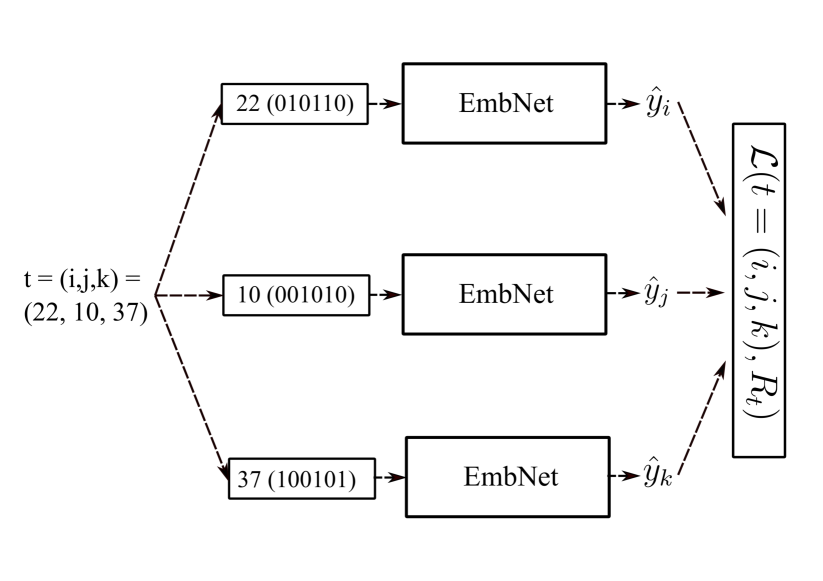
Architecture and loss. Figure 1 shows a sketch of the network architecture which is inspired from Wang et al. (2014); Schroff et al. (2015); Cheng et al. (2016); Hoffer and Ailon (2015). The central sub-module of the architecture is what we refer to as the embedding network (EmbNet), which is a three layer, fully connected neural network with Rectified linear unit (ReLU) activation functions. One such network takes a certain encoding of a single data point as input and outputs a -dimensional representation of data point . The EmbNet is replicated three times with shared parameters. The overall OENN network now takes the indices corresponding to a triplet as an input. It routes each of the indices to one of the copies of the EmbNet, which then return the -dimensional representations , respectively (cf. Figure 1). The three sub-modules are trained jointly using the triplet hinge loss, as described by the following objective function:
On the choice of parameters. We run an extensive set of simulations to find good rules of thumb to determine the parameters of the network architecture and the input encoding. We provide the results of these simulations in the supplementary (see Section J).
Difference to previous contrastive learning approaches. As described earlier, our architecture is inspired by Wang et al. (2014); Hoffer and Ailon (2015). However, note that we have no access to representations for the input items and our network takes completely arbitrary representations for the input items. Additionally, in this line of work, triplets are typically contrastive, which is of the form which indicates that and belong to the same class and is sampled from a different class. In contrast, we randomly sample triplets from the set of items.
3 EXPERIMENTS AND FINDINGS
In this section, we provide the first thorough and comprehensive evaluation of all the OE algorithms presented in Section 2. To perform this evaluation, we implemented 10 different algorithms (including OENN) with both CPU and GPU support.111Private, anonymous link to the code:https://rb.gy/kuofed. Code will be made public on github after publication. We conducted around 500 experiments using 15 different datasets and evaluated them using 5 different evaluation criteria.
3.1 Experimental Setup
Triplet Generation. Given a ground-truth dataset, we generate triplets based on the Euclidean distances of the data. To generate a triplet, we sample the indices of 3 items uniformly from the dataset and evaluate whether or vice versa. Accordingly, either the triplet or is added to the training set. For each dataset and experiment, unless specified otherwise, we generate triplets based on Euclidean distances, where refers to the dimension of the embedding space for some . We refer to as the triplet multiplier. This is a known theoretical lower bound on the number of active triplets required to reconstruct the original embedding up to similarity transformations (Jain et al., 2016). In addition, our extensive empirical investigation also reveals that passively generated triplets also suffice to achieve good reconstructions of the original embedding (for instance, see the experiments on increasing number of triplets in Section 3.4). Therefore, unless specified otherwise, we simply set . Active algorithms have access to an oracle which can provide any queried triplet.
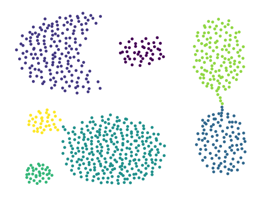
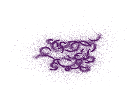
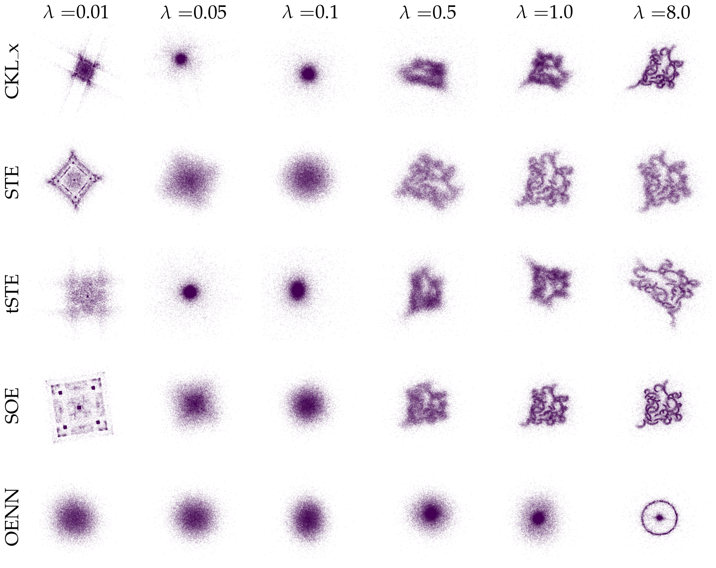
Datasets. We use a variety of datasets to generate training triplets for the ordinal embedding task. The datasets range from a few hundred items to millions of items and from 2 dimensions to 784 dimensions. To enable better visual evaluation of the embeddings generated by the various algorithms, we consider a variety of 2D datasets from Fränti and Sieranoja (2018). For a thorough evaluation, we also consider a range of high-dimensional real (CHAR (Dua and Graff, 2017), USPS (Hull, 1994), MNIST (Lecun and Cortes, 1998), Fashion MNIST (Xiao et al., 2017), KMNIST (Clanuwat et al., 2018), Forest Covertype (Dua and Graff, 2017)) and synthetic datasets (Uniform, Mixture of Gaussians). In the supplementary (A) we summarize the properties of the datasets in detail and describe in which experiment each of the datasets is used.
Algorithms and Implementation. Our library consists of all nine OE methods summarized in Table 1 and the new OENN method. We implement all algorithms in Python 3.7 using the PyTorch library (Paszke et al., 2019), which allows us to use GPU resources for training. We describe our hardware settings in the supplementary (Section B). We optimize all methods with a stochastic gradient descent using adaptive learning rates (ADAM Kingma and Ba (2014)), with the exception of FORTE, which uses a line-search based on the implementation by Jain et al. (2016). The parameter selection for each method is described in the supplementary (Section B).
Evaluation. In our experiments, we use the following criteria to evaluate the embeddings obtained by the algorithms.
-
1.
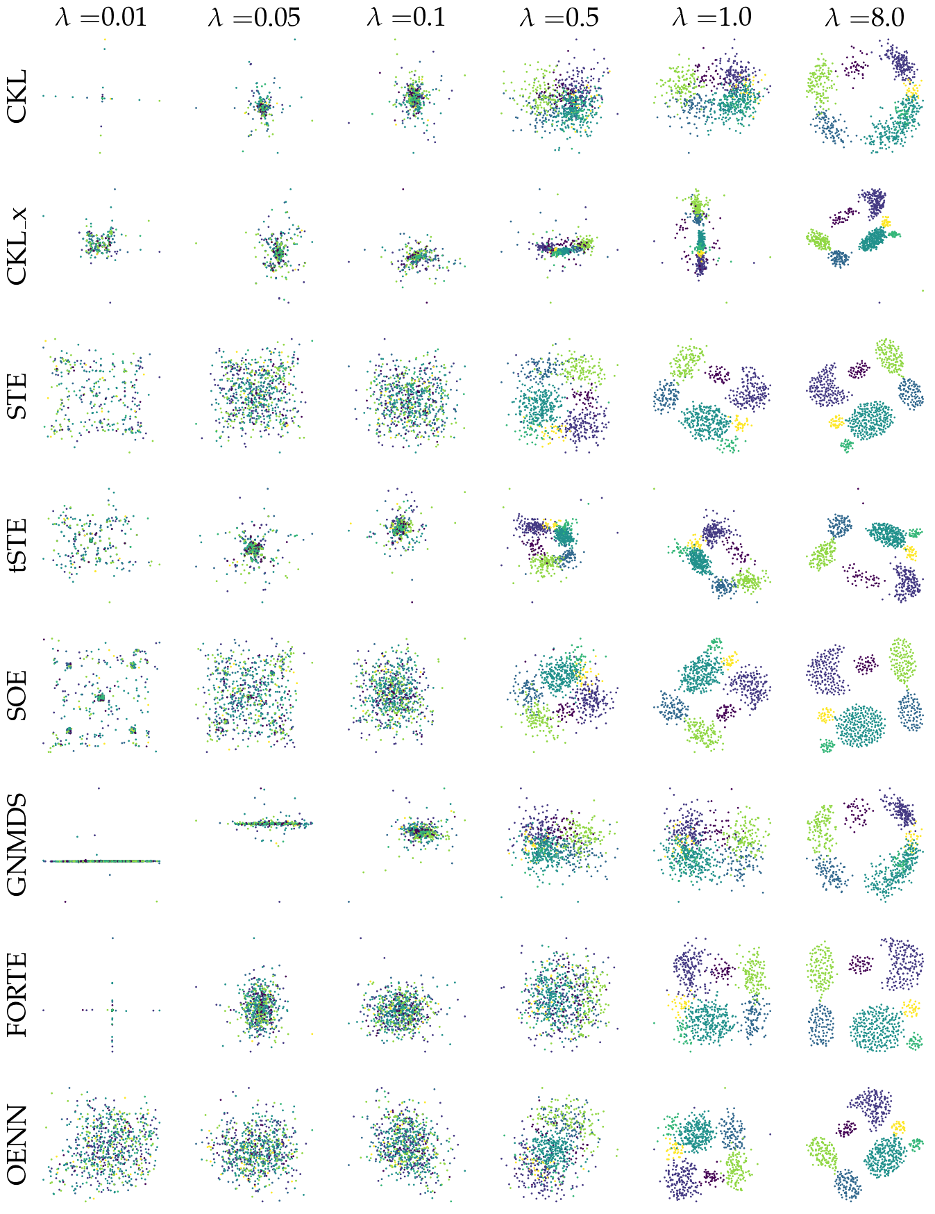
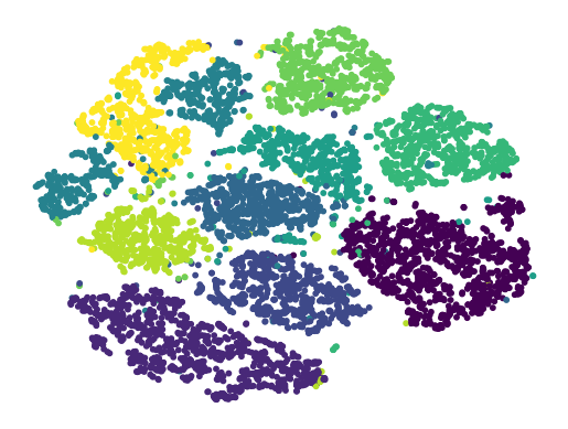
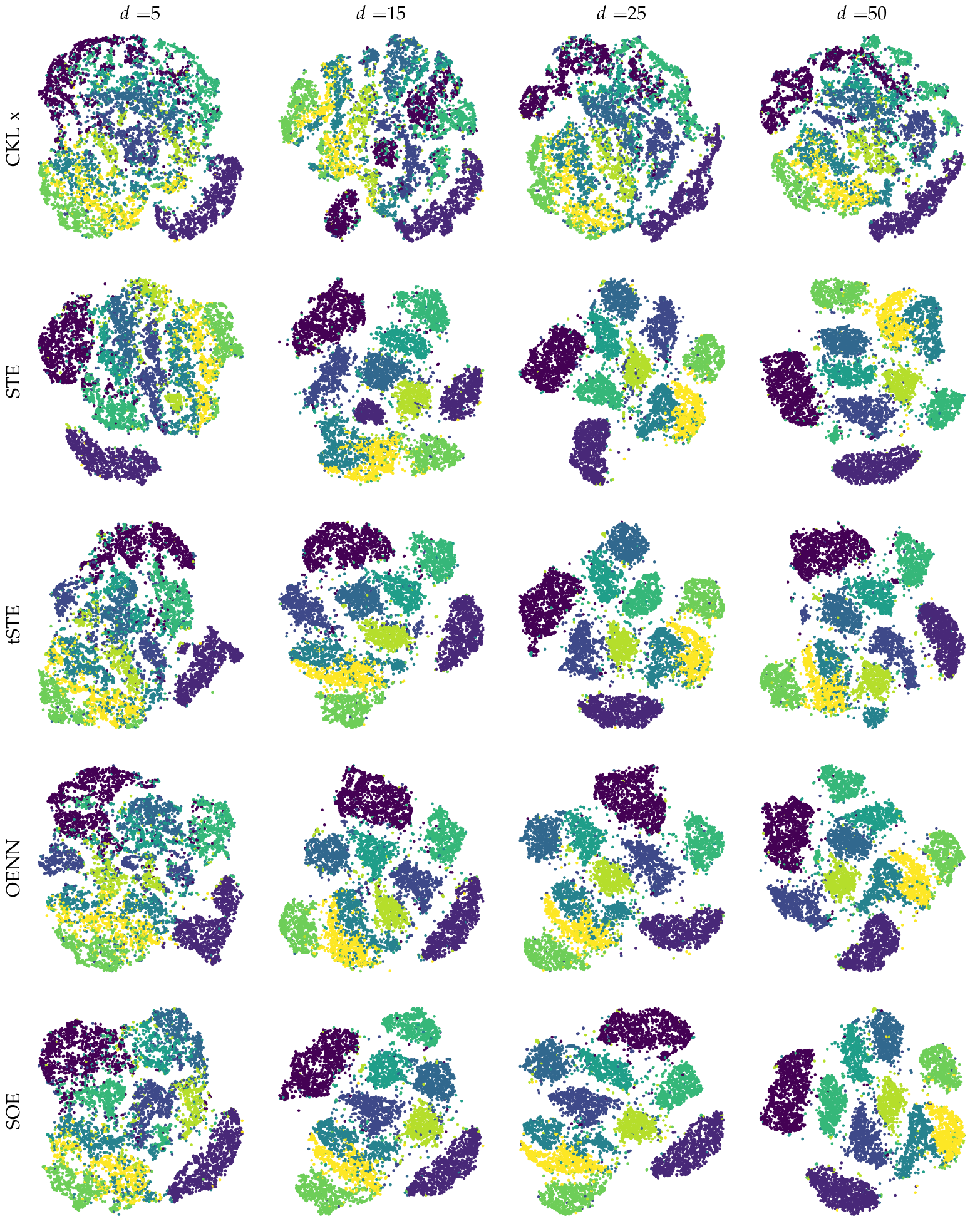
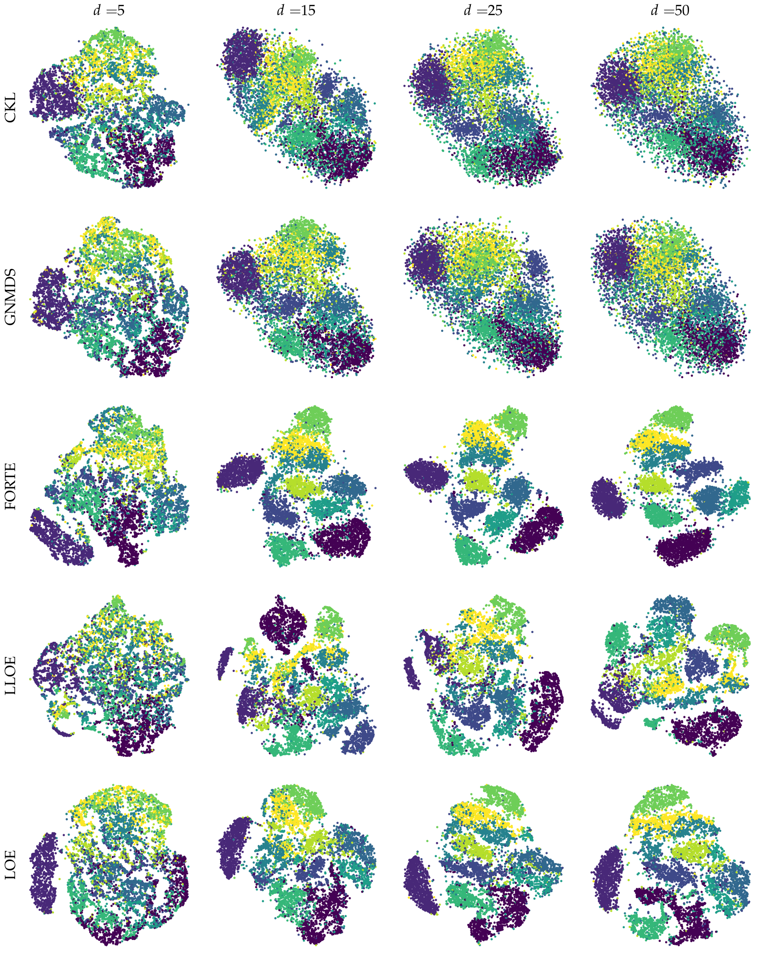
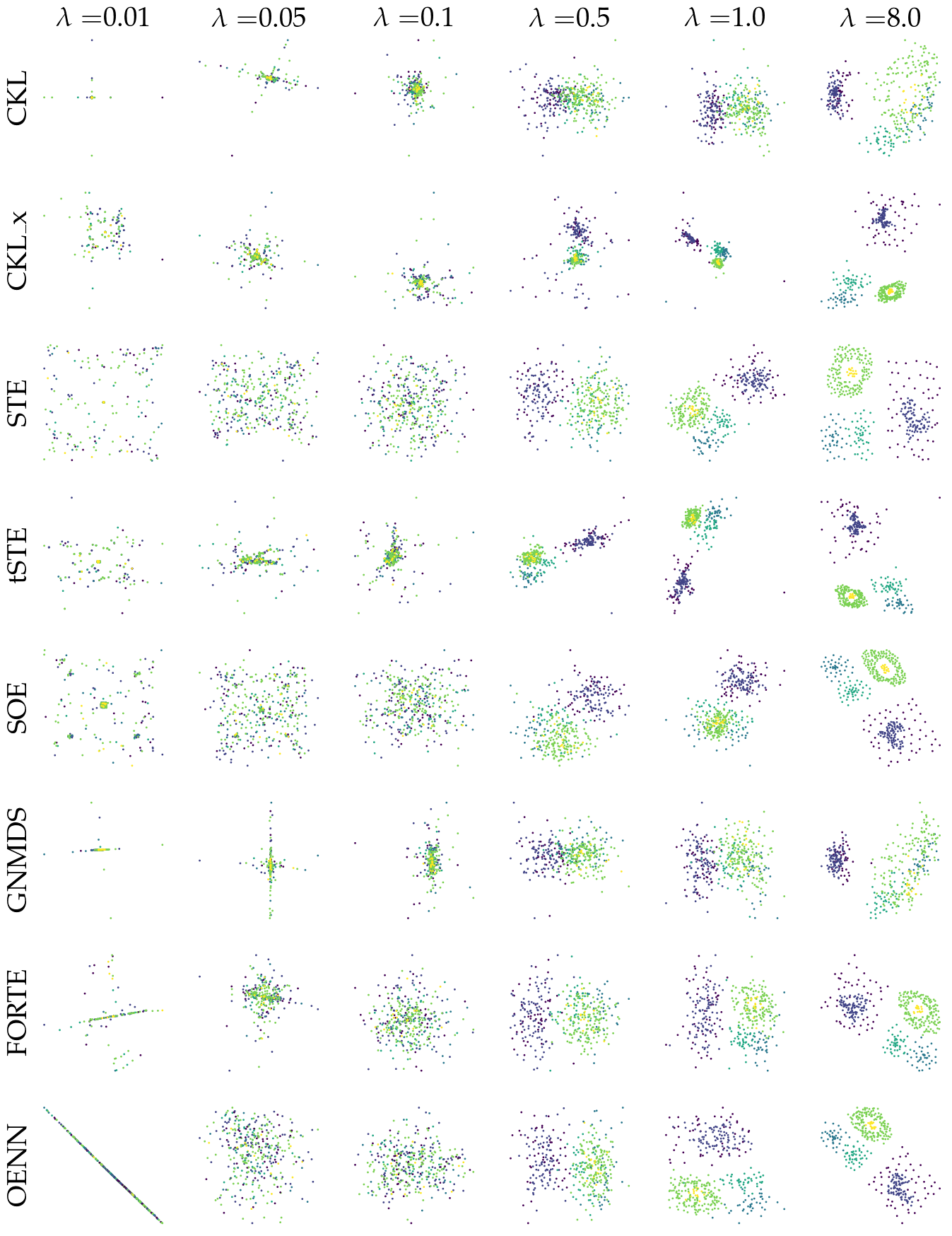
Qualitative Assessment. In the case of two-dimensional embeddings, we simply plot the embedding output. In case of higher dimensional embeddings, we visualize the high-dimensional embedding in two dimensions using t-SNE (van der Maaten and Hinton, 2008). Previous work in OE also report visualisation as an evaluation criteria (Agarwal et al., 2007; Tamuz et al., 2011; van der Maaten and Weinberger, 2012).
-
2.
Triplet Error. Train triplet error is the proportion of the input triplets that are not satisfied by the estimated embedding. To evaluate the test triplet error, we randomly sample triplets, independent of the set of training triplets, based on the ground-truth data. This metric measures generalization of the obtained embedding to held-out triplets.
-
3.
Procrustes Disparity. Measures the distance between an orthogonal transformation of the output embedding and the ground-truth (Gower et al., 2004). We minimize the Frobenius norm between the original embedding and an orthogonal transformation of the embedding output : . If the ordinal embedding has a lower dimension, we consider the embedding in the original dimension by adding zero columns to . Note that this metric can only be utilized when a ground truth embedding is available which is indeed the case for all of our datasets.
-
4.
kNN Classification Error. In order to capture how well the local structure is preserved, we train a -nearest neighbour classifier on 70% of the dataset and measure the error of the remaining 30% of the data. We fix the parameter . Therefore, we can only report the performance of the algorithms via this evaluation metric on labelled datasets.
-
5.
Running Time. The running time is measured as long as the change in train triplet error on a randomly chosen subset of training triplets is at least .
3.2 For a General Ordinal Embedding Task, which Algorithm should you use?
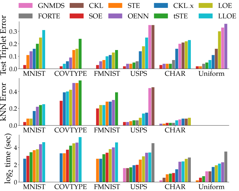
We first investigate the general performance of the algorithms on six different datasets with a wide range of sample sizes ( to ) and input dimensions ( to ). We evaluate the performance of each algorithm on all datasets using our evaluation criteria. Algorithms which optimize over the Gram matrix, that is, CKL, GNMDS, and FORTE cannot be evaluated on datasets over items since the Gram matrix becomes too large to fit in the GPU and the optimization is computationally prohibitive on a CPU. Therefore, we exclude these methods in evaluations with larger datasets. We present the results of our evaluation in Figure 2 and summarize some of the key findings here.
-
•
In terms of reconstruction of the original embedding, without exception, SOE is the best performing algorithm. This can be observed in Figure 2 which shows that SOE achieves the lowest test triplet error compared to all the other methods.
-
•
SOE is also consistently among the best performing methods for preserving the local neighborhood as measured by the kNN error. Contrary to the popular belief that t-STE better preserves the local neighborhood, our experiments suggest that it can often be among the poorly performing algorithms in this respect.
-
•
Across the datasets, SOE incurs median running time, but among the algorithms which have good reconstruction performance, there is no algorithm with clear advantage in running time over the others.
-
•
Perhaps surprisingly, CKL and GNMDS have the lowest running times of all the methods: even though each gradient step scales as the number of iterations required for convergence of these methods is significantly lower than that of the other methods. However, among the passive methods, they demonstrate the worst performance which is consistent with similar observations in the literature (van der Maaten and Weinberger (2012); Ghosh et al. (2019)).
-
•
Consistently across all the experiments, algorithms that directly optimize over the embedding matrix appear to outperform those that consider optimization over the gram matrix. Among all Gram matrix based methods, only FORTE is somewhat competitive with the others with respect to triplet error and kNN error, although, the running time is significantly higher.
-
•
Active, landmark-based approaches: LOE and LLOE do not demonstrate consistent superior performance in either running time or accuracy. In particular, the running time of LLOE is consistently amongst the worst, since, unlike the other methods, LLOE cannot be fully parallelized over GPU cores.
3.3 Do the Non-Convex Approaches to OE suffer from Local Optima?
Finding a feasible solution to the OE problem constitutes optimizing over a non-convex objective function and hence some ordinal embedding algorithms use convex relaxations or majorizing functions to make the optimization problem easier to handle (Agarwal et al., 2007; Terada and von Luxburg, 2014). Other OE algorithms involve optimizing over non-convex landscapes by means of first order methods. A natural question to ask here would be “Are local optima a hindrance to these OE algorithms due to the non-convexity of their objectives?” In this section, we provide extensive empirical evidence that suggests otherwise. Moreover, we show that certain algorithms with non-convex objectives obtain globally optimal solutions to the problem.
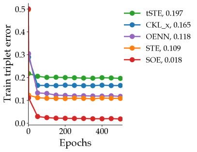
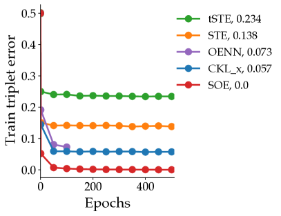
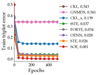
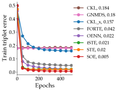
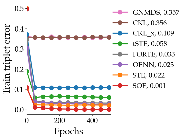
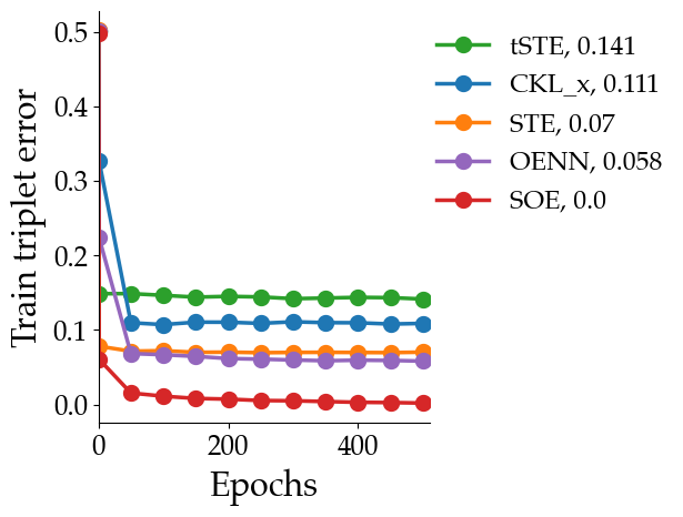
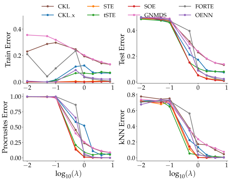
To test this hypothesis, we train all the algorithms over a selection of datasets (see Table 1 in the supplementary) and plot the train triplet error with increasing number of epochs. The main objective of this experiment is to verify whether the non-convex approaches are able to achieve near zero train triplet error which would indicate obtaining a globally optimal solution. Note that the loss functions used by different algorithms vary both in nature and in scale, therefore the train triplet error is used as a unifying metric for convergence. Train triplet error cannot be meaningfully defined for active approaches since unlike passive methods, they query specific triplets from an oracle and are not provided a set of training triplets. Therefore, we exclude them from the current experiment. Figure 3 depicts the train triplet error of eight OE methods on three datasets. The final value of the train triplet error after epochs is reported in the legend of each plot. As it is evident from plots, SOE is the only algorithm that consistently, across all the datasets, obtains the globally optimal solution, that is, attains nearly zero train triplet error. OENN, STE, and t-STE attain relatively small training error. Interestingly, even though the learning objective of OENN and SOE are near identical, we find that on MNIST, OENN indeed appears to get stuck in a local optimum while SOE does not. We infer this since the train triplet error attained by OENN plateaus after around 200 epochs and remains high thereafter. In line with the rest of our experiments, CKL and the convex approach GNMDS attain high train triplet error. To conclude, most of the non-convex approaches to OE do not seem to suffer from local optima. In particular, given sufficiently many epochs and with an appropriate learning rate, the optimization of SOE always finds a globally optimal solution. Additional results from this experiment are provided in the Supplementary (Section D)
3.4 Which Algorithms perform Better in Different Triplet Regimes?
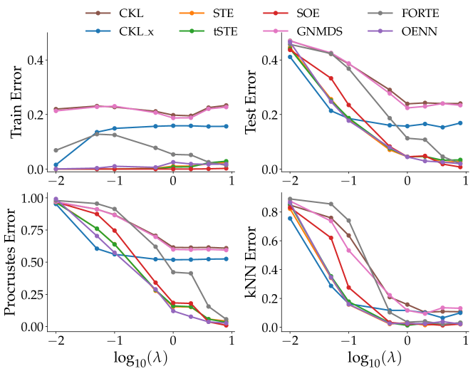
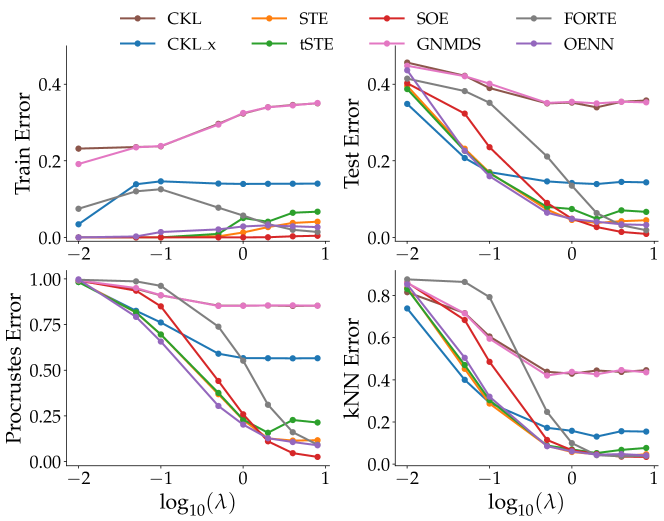
In this experiment, we vary the number of triplets as a factor of and examine the performance of all methods. Since the number of available triplets cannot be fully controlled for the active approaches, namely, LOE and LLOE, we exclude them in our analysis. In this experiment, we vary the number of triplets with the triplet multiplier ranging from to for three high-dimensional datasets and seven 2D datasets. We primarily focus on two aspects of the obtained embeddings: How well does the obtained embedding reconstruct the original embedding, as measured by the Procrustes and test triplet errors and how well does it preserve the local neighborhoods which is quantified using kNN error.
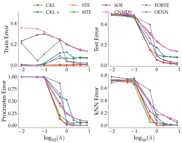
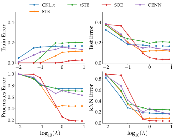
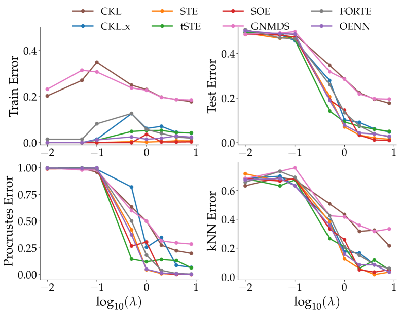
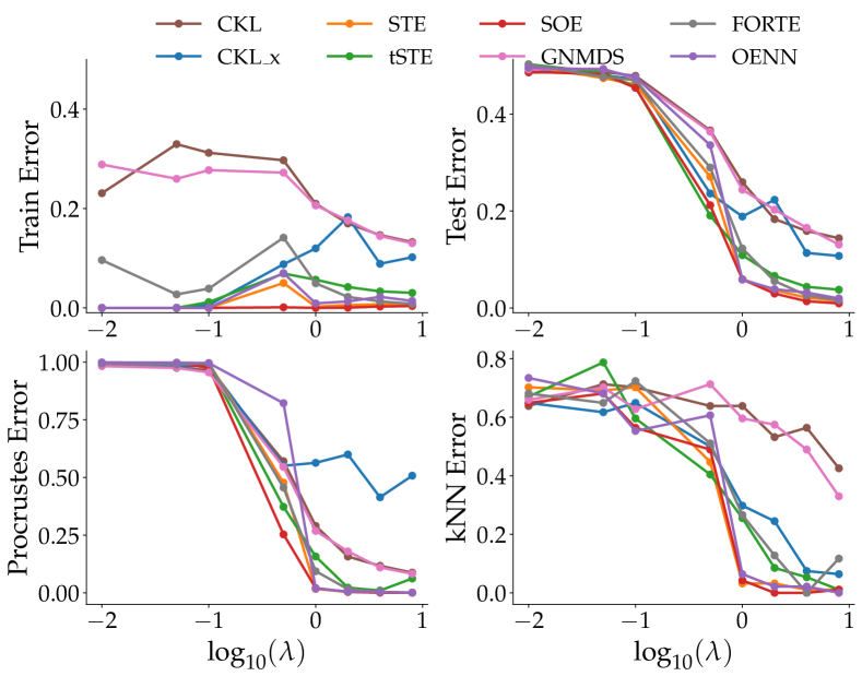
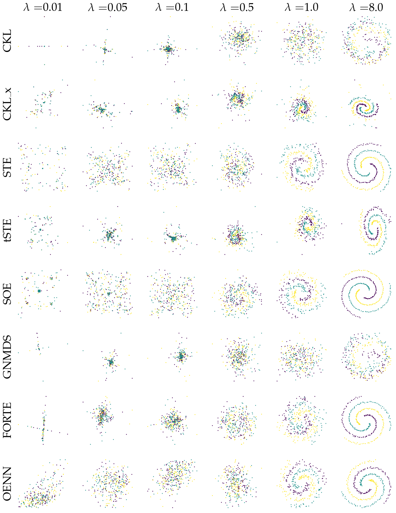
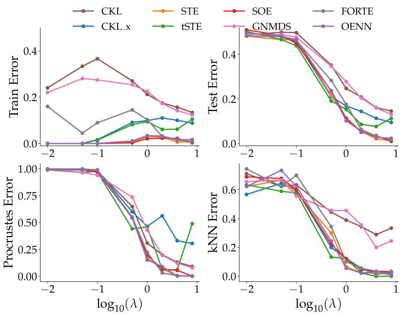
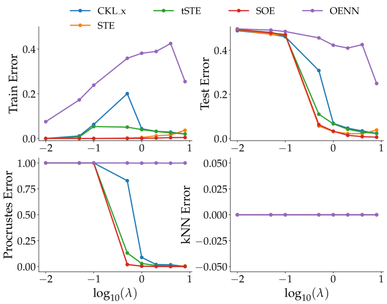
We observe two different regimes in the parameter space of the triplet multiplier : the low triplet regime where the number of available triplets are less than and the large triplet regime, where the number of triplets are larger than We make this distinction following our observation in our experiments that there is a relatively sharp transition in the Procrustes error (or test error) when the number of available triplets is between to This can, for instance, be clearly observed in Figure 4.
Small Triplet Regime.
Intuitively speaking, when the number of available triplets is small it should be easier to produce an embedding that does not violate triplet constraints. On the other hand, a small set of triplets does not uniquely specify an embedding up to similarity transformations. Therefore, without additional constraints, the Procrustes error or the test triplet error which indicate the quality of reconstruction of the original embedding can be rather high. This is reflected for in Figure 4, where we plot the Procrustes error and kNN error on two different datasets for all the embedding methods.
For most datasets, when the number of triplets are less than , none of the algorithms achieve better reconstruction error than a randomly initialized embedding, that is a Procrustes error of (see, for example, Figure 4).
Large Triplet Regime.
When the number of triplet constraints are large enough, embeddings that can satisfy all the constraints are unique up to similarity transformations (Kleindessner and von Luxburg, 2014; Jain et al., 2016). Therefore, the train triplet error often faithfully reflects the test and the Procrustes error in this regime. Since SOE always achieves the best train triplet error, as expected, in the large triplet regime it is also the best performing method in terms of reconstructing the original embedding as well as in preserving the local neighborhood (see Figure 4) . Some of the other OE approaches, namely STE, OENN, and FORTE achieve good generalization in this regime for a majority of the datasets. However, unlike SOE, on a small fraction of the datasets, they fail to achieve good training as well as test errors providing more evidence supporting the hypothesis that SOE does not suffer from local optima unlike the other non-convex approaches.
Other findings.
-
•
Preliminary evaluation in van der Maaten and Weinberger (2012), which compared t-STE with STE, seemed to suggest that t-STE better preserves the local neighborhood. Our extensive evaluation finds some evidence to the contrary. For seven out of the ten datasets, in both the small and the large triplet regimes, STE outperforms t-STE on both Procrustes error as well as on kNN classification error.
-
•
In the large-triplet regimes, across most of the datasets, the worst performing methods are CKL and GNMDS. This trend can be observed in other experiments as well: Gram matrix approaches are the worst performing methods with the exception of FORTE.

3.5 Which Algorithms perform Better for Low Embedding Dimensions?
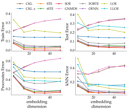
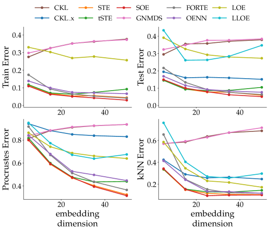
In this experiment, we evaluate the performance of the embedding algorithms by varying the embedding dimension. The number of triplets used are kept constant at . A low embedding dimension is a hard constraint on the OE problem since we reduce the degrees of freedom to fulfill all triplet constraints. On the other hand, with higher embedding dimensions it is easier to find an embedding that satisfies a larger number of triplet constraints. Here, since the embedding dimension is always chosen to be smaller than the input dimension, we expect the train error, as well as reconstruction errors, to decrease as the embedding dimension increases. Further, it would be of interest to see if some algorithms perform better than the others in the low dimensional setting in terms of either reconstruction or in preserving the local neighborhood. In Figure 7, we observe that most methods obtain lower Procrustes and kNN error with higher embedding dimension. SOE, STE, tSTE, and OENN exploit the higher dimensions the most as evidenced by the relatively sharp decrease in both kNN and Procrustes errors. Interestingly, CKL and GNMDS, which optimize over the Gram matrix and, hence, do not require the dimension as a parameter, worsen in performance with increasing embedding dimension. In this experiment, we do not observe a favourable inductive bias for any algorithm when the embedding dimension is small.

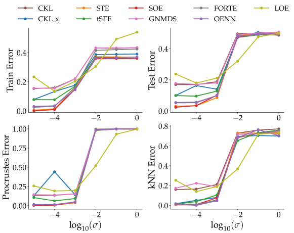
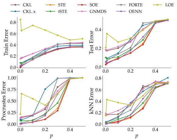
3.6 What is the effect of noise on the performance of OE algorithms?
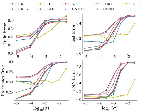
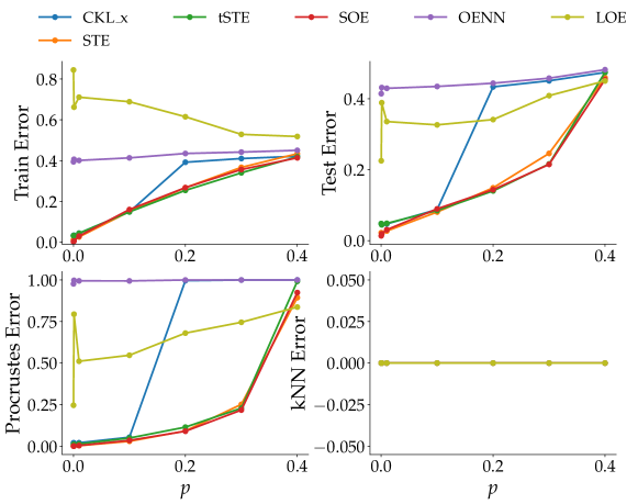
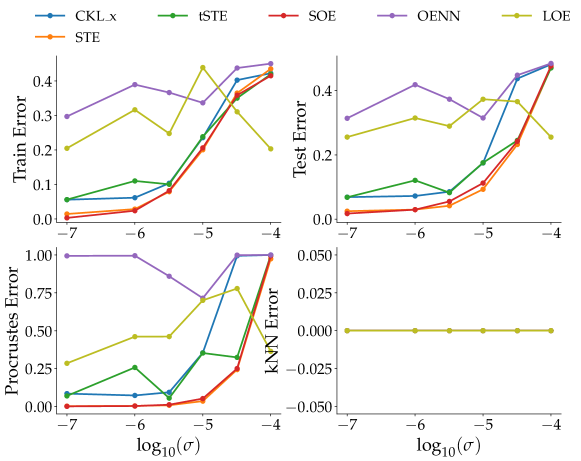
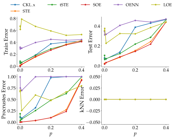
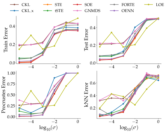
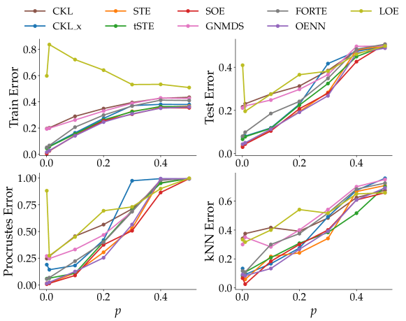
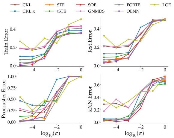
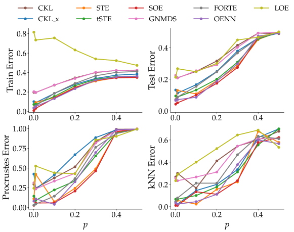
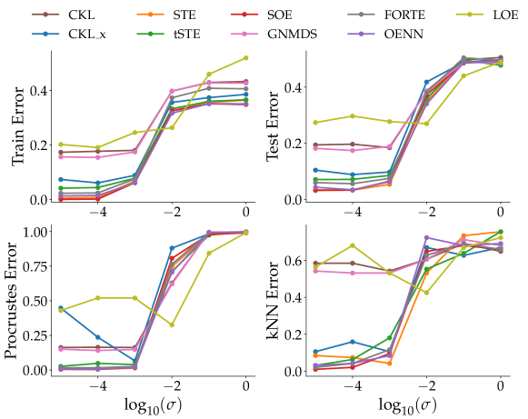
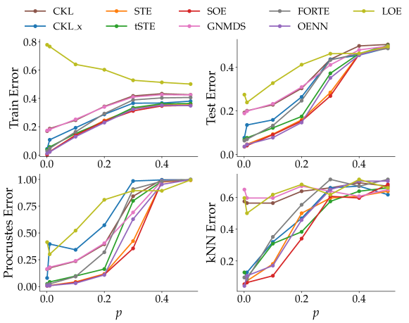
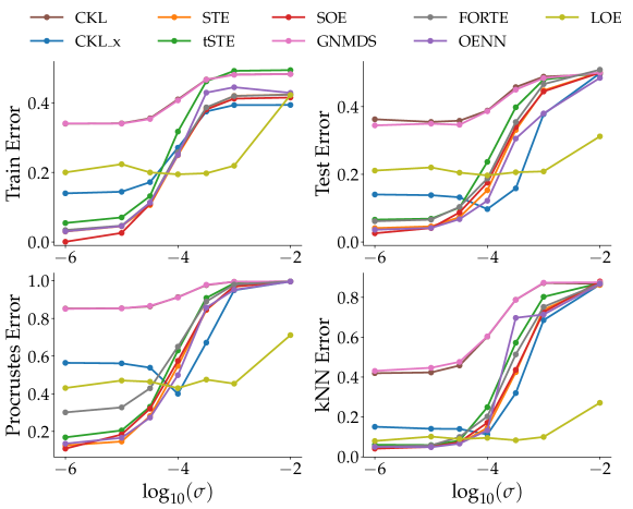
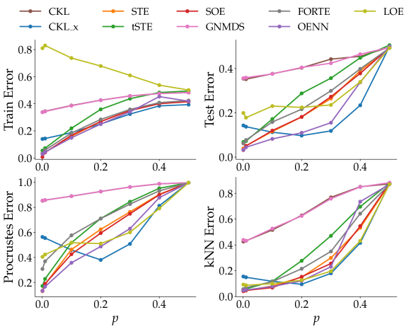
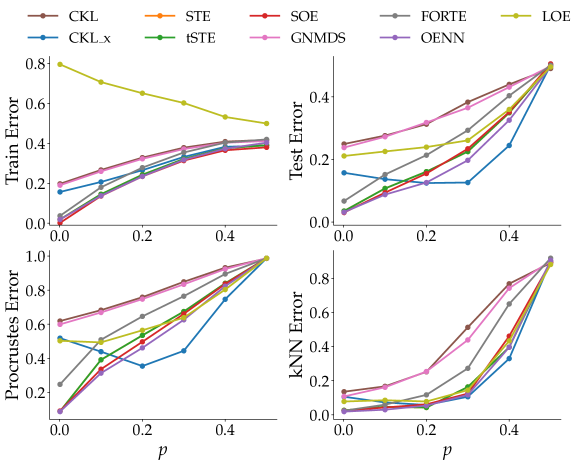
Here, we evaluate the effect of noise on the performance of OE algorithms. To this end, we consider two noise models on our training triplets.
Bernoulli Noise Model.
In this model, we independently flip a true triplet to with probability . This model is fairly intuitive and the probability naturally determines the level of noise.
Gaussian Noise Model.
When creating triplets from the ground truth, we need to evaluate two distances: and . In this noise model, we independently add a centered Gaussian to the distances. We then generate triplets by comparing the noisy distances. The variance represents the noise level.
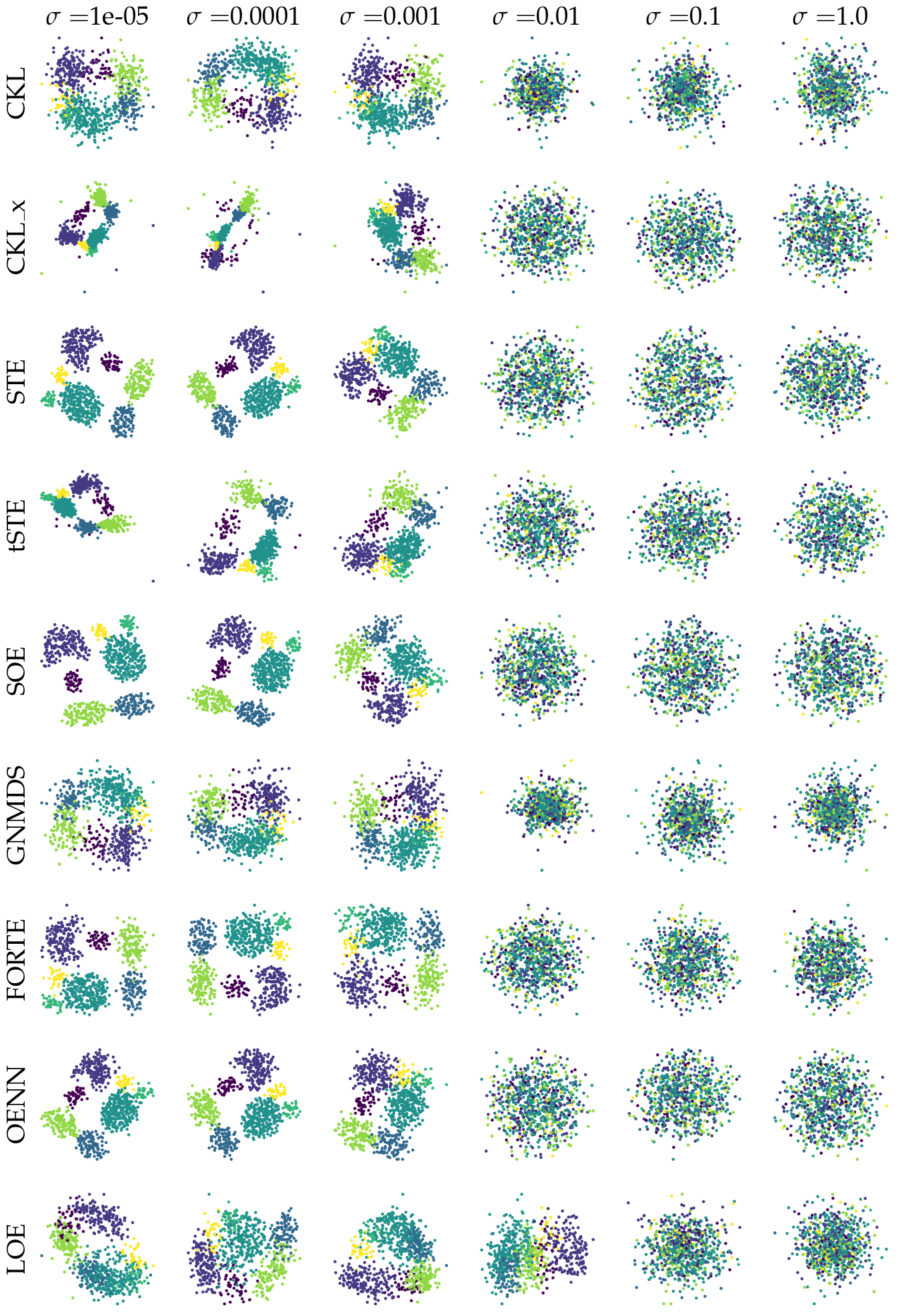
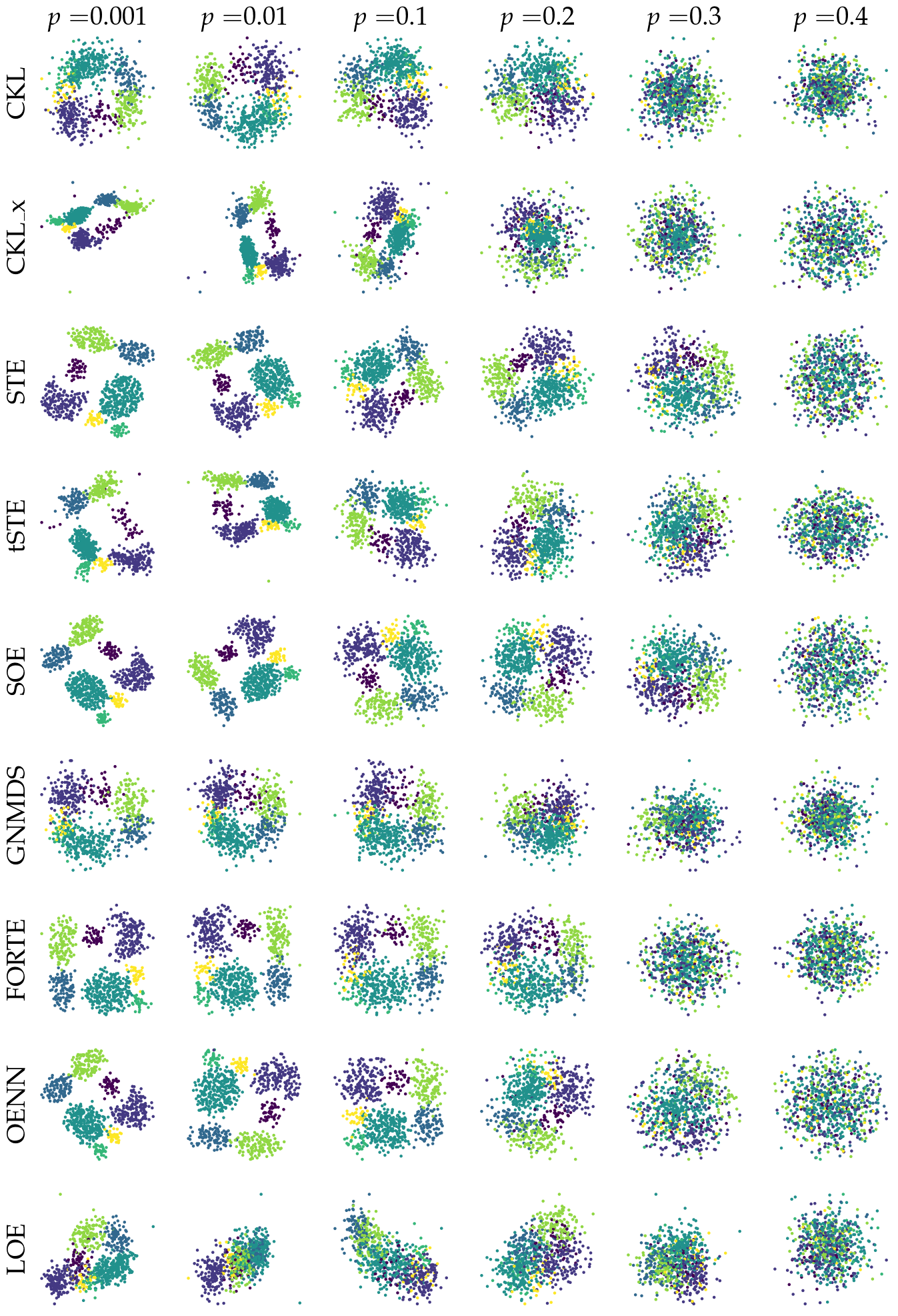
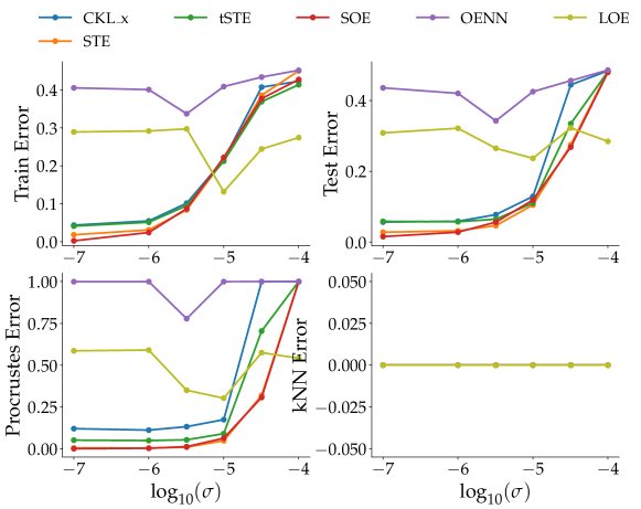
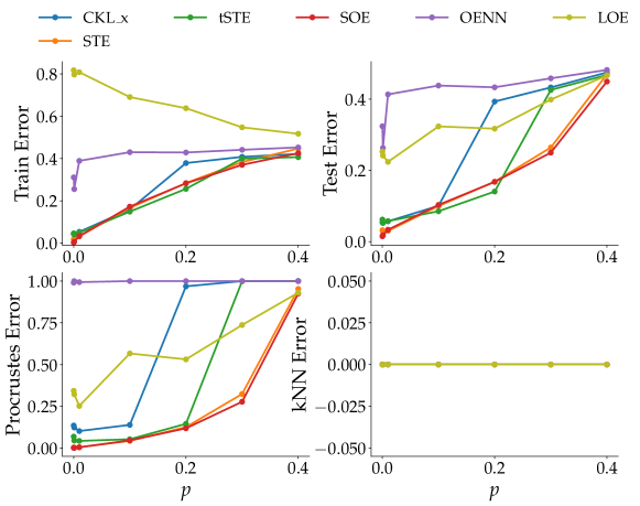
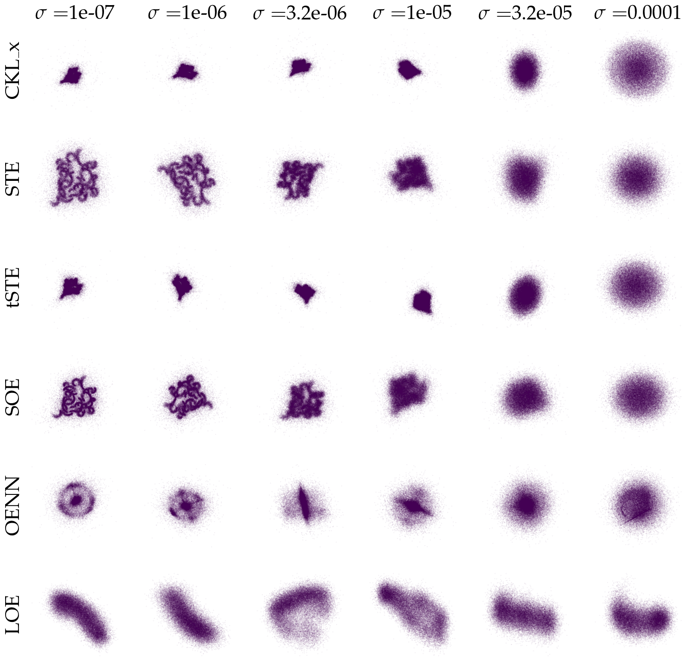
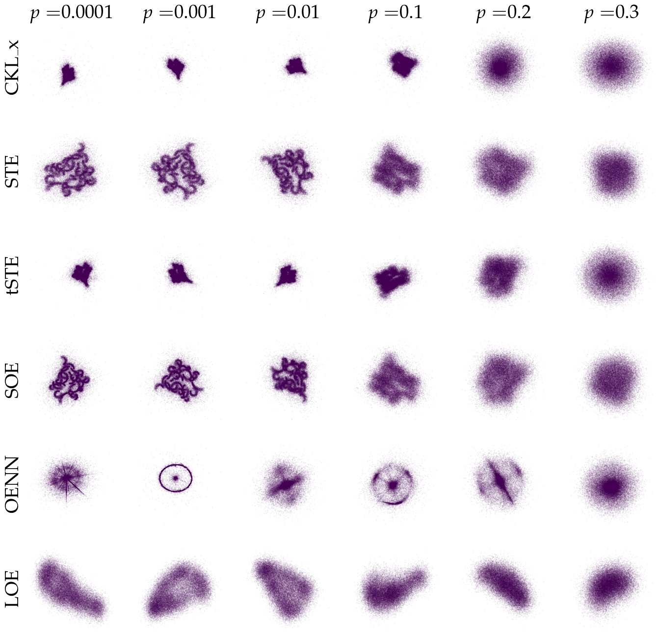
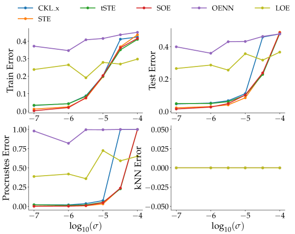
To conduct the experiment, we vary the noise level and evaluate the performance of the algorithms for each of the noise models. The number of triplets used are kept constant at The performance of all the OE methods naturally deteriorates with increasing noise levels under both noise models (see Figure 10). Consistent with the other experiments, under low levels of noise, SOE clearly matches or outperforms the rest of the algorithms. Under moderate to high levels of noise, all the simple distance-based methods: SOE, STE, t-STE, and CKLx perform similarly and in line with the rest of the experiments, they outperform the gram-matrix based approaches as well as the more elaborate neural network or landmark-based approaches.
3.7 Which Methods scale Better with Sample Size and Input Dimension?
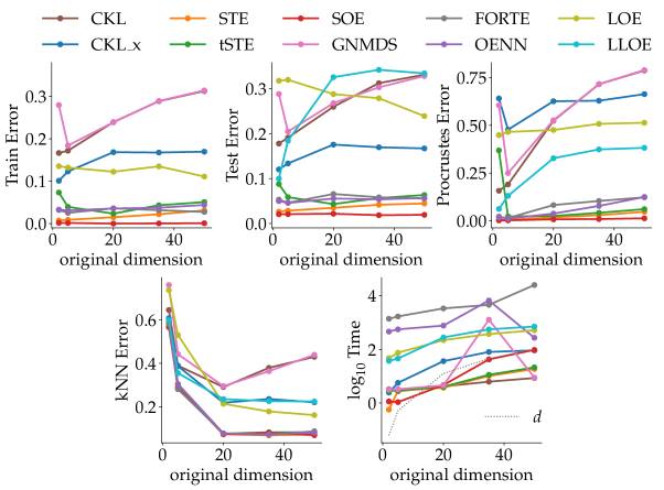
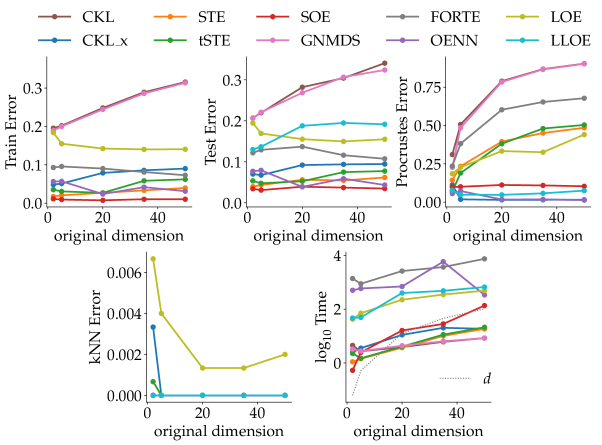
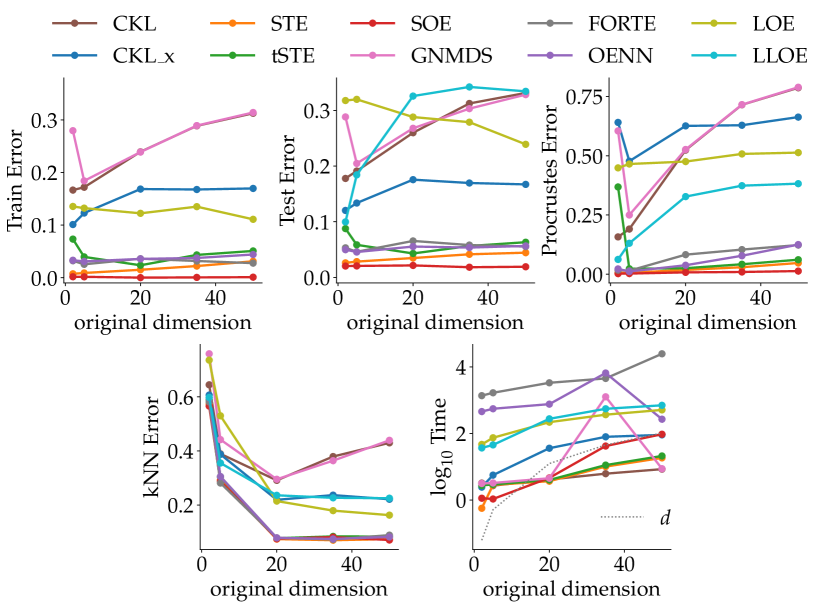
In this experiment, we investigate the running time of the algorithms with varying input dimension and with varying sample size. Recall that the running time of each gradient update scales as and as for algorithms optimizing over the Gram matrix and the data matrix respectively. To create datasets with increasing original dimension, we consider two different datasets: Gaussian mixture models (GMM) and PCA MNIST. To generate data from GMM, we sample from Gaussian mixtures in increasing input dimension. For PCA MNIST, we project the original MNIST data using PCA into Euclidean space with increasing dimensions. We keep the embedding dimension for ordinal embedding the same as the dimension of the generated datasets.
Increasing Input Dimension d.
As expected, the running time of all methods increases with input dimension. As anticipated, Figure 11a shows that running time of SOE, STE, t-STE and CKLx, which are methods optimizing over the data matrix, roughly scales as while methods optimizing over the Gram matrix roughly scale as . The running time of FORTE, OENN, and LLOE is much higher than that of the simple, non-convex approaches: SOE, STE, and t-STE. The increasing input dimension also has an impact on the methods’ performance. Only SOE consistently achieves a low procrustes error, while the procrustes error of STE, tSTE, and OENN decreases slightly.
Increasing Sample Size n.
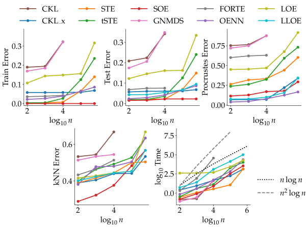
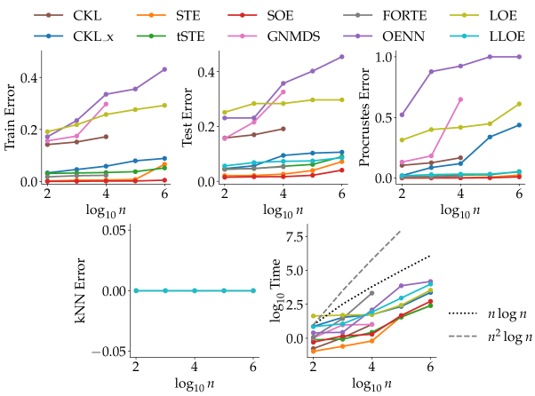
As discussed earlier, we cannot evaluate the Gram matrix approaches on datasets with more than items and therefore, we clip the sample size at this limit for these approaches. Again, as expected, algorithms optimizing over the data matrix and Gram matrix exhibit a growth rate of and respectively. OENN and LOE are an order of magnitude slower than the rest although the test error of OENN is considerably lower than that of LOE. We can observe in Figure 12 that SOE has nearly constant test error with increasing number of points while the other methods worsen in performance. STE and t-STE, which are generally well performing methods, also seem to show a sharp increase in test error with increasing sample size.
3.8 How do Methods scale on CPU vs GPU?
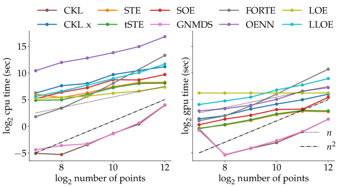
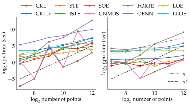
We compare the running time of various OE algorithms on CPU versus GPU with increasing sample size. We choose small sample sizes in this experiment to avoid prohibitive CPU computational cost. Figure 13 left and right respectively show the CPU and GPU times of embedding methods for the MNIST dataset. In the log-log plots shown in Figure 13, note that the slope of the line determines the growth rate of the running time with increasing . Consistent with theoretical complexity, running time of approaches that optimize over the data matrix and Gram matrix have linear and quadratic growth rate in respectively. GNMDS and CKL do have low running times since the number of iterations required for convergence to a solution are typically low, which can also be seen in our convergence experiment (see Figure 3).
The running time of all methods drops drastically on GPUs and it is clear that OE methods can utilize parallel computation in their optimization procedure. Landmark-based approaches, namely LOE and LLOE claim to have better running times, but in our experiments on both GPU and CPU we do not find sufficient evidence to substantiate this claim. LOE appears to have nearly constant running time on GPU. However, this is an artifact of the small sample size used for this experiment to allow of reasonable CPU computation time. This can be observed in our experiment (Section 3.7) which investigates the running time of methods with increasing sample size.
4 DISCUSSION
We start off by summarizing our key findings as rules of thumb for OE practitioners. In the low noise regime, the clear method of choice given sufficiently many triplets is SOE since it scales comparably in time to other well performing methods and consistently demonstrates superior reconstruction performance. For small number of points and dimensions, you can use any of these non-convex approaches: SOE, STE, T-STE, and OENN. If computational efficiency is a high priority, then on both CPU as well as GPU, unless one can considerably compromise on the quality, SOE, STE, and t-STE are the best candidates. Given sufficiently many triplets, for good reconstruction and for preserving the local neighborhood, SOE is again the top choice. In the large-sample regime or in the high-dimensional regime, SOE is a particularly good choice of OE algorithms since it appears to attain nearly constant test error with increasing sample sizes and dimensions.
When the number of triplets are sufficiently large, it has been theoretically established that the original data can be exactly reconstructed up to similarity transformations Kleindessner and von Luxburg (2014); Jain et al. (2016). Therefore, with sufficiently many triplets, an algorithm that can achieve near zero train triplet error would also obtain low reconstruction errors. Bower et al. (2018) conjectures that the optimization of the hinge triplet loss may not suffer from local optima and that every local optima is also a global optima. The optimization objective used in SOE (Terada and von Luxburg, 2014) is closely related to the hinge triplet loss and we conjecture that this might indeed hold for the optimization objective of SOE as well. Our experiments provide an abundance of empirical evidence to support this hypothesis. Interestingly, even though OENN uses the hinge triplet loss suggested by Bower et al. (2018), unlike SOE, OENN occasionally appears to suffer from local optima. Investigating this more formally could provide valuable insights into understanding non-convex optimization landscapes where local optima are also globally optimal. We leave this for future work.
Acknowledgments
This work has been supported by the German Research Foundation through the Cluster of Excellence “Machine Learning – New Perspectives for Science” (EXC 2064/1 number 390727645), the Baden-Württemberg Stiftung through the BW Eliteprogramm for Postdocs, the BMBF Tübingen AI Center (FKZ: 01IS1803 9A), and the International Max Planck Research School for Intelligent Systems (IMPRS-IS).
Appendix
In the appendix materials, we present results and details that were omitted from the main paper. In Section A, we describe the datasets and present in which experiments they were used. In Section B, we provide further details on the experimental setup. Sections C to H contain more results and findings from our experiments. In Section J, we formulate the methods and their objectives in more detail. A detailed description of our neural network approach OENN and the simulations used to choose the parameters of OENN are provided in Section J.
A DESCRIPTION OF DATASETS
The following, we describe the datasets that we use in our experiments. In Table 1, we visualize in experiments they were employed.
2D datasets.
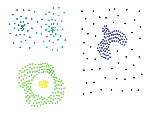
For the reconstruction of 2D datasets with ordinal embedding methods, we use various datasets collected from Fränti and Sieranoja (2018):
-
•
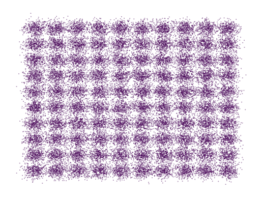
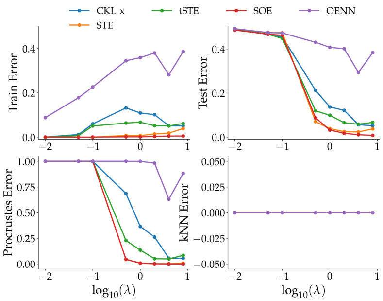
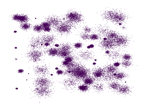
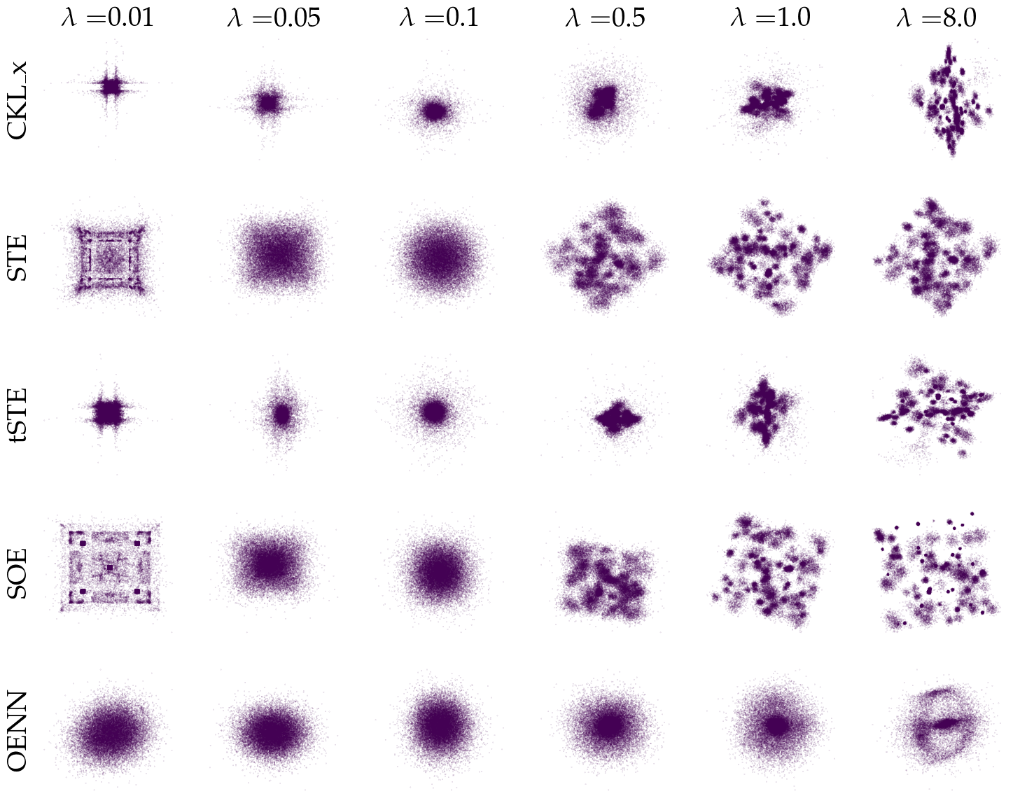
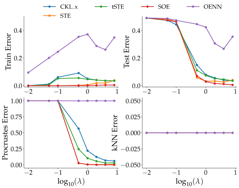
Birch1 and Birch3 (Zhang et al., 1997), with each, are artificial datasets with cluster structure: Birch1 has clusters in a regular grid, and Birch3 contains random sized clusters in random locations. However, the clusters are unlabeled.
- •
-
•
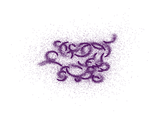
Worms (Sieranoja and Fränti, 2019) with , is a synthetic dataset containing shapes reminiscent of worms (unlabeled).
CHAR (Dua and Graff, 2017).
This dataset contains images of digits. Here, we use the test set where .
USPS (Hull, 1994).
This dataset contains handwritten images of digits. We use the train set with points.
MNIST (Lecun and Cortes, 1998).
The classic MNIST dataset contains handwritten images of digits. Again, we use the train set with .
FMNIST (Xiao et al., 2017).
The FMNIST dataset contains greyscale images of fashion items. Just as MNIST, it contains points in the train set, and consists of classes.
KMNIST (Clanuwat et al., 2018).
The Kuzushiji-MNIST train set contains images of Kuzushiji (cursive Japanese) characters. For the experiment with increasing embedding dimension, we use a random subset of points.
COVTYPE (Dua and Graff, 2017).
This dataset contains cartographic variables to predict one of forest cover types. We use the whole dataset of observations.
Gaussian Mixture, GMM.
This datasets consists of two clearly separable normal distribution with unit variance, and , where is the zero vector, and . The dimension of the dataset can be chosen.
Uniform.
For this dataset, we draw the required number of points uniformly from , where the dimension can be chosen.
| Dataset | (n, org_d, emb_d) n in 1000’s | General Exp. | Increase of triplets | Increase of points | Increase of emb_d | Increase of org_d | Convergence Exp. | CPU vs. GPU |
| 2D Data | (0.3-106, 2, 2) | |||||||
| CHAR | (1.8, 64, 30) | emb_d = 50 | ||||||
| GMM | (5, 2, 2) | |||||||
| USPS | (7.3, 256, 50) | |||||||
| MNIST | (60, 784, 50) | emb_d = 30 | ||||||
| FMNIST | (60, 784, 50) | |||||||
| KMNIST | (10, 784, 50) | |||||||
| COVTYPE | (581, 54, 30) | |||||||
| Uniform | (, 2, 2) | org_d = 10 |
B EXPERIMENTAL SETUP
B.1 Hardware.
All our experiments are conducted on one of three hardware settings. Most methods are provided with 4 CPUs and 1 GPU, while OENN requires 4 GPUs for all experiments. Due to the high number of points and the high embedding dimension, all experiments for the Covtype dataset are run on GPUs with more memory.
Hardware Setting 1 for most experiments: Intel Xeon Gold 6240 @ 2.60GHz and NVIDIA GeForce RTX 2080-Ti 11 GB.
Hardware Setting 2 for Covtype experiments: Intel Core Processors (Broadwell) @ 2GHz and NVIDIA Tesla V100 SXM2 32GB.
Hardware Setting 3 for CPUvsGPU experiments: Intel Xeon E5-2650 v4 @ 2.2 GHz and NVIDIA GTX 1080-Ti 11 GB.
For the details on the hyperparameters selected in each method, we refer to the descprition of each method in Section J.
B.2 Hyperparamters.
For all methods except OENN, we fixed the batch size to and we performed a grid search for the learning rate and other parameters on points of uniform data. We shortly summarize the results here. Due to the more complex choice of hyperparameters for OENN, we describe them in detail in Section J.3.
-
•
GNMDS. For GNMDS we use a regularization of and a learning rate of .
-
•
FORTE. The learning rate is . Similar to the implementation of Jain et al. (2016), we use the backtracking linear search parameter and the Amarijo stopping condition parameter for the line-search optimization.
-
•
CKL. For CKL we use a regularization of and a learning rate of .
-
•
SOE, STE, tSTE, and CKL_x use a learning rate of .
-
•
LOE. For LOE, the learning rate is .
-
•
LLOE. The phase one learning rate is , and the phase two learning rate is .
C GENERAL EXPERIMENTS RESULTS
| Dataset | MNIST | COVTYPE | FMNIST | USPS | CHAR | UNIFORM |
| SOE | (0.03, 0.04) 11.2min | (0.02, 0.29) 58.3min | (0.03, 0.2) 26.1min | (0.02, 0.04) 61s | (0.03, 0.03) 6s | (0.02, 0.0) 1s |
| OENN | (0.13, 0.13) 165.0min | (0.02, 0.13) 6.7h | (0.06, 0.28) 6.2h | (0.04, 0.05) 16.6min | (0.04, 0.02) 206s | (0.36, 0.0) 122s |
| STE | (0.11, 0.08) 51.3min | (0.15, 0.5) 22.5min | (0.07, 0.28) 5.2min | (0.04, 0.05) 247s | (0.04, 0.02) 4s | (0.02, 0.0) 0.6s |
| tSTE | (0.2, 0.24) 29.5min | (0.24, 0.53) 170.0min | (0.15, 0.39) 17.6min | (0.05, 0.06) 31s | (0.04, 0.03) 5s | (0.05, 0.0) 2s |
| CKL_x | (0.16, 0.17) 5.2min | (0.06, 0.39) 22.3min | (0.11, 0.28) 5.2min | (0.14, 0.15) 55s | (0.16, 0.08) 18s | (0.11, 0.0) 34s |
| LOE | (0.26, 0.08) 65.2min | (0.24, 0.51) 42.4min | (0.16, 0.29) 66.7min | (0.22, 0.12) 10.7min | (0.23, 0.07) 5.2min | (0.19, 0.0) 6s |
| LLOE | (0.31, 0.25) 7.2h | (0.04, 0.4) 27.9h | (0.1, 0.24) 6.8h | (0.25, 0.14) 27.5min | (0.23, 0.06) 153s | (0.07, 0.0) 84s |
| GNMDS | - | - | - | (0.35, 0.44) 25s | (0.2, 0.07) 0.7s | (0.33, 0.0) 10s |
| FORTE | - | - | - | (0.06, 0.06) 5.5h | (0.07, 0.03) 7.3min | (0.04, 0.0) 35.4min |
| CKL | - | - | - | (0.35, 0.45) 25s | (0.21, 0.08) 1s | (0.16, 0.0) 10s |
D CONVERGENCE EXPERIMENTS
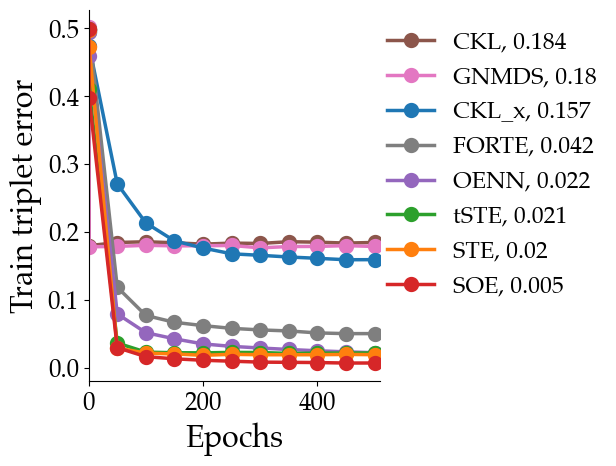
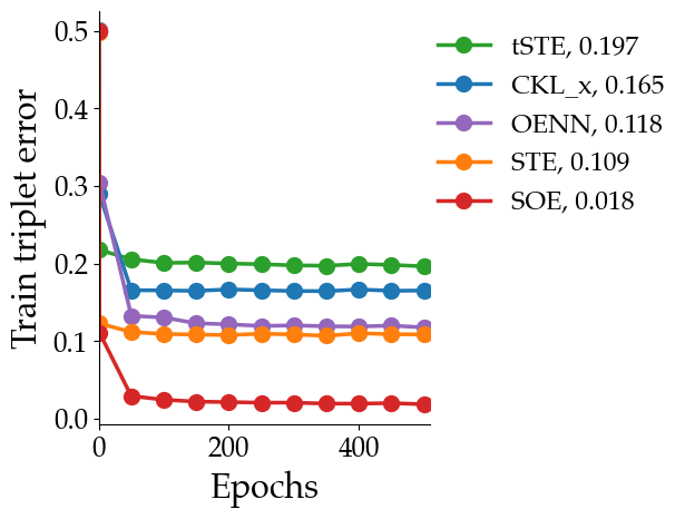
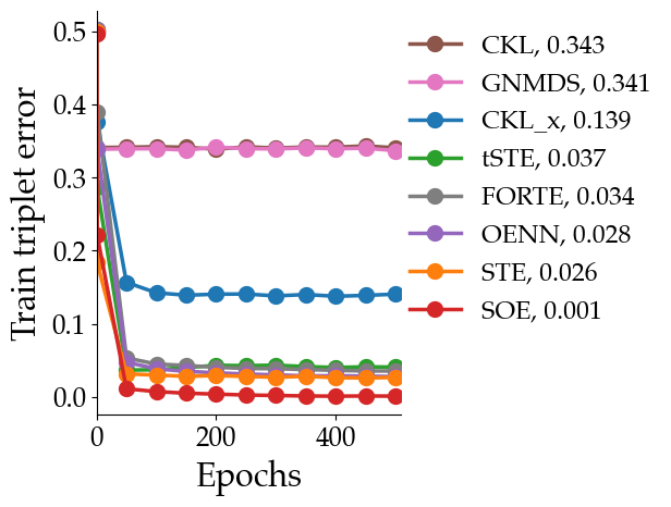
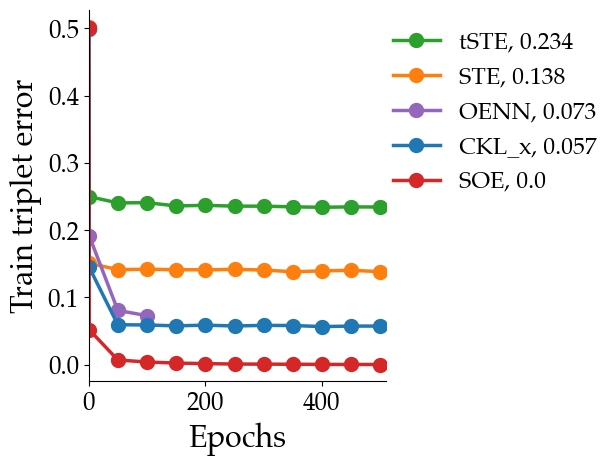
E INCREASING TRIPLETS
Other findings from this experiment.
-
•
Most algorithms demonstrate consistently poor generalization performance in the low triplet regime as measured by the Procrustes error as well as the kNN classification error even though they attain good training triplet errors. For instance, FORTE is the only gram matrix based approach that is competitive with the well-performing algorithms that optimize over the gram matrix. However, in the low triplet regime, it consistently is among the methods with the worst generalization performance even though it achieves good training triplet error.
-
•
Preliminary evaluation in van der Maaten and Weinberger (2012), which compared t-STE with STE, seemed to suggest that t-STE better preserves the local neighborhood. Our extensive evaluation finds some evidence to the contrary. For seven out of the ten datasets, in both the small and the large triplet regimes, STE outperforms t-STE on both Procrustes error as well as on kNN classification error.
-
•
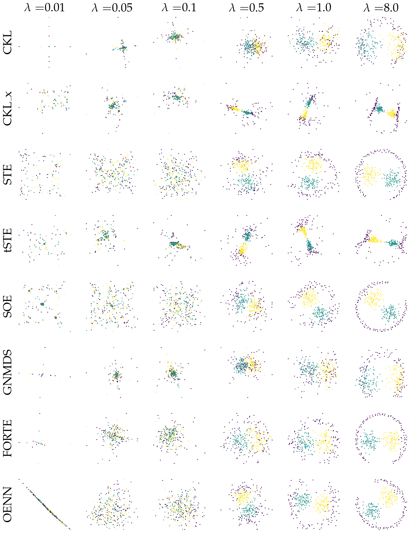
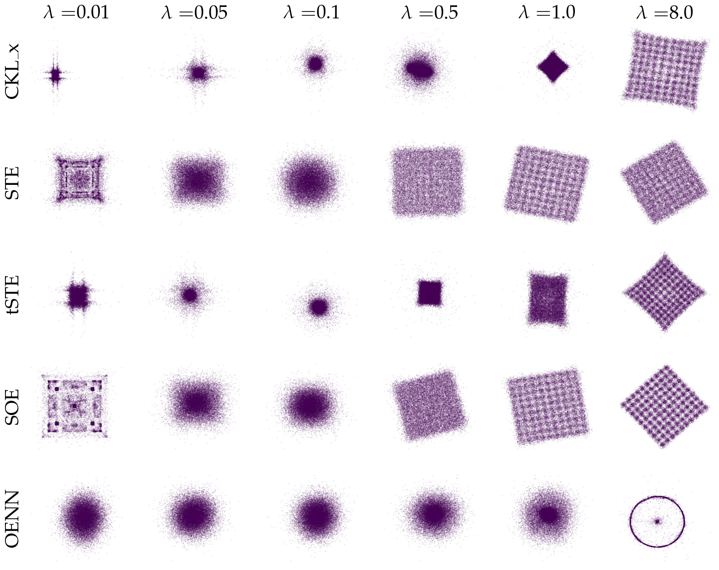
Across most of the datasets, the worst performing methods are CKL and GNMDS. This trend can be observed in other experiments as well: Gram matrix approaches are worst performing methods with the exception of FORTE. Interestingly, the variant of CKL that optimizes over the embedding directly, CKL_x, seems to be much better at preserving local neighborhoods than at reconstructing the embedding.
[.4]

Aggregation

[.4]
Compound
[.4]

Spiral
[.4]
Path-based
[.4]
Birch1
[.4]
Birch3
[.4]
Worms
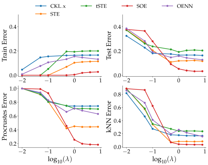
F INCREASING NOISE
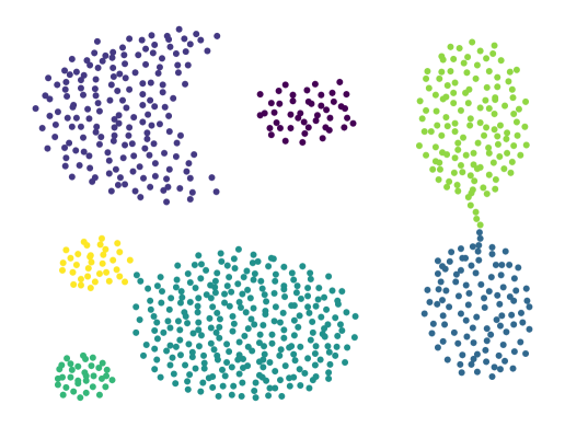
Aggregation
[.4]
Worms
[.4]

G INCREASING EMBEDDING DIMENSION

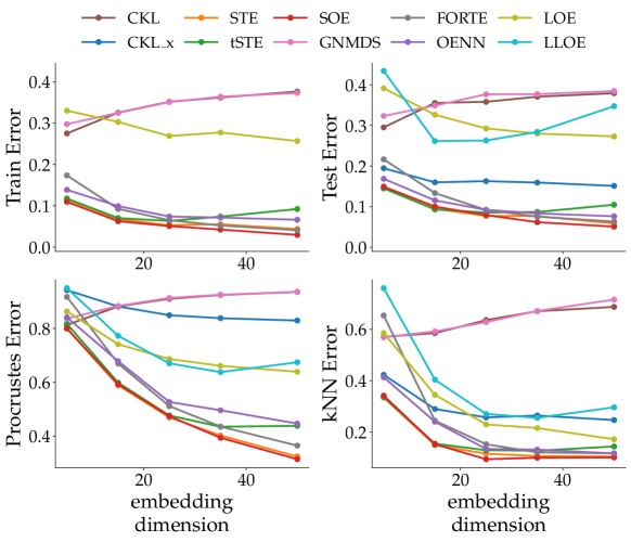
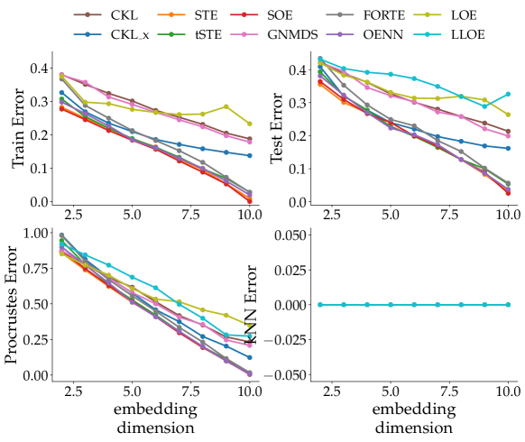
H INCREASING NUMBER OF POINTS
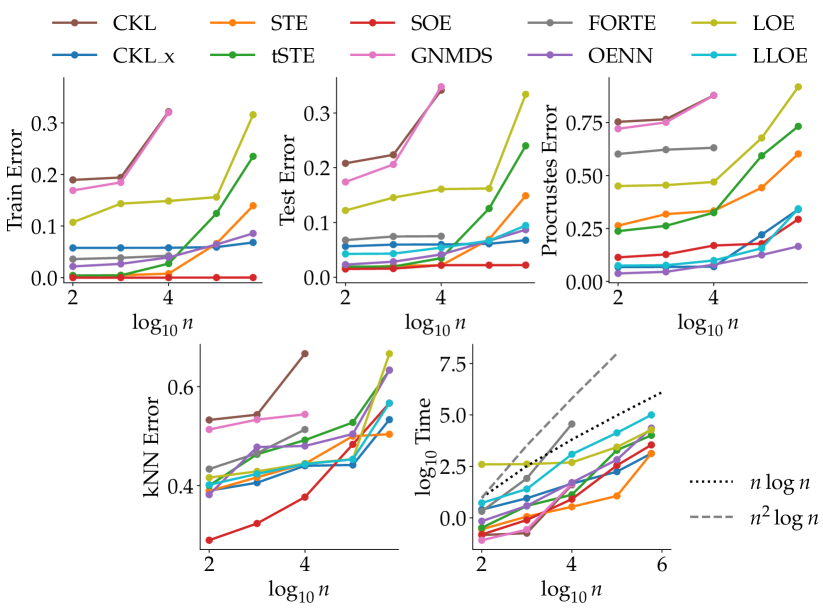

I INCREASING ORIGINAL DIMENSION
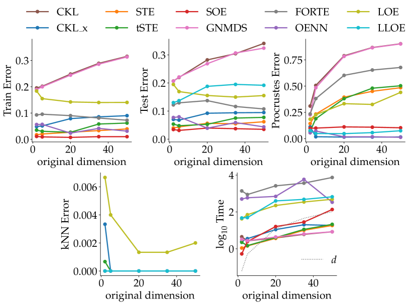
J DETAILS ON ALL METHODS
The ordinal embedding problem has first appeared in the machine learning literature as Generalized Non-metric Multi Dimensional Scaling (GNMDS) (Agarwal et al., 2007). Non-Metric Multi-Dimensional Scaling (MDS) refers to the problem of finding a Euclidean embedding, when the rank order of pairwise similarities is given (Shepard, 1962; Kruskal, 1964). The proposed method by Shepard and Kruskal is a very popular method in psychology and psychophysics. GNMDS provides a generalization to the Non-metric MDS by considering a set of quadruplet questions, instead of the full rank of distances, as the input. The quadruplet implies that the distance of to should be smaller than the distance of to . Having access to quadruplets, one can reconstruct the full rank of pairwise distances. Thus, assuming a smaller subset of quadruplet information is a generalization of the Non-Metric MDS. There have been various approaches to the problem in the last decade. However, they all share the same spirit as they optimize a loss function to ensure that triplet (or quadruplet) information are satisfied. We briefly discuss the various objective functions and their properties.
J.1 Detailed Description of the Ordinal Embedding Neural Network (OENN)

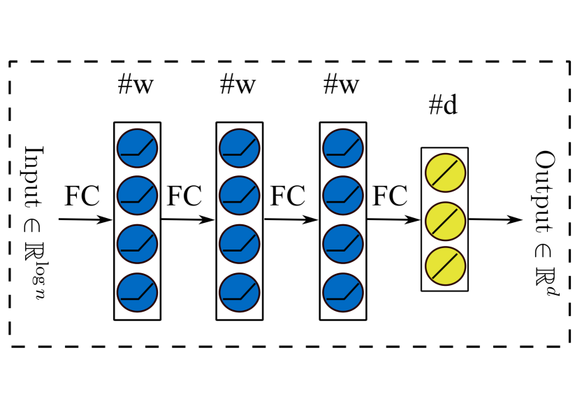
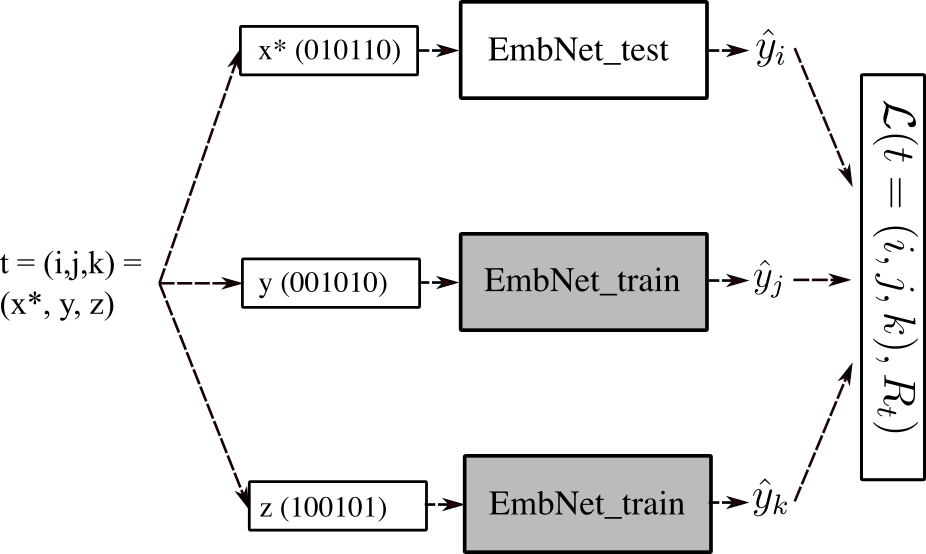
Our proposed architecture is inspired by the recent line of work on contrastive learning (Wang et al., 2014; Schroff et al., 2015; Cheng et al., 2016; Hoffer and Ailon, 2015). Figure 70(a) shows a sketch of our proposed network architecture. The central sub-module of our architecture is what we call the embedding network (EmbNet): one such network takes a certain encoding of a single data point as input (typically, an encoding of its index , see below) and outputs a -dimensional representation of data point . The EmbNet is replicated three times with shared parameters. The overall OENN network now takes the indices corresponding to a triplet as an input. It routes each of the indices to one of the copies of the EmbNet, which then return the -dimensional representations , respectively (cf. Figure 70(a)). The three sub-modules are trained jointly using the triplet hinge loss, as described by the following objective function:
| (9) |
Note that this optimization problem is not a relaxation to the OE problem. Rather, its an equivalent one Bower et al. (2018). Meaning that every global optima of this optimization problem is a feasible solution to the ordinal embedding problem and vice versa (up to a scale).
On the choice of input representation: Since we do not have access to any informative low-level input representations, the choice of input representations presents a challenge to this approach. However, we leverage the expressive power of neural networks (Leshno et al., 1993; Barron, 1993) and their ability to fit random labels to random inputs (Zhang et al., 2016) to motivate our choice of input encoding. Since our main goal is to find representations that minimize the training objective, we believe that completely arbitrary input representations are a viable choice.
One such input representation could be the one-hot encoding of the index (where point is encoded by a string of length such that if and otherwise). The advantage of choosing such a representation is that it is memory efficient in the sense that there is no need to additionally store the representations of the items. However, under this choice of representation the length of the input vectors grows linearly with the number of input items. As one of the central contributions of our work is to perform ordinal embedding in large scales, we consider a more efficient way: we represent each item by the binary code of its index, leading to a representation length of . Such a representation retains the memory efficiency of the one-hot encoding (in the sense as discussed above) but improves the length of the input representation from to . As we will see below, this representation works well in practice. However, note that there is nothing peculiar about this choice of binary code. Our simulations (see Subsection J.3) suggest that unique representations for items generated uniformly, randomly from a unit cube in can be used as the input encoding.
Structure of EmbNet: Figure 70(b) shows the schematic of the EmbNet. We propose a simple network with three fully-connected hidden layers and ReLu activation function. The final layer is a linear layer that takes the output of third hidden layer and produces the output embedding. The input size to the network is and each hidden layer contains nodes. The output layer has nodes to produce embeddings in . The input and output size, and , are pre-determined by the task. Thus the only independent parameter of the network is the width of hidden layers. Our experiments (see Subsection J.3) demonstrate that the hidden layer-width should grow logarithmically to the number of items to produce good embedding outputs.
Generalization to new data points: While the primary goal of embedding methods is to find a representation of the given training set, it is sometimes desirable to be able to extend the representation to new data points. A naive approach would be to re-train the OENN with the appropriate parameter settings (see Section J.3) with the combined set of training and test triplets. However, our approach features an elegant way to infer embeddings of a set of test items. Let denote a set of test items observed via a set of triplets of the form where at least one of the items in each triplet comes from and the rest could arise either from or . Such a triplet encodes the usual triplet relationship: is closer to than .
Our inference procedure (shown in Figure 70(c)) to obtain embeddings from is as follows. Recall that our architecture is composed of 3 identical EmbNet components with shared weights. Consider a OENN trained on and denote its (trained) EmbNet component as . We define to be an instance of with randomly re-initialized weights and to be an instance of with weights un-touched. The inference architecture, is then constructed dynamically for any triplet from in the following manner: items from in the triplet are provided as inputs to , while items from are provided as inputs to . We then proceed to train the network in the same fashion as before over except that we freeze the parameters of . Note that the training examples are unaffected in the inference procedure. The procedure produces embeddings of test items that satisfy the triplet constraints containing items both from and . Our experiments (Section J.4) indicate that the quality of embeddings provided by this procedure is quite satisfactory. We evaluate this using the triplet error.
Difference to previous contrastive learning approaches: As described earlier, our architecture is inspired by Wang et al. (2014); Hoffer and Ailon (2015). However, there are fundamental differences: 1) we have no access to representations for the input items and our network takes completely arbitrary representations for the input items. 2) In the previous work, triplets are always contrastive, which is of the form while simply gather triplets involving arbitrary sets of three points. Indeed, obtaining contrastive triplets requires additional information, either the class labels or more explicit similarity information between objects.
J.2 On the choice of the loss function
In our method, we use the hinge loss as the choice of our loss function. In what follows, we justify this choice by showing that the resulting optimization by using the hinge-loss does not constitute a relaxation to the ordinal embedding problem. Rather it’s an equivalent one.
The problem of ordinal embedding — finding an embedding that satisfies a set of given triplets, - can be phrased as a quadratic feasibility problem (Bower et al., 2018) as shown in Equation 10.
| (10) |
Each matrix corresponds to a triplet constraint that satisfies,
Every feasible solution to 10 is a valid solution to the problem of ordinal embedding.
An equivalent way to solve equation 10 (i.e., find a feasible solution of 10) is to find the global optima of the constrained optimization problem (Bower et al., 2018) given by equation 11:
| (11) |
This it true because every feasible solution to (10) can be scaled to attain global optima of (11) and every global optima of (11) is a feasible solution of (10) (Bower et al., 2018). Moreover, in optimization (1), any positive scaling of a feasible point is a solution to (1) as well, whereas in optimization (2) this effect is eliminated.
The hinge loss, therefore, satisfies the nice property that using the hinge loss to solve the ordinal embedding problem is not a relaxation but rather an equivalent problem.
J.3 Choice of parameters and hyper-parameters
Our network architecture depends on a few parameters: the number of layers , the width of the hidden layers , length of the input encoding and the dimension of the embedding space . To reduce the number of independent parameters of the network, we simply fix the number of layers to , where the number of units is the same in each of these layers. The embedding dimension is determined by the given task. Additionally, the training procedure requires the setting of a few hyper-parameters: choice of the optimizer, batch size, and learning rate. We use ADAM Kingma and Ba (2014) to train our network and use a batch size of and a learning rate of for all the experiments.
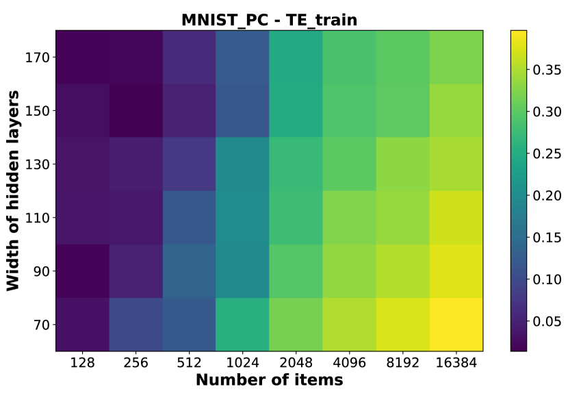
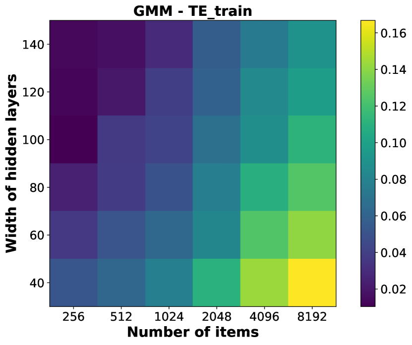
On the width of the hidden layers : The width of the hidden layers depends on the input dimension and the number of items . To investigate this dependence we use toy datasets where the dimension of the input space could be controlled. We ran simulations on 5 different datasets, specifically, we used the principal components of MNIST(Lecun and Cortes, 1998), USPS(Hull, 1994), CHAR(Dua and Graff, 2017), Mixture of Gaussian in and data sampled uniformly from a unit cube in .
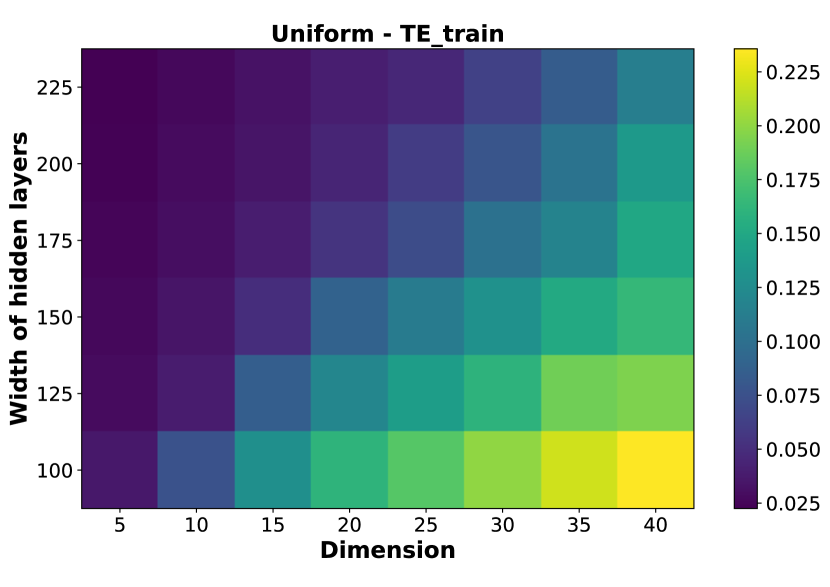
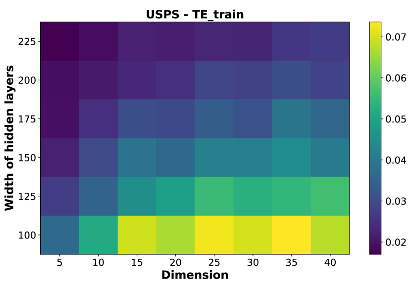
We perform two sets of experiments. First, we fix the number of points and generate datasets in an increasing number of dimensions, . We generate random triples from these datasets and use our model with increasing to embed them back into . Our simulations demonstrate that the width of the hidden layers needs to grow linearly with the embedding dimension. Similarly, fixing the input and the embedding dimension, our simulations demonstrate that needs to grow logarithmically with . Therefore, in all of our experiments, we set,
Dependence of the layer width on the number of items. Recall that in our setting, the neural network is used to solve a memorization task. The goal of the network is to fit completely arbitrary inputs — the index of the item — to outputs in . Therefore, it is reasonable to expect that with an increasing number of items, a larger network is required to address the complexity of the task. We can either increase the representational power of the network by adding more layers or by increasing the width of layers. We fix the number of layers to and investigate the dependence of layer width on .
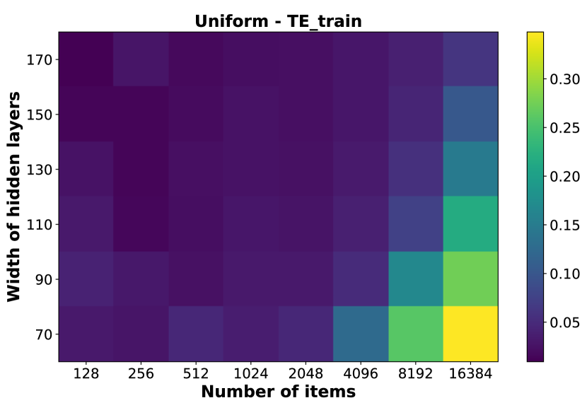
For each dataset, we choose an exponentially increasing number of items () in . Given a sample of points, we generate triplets (where is the embedding dimension). The embedding network (EmbNet) is constructed with 3 hidden layers, each having fully-connected neurons with ReLU activation functions. The width of the layers (= number of neurons in each layer) is increased linearly. For a fixed network and a fixed set of triplets, the experiment is executed 5 times in order to examine the average behavior of the model.
Figure 72 shows the training triplet error () of the ordinal embedding with varying number of items and width of the hidden layers for 3 different datasets. The error is reported by means of heat-maps, where warmer colors denote higher triplet error. Note that the axis increases exponentially and the axis increases linearly. The plots clearly establish logarithmic dependence of the hidden layer width on the number of items .
Dependence of the layer width on the embedding dimension
Besides the number of items, the embedding dimension is another factor that influences the complexity of ordinal embedding. We expect that the required layer width needs to grow with the embedding dimension. To investigate this dependence, as earlier, we sample items in from each dataset with varying input dimension . We generate triplets based on the Euclidean distances of items. To construct a network, the width of the layers is chosen from a linearly increasing set. For a fixed network and a fixed set of triplets, the experiment is executed 5 times in order to examine the average behavior of the model.
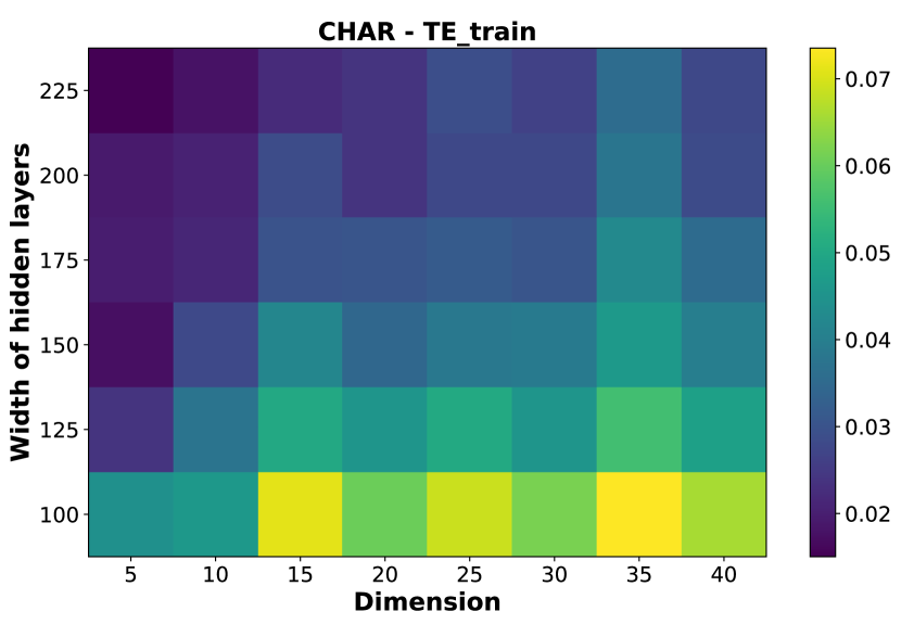
Figure 73 shows the training triplet error () of the ordinal embedding with varying dimensions and width of the hidden layers for 3 different datasets. There is again a clear line of transition between low and high error regions. In all of the datasets, it can be observed that the layer width has a linear dependence on the embedding dimension.
On the choice of the length of input encoding . The input to the OENN, as described earlier, can be chosen as a triplet of arbitrary encoding of the items. We ran simulations to establish the dependence of the length of such encoding with the number of items. These simulations show that the size of the input encoding needs to grow logarithmically with the number of items. In all the experiments, we set,
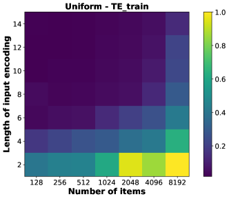
On the length of input encoding . Our algorithm takes random encoding of triplets of items as input and learns a transformation from the input encoding to vectors in Euclidean space of a dimension specified by the task. We run simulations with random input representations of a fixed length where we choose each component of the vector uniformly at random from the unit interval. Our simulations show that the size of the input encoding needs to grow logarithmically with an increasing number of items and using arbitrary representations of length suffices to achieve a small training triplet error (). To conduct the simulations, we sampled an exponentially increasing number of items uniformly from a unit square in . For a fixed set of items, we generate triplets (where is the dimension). To isolate the effect of the length of the input encoding, we construct our EmbNet by fixing the width of the hidden layer (). Figure 74 shows the training triplet error () of the ordinal embedding with varying number of items and the size of the input encoding. The result shows that logarithmic growth of the size of the input encoding with respect to suffices to obtain desirable performance.
J.4 Experiments on Generalization to new items
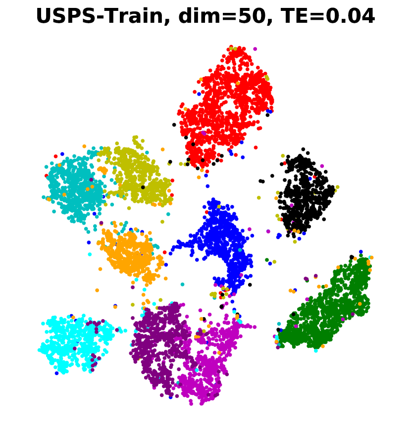
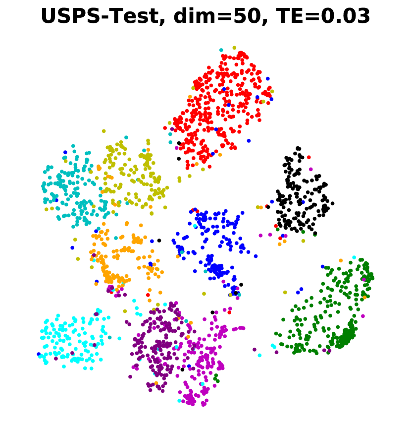
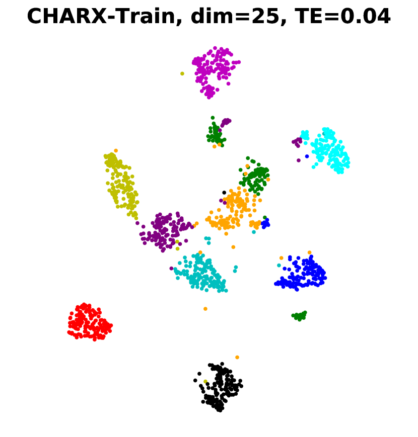
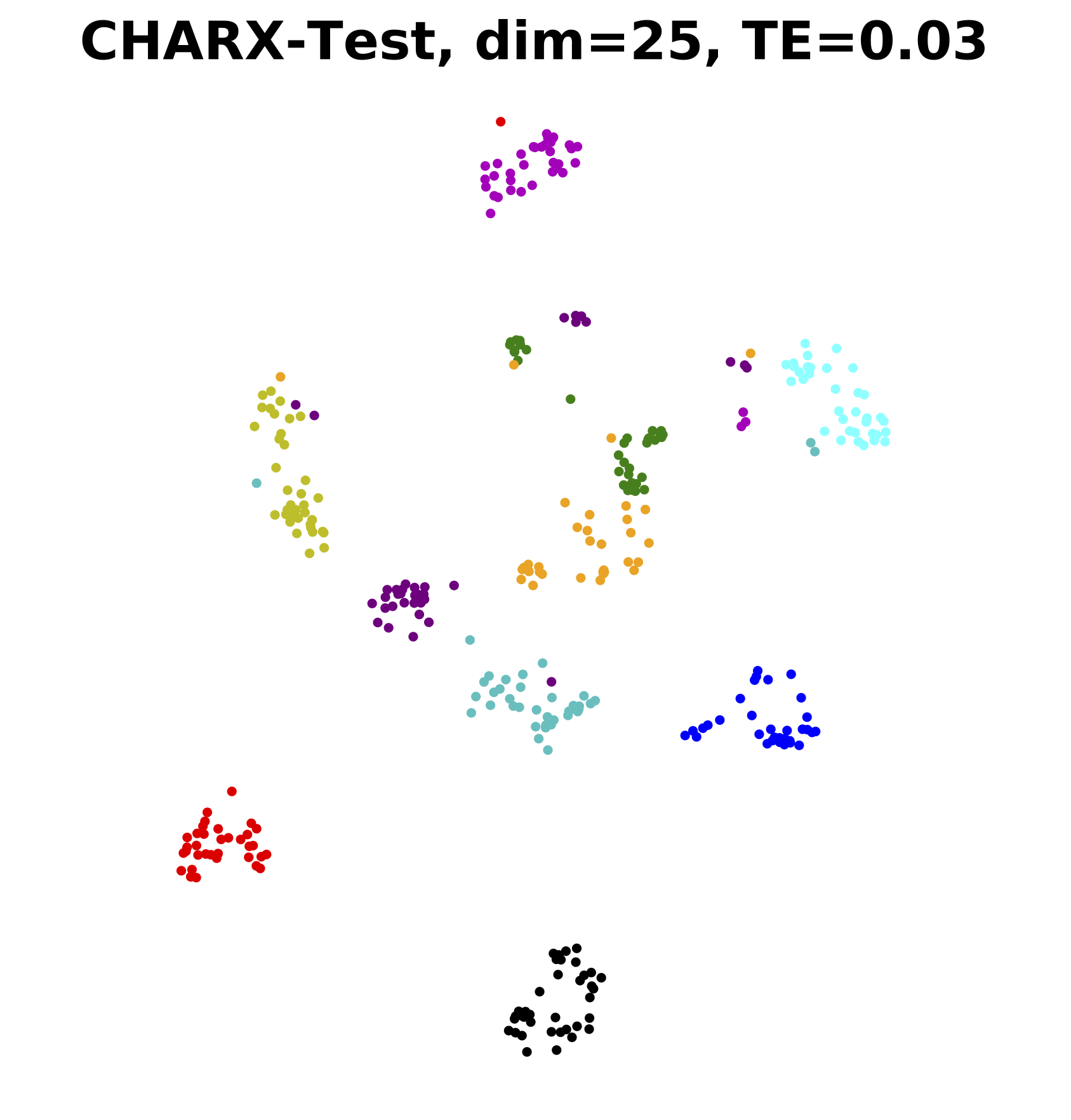
In this section, we present the performance of our method on out of sample extensions. To conduct this experiment, we choose the datasets USPS and CHAR. The USPS dataset has already a pre-defined training and test set. In the case of CHAR, we create the test set by randomly splitting the data into a train (80%) and a test set (20%). Subsequently, we generate triplets by drawing points uniformly at random from the train set of items. These triplets are then used to train the training network . Now we are going to study the out-of-sample extension. To this end, we randomly generate million triplets of items , where is always chosen from the test set and are drawn from the train set. The input representation of an item from the test set is chosen as the binary encoding of the index in length . The input representations for an item from the train set is chosen as the binary encoding of the index in length . Note that, the same indices are allowed to appear in the test set as well as the training set since different EmbNet components are used to generate the embeddings of items from the train set and the test set. Let denote the set of all triplets containing items from . The generalization network is then trained on (while keeping fixed as explained in the main paper). The results are demonstrated in Figure 71 by reporting both the fraction of triplets in that are not satisfied by and also by visualizing the output embeddings of both the training data and the test data in dimensions. The t-SNE algorithm is used to obtain the 2D visualization of the combined set of embeddings of both the train and the test items. The results clearly show that, in addition to satisfying all the triplets in , the quality of the obtained embeddings is high: the train and test embeddings look pretty much the same, and the triplet error is very low.
References
- Agarwal et al. (2007) S. Agarwal, J. Wills, L. Cayton, G. Lanckriet, D. Kriegman, and S. Belongie. Generalized non-metric multidimensional scaling. In AISTATS, 2007.
- Amid and Ukkonen (2015) E. Amid and A. Ukkonen. Multiview triplet embedding: Learning attributes in multiple maps. In ICML, 2015.
- Anderton and Aslam (2019) J. Anderton and J. Aslam. Scaling up ordinal embedding: A landmark approach. In ICML, 2019.
- Balcan et al. (2016) M. Balcan, E. Vitercik, and C. White. Learning combinatorial functions from pairwise comparisons. In COLT, 2016.
- Barron (1993) A. R. Barron. Universal approximation bounds for superpositions of a sigmoidal function. IEEE Transactions on Information Theory, 39(3):930–945, 1993.
- Bower et al. (2018) A. Bower, L. Jain, and L. Balzano. The landscape of non-convex quadratic feasibility. In ICASSP, 2018.
- Chang and Yeung (2008) H. Chang and D.Y. Yeung. Robust path-based spectral clustering. Pattern Recognition, 2008.
- Cheng et al. (2016) D. Cheng, Y. Gong, S. Zhou, J. Wang, and N. Zheng. Person re-identification by multi-channel parts-based cnn with improved triplet loss function. In CVPR, 2016.
- Choromanska et al. (2015) A. Choromanska, M. Henaff, M. Mathieu, G. B. Arous, and Y. LeCun. The loss surfaces of multilayer networks. In AISTATS, 2015.
- Clanuwat et al. (2018) T. Clanuwat, M. Bober-Irizar, A. Kitamoto, A. Lamb, K. Yamamoto, and D. Ha. Deep learning for classical japanese literature, 2018.
- De Silva and Tenenbaum (2004) V. De Silva and J. B. Tenenbaum. Sparse multidimensional scaling using landmark points. Technical report, Stanford University, 2004.
- Dua and Graff (2017) D. Dua and C. Graff. UCI machine learning repository, 2017. URL http://archive.ics.uci.edu/ml.
- Fränti and Sieranoja (2018) P. Fränti and S. Sieranoja. K-means properties on six clustering benchmark datasets, 2018. URL http://cs.uef.fi/sipu/datasets/.
- Ghosh et al. (2019) N. Ghosh, Y. Chen, and Y. Yue. Landmark ordinal embedding. In NeurIPS, 2019.
- Gionis et al. (2007) A. Gionis, H. Mannila, and P. Tsaparas. Clustering aggregation. ACM Transactions on Knowledge Discovery from Data (TKDD), 2007.
- Gower et al. (2004) J. C. Gower, G. B. Dijksterhuis, et al. Procrustes problems, volume 30. Oxford University Press on Demand, 2004.
- Haghiri et al. (2017) S. Haghiri, D. Ghoshdastidar, and U. von Luxburg. Comparison-based nearest neighbor search. In AISTATS, 2017.
- Haghiri et al. (2018) S. Haghiri, D. Garreau, and U. von Luxburg. Comparison-based random forests. In ICML, 2018.
- Heikinheimo and Ukkonen (2013) H. Heikinheimo and A. Ukkonen. The crowd-median algorithm. In HCOMP, 2013.
- Hoffer and Ailon (2015) E. Hoffer and N. Ailon. Deep metric learning using triplet network. In International Workshop on Similarity-Based Pattern Recognition, pages 84–92. Springer, 2015.
- Hull (1994) J. J. Hull. A database for handwritten text recognition research. IEEE Transactions on pattern analysis and machine intelligence, 1994.
- Jain et al. (2016) L. Jain, K. G Jamieson, and R. Nowak. Finite sample prediction and recovery bounds for ordinal embedding. In NeurIPS, 2016.
- Kawaguchi and Bengio (2019) K. Kawaguchi and Y. Bengio. Depth with nonlinearity creates no bad local minima in resnets. Neural Networks, 118:167–174, 2019.
- Kawaguchi et al. (2019) K. Kawaguchi, J. Huang, and L. Kaelbling. Effect of depth and width on local minima in deep learning. Neural Computation, 2019.
- Kingma and Ba (2014) D. Kingma and J. Ba. Adam: A method for stochastic optimization. arXiv preprint arXiv:1412.6980, 2014.
- Kleindessner and Luxburg (2015) M. Kleindessner and U. Luxburg. Dimensionality estimation without distances. In AISTATS, 2015.
- Kleindessner and von Luxburg (2014) M. Kleindessner and U. von Luxburg. Uniqueness of ordinal embedding. In COLT, 2014.
- Kleindessner and von Luxburg (2017) M. Kleindessner and U. von Luxburg. Kernel functions based on triplet comparisons. In NeurIPS, 2017.
- Kruskal (1964) Joseph B Kruskal. Multidimensional scaling by optimizing goodness of fit to a nonmetric hypothesis. Psychometrika, 29(1):1–27, 1964.
- Lecun and Cortes (1998) Y. Lecun and C. Cortes. The MNIST database of handwritten digits, 1998. URL http://yann.lecun.com/exdb/mnist/.
- Leshno et al. (1993) M. Leshno, V. Y. Lin, A. Pinkus, and S. Schocken. Multilayer feedforward networks with a nonpolynomial activation function can approximate any function. Neural networks, 6(6):861–867, 1993.
- Nguyen and Hein (2017) Q. Nguyen and M. Hein. The loss surface of deep and wide neural networks. In ICML, 2017.
- Paszke et al. (2019) A. Paszke, S. Gross, F. Massa, A. Lerer, J. Bradbury, G. Chanan, T. Killeen, Z. Lin, N. Gimelshein, L. Antiga, A. Desmaison, A. Kopf, E. Yang, Z. DeVito, M. Raison, A. Tejani, S. Chilamkurthy, B. Steiner, L. Fang, J.e Bai, and S. Chintala. Pytorch: An imperative style, high-performance deep learning library. In NeurIPS. 2019.
- Schroff et al. (2015) F. Schroff, D. Kalenichenko, and J. Philbin. Facenet: A unified embedding for face recognition and clustering. In CVPR, 2015.
- Shepard (1962) R. N. Shepard. The analysis of proximities: multidimensional scaling with an unknown distance function. i. Psychometrika, 27(2):125–140, 1962.
- Sieranoja and Fränti (2019) S. Sieranoja and P. Fränti. Fast and general density peaks clustering. Pattern Recognition Letters, 2019.
- Tamuz et al. (2011) O. Tamuz, C. Liu, S. Belongie, O. Shamir, and A. Kalai. Adaptively learning the crowd kernel. In ICML, 2011.
- Terada and von Luxburg (2014) Y. Terada and U. von Luxburg. Local ordinal embedding. In ICML, 2014.
- van der Maaten and Hinton (2008) L. van der Maaten and G. Hinton. Visualizing data using t-SNE. JMLR, 2008.
- van der Maaten and Weinberger (2012) L. van der Maaten and K. Weinberger. Stochastic triplet embedding. In Machine Learning for Signal Processing (MLSP), 2012.
- Wang et al. (2014) J. Wang, Y. Song, T. Leung, C. Rosenberg, J. Wang, J. Philbin, B. Chen, and Y. Wu. Learning fine-grained image similarity with deep ranking. In CVPR, 2014.
- Xiao et al. (2017) H. Xiao, K. Rasul, and R. Vollgraf. Fashion-mnist: a novel image dataset for benchmarking machine learning algorithms. arXiv preprint arXiv:1708.07747, 2017.
- Zahn (1971) C.T. Zahn. Graph-theoretical methods for detecting and describing gestalt clusters. IEEE Transactions on Computers, 1971.
- Zhang et al. (2016) C. Zhang, S. Bengio, M. Hardt, B. Recht, and O. Vinyals. Understanding deep learning requires rethinking generalization. ICLR, 2016.
- Zhang et al. (1997) T. Zhang, R. Ramakrishnan, and M. Livny. Birch: A new data clustering algorithm and its applications. Data Mining and Knowledge Discovery, 1997.