On particle-size distribution of convex similar bodies in
Abstract
We give an explicit form of particle-size distributions of convex similar bodies for random planes and random lines, which naturally generalize famous Wicksell’s corpuscle problem. The results are achieved by applying the Method of Model Solutions for solving well-known Santaló’s integral equations. We also give a partial result related to the question of existence and uniqueness of these solutions. We finally illustrate our approach on several examples.
keywords:
[class=MSC]keywords:
arXiv:0000.0000 \startlocaldefs \endlocaldefs
,
t1Supported by the Slovak Research and Development Agency under the contract No. APVV-16-0337.
1 Introduction
Stereology is originally concerned with the determination of three-dimensional structure from two-dimensional or one-dimensional observational data. It provides practical techniques for extracting quantitative information about this structure and is based on fundamental principles of geometry and statistics. It is a completely different approach from computed tomography, for which a complete set of all cross sections is needed. E.g. [1] sets out the principles of stereology from a statistical viewpoint, focusing on both basic theory and practical implications. It is an important and efficient tool in many applications of geology, metallurgy, petrology but also cell biology, petrography, materials science, histology or neuroanatomy.
In this article the general goal is the reconstruction of particles from cross sections in . We focus only on Santaló’s formulation, i.e. on the estimation problems concerned with ascertaining the size distribution of similarly shaped convex particles, capable of complete size specification by one size parameter and randomly distributed in a convex opaque field, see [10] or [4]. It also involves a famous original Wicksell’s corpuscle problem concerns the determination of the distribution of spherical particles from planar sections, see [12]. The solution was derived already in [12], but proven much later in [5]. This paper is organized as follows. We first present preliminaries in Section 2. In Section 3, we give an overview of the problem and introduce related integral equations that we want to solve. Sections 3.3 and 4 obtain most important result, an exact solutions for similar convex bodies for random planes and lines. The question of solvability is partially solved in Section 5. We illustrate our approach on several explicitly solved examples, see Sections 6 and 7. We put necessary technicalities in appendix.
2 Setup and preliminaries
Let be non-empty set. A complex random variable on the probability space is a map such that , where a are real random variables on (it can always be considered as pair of real random variables: its real and imaginary part). The -weighted space for measurable set is defined as
where , is a non-negative measurable function (weight) on and the set of all Lebesgue measurable functions. For simplicity, if , we do not write superscript or subscript. We also denote for fixed the space
where , whereas it it known that additionally an isometry holds. Similarly we set .
Now, recall that -th moment of real random variable is defined as
if the integral exists. Let us consider only random variables whose probability distributions are absolutely continuous, i.e. for distribution function we have for Here is a probability density function111Note that can be viewed as the probability that the random variable will fall within the infinitesimal interval , i.e. non-negative function from such that . It is good to realize that the Mellin transform defined by (B.1) in appendix B.1 of is -th moment of . In that case one has and necessarily . More generally for (Borel) measurable function it holds, that is a complex random variable and
with
(in the case of integrability). So for absolutely continuous complex random variable one has
We are dealing only with random variables with specific finite support, i.e.
where and , or for some . Obviously . We start with the following.
Lemma 2.1.
Let be a density of random variable . Then the moments does exist, are positive and
-
i)
for ;
-
ii)
for .
Moreover, for is moment a positive or . Also, and .
Proof.
Positiveness results from the fact that for (a.s.) one has Furthermore, for we obtain The estimate from below follows from Jensen’s inequality. Asymptotic property for follows from boundedness of the support and for from the fact that ∎
3 Particle-size distribution of a body based on its cut
Consider a convex body (compact convex set with non-empty interior) v containing a certain number of randomly placed, non-overlapping particles. Suppose that all of them are similar222By similarity on a metric space we assume a bijection such that for fixed . We call two sets similar if one is an image of the other according to similarity . to some convex body and their coefficient of similarity is . We denote a particle similar to as , so that . denotes its volume, surface area and the integral of the mean curvature333I.e. the average of the principal curvatures or equivalently defined using a divergence of the unit normal. of (its boundary). We omit the subscript when . Moreover, let be a number of particles per unit of volume in , whose coefficient of similarity is within the range
We intersect body with a random plane and a random line . Then the particles contained in , intersected by (), are the sections, convex domains in (intervals on ). Let and be the number of these sections of area and length in the range per unit area and per unit length, respectively. These values are random variables with densities and . However the area of and length of are also random variables with densities444 is the probability that the area of lies between and . is the probability that the length of lies between and . and . Set as a density of the area of and as a density of the length of , naturally . Moreover we have
| (3.1) |
| (3.2) |
see [10] or [4]. To find a is not in general a simple task. However, we assume that it is given and our problem is to find from and respectively. Notice that we have finite mean values of and respectively as they equal the following
3.1 Random plane intersection
For spherical case, see illustrative Figure 1. Denote as the maximal admissible value of , i.e. . We thus have that , and therefore
Example 3.1 (Spherical case).
In [10] is derived the integral relationship between and . We have for planes equation, which is of interest in this work:
| (RP) |
where is a constant (depending on e.g. ). Equation (RP) is a Volterra integral equation, where function depends on the shape of the body (and thus on the shape of all particles). Using the cross-sectional measurements of the body , it is possible to estimate the function , and then to derive from (RP). Notice if one finds then also has a distribution in given by .
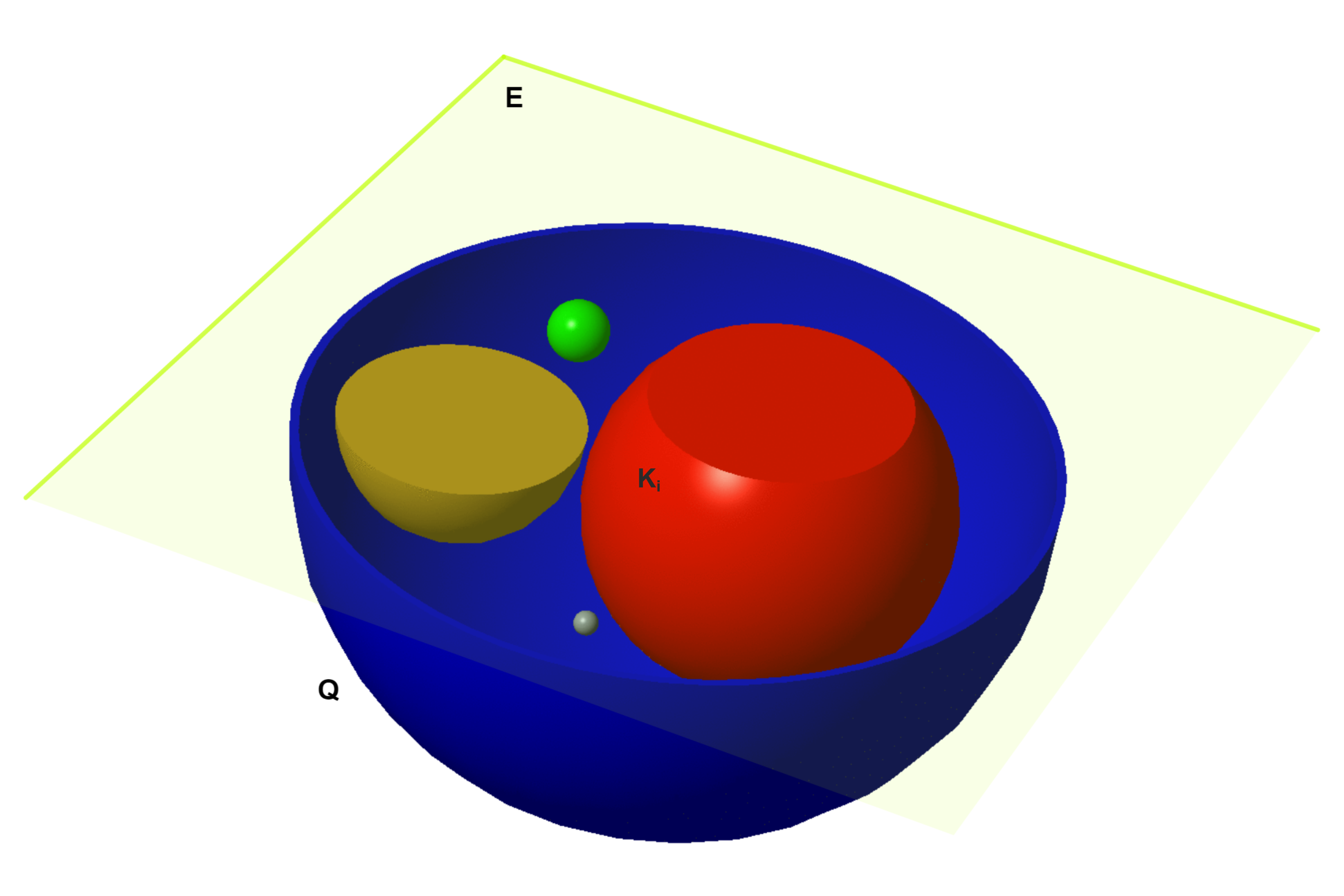
Example 3.2 (Continuation of the spherical case example 3.1).
Equation (RP) has the form
| (3.5) |
By using new variables , and we transform equation (3.5) to
| (3.6) |
which is known Abel integral equation555Its solution has the form (if it is well defined) (3.7) , whereas its integral corresponds to ”1/2 integration” but the unfolding problem is (moderately) ill posed. This yields the solution of original equation (3.5) in the form
| (3.8) |
Notice, that this form requires regularity of the input function .
Remark 3.1.
Consider now that the section diameter as random variable, whereas . Let be a density666 In the geometric meaning , it expresses the number of particles per unit area in , whose diameter in the cross-section is ., then
3.2 Correctness of a solution of (3.5), i.e. a spherical case
It can be verified that is a density if it is . However the non-negativity of does not guarantee the non-negativity of on the entire interval. The function must therefore satisfy the necessary condition that on the right neighborhood of zero. Notice that [8] they derive two conditions that must at least be met for the function to be a density. We introduce here in notation of transformed
| (3.12) |
whereas the first one is also necessary if and the second one if (it is even known that it is fulfilled if so for sufficiently fast).
3.3 Random line intersection
Here we continue analogously for random line case. See Figure 2, where spherical case is illustrated. Similarly we have and
Furthermore, the equation for random line intersection, see [10] or [4], is
| (RL) |
where . Again relation for distribution in variable is given by .
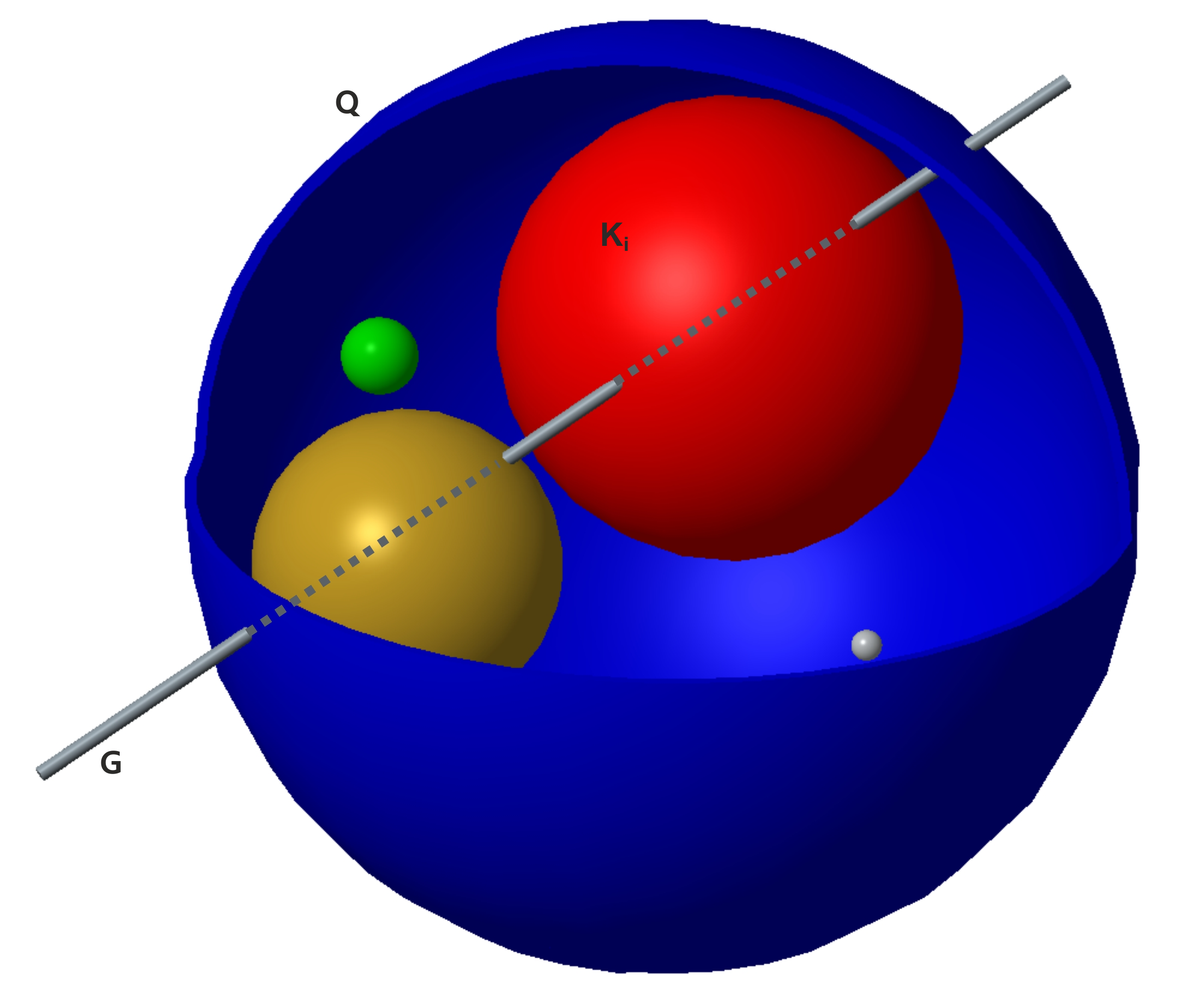
Example 3.3 (Spherical case).
We have () and , which yields that equation (RL) simplifies to
| (3.13) |
Equation (3.13) can be solved directly by differentiation with resulting form
| (3.14) |
In further we set the notation
| (3.15) |
Exact solutions for similar convex bodies for plane sections
In this section we find exact solution for random plane case. Consider here rewritten integral equation (RP)
where . We set in (RP) yielding an equation
| (3.16) |
We now seek a solution of equation (3.16) in the form . We have
| (3.17) |
This can be done by finding a relationship between and . Transformation convert equation (3.17) to
| (3.18) |
Considering the form of Mellin transform one has to have . We thus have or respectively. For simplicity we use the notation and similarly for function . Finally we have found :
| (3.19) |
Naturally (3.15) implies therefore and
| (3.20) |
solves equation (3.16), whereas
Now, we assume, which will be discussed later, that
Since solves equation (3.16) we simply obtain which gives
| (3.21) |
Linearity and interchanging of order of integration yield
| (3.22) |
We denote this solution as
| (3.23) |
4 Exact solutions for similar convex bodies for line sections
Now we focus on the random line case. Consider here rewritten integral equation (RL)
where . Again for in (RL) we have
| (4.1) |
with the assumption that its solution has the form . Similarly we obtain
| (4.2) |
and for
| (4.3) |
Once we set , we find
| (4.4) |
and the solution
| (4.5) |
of equation (4.1). Similarly as before is just
| (4.6) |
and
| (4.7) |
Finally
| (4.8) |
solves original equation (RL).
5 Existence of the solutions of equations (RP) and (RL)
Here we will consider the question of the existence of solutions of equations (RP) and (RL). In the context of integral equations, this is a difficult task, mainly because they are singular (albeit linear) equations. Notice that there is also statistical interpretation of their derived form. They have the form of inverse Mellin transformation of the ratio of moments and moments respectively, of random variables corresponding to the densities of and . Of course, the proportion of moments does not have to be a moment, so we cannot talk about a direct relationship to the new density. Indeed, for both equations, the non-negativity of the functions (inputs) and does not guarantee the non-negativity of the solution. Also, it can not be guaranteed that . Thus, none of the basic density properties need not be met even if the inputs are densities. For general inputs , determining the necessary or sufficient conditions is a very difficult problem (non-negativity, but also integrability property of the solution). Indeed, just look at the results for the spherical ones listed in 3.2. Nevertheless, we give here a partial answer. In further we denote as and
Proposition 5.1 (Random lines).
Proof.
Since , from Lemma 2.1 it follows that there exist and so, that . Thus from Theorem B.2 we have and . This means, that for which is less than 1 therefore . Again from Lemma 2.1 we have that, is nonzero and thus the quotient which means that the necessary condition for this function to be Mellin’s image is fulfilled. Since , from Theorem B.4 it follows that is well defined. Furthermore, it follows from Fubini’s theorem and transformation theorem that
Since , from the inverse theorem B.7 we get that a.e. This guarantees the existence since a.e. equal functions have the same Mellin’s image. Now, if and solves given equation, then equality implies uniqueness, since a.e. The second part of the proposition follows from Theorems B.5 and B.6. ∎
The proof of the following proposition is identical to the previous one.
Proposition 5.2 (Random planes).
Notice that for we have sufficient conditions for the solutions and to be in . It is good to realize that we can say more. Indeed, independence of Mellin’s inversion on (for which can be integrated) must necessarily follow from the uniqueness of Mellin transform. Thus, if it fulfills the condition of uniform convergence (B.2), then and are in for some interval
6 Random plane examples
Recall that we have two formulas, that give us solution of the integral equation (RP), in spherical case, the classical one (3.8) and our formula (3.23). In this section we show that the former one can not be used when violating regularity of the right hand site.
Example 6.1 (Nearly spherical case).
It is a natural generalization of spherical case (i.e. when ) with the density kernel
| (6.1) |
where and . This leads to generalized Abel integral equation and similar type of solution of the form
| (6.2) |
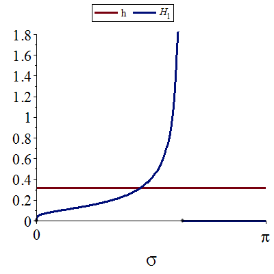
see e.g. [10]. Again regularity condition on is needed. See Figure 3 for case of .
The following example shows that the original formula derived formally (Abel integral equation) is not always applicable. Recall that Beta function is defined as and .
Example 6.2 (Spherical case, uniform distribution).
Consider the equation (RP) and uniform density in the form
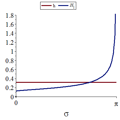
First we find and :
Example 6.3 (Nearly spherical case, uniform distribution).
For uniform density
and density given by (6.1) one can show that the solution has normalized form (i.e. it is a density)
7 Random line examples
In this section we give several examples of solutions of the integral equation (RL). Recall that we have two formulas in spherical case, i.e. classical (3.14) and our formula (4.8). In this case they coincide.
Example 7.1 (Spherical case, triangle distribution).
This example shows that the support of resulting density need not be full original set. Consider equation (RL) the density in the form
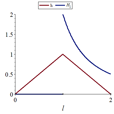
Example 7.2 (Spherical case, quadratic distribution).
Again consider equation (RL) and right hand site in the form
Again a.e. but notice that this solution is not integrable (thus it can not be normalized in standard sense).
Acknowledgements
This work was supported by the Slovak Research and Development Agency under the contracts No. APVV-16-0337 and APVV-17-0568.
References
- Baddeley and Jensen [2004] {bbook}[author] \bauthor\bsnmBaddeley, \bfnmA.\binitsA. and \bauthor\bsnmJensen, \bfnmE. B. V.\binitsE. B. V. (\byear2004). \btitleStereology for Statisticians. \bseriesChapman & Hall/CRC Monographs on Statistics & Applied Probability. \bpublisherTaylor & Francis. \endbibitem
- Bertrand and Ovarlez [2018] {binbook}[author] \bauthor\bsnmBertrand, \bfnmJ. Bertrand P.\binitsJ. B. P. and \bauthor\bsnmOvarlez, \bfnmJ. P.\binitsJ. P. (\byear2018). \btitleThe Mellin Transform. In \bbooktitleTransforms and Applications Handbook. \bseriesElectrical Engineering Handbook \bchapter12. \bpublisherCRC Press. \endbibitem
- Butzer and Jansche [1997] {barticle}[author] \bauthor\bsnmButzer, \bfnmPaul L.\binitsP. L. and \bauthor\bsnmJansche, \bfnmStefan\binitsS. (\byear1997). \btitleA direct approach to the mellin transform. \bjournalJournal of Fourier Analysis and Applications \bvolume3 \bpages325–376. \bdoi10.1007/BF02649101 \endbibitem
- De-Lin [1994] {bbook}[author] \bauthor\bsnmDe-Lin, \bfnmRen\binitsR. (\byear1994). \btitleTopics in integral geometry \bvolume19. \bpublisherWorld Scientific Publishing Company. \endbibitem
- Enderlein [1965] {barticle}[author] \bauthor\bsnmEnderlein, \bfnmG.\binitsG. (\byear1965). \btitleKendall, M. G., and P. A. P. Moran: Geometrical Probability. Griffin, London 1963; 125 S., Preis 28 s. \bjournalBiometrische Zeitschrift \bvolume7 \bpages208-208. \bdoi10.1002/bimj.19650070322 \endbibitem
- Flajolet, Gourdon and Dumas [1995] {barticle}[author] \bauthor\bsnmFlajolet, \bfnmPhilippe\binitsP., \bauthor\bsnmGourdon, \bfnmXavier\binitsX. and \bauthor\bsnmDumas, \bfnmPhilippe\binitsP. (\byear1995). \btitleMellin transforms and asymptotics: Harmonic sums. \bjournalTheoretical computer science \bvolume144 \bpages3–58. \endbibitem
- Gabutti and Sacripante [1991] {barticle}[author] \bauthor\bsnmGabutti, \bfnmB.\binitsB. and \bauthor\bsnmSacripante, \bfnmL.\binitsL. (\byear1991). \btitleNumerical inversion of the Mellin transform by accelerated series of Laguerre polynomials. \bjournalJournal of Computational and Applied Mathematics \bvolume34 \bpages191 - 200. \bdoihttps://doi.org/10.1016/0377-0427(91)90041-H \endbibitem
- Gorenflo and Vessella [1980] {barticle}[author] \bauthor\bsnmGorenflo, \bfnmRudolf\binitsR. and \bauthor\bsnmVessella, \bfnmSergio\binitsS. (\byear1980). \btitleAbel integral equations(analysis and applications). \bjournalLecture Notes in Mathematics. \endbibitem
- Oberhettinger [2012] {bbook}[author] \bauthor\bsnmOberhettinger, \bfnmF.\binitsF. (\byear2012). \btitleTables of Mellin Transforms. \bpublisherSpringer Berlin Heidelberg. \endbibitem
- Santaló [1976] {bbook}[author] \bauthor\bsnmSantaló, \bfnmLuis\binitsL. (\byear1976). \btitleIntegral geometry and geometric probability. With a foreword by Mark Kac., \bedition1. ed. \bpublisherAddison‐Wesley Publishing Company. \endbibitem
- Tsamasphyros and Theocaris [1976] {barticle}[author] \bauthor\bsnmTsamasphyros, \bfnmG.\binitsG. and \bauthor\bsnmTheocaris, \bfnmP. S.\binitsP. S. (\byear1976). \btitleNumerical inversion of Mellin transforms. \bjournalBIT Numerical Mathematics \bvolume16 \bpages313–321. \bdoi10.1007/BF01932274 \endbibitem
- Wicksell [1925] {barticle}[author] \bauthor\bsnmWicksell, \bfnmS. D.\binitsS. D. (\byear1925). \btitleThe corpuscle problem. A mathematical study of a biometric problem. \bjournalBiometrika \bvolume17 \bpages84-99. \bdoi10.1093/biomet/17.1-2.84 \endbibitem
- Yakubovich [1996] {bbook}[author] \bauthor\bsnmYakubovich, \bfnmS. B.\binitsS. B. (\byear1996). \btitleIndex Transforms. \bpublisherWorld Scientific. \endbibitem
Appendix A The Method of Model Solutions
Consider a linear equation in the operator form
| (A.1) |
where linear (integral) operator777 has to be independent of , is an unknown function, and is a known function. Let us have a (non constant) test solution
| (A.2) |
depending on an auxiliary parameter . The right-hand side that corresponds to the test solution (A.2) is
| (A.3) |
Let us multiply equation (A.3) by some function and integrate it with respect to over an suitable interval . Assumption of the interchange of the order of integration yields
| (A.4) |
with
| (A.5) |
Then from and follows, for the right-hand side , that the function is a solution of the original equation . Here the main problem is how to choose a function to obtain a given function . This can be overcome by finding a test solution (called a model solution) such that the right-hand side of is the kernel of a known inverse integral transform.
Appendix B Mellin transform
The following section discusses Mellin integral transform and its properties. In the text we rely mainly on works [3] and [6]. In our problem of solving (RP) and (RL), using Mellin transform seems paradoxically easier that using Laplace or Fourier.
Denote as an open strip of complex number such, that (to be more precise , thus a vertical strip parallel with the imaginary axis intersecting the real axis in a ). For the Mellin transform is defined as
| (B.1) |
Largest open strip of its convergence is called fundamental strip. Since , we have . To emphasize for fixed notation of transform (B.1) is used. It is well known that (absolute) convergence on is determined by asymptotical behaviour near 0 and :
A lot of examples can be found in monograph [9] consisting of, a.o., the Mellin and inverse Mellin transformation tables. We will now present basic properties we need. The set of holomorphic functions on open is denoted as
Theorem B.1 ([3], Pr. 1).
-
a)
Mellin transform is bounded linear operator on , so that .
-
b)
If and , then a , whereas
Theorem B.2 ([3], Th. 1.).
If then .
Theorem B.3 ([13], Th. 1.15.).
If for some , then exists and belongs into .
E.g. yields . On the other hand, when we talk about transformation, we also need to talk about its inversion and we naturally ask if ? Here we have to emphasize that the Mellin transform does not map functions from into surjectively. Indeed, there is no image, for example, for a holomorphic function . Necessary condition for to be the Mellin transform of a function from , is
| (B.2) |
uniformly with respect to . From the further it follows that the condition (B.2) it is also sufficient if . For is the inverse Mellin transform defined as
| (B.3) |
It is well defined as the next theorem says.
Theorem B.4 ([3], Pr. 5., Lm. 4.).
Is is also fact, that if the function is holomorphic and vanishes sufficiently fast for , then the Cauchy integral theorem yields that the inverse888It is good to realize that from a practical point of view the inverse Mellin transformation formula (B.4) is not easy to use and usually leads to relatively complicated calculations (using, for example, the theory of complex analysis). (B.3) is in fact a (complex) path integral (along a line parallel to the -axis) given by
| (B.4) |
If we add boundedness to holomorphy property, we can say something about the continuity of images of the transform.
Theorem B.5 ([2], Th. 12.1.).
If and if does exist such that , then
We may also be interested when the image of the transform will be in some of the spaces .
Theorem B.6 ([13], Th. 1.16.).
If for some , then exists and belongs into .
Here is an important inversion theorem.
Theorem B.7 ([3], Th. 7., 8.).
-
a)
If and for some , then a.e. on (if moreover , then it holds ).
-
b)
If and for every , then
-
c)
If for some such that , then a.e. on .