IFUP-TH-2019
Deuteron electric dipole moment from holographic QCD

Abstract

We compute the electric dipole moment (EDM) of the deuteron in the holographic QCD model of Witten-Sakai-Sugimoto. Previously, the leading contribution to the EDM of nucleons was computed, finding opposite values for the proton and the neutron which then cancel each other in the deuteron state. Here we compute the next-to-leading order contribution which provides a splitting between their absolute value. At large ${N_{\rm c}}$ and large ’t Hooft coupling $\lambda$, nuclei are bound states of almost isolated nucleons. In particular, we find that in this limit the deuteron EDM is given by the splitting between proton and neutron EDMs. Our estimate for the deuteron EDM extrapolated to the physical values of ${N_{\rm c}}$, $\lambda$, $M_{\mathop{KK}\nolimits}$ and $m_{q}$ is $d_{d}=-0.92\times 10^{-16}\theta\ e\cdot{cm}$. This is consistent, in sign and magnitude, with results found previously in the literature and obtained using completely different methods.

1 Introduction

The action of QCD can be supplemented with a topological $\theta$-term without spoiling its gauge and Lorentz invariance: this term however introduces CP-violation in the theory, as it can be regarded as an analog of the $\vec{B}\cdot\vec{E}$ term in electromagnetism.

The most studied CP-violating observables arising from this term are electric dipole moments of baryons, $\mathcal{D}_{B}$, that are linear in the $\theta$-parameter. Until recent years, following the pioneering work of Ramsey and Purcell in 1950 [1], most efforts were directed at predicting the electric dipole moment of the neutron $\mathcal{D}_{\rm n}$, which was the most accessible one using direct measures: Experimentally an upper bound amounting to $|\mathcal{D}_{\rm n}|<3.0\times 10^{-26}e\cdot cm$ has been established for this observable [2], while most estimates set the value of the $\theta$-induced contribution to the dipole moment to about $10^{-16}\theta e\cdot cm$. This implies a somewhat unnatural smallness for the $\theta$ parameter, which is then set to less than about $\theta\lesssim 10^{-10}$. This unnaturally small, but eventually nonvanishing amount of CP-violation goes under the name of the “strong CP-problem”.

For the deuteron, the state-of-the-art of the electric dipole moment $\mathcal{D}_{\rm D}$ is less rich at the moment. On the experimental side especially there are no direct measures due to the fact that it is electrically charged, making it unfit for measurements which involve placing it in electric fields. Theoretical estimates are essentially obtained through QCD sum rules [3, 4] and via models of nuclear potential [5] : the tool that provided most estimates for $\mathcal{D}_{\rm n}$, the chiral Lagrangian, tends to produce electric dipole moments that are equal in magnitude and opposite in sign for the neutron and the proton, so that the single nucleon contributions, which are expected to be important, tend to cancel each other inside the deuteron: nevertheless some results in this context are available for the $\theta$ induced EDM as lower bounds [7, 8], while two-nucleon terms can also be computed [9, 10].

In recent years both the experimental and theoretical fields have acquired new tools to tackle the problem of the determination of $\mathcal{D}_{\rm D}$. On the experimental side, the development of storage-ring technology allows to measure the electric dipole moment of charged particles with relevant precision: The JEDI collaboration in Jülich has a goal of reaching a potential sensitivity of $10^{-29}\text{e}\cdot\text{cm}$ [11], so that there is the possibility, if good theoretical predictions are available, that the strong CP-problem can be pushed to even more restrictive regimes, lowering the upper bound on $\theta$. The other possibility is that instead the experiments find a finite value for $\mathcal{D}_{\rm D}$, in which case it would be of paramount importance to have a quantitatively meaningful theoretical estimate, to infer the value of $\theta$.

On the theory side instead, the holographic model of Witten-Sakai-Sugimoto (WSS) [12, 13, 14] has been used to successfully compute the electric dipole moments of the neutron and the proton [15, 16]: Despite the computation leading to the old chiral Lagrangian cancellation issue ($\mathcal{D}_{\rm n}=-\mathcal{D}_{\rm p}$), the result was obtained at leading order in few parameters of the theory, in particular neglecting time derivatives, leaving open the possibility of the appearance of a splitting in the magnitudes of the electric dipole moments of the nucleons at the next-to-leading order or beyond.

It is not a simple task to make an estimate of $\mathcal{D}_{B}$ since it lies beyond the possibilities of the usual perturbative approach to QCD, and even the lattice approach is tricky due to the presence of the sign problem (as examples of a lattice estimate, see Refs. [17, 18, 19, 20]): throughout the years, many attempts with effective theories, such as the chiral Lagrangian [21] and the Skyrme model [22, 23] have achieved some good estimates for the neutron. Since the introduction of the $AdS/CFT$ duality by Maldacena in 1997 [24], it has been a major goal for theoretical physicists to develop a holographic theory of QCD which could then be used to explore its rich non-perturbative sector: the model which has achieved the best degree of success so far is that of Witten-Sakai-Sugimoto.

The WSS model is based on a $D4$–$D8$ brane setup in type IIA string theory. In the limit where a simple holographic dual description is given, the model reduces to a $3+1$ dimensional large-${N_{\rm c}}$ $SU({N_{\rm c}})$ gauge theory with ${N_{\rm f}}$ massless quarks. Additionally, it also contains a tower of massive adjoint matter fields whose mass scale is set by a dimensionful parameter denoted as $M_{\mathop{KK}\nolimits}$ (which gives the scale of the glueballs as well). Despite this feature, at low energies, the model shares all the expected features with QCD, like confinement, chiral symmetry breaking and so on. The WSS is the top-down holographic theory closest to QCD. It incorporates automatically the whole tower of vector mesons and exhibits complete vector dominance in the hadron electromagnetic form factors. It has very few parameters to fit. Flavor dynamics is encoded in the low-energy action for the gauge field on the flavor branes, and the baryons of QCD are instantonic configurations of that gauge theory [25, 26, 27, 28]. Quantization of the degrees of freedom for an instantonic field of charge one creates a quantum system of states, whose transformation properties and quantum numbers are just right to interpret them as nucleons. Nuclear physics at low energy is thus turned into a multi-instanton problem in a curved five-dimensional background.

Just like baryons in the large-${N_{\rm c}}$ limit can be seen as solitons of the chiral Lagrangian, in the WSS model they are identified with instantons of the holographic Lagrangian describing the mesonic sector [26, 25].

If quarks are massless, any $\theta$-dependence is washed out by a chiral rotation of the quarks. A (small) mass term for the quarks can be introduced using a prescription suggested in Refs. [29, 30].

In this work we use the WSS model, supplemented with a finite quark mass, to carry out a novel independent computation of $\mathcal{D}_{\rm D}$ from first principles: i.e. the model of Witten-Sakai-Sugimoto adopts a top-down approach, which provides us with valuable physical insights through the calculations performed. It is, to our knowledge, the first holographic attempt at performing this task.

The paper is organized as follows. In Section 2 we will review the main features of the nucleons in the WSS model, the inclusion of the $\theta$ term and the electric dipole moment. In Section 3 we perform the next-to-leading order analysis. In Section 4 we use the newly found perturbations to compute their contributions to the nucleon EDM showing that it is of isoscalar nature. In Section 5 we relate the EDMs of the nucleons to that of the deuteron. We conclude in Section 6. In Appendix A we provide the explicit form of all the equations. In Appendix B we describe the numerical solution.

2 Holographic QCD, nucleons and EDM

2.1 Background and effective action

The starting point in the construction of the model is Witten’s confining background in type IIA supergravity: it is generated by a stack of ${N_{\rm c}}$ coincident $D4$-branes, which encode color degrees of freedom, making the theory holographically dual to $SU({N_{\rm c}})$ Yang-Mills. The field content of the background includes the metric, the dilaton and the Ramond-Ramond three-form $C_{3}$:

$$\begin{split}ds^{2}&=\left(\frac{u}{R}\right)^{3/2}\left(\eta_{\mu\nu}dx^{\mu}dx^{\nu}+f(u)dx_{4}^{2}\right)+\left(\frac{R}{u}\right)^{3/2}\left(\frac{du^{2}}{f(u)}+u^{2}d\Omega_{4}^{2}\right),\\ e^{\phi}&=g_{\rm s}\left(\frac{u}{R}\right)^{3/4},\quad\quad F_{4}=dC_{3}=\frac{2\pi{N_{\rm c}}}{\mathop{Vol}\nolimits_{4}}\epsilon_{4},\quad\quad f(u)=1-\frac{u_{\mathop{KK}\nolimits}^{3}}{u^{3}}.\end{split}$$ (2.1)

The $x_{4}$ and $u$ directions form a subspace with the shape of a “cigar”, as can be seen from the fact that the geometry ends smoothly at a finite value of the $u$ coordinate, viz. $u=u_{\mathop{KK}\nolimits}$. The $x_{4}$ direction is compactified on an $S^{1}$ whose radius shrinks to zero at $u=u_{\mathop{KK}\nolimits}$: absence of conical singularities fixes the periodicity of the $x_{4}$ coordinate in terms of the radius of the background $S^{4}$ (given by $R$ and fixed by the flux of $F_{4}$) and the value of $u_{\mathop{KK}\nolimits}$ which is a free parameter. The relation is given by

$$\delta x_{4}=\frac{4\pi}{3}\frac{R^{3/2}}{u_{\mathop{KK}\nolimits}^{1/2}}\equiv\frac{2\pi}{M_{\mathop{KK}\nolimits}},$$ (2.2)

where we have traded the free parameter $u_{\mathop{KK}\nolimits}$ for another one, i.e. the energy scale $M_{\mathop{KK}\nolimits}$ that defines the radius of $x_{4}$. It is useful to work in units such that

$$M_{\mathop{KK}\nolimits}=u_{\mathop{KK}\nolimits}=1,$$ (2.3)

that is to say that we measure distances and energies in units of $M_{\mathop{KK}\nolimits}^{-1}$ and $M_{\mathop{KK}\nolimits}$. Restoring the factors of $M_{\mathop{KK}\nolimits}$ at the end of the computations will be easy using simple dimensional analysis.

The inclusion of flavor degrees of freedom is performed via the addition of two stacks of ${N_{\rm f}}$ $D8/\overline{D8}$-branes in the probe regime: we engineer them to be localized in the $x_{4}$ direction and antipodal on the $S^{1}$. This way the branes are found to merge into a single stack at the cigar tip, realizing a holographic version of chiral symmetry breaking. It is then useful to trade the bulk coordinate $u$ with one that runs on the $D8$ world volume, call it $z$, related by (in the antipodal setup)

$$\left\{\begin{aligned} \quad&u^{3}=u_{\mathop{KK}\nolimits}^{3}+u_{\mathop{KK}\nolimits}r^{2}\\ \quad&x_{4}=\frac{2R^{3/2}}{3u_{\mathop{KK}\nolimits}^{1/2}}\theta\end{aligned}\right.\quad\Rightarrow\quad\left\{\begin{aligned} \quad&y=r\cos\theta\\ \quad&z=r\sin\theta\end{aligned}\right.$$ (2.4)

The effective action at low energies is then given by the $D8$-branes world-volume action in the curved background generated by the $D4$-branes: after a trivial dimensional reduction on $S^{4}$, it amounts to a Yang-Mills and Chern-Simons theory on a five-dimensional curved space

$$S = S_{\mathop{YM}\nolimits}+S_{\mathop{CS}\nolimits},$$

$$S_{\mathop{YM}\nolimits} = -\kappa\mathop{Tr}\nolimits\int d^{4}xdz\left[\frac{1}{2}h(z)\mathcal{F}_{\mu\nu}^{2}+k(z)\mathcal{F}_{\mu z}^{2}\right],$$ (2.5)

$$S_{\mathop{CS}\nolimits} = \frac{{N_{\rm c}}}{384\pi^{2}}\epsilon_{\alpha_{1}\alpha_{2}\alpha_{3}\alpha_{4}\alpha_{5}}\int d^{4}xdz\widehat{A}_{\alpha_{1}}\left[6\mathop{tr}\nolimits\left(F_{\alpha_{2}\alpha_{3}}^{a}F_{\alpha_{4}\alpha_{5}}^{a}\right)+2\mathop{tr}\nolimits\left(\widehat{F}_{\alpha_{2}\alpha_{3}}\widehat{F}_{\alpha_{4}\alpha_{5}}\right)\right],$$

where $\kappa\equiv a{N_{\rm c}}\lambda$ with $a\equiv(216\pi^{3})^{-1}$, and $k(z)=(1+z^{2})$, $h(z)=k(z)^{-1/3}$. In Eq. (2.1) we introduced the $D8$ gauge field $\mathcal{A}$, a $U({N_{\rm f}})$ connection which we expand as

$$\mathcal{A}=\widehat{A}\frac{\mathds{1}}{\sqrt{2{N_{\rm f}}}}+A^{a}T^{a},$$ (2.6)

where $T^{a}$ are the generators of $SU({N_{\rm f}})$ normalized as $\mathop{tr}\nolimits(T^{a}T^{b})=\frac{1}{2}\delta^{ab}$ (i.e. $T^{a}=\frac{\tau^{a}}{2}$ in the ${N_{\rm f}}=2$ case). We adopt the following notation for space and time indices: $\alpha$ labels all of the five directions of the effective spacetime ($\alpha=0,\ldots,3,z$), Greek letters $\mu,\nu$ label the four-dimensional spacetime but not the bulk coordinate ($\mu,\nu=0,\ldots,3$), capital Latin letters label all spatial directions ($M,N,\ldots=1,2,3,z$), while small Latin letters are reserved for the three spatial directions that do not extend into the bulk ($i,j,\ldots=1,2,3$).

2.2 Baryons as holographic solitons

Despite the model having mesons as fundamental degrees of freedom, it can successfully describe baryons as a solitonic configuration with a nontrivial instanton number. From a string theory point of view, this would correspond to a $D4$-brane wrapped on $S^{4}$, with ${N_{\rm c}}$ fundamental strings connecting it to the color branes.

An approximate solution [26] is found by restricting the analysis to a region near the cigar tip, where the warp factors $h(z)$ and $k(z)$ can be approximated by unity. This is a good approximation in the large $\lambda$ limit since the baryon size is found to be of order $\lambda^{-1/2}$. The static configuration is given by the $SU(2)$ BPST instanton in flat space, with the addition of an electromagnetic potential in the Abelian sector:

$$A_{M}^{\rm cl}=-if(\xi)g\partial_{M}g^{-1},\quad\quad\widehat{A}_{0}=\frac{{N_{\rm c}}}{8\pi^{2}\kappa}\frac{1}{\xi^{2}}\left[1-\frac{\rho^{4}}{(\xi^{2}+\rho^{2})^{2}}\right],\quad\quad A_{0}=\widehat{A}_{M}=0,$$ (2.7)

with

$$f(\xi)=\frac{\xi^{2}}{\xi^{2}+\rho^{2}},\quad\quad g=\frac{\left(z-Z\right)-i\left(\vec{x}-\vec{X}\right)\cdot\vec{\tau}}{\xi},\quad\quad\xi^{2}=\left(z-Z\right)^{2}+|\vec{x}-\vec{X}|^{2}.$$ (2.8)

Note that $\rho$ and $Z$ are not real moduli of the soliton since they have a potential

$$U(\rho,Z)=8\pi^{2}\kappa\left(1+\frac{\rho^{2}}{6}+\frac{{N_{\rm c}}^{2}}{5(8\pi^{2}\kappa)^{2}\rho^{2}}+\frac{Z^{2}}{3}\right),$$ (2.9)

which is minimized by the classical values

$$\rho^{2}_{\rm cl}=\frac{{N_{\rm c}}}{8\pi^{2}\kappa}\sqrt{\frac{6}{5}},\quad\quad Z_{\rm cl}=0.$$ (2.10)

Time dependence can be implemented in the moduli of the soliton: $X^{M}(t)$ describes the position of the center of mass in four-dimensional space, $\rho(t)$ is the instanton size, $y_{I}(t)$ describe the $SU(2)$ orientation: $y_{I}$ and $\rho$ are not independent, they are actually related by $\sum y_{I}^{2}=\rho^{2}$, so it is useful to introduce $a_{I}\equiv y_{I}/\rho$. Other than promoting the moduli to be time-dependent quantities, a transformation on the static gauge fields is also implemented: it looks like a gauge transformation, but it is not since it does not act on the $A_{0}$ field:

$$A_{M}=VA_{M}^{\rm cl}V^{-1}-iV\partial_{M}V^{-1}.$$ (2.11)

This way the field strength transforms as:

$$F_{MN} = VF_{MN}^{\rm cl}V^{-1},$$

$$F_{0M} = V\left(\dot{X}^{\alpha}\partial_{\alpha}A_{M}^{\rm cl}-D_{M}^{\rm cl}\Phi\right)V^{-1},$$ (2.12)

with $\Phi$ given by

$$\Phi\equiv-iV^{-1}\dot{V}.$$ (2.13)

To find a solution for $V(x,t)$ requires to find the function $\Phi(x,t)$ and perform a path-ordered integration, but we will not need this function, since $V(x,t)$ will only appear in our computations in the form of $\Phi(x,t)$. A solution for the function $\Phi(x,t)$ is then found to be

$$\Phi(x,t) = -\dot{X}^{N}A_{N}^{\rm cl}+\chi^{a}(t)\Phi_{a}(x),$$

$$\Phi_{a} = f(\xi)g\frac{\tau^{a}}{2}g^{-1},$$

$$\chi^{a} = -i\mathop{tr}\nolimits(\textbf{a}^{-1}\dot{\textbf{a}}\tau^{a}),$$ (2.14)

where the $SU(2)$ moduli only appear in the combination $\textbf{a}(t)=a_{4}+ia_{c}\tau^{c}$. The full time-dependent solution is given in singular gauge in Ref. [27]: the motion of the center of mass is not relevant for our computation, so we set $\dot{X}^{M}=\dot{\rho}=0$. Also we will use the regular gauge, so our baryonic configuration reads

$$A_{M} = -if(\xi)V\left(g\partial_{M}g^{-1}\right)V^{-1}-iV\partial_{M}V^{-1},$$

$$A_{0} = 0,$$

$$\widehat{A}_{i} = -\frac{{N_{\rm c}}}{16\pi^{2}\kappa}\frac{\rho^{2}}{(\xi^{2}+\rho^{2})^{2}}\epsilon^{iab}\chi^{a}x^{b},$$

$$\widehat{A}_{z} = -\frac{{N_{\rm c}}}{16\pi^{2}\kappa}\frac{\rho^{2}}{(\xi^{2}+\rho^{2})^{2}}\vec{\chi}\cdot\vec{x},$$

$$\widehat{A}_{0} = \frac{{N_{\rm c}}}{8\pi^{2}\kappa}\frac{1}{\xi^{2}}\left[1-\frac{\rho^{4}}{(\xi^{2}+\rho^{2})^{2}}\right].$$ (2.15)

This configuration can be quantized in the moduli space approximation to obtain the spectrum of baryons: the baryon states are labeled by four quantum numbers $(l,I_{3},n_{\rho},n_{z})$, to which, the third component of the spin (labeled by $s$) and the three dimensional space momentum $\vec{p}$, should be added for each baryon. The spin and isospin operators are constructed in terms of the $SU(2)$ moduli $y_{I}$ as:

$$I_{a} = \frac{i}{2}\left(y_{4}\frac{\partial}{\partial y_{a}}-y_{a}\frac{\partial}{\partial y_{4}}-\epsilon^{abc}y_{b}\frac{\partial}{\partial y_{c}}\right),$$ (2.16)

$$J_{a} = \frac{i}{2}\left(-y_{4}\frac{\partial}{\partial y_{a}}+y_{a}\frac{\partial}{\partial y_{4}}-\epsilon^{abc}y_{b}\frac{\partial}{\partial y_{c}}\right),$$ (2.17)

from which it follows that $I^{2}=J^{2}$ so only states with $I=J=l/2$ enter the spectrum. The moduli $y_{I}$ are related to their canonical momenta by

$$\Pi_{I}=-i\frac{\partial}{\partial y_{I}}=16\pi^{2}\kappa\dot{y}_{I}.$$ (2.18)

Using the definition of $a_{I}$, and Eqs. (2.16), (2.17) and (2.18), we can write down the following relations:

$$I_{k}=-i4\pi^{2}\kappa\rho^{2}\mathop{tr}\nolimits\left(\textbf{a}\dot{\textbf{a}}^{-1}\tau^{k}\right)\quad\Rightarrow\quad\textbf{a}\dot{\textbf{a}}^{-1}=\frac{i}{8\pi^{2}\kappa\rho^{2}}\left(\vec{I}\cdot\vec{\tau}\right),$$ (2.19)

$$J_{k}=-i4\pi^{2}\kappa\rho^{2}\mathop{tr}\nolimits\left(\textbf{a}^{-1}\dot{\textbf{a}}\tau^{k}\right)=4\pi^{2}\kappa\rho^{2}\chi^{k}.$$ (2.20)

Finally, we recall that another useful gauge choice is the singular one: we will use it later in the development of the set of equations to be solved. It is reached from the regular gauge by a transformation

$$A_{\alpha}\rightarrow GA_{\alpha}G^{-1}-iG\partial_{\alpha}G^{-1},$$ (2.21)

with $G=\textbf{a}(t)gV^{-1}$. In this gauge the $SU(2)$ moduli a appear explicitly in the field configuration rather than being “hidden” in the asymptotics of the function $V$, making it easier to use all the machinery developed in the context of other solitonic models of baryons.

We will often exploit the relation $g\left(\hat{r}\cdot\vec{\tau}\right)g^{-1}=g^{-1}\left(\hat{r}\cdot\vec{\tau}\right)g=\left(\hat{r}\cdot\vec{\tau}\right)$ since this quantity will appear often after gauge transformations of both the source terms introduced by finite quark-mass deformation, and the perturbations it induces. The explicit form of the fields in this gauge can be computed from Eqs. (2.2) and (2.21), but we will not need it throughout this article.

2.3 Quark masses

The presence of the $D8$-branes alone accounts for the inclusion of massless quarks in the model: We know from QCD that in this setup the chiral anomaly eliminates the dependence on $\theta$ from physical observables, thus making every CP violating quantity vanish, such as intrinsic electric dipole moments. To include $\theta$ dependence in the model, we need to account for nonvanishing bare masses for each flavor. This deformation of the $D4$–$D8$ setup was explored in Ref. [29]: An open Wilson line operator on the field theory side is dual to a fundamental string worldsheet whose boundary is given by said Wilson line.

In the Sakai-Sugimoto model, the Wilson line stretches along the $x_{4}$ direction between the two stacks of $D8$-branes, i.e. the string worldsheet extending in the cigar subspace. This is realized by adding the following term to the action

$$S_{\rm AK}=c\int d^{4}x\mathop{Tr}\nolimits\mathcal{P}\left[M_{2\times 2}e^{-i\int_{-\infty}^{+\infty}dz\mathcal{A}_{z}}+{\rm h.c}\right];\quad\quad c=\frac{\lambda^{3/2}}{3^{9/2}\pi^{3}}.$$ (2.22)

We will work in the mass-degenerate scenario, since we are not interested in the effects of explicit isospin breaking, and hence we can identify

$$M_{2\times 2}=m\mathds{1}_{2\times 2}.$$ (2.23)

In the antipodal setup of the flavor branes, this is the only effect we need to take into account: of course the string tension would deform the shape of their embedding in the cigar space, but in this particularly symmetric setup, the contributions from strings on both sides of the $x^{4}$ circle are equal and thus cancel out.

2.4 Holographic $\theta$-term

This holographic model can successfully account for the presence of a QCD $\theta$ term. This can be seen by looking at the action for the color $D4$-branes: it includes a coupling to the Ramond-Ramond $1$-form, $C_{1}$, given by

$$S^{\rm WZ}_{D4-C_{1}}=\frac{(2\pi\alpha^{\prime})^{2}}{2!}\mu_{4}\mathop{tr}\nolimits\int_{\mathcal{M}_{4}\times S^{1}}C_{1}\wedge G\wedge G.$$ (2.24)

If we take the $G_{\mu\nu}$ components of the $D4$ gauge field to correspond to the QCD gluonic field strength, then the $x_{4}$ component of $C_{1}$, after integration, plays the role of a $\theta$ angle:

$$\int_{S^{1}_{x_{4}}}C_{1}=\theta+2\pi k.$$ (2.25)

The reproduction of the shift of $\theta$ under an axial chiral transformation is also included through a nontrivial mechanism of anomaly inflow: in the presence of the flavor branes, the $C_{7}$ Ramond-Ramond form action includes, other than a kinetic term, a coupling to the flavor gauge field $\widehat{A}$:

$$S_{C_{7}}=-\frac{1}{4\pi}(2\pi l_{\rm s})^{6}\int dC_{7}\wedge\star dC_{7}+\frac{1}{2\pi}\int C_{7}\wedge\mathop{tr}\nolimits\mathcal{F}\wedge\omega_{y},$$ (2.26)

where $\omega_{y}$ is a form that describes the distribution of the branes in the $y$ direction of the cigar (i.e. in our setup it is simply $\omega_{y}=\delta(y)dy$). The coupling of $C_{7}$ to the trace part of the flavor gauge field translates into an anomalous Bianchi identity for the field strength $\tilde{F}_{2}$ related to $F_{8}=dC_{7}$ by Hodge duality

$$d\tilde{F}_{2}=\mathop{tr}\nolimits\mathcal{F}\wedge\omega_{y}.$$ (2.27)

This equation can be solved by giving up the condition that $\tilde{F}_{2}=dC_{1}$ (this is why we used the tilde notation: we would call $F_{2}=dC_{1}$, while $\tilde{F}_{2}$ corresponds to the solution of Eq. (2.27)), so that $\tilde{F}_{2}$ reads

$$\tilde{F}_{2}=dC_{1}+\mathop{tr}\nolimits\mathcal{A}\wedge\omega_{y}=dC_{1}+\sqrt{\frac{{N_{\rm f}}}{2}}\widehat{A}\wedge\delta(y)dy.$$ (2.28)

This formula implies that the presence of $D8$-branes makes the form $C_{1}$ a non-gauge invariant quantity: only $\tilde{F}_{2}$ is gauge invariant. A gauge transformation along the $z$ direction reduces on the UV boundary to an axial transformation, hence reproducing the shift of the $\theta$ angle. If the fermions are massive, we expect the shifted $\theta$ to appear as a phase in the mass matrix of the quarks: it is easy to see that the action (2.22) reproduces exactly this feature when the corresponding gauge transformation is performed on $\widehat{A}_{z}$.

2.5 Nucleon EDM at leading order

Here we briefly review the results of Refs. [15, 16], i.e. the leading order EDM of the nucleons, which will be the starting point from which to build and expand in order to obtain an estimate for the deuteron EDM. From now on, we set ${N_{\rm f}}=2$.

The first thing to notice is that the $\widehat{A}_{z}$ vacuum in presence of $\theta$ term is nontrivial: adopting a pure gauge Ansatz for it, such as $\widehat{A}^{\rm vac}=f(z)dz$, the supergravity action for $\tilde{F}_{2}$ imposes the following condition through the equation of motion (integrated over $z$):

$$-\frac{1}{2}\int dz\,\widehat{A}_{z}^{\rm vac}=\frac{\theta}{2}.$$ (2.29)

From now on we define:

$$\tilde{\varphi}(r)\equiv-\frac{1}{2}\int dz\left(\widehat{A}^{\rm vac}_{z}+\widehat{A}_{z}\right)=\frac{\theta}{2}+\varphi(r).$$ (2.30)

The function $\tilde{\varphi}$ will enter the equations of motion through the mass term (2.22), thus generating $\theta$-dependent perturbations in the baryon configuration of the fields. We use the unperturbed baryon configuration to evaluate this term (i.e. we neglect terms of order $m^{2}$): This term will be a source for the first-order mass perturbation of the baryon.

It is possible to identify the pion field with:

$$\pi^{a}(x)=-\frac{f_{\pi}}{2}\int^{+\infty}_{-\infty}dz\,A_{z}^{a}.$$ (2.31)

So we can actually identify the holonomy appearing in Eq. (2.22) with

$$e^{-i\int_{-\infty}^{+\infty}dz\mathcal{A}_{z}}\equiv e^{i\left(\frac{\theta}{2}+\varphi\right)}U,$$ (2.32)

where we have made use of Eq. (2.29).

Plugging in the baryon configuration (in singular gauge, which we will use in the rest of this section) with full time dependence, we can write the pion matrix $U$ as

$$U=\exp\left[-i\pi\textbf{a}\left(\hat{r}\cdot\vec{\tau}\right)\textbf{a}^{-1}\left(1-\alpha\right)\right]=-\cos\alpha-i\sin\alpha\frac{x^{a}}{r}\textbf{a}\tau^{a}\textbf{a}^{-1};\quad\quad\alpha\equiv\frac{\pi}{\sqrt{1+\frac{\rho^{2}}{r^{2}}}}.$$ (2.33)

The equations of motion, in singular gauge, for the $\mathcal{A}_{z}$ fields read:

$$-\kappa k(z)\partial_{\mu}\widehat{F}^{z\mu}+\left(\mathop{CS}\nolimits\right) = 2cm(\cos\alpha+1)\sin\tilde{\varphi},$$ (2.34)

$$-\kappa k(z)\left[D_{\nu}F^{z\nu}\right]^{a}+\left(\mathop{CS}\nolimits\right) = cm\sin\alpha\cos\tilde{\varphi}\frac{x^{k}}{r}\mathop{tr}\nolimits\left(\textbf{a}\tau^{k}\textbf{a}^{-1}\tau^{a}\right).$$ (2.35)

In these equations, we neglected the Chern-Simons term, regarding each coordinate as being of the order $x_{M}\sim\lambda^{-1/2}$ and correspondingly each field $A_{M}\sim\lambda^{1/2}$.

We now extract the $\theta$ dependence by expanding $\sin\tilde{\varphi}$ and $\cos\tilde{\varphi}$ to first order in $\theta$ obtaining the set

$$\begin{split}-\kappa k(z)\partial_{\mu}\widehat{F}^{z\mu}+\left(\text{CS}\right)&=cm\theta(\cos\alpha+1)\cos\varphi,\\ -\kappa k(z)D_{\nu}F^{z\nu}+\left(\text{CS}\right)&=-\frac{cm\theta}{2}\sin\alpha\sin\varphi\frac{x^{k}}{r}\textbf{a}\tau^{k}\textbf{a}^{-1}.\end{split}$$ (2.36)

We employ a perturbative approach, expanding every field as $\mathcal{A}=\mathcal{A}^{\rm bar}+\delta\mathcal{A}$ where $\delta\mathcal{A}$ is intended to be linear in $m\theta$ and $\mathcal{A}^{\rm bar}$ is the unperturbed baryon configuration. Let us now neglect time derivatives of the moduli for the moment: if we do so, we can approximate $\cos\varphi\sim 1$ and $\sin\varphi\sim 0$, so that only the Abelian field $\widehat{A}_{z}$ will have a source term which is linear in $\theta$. A solution to the equations of motion (consistent with the ones for $\widehat{A}_{i}$ and $A_{i}$) in this approximation is given by

$$\delta\widehat{A}_{z} = \frac{cm\theta}{\kappa}\frac{u(r)}{k(z)},$$ (2.37)

$$\delta A_{M} = 0,$$ (2.38)

with $u(r)$ defined by

$$\nabla^{2}u(r)=\cos\alpha+1.$$ (2.39)

This equation can be solved via the Green’s function:

$$u_{G}(r,r^{\prime})=\left\{\begin{array}[]{ll}-r^{\prime},&r<r^{\prime},\\ -r^{\prime}\left(\frac{r^{\prime}}{r}\right),&r>r^{\prime}.\end{array}\right.$$ (2.42)

Then the solution is given by:

$$u(r)=\int_{0}^{+\infty}dr^{\prime}\,u_{G}(r,r^{\prime})\left(1+\cos\frac{\pi}{\sqrt{1+\rho^{2}/{r^{\prime}}^{2}}}\right).$$ (2.43)

However, we did not analyze every equation of motion yet: we still need to solve the one for $A_{0}$. For this equation the Chern-Simons term is not subleading in $\lambda$, and it contains the Abelian field strength $\widehat{F}_{zk}$: The newly found perturbation (2.37) will then produce a source for $\delta A_{0}$ when inserted in this term. The full equation reads:

$$-\kappa\left(h(z)\delta\left[D_{i}F^{0i}\right]+\delta\left[D_{z}\left(k(z)D_{z}F^{0z}\right)\right]\right)^{a}+\frac{{N_{\rm c}}}{32\pi^{2}}\epsilon^{ijk}F^{a}_{ij}\delta\widehat{F}_{zk}=0.$$ (2.44)

Employing the Ansatz

$$\delta A^{0}=27\pi\frac{cm\theta}{\lambda\kappa}\textbf{a}W(\vec{x}\cdot\vec{\tau})\textbf{a}^{-1},$$ (2.45)

we find the following equation for the function $W(r,z)$ to be solved numerically

$$h(z)\left(W^{\prime\prime}+\frac{4}{r}W^{\prime}+\frac{8\rho^{2}}{(\xi^{2}+\rho^{2})^{2}}W\right)+\partial_{z}\left(k(z)\partial_{z}W\right)=\frac{\rho^{2}}{(\xi^{2}+\rho^{2})^{2}}\frac{1}{r}\frac{u^{\prime}}{k(z)}.$$ (2.46)

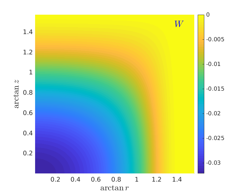
Figure 1: The function $W(r,z)$ that solves Eq. (2.46) for the semiclassical value of the size $\rho=\rho_{cl}$.

It is precisely the function $W(r,z)$ that will produce the leading-order term in the EDM of the nucleons. A numerical solution is shown in Fig. 1. The electromagnetic holographic current is given by

$$J^{\mu}_{\rm em}=\mathop{tr}\nolimits\left(J^{\mu}_{V}\tau^{3}\right)+\frac{1}{{N_{\rm c}}}\widehat{J}^{\mu}_{V},$$ (2.47)

where $\mathcal{J}^{\mu}_{V}$ is defined as

$$\mathcal{J}^{\mu}_{V}=-\kappa\left[k(z)\mathcal{F}^{\mu z}\right]^{+\infty}_{-\infty}.$$ (2.48)

Of this current we are interested in the component $J^{0}_{\rm em}$, since we want to compute the EDM of nucleons, defined by

$$\mathcal{D}_{\rm N}^{i}=e\int d^{3}x\,x^{i}\langle{\rm N}|J^{0}_{em}|{\rm N}\rangle=\mathcal{D}_{\rm N}\langle s|\sigma^{i}|s\rangle.$$ (2.49)

The EDM of the nucleon will consist of two terms with different symmetry properties under isospin transformations: we employ the following notation for these isovectorial and isoscalar parts:

$$\mathcal{D}_{\rm N}=d_{N}+\Delta_{N}\quad;\quad d_{n}=-d_{p}\quad;\quad\Delta_{n}=\Delta_{p}$$ (2.50)

We can immediately see that the Abelian part of Eq. (2.47) vanishes with the approximation employed, while the part constructed with the non-Abelian fields will contribute, having precisely a dipole structure (2.45). From this observation alone, we can already predict that the EDM $\mathcal{D}_{\rm N}$ will be proportional to the third component of the isospin operator $I_{3}$, and hence will be of equal magnitude and opposite sign for proton and neutron, thus only $d_{N}$ is nonvanishing at this order.

The computation confirms this, yielding the semiclassical ($Z=0$, $\rho=\rho_{\rm s.c.}$) results presented in [15]:

$$d_{n}=-d_{p}=0.78\times 10^{-16}\theta\text{ $e\cdot$cm}.$$ (2.51)

Effects of the nucleon wave function have been included in the results of [16] and turn out to be quantitatively important, but are not relevant for the purpose of this article since they do not change the isovectorial nature of $\mathcal{D}_{\rm N}$ at this level of approximation.

3 Perturbing the baryon at NLO

We will now take the perturbative approach to the next-to-leading order. The values of the parameters $\theta$ and $m/M_{\mathop{KK}\nolimits}$ will remain small, also in the phenomenologically relevant portion of the parameter space, so we will still keep terms which are first order with respect to them. On the other hand, higher orders in $\lambda^{-1},{N_{\rm c}}^{-1}$ will provide relevant corrections, in particular the leading contribution to the splitting of the magnitude of EDMs of nucleons.

For a field to give a nonvanishing EDM, it must be odd in the $\vec{x}$ coordinate: Since the holographic electromagnetic current is built from $\mathcal{F}_{z0}$, we are looking for perturbations in any field $\mathcal{A}$ that can result in perturbations $\delta\mathcal{A}_{z},\delta\mathcal{A}_{0}$ which are odd in $\vec{x}$. Since those fields are scalars under three-dimensional spatial rotations, the odd powers of $\vec{x}$ should come in scalar products (or combined with the antisymmetric tensor $\epsilon^{ijk}$) with other vectors: natural guesses are the angular velocity $\vec{\chi}$, the isospin $\vec{I}$ and the $SU(2)$ generators $\vec{\tau}$.

As shown by the results for the leading-order contribution to the NEDM, a $\delta A_{0,z}\propto\textbf{a}\vec{x}\cdot\vec{\tau}\textbf{a}^{-1}$ would not produce any splitting in the EDM magnitudes. More generally, it can be stated that the $SU(2)$ part alone of the current $J_{\mu}^{a=3}$ cannot produce a splitting of the EDMs due to its symmetry properties: Once evaluated on isospin eigenstates (i.e. the nucleons) it is bound to give results proportional to $I_{3}$, hence producing EDMs of equal magnitude (and opposite sign). The Abelian part of the current $\widehat{J}_{\mu}$ instead is an isoscalar: It acts blindly on nucleon states, so that also its action alone would produce EDMs of equal magnitude (and equal sign). When both terms are present, their combination is not isovectorial nor isoscalar, hence the EDMs will be split in magnitude.

Since the leading result for the nucleon EDM is given by the $SU(2)$ current, we now look for the leading $\theta$-dependent contribution to $\widehat{J}_{0}$. The only possible spatial vectors that can appear in $\widehat{J}_{0}$ are $\vec{\chi}$ and $\vec{x}$, hence we will look for perturbations in all the fields that can lead to a dipole structure

$$\widehat{J}_{0}\propto\mathcal{M}(r,z)(\vec{x}\cdot\vec{\chi}).$$ (3.1)

It is now clear in what sense we need to move to the next-to-leading order: since $\vec{\chi}$ is first order in time derivatives (which are to be regarded as ${N_{\rm c}}^{-1}$), we will now include such terms in the equations of motion and neglect higher-order terms. This means that we cannot drop time derivatives in the Yang-Mills part anymore, and we cannot approximate $\sin\varphi\sim 0$, but instead we need to include $\sin\varphi\sim\varphi$. Since we are stopping at the linear order in time derivatives, we can still approximate $\cos\varphi\sim 1$.

With this in mind, we can move to look at the equations of motion and seek for terms that could work as sources for the perturbations of order $m\theta$.

3.1 Relevant equations

We begin by recalling the equations in singular gauge, starting with the ones with explicit source terms coming from the Aharony-Kutasov action (i.e. the ones for $\mathcal{A}_{z}$). Up to first order in time derivatives and in the limit of small $\varphi$, they read

$$-\kappa k(z)\partial_{\mu}\widehat{F}^{z\mu}+\left(\mathop{CS}\nolimits\right) = cm\theta(\cos\alpha+1),$$

$$-\kappa k(z)D_{\nu}F^{z\nu}+\left(\mathop{CS}\nolimits\right) = -\frac{cm\theta}{2}\sin(\alpha)\varphi\,\textbf{a}\left(\hat{r}\cdot\vec{\tau}\right)\textbf{a}^{-1},$$ (3.2)

with

$$\varphi=-\frac{1}{2}\int^{+\infty}_{-\infty}dz\,\widehat{A}_{z}-\frac{\theta}{2}=\frac{{N_{\rm c}}}{64\pi\kappa}\frac{\rho^{2}}{(\rho^{2}+r^{2})^{3/2}}r\left(\hat{r}\cdot\vec{\chi}\right).$$ (3.3)

The other equations we are interested in are

$$-\kappa\left[h(z)D_{\nu}F^{i\nu}+D_{z}\left(k(z)F^{iz}\right)\right]+\left(\mathop{CS}\nolimits\right)=0,$$ (3.4)

$$-\kappa\left[h(z)\partial_{\nu}\widehat{F}^{0\nu}+\partial_{z}\left(k(z)\widehat{F}^{0z}\right)\right]-\frac{{N_{\rm c}}}{32\pi^{2}}\epsilon^{ijk}\left(F^{a}_{ij}F^{a}_{kz}+\widehat{F}_{ij}\widehat{F}_{kz}\right)=0.$$ (3.5)

The current $\widehat{J}_{0}$ we are interested in, is built from the field strength $\widehat{F}_{z0}$: still, the $\delta\widehat{A}_{z}$ field is suppressed with a time derivative, and also cannot acquire both a factor $\vec{\chi}$ and $\theta$ as can be argued from Eq. (3.1). The only perturbation that will directly enter the current is then $\delta\widehat{A}_{0}$, but we will keep the leading order solution for $\delta\widehat{A}_{z}$ given by Eq. (2.37).

As in Ref. [16], the Chern-Simons term will act as a source for this perturbation: the Abelian part of the Chern-Simons term in Eq. (3.5) reads

$$-\frac{{N_{\rm c}}}{32\pi^{2}}\epsilon^{ijk}\widehat{F}_{ij}\delta\widehat{F}_{kz}=\frac{{N_{\rm c}}}{16\pi^{2}}\frac{\rho^{2}}{(\xi^{2}+\rho^{2})^{2}}\frac{1}{r}\partial_{r}\delta\widehat{A}_{z}\left(\vec{x}\cdot\vec{\chi}\right).$$ (3.6)

Hence it is linear both in $\theta$ and $\vec{\chi}$ as desired.

However, at the same order, new sources may appear from the non-Abelian fields in the same Chern-Simons term: since the unperturbed field strength $F_{MN}$ does not contain neither $\vec{\chi}$ nor $\theta$, the perturbed $\delta A_{M}$ can only contribute if they are of order $\theta\vec{\chi}$ themselves. In the next section, we show how Eqs. (3.4) and (3.2) precisely contain sources of that order and must then be solved before moving to perturb Eq. (3.5).

3.2 Sources for $\delta A_{M}$

The possible source terms come from two parts of the equations: the perturbed Yang-Mills terms containing $\delta A_{0}$, and the Aharony-Kutasov term (since the function $\varphi$ contains $\vec{\chi}$). We will compute the Yang-Mills part in regular gauge for the sake of simplicity and for avoiding possible singularities in the numerical integration that will follow.

The perturbation $\delta A_{0}$ was obtained in Refs. [15, 16] in singular gauge, but it is simple to bring it back to the regular one, since the transformation acts on $\delta A_{0}$ as:

$$\delta A_{0}^{\rm(reg)}=Vg\,\textbf{a}^{-1}\delta A_{0}^{\rm(sing)}\textbf{a}\,g^{-1}V^{-1}=W(r,z)V\left(\hat{r}\cdot\vec{\tau}\right)V^{-1}.$$ (3.7)

The field $\delta A^{0}$ (2.45) is already of the order of $\theta$, and appears in Eqs. (3.2) and (3.4) with time derivatives, that will act on the functions $V,V^{-1}$ to generate $\Phi(x,z)$.

We will not follow the usual approach of solving first the static equations and then implementing time dependence modifying the static solution: We already know that we want to keep time derivatives up to first order, so we use the following Ansatz for the time dependence of the perturbed non-Abelian fields

$$\delta A(x,z,t)\equiv V\delta\widetilde{A}(x,z,\vec{\chi})V^{-1}.$$ (3.8)

The field $\delta A_{0}$ also shares this very same form if we consider $\delta\widetilde{A}_{0}=W(\vec{x}\cdot\vec{\chi})$.

The unperturbed fields are instead of the form

$$A(x,z,t)\equiv VA^{\rm cl}_{M}V^{-1}-iV\partial_{M}V^{-1}.$$ (3.9)

With these choices, the functions $V,V^{-1}$ can be factorized out respectively on the left and the right of the full perturbed Yang-Mills term as follows:

$$-\kappa k(z)V\left\{D_{j}^{\rm cl}\delta\widetilde{F}^{zj}+i\left[\delta\widetilde{A}_{j},F_{\rm cl}^{zj}\right]+i\left[\Phi,\partial_{z}\delta\widetilde{A}^{0}\right]\right.$$

$$\left.\quad-\left[\Phi,\left[A_{z}^{\rm cl},\delta\widetilde{A}^{0}\right]\right]+i\left[\delta\widetilde{A}_{0},F_{\rm cl}^{z0}\right]\right\}V^{-1}=(\text{AK term})^{\rm reg},$$ (3.10)

$$-\kappa h(z)V\left\{D_{j}^{\rm cl}\delta\widetilde{F}^{ij}+i\left[\delta\widetilde{A}_{j},F_{\rm cl}^{ij}\right]\right\}V^{-1}$$

$$\quad-\kappa V\left\{k(z)D_{z}^{\rm cl}\delta\widetilde{F}^{iz}+2z\delta\widetilde{F}^{iz}+k(z)i\left[\delta\widetilde{A}_{z},F^{iz}_{\rm cl}\right]\right\}V^{-1}$$

$$\quad-\kappa h(z)V\left\{i\left[\Phi,\partial_{i}\delta\widetilde{A}^{0}\right]-\left[\Phi,\left[A_{i}^{\rm cl},\delta\widetilde{A}^{0}\right]\right]+i\left[\delta\widetilde{A}_{0},F_{\rm cl}^{i0}\right]\right\}V^{-1}=0,$$ (3.11)

where we have neglected second-order time derivatives and made use of Eqs. (2.12) and (2.13). We do not need the explicit expression of the Aharony-Kutasov term in this gauge. It is evident that the last row of every equation is now a source term for the new perturbations $\delta\widetilde{A}_{M}$: However, cast this way, the equations are hard to solve, since we would need the full knowledge of the function $V(x,z,t)$. To overcome this problem we now transform the gauge back to singular gauge: the Yang-Mills term transforms covariantly, so it is simply obtained by the substitution $V\rightarrow\textbf{a}\,g^{-1}$. In singular gauge, we already computed the Aharony-Kutasov term, so we can restore its explicit form. Putting all the pieces together, we finally obtain the following set of equations:

$$\textbf{a}\,g^{-1}\left\{D_{j}^{\rm cl}\delta\widetilde{F}^{zj}+i\left[\delta\widetilde{A}_{j},F_{\rm cl}^{zj}\right]\right.$$

$$\quad\left.+i\left[\Phi,\partial_{z}\delta\widetilde{A}^{0}\right]-\left[\Phi,\left[A_{z}^{\rm cl},\delta\widetilde{A}^{0}\right]\right]+i\left[\delta\widetilde{A}_{0},F_{\rm cl}^{z0}\right]\right\}g\,\textbf{a}^{-1}$$

$$\quad-\textbf{a}\left[\frac{{N_{\rm c}}cm\theta}{128\pi\kappa^{2}}\frac{\rho^{2}}{(\rho^{2}+r^{2})^{3/2}}\frac{r}{k(z)}\sin\alpha\left(\hat{r}\cdot\vec{\chi}\right)\left(\hat{r}\cdot\vec{\tau}\right)\right]\textbf{a}^{-1}=0,$$ (3.12)

$$h(z)\,\textbf{a}\,g^{-1}\left\{D_{j}^{\rm cl}\delta\widetilde{F}^{ij}+i\left[\delta\widetilde{A}_{j},F_{\rm cl}^{ij}\right]\right\}g\,\textbf{a}^{-1}$$

$$\quad+\textbf{a}\,g^{-1}\left\{k(z)D_{z}^{\rm cl}\delta\widetilde{F}^{iz}+2z\delta\widetilde{F}^{iz}+k(z)i\left[\delta\widetilde{A}_{z},F^{iz}_{\rm cl}\right]\right\}g\,\textbf{a}^{-1}$$

$$\quad+h(z)\,\textbf{a}\,g^{-1}\left\{i\left[\Phi,\partial_{i}\delta\widetilde{A}^{0}\right]-\left[\Phi,\left[A_{i}^{\rm cl},\delta\widetilde{A}^{0}\right]\right]+i\left[\delta\widetilde{A}_{0},F_{\rm cl}^{i0}\right]\right\}g\,\textbf{a}^{-1}=0.$$ (3.13)

As can be seen, the last two rows of Eq. (3.12) and the last row of Eq. (3.13) are the source terms we were looking for: we now only need to factorize away the $\textbf{a},\textbf{a}^{-1}$ on each side of the equations, and exploit the fact that $g^{-1}\left(\hat{r}\cdot\vec{\tau}\right)g=g\left(\hat{r}\cdot\vec{\tau}\right)g^{-1}=\left(\hat{r}\cdot\vec{\tau}\right)$, to finally obtain our set of equations to solve

$$\left\{D_{j}^{\rm cl}\delta\widetilde{F}^{zj}+i\left[\delta\widetilde{A}_{j},F_{\rm cl}^{zj}\right]\right.$$

$$\quad\left.+i\left[\Phi,\partial_{z}\delta\widetilde{A}^{0}\right]-\left[\Phi,\left[A_{z}^{\rm cl},\delta\widetilde{A}^{0}\right]\right]+i\left[\delta\widetilde{A}_{0},F_{\rm cl}^{z0}\right]\right\}$$

$$\quad-\frac{{N_{\rm c}}cm\theta}{128\pi\kappa^{2}}\frac{\rho^{2}}{(\rho^{2}+r^{2})^{3/2}}\frac{r}{k(z)}\sin\alpha\left(\hat{r}\cdot\vec{\chi}\right)\left(\hat{r}\cdot\vec{\tau}\right)=0,$$ (3.14)

$$h(z)\left\{D_{j}^{\rm cl}\delta\widetilde{F}^{ij}+i\left[\delta\widetilde{A}_{j},F_{\rm cl}^{ij}\right]\right\}$$

$$\quad+\left\{k(z)D_{z}^{\rm cl}\delta\widetilde{F}^{iz}+2z\delta\widetilde{F}^{iz}+k(z)i\left[\delta\widetilde{A}_{z},F^{iz}_{\rm cl}\right]\right\}$$

$$\quad+h(z)\left\{i\left[\Phi,\partial_{i}\delta\widetilde{A}^{0}\right]-\left[\Phi,\left[A_{i}^{\rm cl},\delta\widetilde{A}^{0}\right]\right]+i\left[\delta\widetilde{A}_{0},F_{\rm cl}^{i0}\right]\right\}=0.$$ (3.15)

3.3 The Ansatz

We now want to solve the Eqs. (3.14) and (3.15): doing so is not an easy task since they are actually twelve coupled differential equations in four variables. Luckily enough, symmetry can be exploited to construct suitable Ansätze for the fields $\delta\widetilde{A}_{M}$: First of all, we note that three-dimensional radial symmetry of each field is only broken by the presence of the vectors $\vec{\chi}$ and $\vec{\tau}$. This means we can construct every structure that combines $\vec{\chi},\vec{\tau}$ and $\vec{x}$, and multiply each one of them by a function of $(r,z)$.

$$\delta\widetilde{A}_{z}\equiv K\left\{\beta(r,z)\left(\hat{r}\cdot\vec{\chi}\right)\left(\hat{r}\cdot\vec{\tau}\right)+\gamma(r,z)\left(\vec{\chi}\cdot\vec{\tau}\right)+\delta(r,z)\epsilon^{abc}\chi^{a}\hat{r}^{b}\tau^{c}\right\},$$ (3.16)

$$\delta\widetilde{A}_{i}\equiv K \Big{\{} B(r,z)\;\chi^{i}\left(\hat{r}\cdot\vec{\tau}\right)$$ (3.17)

$$+ C(r,z)\left(\hat{r}\cdot\vec{\chi}\right)\tau^{i}$$

$$+ D(r,z)\;\hat{r}^{i}\left(\vec{\chi}\cdot\vec{\tau}\right)$$

$$+ E(r,z)\;\epsilon^{iab}\chi^{a}\tau^{b}$$

$$+ F(r,z)\;\hat{r}^{i}\left(\hat{r}\cdot\vec{\chi}\right)\left(\hat{r}\cdot\vec{\tau}\right)$$

$$+ G(r,z)\;\hat{r}^{i}\epsilon^{abc}\chi^{a}\hat{r}^{b}\tau^{c}$$

$$+ H(r,z)\;\epsilon^{iab}\chi^{a}\hat{r}^{b}\left(\hat{r}\cdot\vec{\tau}\right)$$

$$+ I(r,z)\left(\hat{r}\cdot\vec{\chi}\right)\epsilon^{iab}\hat{r}^{a}\tau^{b}\Big{\}}.$$

We choose to use unit vectors $\hat{r}$ instead of $\vec{x}$. With this choice it will be easier to impose regularity of the fields at $r=0$, which will translate into simple Neumann conditions for the radial functions (exploiting $\partial_{r}\hat{r}=0$), and also every function will now have the same length dimension, regardless of how many coordinate vectors enter the respective group structure.

The complete set of eleven equations (with the corresponding boundary conditions) originating from this Ansatz plugged into Eqs. (3.14) and (3.15) is given in Appendix A. Since one of the fields that act as a source in this case is given by Eq. (2.45), we also choose the overall constant (factorized away in the equations in Appendix A) to be

$$K\equiv\frac{27\pi cm\theta}{\lambda\kappa}=\frac{{N_{\rm c}}cm\theta}{8\pi^{2}\kappa^{2}}.$$ (3.18)

The Ansatz for the field $\delta\widehat{A}^{0}$ is easier since now there is no group structure: the only possibility is

$$\delta\widehat{A}^{0}\equiv\Upsilon\mathcal{M}(r,z)\left(\hat{r}\cdot\vec{\chi}\right),$$ (3.19)

and since the perturbed fields $\delta\widetilde{A}_{M}$ appear as sources in Eq. (3.5) via the Chern-Simons term, we choose the overall constant $\Upsilon$ to be

$$\Upsilon\equiv\frac{{N_{\rm c}}K}{32\pi^{2}\kappa}=\frac{{N_{\rm c}}^{2}cm\theta}{256\pi^{4}\kappa^{3}}.$$ (3.20)

With all these choices, the resulting equation for $\mathcal{M}$ obtained by plugging Eqs. (3.17), (3.16), (2.37) and (3.19) into Eq. (3.5) reads

$$-h(z)\left(\mathcal{M}^{\prime\prime}+\frac{2}{r}\mathcal{M}^{\prime}-\frac{2}{r^{2}}\mathcal{M}\right)-2z\dot{\mathcal{M}}-k(z)\ddot{\mathcal{M}}$$

$$\quad+\frac{16\rho^{2}}{(\xi^{2}+\rho^{2})^{2}}\left(2E^{\prime}+\frac{2}{r}G-2H+2I^{\prime}+\frac{4}{r}I+\beta^{\prime}\right.$$

$$\phantom{\quad+\frac{16\rho^{2}}{(\xi^{2}+\rho^{2})^{2}}\bigg{(}}\left.+\frac{2}{r}\beta+\gamma^{\prime}-\dot{B}-3\dot{C}-\dot{D}-\dot{F}-\frac{1}{8}\frac{u^{\prime}}{k(z)}\right)$$

$$\quad+\frac{64\rho^{2}}{(\xi^{2}+\rho^{2})^{3}}\left(zB+3zC+zD-2rE-2rI-r\beta-r\gamma\right)=0.$$ (3.21)

Consistency requires that all the perturbations we turned on, do not change the baryonic number of the soliton solution. This is trivially guaranteed by the dipole structure of the perturbation: the baryon number density is given by the isoscalar charge density as

$$J^{0}_{B}\equiv-\frac{2}{{N_{\rm c}}}\kappa\left[k(z)\widehat{F}^{0z}\right]^{z=+\infty}_{z=-\infty}$$ (3.22)

so its perturbation amounts to:

$$\delta J^{0}_{B}=\frac{2}{{N_{\rm c}}}\kappa\left[k(z)\partial_{z}\delta\widehat{A}^{0}\right]^{z=+\infty}_{z=-\infty}=\frac{2}{{N_{\rm c}}}\kappa\Upsilon\left[k(z)\partial_{z}\mathcal{M}\left(\hat{r}\cdot\vec{\chi}\right)\right]^{z=+\infty}_{z=-\infty}$$ (3.23)

which is odd in $\vec{x}$ and thus vanishes upon integration over the solid angle.

4 Neutron-proton EDM splitting

We now move to compute the splitting in the EDM magnitude of the nucleons: we recall the definition of the electric dipole moment for a baryon:

$$\mathcal{D}^{i}_{B}=e\int d^{3}x\,x^{i}\langle B,s|J^{0}_{\rm em}|B,s\rangle=\mathcal{D}_{B}\langle s|\sigma^{i}|s\rangle,$$ (4.1)

where $|B,s\rangle$ is a baryonic state and the last equality defines $\mathcal{D}_{B}$ requiring the EDM vector to be proportional to the spin (since it is the only physical vector intrinsic to the baryon).

We call the subleading correction we are about to compute $\Delta_{\rm N}^{i}$ following (2.50), since it will correspond to the isoscalar contribution. Of course it will still obey the relation

$$\Delta_{\rm N}^{i}=\Delta_{\rm N}\langle s|\sigma^{i}|s\rangle.$$ (4.2)

Our aim now is to compute the value of $\Delta_{\rm N}$. As we already mentioned, only the Abelian part of the current (2.47) will give contributions to it, so for our purpose, the perturbed current effectively reads

$$\delta J^{0}_{\rm em}=-\kappa\left[k(z)\delta\widehat{F}^{0z}\right]^{+\infty}_{-\infty}=\frac{\kappa}{{N_{\rm c}}}\left[k(z)\partial_{z}\delta\widehat{A}^{0}\right]^{+\infty}_{-\infty}=\Upsilon\frac{\kappa}{{N_{\rm c}}}\left[k(z)\partial_{z}\mathcal{M}\right]^{+\infty}_{-\infty}\left(\hat{r}\cdot\vec{\chi}\right).$$ (4.3)

Plugging this expression into the EDM formula yields:

$$\Delta_{\rm N}^{i}=e\Upsilon\frac{\kappa}{{N_{\rm c}}}\int d^{3}x\,x^{i}\langle{\rm N}|\left[k(z)\partial_{z}\mathcal{M}\right]^{+\infty}_{-\infty}\left(\hat{r}\cdot\vec{\chi}\right)|{\rm N}\rangle.$$ (4.4)

Since we approximate the massive moduli by their classical values, we can just keep the angular velocity in the expectation value. We further switch to spherical coordinates and integrate over $d\Omega$:

$$\Delta_{\rm N}^{i}=e\Upsilon\frac{\kappa}{{N_{\rm c}}}\frac{4\pi}{3}\int dr\,r^{3}\left[k(z)\partial_{z}\mathcal{M}\right]^{+\infty}_{-\infty}\langle{\rm N}|\chi^{i}|{\rm N}\rangle.$$ (4.5)

Now, making use of (2.20) (setting again $\rho=\rho_{\rm cl}$) and writing $J^{k}\equiv\frac{1}{2}\sigma^{k}$ we finally obtain:

$$\Delta_{\rm N}^{i}=\frac{ecm\theta}{192\pi^{3}\kappa^{2}}\sqrt{\frac{5}{6}}\int dr\,r^{3}\left[k(z)\partial_{z}\mathcal{M}\right]^{+\infty}_{-\infty}\langle{\rm N}|\sigma^{i}|{\rm N}\rangle.$$ (4.6)

To make a prediction for $\Delta_{\rm N}$ we use, other than ${N_{\rm c}}=3$, the most common parameter choices for the Sakai-Sugimoto model, i.e.:

$$\kappa=0.00745\quad;\quad M_{\mathop{KK}\nolimits}=949\;\text{MeV}\quad;\quad m=2.92\;\text{MeV}$$ (4.7)

The quark mass $m$ is chosen such that it correctly reproduces $m_{\pi}=135\;$MeV in the GMOR relation $4cm=f_{\pi}^{2}m_{\pi}^{2}$, and it turns out being a physically reasonable value that lies in between those of the up and down quark masses. The pion decay constant is given in Ref. [13] in terms of $\kappa$:

$$f_{\pi}^{2}=4\frac{\kappa}{\pi}.$$ (4.8)

With these choices, and restoring factors of $M_{\mathop{KK}\nolimits}$ by simple dimensional analysis, our prediction is

$$\Delta_{\rm N}=-4.6\times 10^{-17}\theta\text{ $e\cdot$cm}$$ (4.9)

It is possible to repeat the computation for different values of $\lambda$ in order to extract the scaling of the EDM in the large $\lambda$ limit. Of course there is a limitation to how large we can take $\lambda$, since for $\lambda\rightarrow\infty$ the instanton becomes pointlike and the precision of the numerical solution is lost. Nevertheless, we manage to reach $\lambda=10^{3.5}$ while keeping a trustable solution.

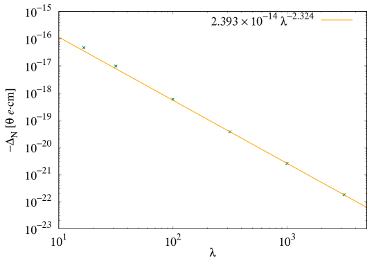
Figure 2: The logarithmic plot of $\Delta_{\rm N}$ for increasing values of $\lambda$, starting with the phenomenological one. As can be seen, the $\lambda$ dependency tends to a definite power law in the large $\lambda$ limit.

The result we obtain for the scaling at large $\lambda$ is

$$\Delta_{\rm N}\sim-2.393\times 10^{-14}\lambda^{-2.324}\theta\text{ $e\cdot$cm},$$ (4.10)

see Fig. 2. Note that this contribution is consistently suppressed with respect to the isovectorial one, that scales as $\lambda^{-2}$ [15], but not strongly, which allows to obtain the correct order of magnitude with extrapolation to phenomenological $\lambda$.

5 From the nucleons to the deuteron

Computing the EDM of the deuteron requires us to have $B=2$ quantum states: Of course we need in particular the ground state of that topological sector. There are at least two different consistent ways of obtaining such state, following from the non-commutativity of the two large-${N_{\rm c}}$ and large-$\lambda$ limits. Nonetheless, at leading order, our computation is not dependent on such details, so it yields the same result no matter how we build the Sakai-Sugimoto deuteron state as long as it has the correct quantum numbers.

A few considerations on such numbers: we know from phenomenology that the ground state is in the isospin singlet, spin triplet configuration $(I=0,J=1)$, and its orbital wave function is mostly composed of the $L=0$ state, with a small part of the $L=2$ one. We will assume $L=0$ from now on, since from the holographic point of view the $L=2$ component has to be suppressed by powers of $\lambda^{-1}$: this can simply be understood by considering that the $L=2$ component is geometrically realized by the two nucleons spinning around an axis orthogonal to their separation. In this configuration, we can estimate the moment of inertia for rotations around this axis as $2M_{B}R^{2}$: The separation between the nucleons’ cores is of order $R\sim\mathcal{O}(1)$, as verified in Ref. [31], while the leading order of the baryon mass is given by $M_{B}=8\pi^{2}\kappa$. Hence it is of order $\lambda$ and so is the moment of inertia.

On the other hand, the $L=0$ configuration involves no other angular momentum than the spin of the nucleons, as it can be thought of as the two spins lying along the separation between the nucleons and pointing in the same direction. Thus the moment of inertia for this angular momentum is given by the sum of the ones of the single solitons, each amounting to $4\pi^{2}\kappa\rho^{2}$. Since the classical value of the size is given by Eq. (2.10), this moment of inertia does not scale with $\lambda$, hence the $L=0$ component dominates the orbital wave function once the large-$\lambda$ limit is taken.

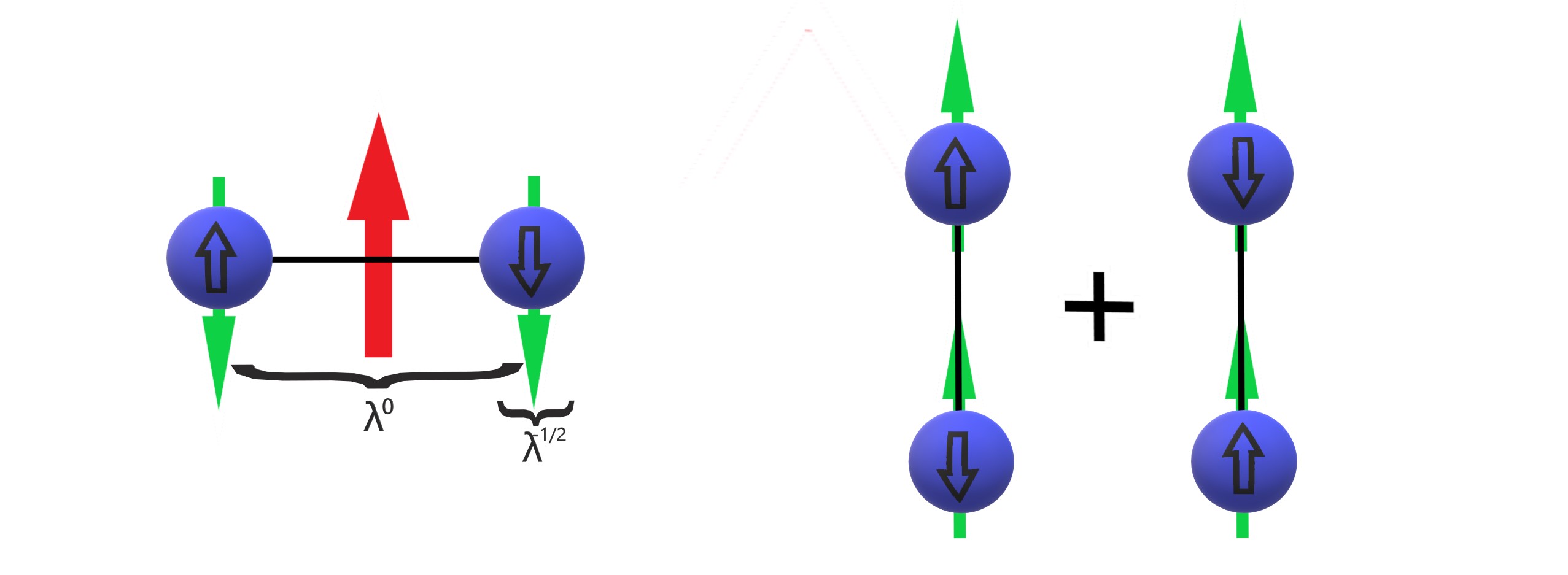
Figure 3: Configuration of the two solitons in the $L=2$ (left) and $L=0$ (right) sectors: The arrows denote the directions of spatial angular momentum (red), single soliton spin (green) and single soliton iso-orientation (on the soliton). The size of each soliton is of order $\lambda^{-1/2}$, while the separation between them is of order $\lambda^{0}$. In the quantum ground state, each soliton is in a superposition of opposite isospin direction.

.

5.1 Deuteron EDM

The deuteron is shaped by placing two solitons at the distance $R$ that minimizes the nucleon-nucleon potential, and assigning to each of them the $SU(2)$ orientation described respectively by the matrices $B,C$:

$$\mathcal{A}=B\mathcal{A}^{\rm cl}_{(1)}\left(\vec{x}+\frac{\vec{R}}{2},z\right)B^{\dagger}+C\mathcal{A}^{\rm cl}_{(2)}\left(\vec{x}-\frac{\vec{R}}{2},z\right)C^{\dagger}.$$ (5.1)

The two approaches in the construction of the deuteron treat the moduli of $SU(2)$ differently: The solitons are either treated as spinning independently, or as having a locked relative orientation. Since we are interested in the Abelian part of the current, such details will not play any role, as the $SU(2)$ moduli will only enter the computation via the total angular momentum. The full EDM can be computed as two separate contributions:

$$\mathcal{D}_{\rm D}^{i}=e\int d^{3}x\left(x^{i}-x_{0}^{i}\right)\langle{\rm D},s|\mathop{tr}\nolimits\left(\delta J^{0}_{V}\tau^{3}\right)+\frac{1}{{N_{\rm c}}}\delta\widehat{J}^{0}_{V}|{\rm D},s\rangle=\left(d_{\rm D}+\Delta_{\rm D}\right)\langle j|\sigma^{i}|j\rangle.$$ (5.2)

In the following sections we will show that, in both approaches to the deuteron, we obtain the simple results

$$d_{\rm D}=0,$$ (5.3)

$$\Delta_{\rm D}=2\Delta_{\rm N}.$$ (5.4)

The $SU(2)$ part of the electromagnetic charge density comes in the form

$$\mathop{tr}\nolimits\left(\delta J^{0}_{V}\tau^{3}\right)=K\kappa\left[k(z)\partial_{z}W^{(1)}\hat{r}_{1}\cdot\mathop{tr}\nolimits\left(B\vec{\tau}B^{\dagger}\tau^{3}\right)+k(z)\partial_{z}W^{(2)}\hat{r}_{2}\cdot\left(\ C\vec{\tau}C^{\dagger}\tau^{3}\right)\right]^{+\infty}_{-\infty}.$$ (5.5)

The complete field strength $\delta F^{0z}$ would also include a term of the form $[\delta A^{0}_{(1)}$+$\delta A^{0}_{(2)}$, $A^{z}_{(1)}$ + $A^{z}_{(2)}]$ but it can easily be checked to vanish, since $\delta A^{0}$ and $A^{z}$ share the same group structure $f(r,z)\vec{x}\cdot\textbf{a}\vec{\tau}\textbf{a}^{-1}$.

The new $U(1)$ part reads

$$\delta\widehat{J}^{0}_{\rm em}\equiv\frac{1}{{N_{\rm c}}}\delta\widehat{J}^{0}_{V}=\Upsilon\frac{\kappa}{{N_{\rm c}}}\left[k(z)\partial_{z}\mathcal{M}^{(1)}(\hat{r}_{1}\cdot\vec{\chi}^{(1)})+k(z)\partial_{z}\mathcal{M}^{(2)}(\hat{r}_{2}\cdot\vec{\chi}^{(2)})\right]^{+\infty}_{-\infty}.$$ (5.6)

In both equations, we have defined $\hat{r}_{1}=\frac{\vec{x}+\frac{\vec{R}}{2}}{|\vec{x}+\frac{\vec{R}}{2}|}$ and $\hat{r}_{2}=\frac{\vec{x}-\frac{\vec{R}}{2}}{|\vec{x}-\frac{\vec{R}}{2}|}$.

5.2 Approach 1

In this approach, given in Ref. [31], the deuteron state $|{\rm D}\rangle$ is obtained by quantizing the $B=2$ zero modes manifold: the massless $SU(2)\times SU(2)$ moduli corresponding to global iso- and spatial rotations are given by the matrices $U\equiv u_{4}+iu_{k}\tau^{k}$ and $E\equiv e_{4}+ie_{k}\tau^{k}$. They can be related to the single soliton moduli $B$ and $C$ via the embedding law:

$$B=UE^{\dagger},$$ (5.7)

$$C=iU\tau^{3}E^{\dagger},$$ (5.8)

where the factor $i\tau^{3}$ in Eq. (5.8) is present because the relative orientation of the nucleons is not a massless modulus: the nucleon-nucleon potential is found to be a function of the moduli $(\rho_{1},\rho_{2},Z_{1},Z_{2},B^{\dagger}C)$, hence the $i\tau^{3}$ factor selects the attractive channel, performing a relative rotation in isospin space of $\pi$ around an axis orthogonal to the separation between nucleons.

The found deuteron state can be written in terms of the global moduli $e_{I}$:

$$\langle e_{I},u_{I}|{\rm D}\rangle=\frac{1}{\pi^{2}}\left(2\left(e_{3}^{2}+e_{4}^{2}\right)-1\right),$$ (5.9)

but it is more useful to write it using the single soliton moduli $b_{I},c_{I}$:

$$\langle b_{I},c_{I}|{\rm D}\rangle=\frac{1}{\pi^{2}}\left(b_{4}c_{3}-b_{3}c_{4}+b_{1}c_{2}-b_{2}c_{1}\right).$$ (5.10)

As a first step, we show that the dipole moment of Eq. (5.5) vanishes on the deuteron state. We have to compute the quantity

$$d_{\rm D}^{i}=eK\kappa\langle{\rm D}|\int d^{3}x\,x^{i}\left[k(z)\left(\partial_{z}W^{(1)}\hat{r}_{1}\cdot\mathop{tr}\nolimits\left(B\vec{\tau}B^{\dagger}\tau^{3}\right)+\partial_{z}{W}^{(2)}\hat{r}_{2}\cdot\left(C\vec{\tau}C^{\dagger}\tau^{3}\right)\right)\right]^{+\infty}_{-\infty}|{\rm D}\rangle.$$

To begin with, we note that the two integrals of $\dot{W}^{(1)}$ and $\dot{W}^{(2)}$ give the same result, since it is sufficient to perform separately the change of variables $\vec{x}\rightarrow\vec{x}\mp\frac{\vec{r}}{2}$ to make them explicitly the same integral. Then we note that Eq. (5.10) is antisymmetric under the exchange of $b_{I}$ with $c_{I}$. Thus to obtain the full result, we only need to compute

$$\langle{\rm D}|\mathop{tr}\nolimits\left(B\tau^{i}B^{\dagger}\tau^{3}\right)|{\rm D}\rangle,$$ (5.11)

which turns out to vanish for every $i=1,2,3$. Hence we conclude that the $SU(2)$ part of the current does not contribute to the deuteron EDM: this is in line with what we expected, a result proportional to the total isospin, which is zero for the deuteron. In principle one could expect the contributions of the two nucleons to cancel each other, as the classical picture of a neutron with $I_{3}=-\frac{1}{2}$ and a proton with $I_{3}=+\frac{1}{2}$ would suggest: the fact that each contribution vanishes on its own instead is due to the fact that the quantum state Eq. (5.10) does not assign a definite $I_{3}$ to each nucleon, but both are in an equally probable superposition of neutron and proton states (as shown in fig. 3), hence the average $I_{3}$ of each soliton vanishes.

Now we turn to the computation of $\Delta_{\rm D}^{i}$:

$$\Delta_{\rm D}^{i}=e\Upsilon\frac{\kappa}{{N_{\rm c}}}\langle{\rm D}|\int d^{3}x\,x^{i}\left[k(z)\partial_{z}\mathcal{M}^{(1)}(\hat{r}_{1}\cdot\vec{\chi}^{(1)})+k(z)\partial_{z}\mathcal{M}^{(2)}(\hat{r}_{2}\cdot\vec{\chi}^{(2)})\right]^{+\infty}_{-\infty}|{\rm D}\rangle.$$ (5.12)

As before, the integrals can be evaluated separately, and each of them reproduce the result of Eq. (4.5), so we are left with

$$\Delta_{\rm D}^{i}=e\Upsilon\frac{\kappa}{{N_{\rm c}}}\frac{4\pi}{3}\int dr\,r^{3}\left[k(z)\dot{\mathcal{M}}\right]^{+\infty}_{-\infty}\langle{\rm D}|\chi^{i}_{(1)}+\chi^{i}_{(2)}|{\rm D}\rangle.$$ (5.13)

By making use of (2.20) we trade the angular velocities for the angular momenta:

$$\Delta_{\rm D}^{i}=\frac{e\Upsilon}{3\pi\rho^{2}{N_{\rm c}}}\int dr\,r^{3}\left[k(z)\partial_{z}\mathcal{M}\right]^{+\infty}_{-\infty}\langle{\rm D}|J^{i}_{(1)}+J^{i}_{(2)}|{\rm D}\rangle.$$ (5.14)

The last step is to use the fact that $L=0$, so effectively $J_{\rm D}^{i}=J_{(1)}^{i}+J_{(2)}^{i}$, and thus we obtain the aforementioned result

$$\Delta_{\rm D}^{i}=\frac{ecm\theta}{96\pi^{3}\kappa^{2}}\sqrt{\frac{5}{6}}\int dr\,r^{3}\left[k(z)\partial_{z}\mathcal{M}\right]^{+\infty}_{-\infty}\langle{\rm D}|J_{\rm D}^{i}|{\rm D}\rangle=2\Delta_{\rm N}\langle{\rm D}|J_{\rm D}^{i}|{\rm D}\rangle.$$ (5.15)

which is the full result for the EDM of the deuteron:

$$\mathcal{D}_{\rm D}=2\Delta_{\rm N}=-0.92\times 10^{-16}\theta\text{ $e\cdot$cm}$$ (5.16)

5.3 Approach 2

Another possible setup is the one adopted in Ref. [32]. Since the two solitons are placed at a distance much greater than their size, they can be treated as independent identical particles. Since each of them is quantized as a fermion, we can build the global wave function $|{\rm D}\rangle$ as an antisymmetric combination of the two single soliton states with $SU(2)$ quantum numbers $l=1$, $|{\rm N}\rangle=|l/2=\frac{1}{2},m_{s},m_{i}\rangle$. Antisymmetry in the $I_{3}$ quantum number leads us to

$$|{\rm D},m_{j}\rangle=\frac{1}{\sqrt{2}}\left(|{\rm p},m_{s}\rangle|{\rm n},m_{s}\rangle-|{\rm n},m_{s}\rangle|{\rm p},m_{s}\rangle\right),$$ (5.17)

with $m_{j}=2m_{s}$. This configuration still does not assign a definite third component of the isospin to any of the two solitons (it is still of the type illustrated on the right-hand side of Fig. 3), so the argument for the vanishing of $d_{\rm D}$ we used in the previous section is still valid here.

It is also still true that $J_{\rm D}^{i}=J_{(1)}^{i}+J_{(2)}^{i}$ so Eq. (5.16) also holds its validity.

6 Conclusion

Using the holographic model of Witten-Sakai-Sugimoto, we were able to extend the computation of the EDMs of baryons to the isoscalar part. It turns out to be of a comparable magnitude with the isovectorial one, once extrapolation to phenomenological values of the parameters of the model is performed, despite it being a subleading correction in $\lambda^{-1}$ and ${N_{\rm c}}^{-1}$. In particular, we observe the scalings $\Delta_{\rm N}/d_{N}\sim\mathcal{O}(\lambda^{-1}{N_{\rm c}}^{-2})$.

Using the deuteron description emerging from the same model and the results for the EDMs of nucleons, we were able to estimate the EDM of the deuteron bound state, obtaining a value close to the estimate given in Ref. [3]: even if this numerical closeness may be regarded as an accident, considering the many approximations implicit in our computations (and the lack of the inclusion of two-body contributions which are expected to give comparable EDMs), it is still remarkable that we obtain the correct order of magnitude and sign, despite this term being formally subleading in $\lambda$ and ${N_{\rm c}}$ before phenomenological extrapolation of the parameters. This can be ultimately traced back to the known fact that the perturbative regime in the Sakai-Sugimoto model is not well established at phenomenological values of the model parameters, especially for the baryonic sector. In this sense, it is clear that our result for the deuteron EDM can receive significant corrections at subsequent orders in this perturbative expansion (as happens explicitly for the single nucleons) and is thus to be regarded as order of magnitude estimates of the EDMs. While it is not really significant in this sense to change the estimates of the single nucleon EDMs previously obtained in Refs. [15] and [16], as the exact value can be further modified with higher order corrections, it is indeed relevant for the newly computed deuteron EDM, being the leading order and thus establishing the order of magnitude and sign for the quantity within this model. Moreover, we stress that unlike the single nucleon EDMs, the deuteron EDM receive corrections only from terms in the perturbative expansion that can contribute to the isoscalar charge density $\delta\widehat{J}^{0z}$: extending the mechanism that generates source terms for the perturbations from the mass term in the equations of motion, it is clear that the next contribution to the isoscalar current would arise at NNNLO, as the one at NNLO is isovectorial.

Two-body terms can be divided into two conceptually different classes: polarization terms ($\mathcal{D}_{\rm D}^{\rm(pol)}$) and exchange terms ($\mathcal{D}_{\rm D}^{\rm(exc)}$). The first ones account for P-wave components in the wave function of the deuteron, and pion-nucleon coupling $\bar{g}_{\pi NN}^{(1)}$. The second class arises from the exchange of currents between the nucleons, and can potentially receive contributions from both the isospin-preserving, CP-breaking pion-nucleon couplings $\bar{g}_{\pi NN}^{(0)}$ and $\bar{g}_{\pi{\rm NN}}^{(1)}$. The term that dominates, however, is expected to be the polarization one, and in the exchange term the bigger role is played by pieces proportional to $\bar{g}_{\pi NN}^{(1)}$. However, in the setup we employed, we only expect two-body contributions to arise from $\bar{g}_{\pi NN}^{(0)}$, since we did not include isospin-breaking terms in the quark mass matrix, we lose all the larger pieces of this two-body term.

To be fully self consistent we only need to account for the exchange term that picks up $\bar{g}_{\pi NN}^{(0)}$: Conceptually, one would need to perturb the full two-soliton configuration, and look for $\theta$-induced perturbations of the soliton tail. This looks like an overly-hard task, but it is reasonable to expect that such term is subleading in $\lambda^{-1}$, being the outcome of the perturbation of a solitonic tail (which can be regarded as a perturbation to the soliton core) induced by a perturbation of the cores (that is, the $\theta$-induced perturbations we found).

Appendix A Explicit equations of motion

Here we provide the equations of motion to be solved for every group structure of the Ansatz we employed. The function $W(r,z)$ is defined by Eq. (2.46). The functions $\beta,\gamma,\delta$ appear with only the first derivative with respect to $z$, while the functions $D,F,G$ appear with only the first derivative with respect to $r$. All the other functions appear with all the derivatives up to second order with respect to both coordinates. Note that every function has a definite parity under $z\rightarrow-z$, so the boundary condition at infinity for the $z$ coordinate can be imposed either at $z=+\infty$ or $z=-\infty$: The equations will take care of the behavior of the functions on the other side of the $z$ axis. The boundary conditions at $z=0$ can instead be guessed from the parity of each function: $\beta,\gamma,E,G,H,I$ are even, while $\delta,B,C,D,F$ are odd. The boundary conditions we impose are thus:

$$\beta^{\prime}(0,z)=\gamma^{\prime}(0,z)=\delta^{\prime}(0,z)=0,$$

$$\beta(+\infty,z)=\gamma(+\infty,z)=\delta(+\infty,z)=0,$$

$$\beta(r,\infty)=\gamma(r,\infty)=\delta(r,\infty)=0,$$

$$B^{\prime}(0,z)=C^{\prime}(0,z)=E^{\prime}(0,z)=H^{\prime}(0,z)=I^{\prime}(0,z)=0,$$

$$X(+\infty,z)=0,\quad\qquad\qquad\qquad{\rm for}\qquad X=B,\dots,I,$$

$$B(r,0)=C(r,0)=D(r,0)=F(r,0)=0,$$

$$\dot{E}(r,0)=\dot{G}(r,0)=\dot{H}(r,0)=\dot{I}(r,0)=0,$$

$$X(r,\infty)=0,\qquad\qquad\qquad\qquad{\rm for}\qquad X=B,\dots,I.$$ (A.1)

• $\left(\hat{r}\cdot\vec{\chi}\right)\left(\hat{r}\cdot\vec{\tau}\right)$

  $$\dot{B^{\prime}}-\frac{1}{r}\dot{B}+\dot{C^{\prime}}-\frac{1}{r}\dot{C}+\dot{F^{\prime}}+\frac{2}{r}\dot{F}-\beta^{\prime\prime}-\frac{2}{r}\beta^{\prime}+\frac{6}{r^{2}}\beta$$

  $$+\frac{2}{\xi^{2}+\rho^{2}}\left[r\dot{B}+2r\dot{C}+rE^{\prime}-rG^{\prime}+z\dot{G}-3G-z\dot{H}+2z\dot{I}-3I-6\beta-2z\delta^{\prime}+2\frac{z}{r}\delta\right]$$

  $$+\frac{4}{(\xi^{2}+\rho^{2})^{2}}\left[-2zrC-zrD+r^{2}E+(r^{2}-\rho^{2})G+\rho^{2}H+2(r^{2}-\rho^{2})I+2\xi^{2}\beta+r^{2}\gamma+zr\delta\right]$$

  $$+\frac{2r^{2}}{\xi^{2}+\rho^{2}}\left[z\dot{W}-\frac{\rho^{2}}{\xi^{2}+\rho^{2}}W\right]$$

  $$-\frac{\pi}{16}\frac{\rho^{2}}{(\rho^{2}+r^{2})^{3/2}}\frac{r}{k(z)}\sin\left(\frac{\pi}{\sqrt{1+\frac{\rho^{2}}{r^{2}}}}\right)=0,$$ (A.2)

• $\left(\vec{\chi}\cdot\vec{\tau}\right)$

  $$\frac{1}{r}\dot{B}+\frac{1}{r}\dot{C}+\dot{D^{\prime}}+\frac{2}{r}\dot{D}-\frac{2}{r^{2}}\beta-\gamma^{\prime\prime}-\frac{2}{r}\gamma^{\prime}$$

  $$+\frac{2}{\xi^{2}+\rho^{2}}\left[-r\dot{B}+2z\dot{E}-rE^{\prime}-2E-z\dot{G}+rG^{\prime}+3G+z\dot{H}+I+2\beta+2z\delta^{\prime}+2\frac{z}{r}\delta\right]$$

  $$+\frac{4}{(\xi^{2}+\rho^{2})^{2}}\left[(2z^{2}+r^{2})\gamma-zr\delta+zrD+(r^{2}-2\rho^{2})E+(\rho^{2}-r^{2})G-\rho^{2}H\right]$$

  $$+\frac{2r^{2}}{\xi^{2}+\rho^{2}}\left[-z\dot{W}+\frac{\rho^{2}}{\xi^{2}+\rho^{2}}W\right]=0,$$ (A.3)

• $\epsilon^{abc}\chi^{a}\hat{r}^{b}\tau^{c}$

  $$-\dot{E^{\prime}}+\dot{G^{\prime}}+\frac{2}{r}\dot{G}+\frac{1}{r}\dot{H}+\frac{1}{r}\dot{I}-\delta^{\prime\prime}-\frac{2}{r}\delta^{\prime}+\frac{2}{r^{2}}\delta$$

  $$+\frac{2}{\xi^{2}+\rho^{2}}\left[-z\dot{B}-C+z\dot{D}-rD^{\prime}-3D-r\dot{E}-r\dot{H}+2\frac{z}{r}\beta-2z\gamma^{\prime}-2\delta\right]$$

  $$+\frac{4}{(\xi^{2}+\rho^{2})^{2}}\left[\rho^{2}B+(r^{2}-\rho^{2})D-zrE+zrG+zr\gamma+(2z^{2}+r^{2})\delta\right]$$

  $$+\frac{r}{\xi^{2}+\rho^{2}}\left[-(z^{2}-r^{2})\dot{W}+\frac{2\rho^{2}}{\xi^{2}+\rho^{2}}zW\right]=0,$$ (A.4)

• $\chi^{i}\left(\hat{r}\cdot\vec{\tau}\right)$

  $$h(z)\left[-B^{\prime\prime}-\frac{1}{r}B^{\prime}+\frac{1}{r^{2}}B+\frac{1}{r}C^{\prime}-\frac{1}{r^{2}}C+\frac{1}{r}F^{\prime}\right]+k(z)\left[\frac{1}{r}\dot{\beta}-\ddot{B}\right]+2z\left[\frac{1}{r}\beta-\dot{B}\right]$$

  $$+\frac{2h(z)}{\xi^{2}+\rho^{2}}\left[-2B+C+rD^{\prime}+2D-zE^{\prime}+zG^{\prime}+\frac{z}{r}G+\frac{z}{r}I\right]$$

  $$+\frac{4h(z)}{(\xi^{2}+\rho^{2})^{2}}\left[\xi^{2}B+(\rho^{2}-r^{2})D+zrE-zrG\right]$$

  $$+\frac{2k(z)}{\xi^{2}+\rho^{2}}\left[z\dot{\delta}+\delta+r\dot{\gamma}\right]+\frac{4z}{\xi^{2}+\rho^{2}}\left[r\gamma+z\delta\right]$$

  $$+\frac{4k(z)}{(\xi^{2}+\rho^{2})^{2}}\left[-z^{2}\delta+\rho^{2}\delta-zr\gamma\right]$$

  $$+h(z)\frac{W}{(\xi^{2}+\rho^{2})^{2}}2zr\rho^{2}=0,$$ (A.5)

• $\left(\hat{r}\cdot\vec{\chi}\right)\tau^{i}$

  $$h(z)\left[+\frac{1}{r}B^{\prime}-\frac{1}{r^{2}}B-C^{\prime\prime}-\frac{1}{r}C^{\prime}+\frac{1}{r^{2}}C+\frac{1}{r}F^{\prime}\right]+k(z)\left[\frac{1}{r}\dot{\beta}-\ddot{C}\right]+2z\left[\frac{1}{r}\beta-\dot{C}\right]$$

  $$+\frac{2h(z)}{\xi^{2}+\rho^{2}}\left[-rB^{\prime}-B-rC^{\prime}-2C-rD^{\prime}-2D+2zE^{\prime}-rF^{\prime}-2F+\frac{z}{r}G-3\frac{z}{r}H+2zI^{\prime}+4\frac{z}{r}I\right]$$

  $$+\frac{4h(z)}{(\xi^{2}+\rho^{2})^{2}}\left[(\xi^{2}-\rho^{2})B+(4z^{2}+r^{2}-2\rho^{2})C+(\xi^{2}-\rho^{2})D-3zrE+(\xi^{2}-\rho^{2})F-3zrI\right]$$

  $$+\frac{2k(z)}{\xi^{2}+\rho^{2}}\left[-2r\dot{E}-2r\dot{I}-r\dot{\beta}-r\dot{\gamma}-\delta\right]+\frac{4z}{\xi^{2}+\rho^{2}}\left[-rE-rI-r\beta-r\gamma\right]$$

  $$+\frac{4k(z)}{(\xi^{2}+\rho^{2})^{2}}\left[r^{2}C+zrE+zrI\right]$$

  $$+h(z)\frac{W}{(\xi^{2}+\rho^{2})^{2}}2zr(\xi^{2}-\rho^{2})=0,$$ (A.6)

• $\hat{r}^{i}\left(\vec{\chi}\cdot\vec{\tau}\right)$

  $$h(z)\left[\frac{1}{r}B^{\prime}-\frac{1}{r^{2}}B+\frac{1}{r}C^{\prime}-\frac{1}{r^{2}}C-\frac{2}{r^{2}}F\right]+k(z)\left[\dot{\gamma^{\prime}}-\ddot{D}\right]+2z\left[\gamma^{\prime}-\dot{D}\right]$$

  $$+\frac{2h(z)}{\xi^{2}+\rho^{2}}\left[-rB^{\prime}+B+2C+zE^{\prime}+2F+zH^{\prime}+\frac{z}{r}H-\frac{z}{r}I\right]$$

  $$+\frac{4h(z)}{(\xi^{2}+\rho^{2})^{2}}\left[\rho^{2}B+\xi^{2}D\right]$$

  $$+\frac{2k(z)}{\xi^{2}+\rho^{2}}\left[2r\dot{E}-2r\dot{G}-z\dot{\delta}-\delta+r\delta^{\prime}\right]+\frac{4z}{\xi^{2}+\rho^{2}}\left[rE-rG-z\delta\right]$$

  $$+\frac{4k(z)}{(\xi^{2}+\rho^{2})^{2}}\left[r^{2}D-zrE+zrG+zr\gamma+(z^{2}-\rho^{2})\delta\right]$$

  $$+h(z)\left[-\frac{W^{\prime}}{\xi^{2}+\rho^{2}}2zr^{2}-\frac{W}{(\xi^{2}+\rho^{2})^{2}}2zr\xi^{2}\right]=0,$$ (A.7)

• $\epsilon^{iab}\chi^{a}\tau^{b}$

  $$h(z)\left[-E^{\prime\prime}-\frac{1}{r}E^{\prime}-\frac{1}{r}G^{\prime}-\frac{3}{r^{2}}H-\frac{3}{r^{2}}I\right]+k(z)\left[-\frac{1}{r}\dot{\delta}-\ddot{E}\right]+2z\left[-\frac{1}{r}\delta-\dot{E}\right]$$

  $$+\frac{2h(z)}{\xi^{2}+\rho^{2}}\left[-3\frac{z}{r}C-zD^{\prime}-\frac{z}{r}D-E+4H\right]$$

  $$+\frac{4h(z)}{(\xi^{2}+\rho^{2})^{2}}\left[-zrB+zrD+(\xi^{2}-\rho^{2})E-r^{2}H\right]$$

  $$+\frac{2k(z)}{\xi^{2}+\rho^{2}}\left[-z\dot{\gamma}-\gamma\right]+\frac{4z}{\xi^{2}+\rho^{2}}\left[-z\gamma\right]$$

  $$+\frac{4k(z)}{(\xi^{2}+\rho^{2})^{2}}\left[(z^{2}-\rho^{2})\gamma\right]$$

  $$+h(z)\frac{W}{\xi^{2}+\rho^{2}}(z^{2}-r^{2})=0,$$ (A.8)

• $\hat{r}^{i}\left(\hat{r}\cdot\vec{\chi}\right)\left(\hat{r}\cdot\vec{\tau}\right)$

  $$h(z)\left[B^{\prime\prime}-\frac{3}{r}B^{\prime}+\frac{3}{r^{2}}B+C^{\prime\prime}-\frac{3}{r}C^{\prime}+\frac{3}{r^{2}}C-\frac{2}{r}F^{\prime}+\frac{6}{r^{2}}F\right]$$

  $$\qquad\qquad+k(z)\left[\dot{\beta^{\prime}}-\frac{2}{r}\dot{\beta}-\ddot{F}\right]+2z\left[\beta^{\prime}-\frac{2}{r}\beta-\dot{F}\right]$$

  $$+\frac{2h(z)}{\xi^{2}+\rho^{2}}\left[2rB^{\prime}-2B+3rC^{\prime}-3C+rF^{\prime}-4F-zG^{\prime}+2\frac{z}{r}G-zH^{\prime}+2\frac{z}{r}H\right]$$

  $$+\frac{4h(z)}{(\xi^{2}+\rho^{2})^{2}}\left[r^{2}C+r^{2}D+(\xi^{2}+\rho^{2})F+zrG+zrI\right]$$

  $$+\frac{2k(z)}{\xi^{2}+\rho^{2}}\left[2r\dot{G}+2r\dot{I}+r\dot{\beta}-r\delta^{\prime}+\delta\right]+\frac{4z}{\xi^{2}+\rho^{2}}\left[rG+rI+r\beta\right]$$

  $$+\frac{4k(z)}{(\xi^{2}+\rho^{2})^{2}}\left[-r^{2}C-r^{2}D-zrG-zrI\right]$$

  $$+h(z)\frac{W^{\prime}}{\xi^{2}+\rho^{2}}2zr^{2}=0,$$ (A.9)

• $\hat{r}^{i}\epsilon^{abc}\chi^{a}\hat{r}^{b}\tau^{c}$

  $$h(z)\left[-E^{\prime\prime}+\frac{1}{r}E^{\prime}-\frac{1}{r}G^{\prime}+\frac{2}{r^{2}}G+\frac{1}{r}H^{\prime}-\frac{2}{r^{2}}H+\frac{1}{r}I^{\prime}-\frac{2}{r^{2}}I\right]$$

  $$\qquad\qquad+k(z)\left[\dot{\delta^{\prime}}-\frac{1}{r}\dot{\delta}-\ddot{G}\right]+2z\left[\delta^{\prime}-\frac{1}{r}\delta-\dot{G}\right]$$

  $$+\frac{2h(z)}{\xi^{2}+\rho^{2}}\left[-zB^{\prime}+\frac{z}{r}B-zD^{\prime}+\frac{z}{r}D-rE^{\prime}+2\frac{z}{r}F-2G-rH^{\prime}+3H\right]$$

  $$+\frac{4h(z)}{(\xi^{2}+\rho^{2})^{2}}\left[-zrB+zrD+\xi^{2}G+(\rho^{2}-r^{2})H\right]$$

  $$+\frac{2k(z)}{\xi^{2}+\rho^{2}}\left[2r\dot{D}-r\gamma^{\prime}\right]+\frac{4z}{\xi^{2}+\rho^{2}}\left[rD\right]$$

  $$+\frac{4k(z)}{(\xi^{2}+\rho^{2})^{2}}\left[-zrD-r^{2}E+r^{2}G+zr\delta\right]$$

  $$+h(z)\left[-\frac{W^{\prime}}{\xi^{2}+\rho^{2}}r(z^{2}-r^{2})-\frac{W}{(\xi^{2}+\rho^{2})^{2}}2r^{2}\rho^{2}\right]=0,$$ (A.10)

• $\epsilon^{iab}\chi^{a}\hat{r}^{b}\left(\hat{r}\cdot\vec{\tau}\right)$

  $$h(z)\left[-H^{\prime\prime}-\frac{2}{r}H^{\prime}+\frac{6}{r^{2}}H\right]+k(z)\left[-\ddot{H}\right]+2z\left[-\dot{H}\right]$$

  $$+\frac{2h(z)}{\xi^{2}+\rho^{2}}\left[-rE^{\prime}+rG^{\prime}+2G-6H+3I\right]$$

  $$+\frac{4h(z)}{(\xi^{2}+\rho^{2})^{2}}\left[zrB+r^{2}E+(\rho^{2}-r^{2})G+(z^{2}+2r^{2})H\right]$$

  $$+\frac{2k(z)}{\xi^{2}+\rho^{2}}\left[r\dot{\delta}\right]+\frac{4z}{\xi^{2}+\rho^{2}}\left[r\delta\right]$$

  $$+\frac{4k(z)}{(\xi^{2}+\rho^{2})^{2}}\left[-zr\delta\right]$$

  $$+h(z)\frac{W}{(\xi^{2}+\rho^{2})^{2}}2r^{2}\xi^{2}=0,$$ (A.11)

• $\left(\hat{r}\cdot\vec{\chi}\right)\epsilon^{iab}\hat{r}^{a}\tau^{b}$

  $$h(z)\left[-I^{\prime\prime}-\frac{2}{r}I^{\prime}+\frac{6}{r^{2}}I\right]+k(z)\left[-\ddot{I}\right]+2z\left[-\dot{I}\right]$$

  $$+\frac{2h(z)}{\xi^{2}+\rho^{2}}\left[-zB^{\prime}+\frac{z}{r}B-3zC^{\prime}+3\frac{z}{r}C-zF^{\prime}-H-4I\right]$$

  $$+\frac{4h(z)}{(\xi^{2}+\rho^{2})^{2}}\left[zrB-zrC-zrD+r^{2}E+r^{2}H+(z^{2}+2r^{2}-\rho^{2})I\right]$$

  $$+\frac{2k(z)}{\xi^{2}+\rho^{2}}\left[2r\dot{C}-z\dot{\beta}-2\beta\right]+\frac{4z}{\xi^{2}+\rho^{2}}\left[rC-z\beta\right]$$

  $$+\frac{4k(z)}{(\xi^{2}+\rho^{2})^{2}}\left[-zrC+r^{2}E+r^{2}I+(\xi^{2}-\rho^{2})\beta+r^{2}\gamma\right]$$

  $$+h(z)\frac{W}{(\xi^{2}+\rho^{2})^{2}}4r^{2}\rho^{2}=0.$$ (A.12)

Appendix B Numerical Solution

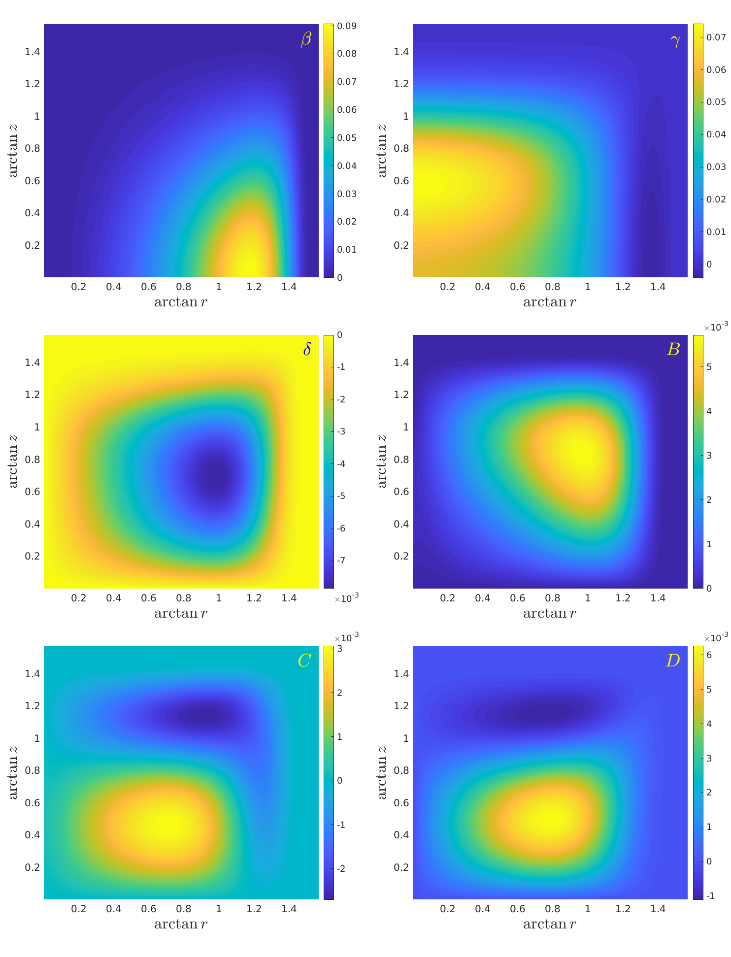
Figure 4: The numerical solution to the equations given in Appendix A, part one.

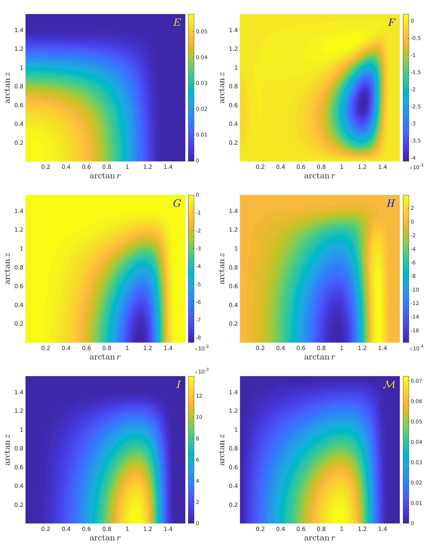
Figure 5: The numerical solution to the equations given in Appendix A, part two.

We perform a change of coordinates

$$\mathsf{x}=\arctan r,\qquad\mathsf{y}=\arctan z,$$ (B.1)

and discretize the latter variables on an equidistant lattice of $512^{2}$ points and use a fourth-order 5-stencil finite difference scheme to calculate the derivatives. We solve the 11 coupled PDEs using a custom built CUDA C code using the relaxation method. To this end, we calculate the solutions for each source term (the latter terms in each of the equations in Appendix B) separately and add the resulting solutions to get a final solution for the fields $\beta$, $\gamma$, $\delta$, $B$, $C$, $D$, $E$, $F$, $G$, $H$, and $I$. Using this solution, we check that the total solution is still satisfying the full system of equation and then we use Eq. (3.21) to calculate $\mathcal{M}$ from which the EDM can be computed using Eq. (5.15). The solution is shown in Figs. 4, 5.

References

- [1] E. M. Purcell and N. F. Ramsey, “On the Possibility of Electric Dipole Moments for Elementary Particles and Nuclei,” Phys. Rev. 78, 807 (1950).
- [2] J. M. Pendlebury et al., “Revised experimental upper limit on the electric dipole moment of the neutron,” Phys. Rev. D 92, no. 9, 092003 (2015) [arXiv:1509.04411 [hep-ex]].
- [3] O. Lebedev, K. A. Olive, M. Pospelov and A. Ritz, “Probing CP violation with the deuteron electric dipole moment,” Phys. Rev. D 70, 016003 (2004) [hep-ph/0402023].
- [4] C.-P. Liu and R. G. E. Timmermans, “P- and T-odd two-nucleon interaction and the deuteron electric dipole moment,” Phys. Rev. C 70, 055501 (2004) [nucl-th/0408060].
- [5] N. Yamanaka and E. Hiyama, “Enhancement of the CP-odd effect in the nuclear electric dipole moment of 6Li,” Phys. Rev. C 91 (2015) no.5, 054005 [arXiv:1503.04446 [nucl-th]].
- [6] N. Yamanaka, “Review of the electric dipole moment of light nuclei,” Int. J. Mod. Phys. E 26 (2017) no.4, 1730002 [arXiv:1609.04759 [nucl-th]].
- [7] J. de Vries, E. Mereghetti, R. G. E. Timmermans and U. van Kolck, “Parity- and Time-Reversal-Violating Form Factors of the Deuteron,” Phys. Rev. Lett. 107 (2011) 091804 [arXiv:1102.4068 [hep-ph]].
- [8] J. de Vries, R. Higa, C.-P. Liu, E. Mereghetti, I. Stetcu, R. G. E. Timmermans and U. van Kolck, “Electric Dipole Moments of Light Nuclei From Chiral Effective Field Theory,” Phys. Rev. C 84 (2011) 065501 [arXiv:1109.3604 [hep-ph]].
- [9] J. Bsaisou, C. Hanhart, S. Liebig, U.-G. Meissner, A. Nogga and A. Wirzba, “The electric dipole moment of the deuteron from the QCD -term,” Eur. Phys. J. A 49 (2013) 31 [arXiv:1209.6306 [hep-ph]].
- [10] J. Bsaisou, J. de Vries, C. Hanhart, S. Liebig, U. G. Meissner, D. Minossi, A. Nogga and A. Wirzba, “Nuclear Electric Dipole Moments in Chiral Effective Field Theory,” JHEP 1503 (2015) 104, Erratum: [JHEP 1505 (2015) 083] [arXiv:1411.5804 [hep-ph]].
- [11] J. Pretz [JEDI Collaboration], “Measurement of Permanent Electric Dipole Moments of Charged Hadrons in Storage Rings,” Hyperfine Interact. 214, no. 1-3, 111 (2013) [arXiv:1301.2937 [hep-ex]].
- [12] E. Witten, “Anti-de Sitter space, thermal phase transition, and confinement in gauge theories,” Adv. Theor. Math. Phys. 2, 505 (1998) [hep-th/9803131].
- [13] T. Sakai and S. Sugimoto, “Low energy hadron physics in holographic QCD,” Prog. Theor. Phys. 113, 843 (2005) [hep-th/0412141].
- [14] T. Sakai and S. Sugimoto, “More on a holographic dual of QCD,” Prog. Theor. Phys. 114, 1083 (2005) [hep-th/0507073].
- [15] L. Bartolini, F. Bigazzi, S. Bolognesi, A. L. Cotrone and A. Manenti, “Theta dependence in Holographic QCD,” JHEP 1702, 029 (2017) [arXiv:1611.00048 [hep-th]].
- [16] L. Bartolini, F. Bigazzi, S. Bolognesi, A. L. Cotrone and A. Manenti, “Neutron electric dipole moment from gauge/string duality,” Phys. Rev. Lett. 118, no. 9, 091601 (2017) [arXiv:1609.09513 [hep-ph]].
- [17] E. Shintani, T. Blum, T. Izubuchi and A. Soni, “Neutron and proton electric dipole moments from domain-wall fermion lattice QCD,” Phys. Rev. D 93, no. 9, 094503 (2016) [arXiv:1512.00566 [hep-lat]].
- [18] F.-K. Guo et al., “The electric dipole moment of the neutron from 2+1 flavor lattice QCD,” Phys. Rev. Lett. 115, no. 6, 062001 (2015) [arXiv:1502.02295 [hep-lat]].
- [19] C. Alexandrou, A. Athenodorou, M. Constantinou, K. Hadjiyiannakou, K. Jansen, G. Koutsou, K. Ottnad and M. Petschlies, “Neutron electric dipole moment using twisted mass fermions,” Phys. Rev. D 93, no. 7, 074503 (2016) [arXiv:1510.05823 [hep-lat]].
- [20] A. Shindler, T. Luu and J. de Vries, “Nucleon electric dipole moment with the gradient flow: The -term contribution,” Phys. Rev. D 92, no. 9, 094518 (2015) [arXiv:1507.02343 [hep-lat]].
- [21] R. J. Crewther, P. Di Vecchia, G. Veneziano and E. Witten, “Chiral Estimate of the Electric Dipole Moment of the Neutron in Quantum Chromodynamics,” Phys. Lett. 88B, 123 (1979), Erratum: [Phys. Lett. 91B, 487 (1980)].
- [22] L. J. Dixon, A. Langnau, Y. Nir and B. Warr, “The Electric dipole moment of the neutron in the Skyrme model,” Phys. Lett. B 253, 459 (1991).
- [23] P. Salomonson, B. S. Skagerstam and A. Stern, “Electric dipole moment of the neutron in the two flavor Skyrme model,” Mod. Phys. Lett. A 6, 3647 (1991).
- [24] J. M. Maldacena, “The Large N limit of superconformal field theories and supergravity,” Int. J. Theor. Phys. 38, 1113 (1999) [Adv. Theor. Math. Phys. 2, 231 (1998)] [hep-th/9711200].
- [25] D. K. Hong, M. Rho, H. U. Yee and P. Yi, “Chiral Dynamics of Baryons from String Theory,” Phys. Rev. D 76, 061901 (2007) [hep-th/0701276 [hep-th]].
- [26] H. Hata, T. Sakai, S. Sugimoto and S. Yamato, “Baryons from instantons in holographic QCD,” Prog. Theor. Phys. 117, 1157 (2007) [hep-th/0701280 [hep-th]].
- [27] K. Hashimoto, T. Sakai and S. Sugimoto, “Holographic Baryons: Static Properties and Form Factors from Gauge/String Duality,” Prog. Theor. Phys. 120, 1093 (2008) [arXiv:0806.3122 [hep-th]].
- [28] S. Bolognesi and P. Sutcliffe, “The Sakai-Sugimoto soliton,” JHEP 1401, 078 (2014) [arXiv:1309.1396 [hep-th]].
- [29] O. Aharony and D. Kutasov, “Holographic Duals of Long Open Strings,” Phys. Rev. D 78, 026005 (2008) [arXiv:0803.3547 [hep-th]].
- [30] K. Hashimoto, T. Hirayama and D. K. Hong, “Quark Mass Dependence of Hadron Spectrum in Holographic QCD,” Phys. Rev. D 81, 045016 (2010) [arXiv:0906.0402 [hep-th]].
- [31] S. Baldino, S. Bolognesi, S. B. Gudnason and D. Koksal, “Solitonic approach to holographic nuclear physics,” Phys. Rev. D 96, no. 3, 034008 (2017) [arXiv:1703.08695 [hep-th]].
- [32] Y. Kim, S. Lee and P. Yi, “Holographic Deuteron and Nucleon-Nucleon Potential,” JHEP 0904, 086 (2009) [arXiv:0902.4048 [hep-th]].