Optimal Algorithms for Geometric Centers and Depth

Abstract

We develop a general randomized technique for solving implicit linear programming problems, where the collection of constraints are defined implicitly by an underlying ground set of elements. In many cases, the structure of the implicitly defined constraints can be used to obtain faster linear program solvers.

We apply this technique to obtain near-optimal algorithms for a variety of fundamental problems in geometry. For a given point set $P$ of size $n$ in $\mathbb{R}^{d}$, we develop algorithms for computing geometric centers of a point set, including the centerpoint and the Tukey median, and several other more involved measures of centrality. For $d=2$, the new algorithms run in $O(n\log n)$ expected time, which is optimal, and for higher constant $d>2$, the expected time bound is within one logarithmic factor of $O(n^{d-1})$, which is also likely near optimal for some of the problems.

1 Introduction

Parametric search

In the 1980s, Nimrod Megiddo came up with an ingenious technique for solving efficiently many geometric optimization problems. This parametric-search technique [AS98, Meg83] works by parallelizing a decider procedure for the problem (i.e., an algorithm that can solve the decision problem associated with the optimization problem), and conceptually running it on the unknown parameter being the optimal value. One then simulates the execution of this parallel algorithm. This reduces to resolving a large batch of parallel comparisons performed by the algorithm (i.e., the critical values of the problem), which is done by performing a binary search over these critical values using a sequential decider algorithm. The details of the resulting algorithm, being a mixed simulation of a parallel algorithm, tends to be convoluted, complicated and counter-intuitive. Nevertheless, this technique provides the optimal or fastest deterministic algorithm for many geometric optimization problems.

Linear programming (LP)

Remarkably, in roughly the same time, Nimrod Megiddo [Meg84] came up with a linear time algorithm for linear programming in constant dimension. His algorithm shares some ideas with his parametric search technique. This algorithm can be dramatically simplified (and in practice sped up) by using randomization [Sei91, Kal92, Cla95, MSW96]. Here is a quick sketch of Seidel’s algorithm [Sei91]—it randomly permutes the constraints, inserts them one by one, and checks whether an inserted constraint violates the current optimal solution. If so, it recurses on the offending constraint (and the prefix of the constraints inserted so far). The probability that the $i$th constraint violates the current solution is $O(1/i)$, which implies that the expected number of recursive calls in the top level is $O(\log n)$. Since the violation check takes constant time, and the recursion depth is bounded, this readily implies a running time that is near linear. A somewhat more careful analysis shows that the expected running time is linear.

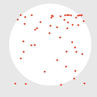
(A)	(B)
(C)	(D)

Figure 1.1: (A) Points. (B) Median lines and the extremal yolk. (C) All lines and the egg. (D) Points with the extremal yolk and the egg.

Randomization for parametric search

It is by now well known [OV04] that randomization can be used as a replacement to parametric search, resulting in simpler (and in many cases faster) algorithms. In particular, Chan [Cha99] identified a surprisingly simple and efficient algorithmic technique that can be used to solve many of these geometric optimization problems (it is similar in spirit to Seidel’s algorithm for LP). Specifically, imagine a maximization problem where one has a fast decider algorithm that can tell us whether a given value is larger or smaller than the optimal value of the given instance. Furthermore, assume that the problem at hand can be (quickly) divided into a small number (e.g., constant) of smaller instances, such that the value of one of these instances is the desired optimal value, and all the other instances have values that are not larger. Chan’s algorithm now randomly orders these subproblems, and solves the problem recursively on each subproblem, but only if the (fast) decider indicates that the current subproblem contains a higher value solution than the one found so far. If there are $t$ subproblems, the algorithm in expectation performs only $O(\log t)$ recursive calls. The result is a significantly simpler randomized algorithm (which uses the decision algorithm only as a black box), which is also faster and has none of the logarithmic-factor slowdowns that parametric-search suffers from.

In this paper, we develop a generalization of the above randomized optimization technique. This generalized technique is interesting in its own right, as it can handle certain linear programming (LP) problems, where the constraints are too numerous to be explicitly stated and are thus specified implicitly. We apply this technique to a variety of problems, discussed next.

1.1 Motivation & problems studied

1.1.1 Tukey depth

Definition 1.1.

Given a set $P$ of $n$ points in $\mathbb{R}^{d}$, the Tukey depth of a point $p\in\mathbb{R}^{d}$ is

$$\min_{h^{+}:\,\text{halfspace containing }p}|P\cap h^{+}|.$$

The task at hand is to compute a Tukey median, that is, a point $p\in\mathbb{R}^{d}$ with maximum Tukey depth. By the centerpoint theorem, there is always a point of Tukey depth $\geq n/(d+1)$ in $\mathbb{R}^{d}$.

Notions of depths for point data sets are important in statistical analysis. The above definition (also called location depth, data depth, and halfspace depth) is among the most well-known and was popularized by John Tukey [Tuk75], who suggested using the corresponding depth contours (boundaries of regions of all points with equal depth) to visualize data. A Tukey median can serve as a point estimator for the data set (a “center”) which is robust against outliers, does not rely on distances, and is invariant under affine transformations [RR98, RR96, Sma90].

Because of the applications to statistics, the issue of designing efficient algorithms to find Tukey medians and their relatives—for example, a point with maximum Liu/simplicial depth, minimum Oja depth, or maximum convex-layers/peeling depth, and a line or flat with maximum regression depth—has attracted a great deal of attention from researchers in computational geometry. See [ACG+02, ALST03, BE02, GSW92, KMR+08, LS00, LS03, LS03a, MRR+03] for the definitions of these concepts and relevant algorithms.

1.1.2 Voting games and the yolk

Suppose there is a collection of $n$ voters in $\mathbb{R}^{d}$, where each coordinate represents a specific ideology. In each coordinate, each voter has a value representing their stance on a given ideology. One can interpret $\mathbb{R}^{d}$ as a policy space, and each point in $\mathbb{R}^{d}$ represents a single policy. In the Euclidean spatial model, a voter $p\in\mathbb{R}^{d}$ always prefers policies which are closer to $p$ under the Euclidean norm. For two policies $x,y\in\mathbb{R}^{d}$ and a set of voters $P\subset\mathbb{R}^{d}$, $x$ beats $y$ if more voters in $P$ prefer policy $x$ compared to $y$. A plurality point is a policy which beats all other policies in $\mathbb{R}^{d}$. For $d=1$, the plurality point is the median voter (when $n$ is odd) [Bla48]. However for $d>1$, a plurality point is not always guaranteed to exist [Rub79]. It is known that one can test whether a plurality point exists (and if so, compute it) in $O(dn\log n)$ time [BGM18]. Note that the plurality point is a point of Tukey depth $\left\lceil{n/2}\right\rceil$—in general this is the largest possible Tukey depth any point can have; while the centerpoint is a point that guarantees a “respectable” minority of size at least $n/(d+1)$.

Since plurality points may not always exist, one generalization of a plurality point is the yolk [McK86]. A hyperplane is a median hyperplane if the number of voters lying in each of the two closed halfspaces (bounded by the hyperplane) is at least $\left\lceil{n/2}\right\rceil$. The yolk is the ball of smallest radius intersecting all such median hyperplanes. Note that when a plurality point exists, the yolk has radius zero (equivalently, all median hyperplanes intersect at a common point).

In terms of real world politics, one can think of the yolk as representing an area of ambiguity where the policy of a political party might be located. Such an ambiguity might be intentional, or the natural consequence of forming a party made out of people with differing views.

We also consider the following restricted problem. A hyperplane is extremal if and only if it passes through $d$ input points, under the assumption that the points are in general position. The extremal yolk is the ball of smallest radius intersecting all extremal median hyperplanes. Importantly, the yolk and the extremal yolk are different problems—the radius of the yolk and extremal yolk can differ [ST92].

1.1.3 The egg of a point set

A problem related to computing the yolk is the following: For a set of $n$ points $P$ in $\mathbb{R}^{d}$, compute the smallest radius ball intersecting all extremal hyperplanes of $P$ (i.e., all hyperplanes passing through $d$ points of $P$). Such a ball is the egg of $P$. See Figure 1.1 for an illustration of the yolk and egg of a point set.

1.1.4 Linear programs with many implicit constraints

Many of the problems discussed above (e.g., computing the Tukey median or egg of a point set) can be written as an LP with $\Theta(n^{d})$ constraints, defined implicitly by the point set $P$. One can apply Seidel’s algorithm [Sei91] (or any other linear time LP solver in constant dimension) to obtain an $O(n^{d})$ expected time algorithm for our problems. However, as each $d$-tuple of points forms a constraint, it is natural to ask if one can obtain a faster algorithm in this setting. Specifically, we are interested in the following problem: Let $I$ be an instance of a $d$-dimensional LP specified via a set of $n$ entities $P$, where each $k$-tuple of $P$ induces a linear constraint in $I$, for some (constant) integer $k$. The problem is to efficiently solve $I$, assuming access to some additional subroutines. (We would also be interested in the more general settings where not all the tuples induce constraints.)

1.2 Previous work

1.2.1 On computing a Tukey median

For dimension $d=1$, a Tukey median corresponds to the standard median, and can be computed in linear time [CLRS01], with the maximum depth being (exactly) $\left\lceil{n/2}\right\rceil$.

For $d>1$, the maximum Tukey depth is between $\left\lceil{n/(d+1)}\right\rceil$ and $\left\lceil{n/2}\right\rceil$. The lower bound follows from the existence of a centerpoint, which follows from Helly’s theorem. A centerpoint has depth at least $\left\lceil{n/(d+1)}\right\rceil$. The first nontrivial algorithmic result in the plane, by Cole et al. [CSY87], presented an algorithm for computing a centerpoint in $O(n\log^{5}n)$ time, using a two-level application of parametric search [Meg83]. Cole’s refined parametric-search technique [Col87] subsequently reduced the time bound to $O(n\log^{3}n)$. Later, an $O(n)$ time algorithm for centerpoints in the plane was discovered by Jadhav and Mukhopadhyay [JM94], using a clever prune-and-search approach. This algorithm does not solve the (more general) Tukey median problem.

In 1991, Matoušek [Mat90] described an algorithm that decides, in $O(n\log^{4}n)$ time, whether the maximum Tukey depth is at least a given value $k$, using also a two-level parametric search as a subroutine. His algorithm constructs a description of the entire region of all points at depth at least $k$. Consequently, a binary search over $k$ yields the maximum Tukey depth and a Tukey median in $O(n\log^{5}n)$ time.

In 2000, Langerman and Steiger [LS00] obtained a faster decision algorithm with an $O(n\log^{3}n)$ running time by using an alternative to parametric search. This algorithm avoids constructing the entire depth region. The additional binary search then leads to an $O(n\log^{4}n)$ time bound for Tukey median. Subsequently, Langerman and Steiger [LS03a] showed that the Tukey median problem itself can be solved in $O(n\log^{3}n)$ time. Some extra logarithmic factors seem inherent in their binary-search-like approach. There is an $\Omega(n\log n)$ lower bound on the time complexity of (i) computing the maximum Tukey depth, (ii) deciding whether the maximum depth is at least $k$, (iii) the depth value of just a single point $q$, or (iv) finding a Tukey median that is extreme along a given direction [ALST03, LS00]. We conjecture that the $\Omega(n\log n)$ lower bound holds for finding an arbitrary Tukey median as well.

Extensions to $d=3$ were also considered. An $O(n^{2}\,\text{polylog}\,n)$ algorithm for computing a 3-dimensional centerpoint was given by Naor and Sharir [NS90]. More recently, Agarwal, Sharir, and Welzl [ASW08] and Oh and Ahn [OA19] gave more near-quadratic algorithms (with extra $n^{o(1)}$ or polylogarithmic factors) for computing the entire region of all points of depth at least $k$ in 3 dimensions.

Note that the problem is difficult because of our insistence on using exact depth values. Approximate versions of the problem can be solved considerably more quickly; for example, see [CEM+96, HJ19, Mat90].

1.2.2 On computing the yolk

Both the yolk and the extremal yolk have been studied in the literature. The first polynomial time exact algorithm for computing the yolk in $\mathbb{R}^{d}$ was by Tovey in $O\bigl{(}n^{(d+1)^{2}}\bigr{)}\Bigr{.}$ time—in the plane, the running time can be improved to $O(n^{4})$ [Tov92]. Following Tovey, recent results have focused on computing the yolk in the plane. In 2018, de Berg et al. [BGM18] gave an $O(n^{4/3}\log^{1+o(1)}n)$ time algorithm for computing the yolk. The running time follows from the best known upper bound on the number of combinatorially distinct median lines, which is $O(n^{4/3})$ [Dey98]. Obtaining a faster exact algorithm remained an open problem. Gudmundsson and Wong [GW19, GW19a] presented a $(1+\varepsilon)$-approximation algorithm with $O(n\log^{7}n\log^{4}\varepsilon^{-1})$ running time. An unpublished result of de Berg et al. [BCG19] achieves a randomized $(1+\varepsilon)$-approximation algorithm for the extremal yolk running in expected time $O(n\varepsilon^{-3}\log^{3}n)$.

1.2.3 On computing the egg

The egg of a point set in $\mathbb{R}^{d}$ can be computed by solving a linear program with $\Theta(n^{d})$ constraints. The egg is a natural extension to computing the yolk, and thus obtaining faster exact algorithms is of interest. The authors are not aware of any previous work on this specific problem. Bhattacharya et al. [BJMR94] gave an algorithm which computes the smallest radius ball intersecting a set of $m$ hyperplanes in $O(m)$ time, when $d=O(1)$, by formulating the problem as an LP (see also Lemma 6.4). However we emphasize that in our problem the set of hyperplanes is implicitly defined by the point set $P$, and is of size $\Theta(n^{d})$ in $\mathbb{R}^{d}$.

$d=2$	$(1+\varepsilon)$-approx	Exact	Our results (Exact)
Extremal yolk	$O(n\varepsilon^{-3}\log^{3}n)$ [BCG19]	$O(n^{4/3}\log^{1+\epsilon}n)$ [BGM18]	$O(n\log n)$ Theorem 6.9
Yolk	$O(n\log^{7}n\log^{4}\varepsilon^{-1})$ [GW19a]	$O(n^{4/3}\log^{1+\epsilon}n)$ Variant of [BGM18]	$O(n\log n)$ Theorem 7.5
$d\geq 3$
Extremal yolk	?	$O(n^{d})$ Known techniques	$O(n^{d-1}\log n)$ Theorem 6.9
Yolk	?	$O(n^{d})$ Known techniques	$O(n^{d-1})$ Theorem 7.5

Table 1.1: Some previous work on the yolk and our results. Existing algorithms are deterministic, while the running time of our algorithms holds in expectation.

1.3 Our results

In this paper we develop a generalized technique for solving LPs with many implicitly defined constraints. The new technique has specific requirements to be met so it can be used, and these are spelled out in Section 4.1.1. Informally, these requirements are:

1. The problem can be solved in constant time for constant size instances.

2. Given a candidate solution for an instance of size $n$, one can verify that it is optimal, in $\mathcal{D}\left({n}\right)$ time.

3. One can break the given instance, in $\mathcal{D}\left({n}\right)$ time, into a constant number of smaller (by a constant factor) instances, such that the union of the implicit constraints they induce is the set of original constraints.

4. The function $\mathcal{D}\left({n}\right)$ grows fast enough.

Under these requirements, the implicit LP problem can be solved in $O\bigl{(}\mathcal{D}\left({n}\right)\bigr{)}$ time.

In Section 4 we state the technique and prove the key result (Theorem 4.5). The technique builds on the work of Chan [Cha99] and leads to efficient algorithms for the following problems. Throughout, let $P\subset\mathbb{R}^{d}$ be a set of $n$ points in general position:

1. In Section 5 we show that the point of maximum Tukey depth can be computed in $O(n^{d-1}+n\log n)$ expected time. As the problem of detecting affine degeneracies (the existence of $d$ points on a common hyperplane) among $n$ points in $\mathbb{R}^{d-1}$ is believed to require $\Omega(n^{d-1})$ time [Eri99] and can be reduced to computing the maximum Tukey depth in $\mathbb{R}^{d}$, our result is likely to be optimal for $d\geq 3$ as well. Note that as a byproduct, we get an improved $O(n^{2})$ time randomized algorithm for centerpoints in $\mathbb{R}^{3}$.

2. In Section 5.1.4 we show how to compute in the plane the convex polygon forming the points of Tukey depth at least $k$. The new algorithm has running time $O(n\log^{2}n)$, and improves over the work of Matoušek [Mat90], that worked in $O(n\log^{4}n)$ time.

3. The yolk of $P$ can be computed exactly in $O(n^{d-1}+n\log n)$ expected time. The extremal yolk can be computed in $O(n^{d-1}\log n)$ time. Hence in the plane, the yolk can be computed in $O(n\log n)$ expected time. This improves all existing algorithms (both exact and approximate) [Tov92, BGM18, GW19a, GW19, BCG19] for computing the yolk in the plane, and our algorithm easily generalizes to higher dimensions. See Table 1.1 for a summary of our results and previous work.

4. By a straightforward modification of the above algorithm, in Lemma 6.10, we prove that the egg of $P$ can be computed in $O(n^{d-1}\log n)$ expected time.

5. Let $H_{k}(P)$ be the collection of all open halfspaces which contain more than $n-k$ points of $P$. Consider the convex polygon $\mathcal{T}_{k}=\bigcap_{h\in H_{k}(P)}h$. Observe that $\mathcal{T}_{1}$ is the convex hull of $P$, with $\mathcal{T}_{1}\supseteq\mathcal{T}_{2}\supseteq\cdots$. The centerpoint theorem implies that $\mathcal{T}_{n/(d+1)}$ is non-empty (and contains the centerpoint). The Tukey depth of a point $q$ is the minimal $k$ such that $q\in\mathcal{T}_{k}\setminus\mathcal{T}_{k+1}$.

   When $\mathcal{T}_{k}$ is non-empty, the center ball of $P$ is the ball of largest radius contained inside $\mathcal{T}_{k}$. For $\mathcal{T}_{k}$ empty, we define the Tukey ball of $P$ as the smallest radius ball intersecting all halfspaces of $H_{k}(P)$.

   In Section 8 we show that the Tukey ball and center ball can both be computed in $\scalerel*{\widetilde{O}}{j^{2}}\bigl{(}k^{d-1}\big{[}1+(n/k)^{\left\lfloor{d/2}\right\rfloor}\big{]}\bigr{)}$ expected time (see Lemma 8.5 and Lemma 8.8, respectively), where $\scalerel*{\widetilde{O}}{j^{2}}$ hides polylog terms. In particular, when $k$ is a (small) constant, a point of Tukey depth $k$ can be computed in time $\scalerel*{\widetilde{O}}{j^{2}}(n^{\left\lfloor{d/2}\right\rfloor})$. As mentioned above, for $k\leq n/(d+1)$, the centerpoint has Tukey depth $\geq k$. As such, the issue here is computing such a point (and not deciding its existence). This improves on the algorithm for computing a point of Tukey depth at least $k$, when $k\ll n$.

6. In Section 9, we present the last application: Given a set $L$ of $n$ lines in the plane, the crossing distance between two points $p,q\in\mathbb{R}^{2}$ is the number of lines of $L$ intersecting the segment $pq$. Given a point $q\in\mathbb{R}^{2}$ not lying on any lines of $L$, the disk of smallest radius containing all vertices of $\mathcal{A}\left({L}\right)$ within crossing distance at most $k$ from $q$ can be computed in $O(n\log n)$ expected time. See Lemma 9.1.

Paper organization

We provide some needed preliminaries in Section 2. We study some variants of LP-type problems in Section 3 – specifically, ranking and batched LP-type problems. The main technique is presented in Section 4. We present an algorithm for the Tukey depth problem in Section 5. The algorithm for the extremal yolk is presented in Section 6. The algorithm for the continuous yolk is presented in Section 7. The algorithms for Tukey ball and center ball are presented in Section 8. In Section 9, we present the algorithm for computing the smallest disk within certain crossing distance. We conclude in Section 10 with a few final remarks.

2 Preliminaries

Notation

Throughout, the $O$ notation hides factors which depend (usually exponentially) on the dimension $d$. Additionally, the $\scalerel*{\widetilde{O}}{j^{2}}$ notation hides factors of the form $\log^{c}n$, where $c$ is a constant that may depend on $d$.

2.1 Duality

Definition 2.1 (Duality).

The dual hyperplane of a point $p=(p_{1},\ldots,p_{d})\in\mathbb{R}^{d}$ is the hyperplane $p^{\star}$ defined by the equation $x_{d}=-p_{d}+\sum_{i=1}^{d-1}x_{i}p_{i}$. The dual point of a hyperplane $h$ defined by $x_{d}=a_{d}+\sum_{i=1}^{d-1}a_{i}x_{i}$ is the point

$$h^{\star}=(a_{1},a_{2},\ldots,a_{d-1},-a_{d}).$$

Fact 2.2.

Let $p$ be a point and let $h$ be a hyperplane. Then $p$ lies above $h$ $\iff$ the hyperplane $p^{\star}$ lies below the point $h^{\star}$.

Given a set of objects $T$ (e.g., points in $\mathbb{R}^{d}$), let $T^{\star}=\left\{x^{\star}\;\middle|\;x\in T\right\}$ denote the dual set of objects.

2.2 $k$-Levels

Definition 2.3 (Levels).

For a collection of hyperplanes $H$ in $\mathbb{R}^{d}$, the level of a point $p\in\mathbb{R}^{d}$, denoted by $\mathrm{level}\left({p}\right)$, is the number of hyperplanes of $H$ lying on or below $p$. The bottom $k$-level of $H$ is the (closure of the) union of points in $\mathbb{R}^{d}$ which have level equal to $k$, and let $B_{k}(H)$ denote the set of all such points. The (bottom) $(\leq k)$-level of $H$ is the union of points in $\mathbb{R}^{d}$ which have level at most $k$. Let $B_{<k}(H)=\bigcup_{i=0}^{k-1}B_{i}(H)$.

The top $k$-level is defined analogously (i.e., all points that have $k$ hyperplanes above them). We denote the top $k$-level by $T_{k}(H)$. Let $T_{<k}(H)=\bigcup_{i=0}^{k-1}T_{i}(H)$.

By Fact 2.2, if $h$ is a hyperplane which contains $k$ points of $P$ lying on or above it, then the dual point $h^{\star}$ is a member of the $k$-level of $P^{\star}$.

2.3 Zones of surfaces

For a set of hyperplanes $H$, denote the arrangement of $H$ by $\mathcal{A}\left({H}\right)$ (see, e.g., [BCKO08]).

Definition 2.4 (Zone of a surface).

For a collection of hyperplanes $H$ in $\mathbb{R}^{d}$, the complexity of a cell $\psi$ in the arrangement $\mathcal{A}\left({H}\right)$ is the number of faces (of all dimensions) which are contained in the closure of $\psi$. For a $(d-1)$-dimensional surface $\gamma$, the zone $\mathcal{Z}\left({\gamma,H}\right)$ of $\gamma$ is the subset of cells of $\mathcal{A}\left({H}\right)$ which intersect $\gamma$. The complexity of a zone is the sum of the complexities of the cells in $\mathcal{Z}\left({\gamma,H}\right)$.

The complexity of a zone of a hyperplane is known to be $\Theta(n^{d-1})$ [ESS93]. For general algebraic surfaces it is larger by a logarithmic factor. Furthermore, the cells in the zone of a surface can be computed efficiently using lazy randomized incremental construction [BDS95].

Lemma 2.5 ([APS93, BDS95]).

Let $H$ be a set of $n$ hyperplanes in $\mathbb{R}^{d}$ and let $\gamma$ be a $(d-1)$-dimensional algebraic surface of degree $\delta$. The complexity of the zone $\mathcal{Z}\left({\gamma,H}\right)$ is $O(n^{d-1}\log n)$, where the hidden constants depend on $d$ and $\delta$. The collection of cells in $\mathcal{Z}\left({\gamma,H}\right)$ can be computed in $O(n^{d-1}\log n)$ expected time.

2.4 Cuttings

Definition 2.6 (Cuttings).

Given $n$ hyperplanes in $\mathbb{R}^{d}$, a $(1/c)$-cutting is a collection of interior disjoint simplices covering $\mathbb{R}^{d}$, such that each simplex intersects at most $n/c$ hyperplanes.

Lemma 2.7 ([Cha93]).

Given a collection of $n$ hyperplanes in $\mathbb{R}^{d}$, a $(1/c)$-cutting of size $O(c^{d})$ can be constructed in $O(nc^{d-1})$ time.

2.5 LP-type problems

An LP-type problem, introduced by Sharir and Welzl [SW92], is a generalization of a linear program. Let ${H}$ be a set of constrains and $f$ be an objective function. For any $\mathcal{B}\subseteq{H}$, let $f\left({\mathcal{B}}\right)$ denote the value of the optimal solution for the constraints of $\mathcal{B}$. The goal is to compute $f\left({{H}}\right)$. If the problem is infeasible, let $f\left({{H}}\right)=\infty$. Similarly, define $f\left({{H}}\right)=-\infty$ if the problem is unbounded.

Definition 2.8.

Let ${H}$ be a set of constraints, and let $f:2^{H}\to\mathbb{R}\cup\{\infty,-\infty\}$ be an objective function. The tuple $({H},f)$ forms an LP-type problem if the following properties hold:

1. Monotonicity. For any ${B}\subseteq{C}\subseteq{H}$, we have $f\left({{B}}\right)\leq f\left({{C}}\right)$.

2. Locality. For any ${B}\subseteq{C}\subseteq{H}$ with $f\left({{C}}\right)=f\left({{B}}\right)>-\infty$, and for all $s\in{H}$, $f\left({{C}}\right)<f\left({{C}+s}\right)\iff f\left({{B}}\right)<f\left({{B}+s}\right)$, where ${B}+s={B}\cup\left\{{s}\right\}$.

A basis of a set ${H}^{\prime}\subseteq{H}$ is an inclusion-wise minimal subset $\mathcalb{b}\subseteq{H}^{\prime}$ with $f\left({\mathcalb{b}}\right)=f\left({{H}^{\prime}}\right)$. The combinatorial dimension $\delta$ is the maximum size of any feasible basis of any subset ${H}^{\prime}$ of ${H}$. Throughout, we consider $\delta$ to be a constant. For a basis $\mathcalb{b}\subseteq{H}$, a constraint $h\in{H}$ violates the current solution induced by $\mathcalb{b}$ if $f\left({\mathcalb{b}+h}\right)>f\left({\mathcalb{b}}\right)$. LP-type problems with $n$ constraints can be solved in randomized time $O(n)$, hiding constants depending (exponentially) on $\delta$ [Cla95], where the bound on the running time holds with high probability.

Remark 2.9.

The aforementioned algorithms for solving LP-type problems require certain primitives to be provided, such as testing for a basis violation, and computing the basis for a small set of constraints. In the following, we assume that such primitives are provided when considering any LP-type problem.

3 Variants of LP-type problems

3.1 Ranking LP-type problem

Let ${H}$ be a set of constraints, and assume that each constraint $h$ has an associated rank $\mathrm{r}\left({h}\right)\in\mathbb{R}^{+}$ (importantly for our purposes, the ranks are not necessarily distinct). Assume that $({H},f)$ forms an instance of LP-type (minimization) problem. This instance might not be feasible (i.e., $f\left({{H}}\right)=+\infty$), so consider the parameterized instance. Here, for a number $\alpha\in\mathbb{R}$, we consider the LP-type problem instance $\mathcal{I}(\alpha)$ formed by the set of constraints

$${H}_{\geq\alpha}=\left\{h\in{H}\;\middle|\;\mathrm{r}\left({h}\right)\geq\alpha\right\}.$$

Let $\zeta\left({{H}}\right)$ be the minimum positive real value of $\alpha$ such that ${H}_{\geq\alpha}$ is feasible. For a set of constraints ${B}\subseteq{H}$, consider the target function $g({B})=(\alpha,\beta)$, where $\alpha=\zeta\left({{B}}\right)$ and $\beta=f\left({{B}_{\geq\alpha}}\right)$. Let $\prec$ be the lexicographical ordering of $\mathbb{R}^{2}$ (i.e., $(x,y)\prec(x^{\prime},y^{\prime})$ $\iff$ $x<x^{\prime}$ or [$x=x^{\prime}$ and $y<y^{\prime}$]). The new optimization problem $({H},g)$, is to compute $g({H})$. Thus computing the minimum $\alpha$, such that ${H}_{\geq\alpha}$ is feasible, and the associated original LP value for this subset. We refer to $({H},g)$ as the ranking problem associated with $({H},f)$.

Lemma 3.1.

Given an LP-type problem $({H},f)$ of combinatorial dimension $d$, with associated ranks on the constraints of ${H}$, the ranking problem $({H},g)$ is an LP-type problem of combinatorial dimension $d+1$.

Proof:

The proof is straightforward, and we include it only for the sake of completeness.

The basis of $g({H})$ is a minimal set $\mathcalb{b}\subseteq{H}$, such that $g(\mathcalb{b})=g({H})$. A constraint ${x}\in{H}$ violates $\mathcalb{b}$, if $\mathrm{r}\left({{x}}\right)\geq\mathrm{r}\left({\mathcalb{b}}\right)$ and $f(\mathcalb{b}+{x})>f(\mathcalb{b})$, where $\mathrm{r}\left({\mathcalb{b}}\right)=\min_{h\in\mathcalb{b}}\mathrm{r}\left({h}\right)$. As such, a basis of the ranking problem, is a basis of the original problem with potentially one additional constraint that realizes/records the minimum realizable rank subset.

We now verify the required LP properties from Definition 2.8:

1. Monotonicity: For any ${B}\subseteq{C}\subseteq{H}$, let $\alpha$ be the minimum value such that ${C}_{\geq\alpha}$ is feasible for $f$. Clearly, ${B}_{\geq\alpha}\subseteq{C}_{\geq\alpha}$, which implies that ${B}_{\geq\alpha}$ is feasible for $f$. That is, we have $g({B})\preceq g({C})$.

2. Locality: Consider any ${B}\subseteq{C}\subseteq{H}$ with $g({C})=g({B})\succ(0,-\infty)$.

   Consider any $s\in{H}$, such that $(\alpha,\beta)=g({C})\prec g({C}+s)=(\alpha^{\prime},\beta^{\prime})$. If $\alpha=\alpha^{\prime}$ then $\beta=f({B}_{\geq\alpha})<f({B}_{\geq\alpha}+s)=\beta^{\prime}$. The locality of $f$ implies that $f({C}_{\geq\alpha})<f({C}_{\geq\alpha}+s)$. This implies that $g({B})\prec g({B}+s)$, which implies the locality property.

   Otherwise, $\alpha^{\prime}>\alpha$. This implies that ${C}_{\geq\alpha}+s$ is not feasible, which implies $f({C}_{\geq\alpha})<f({C}_{\geq\alpha}+s)$. By the locality of $f$, we have that $f({B}_{\geq\alpha}+s)>f({B}_{\geq\alpha})$. But that readily implies that $g({B}+s)\succ g({B})=(\alpha,\beta)$.

   As for the other direction, if $g({B})\prec g({B}+s)$ then by monotonicity, we have that $g({C})\prec g({C}+s)$, which implies locality.

 

3.2 Batched LP

Intuitively, one can group constraints of an LP-type problem so that each group form its own “constraint”, and the modified problem remains an LP-type problem. This is captured by the following definition.

Definition 3.2 (Batched LP-type problems).

Let $({H},f)$ be an LP-type problem. A batched LP-type problem is defined by the constraint set $2^{H}$ and the objective function $\mathsf{F}:2^{2^{H}}\to\mathbb{R}\cup\{\infty,-\infty\}$. For non-empty ${B}_{1},\ldots,{B}_{m}\subseteq{H}$, define $\mathsf{F}(\{{B}_{1},\ldots,{B}_{m}\}):=f({B}_{1}\cup\ldots\cup{B}_{m})$.

Lemma 3.3.

Let $({H},f)$ be an LP-type problem of combinatorial dimension $\delta$, and let $\mathcal{H}=2^{H}$. Then $(\mathcal{H},\mathsf{F})$ is an LP-type problem with combinatorial dimension $\delta$.

Proof:

The proof of this lemma is straightforward – we provide a proof for the sake of completeness, but the reader is encouraged to skip it. For any sets $\mathcal{B}\subseteq\mathcal{C}\subseteq\mathcal{H}$, we have that

$$\mathsf{F}(\mathcal{B})=f(\cup\mathcal{B})\leq f(\cup\mathcal{C})\leq\mathsf{F}(\mathcal{C}),$$

by the monotonicity of $f$, see Definition 2.8, where $\cup\mathcal{B}=\cup_{X\in\mathcal{B}}X$. This readily implies the monotonicity of $\mathsf{F}$.

For any $\mathcal{B}\subseteq\mathcal{C}\subseteq 2^{H}$ with $\mathsf{F}(\mathcal{C})=\mathsf{F}(\mathcal{B})>-\infty$, and for all ${S}\in\mathcal{H}$, we have that

$$\mathsf{F}\left({\mathcal{C}}\right)<\mathsf{F}\left({\mathcal{C}+{S}}\right)\iff f\left({\cup\mathcal{C}}\right)<f\left({\cup\mathcal{C}\cup{S}}\right)\iff f\left({\cup\mathcal{B}}\right)<f\left({\cup\mathcal{B}\cup{S}}\right)\iff\mathsf{F}\left({\mathcal{B}}\right)<\mathsf{F}\left({\mathcal{B}+{S}}\right),$$

by the locality of $f$. This implies the locality of $\mathsf{F}$.

As for the combinatorial dimension, consider any family of sets

$$\mathcal{B}=\{{B}_{1},\ldots,{B}_{m}\}\subseteq{H},$$

and let ${X}=\{{x}_{1},\ldots,{x}_{t}\}$ be the basis of $f\left({\cup_{i}{B}_{i}}\right)$. By assumption, $t\leq\delta$. Assume, for simplicity of exposition, that ${x}_{i}\in{B}_{i}$, for all $i$. We have that $\mathcal{Z}=\{{B}_{1},\ldots,{B}_{t}\}$ is a basis for $\mathcal{B}$, for $\mathsf{F}$, as

$$\mathsf{F}\left({\mathcal{B}}\right)=f\left({\cup_{i}{B}_{i}}\right)=f\left({{X}}\right)\leq\mathsf{F}\left({\mathcal{Z}}\right)\leq\mathsf{F}\left({\mathcal{B}}\right)\quad\implies\quad\mathsf{F}\left({\mathcal{Z}}\right)=\mathsf{F}\left({\mathcal{B}}\right).$$

That readily implies that the combinatorial dimension of $(\mathcal{H},\mathsf{F})$ is $\delta$.  

3.3 Solving LP-Type problem for bundles using Seidel’s algorithm

Let $\mathcal{I}=({H},f)$ be an instance of an LP-type problem with combinatorial dimension $\delta$.

Definition 3.4.

Given a set ${H}$ of constraints, a subset of $\Upsilon\subseteq{H}$ is a bundle. A collection $\Upsilon_{1},\ldots,\Upsilon_{n}$ of bundles is a cover of ${H}$ if $\bigcup_{i}\Upsilon_{i}={H}$.

For a given cover $\Upsilon_{1},\ldots,\Upsilon_{n}$, and a basis $\mathcalb{b}$, assume that one can compute the basis of $\mathcalb{b}\cup\Upsilon_{i}$ in $\mathcal{D}$ time, for any $i$, by calling a procedure compBasis. Furthermore, assume that one can also check if any of the constraints of $\Upsilon_{i}$ violates $\mathcalb{b}$, in $\mathcal{D}$ time, by calling a procedure violate. It is natural to ask if one can solve $\mathcal{I}$ quickly. This question makes sense if $\mathcal{D}$ is sublinear in the number of constraints in a bundle.

We are going to use a variant of Seidel’s algorithm for solving LP-type problems, which also works for violator spaces [Sei91, Har11, Har16] (other algorithms for solving LP-type problems can be used here). For the sake of completeness, we next sketch this algorithm. See also Figure 3.1.

solveLPType$\left({\mathcalb{b}_{0},\Upsilon_{1},\ldots,\Upsilon_{m}}\right)$ // $\mathcalb{b}_{0}$: initial basis $\left\langle{\Upsilon_{1}^{\prime},\ldots,\Upsilon_{n}^{\prime}}\right\rangle$: random permutation of $\Upsilon_{1},\ldots,\Upsilon_{m}$. for $i=1$ to $m$ do if violate($\Upsilon_{i}^{\prime}$, $\mathcalb{b}_{i-1}$) then $\mathcalb{t}_{i}\leftarrow{{\color[rgb]{0.59,0,0.66}\texttt{\bf{compBasis}}}}\left({\mathcalb{b}_{i-1},\Upsilon_{i}^{\prime}}\right)$ $\mathcalb{b}_{i}\leftarrow{{{\color[rgb]{0.59,0,0.66}\texttt{\bf{solveLPType}}}}}\left({\mathcalb{t}_{i}\cup\mathcalb{b}_{0},\Upsilon_{1}^{\prime},\ldots,\Upsilon_{i}^{\prime}}\right)$ else $\mathcalb{b}_{i}\leftarrow\mathcalb{b}_{i-1}$ return $\mathcalb{b}_{n}$

Figure 3.1: The algorithm for solving LP-type problems.

The input is an initial basis $\mathcalb{b}_{0}$ (made out of at most $\delta$ constraints), and $n$ bundles of constraints $\Upsilon_{1},\ldots,\Upsilon_{n}$. The algorithm picks uniformly at random a permutation $\pi$ of $\left\llbracket n\right\rrbracket=\{1,\ldots,n\}$. In the $i$th iteration, the algorithm adds $\Upsilon_{i}^{\prime}=\Upsilon_{\pi(i)}$ to the current set of constraints, maintaining the optimal solution to ${X}_{i}=\{\Upsilon_{1}^{\prime},\ldots,\Upsilon_{i}^{\prime}\}\cup\mathcalb{b}_{0}$. To this end, the algorithm maintains a basis $\mathcalb{b}_{i}\subseteq{X}_{i}$ of the solution for the constraints of ${X}_{i}$. Initially, the algorithm sets $\mathcalb{b}_{0}=\mathcalb{b}$.

In the beginning of the $i$th iteration, the algorithm uses the violation test (i.e., violate) to decide if any of the constraints of $\Upsilon_{i}^{\prime}$ violates $\mathcalb{b}_{i-1}$. If there is no violation, the algorithm sets $\mathcalb{b}_{i}$ to $\mathcalb{b}_{i-1}$, and continues to the next iteration. Otherwise, the algorithm computes the basis $\mathcalb{t}_{i}$ of $\mathcalb{b}_{i-1}\cup\Upsilon_{i}^{\prime}$ by calling compBasis. The algorithm then computes $\mathcalb{b}_{i}$ by calling itself recursively with the initial “basis” $\mathcalb{t}_{i}\cup\mathcalb{b}_{0}$ and the bundles $\Upsilon_{1}^{\prime},\ldots,\Upsilon_{i}^{\prime}$ (this second call is on LP-type instance with smaller combinatorial dimension). At the end, the algorithm returns $\mathcalb{b}_{m}$ as the basis of the solution.

The correctness of this algorithm is immediate by interpreting this problem as an instance of batched LP. See Lemma 3.3. In particular, in this variant of the algorithm, the depth of the recursion is at most $\delta$ [Har16], and as such the initial “basis” set is of size at most $\delta^{2}$ (i.e., constant). We need the following well known result.

Lemma 3.5 ([SW92, Har11, Har16]).

The input is an instance $\mathcal{I}=({H},f)$ of an LP-type problem with constant combinatorial dimension $\delta$. In addition, the input also includes a cover ${H}$ by $n$ bundles $\Upsilon_{1},\ldots,\Upsilon_{n}$, and procedures violate and compBasis as described above, where each call takes $\mathcal{D}$ time. For this input, the above algorithm computes the optimal solution to $\mathcal{I}$ in $O(n\mathcal{D})$ time, and $O\left({(\delta\log m)^{\delta}}\right)$ calls to compBasis.

Remark 3.6.

It is possible to further reduce the number of calls to compBasis to $O(\delta^{O(\delta)}\log m)$ by using Clarkson’s randomized LP algorithm [Cla95] instead of Seidel’s, though such an improvement will not be needed in our applications.

4 An optimization technique for implicit LP-type problems

The main challenge in implementing the algorithm of Section 3.3 for bundles is that we need to provide the procedures violate and compBasis. A natural approach, if we have a way to break a bundle into subbundles, is to use recursion. For this scheme to make sense, the number of constraints defined by a bundle has to be defined implicitly, and be superlinear in the number of entities defining a bundle.

4.1 Settings and basic idea

4.1.1 Instance of implicit LP

Let $({H},f)$ be an LP-type problem of constant combinatorial dimension $\delta$. Let $\psi$ be an integer constant and $\eta>1$ be another constant. For an input space $\Pi$, suppose that there is a function $g:\Pi\to 2^{H}$ which maps inputs to sets of constraints. Furthermore, assume that for any input $P\in\Pi$ of size $n$, we have the following properties:

1. When $n=O(1)$, a basis for $g(P)$ can be computed in constant time.

2. We are given a violation test that, for a basis $\mathcalb{b}$, decides if $\mathcalb{b}$ satisfies $g(P)$ in $\mathcal{D}\left({n}\right)$ time. (Let violate be the name of this procedure.)

3. In $\mathcal{D}\left({n}\right)$ time, one can construct sets $P_{1},\ldots,P_{\psi}\in\Pi$, each of size at most $n/\eta$, such that $g(P)=\bigcup_{i=1}^{\psi}g(P_{i})$.

4. The function $\mathcal{D}\left({n}\right)/n^{\varepsilon}$ is monotonically increasing for some constant $\varepsilon>0$.

The above is an instance of the implicit LP problem.

Remark 4.1.

Note that the above condition on $\mathcal{D}\left({n}\right)$ in particular implies that for any $1\leq k\leq n$, we have $\mathcal{D}\left({n/k}\right)/(n/k)^{\varepsilon}\leq\mathcal{D}\left({n}\right)/n^{\varepsilon}$, i.e., $\mathcal{D}\left({n/k}\right)\leq\mathcal{D}\left({n}\right)/k^{\varepsilon}$.

4.1.2 An assumption

An annoying technicality is that to bound the running time of the resulting algorithm, we need a strong assumption on the parameters used in the above instance. We tackle issue next, but the casual reader can safely skip to Section 4.1.3.

Specifically, for fixed constants $\varepsilon\in(0,1)$, and $c>1$, the required property is that

$$\frac{c\log^{\delta}\psi}{\eta^{\varepsilon}}<1,$$ (4.1)

where $\psi$ is the number of sets in the partition, and $n/\eta$ is the bound on the size on each set of the partition, see (P3). If the given instance does not have this property, then one can modify the instance, to get a new instance that has this property, as testified by the following.

Lemma 4.2.

Consider a fixed constant $\varepsilon\in(0,1)$, and some fixed constant $c>1$. Given an instance of implicit LP, one can create a new instance such that Eq. (4.1) holds. The asymptotic running time of the new partition procedure is the same.

Proof:

The idea is to apply the decomposition recursively for, say, $i$ levels. We get sets $P_{1},\ldots,P_{m}\subseteq P$, with $m\leq\psi^{i}$, where each set is of size at most $n/\eta^{i}$. This yields a finer decomposition into a larger number of smaller sets, and we can use this decomposition in the above settings. Then

$$c\frac{\log^{\delta}\psi^{i}}{\eta^{\varepsilon i}}=c\frac{i^{\delta}\log^{\delta}\psi}{\eta^{\varepsilon i}}<1,$$

by choosing $i$ to be a sufficiently large constant (depending only on $\psi,\eta,\delta,\varepsilon,c$), since $\eta>1$. Thus, using this decomposition with $\psi^{i}$ sets, and shrinking factor $\eta^{i}$, implies a new instance of the problem that satisfies the claim.  

4.1.3 Example: Egg in the plane

Consider the egg problem in the plane, as defined in Section 1.1.3. The input space $\Pi$ is a set of $n$ points $P$ in the plane. For a pair of points $p,s\in P$, consider the line $\ell$ with equation $\alpha x+\beta y+\gamma=0$ that passes through these two points, where $\alpha^{2}+\beta^{2}=1$. Consider a point $c=(x,y,r)$ in three dimensions. The point $c$ encodes a disk of radius $r$ centered at $(x,y)$. This disk intersects $\ell$ if and only if

$$-r\leq\alpha x+\beta y+\gamma\leq r.$$

This condition corresponds to two linear inequalities, and let $g\bigl{(}\{p,s\})$ denote the set of these two inequalities. For a set $Q\subseteq P$, the associated set of linear constraints is

$$g\bigl{(}Q)=\bigcup_{p,s\in Q,p\neq s}g\bigl{(}\{p,s\}).$$

Thus, to compute the smallest disk intersecting all the lines induced by $P$, we need to solve the three-dimensional LP defined by the constraints of $g\bigl{(}P)$—computing the feasible point with minimum $z$ coordinate. This LP can be solved in quadratic time in a straightforward fashion—here we are interested in solving this problem more quickly.

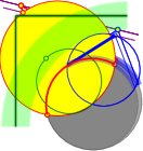
Figure 4.1: Finding an induced line avoiding the disk is equivalent to computing two arcs that intersect but do not contain each other in the associated circular arc graph.

We next verify that the above settings apply. First, the problem can be solved in constant time for a constant size point set. Next, given a basis (i.e., a disk $\mathsf{o}$ in this case), and a set $Q$ of points, one can check (in near linear time) whether two points of $Q$ induce a line that avoids the disk $\mathsf{o}$. An algorithm for this problem is described, in somewhat more abstract settings, in Section 6.2. In this specific case, one can define a circular arc graph on the boundary of $\mathsf{o}$ (see Figure 4.1), where each point $p$ outside $\mathsf{o}$ induces an arc of all the points on the disk boundary that see $p$. On this circular arc graph it is enough to decide if there are two arcs that intersect but do not contain each other, and this can be done, in $O(n\log n)$ time, using “sweeping”. As such, in this case, we have property (P2) with $\mathcal{D}\left({n}\right)=O(n\log n)$.

The divide property, i.e., (P3), is surprisingly straightforward in this case. Partition the point set $P$ into $b$ helper sets $Q_{1},\ldots,Q_{b}$ with $\left|{Q_{i}}\right|\geq\left\lfloor{n/b}\right\rfloor$, for $i\in\left\llbracket b\right\rrbracket=\{1,\ldots,b\}$. For any pair $\{i,j\}\in\binom{\left\llbracket b\right\rrbracket}{2}$ define the point set $P_{i,j}=Q_{i}\cup Q_{j}$. Thus, the constructed sets are the members of $\left\{\smash{P_{i,j}}\;\middle|\;\{i,j\}\in\smash{\binom{\left\llbracket b\right\rrbracket}{2}}\bigr{.}\right\}$. As such, $\psi=\binom{b}{2}$ and $\eta=b/2$. Clearly, for any pair of points $\{p,s\}\in\binom{P}{2}$, there are indices $i,j$, such that $p,s\in P_{i,j}$. This implies that $g(P)=g\bigl{(}\bigcup_{i,j}P_{i,j}\bigr{)}$.

The combinatorial dimension of the associated LP is $3$. We can specifically choose $b=3$, but if we want to satisfy Eq. (4.1) directly without invoking Lemma 4.2, we can pick the smallest $b$ such that $c\log^{3}\binom{b}{2}/(b/2)^{\varepsilon}<1$.

4.2 The algorithm for solving implicit LP

4.2.1 The algorithm in detail

The basic idea is to modify the algorithm of Section 3.3 so that compBasis is implemented recursively, via refinement of the current bundle. So, the input is a set of $n$ elements $P\subseteq\Pi$, and the task is to solve the LP-type problem defined by the set of constraints $g(P)$. For any set $Q\subseteq P$, let $\mathcalb{b}(Q)$ denote the basis of size at most $\delta$ for the constraint set $g(Q)$. By requirement (P2), given a basis $\mathcalb{b}$, we can decide if $f\bigl{(}\mathcalb{b}\cup g(Q)\bigr{)}>f(\mathcalb{b})$ by calling violate.

solveBatchLPT$\left({\mathcalb{b}_{0},R_{1},\ldots,R_{m}}\right)\Bigr{.}$   // $\mathcalb{b}_{0}$: initial basis $\left\langle{R_{1}^{\prime},\ldots,R_{n}^{\prime}}\right\rangle$: random permutation of $R_{1},\ldots,R_{m}$. for $i=1$ to $m$ do if violate($R_{i}^{\prime}$, $\mathcalb{b}_{i-1}$) then $\mathcalb{t}_{i}\leftarrow{{\color[rgb]{0.59,0,0.66}\texttt{\bf{compBasis}}}}\left({\mathcalb{b}_{i-1},R_{i}^{\prime}}\right)$ $\mathcalb{b}_{i}\leftarrow{{\color[rgb]{0.59,0,0.66}\texttt{\bf{solveBatchLPT}}}}\left({\mathcalb{t}_{i}\cup\mathcalb{b}_{0},R_{1}^{\prime},\ldots,R_{i}^{\prime}}\right)$ else $\mathcalb{b}_{i}\leftarrow\mathcalb{b}_{i-1}$ return $\mathcalb{b}_{n}$

Figure 4.2: The main procedure for solving the implicit LP-type problems.

The main algorithm, ${{\color[rgb]{0.59,0,0.66}\texttt{\bf{solveBatchLPT}}}}{}(\mathcalb{b},R_{1},\ldots,R_{m})$, is given an initial basis $\mathcalb{b}\subseteq{H}$, and $m$ subsets of $P$. It returns the basis $\mathcalb{t}\subseteq{H}$ for the constraint set $g(R_{1})\cup\ldots\cup g(R_{m})\cup\mathcalb{b}$. This algorithm implements solveLPType modified to use the implicit representation – depicted in Figure 4.2. To solve the LP-type problem of interest, invoke ${{\color[rgb]{0.59,0,0.66}\texttt{\bf{compBasis}}}}{}(P,\mathcalb{b})$, where $\mathcalb{b}$ is some initial basis. Note, that compBasis and solveLPType are mutually recursive calling each other in turn. Importantly, the sizes of the subproblems decreases down the recursion, implying that this algorithm indeed terminates.

4.2.1.1 Implementing compBasis$(P,\mathcalb{b})$

Here, $P$ is a set of $n$ entities, and $\mathcalb{b}$ is an initial basis. The goal is to compute the basis for the set $\mathcalb{b}\cup g(P)$. If $P$ is of constant size, we solve the associated LP-type problem in $O(1)$ time.

Otherwise, using the partition algorithm provided as part of the instance (i.e., (P3)) compute sets $R_{1},\ldots R_{\psi}\subseteq P$, each of size at most $n/\eta$. The problem is reduced to computing a basis for the set $g(R_{1})\cup\ldots\cup g(R_{\psi})$. Specifically, one need to compute a basis for the set $\{g(R_{1}),\ldots,g(R_{\psi})\}$ of $\psi$ elements. By Lemma 3.3, this new problem remains an LP-type problem of combinatorial dimension $\delta$. As such, we can invoke the subroutine ${{\color[rgb]{0.59,0,0.66}\texttt{\bf{solveBatchLPT}}}}{}(\mathcalb{b},R_{1},\ldots,R_{\psi})$ to solve the extended LP-type problem, and return the required basis.

4.2.2 Analysis

The procedure compBasis is recursive, with the top most call being of depth zero, which in turns calls solveBatchLPT. which in turn might call compBasis (these calls are of depth one), and so on.

Lemma 4.3.

A call to compBasis of depth $i$ (might) result in a call to solveBatchLPT. This call to solveBatchLPT triggers, in expectation, $O(\log^{\delta}\psi)$ calls to compBasis of depth $i+1$, and $c_{\delta}\psi$ violation tests (at this level of the recursion—we are ignoring such calls performed in lower levels of the recursion).

Proof:

The procedure compBasis calls solveBatchLPT on newly broken implicit sets of constraints $R_{1},\ldots,R_{m}$, where $m\leq\psi$. By Lemma 3.3, the LP-type problem defined by the “meta” constraints $g(R_{1}),\cdots,g(R_{m})$ is an LP-type problem of dimension $\delta$. We now interpret all the recursive calls to compBasis of depth $i+1$, as being basis calculations for solveBatchLPT. Under this interpretation this is simply Seidel’s algorithm. Now, Lemma 3.5 readily implies both claims.  

Lemma 4.4.

For an input of size $n$, the expected running time of compBasis is $O\bigl{(}\mathcal{D}\left({n}\right)\bigr{)}$.

Proof:

Let $T_{\mathrm{c{}b}}\left({n}\right)$ be the expected running time of compBasis with an input of size $n$. Similarly, let $T_{\mathrm{l{}p}}\left({n}\right)$ be the expected running time of solveBatchLPT, where each input set is of size at most $n$ (note that the number of input sets $m\leq\psi$). We thus have that $T_{\mathrm{c{}b}}\left({n}\right)=O(1)$ for $n\leq O(1)$ and otherwise, we have that

$$T_{\mathrm{c{}b}}\left({n}\right)=O\bigl{(}\mathcal{D}\left({n}\right)\bigr{)}+T_{\mathrm{l{}p}}\left({n/\eta}\right).$$

Now, Lemma 4.3 implies that

$$T_{\mathrm{l{}p}}\left({n}\right) =O\left({\psi\mathcal{D}\left({n}\right)+T_{\mathrm{c{}b}}\left({n}\right)\log^{\delta}\psi\Bigr{.}}\right)=O\left({\psi\mathcal{D}\left({n}\right)+\left({\mathcal{D}\left({n}\right)+T_{\mathrm{l{}p}}\left({n/\eta}\right)\bigr{.}}\right)\log^{\delta}\psi\Bigr{.}}\right),$$

yielding the following recurrence, for some constant $c$:

$$T_{\mathrm{l{}p}}\left({n}\right)\leq\left({c\log^{\delta}\psi}\right)T_{\mathrm{l{}p}}\left({n/\eta}\right)+O\left({\psi\mathcal{D}\left({n}\right)}\right).$$

Recall that Requirement (P4) (by Remark 4.1) implies that $\mathcal{D}\left({n/\eta^{i}}\right)=O(\mathcal{D}\left({n}\right)/\eta^{\varepsilon i})$. Expanding the recurrence gives

$$T_{\mathrm{l{}p}}\left({n}\right) =O\Bigl{(}\sum_{i=0}^{\infty}\left({c\log^{\delta}\psi}\right)^{i}\psi\mathcal{D}\left({n/\eta^{i}}\right)\Bigr{)}$$

$$\leq O\Bigl{(}\psi\sum_{i=0}^{\infty}\Bigl{[}\frac{c\log^{\delta}\psi}{\eta^{\varepsilon}}\Bigr{]}^{i}\mathcal{D}\left({n}\right)\Bigr{)}=O\left({\bigl{.}\psi\mathcal{D}\left({n}\right)}\right),$$

by Eq. (4.1). To use the later, we might need to modify the given instance of implicit LP as described in Lemma 4.2.  

We thus have proved our main theorem:

Theorem 4.5.

Let $({H},f)$ be an LP-type problem of constant combinatorial dimension $\delta$. Let $\psi,\eta>1$ be fixed constants. For an input space $\Pi$, suppose that there is a function $g:\Pi\to 2^{H}$ which maps inputs to constraints. Furthermore, assume that for any input $P\in\Pi$ of size $n$, properties (P1)–(P4) hold. Then a basis for $g(P)$ can be computed in $O\bigl{(}\mathcal{D}\left({n}\right)\bigr{)}$ expected time.

4.3 Some applications

To illustrate the versatility of the new result, we briefly sketch a few applications where some known results can be re-derived.

4.3.1 Linear programming queries

We first consider the problem of preprocessing a set $H$ of $n$ halfspaces in $\mathbb{R}^{d}$, so that we can quickly answer linear programming queries, i.e., find a point in the intersection of $H$ maximizing any given linear function. Matoušek [Mat93] applied a multi-level parametric search to reduce the problem to membership queries: preprocess $H$ so that we can quickly decide whether a query point lies in the intersection of $H$. Our technique easily gives a simpler randomized reduction:

Corollary 4.6.

If there is a data structure for membership queries with ${\cal P}(n)$ preprocessing time and $\mathcal{D}\left({n}\right)$ query time, then there is a data structure for linear programming queries with $O({\cal P}(n))$ preprocessing time and $O(\mathcal{D}\left({n}\right))$ query time, assuming that ${\cal P}(n)/n^{1+\varepsilon}$ and $\mathcal{D}\left({n}\right)/n^{\varepsilon}$ are monotonically increasing for some constant $\varepsilon>0$.

Proof:

We build a data structure for linear programming queries for the given set $H$ as follows: arbitrarily divide $H$ into two subsets $H_{1}$ and $H_{2}$ of size $n/2$; store $H$ in the stated data structure for membership queries; recursively build a data structure for $H_{1}$ and for $H_{2}$. The preprocessing time satisfies the recurrence ${\cal P}^{\prime}(n)=2{\cal P}^{\prime}(n/2)+O({\cal P}(n))$, which yields ${\cal P}^{\prime}(n)=O(\sum_{i}2^{i}{\cal P}(n/2^{i}))=O(\sum_{i}2^{i}{\cal P}(n)/2^{(1+\varepsilon)i})=O({\cal P}(n))$.

To answer a linear programming query, we can immediately apply Theorem 4.5 with $\delta=d$. Here, $\Pi$ consists of all sets $H$ that arise in the recursion, and we define $g(H)=H$. When $H$ is divided into $H_{1}$ and $H_{2}$, we have $g(H)=g(H_{1})\cup g(H_{2})$ trivially, and so we can set $\psi=\eta=2$.  

The above reduction is similar to an earlier reduction from ray shooting queries to membership queries [Cha99]. For linear programming queries, similar results were obtained earlier by a different randomized method by Chan [Cha96]. The method here uses randomization only in the query algorithm, not the preprocessing, although the previous method can be derandomized more effectively, as shown by Ramos [Ram00].

4.3.2 Minimum diameter of moving points

As another example, consider the following problem: We are given a set $P$ of $n$ linearly moving points $p_{1},\ldots,p_{n}$ in $d$ dimensions, i.e., each $p_{i}$ is a function mapping a time value $t\in\mathbb{R}$ to a point $p_{i}(t)=a_{i}+b_{i}t$ for some $a_{i},b_{i}\in\mathbb{R}^{d}$. We want to find a value $t\in\mathbb{R}$ that minimizes the diameter of the point set at time $t$, i.e., that minimizes $\max_{i,j}\|p_{i}(t)-p_{j}(t)\|$.

Gupta et al. [GJS96] applied parametric search to get an $O(n\log^{3}n)$-time algorithm for the two-dimensional problem. Clarkson [Cla97] later described a randomized $O(n\log n)$-time algorithm in dimension $d\leq 3$, but this result follows easily from Theorem 4.5:

Corollary 4.7.

Given $n$ linearly moving points in two or three dimensions, we can find the time value that minimizes the diameter in $O(n\log n)$ expected time.

Proof:

For each pair of moving points $\{p_{i},p_{j}\}$, define the following constraint in two variables $t$ and $y$: $\|p_{i}(t)-p_{j}(t)\|^{2}\leq y$. Here, $y$ represents the square of the diameter. Note that each such constraint forms a two-dimensional convex set. Let $g(P)$ be the set of all $O(|P|^{2})$ such constraints formed by all pairs in $P$. The problem is equivalent to minimizing $y$ over all $(t,y)\in\mathbb{R}^{2}$ subject to the constraints in $g(P)$. This is a convex program with combinatorial dimension $\delta=2$.

Testing whether a given basis satisfies $g(P)$ amounts to testing whether a given $(t,y)$ satisfies $\|p_{i}(t)-p_{j}(t)\|^{2}\leq y$ for all $p_{i},p_{j}\in P$, i.e., whether the diameter of the points $\{p_{i}(t):p_{i}\in P\}$ exceeds $\sqrt{y}$. The diameter of a point set (at a fixed time) in dimension $d\leq 3$ can be computed in $O(n\log n)$ time by known algorithms [CS89, Ram01]. Thus, Property (P2) holds with $\mathcal{D}\left({n}\right)=O(n\log n)$.

The divide property (P3) is easy to verify: As before, we can partition the point set $P$ into three subsets $P_{1},P_{2},P_{3}$ of equal size and express $g(P)$ as the union of $g(P_{1}\cup P_{2})$, $g(P_{2}\cup P_{3})$, and $g(P_{1}\cup P_{3})$, with $\psi=3$ and $\eta=3/2$.  

4.3.3 Inverse parametric minimum spanning trees

Eppstein [Epp03] considered the following inverse parametric minimum spanning tree problem: We are given a connected, undirected, parametric graph $G=(V,E)$ with $n$ vertices and $m$ edges, where the weight $w_{e}$ of each edge $e\in E$ is a linear function in $d$ variables (i.e., parameters). We are also given a spanning tree $T$. The goal is to find values $t_{1},\ldots,t_{d}$ (if they exist) such that $T$ is the unique minimum spanning tree (MST) of $G$ when the $d$ variables are set to $t_{1},\ldots,t_{d}$.

Corollary 4.8.

The inverse parametric minimum spanning tree problem can be solved in $O(m)$ expected time for any constant $d$.

Proof:

It is well known that in a (non-parametric) graph $G=(V,E)$, the tree $T$ is the unique MST of $G$ if and only if for every non-tree edge $e=uv\in E-T$, every edge $e^{\prime}$ on the path from $u$ to $v$ in $T$ has smaller weight than $e$.

For each pair of a non-tree edge $e=uv\in E-T$ and a tree edge $e^{\prime}\in T$ such that $e^{\prime}$ lies on the path from $u$ to $v$ in $T$, define a (linear) constraint $w_{e^{\prime}}(t_{1},\ldots,t_{d})+z\leq w_{e}(t_{1},\ldots,t_{d})$, where $z$ is an extra variable. Let $g(G,T)$ be the set of all such $O(mn)$ constraints. The problem reduces to maximizing $z$ subject to the constraints in $g(G,T)$, and checking that the maximum is positive. This is a linear program with combinatorial dimension $\delta=d+1$.

Testing whether a given basis satisfies $g(G,T)$ amounts to testing whether $T$ is the unique minimum spanning tree of $G$ after setting the $d$ variables to $t_{1},\ldots,t_{d}$ and adding $z$ to all tree edge weights. This can be done in $O(m)$ expected time by Karger, Klein, and Tarjan’s randomized MST algorithm [KKT95], or more directly, by a known MST verification algorithm such as [Kin97]. Thus, Property (P2) holds with $\mathcal{D}\left({m}\right)=O(m)$.

To establish the divide property (P3), we partition $E-T$ into two subsets $S_{1}$ and $S_{2}$ of equal size, and partition $T$ into two subsets $T_{1}$ and $T_{2}$ of equal size. For each $i,j\in\{1,2\}$, define a graph $G_{ij}$ formed by keeping the edges from $S_{i}\cup T$ and then contracting all edges in $T-T_{j}$; similarly define the tree $T_{j}^{\prime}$ formed by keeping the edges from $T$ and contracting all edges in $T-T_{j}$. Then $g(G,T)$ is the union of $g(G_{ij},T_{j}^{\prime})$ over all $i,j\in\{1,2\}$. Thus, we have $\psi=4$ and $\eta=2$.  

In the journal version of his paper [Epp03], Eppstein claimed the above result by using the original optimization technique of [Cha99], but with this less powerful technique, it is less clear how to design an efficient decider.

5 Tukey depth as an implicit LP

5.1 Finding a point of a given depth $k$

Let $P$ be a given non-degenerate set of $n$ points in $\mathbb{R}^{d}$, and let $k$ be a parameter. Here, we consider the problem of finding a point with Tukey depth at least $k$, minimizing a linear function, if such a point exists.

5.1.1 Tukey depth, duality and levels

Here, we provide some background on the Tukey depth (see Definition 1.1).

Remark 5.1 (Maximum Tukey depth of random points).

Let $P$ be a set of $n$ random points sampled uniformly from the unit square. Setting $\varepsilon=O(1/\sqrt{n})$, such a sample can be interpreted as an $\varepsilon$-sample for the uniform measure of area. Specifically, it is known that a sample of size $O(1/\varepsilon^{2})$ is an $\varepsilon$-sample, with some constant probability $\phi$ close to one [Har11, Theorem 7.13], which readily implies that the point $(1/2,1/2)$ has Tukey depth $\geq n/2-O(\sqrt{n})$ (with probability $\phi$).

No point can have Tukey depth exceeding $n/2$, so this example is close to tight. By the centerpoint theorem, there is always a point in the plane of Tukey depth $n/3$, and in the worst case this is tight. As such, the maximum Tukey depth is always in the range $[n/3,n/2]$.

The following characterization of all point of Tukey depth $k$ is well known—we include a proof for the sake of completeness.

Lemma 5.2.

Let $H$ be the set of all open halfspaces that contains strictly more than $n-k$ points of $P$ in them. Then $\mathcal{T}_{k}=\bigcap_{h^{+}\in H}h^{+}$ is the set of all points of Tukey depth $\geq k$.

Proof:

Consider a point $p$ of Tukey depth $k$, and assume, for the sake of contradiction, that $p\notin\mathcal{T}_{k}$. But then, there exists an open halfspace $h^{+}\in H$ that does not contain $p$. By construction $h^{+}$ contains $t>n-k$ points of $P$. Let $h$ denote the boundary hyperplane of $h^{+}$. Let $f$ be the hyperplane passing through $p$ that is a translation of $h$. Clearly, the closed halfspace bounded by $f$, that avoids $h^{+}$, contains $p$, but contains at most $n-t<k$ points of $P$. But this implies that the Tukey depth of $p$ is strictly smaller than $k$ (see Definition 1.1), a contradiction.

As for the other direction, consider any point $p\in\mathcal{T}_{k}$, and assume, for the sake of contradiction, that there is a halfspace $h^{-}$ that its boundary hyperplane passes through $p$, and it contains strictly less than $k$ points of $P$. By a small perturbation, one can assume that the boundary hyperplane $h$ does not contain any point of $P$. But then, the complement open halfspace $h^{+}$ contains strictly more than $n-k$ points of $P$, and it avoids $p$. As $h^{+}\in H$, it follows that $p\notin\mathcal{T}_{k}$. A contradiction.  

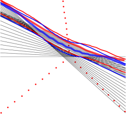
Figure 5.1: A set of thirty points, its dual, and the $12$ and $18$ levels. These two levels cannot be separated by a line, as the maximum Tukey depth is $10$ (realized by the centerpoint).

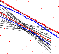
Figure 5.2: A set of $n=30$ random points, its dual, and the $12$ and $18$ levels. These two levels can be separated by a line, as the maximum Tukey depth is close to $n/2$ (see Remark 5.1).

Understanding this intersection polytope is somewhat easier in the dual. See Definition 2.1. Let $H_{\uparrow}$ (resp., $H_{\downarrow}$) be the set of all hyperplanes that bounds from below (resp., above) a halfspace which contains strictly more than $n-k$ points of $P$. A point $p\in\mathcal{T}_{k}$ lies above (resp., below) all the hyperplanes of $H_{\uparrow}$ (resp., $H_{\downarrow}$).

The dual of $H_{\uparrow}$ is the set of points $H^{\star}_{\uparrow}=\left\{h^{\star}\;\middle|\;h\in H_{\uparrow}\right\}$. As duality is order flipping (Fact 2.2), it follows that all the points of $H^{\star}_{\uparrow}$ lie (vertically) below the hyperplane $p^{\star}$. The set $H^{\star}_{\downarrow}$ is defined in a similar fashion, and the points of $H^{\star}_{\downarrow}$ lie above the hyperplane $p^{\star}$.

Specifically, a point $p=(p_{1},\ldots,p_{d})$ induces in the dual the hyperplane $p^{\star}$ with equation $x_{d}=-p_{d}+\sum_{i=1}^{d-1}x_{i}p_{i}$. The condition that a point $s\in H^{\star}_{\uparrow}$ lies below the hyperplane $p^{\star}$, then reduces to the linear inequality (the variables being the coordinates of $p$) that

$$s_{d}\leq-p_{d}+\sum_{i=1}^{d-1}s_{i}p_{i},$$

As such, computing a point in $\mathcal{T}_{k}$ is no more than solving a linear program when each point of $H^{\star}_{\uparrow}\cup H^{\star}_{\downarrow}$ induces a constraint. This LP computes a separating hyperplane between $H^{\star}_{\uparrow}$ and $H^{\star}_{\downarrow}$.

In the dual, the set of points $P$ becomes a set of hyperplanes $P^{\star}$. A hyperplane $h\in H_{\uparrow}$ in the dual is a point $h^{\star}$, such that there are at least $n-k$ hyperplanes of $P^{\star}$ strictly below it (in the $x_{d}$ direction). The number of such hyperplanes is the level of the point. The set $H_{\uparrow}$ is thus the set of all the points that have level strictly larger than $n-k$. The boundary of the closure of $H^{\star}_{\uparrow}$ (resp., $H^{\star}_{\downarrow}$) is the $(n-k)$-level (resp., $k$-level).

In two dimensions, these levels are $k$-monotone polygonal curves. The complexity of the $k$-level can be superlinear—a lower bound of $n2^{\Omega(\sqrt{\log k})}$ is known [Tót01], and currently the best upper bound is $O(nk^{1/3})$ [Dey98]. As such, finding if there is a point of Tukey depth $k$ is equivalent to deciding if there is a line that separates the $k$-level from the $(n-k)$-level. In higher dimensions these levels are surfaces, and one is looking for a hyperplane separating them.

In particular, this implies that to decide if there is a point of Tukey depth $k$, one can solve the LP defined in the dual to decide if the $k$-level and the $(n-k)$-level are linearly separable. In two dimensions, these two levels are polygonal curves, and it is enough to decide if their vertices are linearly separable. See Figure 5.1 and Figure 5.2.

Since the two levels can be computed in roughly $O(n^{4/3})$ time (and this also bounds the number of their vertices), and linear programming in two dimensions works in linear time, it follows that one can decide whether there is a point of Tukey depth $k$ in roughly $O(n^{4/3})$ time. To get a faster algorithm, we deploy our implicit LP algorithm. Intuitively, the new algorithm computes an approximation of the two levels, and thus computes a subset of the constraints of the explicit LP. The algorithm refines these approximations in such a way that the resulting rougher LP has a solution if and only if the original LP has the same solution.

5.1.2 The algorithm

To deploy our framework for implicit LP, we need a partition scheme and a verifier, which we provide next.

5.1.2.1 Partitioning scheme

A bundle $(H,\nabla,\tau)$ of constraints in the implicit LP (of separating the two levels), is a simplex $\nabla$, the subset

$$H=\left\{h\in P^{\star}\;\middle|\;h\cap\nabla\neq\emptyset\right\},$$

and a number $\tau$, which is the depth of a specific corner of $\nabla$ in the original arrangement $\mathcal{A}=\mathcal{A}\left({P^{\star}}\right)$. This bundle contains all the constraints that define points of the $k$- and $(n-k)$-level of $\mathcal{A}$ that lie in $\nabla$. More broadly, given the bundle, one can compute the arrangement $\mathcal{A}\cap\nabla$. Thus, with the information provided, one can compute the level of all the points inside $\nabla$ in $\mathcal{A}$ – one can compute $\mathcal{A}\cap\nabla$ and then propagate the depth information from the specific corner of $\nabla$.

A $(1/r)$-cutting restricted to the interior of $\nabla$ can be computed in $O(\left|{H}\right|r^{d-1})$ time, by Lemma 2.7. Each cell in the cutting is a new bundle. Computing the depth of a point on the boundary of each sub-simplex can be done easily in the same time bound. Each bundle has $\left|{H}\right|/r$ hyperplanes in its conflict list.

5.1.2.2 The verifier

Lemma 5.3.

Let $P^{\star}$ be a set of $n$ hyperplanes in $\mathbb{R}^{d}$, and let $t^{-},t^{+}$ be two numbers. Given a hyperplane $h$ one can decide in $O(n\log n+n^{d-1})$ time whether $h$ separates the $t^{-}$-level from the $t^{+}$-level of $\mathcal{A}=\mathcal{A}\left({P^{\star}}\right)$.

Proof:

Consider any hyperplane of $P^{\star}$ as bounding a halfspace that lies above it, and let $H$ be the resulting set of halfspaces. The depth of a point $p$ is the number of halfspaces of $H$ that contain $p$, and is the level of the point in the arrangement $\mathcal{A}$. Thus, it is enough to compute the range of depths realized by points lying on $h$. The intersection of each $d$-dimensional halfspace of $H$ with $h$ is a $(d-1)$-dimensional halfspace of $h$. This range of depths can be computed by computing the arrangement of these $n$ induced halfspaces on the hyperplane $h$. As $h$ is $(d-1)$-dimensional, this requires $O(n\log n)$ time if $d=2$ (via essentially sorting), and $O(n^{d-1})$ in higher dimensions.

Specifically, the algorithm computes for each face of the arrangement on $h$ its depth, which results in the range of depths of points on $h$. If the range lies outside $[t^{-},t^{+}]$ then $h$ is not the desired separating hyperplane.  

Consider a bundle $(H,\nabla,\tau)$. Here, the algorithm maintains the set $H\cap\nabla$, and a corner $p$ of $\nabla$, such that its level is $\tau$. One can compute the range of levels realized on the faces of $\nabla$ using Lemma 5.3. Since the level of a point is monotone increasing along a vertical line, it follows that this provides the range of levels realized also by the interior of $\nabla$.

Given a hyperplane $h$, one needs to verify if it is feasible for this bundle. To this end, one can first check if it intersects $\nabla$. If not, then the computed range of levels realized in $\nabla$ is sufficient to decide if it is feasible as far as the levels inside $\nabla$. Otherwise, the algorithm computes the level of some point $s\in\nabla\cap h$, by computing how the level changes as one moves from $p$ to $s$ (as we know the level of $p$, and as $ps$ can intersect only hyperplanes in the set $H\cap\nabla$). Now, using Lemma 5.3 one can compute the range of levels encountered on $\nabla\cap h$, which is sufficient to verify whether $h$ separates the desired levels inside $\nabla$. Note that if $m=\left|{H\cap\nabla}\right|$, then the running time of this algorithm is $O(m\log m+m^{d-1})$.

5.1.2.3 Putting everything together

We next deploy the algorithm of Theorem 4.5. In the dual, we are solving an LP computing a hyperplane separating the $k$ level from the $(n-k)$ level. To this end, we pick an arbitrary linear constraint on the LP that we are trying to (say) minimize. We sketched a verifier, and a partitioning schemes, that for $n$ hyperplanes, work in $\mathcal{D}\left({n}\right)=O(n\log n+n^{d-1})$ time. We thus get the following.

Theorem 5.4.

Let $P$ be a set of $n$ points in $\mathbb{R}^{d}$, and let $k$ be a parameter. One can compute a point in $\mathbb{R}^{d}$ of Tukey depth at least $k$, if such a point exists, in $O(n\log n+n^{d-1})$ expected time.

5.1.3 Computing a point of maximum Tukey depth

Having solved the problem of deciding whether the maximum Tukey depth is at least $k$, we consider the problem of computing the maximum Tukey depth. Using binary search on top of Theorem 5.4 one can compute a point with maximum Tukey depth (paying an extra log factor). However, one can do better by considering the associated ranking LP problem (described in Section 3.1).

For a vertex $p$ of $\mathcal{A}\left({P^{\star}}\right)$, its associated rank is $\mathrm{r}\left({p}\right)=|n/2-\mathrm{level}\left({p}\right)|$. The LP ranking problem, with all the vertices of $\mathcal{A}\left({P^{\star}}\right)$ as constraints, is exactly the problem of finding a point of maximum Tukey depth. By Lemma 3.1 this is an LP-type problem. The idea is now to solve this implicit LP using the above machinery.

A basis now is a set of $d+1$ vertices of $\mathcal{A}\left({P^{\star}}\right)$. It is easy to modify the algorithm, for solving this implicit ranking LP problem, so that it explicitly computes the level of each vertex/constraint being considered. As such, the rank of the basis is known. Now, such a basis defines a separating hyperplane and it is supposed to separate specific levels as defined by its rank. Thus, the active constraints are induced by the points on these active levels. Clearly, the verifier above works (unmodified) for this case, as does the partition scheme. We thus get the following.

Theorem 5.5.

Let $P$ be a set of $n$ points in $\mathbb{R}^{d}$. One can compute a point in $\mathbb{R}^{d}$ of maximum Tukey depth, in $O(n\log n+n^{d-1})$ expected time.

5.1.4 Computing a depth region in two dimensions

In two dimensions, our approach can speed up an existing algorithm by Matoušek [Mat90] for computing the entire region of depth $\geq k$ (i.e., the convex polytope $\mathcal{T}_{k}$ in Lemma 5.2). The $O(n\log^{4}n)$ time bound is improved to $O(n\log^{2}n)$.

Theorem 5.6.

Let $P$ be a set of $n$ points in $\mathbb{R}^{2}$, and let $k$ be a parameter. One can compute the region $\mathcal{T}_{k}$ of all points in $\mathbb{R}^{d}$ of Tukey depth at least $k$ in $O(n\log^{2}n)$ expected time.

Proof:

Matoušek [Mat90] noted that the problem reduces to computing the upper hull of the $k$-level in the dual plane. He described a divide-and-conquer algorithm to compute this “level hull”, using an oracle for the following subproblem: given a set of $n$ lines in the plane, a number $k$, and a vertical line $\ell$, find the tangent of the upper hull at $\ell$. He applied a two-level parametric search to solve this subproblem in $O(n\log^{3}n)$ time. By our approach, we can solve this subproblem in $O(n\log n)$ expected time: back in primal space, the subproblem is equivalent to finding a point in the region $\mathcal{T}_{k}$ that maximizes a given linear function. This is an implicit LP problem, and the method in this section yields an $O(n\log n)$-time randomized algorithm.

The overall running time of Matoušek’s divide-and-conquer algorithm is bounded by a logarithmic factor times the running time of the oracle, and is thus $O(n\log^{2}n)$.  

6 The extremal yolk as an implicit LP

6.1 Background

Definition 6.1.

Let $P\subset\mathbb{R}^{d}$ be a set of $n$ points in general position. A median hyperplane is a hyperplane such that each of its two closed halfspaces contain at least $\left\lceil{n/2}\right\rceil$ points of $P$. A hyperplane is extremal if it passes through $d$ points of $P$. The extremal yolk is the ball of smallest radius interesting all extremal median hyperplanes of $P$.

We give an $O(n^{d-1}\log n)$ expected time exact algorithm computing the extremal yolk. To do so, we focus on the more general problem.

Problem 6.2.

Let $E_{k}(P)$ be the collection of extremal hyperplanes which contain exactly $k$ points of $P$ on or above them. Here, $k$ is not necessarily constant. The goal is to compute the smallest radius ball intersecting all hyperplanes of $E_{k}(P)$.

We observe that computing the extremal yolk can be reduced to the above problem.

Lemma 6.3.

The problem of computing the extremal yolk can be reduced to Problem 6.2.

Proof:

Suppose that $n$ is even, and define the set $S_{\textup{even}}=\{n/2,n/2+1,\ldots,n/2+d\}$. A case analysis shows that any extremal median hyperplane $h$ must have exactly $m$ points of $P$ above or on $h$, where $m\in S_{\textup{even}}$. Thus, computing the extremal yolk reduces to computing smallest radius ball intersecting all hyperplanes in the set $\bigcup_{m\in S_{\textup{even}}}E_{m}(P)$.

When $n$ is odd, a similar case analysis shows that any extremal median hyperplane must have exactly $m$ points above or on it, where $m\in S_{\textup{odd}}=\{\left\lceil{n/2}\right\rceil,\left\lceil{n/2}\right\rceil+1,\ldots,\left\lceil{n/2}\right\rceil+d-1\}$. Analogously, computing the extremal yolk with $n$ odd reduces to computing the smallest radius ball intersecting all hyperplanes in the set $\bigcup_{m\in S_{\textup{odd}}}E_{m}(P)$.  

We use Theorem 4.5 to solve Problem 6.2. To this end, we prove that Problem 6.2 is an LP-type problem when the constraints are explicitly given (the following Lemma was also observed by Bhattacharya et al. [BJMR94]).

Lemma 6.4.

Problem 6.2 when the constraints (i.e., hyperplanes) are explicitly given is an LP-type problem and has combinatorial dimension $\delta=d+1$.

Proof:

We prove something stronger, namely that the problem can be written as a linear program, implying it is an LP-type problem. Let ${H}$ be the set of $n$ hyperplanes. For each hyperplane $h\in{H}$, let $\left\langle{a_{h},x}\right\rangle+b_{h}=0$ be the equation describing $h$, where $a_{h}\in\mathbb{R}^{d}$, $\left\|{a_{h}}\right\|=1$, and $b_{h}\in\mathbb{R}$. Because of the requirement that $\left\|{a_{h}}\right\|=1$, for a given point $p\in\mathbb{R}^{d}$, the distance from $p$ to a hyperplane $h$ is $\left|{\left\langle{a_{h},p}\right\rangle+b_{h}}\right|$.

The linear program has $d+1$ variables and $2n$ constraints. The $d+1$ variables represent the center $p\in\mathbb{R}^{d}$ and radius $\nu\geq 0$ of the egg. The resulting LP is

min $$\nu$$

subject to $$\nu\geq\left\langle{a_{h},p}\right\rangle+b_{h} \forall h\in{H}$$

$$\nu\geq-\bigl{(}\left\langle{a_{h},p}\right\rangle+b_{h}\bigr{)} \forall h\in{H}$$

$$p\in\mathbb{R}^{d}.$$

As for the combinatorial dimension, observe that any basic feasible solution for the above linear program will be tight for at most $d+1$ of the above $2n$ constraints. Namely, these $d+1$ hyperplanes are tangent to the optimal radius ball, and as such form a basis $\mathcalb{b}\subseteq{H}$.  

To apply Theorem 4.5 we need to: (i) design an appropriate input space, (ii) develop a decider, and (iii) construct a constant number of subproblems which cover the constraint space. As in Section 5, the algorithm works in the dual space. The following lemma shows that the dual of a ball $\mathsf{b}$ is the closed region which lies between two branches of a hyperboloid. See Figure 6.1.

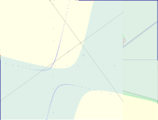
Figure 6.1: A disk and its dual.

Lemma 6.5.

The dual of the set of points in a ball is the set of hyperplanes whose union forms the region enclosed between two branches of a hyperboloid.

Proof:

In $\mathbb{R}^{d}$ the hyperplane $h$ defined by $x_{d}=\beta+\sum_{i=1}^{d-1}\alpha_{i}x_{i}$, or more compactly $\left\langle{x,(-\alpha,1)}\right\rangle=\beta$, intersects a disk $\mathsf{b}$ centered at $p=(p_{1},\ldots,p_{d})$ with radius $r$ $\iff$ the distance of $h$ from $p$ is at most $r$. That is, $h$ intersects $\mathsf{b}$ if

$$\frac{\left|{\left\langle{p,(-\alpha,1)}\right\rangle-\beta}\right|}{\left\|{(-\alpha,1)}\right\|}\leq r \iff\left({\left\langle{p,(-\alpha,1)}\right\rangle-\beta}\right)^{2}\leq r^{2}\left\|{(-\alpha,1)}\right\|^{2}$$

$$\iff\Bigl{(}p_{d}-\beta-\sum_{i=1}^{d-1}\alpha_{i}p_{i}\Bigr{)}^{2}\leq r^{2}(\left\|{\alpha}\right\|^{2}+1).$$

$$\iff\frac{\bigl{(}p_{d}-\beta-\sum_{i=1}^{d-1}\alpha_{i}p_{i}\bigr{)}^{2}}{r^{2}}-\left\|{\alpha}\right\|^{2}\leq 1.$$

The boundary of the above inequality is a hyperboloid in the variables $p_{d}-\beta-\sum_{i=1}^{d-1}\alpha_{i}p_{i}$ and $\alpha_{1},\ldots,\alpha_{d-1}$. This corresponds to an affine image of a hyperboloid in the dual space $\alpha\times-\beta$.  

Throughout, let $\mathsf{b}^{\star}$ denote the region between the two branches of the hyperboloid dual to a ball $\mathsf{b}$.

6.2 Solving the subproblem

We verify the requirements of Theorem 4.5 can be met. First, we develop the algorithm for the violation test. As the algorithm works in the dual, each subproblem consists of a simplex $\Delta$, the dual set of hyperplanes $H=P^{\star}\cap\Delta$ intersecting $\Delta$, and a parameter $\mathsf{u}$ which is the number of hyperplanes lying completely below $\Delta$. Additionally, the given basis defines a ball $\mathsf{b}$, which in the dual is the region $\mathsf{b}^{\star}$. One can verify in the dual, that the violation test must decide if there is a vertex of the $k$-level in the region $\mathbb{R}^{d}\setminus\mathsf{b}^{\star}$.

Lemma 6.6.

Given the input $(H,\Delta,\mathsf{u})$ and the region $\mathsf{b}^{\star}$, checking whether there is a vertex of $\mathcal{A}\left({H}\right)$ which has level $k$ and lies inside $\mathbb{R}^{d}\setminus\mathsf{b}^{\star}$ can be done in $O(n^{d-1}\log n)$ time.

Proof:

Observe that $\Delta\cap(\mathbb{R}^{d}\setminus\mathsf{b}^{\star})$ is the union of at most two convex regions. Indeed, the set $\mathbb{R}^{d}\setminus\mathsf{b}^{\star}$ consists of two disjoint connected components, where each component is a convex body. Intersecting a simplex $\Delta$ with each component of $\mathbb{R}^{d}\setminus\mathsf{b}^{\star}$ produces two (disjoint) convex bodies $\Delta^{\prime}$ and $\Delta^{\prime\prime}$ (it is possible that $\Delta^{\prime}$ or $\Delta^{\prime\prime}$ are empty). See Figure 6.2. Let $\Delta^{\prime}$ be one of these two regions of interest. The algorithm will process $\Delta^{\prime\prime}$ in exactly the same way.

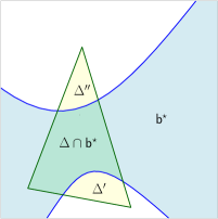
Figure 6.2: The region $\Delta\cap(\mathbb{R}^{d}\setminus\mathsf{b}^{\star})$ consists of (at most) two disjoint convex regions, $\Delta^{\prime}$ and $\Delta^{\prime\prime}$.

If $\Delta^{\prime}$ is empty, then no constraints are violated. Otherwise, we need to check for any violated constraints inside $\Delta^{\prime}$. Let $\partial\Delta^{\prime}$ denote the boundary of $\Delta^{\prime}$. Define $H^{\prime}\subseteq H$ to be the subset of hyperplanes intersecting $\Delta^{\prime}$. Observe that it suffices to check if there is a vertex $v$ in the arrangement $\mathcal{A}\left({H^{\prime}}\right)$ such that: (i) $v$has level $k$ in $P^{\star}$, (ii) $v$is a member of some cell in the zone $\mathcal{Z}\left({\partial\Delta^{\prime},H^{\prime}}\right)$, and (iii) $v$is contained in $\Delta^{\prime}$.

The algorithm computes $\mathcal{Z}\left({\partial\Delta^{\prime},H^{\prime}}\right)$. Next, it chooses a vertex $v$ of the arrangement $\mathcal{A}\left({H^{\prime}}\right)$ which lies inside $\Delta^{\prime}$ and computes its level in $H^{\prime}$ (adding $\mathsf{u}$ to the count). The algorithm then walks around the vertices of the zone inside $\Delta^{\prime}$, computing the level of each vertex along the walk. Note that the level between any two adjacent vertices in the arrangement differ by at most a constant (depending on $d$). If at any point we find a vertex of the desired level (such a vertex also lies inside $\Delta^{\prime}$), we report the corresponding median hyperplane which violates the given ball $\mathsf{b}$. See Figure 6.3 for an illustration.

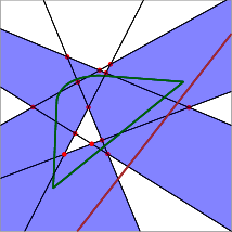
Figure 6.3: Left: A convex region $\Delta^{\prime}$, with one line lying completely below $\Delta^{\prime}$ ($\mathsf{u}=1$). The shaded regions are the cells of $\mathcal{Z}\left({\partial\Delta^{\prime},H^{\prime}}\right)$. The vertices of the cells in the zone $\mathcal{Z}\left({\partial\Delta^{\prime},H^{\prime}}\right)$ are highlighted. Right: The vertices of $\mathcal{Z}\left({\partial\Delta^{\prime},H^{\prime}}\right)$ which are part of the 3-level and contained inside $\Delta^{\prime}$.

The running time of the algorithm is proportional to the complexity of the zone $\mathcal{Z}\left({\partial\Delta^{\prime},H^{\prime}}\right)$. Because the boundary of $\Delta^{\prime}$ is constructed from $d+1$ hyperplanes and the boundary of the hyperboloid, Lemma 2.5 implies that the zone complexity is no more than $O(\left|{H}\right|^{d-1}\log\left|{H}\right|)$. As such, the algorithm runs in time $\mathcal{D}\left({n}\right)=O(n^{d-1}\log n)$.  

Lemma 6.7.

Let $P\subset\mathbb{R}^{d}$ be a set of $n$ points in general position. For a given integer $k$, one can compute in $O(n^{d-1}\log n)$ expected time the smallest radius ball intersecting all of the hyperplanes of $E_{k}(P)$

Proof:

Apply Theorem 4.5. The violation test follows from Lemma 6.6. Constructing the subproblems from a given input $(H,\Delta,\mathsf{u})$ is done in the same way as Theorem 5.4. Compute a $(1/c)$-cutting (for constant $c$ sufficiently large) of $H$ and clip the cutting inside $\Delta$. For each cell $\Delta_{i}$ in the cutting, compute $H_{i}=P^{\star}\cap\Delta_{i}$ and the parameter $\mathsf{u}_{i}$. This entire step can be performed in linear time. Hence, the problem can be solved in $O(\mathcal{D}\left({n}\right))$ expected time, where $\mathcal{D}\left({n}\right)=O(n^{d-1}\log n)$.  

Corollary 6.8.

Let $P\subset\mathbb{R}^{d}$ be a set of $n$ points in general position, and let $S\subseteq\left\llbracket n\right\rrbracket$. One can compute in $O(n^{d-1}\log n)$ expected time the smallest radius ball intersecting all of the hyperplanes of $\bigcup_{k\in S}E_{k}(P)$.

Proof:

The algorithm is a slight modification of Lemma 6.7. During the decision procedure, for each vertex in the zone, we check if it is a member of the $k$-level for some $k\in S$. If $S$ is of non-constant size, membership in $S$ can be checked in constant time using hashing.  

6.3 Computing the extremal yolk and the egg

Theorem 6.9.

Let $P\subset\mathbb{R}^{d}$ be a set of $n$ points in general position. One can compute the extremal yolk of $P$ in $O(n^{d-1}\log n)$ expected time.

Proof:

The result follows by applying Corollary 6.8 with the appropriate choice of $S$. When $n$ is even, Lemma 6.3 tells us to choose $S=\{n/2,n/2+1,\ldots,n/2+d\}$. When $n$ is odd, we set $S=\{\left\lceil{n/2}\right\rceil,\left\lceil{n/2}\right\rceil+1,\ldots,\left\lceil{n/2}\right\rceil+d-1\}$.  

Lemma 6.10.

Let $P\subset\mathbb{R}^{d}$ be a set of $n$ points in general position. One can compute the egg of $P$ in $O(n^{d-1}\log n)$ expected time.

Proof:

The proof follows by Corollary 6.8 with $S=\left\llbracket n\right\rrbracket$. (Alternatively, by directly modifying the decision procedure to check if any vertex of the zone $\mathcal{Z}\left({\Delta^{\prime},H^{\prime}}\right)$ lies inside $\Delta^{\prime}$.)  

6.4 An algorithm sensitive to $k$

Here, we solve Problem 6.2 for the case that $k\ll n$. Recall that to compute the extremal yolk, we reduced the problem to computing the smallest ball intersecting all hyperplanes which contain a fixed number of points of $P$ above or on them (see Lemma 6.3). In particular, we developed an algorithm for Problem 6.2 and applied it when $k$ is proportional to $n$.

To develop an algorithm sensitive to $k$, we use the result of Lemma 6.7 as a black box and introduce the notion of shallow cuttings.

Definition 6.11 (Shallow cuttings).

Let $H$ be a set of $n$ hyperplanes in $\mathbb{R}^{d}$. A $k$-shallow cutting is a collection of simplices such that: (i) the union of the simplices covers the $(\leq k)$-level of $H$ (see Definition 2.3), and (ii) each simplex intersects at most $k$ hyperplanes of $H$.

Matoušek was the first to provide an algorithm for computing $k$-shallow cuttings of size $O((n/k)^{\left\lfloor{d/2}\right\rfloor})$ [Mat92]. When $d=2,3$, a $k$-shallow cutting of size $O(n/k)$ can be constructed in $O(n\log n)$ time [CT16]. For $d\geq 4$, we sketch a randomized algorithm which computes a $k$-shallow cutting, based on Matoušek’s original proof of existence [Mat92].

Lemma 6.12 (Proof sketch in Appendix A).

Let $H$ be a set of $n$ hyperplanes in $\mathbb{R}^{d}$. A $k$-shallow cutting of size $O((n/k)^{\left\lfloor{d/2}\right\rfloor})$ can be constructed in $O(k(n/k)^{\left\lfloor{d/2}\right\rfloor}+n\log n)$ expected time. For each simplex $\Delta$ in the cutting, the algorithm returns the set of hyperplanes intersecting $\Delta$ and the number of hyperplanes lying below $\Delta$.

Let $P\subset\mathbb{R}^{d}$ be a set of $n$ points and let $H=P^{\star}$ be the set of dual hyperplanes. The algorithm first computes a $k$-shallow cutting for the top and bottom $(\leq k)$-levels for the given set of hyperplanes $H$ using Lemma 6.12. Let $\Delta_{1},\ldots,\Delta_{\ell}$, where

$$\ell=O((n/k)^{\left\lfloor{d/2}\right\rfloor}),$$

be the collection of simplices in the cutting. For each simplex $\Delta_{i}$, we have the subset $H\cap\Delta_{i}$ and the number of hyperplanes lying completely below $H$ (which is at most $k$). For each cell $\Delta_{i}$, let $g(\Delta_{i})$ be the set of vertices of $\mathcal{A}\left({H}\right)$ which have level $k$ or $n-k$ and are contained in $\Delta_{i}$.

6.4.1 The algorithm

The algorithm computes the above shallow cutting, and treats each simplex as a bundle. We now apply the algorithm of Section 3.3 to solve the batched LP problem defined by these bundles, except that we delegate each basis calculation/verification to a call to the algorithm of Lemma 6.7, which involves a single bundle (i.e., $k$ hyperplanes).

Lemma 6.13.

Let $P\subset\mathbb{R}^{d}$ be a set of $n$ points in general position. For a given integer $k$, one can compute in $O\left({k^{d-1}\big{(}1+(n/k)^{\left\lfloor{d/2}\right\rfloor}\big{)}\log k+n\log n}\right)$ expected time the smallest radius ball intersecting all of the hyperplanes of $E_{k}(P)$.

Proof:

The algorithm is described above. The correctness is immediate from Lemma 3.5. As for the running time, the algorithm performs $O(\ell)$ basis calculations and violation tests, and each one takes $O(k^{d-1}\log k)$ time, as this is the size of the conflict list of each bundle. This running time dominates the time to compute the cutting, except for the $O(n\log n)$ additive term.  

7 The (continuous) yolk as an implicit LP

7.1 Background

Definition 7.1.

Let $P\subset\mathbb{R}^{d}$ be a set of $n$ points in general position. The continuous yolk of $P$ is the ball of smallest radius intersecting all median hyperplanes of $P$.

In contrast to Definition 6.1, we emphasize that the (continuous) yolk must intersect all median hyperplanes defined by $P$ (not just extremal median hyperplanes).

As before, the algorithm works in the dual space. For an integer $k$, let $H_{k}(P)$ be the collection of halfspaces containing exactly $k$ points of $P$ on or above it. Equivalently, $P^{\star}$ is the collection of hyperplanes defined by $P$ in the dual space, and $\bigl{(}H_{k}(P)\bigr{)}^{\star}$ is the $k$-level of $P^{\star}$. Our problem can be restated in the dual space as follows.

Problem 7.2.

Let $P$ be a set of points in $\mathbb{R}^{d}$ in general position and let $k$ be a given integer. Compute the ball $\mathsf{b}$ of smallest radius so that all points in the $k$-level of $P^{\star}$ are contained inside the region $\mathsf{b}^{\star}$.

Let $L_{k}(P)=\bigl{(}H_{k}(P)\bigr{)}^{\star}$ denote the set of all points in the $k$-level of $P^{\star}$. Note that $L_{k}(P)$ consists of points which are either contained in the interior of some $\ell$-dimensional flat, where $0\leq\ell\leq d-1$, or in the interior of some $d$-dimensional cell of $\mathcal{A}\left({P^{\star}}\right)$.

We take the same approach as the algorithm of Theorem 6.9—building a decider subroutine, and showing that the input space can be decomposed into subproblems efficiently. However the problem is more subtle, as the collection of constraints (i.e., median hyperplanes) is no longer a finite set.

7.1.1 The input space

The input consists of a simplex $\Delta$. The algorithm, in addition to $\Delta$, maintains the set of hyperplanes

$$H=P^{\star}\cap\Delta=\left\{h\in P^{\star}\;\middle|\;h\cap\Delta\neq\emptyset\right\},$$

and a parameter $\mathsf{u}$ which is equal to the number of hyperplanes of $P^{\star}$ lying completely below $\Delta$.

7.1.2 The implicit constraint space

Each input $\Delta$ maps to a region $R$ which is the portion of the $k$-level $L_{k}(P)$ contained inside $\Delta$. For each $d$-dimensional cell in $R$, we compute its bottom-vertex triangulation (see, e.g., [Mat02, Section 6.5]), and collect all of these simplices, and all lower-dimensional faces of $R$, into a set $g(\Delta)$. See Figure 7.1.

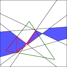
Figure 7.1: Left: A set of lines and the cells of the $3$-level. Middle: A simplex $\Delta$, with the portion of the $3$-level inside $\Delta$. Right: Triangulating the portion of the $3$-level contained inside $\Delta$. All red triangles together with the lower-dimensional faces of the $3$-level form the set of constraints $g(\Delta)$.

Let $\Xi$ be the collection of all simplices formed from $d+1$ vertices of the arrangement $\mathcal{A}\left({P^{\star}}\right)$. We let ${H}$ be the union of the sets $g(\Delta)$ over all simplices $\Delta\in\Xi$. To see why this suffices, each simplex in the input space is a simplex generated by a cutting algorithm. One property of cutting algorithms [Cha93] is that the simplices returned are induced by hyperplanes of $P^{\star}$. Indeed, each simplex has (at most) $d+1$ vertices, and upon inspection of the cutting algorithm, each vertex is defined by $d$ hyperplanes of $P^{\star}$. There are a finite number of simplices $\Delta$ to consider, and each $\Delta$ induces a fixed subset of constraints $g(\Delta)\subseteq{H}$.

As such, ${H}$ forms our constraint set, where each constraint is of constant size (depending on $d$). Clearly, a solution satisfies all constraints of ${H}$ if and only if the solution intersects all hyperplanes in the set $H_{k}(P)$. For a given subset $\mathcal{C}\subseteq{H}$, the objective function is the minimum radius ball $\mathsf{b}$ such that all regions of $\mathcal{C}$ are contained inside the region $\mathsf{b}^{\star}$. In particular, the problem of computing the minimum radius ball $\mathsf{b}$ such that $\mathsf{b}^{\star}$ contains all points of $L_{k}(P)$ in its interior is an LP-type problem of constant combinatorial dimension.

7.2 The algorithm

7.2.1 Constructing subproblems

For a given input simplex $\Delta$ (along with the set $H=P^{\star}\cap\Delta$ and the number $\mathsf{u}$) a collection of subproblems $\Delta_{1},\ldots,\Delta_{\psi}$ (with the corresponding sets $H_{i}$ and numbers $\mathsf{u}_{i}$ for $i=1,\ldots,\psi$) can be constructed as described in Lemma 6.7, by computing a cutting of the planes $H$ and clipping this cutting inside $\Delta$. In particular, we have that $\bigcup_{i}g(\Delta_{i})=g(\Delta)$. Strictly speaking, we have not decomposed the constraints of $g(\Delta)$ (as required by Theorem 4.5), but rather have decomposed the region which is the union of the constraints of $g(\Delta)$. This step is valid, as a solution satisfies the constraints of $\bigcup_{i}g(\Delta_{i})$ if and only if it satisfies the constraints of $g(\Delta)$.

7.2.2 The decision procedure

Given a candidate solution $\mathsf{b}^{\star}$, the problem is to decide if $\mathsf{b}^{\star}$ contains $g(\Delta)$ in its interior. The decision algorithm itself is similar as in the proof of Theorem 6.9. Consider the set $\Delta\cap(\mathbb{R}^{d}\setminus\mathsf{b}^{\star})$, where $\Delta$ is a simplex, and observe that it is the union of at most two convex regions. Let $\Delta^{\prime}$ be one of these two regions of interest. Observe that it suffices to check if there is a point on the boundary of $\Delta^{\prime}$ which is part of the $k$-level. Let $H^{\prime}\subseteq H$ be the subset of hyperplanes intersecting $\Delta^{\prime}$.

To this end, compute $\mathcal{Z}\left({\partial\Delta^{\prime},H^{\prime}}\right)$. For each $(d-1)$-dimensional face $f$ of $\Delta^{\prime}$, the collection of regions $\Xi=\left\{f\cap s\;\middle|\;s\in\mathcal{Z}\left({\partial\Delta^{\prime},H^{\prime}}\right)\right\}$ forms a $(d-1)$-dimensional arrangement restricted to $f$. Furthermore, the complexity of this arrangement lying on $f$ is at most $O(n^{d-1}\log n)$. Notice that the level of all points in the interior of a face of $\Xi$ is constant, and two adjacent faces (sharing a boundary) have their level differ by at most a constant. The algorithm picks a face in $\Xi$, computes the level of an arbitrary point inside it (adding $\mathsf{u}$ to the count). Then, the algorithm walks around the arrangement, exploring all faces, using the level of neighboring faces to compute the level of the current face. If at any step a face has level $k$, we report that the input $(\Delta,H,\mathsf{u})$ violates the candidate solution $\mathsf{b}^{\star}$.

7.2.2.1 Analysis of the decision procedure

We claim the running time of the algorithm is proportional to the complexity of the zone $\mathcal{Z}\left({\partial\Delta^{\prime},H^{\prime}}\right)$. Indeed, for each $(d-1)$-dimensional face $f$ of $\Delta^{\prime}$ (where $f$ may either be part of a hyperplane or part of the boundary of $\mathsf{b}^{\star}$), we can compute the set $\left\{f\cap s\;\middle|\;s\in\mathcal{Z}\left({\partial\Delta^{\prime},H^{\prime}}\right)\right\}$ in time proportional to the total complexity of $\mathcal{Z}\left({\partial\Delta^{\prime},H^{\prime}}\right)$ (assuming we can intersect a hyperplane with a portion of a constant-degree surface efficiently). The algorithm then computes the level of an initial face naively in $O(\left|{H^{\prime}}\right|)$ time, and computing the level of all other faces can be done in $O(\left|{\mathcal{Z}\left({\partial\Delta^{\prime},H^{\prime}}\right)}\right|)$ time by performing a graph search on the arrangement.

Because the boundary of $\Delta^{\prime}$ is constructed from $d+1$ hyperplanes and the boundary of the hyperboloid, Lemma 2.5 implies that the zone complexity is bounded by $O(\left|{H}\right|^{d-1}\log\left|{H}\right|)$. As such, our decision procedure runs in time $\mathcal{D}\left({n}\right)=O(n^{d-1}\log n)$.

7.2.2.2 A slightly improved decision procedure

In $\mathbb{R}^{3}$, one can shave the $O(\log n)$ factor to obtain an $O(n^{2})$ expected time algorithm. We modify the decision procedure as follows, which avoids computing the zone $\mathcal{Z}\left({\partial\Delta^{\prime},H^{\prime}}\right)$. For each 2D face $f$ of $\Delta^{\prime}$, simply compute the arrangement of the set of curves $\left\{f\cap h\;\middle|\;h\in H\right\}$ on $f$ in $O(n^{2})$ time. As before, we perform a graph search on this arrangement, computing the level of each face. If at any time we discover a point on the boundary of $\Delta^{\prime}$, of the desired level, we report that the given input violates the given candidate solution.

For higher dimensions $d\geq 4$, we can similarly avoid computing the zone. Recall that the goal is to find a point $p$ that lies in the intersection of the $k$-level with a $(d-1)$-dimensional face $f$ of $\Delta^{\prime}$. Consider the (unknown) cell $\gamma$ containing $p$ in the arrangement of $\left\{f\cap h\;\middle|\;h\in H\right\}$ on $f$. Imagine moving $p$ to lie in an arbitrarily small neighborhood of the minimum point $p^{\prime}$ in $\gamma$ with respect to the $x_{d}$ coordinate. The level of $p$ remains unchanged by the move (and differs from the level of $p^{\prime}$ by at most $d$).

• Case 1: $p^{\prime}$ is incident to at most $d-2$ hyperplanes in $H$. We can search for such a $p^{\prime}$, by trying all tuples of at most $d-2$ hyperplanes. For each such tuple $(h_{1},\ldots,h_{\ell})$ with $\ell\leq d-2$, we compute all $O(1)$ local $x_{d}$-minima $q$ of $f\cap h_{1}\cap\ldots\cap h_{\ell}$. Next, we compute the level of $q$ naively in $O(n)$ time. Finally, we examine the neighborhood of $q$. This takes $O(n^{d-2}\cdot n)=O(n^{d-1})$ time.

• Case 2: $p^{\prime}$ is incident to $d-1$ hyperplanes in $H$. We try all tuples of $d-3$ hyperplanes. For each such tuple $(h_{1},\ldots,h_{d-3})$, we compute the two-dimensional arrangement of the set of curves

  $$\left\{f\cap h_{1}\cap\ldots\cap h_{d-3}\cap h\;\middle|\;h\in H\right\}$$

  on the two-dimensional surface $h_{1}\cap\ldots\cap h_{d-3}\cap f$ in $O(n^{2})$ time. As above, we perform a graph search on this arrangement, computing the level of each cell and each vertex in the arrangement, and examine the neighborhood of each vertex. The total time is $O(n^{d-3}\cdot n^{2})=O(n^{d-1})$.

Thus, our improved decision procedure runs in time $\mathcal{D}\left({n}\right)=O(n^{d-1})$ for any $d\geq 3$.

Lemma 7.3.

Problem 7.2 can be solved in $O(n\log n+n^{d-1})$ expected time, where $n=\left|{P}\right|$.

Proof:

Follows by plugging the above discussion into Theorem 4.5.  

By modifying the decision procedure appropriately, we also obtain a similar result to Corollary 6.8.

Corollary 7.4.

Let $P\subset\mathbb{R}^{d}$ be a set of $n$ points in general position, and let $S\subset\left\llbracket n\right\rrbracket$. The smallest ball intersecting all hyperplanes in $\bigcup_{k\in S}H_{k}(P)$ can be computed in $O(n\log n+n^{d-1})$ expected time.

Theorem 7.5.

Let $P\subset\mathbb{R}^{d}$ be a set of $n$ points in general position. One can compute the yolk of $P$ in $O(n\log n+n^{d-1})$ expected time.

Proof:

The result follows by applying Corollary 7.4 with the appropriate choice of $S$. When $n$ is even, Lemma 6.3 tells us to choose $S=\{n/2,n/2+1,\ldots,n/2+d\}$. When $n$ is odd, we set $S=\{\left\lceil{n/2}\right\rceil,\left\lceil{n/2}\right\rceil+1,\ldots,\left\lceil{n/2}\right\rceil+d-1\}$.  

8 The Tukey ball and center ball as implicit LPs

Here, we are dealing with an extension of Tukey depth (Definition 1.1). The set of all points with Tukey depth $\geq k$ is the polytope $\mathcal{T}_{k}$ (see Lemma 5.2). Recall that by the centerpoint theorem $\mathcal{T}_{n/(d+)}$ is not empty.

Definition 8.1.

Let $P\subset\mathbb{R}^{d}$ be a set of $n$ points in general position. For a parameter $k\leq n$, the Tukey ball of $P$ is the smallest radius ball intersecting halfspaces in the set $H_{k}(P)$.

The Tukey median is a point in $\mathbb{R}^{d}$ with maximum Tukey depth. If the Tukey median of $P$ has Tukey depth $k(P)$, then for $k>k(P)$ the set $\mathcal{T}_{k}$ is empty—the Tukey ball has non-zero radius. When $k\leq k(P)$, $\mathcal{T}_{k}$ is non-empty, implying that the Tukey ball has radius zero.

Definition 8.2.

Let $P\subset\mathbb{R}^{d}$ be a set of $n$ points in general position. For a parameter $k\leq k(P)$, the center ball of $P$ is the ball of largest radius contained in the region $\mathcal{T}_{k}$.

Recently, Oh and Ahn [OA19] develop an $O(n^{2}\log^{4}n)$ time algorithm for computing the polytope $\mathcal{T}_{k}$ in $\mathbb{R}^{3}$. In contrast, the center ball is the largest ball contained inside $\mathcal{T}_{k}$, and we show it can be computed in expected time $O(n^{2}\log n)$.

8.1 The Tukey ball in the dual

For a set of $n$ points $P$ in general position, it suffices to restrict our attention to hyperplanes which contain $d$ points of $P$, and one of the open halfspaces contains more than $n-k$ points of $P$. In the dual, each point $p\in P$ is mapped to a hyperplane $p^{\star}$ (see Definition 2.1). A hyperplane $h$ passing through $d$ points of $P$ maps to a point $h^{\star}$ which is a vertex in the arrangement $\mathcal{A}\left({P^{\star}}\right)$.

Recall that by Lemma 6.5, a ball $\mathsf{b}$ in the primal maps to the region enclosed by two branches of a hyperboloid. Formally, the region $\mathsf{b}^{\star}$ is the collection of points $(x_{1},\ldots,x_{d})\in\mathbb{R}^{d}$ satisfying has the equation $(x_{d}/\alpha_{d})^{2}-\sum_{i=1}^{d-1}(x_{i}/\alpha_{i})^{2}\leq 1$, where $\alpha_{1},\ldots,\alpha_{d}\in\mathbb{R}$ define the hyperboloid, and are determined by $\mathsf{b}$. We say that a point $(x_{1},\ldots,x_{d})$ lies above the top branch of $\mathsf{b}^{\star}$ if the inequality

$$x_{d}\geq\alpha_{d}\sqrt{1+\sum_{i=1}^{d-1}(x_{i}/\alpha_{i})^{2}}$$

holds. A point lying below the bottom branch of $\mathsf{b}^{\star}$ is defined analogously.

Let $h$ be a hyperplane. Suppose the open halfspace $h^{-}$ below $h$ contains $k$ points of $P$. In the dual, a vertical ray $\rho_{h}$ shooting upwards from the point $h^{\star}$ intersects $k$ hyperplanes of $P^{\star}$. When a hyperplane $h$ intersects $\mathsf{b}$ in its interior, then $\mathsf{b}\cap h^{-}\neq\varnothing$ and $\mathsf{b}\not\subseteq h^{-}$. In the dual, $\mathsf{b}^{\star}$ contains the point $h^{\star}$, and the upward ray $\rho_{h}$ intersects the boundary of $\mathsf{b}^{\star}$ once. Alternatively, if $\mathsf{b}\subseteq h^{-}$, then in the dual the upward ray $\rho_{h}$ intersecting the boundary of $\mathsf{b}^{\star}$ twice (once each at the top and bottom branch). As such, if $h^{-}$ is an open halfspace containing $k$ points of $P$ below it and does not intersect $\mathsf{b}$, then the upward ray $\rho_{h}$ does not intersect the boundary of $\mathsf{b}^{\star}$. Hence, $\rho_{h}$ must lie entirely above the top branch of $\mathsf{b}^{\star}$. See Figure 8.1.

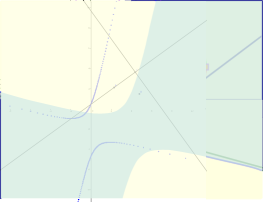
Figure 8.1: A ball and three lines. Each line induces a halfspace which lies below the line. In the dual, this corresponds to three vertically upward rays.

Summarizing the above discussion, the problem of computing the Tukey ball is equivalent to the following.

Problem 8.3.

Let $P\subset\mathbb{R}^{d}$ be a set of $n$ points in general position. The goal is to compute the ball $\mathsf{b}$, of smallest radius, such that (recalling Definition 2.3):

1. each point of the top $k$-level $T_{k}(P^{\star})$, the vertical upward ray intersects $\mathsf{b}^{\star}$, and

2. each point of the bottom $k$-level $B_{k}(P^{\star})$, the vertical downward ray intersects $\mathsf{b}^{\star}$.

Lemma 8.4.

Let $P\subset\mathbb{R}^{d}$ be a set of $n$ points in general position and $k\leq n$ a parameter. The Tukey ball can be computed in $O(n^{d-1}\log n)$ expected time.

Proof:

The proof uses Theorem 4.5 to solve the dual problem (this problem is LP-type with constant combinatorial dimension, where the constant depends on $d$). The input consists of a simplex $\Delta$, the set of hyperplanes $H=P^{\star}\cap\Delta$ intersecting $\Delta$, and the number of hyperplanes lying above and below $\Delta$. A given input can be decomposed using cuttings, as in the algorithms for Theorem 6.9, and Theorem 7.5.

We sketch the decision procedure. Given a candidate ball $\mathsf{b}$, we want to decide if $\mathsf{b}^{\star}$ violates any constraints induced by $H$. Equivalently, $\mathsf{b}^{\star}$ is an invalid solution if either condition holds: (i) there is a element of $T_{k}(P^{\star})$ which is above the top branch of $\mathsf{b}^{\star}$, or (ii) there is a element of $B_{k}(P^{\star})$ which is below the bottom branch of $\mathsf{b}^{\star}$. As such, a straightforward modification of the decision procedure described in Lemma 6.6 yields a decider in $O(\left|{H}\right|^{d-1}\log\left|{H}\right|)$ expected time.  

8.1.1 Improved algorithm

Lemma 8.5.

Let $P\subset\mathbb{R}^{d}$ be a set of $n$ points in general position and $k\leq n$ a parameter. The Tukey ball can be computed in $\scalerel*{\widetilde{O}}{j^{2}}\left({k^{d-1}\big{(}1+(n/k)^{\left\lfloor{d/2}\right\rfloor}\big{)}}\right)$ expected time.

Proof:

The algorithm is the same as described in Lemma 6.13 with a small change: compute a shallow cutting for the top $(\leq k)$-level and bottom $(\leq k)$-level of $P^{\star}$. Now run the randomized incremental algorithm of Lemma 6.13 on these collection of simplices with Lemma 8.4 as a black box to solve the subproblems of smaller size.  

8.2 The center ball in the dual

For a parameter $k$, recall that our goal is to compute the largest ball which lies inside all open halfspaces containing more than $n-k$ points of $P$. From the discussion above, in the dual this corresponds to the following problem.

Problem 8.6.

Let $P\subset\mathbb{R}^{d}$ be a set of $n$ points in general position. The goal is to compute the ball $\mathsf{b}$ of largest radius such that:

1. each point of the top $k$-level $T_{k}(P^{\star})$ lies below the bottom branch of $\mathsf{b}^{\star}$, and

2. each point of the bottom $k$-level $B_{k}(P^{\star})$ lies above the top branch of $\mathsf{b}^{\star}$.

Lemma 8.7.

Let $P\subset\mathbb{R}^{d}$ be a set of $n$ points in general position and $k\leq n$ a parameter. The center ball can be computed in $O(n^{d-1}\log n)$ expected time.

Proof:

As usual, we use Theorem 4.5 to solve the dual problem (this problem is LP-type with constant combinatorial dimension, where the constant depends on $d$). The input consists of a simplex $\Delta$, the set of hyperplanes $H=P^{\star}\cap\Delta$ intersecting $\Delta$, and the number of hyperplanes lying above and below $\Delta$. A given input can be decomposed using cuttings, as used in previous algorithms.

We sketch the decision procedure. We are also given a candidate ball $\mathsf{b}$. The algorithm computes the zone $\mathcal{Z}\left({\partial\Delta,H}\right)$ and computes the level of each vertex of $\mathcal{Z}\left({\partial\Delta,H}\right)$ inside $\Delta$ (taking into account the number of hyperplanes above and below $\Delta$). If we find a vertex of either the top or bottom $k$-level which also lies inside $\mathsf{b}^{\star}$, we report the violated constraint. Otherwise, if we find a vertex of the top $k$-level lying above the top branch of $\mathsf{b}^{\star}$ or a vertex of the bottom $k$-level lying below the bottom branch of $\mathsf{b}^{\star}$, then the solution $\mathsf{b}$ is also deemed infeasible. This decision procedure can be implemented in $O(\left|{H}\right|^{d-1}\log\left|{H}\right|)$ expected time.  

8.2.1 Improved algorithm

Lemma 8.8.

Let $P\subset\mathbb{R}^{d}$ be a set of $n$ points in general position and $k\leq n$ a parameter. The center ball can be computed in $\scalerel*{\widetilde{O}}{j^{2}}\left({k^{d-1}\big{(}1+(n/k)^{\left\lfloor{d/2}\right\rfloor}\big{)}}\right)$ expected time.

Proof:

The same argument for Lemma 8.5 applies here, using Lemma 8.7 as a black box to solve the subproblems generated by the $k$-shallow cutting of the top $(\leq k)$-level and bottom $(\leq k)$-level.  

9 Smallest disk of all vertices within crossing distance $k$

Let $L$ be a set of lines in the plane. For two points $p,{z}\in\mathbb{R}^{2}$, the crossing distance $\mathsf{d}_{L}(p,{z})$ is the number of lines of $L$ intersecting the segment $p{z}$.

Given a point ${z}\in\mathbb{R}^{2}$ not lying on any line of $L$, and a parameter $k$, let

$$S_{k}({z})=\left\{p\in\mathsf{V}\left({\mathcal{A}\left({L}\right)}\right)\;\middle|\;\mathsf{d}_{L}(p,{z})\leq k\right\}$$

be the set of vertices of $\mathcal{A}\left({L}\right)$ with crossing distance at most $k$ from ${z}$. The goal is to compute the smallest disk enclosing all points of $S_{k}({z})$, as shown in Figure 9.1.

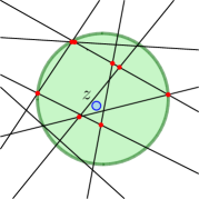
Figure 9.1: A disk containing all vertices of $\mathcal{A}\left({L}\right)$ lying within crossing distance at most three from ${z}$.

Lemma 9.1.

Let $L$ be a set of $n$ lines in the plane and let ${z}\in\mathbb{R}^{2}$ be a point not lying on any point of $L$. In $O(n\log n)$ expected time, one can compute the smallest disk enclosing all vertices of $\mathcal{A}\left({L}\right)$ within crossing distance at most $k$ from ${z}$.

Proof:

When the constraints (points) are explicitly given, this problem is LP-type with constant combinatorial dimension. We now apply Theorem 4.5 to obtain an efficient algorithm for this problem:

1. Each subproblem consists of a simplex $\Delta$, the set of lines $L^{\prime}=L\cap\Delta$, and a number $\mathsf{u}$ which is the number of lines of $L$ separating $\Delta$ and ${z}$. Given a disk $\mathsf{o}$ defined by the basis, check if there is a vertex of $\mathcal{A}\left({L^{\prime}}\right)$ which lies outside $\mathsf{o}$ and has crossing distance at most $k$ from ${z}$.

   To this end, compute the zone $\mathcal{Z}\left({\partial\Delta,L^{\prime}}\right)$. The algorithm chooses a vertex $v$ of $\mathcal{Z}\left({\partial\Delta,L^{\prime}}\right)$ inside $\Delta$ and computes $\mathsf{d}_{L}(v,{z})=\mathsf{d}_{L^{\prime}}(v,{z})+\mathsf{u}$. Next, walk around the set of vertices in $\mathcal{Z}\left({\partial\Delta,L^{\prime}}\right)\cap\Delta$ and compute the crossing values using previously computed crossing values. If at any time a vertex of crossing value at most $k$ which is outside $\mathsf{o}$ is encountered, report that $\mathsf{o}$ is an invalid solution.

2. The subproblem $(\Delta,L^{\prime},\mathsf{u})$ can be decomposed once again using cuttings. Compute a $(1/c)$-cutting (for sufficiently large constant $c$) of $L^{\prime}$ and clip the cutting inside $\Delta$. For each cell $\Delta_{i}$ in the cutting, compute $L^{\prime}\cap\Delta_{i}$ and the number of lines separating $\Delta_{i}$ from ${z}$.

The running time of the algorithm is dominated by the running time of the violation test, which is proportional to the complexity of the zone $\mathcal{Z}\left({\partial\Delta,L^{\prime}}\right)$. By Lemma 2.5, the violation test runs in $\mathcal{D}\left({n}\right)=O(n\log n)$ time.  

10 Conclusions

Since the conference version of [Cha04], several applications of the implicit LP technique have been found. For example, see [ACSS06, BM19, EW07, Mor08].

The natural open problem is to improve the running times for computing the yolk (and extremal yolk) even further. It seems believable, that for $d>3$, the log factor in Theorem 6.9 might not be necessary. We leave this as an open problem for further research.

Acknowledgments

The first author thanks Stefan Langerman for re-posing the problem of computing the maximum Tukey depth of a point set at the 2002 Fall Workshop on Computational Geometry problem session, and for subsequent discussions.

The authors thank Joachim Gudmundsson for bringing the problem of computing the yolk to our attention. The last author thanks Sampson Wong for discussions on computing the yolk in higher dimensions.

Finally, the authors thank the anonymous referees for the detailed comments and review.

Appendix A Proof sketch of Lemma 6.12

Let $H$ be set of $n$ hyperplanes in $\mathbb{R}^{d}$. We focus on constructing a $k$-shallow cutting when $d\geq 4$ (for $d<4$, we can construct shallow cuttings in $O(n\log n)$ deterministic time [CT16]). The original proof of existence of $k$-shallow cuttings by Matoušek [Mat92] provides a randomized algorithm for constructing such a cutting.

At a high level, the approach of Matoušek for constructing a $k$-shallow cutting is the following:

1. Let $R\subseteq H$ be a random sample of size $n/k$ and compute a bottom-vertex triangulation of $\mathcal{A}\left({R}\right)$. Let $\Xi$ denote the resulting set of simplices.

2. Let $\Xi^{\prime}\subseteq\Xi$ be the subset of simplices containing a point of level at most $k$ (with respect to $H$).

3. For each $\Delta\in\Xi^{\prime}$, if $\Delta$ intersects $tk$ hyperplanes of $H$ for some $t>1$, compute a $(1/t)$-cutting of the hyperplanes intersecting $\Delta$ and clip the cutting inside $\Delta$. Return this 2-level cutting as the desired $k$-shallow cutting.

A.1 Computing the top-level cutting

The top-level cutting is computed via randomized incremental construction. The algorithm randomly permutes the hyperplanes of $H$, label them $h_{1},\ldots,h_{n}$ and let $H_{i}=\{h_{1},\ldots,h_{i}\}$. For $i=1,\ldots,n/k$, the algorithm maintains a collection of simplices, formed from the arrangement $\mathcal{A}\left({H_{i}}\right)$ and which contain a point of level $k$ (with respect to $H$). Each simplex $\Delta$ maintains pointers to the subset of hyperplanes $\{h_{i+1},\ldots,h_{n}\}$ which intersect $\Delta$ (this is the conflict list of $\Delta$). Each hyperplane $h_{j}$ for $j>i$ also maintains reverse pointers to the set of simplices it intersects in the current triangulation. Finally, each cell in the arrangement maintains the number of hyperplanes of $H$ which lie strictly below it.

In an update step, insert the hyperplane $h_{i}$. Using the reverse pointers, we determine the set of simplices that are split by inserting $h_{i}$ into the current arrangement. Using these simplices, we can find the cells that are split by $h_{i}$. Fix a cell $C$ intersected by $h_{i}$ and let $H_{C}\subseteq H\setminus H_{i}$ be the union of the conflict lists over the simplices in $C$. Suppose $C$ is split into two new cells $C_{1}$ and $C_{2}$. Assume $C_{1}$ lies above $h_{i}$. We determine the number of planes lying below $C_{1}$ ($C_{2}$ can be handled symmetrically). Let $v$ be a vertex of $C$ lying below $h_{i}$. From $v$, we perform a graph search on the boundary of $C$ to determine the number of hyperplanes of $H_{C}$ lying strictly below $C_{1}$ (adding the number of hyperplanes lying below $C$ to the count). If at any point this count is greater than $k$, we discard $C_{1}$, as it does not cover the $(\leq k)$-level. This process is repeated for all cells split by $h_{i}$. At the end of the process, we triangulate the newly created cells, and construct the conflict lists for the new simplices. See [BDS95, Section 5.4] for details on how to efficiently maintain the conflict lists and arrangement incrementally.

A.2 Refining the cutting

At the end of the process, the algorithm has a collection of simplices $\Xi$ which cover the $(\leq k)$-level. For each simplex $\Delta\in\Xi$, if $\Delta$ has conflict list size $tk$ for some $t\geq 1$, compute a $(1/t)$-cutting for the hyperplanes intersecting $\Delta$ and clip the cutting inside $\Delta$. This ensures that every simplex in the final two-level cutting intersects at most $k$ hyperplanes of $H$.

A.3 Analysis sketch

In each step of the randomized incremental algorithm, the total amount of work done is proportional to the size of the conflict lists destroyed or created. Let $\Xi_{i}$ denote the current collection of simplices at step $i$, where $\Xi=\Xi_{n/k}$ is the collection of cells in the top-level cutting at the end of the process. We first analyze the total size of the conflict lists over all simplices in $\Xi_{i}$. For each $\Delta\in\Xi_{i}$, let $w(\Delta)$ be the size of the conflict list of $\Delta$. For an integer $t\geq 1$, let $\Xi_{i}[t]=\left\{\Delta\in\Xi_{i}\;\middle|\;(t-1)k<w(\Delta)\leq tk\right\}$. In the original proof of the shallow cutting lemma Matoušek proved that, roughly speaking, the number of simplices in $\Xi_{i}$ with $w(\Delta)\in((t-1)k,tk]$ is decays exponentially in $t$—formally $\mathop{\mathbf{E}}\!\left[{\left|{\Xi_{i}[t]}\right|}\right]=O(2^{-t}\left|{\Xi_{i}}\right|)$ [Mat92, Lemma 2.4]. Using this, one can bound the sum of the conflict list sizes as (see [BDS95, Theorem 3] and [Har11, Theorem 8.8]):

$$\alpha_{i}:=\mathop{\mathbf{E}}\!\left[{\sum_{\Delta\in\Xi_{i}}w(\Delta)}\right]=O\left({\left|{\Xi_{i}}\right|(n/i)}\right)=O\left({i^{\left\lfloor{d/2}\right\rfloor}(n/i)}\right).$$

Since the hyperplanes were randomly permuted, we have that that the amortized work done in the $i$th step of the algorithm is $O(\alpha_{i}/i)$ [BDS95, Theorem 5]. As such, the expected running time to compute the top-level cutting is bounded by:

$$\sum_{i=1}^{n/k}O\left({\frac{\alpha_{i}}{i}}\right)=O\left({\sum_{i=1}^{n/k}\frac{ni^{\left\lfloor{d/2}\right\rfloor}}{i^{2}}}\right)=O\left({\frac{n}{k}\cdot n\left({\frac{n}{k}}\right)^{\left\lfloor{d/2}\right\rfloor-2}}\right)=O\left({k\left({\frac{n}{k}}\right)^{\left\lfloor{d/2}\right\rfloor}}\right),$$

where in the second inequality we use the assumption $d\geq 4$. (For $d<4$, the summation solves to $O(n\log(n/k))$.)

As for the second level cutting, fix a simplex $\Delta\in\Xi[t]$ with weight $w(\Delta)\in((t-1)k,tk]$. Computing a $(1/t)$-cutting inside $\Delta$ costs $O(w(\Delta)t^{d-1})=O(t^{d}k)$ expected time [Cha93]. Thus, the expected running time of the second-level cutting is bounded by $O\left({k\sum_{t=1}^{\infty}\sum_{\Delta\in\Xi[t]}t^{d}}\right)$. Again, by the properties of exponential decay [Mat92, BDS95, Har11] we have that

$$\mathop{\mathbf{E}}\!\left[{k\sum_{t\geq 1}\sum_{\Delta\in\Xi[t]}t^{d}}\right]=O\left({k\left({n/k}\right)^{\left\lfloor{d/2}\right\rfloor}}\right).$$

This completes the proof of Lemma 6.12.

References

- [ACG+02] Greg Aloupis et al. “Lower bounds for computing statistical depth” In Computational Statistics & Data Analysis 40.2 Elsevier, 2002, pp. 223–229 DOI: 10.1016/S0167-9473(02)00032-4
- [ACSS06] Pankaj K. Agarwal, Sergio Cabello, Joan Antoni Sellarès and Micha Sharir “Computing a Center-Transversal Line” In Proc. 26th International Conference on Foundations of Software Technology and Theoretical Computer Science (FSTTCS), 2006, pp. 93–104 DOI: 10.1007/11944836\_11
- [ALST03] Greg Aloupis, Stefan Langerman, Michael A. Soss and Godfried T. Toussaint “Algorithms for bivariate medians and a Fermat-Torricelli problem for lines” In Comput. Geom. Theory Appl. 26.1, 2003, pp. 69–79 DOI: 10.1016/S0925-7721(02)00173-6
- [APS93] Boris Aronov, Marco Pellegrini and Micha Sharir “On the Zone of a Surface in a Hyperplane Arrangement” In Discrete Comp. Geom. 9, 1993, pp. 177–186 DOI: 10.1007/BF02189317
- [AS98] P.. Agarwal and M. Sharir “Efficient algorithms for geometric optimization” In ACM Comput. Surv. 30.4, 1998, pp. 412–458 DOI: 10.1145/299917.299918
- [ASW08] Pankaj K. Agarwal, Micha Sharir and Emo Welzl “Algorithms for center and Tverberg points” In ACM Trans. Algorithms 5.1, 2008, pp. 5:1–5:20 DOI: 10.1145/1435375.1435380
- [BCG19] Mark Berg, Jonathan Chung and Joachim Gudmundsson “Computing the Yolk in Spatial Voting Games” unpublished manuscript, 2019
- [BCKO08] M. Berg, O. Cheong, M. van Kreveld and M.. Overmars “Computational Geometry: Algorithms and Applications” Santa Clara, CA, USA: Springer-Verlag, 2008 DOI: 10.1007/978-3-540-77974-2
- [BDS95] Mark Berg, Katrin Dobrindt and Otfried Schwarzkopf “On Lazy Randomized Incremental Construction” In Discrete Comp. Geom. 14.3, 1995, pp. 261–286 DOI: 10.1007/BF02570705
- [BE02] Marshall W. Bern and David Eppstein “Multivariate Regression Depth” In Discrete Comp. Geom. 28.1, 2002, pp. 1–17 DOI: 10.1007/s00454-001-0092-1
- [BGM18] Mark Berg, Joachim Gudmundsson and Mehran Mehr “Faster Algorithms for Computing Plurality Points” In ACM Trans. Algorithms 14.3, 2018, pp. 36:1–36:23 DOI: 10.1145/3186990
- [BJMR94] Binay K. Bhattacharya, Shreesh Jadhav, Asish Mukhopadhyay and Jean-Marc Robert “Optimal algorithms for some intersection radius problems” In Computing 52.3, 1994, pp. 269–279 DOI: 10.1007/BF02246508
- [Bla48] Duncan Black “On the Rationale of Group Decision-making” In Journal of Political Economy 56.1, 1948, pp. 23–34 DOI: 10.1086/256633
- [BM19] Luis Barba and Wolfgang Mulzer “Asymmetric Convex Intersection Testing” In Proc. 2nd Symposium on Simplicity in Algorithms (SOSA), 2019, pp. 9:1–9:14 DOI: 10.4230/OASIcs.SOSA.2019.9
- [CEM+96] Kenneth L. Clarkson et al. “Approximating center points with iterative Radon points” In Internat. J. Comput. Geom. Appl. 6, 1996, pp. 357–377 DOI: 10.1142/S021819599600023X
- [Cha04] Timothy M. Chan “An optimal randomized algorithm for maximum Tukey depth” In Proc. 15th ACM-SIAM Sympos. Discrete Algs. (SODA) SIAM, 2004, pp. 430–436 URL: http://dl.acm.org/citation.cfm?id=982792.982853
- [Cha93] Bernard Chazelle “Cutting Hyperplanes for Divide-and-Conquer” In Discrete Comp. Geom. 9, 1993, pp. 145–158 DOI: 10.1007/BF02189314
- [Cha96] Timothy M. Chan “Fixed-Dimensional Linear Programming Queries Made Easy” In Proc. 12th Annu. Sympos. Comput. Geom. (SoCG) ACM, 1996, pp. 284–290 DOI: 10.1145/237218.237397
- [Cha99] Timothy M. Chan “Geometric Applications of a Randomized Optimization Technique” In Discrete Comp. Geom. 22.4, 1999, pp. 547–567 DOI: 10.1007/PL00009478
- [Cha99a] Timothy M. Chan “Remarks on -level algorithms in the plane” In Manuscript, 1999
- [Cla95] Kenneth L. Clarkson “Las Vegas Algorithms for Linear and Integer Programming when the Dimension is Small” In J. ACM 42.2, 1995, pp. 488–499 DOI: 10.1145/201019.201036
- [Cla97] Kenneth L. Clarkson “Algorithms for the minimum diameter of moving points and for the discrete 1-center problem” In Manuscript, 1997 URL: http://cm.bell-labs.com/who/clarkson/moving%5C_diam.html
- [CLRS01] Thomas H. Cormen, Charles E. Leiserson, Ronald L. Rivest and Clifford Stein “Introduction to Algorithms” McGraw-Hill, 2001
- [Col87] Richard Cole “Slowing down sorting networks to obtain faster sorting algorithms” In J. Assoc. Comput. Mach. 34.1, 1987, pp. 200–208 DOI: 10.1145/7531.7537
- [CS89] K.. Clarkson and P.. Shor “Applications of random sampling in computational geometry, II” In Discrete Comp. Geom. 4, 1989, pp. 387–421 DOI: 10.1007/BF02187740
- [CSY87] Richard Cole, Micha Sharir and Chee-Keng Yap “On -Hulls and Related Problems” In SIAM J. Comput. 16.1, 1987, pp. 61–77 DOI: 10.1137/0216005
- [CT16] Timothy M. Chan and Konstantinos Tsakalidis “Optimal Deterministic Algorithms for 2-d and 3-d Shallow Cuttings” In Discrete Comp. Geom. 56.4, 2016, pp. 866–881 DOI: 10.1007/s00454-016-9784-4
- [Dey98] Tamal K Dey “Improved bounds for planar -sets and related problems” In Discrete Comp. Geom. 19.3 Springer, 1998, pp. 373–382 DOI: 10.1007/PL00009354
- [Epp03] David Eppstein “Setting Parameters by Example” In SIAM J. Comput. 32.3, 2003, pp. 643–653 DOI: 10.1137/S0097539700370084
- [Eri99] Jeff Erickson “New Lower Bounds for Convex Hull Problems in Odd Dimensions” In SIAM J. Comput. 28.4, 1999, pp. 1198–1214 DOI: 10.1137/S0097539797315410
- [ESS93] Herbert Edelsbrunner, Raimund Seidel and Micha Sharir “On the Zone Theorem for Hyperplane Arrangements” In SIAM J. Comput. 22.2, 1993, pp. 418–429 DOI: 10.1137/0222031
- [EW07] David Eppstein and Kevin A. Wortman “Minimum dilation stars” In Comput. Geom. 37.1, 2007, pp. 27–37 DOI: 10.1016/j.comgeo.2006.05.007
- [GJS96] Prosenjit Gupta, Ravi Janardan and Michiel H.. Smid “Fast Algorithms for Collision and Proximity Problems Involving Moving Geometric Objects” In Comput. Geom. Theory Appl. 6, 1996, pp. 371–391 DOI: 10.1016/0925-7721(95)00028-3
- [GSW92] Joseph Gil, William L. Steiger and Avi Wigderson “Geometric medians” In Discret. Math. 108.1-3, 1992, pp. 37–51 DOI: 10.1016/0012-365X(92)90658-3
- [GW19] Joachim Gudmundsson and Sampson Wong “Computing the Yolk in Spatial Voting Games without Computing Median Lines” In 33th Conf. Artificial Intell. (AAAI), 2019, pp. 2012–2019
- [GW19a] Joachim Gudmundsson and Sampson Wong “Computing the Yolk in Spatial Voting Games without Computing Median Lines” In CoRR abs/1902.04735, 2019 arXiv: http://arxiv.org/abs/1902.04735
- [Har11] S. Har-Peled “Geometric Approximation Algorithms” 173, Math. Surveys & Monographs Boston, MA, USA: Amer. Math. Soc., 2011 DOI: 10.1090/surv/173
- [Har16] Sariel Har-Peled “Shortest path in a polygon using sublinear space” In J. Comput. Geom. 7.2, 2016, pp. 19–45 DOI: 10.4230/LIPIcs.SOCG.2015.111
- [HJ19] Sariel Har-Peled and Mitchell Jones “Journey to the Center of the Point Set” In Proc. 35th Int. Annu. Sympos. Comput. Geom. (SoCG) 129, 2019, pp. 41:1–41:14 DOI: 10.4230/LIPIcs.SoCG.2019.41
- [HJ20] Sariel Har-Peled and Mitchell Jones “Fast Algorithms for Geometric Consensuses” In Proc. 36th Int. Annu. Sympos. Comput. Geom. (SoCG) 164, LIPIcs Schloss Dagstuhl - Leibniz-Zentrum für Informatik, 2020, pp. 50:1–50:16 DOI: 10.4230/LIPIcs.SoCG.2020.50
- [JM94] Shreesh Jadhav and Asish Mukhopadhyay “Computing a Centerpoint of a Finite Planar Set of Points in Linear Time” In Discrete Comp. Geom. 12, 1994, pp. 291–312 DOI: 10.1007/BF02574382
- [Kal92] G. Kalai “A subexponential randomized simplex algorithm” In Proc. 24th Annu. ACM Sympos. Theory Comput. (STOC), 1992, pp. 475–482
- [Kin97] Valerie King “A Simpler Minimum Spanning Tree Verification Algorithm” In Algorithmica 18.2, 1997, pp. 263–270 DOI: 10.1007/BF02526037
- [KKT95] David R. Karger, Philip N. Klein and Robert Endre Tarjan “A Randomized Linear-Time Algorithm to Find Minimum Spanning Trees” In J. ACM 42.2, 1995, pp. 321–328 DOI: 10.1145/201019.201022
- [KMR+08] Marc J. Kreveld et al. “Efficient Algorithms for Maximum Regression Depth” In Discrete Comp. Geom. 39.4, 2008, pp. 656–677 DOI: 10.1007/s00454-007-9046-6
- [LS00] Stefan Langerman and William Steiger “Computing a maximal depth point in the plane” In Proc. Japan Conf. Discrete Comput. Geom. (JCDCG), 2000
- [LS03] Stefan Langerman and William Steiger “The complexity of hyperplane depth in the plane” In Discrete Comp. Geom. 30.2 Springer, 2003, pp. 299–309 DOI: 10.1007/s00454-003-0011-x
- [LS03a] Stefan Langerman and William L. Steiger “Optimization in Arrangements” In Proc. 20th Sympos. Theoret. Aspects Comput. Sci. (STACS) 2607, Lecture Notes in Computer Science Springer, 2003, pp. 50–61 DOI: 10.1007/3-540-36494-3\_6
- [Mat02] Jiří Matoušek “Lectures on Discrete Geometry” 212, Grad. Text in Math. Springer, 2002 DOI: 10.1007/978-1-4613-0039-7/
- [Mat90] Jiří Matoušek “Computing the Center of Planar Point Sets” In Discrete Comp. Geom.: Papers from the DIMACS Special Year 6, DIMACS Series in Discrete Mathematics and Theoretical Computer Science DIMACS/AMS, 1990, pp. 221–230 DOI: 10.1090/dimacs/006/14
- [Mat92] Jiří Matoušek “Reporting Points in Halfspaces” In Comput. Geom. 2, 1992, pp. 169–186 DOI: 10.1016/0925-7721(92)90006-E
- [Mat93] Jiří Matoušek “Linear Optimization Queries” In J. Algorithms 14.3, 1993, pp. 432–448 DOI: 10.1006/jagm.1993.1023
- [McK86] Richard D. McKelvey “Covering, Dominance, and Institution-Free Properties of Social Choice” In American Journal of Political Science 30.2, 1986, pp. 283–314 DOI: 10.2307/2111098
- [Meg83] Nimrod Megiddo “Applying Parallel Computation Algorithms in the Design of Serial Algorithms” In J. Assoc. Comput. Mach. 30.4, 1983, pp. 852–865 DOI: 10.1145/2157.322410
- [Meg84] N. Megiddo “Linear programming in linear time when the dimension is fixed” In J. Assoc. Comput. Mach. 31, 1984, pp. 114–127 DOI: 10.1145/2422.322418
- [Mor08] Pat Morin “An optimal randomized algorithm for -variate zonoid depth” In Comput. Geom. 39.3, 2008, pp. 229–235 DOI: 10.1016/j.comgeo.2006.12.002
- [MRR+03] Kim Miller et al. “Efficient computation of location depth contours by methods of computational geometry” In Stat. Comput. 13.2, 2003, pp. 153–162 DOI: 10.1023/A:1023208625954
- [MSW96] J. Matoušek, M. Sharir and E. Welzl “A Subexponential Bound for Linear Programming” In Algorithmica 16.4/5, 1996, pp. 498–516 DOI: 10.1007/BF01940877
- [NS90] Nir Naor and Micha Sharir “Computing a point in the center of a point set in three dimensions” In Proc. 2nd Canad. Conf. Comput. Geom. (CCCG), 1990, pp. 10–13
- [OA19] Eunjin Oh and Hee-Kap Ahn “Computing the center region and its variants” In Theor. Comput. Sci. 789, 2019, pp. 2–12 DOI: 10.1016/j.tcs.2018.06.026
- [OV04] R. Oostrum and R.. Veltkamp “Parametric search made practical” In Comput. Geom. Theory Appl. 28.2-3, 2004, pp. 75–88
- [Ram00] Edgar A. Ramos “Linear programming queries revisited” In Proc. 16th Annu. Sympos. Comput. Geom. (SoCG) ACM, 2000, pp. 176–181 DOI: 10.1145/336154.336198
- [Ram01] Edgar A. Ramos “An Optimal Deterministic Algorithm for Computing the Diameter of a Three-Dimensional Point Set” In Discret. Comput. Geom. 26.2, 2001, pp. 233–244 DOI: 10.1007/s00454-001-0029-8
- [RR96] Ida Ruts and Peter J Rousseeuw “Computing depth contours of bivariate point clouds” In Computational Statistics & Data Analysis 23.1 Elsevier, 1996, pp. 153–168 DOI: 10.1016/S0167-9473(96)00027-8
- [RR98] Peter J Rousseeuw and Ida Ruts “Constructing the bivariate Tukey median” In Statistica Sinica 8 JSTOR, 1998, pp. 827–839 URL: https://www.jstor.org/stable/24306466
- [Rub79] Ariel Rubinstein “A Note about the “Nowhere Denseness” of Societies Having an Equilibrium under Majority Rule” In Econometrica 47.2, 1979, pp. 511–514 DOI: 10.2307/1914198
- [Sei91] Raimund Seidel “Small-Dimensional Linear Programming and Convex Hulls Made Easy” In Discrete Comp. Geom. 6, 1991, pp. 423–434 DOI: 10.1007/BF02574699
- [Sma90] Christopher G. Small “A survey of multidimensional medians” In Internat. Statist. Rev 58 JSTOR, 1990, pp. 263–277 DOI: 10.2307/1403809
- [ST92] Richard E. Stone and Craig A. Tovey “Limiting median lines do not suffice to determine the yolk” In Social Choice and Welfare 9.1 Springer, 1992, pp. 33–35 DOI: 10.1007/BF00177668
- [SW92] Micha Sharir and Emo Welzl “A Combinatorial Bound for Linear Programming and Related Problems” In Proc. 9th Sympos. on Theoretical Aspects of Comput. Sci. (STACS), 1992, pp. 569–579 DOI: 10.1007/3-540-55210-3_213
- [Tót01] Géza Tóth “Point Sets with Many k-Sets” In Discrete Comp. Geom. 26.2, 2001, pp. 187–194 DOI: 10.1007/s004540010022
- [Tov92] Craig A. Tovey “A polynomial-time algorithm for computing the yolk in fixed dimension” In Math. Program. 57, 1992, pp. 259–277 DOI: 10.1007/BF01581084
- [Tuk75] John W. Tukey “Mathematics and the picturing of data” In Proc. Int. Congress of Mathematicians 2, 1975, pp. 523–531 DOI: 10.1090/S0002-9939-96-03657-X