Precision of mass and radius determination for neutron star using the ATHENA mission.

Abstract

In this paper we show that X-ray spectral observations of the ATHENA mission, which is planned to launch in 2031, can constrain the equation of state of superdense matter. We use our well-constrained continuum fitting method for mass and radius determination of the neutron star. Model spectra of the emission from a neutron star were calculated using the atmosphere code ATM24. In the next step, those models were fitted to a simulated spectra of the neutron star calculated for ATHENA’s WFI detector, using the satellite calibration files. To simulate the spectra we assumed three different values of effective temperatures, surface gravities and gravitational redshifts. There cases are related to the three different neutron star masses and radii. This analysis allows us to demonstrate the precision of our method and demonstrate the need for a fast detector onboard of ATHENA. A large grid of theoretical spectra was calculated with various parameters and a hydrogen-helium-iron composition of solar proportion. These spectra were fitted to the simulated spectrum to estimate the precision of mass and radius determination. In each case, we obtained very precise mass and radius values with errors in the range 3–10% for mass and in the range 2–8% for radius within the $1\sigma$ confidence error. We show here that with the ATHENA WFI detector, such a determination could be used to constrain the equation of state of superdense neutron star matter.

1 INTRODUCTION

Almost 50 years after confirmation of the existence of the neutron star (Hewish et al., 1968), the equation of state of the matter that comprises these stars is still under discussion. In neutron stars, the density in the center of the star exceeds a few times the nuclear density. Many theoretical models of the equation of state (EOS) of superdense matter have been proposed, (see the extensive review by Haensel et al., 2007). Models have assumed both normal matter and matter in exotic states, like condensates of pions or kaons, superfluid or superconductive matter, or even free quarks. Astronomical observations are the only way to verify the EOS of neutron stars, because in Earth laboratories we are unable to reproduce conditions similar to neutron star interiors. A very important property of theoretical models is the existence of a maximum mass for the neutron star and a unique mass – radius relation for each assumed EOS. There exist multiple methods to constrain the EOS with astronomical observations.

Astronomers seek to uncover the heaviest neutron stars (Antoniadis et al., 2013; Demorest et al., 2010). Measurements of the maximum mass allows one to exclude those EOS models that predict a maximum mass lower than the observed maximum. Comparison of both masses does not allow one for the unique determination of the EOS. There exist methods that allow for simultaneous mass and radius determination, and consequently, to determine the EOS. One such method is fitting of the observed spectra with model atmospheres, but until the necessary high-quality spectra are obtained, the accuracy of mass and radius determination will remain an open question. We expect that such high quality spectra can be obtained by the ATHENA detectors, especially that a growing population of bursters, currently numbered at 110 has been observed by almost every major X-ray satellite (Watts et al., 2016; Galloway & Keek, 2017, and references therein).

ATHENA (Advanced Telescope for High Energy Astrophysics) is an X-ray mission accepted by the ESA to address the Hot and Energetic Universe science theme (Nandra et al., 2013). The mission will be launched in 2031 and placed at the second Sun-Earth Lagrangian point (L2). The planned mission lifetime is five years, but the mission is expected to last longer. ATHENA will be equipped with two scientific instruments: the X-ray Integral Field Unit (X-IFU; Barret et al., 2013) and the Wide Field Imager (WFI; Rau et al., 2013).

As per its name, the WFI has a large field of view 40’$\times$40’, and very high angular resolution, 5”. It will observe in the energy range 0.2 – 15 keV with resolution 170 eV at 7 keV. The planned time resolution for this instrument is 80 $\mu$sec. It’s scientific goals are related to high energy phenomena, and include studying hot baryons in groups and clusters of galaxies, accretion processes onto compact objects, and GRBs and other transient objects. The high time resolution of WFI in combination with the large effective area of the ATHENA mirrors make this detector fast enough to be used for studying neutron stars during bursts. Such conditions are needed for mass and radius determination when using the continuum fitting method.

The continuum fitting method was first described by Majczyna & Madej (2005). They fit PCA/RXTE spectra of MXB 1728$-$34 taken during a phase between the bursts. Each spectrum was integrated over 16 s. These authors fit numerical models calculated with the ATM21 code to the observed spectra. Furthermore, the same models were fitted to the observed spectra of 4U 1820$-$30 (Kuśmierek et al., 2011). They obtained values of mass $M=1.3\pm 0.6\,$M_⊙ and radius $R=11^{+3}_{-2}\,$km consistent with results obtained by other researchers. Errors in the paper by Kuśmierek et al. (2011) are relatively large but they could be reduced if some systematic effects known now (e.g. accretion during even strong bursts) are included. Continuum fitting method for neutron star mass and radius determination can be also used without complicated calculations of neutron star atmospheres. Instead, black body emission multiplied by the color correction factor can be assumed (Özel et al., 2009). Such approach is faster, but it does not take into account that in reality, the overall shape of the emitted spectrum is modified by Compton scattering, especially at the hard tail of the spectrum (Majczyna & Madej, 2005; Suleimanov et al., 2011).

In our analysis we used fake spectra, therefore, we made the principal assumption that our theoretical models are valid for this “source”. Therefore, we did not widely discuss validation of each assumption of our model in context of real sources. But we will note that our theoretical spectra could be used to fit the observed spectra of real sources (see eg. Kuśmierek et al. (2011)). In this paper, we clearly show that the data which will be provided by WFI/ATHENA will allow us to determine mass and radius, using continuum fitting method, with errors as small as 3-10% for mass determination and 2-8% for radius determination even for relatively dim sources.

2 THE ATM24 MODEL CODE

The model atmospheres and theoretical X-ray spectra of hot neutron stars used in this paper were computed with the ATM24 code, which is the next version of ATM21 code (Madej, 1991; Majczyna et al., 2005) upgraded for its numerical precision. The accuracy of the code has been recently demonstrated by Madej et al. (2017); Vincent et al. (2018). The ATM24 code calculates the radiative transfer equation in a plane-parallel geometry. It takes into account the effect of Compton scattering on free, relativistic electrons, where initial photon energies can approach the electron rest mass. We assume the equation of state of ideal gas being in local thermodynamical equilibrium (LTE). Nevertheless, the Compton scattering redistribution functions of X-ray photons $\Phi(\nu,\nu^{\prime})$ are fully non-LTE terms of the radiative transfer equation.

The equation of transfer was adopted from Pomraning (1973, see also , ). The working equation of transfer and the temperature correction procedure were presented originally by Madej (1989, 1991) and used correctly by Madej et al. (2017); Vincent et al. (2018). The final equation of transfer is written on the monochromatic optical depth scale $d\tau_{\nu}=-(k_{\nu}+\sigma_{\nu})\,\rho\,dz$, and has a form:

$$\mu\,\frac{dI_{\nu}}{d\tau_{\nu}} = I_{\nu}-{\frac{k_{\nu}}{k_{\nu}+\sigma_{\nu}}}B_{\nu}-\left(1-{\frac{k_{\nu}}{k_{\nu}+\sigma_{\nu}}}\right)J_{\nu}+\left(1-{\frac{k_{\nu}}{k_{\nu}+\sigma_{\nu}}}\right)J_{\nu}\int\limits_{0}^{\infty}\Phi(\nu,\nu^{\prime})\left(1+{\frac{c^{2}}{2h{\nu^{\prime}}^{3}}}J_{\nu^{\prime}}\right)d\nu^{\prime}+$$ (1)

$$- {\frac{k_{\nu}}{k_{\nu}+\sigma_{\nu}}}\left(1+{\frac{c^{2}}{2h\nu^{3}}}J_{\nu}\right)\times\int\limits_{0}^{\infty}\Phi(\nu,\nu^{\prime})J_{\nu^{\prime}}{\left({\frac{\nu}{\nu^{\prime}}}\right)}^{3}\exp\left[-{\frac{h(\nu-\nu^{\prime})}{{\rm k}T}}\right]d\nu^{\prime},$$

where $k_{\nu}$ and $\sigma_{\nu}$ denote coefficients of absorption and electron scattering, respectively. $I_{\nu}$ is the energy-dependent specific intensity, $J_{\nu}$ is the mean intensity of radiation, and $z$ is the geometrical depth in the considered atmosphere.

We used the angle-averaged redistribution function $\Phi(\nu,\nu^{\prime})$ and Compton scattering cross-section $\sigma(\nu\to\nu^{\prime},\vec{n}\cdot\vec{n^{\prime}})$, following the method by Guilbert (1981), which was corrected for the computational error by Madej (1991). The Compton redistribution function is related to cross section as defined in Madej (1989):

$$\Phi(\nu,\nu^{\prime})={\frac{1}{\sigma_{\nu}}}\oint_{\omega^{\prime}}\frac{d\omega^{\prime}}{4\pi}\,\sigma(\nu\to\nu^{\prime},\vec{n}\cdot\vec{n^{\prime}}).$$ (2)

We solve the model atmosphere assuming constrains of hydrostatic and radiative equilibrium. We are aware that for atmosphere in motion this assumption is too strong, however, such models were widely used to fit the X-ray spectra (see e.g. Suleimanov et al. (2017); Medin et al. (2016)). The influences of the magnetic field and accretion onto the neutron star are not included. Our code takes into account energy-dependent opacities of hydrogen, helium and heavy element ions in LTE. The ionization equilibrium is fully solved, allowing for the appearance of iron lines for specific initial parameters Majczyna et al. (2005). We neglect the effects of electron degeneracy, which are unimportant in the hot atmospheres relevant to our studies. Examples of the theoretical local spectra for one value of effective temperature and several surface gravities are shown in the Figure 1. Near the maximum flux, a few emission iron lines are clearly seen.

Figure 1: Theoretical local spectrum of hot neutron star atmosphere with parameters: $T_{\rm eff}=2.20\times 10^{7}$ K and different surface gravities: left panel from $\log(g)=14.20$ to 14.60, whereas right one from 14.30 to 14.60. The assumed hydrogen-helium-iron composition if of solar proportion (left panel) and pure hydrogen atmosphere (right panel). On the right panel picture, we add to comparison spectrum of the atmosphere with iron and $\log(g)=14.40$ (solid, black line).

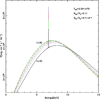
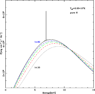
Right panel of Figure 1 shown spectra of hot neutron star calculated by ATM24 code for the same effective temperature $T_{\rm eff}=2.20\times 10^{7}\,$K and logarithm of surface gravity from $\log(g)=14.30$ up to $\log(g)=14.60$. We assumed pure hydrogen atmosphere. For comparison we also add spectrum of the atmosphere composed by mixture of hydrogen, helium and iron in following proportions: $N_{He}/N_{H}=0.11$ and $N_{Fe}/N_{H}=3.7\times 10^{-5}$ and $\log(g)=14.40$.

3 SIMULATED SPECTRUM

ATHENA is a future mission; therefore for the aim of this paper, we simulated a spectrum which will be detected by the WFI instrument. We used publicly available calibration files provided by the ATHENA mission team. The effective area at 1 keV is 1.4 m². To simulate the observed spectrum with WFI detector, we used “fake” command in xspec 12.6.0 fitting package (Arnaud, 1996). The above command works on theoretical model and simulates the data taking into account WFI/ATHENA responces and background files for the newest design of mirror with 15 rows¹. The obtained data file is accompanied by relevant simulated new background file. In the case of simulated spectrum and background all errors are Poissonian.

Table 1: Fake spectra parameters for A, B, and C model atmospheres: hydrogen column density $N_{H}$, effective temperature $T_{\rm eff}$, surface gravity $\log g$, gravitational redshift $z$ and normalization factor $N_{\rm ATM}$. In last three rows we display corresponding masses, radii and fluxes, $F$, for those sources.

name	A	B	C
$N_{H}$ [cm-2]	$0.8\times 10^{22}$	$0.8\times 10^{22}$	$0.8\times 10^{22}$
$T_{\rm eff}$ [K]	$2.19\times 10^{7}$	$2.20\times 10^{7}$	$2.21\times 10^{7}$
$\log g$ [cgs]	14.25	14.30	14.35
$z$	0.240	0.300	0.350
$N_{\rm ATM}$	2.5$\times 10^{-24}$	2.5$\times 10^{-24}$	2.5$\times 10^{-24}$
$M\,$[M⊙]	1.297	1.653	1.869
$R\,$[km]	10.956	11.954	12.230
$F$ [erg cm-2 s-1]	4.51 $\times 10^{-10}$	4.42 $\times 10^{-10}$	4.32 $\times 10^{-10}$

To produce simulated data, we chose three models with various parameters for the neutron star atmosphere: effective temperature $T_{\rm eff}$, surface gravity $\log g$, gravitational redshift $z$ and normalization factor $N_{\rm ATM}$ given in Table 1. We name those models as A, B, C respectively. The values of $\log g$ and $z$ correspond to particular masses and radii of a neutron stars also given in the above Table (see Section 5 for relation between parameters). The normalization factor is directly related with the ratio of the neutron star radius to the distance $D$ as $(R/D)^{2}$. We normalize our models in such a way, that the values of observed fluxes correspond to semi-bright Galactic X-ray sources. All observed fluxes are given in the last row of Table 1.

These parameters are not related to any particular existing neutron star, but compact objects with these parameters certainly could be realized in nature. The chemical composition was assumed as a mixture of hydrogen $N_{\rm He}/N_{\rm H}=0.11$ and iron $N_{\rm Fe}/N_{\rm H}=3.7\times 10^{-5}$ (number abundances). Corresponding relative mass abundances are: $M_{\rm H}$=0.6950, helium $M_{\rm He}$=0.3035 and iron $M_{\rm Fe}$=1.425$\times 10^{-3}$. Finally all our models were multiplied by interstellar absorption model (tbabs in xspec) with the same assumed hydrogen column density $N_{\rm H}=0.80\times 10^{22}\,$cm^-2. We set the time exposure $t_{\rm exp}$ equal to 1 second. Such a value of $t_{\rm exp}$ can be used for objects like isolated neutron stars or X-ray transients in the period when the neutron star is not accreting matter.

Figure 2: Simulated WFI spectra for arbitrarily chosen parameters: $T_{\rm eff}=2.2\times 10^{7}\,$K, $\log(g)=14.3$, $z=0.30$ and $N_{\rm ATM}=2.5\times 10^{-24}$ (fake spectrum B; black crosses) and $N_{\rm ATM}=2.5\times 10^{-25}$ (red). Systematic errors on the level of 3% are taken into account. The chemical composition is assumed as mixture of hydrogen, helium and iron in the solar proportion. The time exposure $t_{\rm exp}$ is equal to 1 second. The overall data are shaped by ATHENA mirrors and WFI effective area.

In the case of X-ray bursters, however, the situation is more complicated. In such objects the method based on fitting observed spectra should be used for photospheric radius expansion bursts in the touchdown phase in the hard state. In such a situation the exposure time should be much shorter of the order of tenths of a second. Therefore only very sensitive detectors with large effective area and time resolution of the order of microseconds can be used. In the past, the best observational spectra were provided by RXTE which allowed collection of many counts during 0.1 second. CCD type detectors used onboard of Chandra and XMM-Newton missions are not fast enough to collect a sufficient amount of photons even during maximum burst phase. Therefore, the fitting procedure of continuum emission for mass and radius determination would not be very precise for data from those satellites. Besides the case of X- ray bursters presented in this paper, our method could also be used for isolated neutron stars or transient objects. However, for different sets of physical parameters, new model computations would be required.

Since our analysis relies on X-ray spectra, systematic errors can be important (Arnaud et al., 2011; Lee et al., 2011; Xu et al., 2014). In order to put constrains on the parameters from the spectral shape (as in the case of our paper), only relative area on-axis systematic errors are important, which influence the observed spectral shape, and therefore estimation of model parameters (in our case neutron star mass and radius). Those errors depend on the detector calibration and for ATHENA mission the expected value is on the level of 3% (ATHENA Calibration requirement document, ESA Technical Note). Therefore, after our fake spectra have been made, we added systematic errors on the level of 3% using xspec ftool grppha.

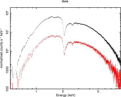
Figure 2 shows two simulated spectra for parameters of model B and two different assumed unabsorbed fluxes - $f_{2-10keV}=4.42\times 10^{-10}\,$erg cm${}^{-2}\,$s^-1 (black crosses) and $f_{2-10keV}=4.41\times 10^{-11}\,$erg cm${}^{-2}\,$s^-1 (red). In case of spectrum with larger flux, for a 1 second exposure time, we have collected 2.36$\times 10^{6}$ photons, enough to obtain our science goal.

4 FITTING PROCEDURES

Our method of determination of neutron star parameters is based on the fitting of theoretical spectra to the observed one – in this case to the WFI/ATHENA fake spectrum. We used the fake data with higher unabsorbed flux (black crosses at Fig. 2) for further analysis.

Figure 3: Top panel: data (fake spectrum B) and our best fit model, while bottom panel shows residua (data minus the folded model). Parameters of the fit are as follow: $T_{\rm eff}=2.18\times 10^{7}\,$K, log(g)=14.28, z=0.305, $N_{ATM}=2.56\times 10^{-24}$ and $N_{\rm H}=0.804\times 10^{22}\,$cm^-2 and $\chi^{2}$=518.52/869.

The theoretical models used do fit the fake spectrum are constructed for one chemical composition, given above. Four parameters as: effective temperature, surface gravity, gravitational redshift and normalization are free parameters in our fitting procedure. In addition, $T_{\rm eff}$ and $\log g$ are input parameters in our atmospheric ATM24 numerical simulations. We calculated an extensive grid of theoretical spectra (nearly 5000 models) with the chemical composition given above. In our initial grid of models, the effective temperature ranges from $10^{7}$ K to $2.70\times 10^{7}\,$K with step $\Delta T_{\rm eff}=0.02\times 10^{7}\,$K, surface gravity $\log g$ from the critical gravity up to 15.0 (cgs) with $\Delta\log g=0.02$. However, we found that the error of $\log g$ is smaller than $\Delta\log=0.02$, so it was obvious that we needed a denser grid of models. Thus, we have chosen smaller steps of parameters around our reference values for the effective temperature and gravity. For the effective temperatures in the range from $T_{\rm eff}=2.18\times 10^{7}\,$K to $2.22\times 10^{7}\,$K steps were $\Delta T_{\rm eff}=0.01\times 10^{7}\,$K, and for surface gravity ranging from $\log g=13.9$ to $14.60$ we have chosen $\Delta\log g=0.01$. All our models were converted to FITS format (Wells et al., 1981), suitable to xspec 12.6.0 package (Arnaud, 1996). The latter software was used also to fit our models to simulated WFI/ATHENA spectrum.

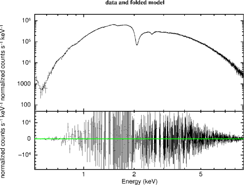
For each given combination of values of $T_{\rm{eff}}$ and $\log(g)$, the surface redshift $z$ was varied from 0.1 to 0.6 with steps of 0.005. The value of model normalization factor $N_{\rm ATM}$ corresponding to the best fit was determined. During the fitting procedure the value of hydrogen column density ($N_{H}$) in model of Galactic absorption (tbabs model in xspec) was a free parameter. Therefore, we obtained a large, 5-dimensional table of $\chi^{2}$ for one assumed chemical composition. Then, from this huge table, we extracted one set of four parameters ($T_{\rm eff}$, $\log{(g)}$, $z$ and $N_{\rm ATM}$) corresponding to the fit with the lowest value of $\chi^{2}$. We found also 1, 2 and 3$\sigma$ confidence levels in $\log(g)-z$ parameters space, requiring that $\chi^{2}_{\rm min}<\chi^{2}<\chi^{2}_{\rm min}+\Delta\chi^{2}$, and additionally that $0.1<M<3\,$M_⊙. The value of $\Delta\chi^{2}$ corresponds to the 1, 2 and 3$\sigma$ confidence levels for two free parameters (Press et al., 1992). The best fitted model and residua are presented in Figure 3.

Table 2: Best fit parameters and 1$\sigma$ and 2$\sigma$ errors (in parenthesis).

fake spectrum A
$N_{H}$		log(g)		z		M[M⊙]		R[km]
0.802	${}^{+0.002}_{-0.002}(^{0.004}_{0.004})$	14.26	${}^{+0.03}_{-0.02}$(${}^{+0.03}_{-0.03}$)	0.255	${}^{+0.005}_{-0.020}$(${}^{+0.020}_{-0.025}$)	1.40	${}^{+0.05}_{-0.15}$(${}^{+0.20}_{-0.24}$)	11.32	${}^{+0.32}_{-0.94}$ (${}^{+1.24}_{-1.32}$)
fake spectrum B
0.804	${}^{+0.002}_{-0.002}(^{0.004}_{0.004})$	14.28	${}^{+0.04}_{-0.0005}(^{+0.06}_{-0.01})$	0.305	${}^{+0.015}_{-0.010}(^{+0.025}_{-0.015})$	1.78	${}^{+0.05}_{-0.13}(^{+0.18}_{-0.25})$	12.71	${}^{+0.19}_{-0.95}(^{+0.87}_{-1.64})$
fake spectrum C
0.800	${}^{+0.002}_{-0.002}(^{0.004}_{0.003})$	14.32	${}^{+0.04}_{-0.02}(^{+0.06}_{-0.03})$	0.360	${}^{+0.015}_{-0.015}(^{+0.030}_{-0.025})$	2.09	${}^{+0.15}_{-0.22}(^{+0.24}_{-0.31})$	13.44	${}^{+0.99}_{-1.08}(^{+1.32}_{-1.88})$

Table 3: Best fitted parameters for our three fake spectra, A, B and C. Confidence values for 1$\sigma$, 2$\sigma$ and 3$\sigma$ are given in next three rows for each model.

fake spectrum A
	$z$	$\log(g)$ [cgs]	$M$ [M⊙]	$R$ [km]
best par.	0.255	14.26	1.399	11.315
1$\sigma$	0.235 – 0.260	14.24 – 14.29	1.252 – 1.444	10.371 – 11.637
2$\sigma$	0.230 – 0.275	14.23 – 14.29	1.155 – 1.595	9.992 – 12.556
3$\sigma$	0.220 – 0.258	14.22 – 14.31	1.049 – 1.711	9.392 – 13.068
fake spectrum B
	$z$	$\log(g)$ [cgs]	$M$ [M⊙]	$R$ [km]
best par.	0.305	14.28	1.776	12.705
1$\sigma$	0.295 – 0.320	14.28 – 14.32	1.647 – 1.825	11.758 – 12.892
2$\sigma$	0.290 – 0.330	14.27 – 14.34	1.531 – 1.959	11.066 – 13.573
3$\sigma$	0.280 – 0.335	14.26 – 14.35	1.429 – 2.054	10.494 – 14.083
fake spectrum C
	$z$	$\log(g)$ [cgs]	$M$ [M⊙]	$R$ [km]
best par.	0.360	14.32	2.090	13.437
1$\sigma$	0.345 – 0.375	14.30– 14.36	1.869 – 2.235	12.230 – 14.243
2$\sigma$	0.335 – 0.390	14.29 – 14.38	1.782 – 2.334	11.558 – 14.752
3$\sigma$	0.325 – 0.395	14.28 – 14.40	1.630 – 2.486	10.761 – 15.456

5 RESULTS

As a result of fitting the simulated WFI/ATHENA data we determined the effective temperature $T_{\rm eff}$, surface gravity $\log g$ and gravitational redshift $z$. The two latter parameters are converted into mass and radius of the neutron star following Majczyna & Madej (2005):

$$R=\frac{zc^{2}}{2g}\frac{(2+z)}{(1+z)},$$ (3)

and

$$M=\frac{z^{2}c^{4}}{4gG}\frac{(2+z)^{2}}{(1+z)^{3}},$$ (4)

where $G$ is the gravitational constant and $c$ is the speed of light.

Figure 4: 1, 2 and 3$\sigma$ confidence contours for two free parameters: redshift and surface gravity for three models A – left panel, B – middle panel, and C – right panel. Black cross denotes our reference values, while black dot is the best fitted value.

Figure 5: 1, 2 and 3$\sigma$ confidence contours for two free parameters: mass and radius for model A. Right panel is the enlarged version of the left panel. Black point denotes our best fit mass and radius values $M=1.399\,$M_⊙ and $R=11.315\,$km, whereas black cross denotes our reference values. Thin gray lines represent possible EOS solutions (Haensel et al., 2007)

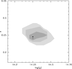
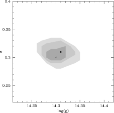
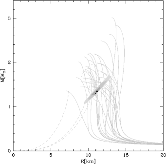
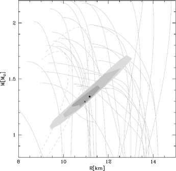
Table 2 contains our best fit parameters and the accuracy of their determination obtained by using of our method. Errors were defined as 1$\sigma$ and 2$\sigma$ standard deviations (in parenthesis). The goal of our fitting procedure is to reproduce assumed values of the parameters for which the fake spectrum was calculated (see Sec. 3). We obtained best fit parameters that differ slightly from the assumed values, but the difference is less than 1$\sigma$ standard deviations. Values of 1, 2 and 3$\sigma$ confidence ranges determined for two free parameters, are presented in Table 3, where the minimum $\chi^{2}$ corresponds to parameters of the neutron star that differ slightly from the assumed values

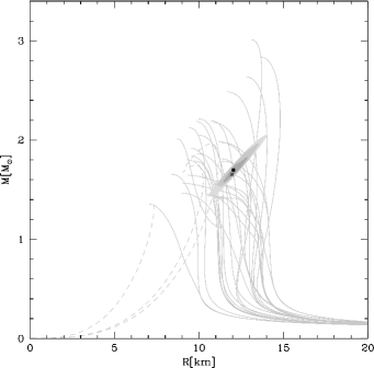
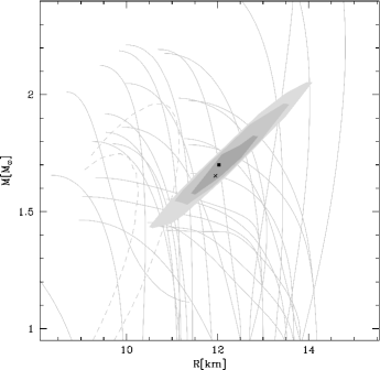
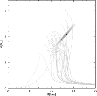
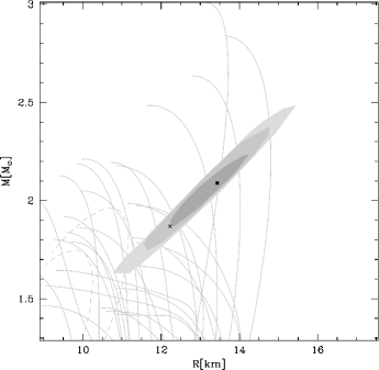
Figure 4 shows the 1,2 and 3$\sigma$ confidence contours, which are obtained for two free parameters: redshift and surface gravity, for all models. On this figure, the black cross denotes the best fitted value of those parameters. The input assumed values were denoted as black dot. In all cases, fitted values are within 1$\sigma$ confidence contours. Corresponding masses and radii for models A, B and C, are presented in Figures 5, 6, and 7, respectively. Furthermore, the grey lines denote possible EOS solutions in those figures.

Figure 6: 1, 2 and 3$\sigma$ confidence contours for two free parameters: mass and radius for model B. Right panel is the enlarged version of the left panel. Black point denotes our best fit mass and radius values $M=1.776\,$M_⊙ and $R=12.705\,$km, whereas black cross denotes our reference values. Thin grey lines represent possible EOS solutions (Haensel et al., 2007)

Figure 7: 1, 2 and 3$\sigma$ confidence contours for two free parameters: mass and radius for model C. Right panel is the enlarged version of the left panel. Black point denotes our best fit mass and radius values $M=2.090\,$M_⊙ and $R=13.437\,$km, whereas black cross denotes our reference values. Thin grey lines represent possible EOS solutions (Haensel et al., 2007)

6 SUMMARY

Determination of basic parameters of neutron stars is very important for the derivation of the equation of state of superdense matter. In this paper, we presented the method of mass and radius determination for neutron stars. Our method is based on the fitting of theoretical spectra to the observed one. Importantly, our method is independent on the distance, which is proportional to the normalization of the model. This is because the normalization factor $N_{\rm ATM}$ is the result of our fitting procedure. Therefore, the knowledge of the distance to the source is not necessary if we determined neutron star parameters with our method. Figure 1 shows our theoretical spectra for two very different chemical compositions. Shape of the continuum of these spectra is different as well as the location of its maxima. Those differences indicate, that even tentative knowledge of the chemical composition is crucial for our method. In case of many neutron stars the chemical composition of their atmospheres is known (eg. Goodwin et al. (2019)).

We calculated a large grid of theoretical spectra of hot neutron star using ATM24 code. assuming effective temperatures $T_{\rm eff}=(1.5-2.7)\times 10^{7}\,$K, logarithm of gravity from 15.0 down to the critical value, and chemical abundances as defined in Section 4. Parameters of models in the grid changed with steps of $\Delta T_{\rm eff}=0.02\times 10^{7}\,$K and $\Delta\log(g)=0.02$; chemical composition was kept the same for all models.

Our goal was to determine the precision of mass and radius determination of the neutron star, based on the spectra to be obtained with the WFI/ATHENA instrument. Due to lack of real ATHENA observations, we simulated three spectra using publicly available WFI calibration files. We constructed three fake spectra A, B, and C corresponding to three different values of effective temperatures, surface gravities and redshifts. We have chosen normalization factors $N_{\rm ATM}$ which correspond to the observed fluxes of a few hundredths of the Crab ($\sim 10^{-10}\,$erg cm${}^{-2}\,$s^-1). ATHENA instrument systematic errors on the level of 3% were taken into account where simulated spectra were created.

Next, we fitted these fake spectra by a large grid of our theoretical spectra. We obtained the best fit ($1\sigma$) for the following parameters of fake spectra: A $M=1.40^{+0.05}_{-0.15}\,$M_⊙ and $R=11.32^{+0.32}_{-0.94}\,$km, B $M=1.78^{+0.05}_{-0.13}\,$M_⊙ and $R=12.71^{+0.19}_{-0.95}\,$km, C $M=2.09^{+0.15}_{-0.22}\,$M_⊙ and $R=13.44^{+0.99}_{-1.08}\,$km, and the corresponding masses and radii for 3$\sigma$ confidence ranges $M=1.05-1.71\,$M_⊙ and $R=9.38-13.07\,$km, $M=1.43-2.05\,$M_⊙ and $R=10.49-14.08\,$km, $M=1.63-2.49\,$M_⊙ and $R=10.76-15.46\,$km, respectively.

In each above case we determined precision of the mass and radius measurement with errors in the range 3–10% for mass and in the range 2–8% for radius within the one sigma confidence error. All errors ($1\sigma$) are relatively small for the WFI/ATHENA detector. We note that the errors defined by 2$\sigma$ confidence ranges are in the range 11–17%. Therefore, we showed that our method allows one to constrain the equation of state of dense matter which comprises neutron stars using future observations of ATHENA mission.

References

- Antoniadis et al. (2013) Antoniadis, J., Freire, P. C. C., Wex, N., et al. 2013, Science, 340, 448, doi: 10.1126/science.1233232
- Arnaud et al. (2011) Arnaud, K., Smith, R., & Siemiginowska, A. 2011, Handbook of X-ray Astronomy
- Arnaud (1996) Arnaud, K. A. 1996, in Astronomical Society of the Pacific Conference Series, Vol. 101, Astronomical Data Analysis Software and Systems V, ed. G. H. Jacoby & J. Barnes, 17
- Barret et al. (2013) Barret, D., den Herder, J. W., Piro, L., et al. 2013, ArXiv e-prints. https://arxiv.org/abs/1308.6784
- Demorest et al. (2010) Demorest, P. B., Pennucci, T., Ransom, S. M., Roberts, M. S. E., & Hessels, J. W. T. 2010, Nature, 467, 1081, doi: 10.1038/nature09466
- Galloway & Keek (2017) Galloway, D. K., & Keek, L. 2017, arXiv e-prints, arXiv:1712.06227. https://arxiv.org/abs/1712.06227
- Goodwin et al. (2019) Goodwin, A. J., Galloway, D. K., in’t Zand, J. J. M., et al. 2019, MNRAS, 486, 4149, doi: 10.1093/mnras/stz1094
- Guilbert (1981) Guilbert, P. W. 1981, MNRAS, 197, 451, doi: 10.1093/mnras/197.2.451
- Haensel et al. (2007) Haensel, P., Potekhin, A. Y., & Yakovlev, D. G. 2007, Neutron Stars I. Equation of State and Structure
- Hewish et al. (1968) Hewish, A., Bell, S. J., Pilkington, J. D. H., Scott, P. F., & Collins, R. A. 1968, Nature, 217, 709, doi: 10.1038/217709a0
- Kuśmierek et al. (2011) Kuśmierek, K., Madej, J., & Kuulkers, E. 2011, MNRAS, 415, 3344, doi: 10.1111/j.1365-2966.2011.18948.x
- Lee et al. (2011) Lee, H., Kashyap, V. L., van Dyk, D. A., et al. 2011, ApJ, 731, 126, doi: 10.1088/0004-637X/731/2/126
- Madej (1989) Madej, J. 1989, ApJ, 339, 386, doi: 10.1086/167304
- Madej (1991) Madej, J. 1991, ApJ, 376, 161, doi: 10.1086/170264
- Madej et al. (2017) Madej, J., Różańska, A., Majczyna, A., & Należyty, M. 2017, MNRAS, 469, 2032, doi: 10.1093/mnras/stx994
- Majczyna & Madej (2005) Majczyna, A., & Madej, J. 2005, AcA, 55, 349
- Majczyna et al. (2005) Majczyna, A., Madej, J., Joss, P. C., & Różańska, A. 2005, A&A, 430, 643, doi: 10.1051/0004-6361:20034048
- Medin et al. (2016) Medin, Z., von Steinkirch, M., Calder, A. C., et al. 2016, ApJ, 832, 102, doi: 10.3847/0004-637X/832/2/102
- Nandra et al. (2013) Nandra, K., Barret, D., Barcons, X., et al. 2013, ArXiv e-prints. https://arxiv.org/abs/1306.2307
- Özel et al. (2009) Özel, F., Güver, T., & Psaltis, D. 2009, ApJ, 693, 1775, doi: 10.1088/0004-637X/693/2/1775
- Pomraning (1973) Pomraning, G. C. 1973, The equations of radiation hydrodynamics
- Press et al. (1992) Press, W. H., Teukolsky, S. A., Vetterling, W. T., & Flannery, B. P. 1992, Numerical recipes in FORTRAN. The art of scientific computing
- Rau et al. (2013) Rau, A., Meidinger, N., Nandra, K., et al. 2013, ArXiv e-prints. https://arxiv.org/abs/1308.6785
- Sampson (1959) Sampson, D. H. 1959, ApJ, 129, 734, doi: 10.1086/146671
- Suleimanov et al. (2011) Suleimanov, V., Poutanen, J., & Werner, K. 2011, A&A, 527, A139, doi: 10.1051/0004-6361/201015845
- Suleimanov et al. (2017) Suleimanov, V. F., Kajava, J. J. E., Molkov, S. V., et al. 2017, MNRAS, 472, 3905, doi: 10.1093/mnras/stx2234
- Vincent et al. (2018) Vincent, F. H., Bejger, M., Różańska, A., et al. 2018, ApJ, 855, 116, doi: 10.3847/1538-4357/aab0a3
- Watts et al. (2016) Watts, A. L., Andersson, N., Chakrabarty, D., et al. 2016, Reviews of Modern Physics, 88, 021001, doi: 10.1103/RevModPhys.88.021001
- Wells et al. (1981) Wells, D. C., Greisen, E. W., & Harten, R. H. 1981, A&AS, 44, 363
- Xu et al. (2014) Xu, J., van Dyk, D. A., Kashyap, V. L., et al. 2014, ApJ, 794, 97, doi: 10.1088/0004-637X/794/2/97