Inferring HIV incidence trends and transmission dynamics with a spatio-temporal HIV epidemic model

Abstract

Reliable estimation of spatio-temporal trends in population-level HIV incidence is becoming an increasingly critical component of HIV prevention policy-making. However, direct measurement is nearly impossible. Current, widely used models infer incidence from survey and surveillance seroprevalence data, but they require unrealistic assumptions about spatial independence across spatial units.

In this study, we present an epidemic model of HIV that explicitly simulates the spatial dynamics of HIV over many small, interacting areal units. By integrating all available population-level data, we are able to infer not only spatio-temporally varying incidence, but also ART initiation rates and patient counts. Our study illustrates the feasibility of applying compartmental models to larger inferential problems than those to which they are typically applied, as well as the value of “data fusion” approaches to infectious disease modeling.

 

Introduction

Fitting population-level models of the human immunodeficiency virus (HIV) epidemic to a combination of survey and surveillance data is an essential component of HIV policymaking (Stover et al. 2017). HIV is most prevalent in countries with limited capacity for health surveillance, so data are relatively sparse in the places where we need it most. We use models to fill in the gaps and estimate the indicators we need in order to assess the epidemic’s trajectory (Brown et al. 2014). These indicators include things like adult HIV prevalence, HIV incidence, and coverage of life-saving antiretroviral treatment (ART) (“Monitoring, Evaluation, and Reporting (MER 2.0) Indicator Reference Guide” 2017).

Recently, improved data collection and expanded computational power have increased demand for indicators at subnational levels (Meyer-Rath et al. 2018). We have the data and models to produce reliable maps of HIV prevalence, but similar deep thought has not been given to inferring HIV incidence over space (Dwyer-Lindgren et al. 2019; Cuadros et al. 2017; Gutreuter et al. 2019).Existing methods for inferring HIV inference invariably treat each spatial unit as separate from all others (Brown et al. 2014; Stover et al. 2017), an obviously incorrect assumption. This is more than a theoretical concern. If we were to enact a truly effective HIV prevention programme in an urban area and evaluate it without taking into account the new infections prevented in surrounding suburban areas, we could easily underestimate our programme’s efficacy.

Our goal is to develop a model of HIV that can infer incidence over space, as well as time. It must offer estimates at useful geographic resolutions without incurring extreme computational costs. In this technical report, we will provide a detailed account of our progress towards this end.

First, we will outline the available population-level data sources that might inform estimates of HIV incidence and distributional assumptions we could use to integrate these data into a statistical model. Then, we will describe the mechanistic model we are using to project the HIV epidemic given a set of inferred parameters. Finally, we will provide preliminary estimates from an application to Malawi and a summary of our findings thus far.

Methodology

Because a new HIV infection might not be detected for several years, incidence is virtually impossible to observe directly. Instead, we can use mechanistic models to “fuse” together what indicators we do have and infer the incidence series that was most likely to have generated the combined observed dataset. This is the principle of data fusion (Hall and Llinas 1997). In this section, we will first describe and develop notation for types of data used in our analysis and propose distributional assumptions that we believe represent the generation processes of those data. Then we will describe our compartmental model of HIV in detail.

Data and Distributional Assumptions

We have identified three measurable indicators that will allow us to infer HIV incidence: prevalence, ART coverage, and the proportion of infections at a given time classified as “recent.”

Prevalence

HIV antibody assay results are far and away the most prevalent and reliable source of population-level HIV data. They come from two main sources: large, nationally representative household surveys and routine surveillance at antenatal care (ANC) clinics. These assays give us seroprevalence data consisting the number of tests conducted in a given group and the number of those tests that were positive. Let $r$ and $t$ represent a geographic region and point in time, respectively. Then for a given data source, $s$, we can denote the number of tests in region $r$ at time $t$ as $T_{r,t}^{s,\text{HIV}}$ and the number of positive tests as $P_{r,t}^{s,\text{HIV}}$. Here, $s$ represents either a specific survey or a specific antenatal care site.

We assume that large household surveys are representative for every region, so if $s$ is a household survey, $P_{r,t}^{s,\text{HIV}}/T_{r,t}^{s,\text{HIV}}$ provides an unbiased estimate of true prevalence in demographic segment $\{r,t\}$, denoted $\rho_{r}(t)$. Therefore, we can assume that $P_{r,t}^{s,\text{HIV}}$ is a sample from a binomial distribution with $T_{r,t}^{s,\text{HIV}}$ trials each with a probability of $\rho_{r}(t)$:

$$P^{s,\text{HIV}}_{r,t}\sim\text{Binom}(T_{r,t}^{s,\text{HIV}},\rho_{r}(t))$$ (1)

These surveys are the most reliable data source we have for HIV prevalence, but they are expensive and relatively infrequent. We might have two or three surveys over the past 10 years in any given sub-Saharan African nation.

On the other hand, ANC clinics report data regularly but are attended exclusively by pregnant women, who we might expect to be at differential risk of HIV infection relative to the general population. Therefore, we cannot estimate $\rho_{r}(t)$ with $P^{s,\text{HIV}}_{r,t}/T^{s,\text{HIV}}_{r,t}$ with. Instead, following Bao (2012), We estimate site-specific ANC prevalence as a function of general population prevalence and clinic effects:

$$\begin{split}\text{logit}\;\rho^{s}_{r}(t)&=\text{logit}\;\rho_{r}(t)+\delta_{s}\\ \delta_{s}&\sim\text{N}(0,\sigma^{2}_{\delta})\\ \sigma^{2}_{s}&\sim\text{N}^{+}(0,1)\end{split}$$ (2)

where $\delta_{s}$ is a clinic-specific intercept. Then we can proceed as above:

$$P^{s,\text{HIV}}_{r,t}\sim\text{Binom}(T_{r,t}^{s,\text{HIV}},\rho^{s}_{r}(t)).$$ (3)

ANC clinic HIV test results are less representative and more susceptible to collection error than survey data, but they are available at far greater temporal frequency.

Treatment

Several of the most recent household surveys conducted assays for the presence of antiretroviral treatment (ART) in HIV-positive respondents’ blood samples.(ICAP at Columbia University and PEPFAR 2019) Let $T_{r,t}^{s,\text{ART}}$ represent the number of people tested for ART, and let the $P_{r,t}^{s,\text{HIV}}$ be the number of positive tests. As above, we assume that these seroprevalence data provide an unbiased estimate of true ART coverage in population segment $\{r,t\}$, denoted $\alpha_{r}(t)$. Then we can make the same assumption as before:

$$P^{s,\text{ART}}_{r,t}\sim\text{Binom}(T_{r,t}^{s,\text{ART}},\alpha_{r}(t)).$$ (4)

Programmatic Patient Count Data

Because government-run clinics represent the largest administrators of ART in most high-prevalence areas, we have an additional source of data on ART coverage: facility-level ART patient counts. For a given facility, we have the number of ART patients that facility treated over a given time span (often quarterly intervals), which we will denote $C^{s}_{r,t}$. For convenience, we are currently using counts aggregated to the region level: $C_{r,t}$.

Given that we cannot measure the denominators for these data and that they represent a nearly complete count of the number of adults receiving ART in segment a given region at a given time, we need to model them as count data. If we are willing to assume that the share of people on ART who receive treatment outside of government run clinics is negligibly small, then we can assume that $C_{r,t}$ is an unbiased measurement of the true number of adults on treatment at time $t$ in region $r$, denoted $A_{r}(t)$.

A Likelihood for Varying Population Sizes

Fitting a model to these counts is a trickier problem that it might seem. All else being equal, we would expect a large urban region to serve more ART patients than a small rural region, so we need a model that will make assumptions about variance that can work across regions of varying population sizes.

Following Lindén and Mäntyniemi (2011), we have implemented a negative binomial model with a variance that can scale both linearly and quadratically with its mean. Say we are using the standard negative binomial parameterization:

$$Pr(X=x;r,p)=\frac{\Gamma(x+r)}{x!\Gamma(r)}p^{r}(1-p)^{x}.$$ (5)

Then $\mathbb{E}(X)=\mu=r(1-p)/p$ and $\text{Var}(X)=\sigma^{2}=r(1-p)/p^{2}$. We can solve for $r$ and $p$ to see that $r=\mu^{2}/(\sigma^{2}-\mu)$ and $p=\mu/\sigma^{2}$. In a traditional negative binomial model with $\mu<\sigma^{2}$, we estimate an overdispersion parameter, $\theta>0$, and define

$$\sigma^{2}=\mu+\theta\mu^{2}.$$ (6)

As $\theta\to 0$, $\sigma^{2}\to\mu$ and the distribution converges to a Poisson distribution with rate parameter $\mu$.

With this formulation, we can see why fitting a model simultaneously to regions of varying size might be difficult. A single value of $\theta$ will impact regions of different sizes in radically different ways. A lower value of $\theta$ might explain the variation in a large region well, while not adequately accounting for overdispersion in a small region.

To help ease these problems, we use the formulation from Lindén and Mäntyniemi (2011):

$$\sigma^{2}=\mu+\omega\mu+\theta\mu^{2},$$ (7)

where $\theta,\omega>0$. The addition of a linear term should help avoid larger regions blowing smaller regions out of the water, so to speak. Given fixed $\theta$ and $\mu$, as $\omega\to 0$, this distribution converges to a traditional negative binomial with overdispersion $\theta$. Conversely, given fixed $\omega$ and $\mu$, as $\theta\to 0$, it converges to a “quasi-Poisson” distribution. We will write this three-parameter version of the negative binomial distribution as $\text{NegBinom}(\mu,\omega,\theta)$ assuming that $\sigma^{2}$ (and consequently $r$ and $p$) is calculated internally.

Cross-Region Treatment Seeking

The other critical problem we need to address when dealing with these data are that they are collected from facilities, not households. Patients can (and do) seek treatment outside of their regions-of-residence (or “home regions”), so we need to consider that the observed patient count series for a given region is composed of patients from all sufficiently “close” regions. For now, we will say any two regions $j$ and $r$ are sufficiently close if they are within some fixed degree of adjacency of each other (the number of borders we need to cross to get from $r$ to $j$ is less than $D$). The results presented below were generated by a model with $D=2$. Let $j\sim r$ denote $j$ and $r$ being adjacent, and let $\{k\sim r\}$ be the set of all regions that are “close” to $r$.

We can define a multinomial model for the odds that an individual with home region $r$ will seek treatment in adjacent district $j$ over region $r$:

$$\begin{split}\text{log}\;\frac{P(A_{r\to j})}{P(A_{r\to r})}&=\frac{\text{log}\;m_{j}}{d_{i\to j}^{2}}\\ \text{log}\;m_{j}&\sim\text{N}(\text{log}\;\bar{m}_{j},\sigma_{m})\\ \sigma_{m}&\sim\text{N}^{+}(0,1)\\ \bar{m}_{j}&=\frac{0.05}{\|\{k\sim j\}\setminus j\|}\end{split}$$ (8)

where $m_{j}$ is a destination-specific intercept and $d_{i\to j}$ is the number of borders needed to cross to get from $i$ to $j$. Note that $P(A_{r\to r})/P(A_{r\to r})=m_{r}=1$, so we do not need a model for each home region. We are currently defining the prior mean for each $m_{j}$ as $0.05$ divided by the number of regions for which $j$ is a neighbor within $D$ degrees, which is exactly $\{k\sim j\}\setminus j$. Roughly speaking, this means that we expect 5% of ART patients in any region $r$ to seek treatment outside of $r$. For all $j\sim r$ (including $r$ itself), we can find

$$P(A_{r\to j})=\pi_{r\to j}=\frac{{m_{j}}}{\sum_{l\in\{k\sim r\}}{m_{l}}}.$$ (9)

With $\pi_{r\to j}$, we can allocate the total count of people receiving treatment in $r$ to each $j\sim r$. We can estimate the total number of people receiving treatment in $r$ as

$$A^{\star}_{r}(t)=\sum_{j\in\{k\sim r\}}\pi_{j\to r}A_{j}(t).$$ (10)

Note that we are using $\pi_{j\to r}$ inside the summand, not $\pi_{r\to j}$; we are essentially collecting all of the ART patients in $j$ we believe are going from $j$ to $r$ to find the total number of patients receiving treatment in $r$.

At long last, we can define a likelihood for the ART patient count data. Using the three-parameter negative binomial parameterisation from before, we have

$$\begin{split}C_{r,t}&\sim\text{NegBinom}(A^{\star}_{r}(t),\omega,\theta)\\ \text{log}\;\omega&\sim\text{N}(0,2)\\ \text{log}\;\theta&\sim\text{N}(0,2),\end{split}$$ (11)

where $\text{log}\;\omega$ and $\text{log}\;\theta$ are estimated parameters. The priors on $\omega$ and $\theta$ are essentially arbitrary and could certainly be improved. In a sense, we are fitting a multinomial model on a matrix of flow counts for which we only observe one set of margins.

Recency

Our final source of data is recency assays from the most recent wave of household surveys (those conducted as a part of the PHIA program). These data offer estimates of the proportion of people living with HIV (PLHIV) who were infected in the past year, the closest thing to direct incidence measurement available. Reusing the notation from the other seroprevalence data sources, we have $P_{r,t}^{s,\text{Rec}}$ and $T_{r,t}^{s,\text{Rec}}$. If we know the HIV incidence and prevalence rates in a given demographic segment, $\lambda_{r}(t)$ and $\rho_{r}(t)$ respectively, we can use the estimator from Kassanjee, McWalter, and Welte (2014) to find the implied proportion of infections that should be recent:

$$\nu_{r}(t)=\frac{\lambda_{r}(t)\cdot(1-\rho_{r}(t))\cdot(\Omega_{R}-\gamma_{R})+\gamma_{R}\rho_{r}(t)}{\rho_{r}(t)},\\$$ (12)

where $\Omega_{R}$ is the mean duration of recent infection (fixed at 130/365), and $\gamma_{R}$ is the proportion of positive recency assays that are false positives (fixed at 0).

As before, we assume that each $P_{r,t}^{s,\text{Rec}}$ is a sample from a binomial distribution:

$$P^{s,\text{Rec}}_{r,t}\sim\text{Binom}(T_{r,t}^{s,\text{Rec}},\nu_{r}(t)).$$ (13)

Although these data are the closest thing we have to direct measurement of population-level incidence, they typically do not contain enough information to be useful. For example, the recent MPHIA survey in Malawi returned at least one positive recency assays in only nine of Malawi’s 28 districts.

Inference Problem

As we have seen, none of the available data measure incidence directly, but they are all generated from the same global HIV epidemic. Therefore, if we can construct a model that estimates incidence and finds the implied values of the measurable indicators, we can infer incidence. More formally, say we are interested in estimation for a set of regions, $\{r_{1},...,r_{R}\}$ and extent of time $[t_{1},t_{T}]$. For convenience, let $r$ and $t$ be arbitrary elements in $\{r_{1},...,r_{R}\}$ and $[t_{1},t_{T}]$, respectively. Then, our goal is to infer a matrix $\Lambda$ where $\Lambda_{(r,t)}=\lambda_{r}(t)$ given all available, relevant data $\mathcal{D}$; that is, we want to estimate $P(\Lambda\;|\;\mathcal{D})$ where $\mathcal{D}$ is the collation of all indicators described in the previous section. Keeping with previous literature (Brown et al. 2014, for example), our epidemic model will be deterministic, so we know that $P(\Lambda\;|\;\mathcal{D})=P(\theta\;|\;\mathcal{D})$. Therefore, we can use classical Bayesian inference:

$$P(\theta\;|\;\mathcal{D})\propto P(\mathcal{D}\;|\;\theta)P(\theta).$$ (14)

Within this framework, we need to define two components: a likelihood $P(\mathcal{D}\;|\;\theta)$ and a prior distribution $P(\theta)$. We have already defined the likelihood and priors for the observation model with the distributional assumptions described above. In the next section, we will describe the mechanistic model needed to relate $\Lambda$ to $\mathcal{D}$ and the priors required to identify that model.

Epidemic Model

We have made a set of distributional assumptions about the relationships between three data sources (surveys, surveillance, and programmatic counts) and the true, underlying HIV epidemic. To actually calculate $P(\mathcal{D};\theta^{\star})$ for a given candidate set of parameters $\theta^{\star}$ we need to estimate the underlying epidemic. Specifically, we need estimates of, prevalence, ART coverage, ART patient counts, and incidence ($\rho_{r}(t)$, $\alpha_{r}(t)$, $A_{r}(t)$, and $\lambda_{r}(t)$, respectively).

Compartmental Models

Compartmental models give us a way to build a generative model of the disease indicators we need. Our model is essentially a variation of the classical susceptible-infectious-recovered (SIR) model of infectious disease. We track the populations in several mutually exclusive and comprehensive compartments and define a system of ordinary differential equations (ODEs) to govern rates of movement from one compartment to another.

For example, the classical SIR model measures the number of susceptible, infectious, and recovered individuals ($S(t)$, $I(t)$, and $R(t)$, respectively) in a closed population. Let $N(t)=S(t)+I(t)+R(t)$ be the size of the population at time $t$. We can assume that infectious individuals move from $I$ to $R$ according to some recovery rate $\gamma\in\mathbb{R}^{+}$. Further, if we assume the principle of mass action holds, we can assume that individuals move from $S$ to $I$ in proportion to the size of $I$ according to a transmission rate $\kappa\in\mathbb{R}^{+}$. Then we can define the whole model:

$$\begin{split}\frac{\partial S(t)}{\partial t}&=-\kappa S(t)I(t)/N(t)\\ \frac{\partial I(t)}{\partial t}&=\kappa S(t)I(t)/N(t)-\gamma I(t)\\ \frac{\partial R(t)}{\partial t}&=\gamma I(t).\end{split}$$ (15)

Fixing $\kappa$, $\gamma$, and the initial state of the system, $(S(0),I(0),R(0))$, we can use the numerical method of our choosing to find $(S(t),I(t),R(t))$ for any $t>0$.

In keeping with other work in this area, we are using the forward Euler method, meaning we will be discretising the domain of the system of ODEs (in this case, time) into intervals of length $h$:

$$\begin{split}S(t+h)&=S(t)+h\cdot(-\kappa S(t)I(t))\\ I(t+h)&=I(t)+h\cdot(\kappa S(t)I(t)-\gamma I(t))\\ R(t+h)&=R(t)+h\cdot(\gamma I(t)).\end{split}$$ (16)

If we define $h$ to be some percentage of a calendar year, we can view this as a discrete-time SIR model where $h$ scales per-person-year rates to a timescale of our choice.

Epidemic Model of HIV

Baseline Model

For many reasons, this simple SIR model is not suited for HIV. We will outline a few discrepancies here:

1. Because HIV is a lifelong infection, the size of the $R$ compartment is zero everywhere (ignoring two remarkable cases (Hütter et al. 2009; Gupta et al. 2019)), and so we can drop it.

2. HIV prevalence rates can range far above 25% in some populations (“HIV and AIDS in eSwatini. AVERT” 2015), so we cannot ignore demographic dynamics (non-HIV mortality, migration, and ageing-in to the adult population).

3. Untreated HIV is highly fatal, so we need to account for AIDS-related mortality (Yiannoutsos et al. 2012; Todd et al. 2007; Marston et al. 2007).

4. Good adherence to ART drastically reduces infectiousness, so assuming that risk of infection is constant across contacts with all PLHIV regardless of treatment status will lead to biased estimates of incidence. Therefore, we need to add a compartment for people receiving treatment (Fonner et al. 2016).

Integrating these changes into the system of ODEs from before and reformulating how we calculate incidence to reflect the prophylactic effects of ART, we have the following:

$$\begin{split}\frac{\partial S(t)}{\partial t}&=S(t)\cdot(-\lambda(t)-\mu^{S})+E_{t}\\ \frac{\partial I(t)}{\partial t}&=I(t)\cdot(-(\mu^{S}+\mu^{I})-\alpha^{\star}_{t})+\lambda(t)S(t)+\eta A(t)\\ \frac{\partial A(t)}{\partial t}&=A(t)\cdot(-\mu^{S}-\mu^{A}-\eta)+\alpha^{\star}_{t}I(t),\end{split}$$ (17)

where $\mu^{S}$ is non-HIV mortality, $E_{t}$ is the number of new entrants to the population, $\mu^{I}$ and $\mu^{A}$ are HIV-related mortality with and without ART, respectively, $\alpha^{\star}_{t}$ is the time-dependent rate at which PLHIV initiate ART, and $\eta$ is the rate of dropout from ART. We have rewritten incidence as $\lambda(t)=\kappa_{t}\rho(t)(1-\omega\alpha(t))$, where $\rho(t)=I(t)/N(t)$ is population prevalence, $\omega\in[0,1]$ is percent by which ART reduces infectiousness, and $\alpha(t)=A(t)/(I(t)+A(t))$ is ART coverage among all PLHIV. Hence, $\rho(t)(1-\omega\alpha(t))$ is ART-adjusted prevalence. We have also allowed the HIV transmission rate to vary over time.

Incorporating Disease Progression

To more accurately reflect mortality patterns, we break the infected and on-ART compartments into substages, which we will denote as $I_{c}(t)$ and $A_{c}(t)$. Here $c$ indexes something slightly different across the two super-compartments. We track four substages for both $I$ and $A$ defined by a single set of CD4 count intervals: $([0,200),[200,350),[350,500),[500,\infty))$. We are currently defining these compartments with CD4 count thresholds, but we could equally define them with viral load thresholds. These specific thresholds are borrowed from Johnson and Dorrington’s Thembisa model (Johnson and Dorrington 2019).

For the $I$ compartment, $c$ indexes individuals’ current CD4 count, whereas for the $A$ compartment, it indexes the individuals’ CD4 count at treatment initiation. We assume that individuals can “move” from $I_{c}$ to $I_{c+1}$ but not from $A_{c}$ to $A_{c+1}$.

Including these disease progression dynamics in the model, we get

$$\frac{\partial S(t)}{\partial t}= S(t)\cdot(-\lambda(t)-\mu^{S})+E_{t}$$ (18)

$$\frac{\partial I_{c}(t)}{\partial t}= I_{c}(t)\cdot(-(\mu^{S}+\mu_{c}^{I})-\alpha^{\star}_{c,t}-\tau_{c})+\lambda_{c}(t)S(t)+$$

$$\eta A_{c}(t)+\tau_{c-1}I_{c-1}(t)$$

$$\frac{\partial A_{c}(t)}{\partial t}= A_{c}(t)\cdot(-\mu^{S}-\mu_{c}^{A}-\eta)+\alpha^{\star}_{c,t}I(t),$$

where $\tau_{c}$ is the rate of progression from disease stage $c$ to stage $c+1$ for $c$ less than the maximum value. We take our values of $\tau_{c}$ from Johnson and Dorrington (2019) Table 3.1. Note that AIDS-related mortality now varies by disease stage. Figure 1 outlines the structure of this model.

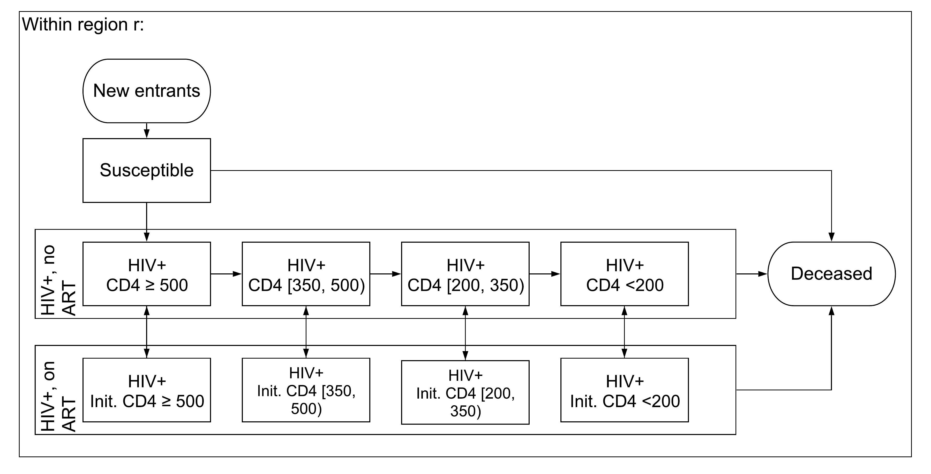
Figure 1: Diagram of our compartmental epidemic model of HIV focused on a single region

Spatial Compartmental Model

Coming back to inferring incidence over space, we can construct a (currently independent) model for each region $r$ and arrive at our final model:

$$\frac{\partial S_{r}(t)}{\partial t}= S_{r}(t)\cdot(-\lambda_{r}(t)-\mu^{S})+E_{r,t}$$ (19)

$$\frac{\partial I_{r,c}(t)}{\partial t}= I_{r,c}(t)\cdot(-(\mu^{S}+\mu_{c}^{I})-\alpha^{\star}_{r,c,t}-\tau_{c})+\lambda_{r,c}(t)S(t)+$$

$$\eta A_{r,c}(t)+\tau_{c-1}I_{r,c-1}(t)$$

$$\frac{\partial A_{r,c}(t)}{\partial t}= A_{r,c}(t)\cdot(-\mu^{S}-\mu_{c}^{A}-\eta)+\alpha^{\star}_{r,c,t}I(t).$$

To project the HIV epidemic and find the indicators we need to evaluate our likelihood, we need models for $\lambda_{r}(t)$, $\alpha^{\star}_{r}(t)$, and $(S_{r}(0),I_{r,c}(0),A_{r,c}(0))$ for all $r$. Because we have not made any structural changes to the model, Figure 1 is still accurate.

If the epidemic in each $r$ were to be perfectly independent from that of all other regions, our previous model of incidence would still be valid. However, this assumption is demonstrably false in a model of infectious disease. HIV first emerged in central Africa in the early 1900s and has since spread to every corner of the globe (Sharp and Hahn 2011); clearly we cannot claim that any two regions contain truly independent epidemics.

We model the spread of disease over space directly by making incidence in region $r$ a function of prevalence in region $r$ and all adjacent regions (again, $\{k\sim r\}$). Specifically, we first model the rate of infections attributable to disease stage $c$ as

$$\log\lambda_{r,c}(t)=\log\kappa_{r,c,t}+\log\sum_{j\in\{k\sim r\}}w(r,j)\rho_{r,c}(t)(1-\omega\alpha_{r,c}(t)),$$ (20)

where $\kappa_{r,c,t}$ is a region-/substage-/time-specific transmission rate, and $w(r,j)$ is a weight proportionate to a measure of distance between $r$ and $j$. Currently, we define $w(r,j)$ such that the share of risk coming from $r$, $w_{0}$, is fixed and the remaining share is divided among its neighbors:

$$w(r,j)=\left\{\begin{aligned} w_{0}\qquad&\qquad r=j\\ \frac{p_{j}(1-w_{0})}{\|\{j\sim r\}\setminus r\|}&\qquad r\neq j,\end{aligned}\right.$$ (21)

where $p_{j}$ is the share of population at time 0 that lives in $j$ among neighbors of $r$. Figure 2 illustrates five assumptions about the degree of spatial connectedness between districts in the Southern region of Malawi relative to the Zomba district.

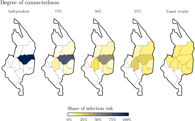
Figure 2: Values of $w(r,j)$ resulting from five assumptions about the degree of connectedness between districts of southern Malawi. Independent assumes that every infection originates internally, whereas "Equal weight" assumes an infection is as likely to come from any of Zomba’s neighbours as from Zomba itself.

We model the log-transformed region-/stage-/time-specific HIV transmission rate $\log\kappa_{r,c,t}$ as a hierarchical b-spline:

$$\begin{array}[]{rl}\text{log}\;\kappa_{r,c,t}&=\log\xi_{c}+\sum_{i=1}^{K_{\kappa}+1}(\beta^{\kappa}_{i,0}+\beta^{\kappa}_{i,r})\phi_{i}(t)\\ \beta^{\kappa}_{i,0}&\sim\text{N}(0,5)\\ \beta^{\kappa}_{i,r}&\sim\text{N}(0,\sigma_{\kappa})\\ \beta^{\kappa}_{i,r}-\beta^{\kappa}_{i-1,r}&\sim\text{N}(0,1)\\ \sigma_{\kappa}&\sim\text{N}^{+}(0,1),\end{array}$$ (22)

where $\xi_{c}$ is the relative infectiousness of stage $c$, $K_{\kappa}$ is the number of knots, $\phi$ is a b-spline basis function of some order, $\beta_{i,0}$ is a mean coefficient for basis function $i$, and $\beta_{i,r}$ is a penalized region-specific coefficient for region $r$. Currently, we place knots at five-year intervals and use a spline of order three. We use the relative infectiousness ratios listed in Table 3.1 in Johnson and Dorrington (2019) to fix the values of $\xi_{c}$.

To obtain the HIV infection rate attributable to all disease stages combined, we convert each $\lambda_{r,c}(t)$ to a probability, $P(\text{inf}_{c};r,t)=1-\exp(-h\cdot\lambda_{r,c}(t))$ assume independence across disease stages, and aggregate as follows:

$$\begin{array}[]{rll}P(\text{not inf}_{c};r,t)&=1-P(\text{inf}_{c};r,t)\\ &=\exp(-h\cdot\lambda_{r,c}(t))\\ \\ P(\text{not inf};r,t)&=P(\cap_{c}\text{not inf}_{c};r,t)\\ &=\prod_{c}P(\text{not inf}_{c};r,t)\\ &=\prod_{c}{\exp(-h\cdot\lambda_{r,c}(t))}\\ \\ P(\text{inf};r,t)&=1-\prod_{c}\exp(-h\cdot\lambda_{r,c}(t))\\ &=1-\exp(-h\sum\limits_{c}\lambda_{r,c}(t))\end{array}$$ (23)

Therefore, assuming the probability of infection from each disease stage is independent from all other stages (that is, that $P(\text{not inf};r,t)=\prod_{c}P(\text{not inf}_{c};r,t)$), the incidence rates are additive. Finally, we can find $\lambda_{r}(t)=1/h\cdot\log P(\text{inf};r,t)$.

Model of ART Initiation

Our model of the ART initiation rate among eligible disease stages is similar to our model of incidence:

$$\begin{array}[]{rl}\text{log}\;\alpha^{\star}_{r,c,t}&=\log\zeta_{c}+\sum_{i=1}^{K_{\alpha}+1}(\beta^{\alpha^{\star}}_{i,0}+\beta^{\alpha^{\star}}_{i,r})\phi_{i}(t)\\ \beta^{\alpha^{\star}}_{i,0}&\sim\text{N}(0,5)\\ \beta^{\alpha^{\star}}_{i,r}&\sim\text{N}(0,\sigma_{\alpha^{\star}})\\ \beta^{\alpha^{\star}}_{i,r}-\beta^{\alpha^{\star}}_{i-1,r}&\sim\text{N}(0,1)\\ \sigma_{\alpha^{\star}}&\sim\text{N}^{+}(0,1).\end{array}$$ (24)

Here, we place a knot every year and set $\phi$ to be order one, essentially making this model a random walk. For all $t$ before ART was scaled up in any region-of-interest, we fix $\phi_{i}(t)$ to be zero; additionally, we do not estimate any $\beta^{\alpha^{\star}}_{i}$ with support entirely before ART scale-up. The model used to generate results presented on December 5th, 2019 fixed $\zeta_{c}=1$ for all eligible $c$, but the latest, less tested version sets $\zeta_{c}=\mu^{I}_{c}/\mu^{I}_{1}$; in other words, PLHIV at stage $c$ initiate treatment in proportion to the expected mortality in $c$.

Estimation of Initial State

Our model can begin the epidemic projection at any point in time by estimating the initial state of the compartmental model, denoted $(S_{r}(0),I_{r,c}(0),A_{r,c}(0))$, with a small area model that draws strength across regions. Specifically, we use logit-linear models to estimate $\rho_{r}(0)$ and $\alpha_{r}(0)$ and use them to solve for $(S_{r}(0),I_{r,c}(0),A_{r,c}(0))$.

Our model for initial prevalence is as follows:

$$\begin{split}\text{logit}\;\rho_{r}(0)&=\rho_{0}+\rho_{r}\\ \rho_{r}&\sim\text{N}(0,\sigma_{\rho})\\ \rho_{0}&\sim\text{N}(0,5)\\ \sigma_{\rho}&\sim\text{N}^{+}(0,1),\end{split}$$ (25)

where $\rho_{0}$ is cross-region logit-transformed prevalence at time $0$ and $\rho_{r}$ is a regional deviation from $\rho_{0}$.

If time 0 is before ART scale-up, $\alpha_{r}(0)$ is fixed to be zero in all regions. Otherwise, we use an equivalent model:

$$\begin{split}\text{logit}\;\alpha_{r}(0)&=\alpha_{0}+\alpha_{r}\\ \alpha_{r}&\sim\text{N}(0,\sigma_{\alpha})\\ \alpha_{0}&\sim\text{N}(0,5)\\ \sigma_{\alpha}&\sim\text{N}^{+}(0,1).\end{split}$$ (26)

Making fixed assumptions about the share of each substage among people with and without treatment, $b^{\alpha}_{c}$ and $b^{\rho}_{c}$, respectively, we can find $I_{r,c}(0)$, $A_{r,c}(0)$, and $S_{r}(0)$:

$$\begin{array}[]{rl}I_{r,c}(0)&=b^{\rho}_{c}\cdot(1-\alpha_{r}(0))\cdot\rho_{r}(0)\cdot P_{r}(0)\\ A_{r,c}(0)&=b^{\alpha}_{c}\cdot\alpha_{r}(0)\cdot\rho_{r}(0)\cdot P_{r}(0)\\ S_{r}(0)&=P_{r}(0)-\sum_{c}(I_{r,c}(0)+A_{r,c}(0)),\end{array}$$ (27)

where $P_{r}(0)$ is exogenously defined population at time $0$ and $b^{\rho}_{c}$ and $b^{\alpha}_{c}$ are fixed assumptions about the share of PLHIV without. Ideally, we would estimate $b^{\rho}_{c}$ and $b^{\alpha}_{c}$, but too few sources provide CD4-specific data for that to be possible. With a model for the initial state, we have everything we need to project the epidemic using our compartmental model.

Implementation

We have implemented this model in C++ using the TMB R/C++ library (Kristensen et al. 2016). This software allows users to write statistical models using the Eigen C++ library (Guennebaud, Jacob, and others 2010) and interact with the compiled models through R. We used the sparse matrix tools built in to Eigen to develop an efficient implementation of the Euler method. Using automatic differentiation, TMB provides access to the gradient functions of arbitrary statistical models and, as such, is a powerful tool for inference and optimization. The inference strategy built in to TMB optimizes the approximate marginal likelihood with respect to a pre-defined set of “random” parameters and, after finding the maximum a posterior (MAP) parameter estimates, assumes the parameters form a multivariate normal distribution around those modes (Kristensen et al. 2016; Skaug and Fournier 2006).

The TMB inference strategy makes extensive use of the Laplace approximation and might therefore be poorly suited to produce samples from distribution that is assymetric, bimodal, or otherwise non-normal. This gap is filled by the tmbstan R package (Monnahan and Kristensen 2018), which uses the objects that TMB builds to run the rstan package’s implementation of No-U-Turn sampler (NUTS) (Carpenter et al. 2017). NUTS is a variant of Hamiltonian Monte Carlo that can reliably produce samples from even extremely complex statistical models and that we believe represents the current gold standard for sampling algorithms. Through tmbstan we can use either inference strategy. The results presented in this paper and at Epidemics 7 were generated from posterior distributions obtained through NUTS.

Application

We fit the model to district-level data from Malawi from the beginning of 2000 to the end of 2018. Between January 1st, 2000 and December 31st, 2018, four nationally representative household surveys collected data on HIV seroprevalence in Malawi: three DHS surveys (2004, 2010, and 2015) (“The DHS Program - DHS Methodology” n.d.) and one PHIA survey (2015-2016) (ICAP at Columbia University and PEPFAR 2019). We used HIV seroprevalence data from each of these surveys, aggregating test results to the district level. The MPHIA survey also provides results of ART and recency blood tests. We incorporated HIV prevalence data from sentinel ANC facilities, of which there are typically two per district, using the hierarchical logistic model described above. Finally, we used reported district-level ART patient counts to inform the model of ART initiation.

Results

The model seems to perform well in applications to data from Malawi, reconciling each of the included data sources without favoring one over another. Figure 3 presents inferred incidence per 1,000 person-years and ART initiaton probabilities as well as fit to data on prevalence and ART patient counts in the Dedza district of Malawi. Because both incidence and underlying ART initiation rates are difficult to measure directly, our ability to assess the validity of our inference is limited. This hinderance is not unique to our study, but it is worth highlighting.

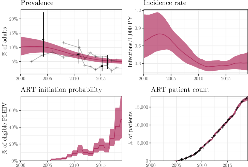
Figure 3: Data and estimates in the Dedza district of Malawi. Circular points and line ranges represent point estimates and 95-percent confidence intervals from surveys. Connected series of crosses in the prevalence plot represent observed prevalence series from sentinel surveillance ANC clinics. Non-connected crosses in the ART patient count plot represent reported programmatic patient counts. Each red line is the median estimate for the corresponding metric, and each red region is corresponding 95-percent uncertainty interval.

Figures 4, 5, 6, and 7, and present our estimates of prevalence, incidence, ART coverage, and ART patient counts for 12 of Malawi’s 28 districts. We specifically included Likoma and Phalombe and selected the remaining 10 districts at random. To conserve space, we are only including plots of these 12 districts. The full sets of plots are readily available upon request.

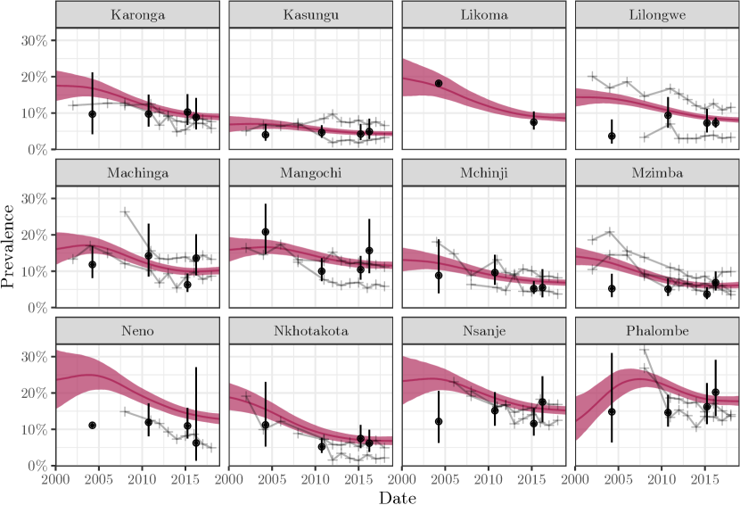
Figure 4: Data and estimates in 12 districts of Malawi. Circular points and line ranges represent point estimates and 95-percent confidence intervals from surveys. Connected series of crosses in the prevalence plot represent observed prevalence series from sentinel surveillance ANC clinics. Each red line is the median estimate for the corresponding metric, and each red region is corresponding 95-percent uncertainty interval.

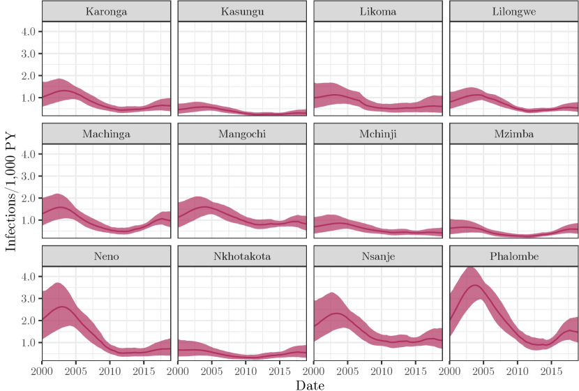
Figure 5: Data and estimates in 12 districts of Malawi. Each red line is the median estimate for the corresponding metric, and each red region is corresponding 95-percent uncertainty interval.

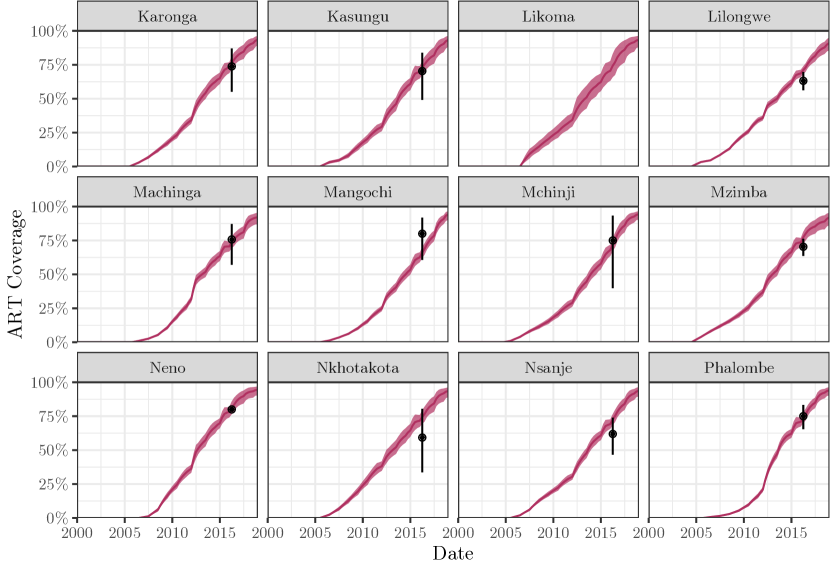
Figure 6: Data and estimates in 12 districts of Malawi. Circular points and line ranges represent point estimates and 95-percent confidence intervals from surveys. Each red line is the median estimate for the corresponding metric, and each red region is corresponding 95-percent uncertainty interval.

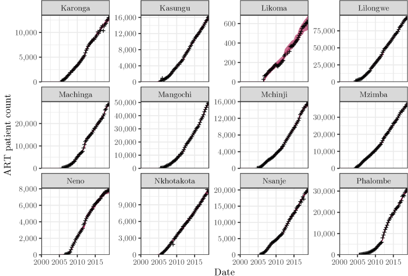
Figure 7: Data and estimates in 12 districts of Malawi. Non-connected crosses in the ART patient count plot represent reported programmatic patient counts. Each red line is the median estimate for the corresponding metric, and each red region is corresponding 95-percent uncertainty interval.

Figure 4 shows that the model seems to capture variation in HIV prevalence over space, time, and their interaction reasonably well. We are over estimating prevalence across the board in Neno, but the survey estimates there are so uncertain that we cannot include them on the plot. Interestingly, we predict that the epidemic peaked significantly later in Phalombe than in other districts. We also note that the model fit well to data from Likoma, for which we have far less data than for any other district.

In Figure 5, we see that our inferred incidence series also exhibit considerable heterogeneity over space and time. For example, the late prevalence peak we observed in Phalombe is reflected in a later, higher peak incidence. This figure also illustrates the value of fitting to multiple regions at once: we would never be able to produce incidence estimates in Likoma if we did not share information across regions.

Taking Figures 6 and 7 as a pair, we see that our model of ART initiation both produces plausible time series of both ART coverage and ART patient counts. We recognize that this is a particularly easy (exceptionally linear) case, but we believe that the results are still encouraging. Further work is required to thoroughly interrogate the model of ART initiation, but valid inference of the spatio-temporal variation in ART initiation could be a significant aid to policymakers. Figure 8 shows these estimates for the current set of results from the beginning of 2015 to the end of the study period. We can see that, even in the most recent timepoint, there is considerable heterogeneity.

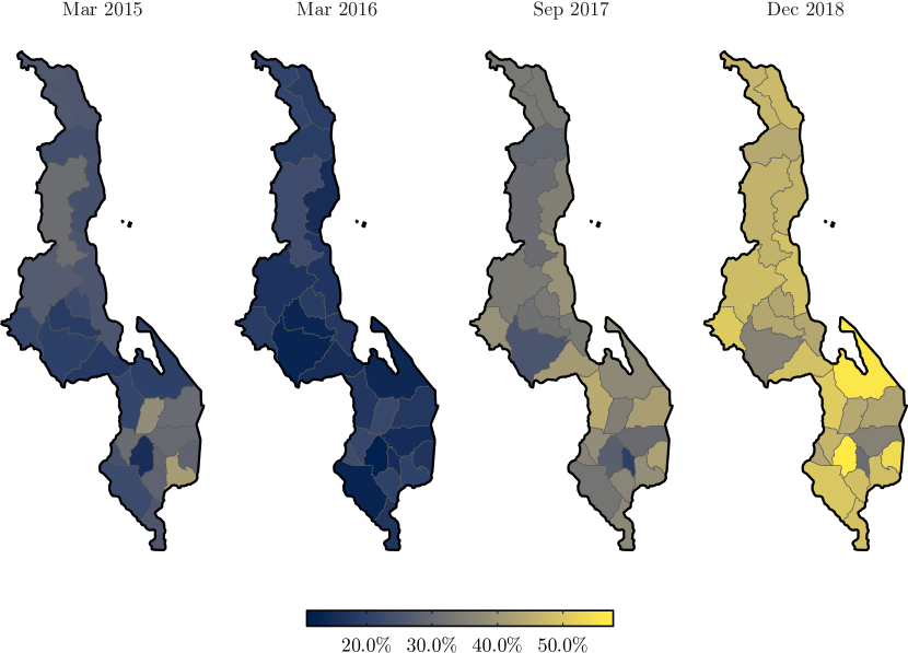
Figure 8: Inferred median ART initiation probabilities in Malawi, 2015-2018.

Our model of cross-region treatment seeking is also difficult to validate but seems to be performing well. Figure 9 shows the probability a person receiving ART in Dedza will seek treatment each of the districts that are within two degrees of adjacency from Dedza. The majority of treatment-seekers in Dedza stayed in their home region, but a significant portion went to Lilongwe, which contains the capital and largest city. Without allowing for cross-region treatment seeking, our model consistently overestimates prevalence in districts like Lilongwe and Chiradzulu, which have a longer history of high-quality treatment provision.

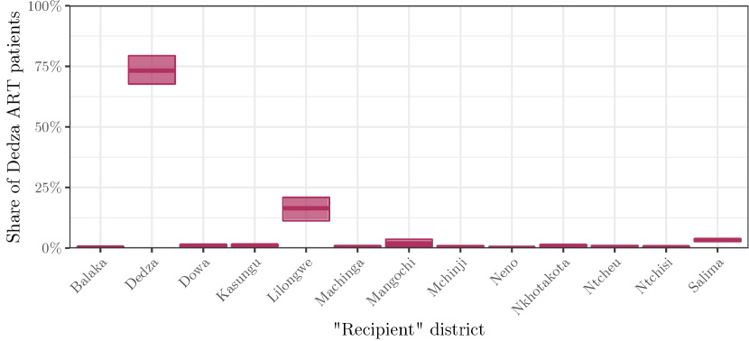
Figure 9: Estimated geographic distribution of treatment seeking among PLHIV residing in Dedza (median shares and 95-percent uncertainty intervals).

Most importantly, the model fits well to each of the data sources we provide to it. By adding flexibility in the models of HIV transmission rates and ART initiation probabilities, we can fit simultaneously to both traditional (seroprevalence measurements) and non-traditional (programmatic counts) data sources.

Conclusion

In this study, we present a multivariate model of population-level HIV that combines all available population-level data sources and exploits the spatial structure of existing data in order to facilitate more credible inference of HIV incidence at relatively granular geographic resolutions. Incidentally, the supporting spatio-temporal models of HIV transmission rates, ART initiation rates, and cross-region treatment seeking provide estimates of politically relevant indicators that cannot be obtained from the other models widely in use.

We believe that our work illustrates several key points:

1. Compartmental models of infectious disease are compatible with modern inferential frameworks. Using sparse matrices, we were able to cut down the cost of integrating our model to the point where, even at relatively large geographic scales, we can run the inference procedure on a laptop. We suspect that further computational gains could be found by performing calculations in parallel or on a graphics processing unit.

2. Accounting for the inherent spatial dynamics of HIV is critical at granular geographic resolutions. We observed considerable spatio-temporal heterogeneity in incidence, transmission, ART initiation, and cross-region treatment seeking. Neglecting to account for any of these spatial dynamics would hamper our inference of the others. In particular, models that did not allow individuals to seek treatment outside of their home region severely overestimated prevalence (and, hence, incidence) in many regions. By letting the model “reallocate” patients to nearby districts, we allow it to explain high ART patient counts without increasing prevalence to implausibly high levels.

3. The combined set of data sources is more valuable than the sum of its parts. Our compartmental model is an explicit link between each of the various observable indicators, so every indicator informs our estimates of every other indicator. For example, a proposed parameter set that predicts very high HIV prevalence would result in poor fit to not only the direct observation of prevalence, but also to ART coverage and ART patient counts.

4. Simultaneous modeling of multiple spatial units provides better inference in all cases. First, shrinkage priors allow us to estimate the initial state of the epidemic across regions even if some of those regions are data-sparse. Additionally, giving the model the flexibility to explain observations in one area with epidemic patterns in another area helps avoid implausible estimates. For example, sustained high prevalence in one area might be the result of poor treatment coverage in a nearby area.

Future Work

We are actively working on this model and foresee several improvements.

1. Greater demographic detail: Incorporating age and sex dynamics will allow us to build a more realistic model of mortality and population.

2. Incorporating population data: The model currently includes a demographic projection, but we neither fit to nor match any data on population levels. We plan to explore a strategy where the total population in each time is fixed (from exogenous estimation processes) and migration is calculated as the difference between modeled population and observed population. Alternatively, we could attempt to fit to census data, but we suspect that that is out of scope for this particular project.

3. Designing cross-validation scheme: We are currently fitting to all available data, but we would like to devise a cross-validation scheme that prioritizes validity in more recent years. The challenge is that we have relatively little data to begin with.

4. Tools for model comparison: Because this model is complex and nonlinear, we do not have access to the typical set of model comparison tools we would use in a regression setting. Finding the appropriate metrics to assess the effects of changes to both the structure of the model and the inferential procedure will be an important step in interrogating our results.

Acknowledgements

We are enormously grateful to our collaborators at the Department of HIV & AIDS in the Malawi Ministry of Health for their guidance and for providing access to these data. We also thank the Imperial DIDE HIV Inference Research Group for their helpful feedback.

Timothy M Wolock’s work is funded through the Imperial President’s PhD Scholarship.

References

Bao, Le. 2012. “A New Infectious Disease Model for Estimating and Projecting HIV/AIDS Epidemics.” Sexually Transmitted Infections 88 (Suppl_2): i58–i64. https://doi.org/10.1136/sextrans-2012-050689.

Brown, Tim, Le Bao, Jeffrey W. Eaton, Daniel R. Hogan, Mary Mahy, Kimberly Marsh, Bradley M. Mathers, and Robert Puckett. 2014. “Improvements in Prevalence Trend Fitting and Incidence Estimation in EPP 2013.” AIDS 28 (November): S415. https://doi.org/10.1097/QAD.0000000000000454.

Carpenter, Bob, Andrew Gelman, Matthew D. Hoffman, Daniel Lee, Ben Goodrich, Michael Betancourt, Marcus Brubaker, Jiqiang Guo, Peter Li, and Allen Riddell. 2017. “Stan: A Probabilistic Programming Language.” Journal of Statistical Software 76 (1): 1–32. https://doi.org/10.18637/jss.v076.i01.

Cuadros, Diego F., Jingjing Li, Adam J. Branscum, Adam Akullian, Peng Jia, Elizabeth N. Mziray, and Frank Tanser. 2017. “Mapping the Spatial Variability of HIV Infection in Sub-Saharan Africa: Effective Information for Localized HIV Prevention and Control.” Scientific Reports 7 (1): 9093. https://doi.org/10.1038/s41598-017-09464-y.

Dwyer-Lindgren, Laura, Michael A. Cork, Amber Sligar, Krista M. Steuben, Kate F. Wilson, Naomi R. Provost, Benjamin K. Mayala, et al. 2019. “Mapping HIV Prevalence in Sub-Saharan Africa Between 2000 and 2017.” Nature, May, 1. https://doi.org/10.1038/s41586-019-1200-9.

Fonner, Virginia A., Sarah L. Dalglish, Caitlin E. Kennedy, Rachel Baggaley, Kevin R. O’Reilly, Florence M. Koechlin, Michelle Rodolph, Ioannis Hodges-Mameletzis, and Robert M. Grant. 2016. “Effectiveness and Safety of Oral HIV Preexposure Prophylaxis for All Populations.” AIDS (London, England) 30 (12): 1973–83. https://doi.org/10.1097/QAD.0000000000001145.

Guennebaud, Gaël, Benoı^t Jacob, and others. 2010. Eigen V3. http://eigen.tuxfamily.org.

Gupta, Ravindra K., Sultan Abdul-Jawad, Laura E. McCoy, Hoi Ping Mok, Dimitra Peppa, Maria Salgado, Javier Martinez-Picado, et al. 2019. “HIV-1 Remission Following CCR5Delta32/Delta32 Haematopoietic Stem-Cell Transplantation.” Nature 568 (7751): 244–48. https://doi.org/10.1038/s41586-019-1027-4.

Gutreuter, Steve, Ehimario Igumbor, Njeri Wabiri, Mitesh Desai, and Lizette Durand. 2019. “Improving Estimates of District HIV Prevalence and Burden in South Africa Using Small Area Estimation Techniques.” PLOS ONE 14 (2): e0212445. https://doi.org/10.1371/journal.pone.0212445.

Hall, D.L., and J. Llinas. 1997. “An Introduction to Multisensor Data Fusion.” Proceedings of the IEEE 85 (1): 6–23. https://doi.org/10.1109/5.554205.

“HIV and AIDS in eSwatini. AVERT.” 2015. July 21, 2015. https://www.avert.org/professionals/hiv-around-world/sub-saharan-africa/swaziland.

Hütter, Gero, Daniel Nowak, Maximilian Mossner, Susanne Ganepola, Arne Müßig, Kristina Allers, Thomas Schneider, et al. 2009. “Long-Term Control of HIV by CCR5 Delta32/Delta32 Stem-Cell Transplantation.” New England Journal of Medicine 360 (7): 692–98. https://doi.org/10.1056/NEJMoa0802905.

ICAP at Columbia University, and PEPFAR. 2019. “Methodology. PHIA.” 2019. https://phia.icap.columbia.edu/methodology/.

Johnson, Leigh, and Rob Dorrington. 2019. Thembisa Version 4.2: A Model for Evaluating the Impact of HIV/AIDS in South Africa. https://www.thembisa.org/content/downloadPage/Thembisa4_2report.

Kassanjee, Reshma, Thomas A. McWalter, and Alex Welte. 2014. “Short Communication: Defining Optimality of a Test for Recent Infection for HIV Incidence Surveillance.” AIDS Research and Human Retroviruses 30 (1): 45–49. https://doi.org/10.1089/aid.2013.0113.

Kristensen, Kasper, Anders Nielsen, Casper W. Berg, Hans Skaug, and Brad Bell. 2016. “TMB: Automatic Differentiation and Laplace Approximation.” Journal of Statistical Software 70 (5). https://doi.org/10.18637/jss.v070.i05.

Lindén, Andreas, and Samu Mäntyniemi. 2011. “Using the Negative Binomial Distribution to Model Overdispersion in Ecological Count Data.” Ecology 92 (7): 1414–21. https://doi.org/10.1890/10-1831.1.

Marston, Milly, Jim Todd, Judith R. Glynn, Kenrad E. Nelson, Ram Rangsin, Tom Lutalo, Mark Urassa, et al. 2007. “Estimating ‘Net’ HIV-Related Mortality and the Importance of Background Mortality Rates.” AIDS (London, England) 21 (Suppl 6): S65–S71. https://doi.org/10.1097/01.aids.0000299412.82893.62.

Meyer-Rath, Gesine, Jessica B. McGillen, Diego F. Cuadros, Timothy B. Hallett, Samir Bhatt, Njeri Wabiri, Frank Tanser, and Thomas Rehle. 2018. “Targeting the Right Interventions to the Right People and Places: The Role of Geospatial Analysis in HIV Program Planning.” AIDS (London, England) 32 (8): 957–63. https://doi.org/10.1097/QAD.0000000000001792.

“Monitoring, Evaluation, and Reporting (MER 2.0) Indicator Reference Guide.” 2017. PEPFAR. https://www.pepfar.gov/documents/organization/263233.pdf.

Monnahan, Cole C., and Kasper Kristensen. 2018. “No-U-Turn Sampling for Fast Bayesian Inference in ADMB and TMB: Introducing the Adnuts and Tmbstan R Packages.” PLoS ONE 13 (5). https://doi.org/10.1371/journal.pone.0197954.

Sharp, Paul M., and Beatrice H. Hahn. 2011. “Origins of HIV and the AIDS Pandemic.” Cold Spring Harbor Perspectives in Medicine: 1 (1). https://doi.org/10.1101/cshperspect.a006841.

Skaug, Hans J., and David A. Fournier. 2006. “Automatic Approximation of the Marginal Likelihood in Non-Gaussian Hierarchical Models.” Computational Statistics & Data Analysis 51 (2): 699–709. https://doi.org/10.1016/j.csda.2006.03.005.

Stover, John, Tim Brown, Robert Puckett, and Wiwat Peerapatanapokin. 2017. “Updates to the Spectrum/Estimations and Projections Package Model for Estimating Trends and Current Values for Key HIV Indicators.” AIDS 31 (April): S5. https://doi.org/10.1097/QAD.0000000000001322.

“The DHS Program - DHS Methodology.” n.d. Accessed June 3, 2019. https://dhsprogram.com/What-We-Do/Survey-Types/DHS-Methodology.cfm.

Todd, Jim, Judith R. Glynn, Milly Marston, Tom Lutalo, Sam Biraro, Wambura Mwita, Vinai Suriyanon, et al. 2007. “Time from HIV Seroconversion to Death: A Collaborative Analysis of Eight Studies in Six Low and Middle-Income Countries Before Highly Active Antiretroviral Therapy.” AIDS (London, England) 21 (Suppl 6): S55–S63. https://doi.org/10.1097/01.aids.0000299411.75269.e8.

Yiannoutsos, Constantin Theodore, Leigh Francis Johnson, Andrew Boulle, Beverly Sue Musick, Thomas Gsponer, Eric Balestre, Matthew Law, Bryan E Shepherd, and Matthias Egger. 2012. “Estimated Mortality of Adult HIV-Infected Patients Starting Treatment with Combination Antiretroviral Therapy.” Sexually Transmitted Infections 88 (Suppl_2): i33–i43. https://doi.org/10.1136/sextrans-2012-050658.