Higher-order total variation approaches and generalisations

Abstract

Over the last decades, the total variation (TV) evolved to one of the most broadly-used regularisation functionals for inverse problems, in particular for imaging applications. When first introduced as a regulariser, higher-order generalisations of TV were soon proposed and studied with increasing interest, which led to a variety of different approaches being available today. We review several of these approaches, discussing aspects ranging from functional-analytic foundations to regularisation theory for linear inverse problems in Banach space, and provide a unified framework concerning well-posedness and convergence for vanishing noise level for respective Tikhonov regularisation. This includes general higher orders of TV, additive and infimal-convolution multi-order total variation, total generalised variation (TGV), and beyond. Further, numerical optimisation algorithms are developed and discussed that are suitable for solving the Tikhonov minimisation problem for all presented models. Focus is laid in particular on covering the whole pipeline starting at the discretisation of the problem and ending at concrete, implementable iterative procedures. A major part of this review is finally concerned with presenting examples and applications where higher-order TV approaches turned out to be beneficial. These applications range from classical inverse problems in imaging such as denoising, deconvolution, compressed sensing, optical-flow estimation and decompression, to image reconstruction in medical imaging and beyond, including magnetic resonance imaging (MRI), computed tomography (CT), magnetic-resonance positron emission tomography (MR-PET), and electron tomography.

AMSa”78

• November 2019

Contents

toc

1 Introduction

In this paper we give a review of higher-order regularisation functionals of total-variation type, encompassing their development from their origins to generalisations and most recent approaches. Research in this field has in particular been triggered by the success of the total variation (TV) as a regularisation functional for inverse problems on the one hand, but on the other hand by the insight that tailored regularisation approaches are indispensable for solving ill-posed inverse problems in theory and in practice. The last decades comprised active development of the latter topic which resulted in a variety of different strategies for TV-based regularisation functionals that model data with some inherent smoothness, possibly of higher order or multiple orders. For these functionals, this paper especially aims at providing a unified presentation of the underlying regularisation aspects, giving an overview of numerical algorithms suitable to solve associated regularised inverse problems as well as showing the breadth of respective applications.

Let us put classical and higher-order total-variation regularisation into an inverse problems context. From the inverse problems point of view, the central theme of regularisation is the stabilisation of the inversion of an ill-posed operator equation, which is commonly phrased as finding a $u\in X$ such that

$$K(u)=f$$

for given $K:X\to Y$ and $f\in Y$, where $X$ and $Y$ are usually Banach spaces. Various approaches for regularisation exist, e.g., iterative regularisation, Tikhonov regularisation, regularisation based on spectral theory in Hilbert spaces, or regularisation by discretization. Being a regularisation and providing a stable inversion is mathematically well-formalised [83], and usually comprises regularisation parameters. Essentially, stable inversion means that each regularised inverse mapping from data to solution space is continuous in some topology, and being a regularisation requires in addition that, in case the measured data approximates the noiseless situation, a suitable choice of the regularisation parameters allows to approximate a solution that is meaningful and matches the noiseless data. These properties are typically referred to as stability and convergence for vanishing noise, respectively. For general non-linear inverse problems, they usually depend on an interplay between the selected regularisation strategy and the forward operator $K$, where often, derivative-based assumptions on the local behaviour around the sought solution are made [83, 112]. In contrast, for linear forward operators, unified statements are commonly available such that regularisation properties solely depend on the regularisation strategy. We therefore consider linear inverse problems throughout the paper, i.e., the solution of $Ku=f$ where $K:X\to Y$ is always assumed to be linear and continuous.

Variational regularisation, which is the stabilised solution of such an inverse problems via energy minimisation methods, then encompasses — and is often identified with — Tikhonov regularisation (but comprises, for instance, also Morozov regularisation [135] or Ivanov regularisation [113]). Driven by its success in practical applications, it has become a major direction of research in inverse problems. Part of its success may be explained by the fact that variational regularisation allows to incorporate a modelling of expected solutions via regularisation functionals. In a Tikhonov framework, this means that the solution of the operator equation $Ku=f$ is obtained via solving

$$\min_{u\in X}\ S_{f}(Ku)+\mathcal{R}_{\alpha}(u),$$

where $S_{f}:Y\rightarrow[0,\infty]$ is an energy that measures the discrepancy between $Ku$ and the measured data $f$, and $\mathcal{R}_{\alpha}:X\rightarrow[0,\infty]$ is the regularisation functional that depends on regularisation parameters $\alpha$. From the analytical perspective, two main features of $\mathcal{R}_{\alpha}$ are important: First, it needs to possess properties that allow to guarantee that the corresponding solution map enjoys the stability and convergence properties as mentioned above (typically, lower semi-continuity and coercivity in some topology). Second, it needs to provide a good model of reasonable/expected solutions of $Ku=f$ in the sense that $\mathcal{R}_{\alpha}(u)$ is small for such reasonable solutions and $\mathcal{R}_{\alpha}(u)$ is large for unreasonable solutions that suffer, for instance, from artefacts or noise.

While the first requirement is purely qualitative and known to be true for a wide range of norms and seminorms, the second requirement involves the modelling of expected solutions as well as suitable quantification, having in particular in mind that the outcome should be simple enough to be amenable to numerical solution algorithms. Suitable models are for instance provided by various classical smoothness measures such as Hilbert scales of smooth functions, i.e., by $H^{s}$-norms where $s\geq 0$, but also reflexive Banach-space norms such as $L^{p}$-norms, associated Sobolev-space seminorms in $H^{k,p}$ for $1<p<\infty$, and Besov-space seminorms based on wavelet-coefficient expansions [169, 39, 68]. The reflexivity of the underlying spaces then helps to turn an ill-posed equation into a well-posed one, since the direct method in the calculus of variations can be employed with weak convergence.

However, there are reasons to consider Banach spaces that lack reflexivity, with $L^{1}$-spaces and spaces of Radon measures being prominent examples. Indeed, $L^{1}$-type norms as penalties in variational energies have seen a tremendous rise in popularity in the past two decades, most notably in the theory of compressed sensing [76]. This is due to their property of favouring sparsity in solutions, which allows to model more specific a-priori assumptions on the expected solutions than generic smoothness, for instance. While sparsity in $L^{1}$-type spaces over discrete domains, such as spaces of wavelet coefficients, is directly amenable to analysis, sparsity for continuous domains requires to consider spaces of Radon measures and corresponding Radon-norm-type energies which are natural generalisations of $L^{1}$-type norms. Being the dual of a separable normed space then mitigates the non-reflexivity of these spaces. As a consequence, they play a major role in continuous models for sparsity-promoting variational regularisation strategies.

A particular example is the total variation functional [161, 58], see Section 2 below for a precise definition, which can be interpreted as the Radon norm realised as a dual norm on the distributional derivative of $u$. As such, $\mathop{\rm TV}\nolimits(u)$ is finite if and only if the distributional derivative of $u$ can be represented by a finite Radon measure. The TV functional then penalises variations of $u$ via a norm on its derivative while still being finite in the case of jump discontinuities, i.e., when $u$ is piecewise smooth. In particular, its minimisation realises sparsity of the derivative which is often considered a suitable model for piecewise constant functions. In addition, it is convex and lower semi-continuous with respect to $L^{p}$-convergence for any $p\in[1,\infty]$, and coercive up to constants in suitable $L^{p}$-norm topologies. These features make TV a reasonable model for piecewise constant solutions and allow to obtain well-posedness of TV regularisation for a broad class of inverse problems. They can be considered as some of the main reasons for the overwhelming popularity of TV in inverse problems, imaging sciences and beyond.

Naturally, the simplicity and desirable properties of TV come with a cost. As previously mentioned, interpreting TV as a functional that generalises the $L^{1}$-norm of the image gradient, compressed sensing theory suggests that this enforces sparsity of the gradient and hence piecewise constancy, i.e., one might expect that a TV-regularised function is non-constant only on low-dimensional subsets of its domain. While this might in fact be a feature if the sought solution is piecewise constant, it is not appropriate for general piecewise smooth data. Indeed, for non-piecewise-constant data, TV has the defect of producing artificial plateau-like structures in the reconstructions which became known as the staircasing effect of TV. This effect is nowadays well-understood analytically in the case of denoising [138, 54, 157], and recent results also provide an analytical confirmation of this fact in the context of inverse problems with finite-dimensional measurement data [29, 26]. The appearance of staircasing artefacts is in particular problematic since jump discontinuities are features which are, on the one hand, very prominent in visual perception and typically associated with relevant structures, and, on the other hand, important for automatic post-processing or interpretation of the data. As a result, it became an important research question in the past two decades how to improve upon this defect of TV regularisation while maintaining its desirable features, especially the sparsity-enforcing properties.

This review is concerned with the developments undertaken in this direction that are related to the incorporation of higher-order derivatives, while maintaining the sparsity concepts realised by the Radon norm and the underlying spaces of Radon measures. This resulted in a variety of different variational regularisation strategies, for which some are very successful in achieving the goal of providing an amenable model for piecewise smooth solutions. It is also a central message of this review that the success of higher-order TV model in terms of modelling and regularisation effect depends very much on the structure and the functional-analytic setting in which the higher-order derivatives are included. Following this insight, we will discuss different higher-order regularisation functionals such as higher-order total variation, the infimal-convolution of higher-order TV as well as the total generalised variation (TGV), which carries out a cascadic decomposition to different orders of differentiation. Starting form the analytical framework of the total-variation functional and functions of bounded variation, we will introduce and analyse several higher-order approaches in a continuous setting, discuss their regularisation properties in a Tikhonov regularisation framework, introduce appropriate discretizations as well as numerical solution strategies for the resulting energy minimisation problems, and present various applications in image processing, computer vision, biomedical imaging and beyond.

Nevertheless, due to the broad range of the topic as well as the many works published in its environment, it is impossible to give a complete overview. The various references to the literature given throughout the paper therefore only represent a selection. Let us also point out that we selected the presented material in particular on a basis that, one the one hand, enables a treatment that is a unified as possible. On the other hand, a clear focus is put on approaches for which the whole pipeline ranging from mathematical modelling, embedding into a functional-analytic context, proof of regularisation properties, numerical discretization, optimisation algorithms and efficient implementation can be covered. In addition, extensions and further developments will shortly be pointed out when appropriate. Especially, many of the applications in image processing, computer vision, medical imaging and image reconstruction refer to these extensions. The applications were further chosen to represent a wide spectrum of inverse problems, their variational modelling and higher-order TV-type regularisation, and, not negligible, successful realisation of the presented theory. We finally aimed at providing a maximal amount of useful information regarding theory and practical realisation in this context.

2 Total-variation (TV) regularisation

Before discussing higher-order total variation and how it may be used to regularise ill-posed inverse problems, let us begin with an overview of first-order total variation. Throughout the review, we mainly adapt a continuous viewpoint which means that the objects of interest are usually functions on some fixed domain $\Omega$, i.e., an non-empty, open and connected subset $\Omega\subset\mathbf{R}^{d}$ in the $d$-dimensional Euclidean space. This requires in particular a common functional-analytic context for which we assume that the reader is familiar with and refer to the books [1, 84, 202] for further information. In the following, we will make, for instance, use of the Lebesgue spaces $L^{p}({\Omega,H})$ for $H$-valued functions where $H$ is a finite-dimensional real Hilbert space as well as their measure-theoretic and functional-analytic properties. Also, concepts of weak differentiability and properties of the associated Sobolev spaces $H^{k,{p}}(\Omega,H)$ will be utilised without further introduction. This moreover applies to the classical spaces such as $\mathcal{C}({\overline{\Omega},H})$, $\mathcal{C}_{\mathrm{c}}({\Omega,H})$ and $\mathcal{C}_{0}({\Omega,H})$, i.e., the spaces of uniformly continuous functions on $\overline{\Omega}$, of compactly supported continuous functions on $\Omega$ and its closure with respect to the supremum norm. As usual, the respective spaces of $k$-times continuously differentiable functions are denoted by $\mathcal{C}^{k}({\overline{\Omega},H})$, $\mathcal{C}_{\mathrm{c}}^{k}({\Omega,H})$ and $\mathcal{C}_{0}^{k}({\Omega,H})$ where $k$ could also be infinity, leading to spaces of test functions.

We further employ, throughout this section, basic concepts from convex analysis and optimisation. At this point, we would like to recall that for a convex function $F:X\to{]{-\infty,\infty}]}$ defined on a Banach space $X$, the subgradient $\partial F(x)$ at a point $u\in X$ is the collection of all $w\in X^{*}$ that satisfy the subgradient inequality

$$F(u)+\langle{w},\,{v-u}\rangle_{X^{*}\times X}\leq F(v)\qquad\mbox{for all}\quad v\in X.$$

For $F$ proper, the Fenchel dual or Fenchel conjugate of $F$ is the function $F^{*}:X^{*}\to{]{-\infty,\infty}]}$ defined by

$$F^{*}(w)=\sup_{u\in X}\ \langle{w},\,{u}\rangle_{X^{*}\times X}-F(u).$$

The Fenchel inequality then states that $\langle{w},\,{u}\rangle_{X^{*}\times X}\leq F(u)+F^{*}(w)$ for all $u\in X$ and $w\in X^{*}$ with equality if and only if $w\in\partial F(u)$. For more details regarding these notions and convex analysis in general, we refer to research monographs covering this subject, for instance [82, 196].

2.1 Functions of bounded variation

Generally, when solving a specific ill-posed inverse problem with, for instance, Tikhonov regularisation, one usually has many choices regarding the regularisation functional. Now, while functionals associated with Hilbertian norms or seminorms possess several advantages such as smoothness and allow, in addition, for regularisation strategies that can be computed by solving a linear equation, they are often not able to provide a good model for piecewise smooth functions. This can, for instance, be illustrated as follows.

Example 2.1.

Classical Sobolev spaces cannot contain non-trivial piecewise constant functions. Let $\Omega\subset\mathbf{R}^{d}$ be a domain and $\Omega^{\prime}\subset\Omega$ be non-empty, open with $\partial\Omega^{\prime}$ a null set. Then, the characteristic function $u=\chi_{\Omega^{\prime}}$, i.e., $u(x)=1$ if $x\in\Omega^{\prime}$ and $0$ otherwise, is not contained in $H^{1,{p}}(\Omega)$ for any $p\in[1,\infty]$. To see this, suppose that $v\in L^{p}({\Omega,\mathbf{R}^{d}})$ is the weak derivative of $u$. Let $\varphi\in\mathcal{C}_{\mathrm{c}}^{\infty}({\Omega^{\prime}})$ be a test function. Clearly,

$$\int_{\Omega}v\cdot\varphi\ \mathrm{d}{x}=-\int_{\Omega}u\mathop{\rm div}\nolimits\varphi\ \mathrm{d}{x}=-\int_{\Omega^{\prime}}\mathop{\rm div}\nolimits\varphi\ \mathrm{d}{x}=0.$$

Hence, $v=0$ on $\Omega^{\prime}$. Likewise, one sees that also $v=0$ on $\Omega\backslash\overline{\Omega^{\prime}}$. In total, $v=0$ almost everywhere and as $v$ is the weak derivative of $u$, $u$ must be constant which is a contradiction.

The defect which is responsible for the failure of characteristic function being (classical) Sobolev function can, however, be remedied by allowing weak derivatives to be Radon measures. These are in particular able to concentrate on Lebesgue null-sets; a property that is necessary as the previous example just showed. In the following, we introduce some basic notions and results about vector-valued Radon measures, in particular, with an eye of embedding them into a functional-analytic framework. Moreover, we would like to have these notions readily available when dealing with higher-order derivatives and the associated higher-order total variation.

Throughout this section, let $\Omega\subset\mathbf{R}^{d}$ be a domain and $H$ a non-trivial finite-dimensional real Hilbert space with $\cdot$ and ${|{\,\cdot\,}|}$ denoting the associated scalar product and norm, respectively. As usual, the case $H=\mathbf{R}$ corresponds to the scalar case and $H=\mathbf{R}^{d}$ to the vector-field case, but, as we will see later, $H$ could also be a space of higher-order tensors. The following definitions and statements regarding basic measure theory and can, for instance, be found in [7].

Definition 2.2.

A vector-valued Radon measure or $H$-valued Radon measure on $\Omega$ is a function $\mu:\mathcal{B}({\Omega})\to H$ on the Borel $\sigma$-algebra $\mathcal{B}({\Omega})$ associated with the standard topology on $\Omega$ satisfying the following properties:

1. It holds that $\mu(\emptyset)=0$,

2. for each pairwise disjoint countable collection $A_{1},A_{2},\ldots$ in $\mathcal{B}({\Omega})$ it holds that $\mu(\bigcup_{i\in\mathbf{N}}A_{i})=\sum_{i=1}^{\infty}\mu(A_{i})$ in $H$.

A positive Radon measure is a function $\mu:\mathcal{B}({\Omega})\to[0,\infty]$ satisfying (1), (2) (with $H$ replaced by $[0,\infty]$) as well as $\mu(K)<\infty$ for each compact $K\subset\subset\Omega$. It is called finite, if $\mu(\Omega)<\infty$.

Naturally, vector-valued Radon measures can be associated to an integral. For $\mu$ an $H$-valued Radon measure and step functions $u=\sum_{j=1}^{N}c_{j}\chi_{A_{j}}$, $v=\sum_{j=1}^{N}v_{j}\chi_{A_{j}}$ with $c_{1},\ldots,c_{N}\in\mathbf{R}$, $v_{1},\ldots,v_{N}\in H$ and $A_{1},\ldots,A_{N}\in\mathcal{B}({\Omega})$, the following integrals make sense:

$$\int_{\Omega}u\ \mathrm{d}{\mu}=\sum_{j=1}^{N}c_{j}\mu(A_{j})\in H,\qquad\int_{\Omega}v\cdot\ \mathrm{d}{\mu}=\sum_{j=1}^{N}v_{j}\cdot\mu(A_{j})\in\mathbf{R}.$$

For uniformly continuous functions $u:\overline{\Omega}\to\mathbf{R}$ and $v:\overline{\Omega}\to H$, the integrals are given as

$$\int_{\Omega}u\ \mathrm{d}{\mu}=\lim_{n\to\infty}\int_{\Omega}u^{n}\ \mathrm{d}{\mu},\qquad\int_{\Omega}v\cdot\ \mathrm{d}{\mu}=\lim_{n\to\infty}\int_{\Omega}v^{n}\cdot\ \mathrm{d}{\mu}$$

where $\{{u^{n}}\}$ and $\{{v^{n}}\}$ are sequences of step functions converging uniformly to $u$ and $v$, respectively. Of course, the above integrals are well-defined, meaning that there are approximating sequences as stated and the above limits exist independently of the specific choice of the approximating sequences. The following definition is the basis for introducing a norm for $H$-valued Radon measures.

Definition 2.3.

For a vector-valued Radon measure $\mu$ on $\Omega$ the positive Radon measure ${|{\mu}|}$ given by

$${|{\mu}|}(A)=\sup\ \Bigl{\{}{\sum_{i=1}^{\infty}{|{\mu(A_{i})}|}}\ \Bigl{|}\ {A_{1},A_{2},\ldots\in\mathcal{B}({\Omega})\ \mbox{pairwise disjoint},\ A_{i}\subset A\ \mbox{for all}\ i\in\mathbf{N}}\Bigr{\}}$$

is called the total-variation measure of $\mu$.

The total-variation measure is always positive and finite, i.e., $0\leq{|{\mu}|}(A)<\infty$ for all $A\in\mathcal{B}({\Omega})$. By construction, $\mu$ is absolutely continuous with respect to ${|{\mu}|}$, i.e., $\mu(A)=0$ whenever ${|{\mu}|}(A)=0$ for a $A\in\mathcal{B}({\Omega})$. By Radon–Nikodým’s theorem, we thus have that each $H$-valued Radon measure $\mu$ can be written as $\mu=\sigma_{\mu}{|{\mu}|}$ with $\sigma_{\mu}\in L^{\infty}_{{|{\mu}|}}({\Omega,H})$ such that $\|{\sigma_{\mu}}\|_{\infty}\leq 1$ and ${|{\sigma_{\mu}}|}=1$ almost everywhere with respect to ${|{\mu}|}$. In this light, integration can also be phrased as

$$\int_{\Omega}u\ \mathrm{d}{\mu}=\int_{\Omega}u\sigma_{\mu}\ \mathrm{d}{{|{\mu}|}},\qquad\int_{\Omega}v\cdot\ \mathrm{d}{\mu}=\int_{\Omega}v\cdot\sigma_{\mu}\ \mathrm{d}{{|{\mu}|}}$$

for $u:\overline{\Omega}\to\mathbf{R}$, $v:\overline{\Omega}\to H$ uniformly continuous. The following theorem, which is a direct consequence of [162, Theorem 6.19], provides a useful characterisation of the space of vector valued measures as the dual of a separable space.

Proposition 2.4.

The space $\mathcal{M}({\Omega,H})$ of all vector-valued Radon measures equipped with the norm $\|{\mu}\|_{\mathcal{M}}={|{\mu}|}(\Omega)$ for $\mu\in\mathcal{M}({\Omega,H})$ is a Banach space.

It can be identified with the dual space $\mathcal{C}_{0}({\Omega,H})^{*}$ as follows. For each $T\in\mathcal{C}_{0}({\Omega,H})^{*}$ there exists a unique $\mu\in\mathcal{M}({\Omega,H})$ such that

$$\|{T}\|_{\mathcal{C}_{0}^{*}}=\|{\mu}\|_{\mathcal{M}},\qquad T(\varphi)=\int_{\Omega}\varphi\cdot\ \mathrm{d}{\mu}\quad\mbox{for all}\quad\varphi\in\mathcal{C}_{0}({\Omega,H}).$$

In particular, one has a notion of weak*-convergence of Radon measures. For a sequence $\{{\mu^{n}}\}$ and an element $\mu^{*}$ in $\mathcal{M}({\Omega,H})$ we have that $\mu^{n}\stackrel{{\scriptstyle*}}{{\rightharpoonup}}\mu^{*}$ in $\mathcal{M}({\Omega,H})$ if

$$\mbox{for all}\ \ \varphi\in\mathcal{C}_{0}({\Omega,H}):\quad\int_{\Omega}\varphi\cdot\ \mathrm{d}{\mu^{n}}\to\int_{\Omega}\varphi\cdot\ \mathrm{d}{\mu^{*}}\ \ \mbox{as}\ \ n\to\infty.$$

As the predual space $\mathcal{C}_{0}({\Omega,H})$ is separable, the Banach–Alaoglu theorem yields in particular the sequential relative weak*-compactness of bounded sets. That means for instance that a bounded sequence always admits a weakly*-convergent subsequence, a property that may compensate for the lack of reflexivity of $\mathcal{M}({\Omega,H})$.

The interpretation as a dual space as well as the density of test functions in $\mathcal{C}_{0}({\Omega,H})$ also allows to conclude that in order for a linear functional $T$ defining a Radon measure, it suffices to test against $\varphi\in\mathcal{C}_{\mathrm{c}}^{\infty}({\Omega,H})$ and to establish ${|{T(\varphi)}|}\leq C\|{\varphi}\|_{\infty}$ for all $\varphi\in\mathcal{C}_{\mathrm{c}}^{\infty}({\Omega,H})$ and $C>0$ independent of $\varphi$. This is useful for derivatives, i.e., the derivative of a $u\in L^{1}_{\mathrm{loc}}({\Omega,H})$ defines a Radon measure in $\mathcal{M}({\Omega,H^{d}})$ if

$$\Bigl{|}{\int_{\Omega}u\cdot\mathop{\rm div}\nolimits\varphi\ \mathrm{d}{x}}\Bigr{|}\leq C\|{\varphi}\|_{\infty}\qquad\mbox{for all}\quad\varphi\in\mathcal{C}_{\mathrm{c}}^{\infty}({\Omega,H^{d}}).$$ (1)

In this case, we denote by $\nabla u\in\mathcal{M}({\Omega,H^{d}})$ the unique $H^{d}$-valued Radon measure for which $\int_{\Omega}\varphi\cdot\ \mathrm{d}{\nabla u}=-\int_{\Omega}u\mathop{\rm div}\nolimits\varphi\ \mathrm{d}{x}$ for all $\varphi\in\mathcal{C}_{\mathrm{c}}^{\infty}({\Omega,H^{d}})$. Here, $H^{d}$ is equipped with the scalar product $x\cdot y=\sum_{i=1}^{d}x_{i}\cdot y_{i}$ for $x,y\in H^{d}$. In the case where (1) fails, there exists a sequence $\{{\varphi^{n}}\}$ in $\mathcal{C}_{\mathrm{c}}^{\infty}({\Omega,\mathbf{R}^{d}})$ with $\|{\varphi^{n}}\|_{\infty}=1$ and ${|{\int_{\Omega}u\cdot\mathop{\rm div}\nolimits\varphi\ \mathrm{d}{x}}|}\to\infty$ as $n\to\infty$. Thus, allowing the supremum to take the value $\infty$, this yields following definition.

Definition 2.5.

The total variation of a $u\in L^{1}_{\mathrm{loc}}({\Omega,H})$ is the value

$$\mathop{\rm TV}\nolimits(u)=\sup\ \Bigl{\{}{\int_{\Omega}u\cdot\mathop{\rm div}\nolimits\varphi\ \mathrm{d}{x}}\ \Bigl{|}\ {\varphi\in\mathcal{C}_{\mathrm{c}}^{\infty}({\Omega,H^{d}}),\ \|{\varphi}\|_{\infty}\leq 1}\Bigr{\}}.$$

Clearly, in case $\mathop{\rm TV}\nolimits(u)<\infty$, we have $\nabla u\in\mathcal{M}({\Omega,H^{d}})$ with $\|{\nabla u}\|_{\mathcal{M}}=\mathop{\rm TV}\nolimits(u)$. Trivially, for scalar functions, i.e., $H=\mathbf{R}$, one recovers the well-known definition [7, 161]. Also, one immediately sees that $\mathop{\rm TV}\nolimits$ is invariant to translations and rotations, or, more generally, to Euclidean-distance preserving transformations. This is the reason that this definition is also referred to as the isotropic total variation.

Example 2.6.

Piecewise constant functions may have a Radon measure as derivative. Let $\Omega^{\prime}\subset\Omega$ be a subdomain such that $\partial\Omega^{\prime}\cap\Omega$ can be parameterised by finitely many Lipschitz mappings. Then, the outer normal $\nu$ exists almost everywhere in $\partial\Omega^{\prime}\cap\Omega$ with respect to the Hausdorff $\mathcal{H}^{d-1}$ measure and one can employ the divergence theorem. This yields, for $u=\chi_{\Omega^{\prime}}$ and $\varphi\in\mathcal{C}_{\mathrm{c}}^{\infty}({\Omega,\mathbf{R}^{d}})$ with $\|{\varphi}\|_{\infty}\leq 1$ that

$$\int_{\Omega}u\mathop{\rm div}\nolimits\varphi\ \mathrm{d}{x}=\int_{\partial\Omega^{\prime}\cap\Omega}\varphi\cdot\nu\ \mathrm{d}{\mathcal{H}^{d-1}}=\int_{\Omega}\varphi\cdot\ \mathrm{d}{\nu\mathcal{H}^{d-1}\>\llcornernew\>(\partial\Omega^{\prime}\cap\Omega)}\leq\mathcal{H}^{d-1}(\partial\Omega^{\prime}\cap\Omega)$$

so $\nabla u=-\nu\mathcal{H}^{d-1}\>\llcornernew\>(\partial\Omega^{\prime}\cap\Omega)$ is a Radon measure. One sees, for instance via approximation, that $\|{\nabla u}\|_{\mathcal{M}}=\mathcal{H}^{d-1}(\partial\Omega^{\prime}\cap\Omega)$.

The class of sets $\Omega^{\prime}\subset\Omega$ for which $\chi_{\Omega^{\prime}}$ possesses a Radon measure as weak derivative is actually much greater than the class of bounded Lipschitz domains. These are the sets of finite perimeter, denoted by $\mathop{\rm Per}\nolimits(\Omega^{\prime})=\|{\nabla\chi_{\Omega^{\prime}}}\|_{\mathcal{M}}$. One the other hand, for $u\in H^{1,{1}}(\Omega)$, we have $\mathop{\rm TV}\nolimits(u)=\int_{\Omega}{|{\nabla u}|}\ \mathrm{d}{x}$ and the weak derivative as Radon measure is just $\nabla u\mathcal{L}^{d}$, i.e., the Sobolev derivative interpreted as a weight on the Lebesgue measure. Collecting all functions whose weak derivative is a Radon measure, we arrive at the following space.

Definition 2.7.

The space

$$\mathop{\rm BV}\nolimits(\Omega,H)=\{{u\in L^{1}({\Omega,H})}\ \bigl{|}\ {\mathop{\rm TV}\nolimits(u)<\infty}\},\qquad\|{u}\|_{\mathop{\rm BV}\nolimits}=\|{u}\|_{1}+\mathop{\rm TV}\nolimits(u)$$

is the space of $H$-valued functions of bounded variation. In case $H=\mathbf{R}$, we denote by $\mathop{\rm BV}\nolimits(\Omega)=\mathop{\rm BV}\nolimits(\Omega,\mathbf{R})$ and just refer to functions of bounded variation.

Proposition 2.8.

The space $\mathop{\rm BV}\nolimits(\Omega,H)$ with the associated norm is a Banach space. The total variation functional $\mathop{\rm TV}\nolimits$ is a continuous seminorm on $\mathop{\rm BV}\nolimits(\Omega,H)$ which vanishes exactly at the constant functions, i.e., $\ker(\mathop{\rm TV}\nolimits)=H\mathbf{1}$, with $H\mathbf{1}$ being the set of constant, $H$-valued functions.

The total variation functional is just designed to possess many convenient properties [7].

Proposition 2.9.

• The functional $\mathop{\rm TV}\nolimits$ is proper, convex and lower semi-continuous on each $L^{p}({\Omega,H})$, i.e., for $1\leq p\leq\infty$.

• For $1\leq p<\infty$, each $u\in\mathop{\rm BV}\nolimits(\Omega,H)\cap L^{p}({\Omega,H})$ can smoothly be approximated as follows: For $\varepsilon>0$, there exists $u^{\varepsilon}\in\mathcal{C}^{\infty}({\Omega,H})\cap\mathop{\rm BV}\nolimits(\Omega,H)\cap L^{p}({\Omega,H})$ such that

  $$\|{u-u^{\varepsilon}}\|_{p}\leq\varepsilon,\qquad{|{\mathop{\rm TV}\nolimits(u)-\mathop{\rm TV}\nolimits(u^{\varepsilon})}|}\leq\varepsilon.$$

• If $\Omega$ is a bounded Lipschitz domain, then there exists a constant $C>0$ such that for each $u\in\mathop{\rm BV}\nolimits(\Omega,H)$ with $\int_{\Omega}u\ \mathrm{d}{x}=0$, the Poincaré–Wirtinger estimate

  $$\|{u}\|_{d/(d-1)}\leq C\mathop{\rm TV}\nolimits(u)$$

  holds.

From the regularisation-theoretic point of view, the fact that $\mathop{\rm TV}\nolimits$ is proper, convex and lower semi-continuous on Lebesgue spaces is relevant, a property that fails for the Sobolev-seminorm $\|{\nabla\,\cdot\,}\|_{1}$. The Poincaré–Wirtinger estimate can be interpreted as a coercivity property on a subspace with codimension 1. Also note that this estimate is the same as for $H^{1,{1}}(\Omega,H)$-functions and the respective constants $C$ coincide. Consequently, the embedding properties of the latter space transfer immediately.

Proposition 2.10.

Let $\Omega$ is a bounded Lipschitz domain. Then,

• the embedding $\mathop{\rm BV}\nolimits(\Omega,H)\hookrightarrow L^{d/(d-1)}({\Omega,H})$ (with $d/(d-1)=\infty$ for $d=1$) exists and is continuous,

• the embedding $\mathop{\rm BV}\nolimits(\Omega,H)\hookrightarrow L^{p}({\Omega,H})$ is compact for each $1\leq p<d/(d-1)$,

• each bounded sequence $\{{u^{n}}\}$ in $\mathop{\rm BV}\nolimits(\Omega,H)$ possesses a subsequence $\{{u^{n_{k}}}\}$ which converges to a $u\in\mathop{\rm BV}\nolimits(\Omega,H)$ weak* in $\mathop{\rm BV}\nolimits(\Omega,H)$, which we define as $u^{n_{k}}\to u$ in $L^{1}({\Omega,H})$, $\nabla u^{n_{k}}\stackrel{{\scriptstyle*}}{{\rightharpoonup}}\nabla u$ in $\mathcal{M}({\Omega,H^{d}})$ as $k\to\infty$.

Consequently, the total variation is suitable for regularising ill-posed inverse problems in certain $L^{p}$-spaces.

2.2 Tikhonov regularisation

Let us now turn to solving ill-posed inverse problems with Tikhonov regularisation and $\mathop{\rm BV}\nolimits$-based penalty, i.e., solving

$$Ku=f$$

for some data $f$ in a Banach space $Y$. As mentioned in the introduction, since the focus of this review is on regularisation terms rather than tackling inverse problems in the most possible generality, we restrict ourselves here to linear and continuous forward operators $K:L^{d/(d-1)}({\Omega})\to Y$. Nevertheless we note that, building on the results developed here for the linear setting, an extension to non-linear operators typically boils down to ensuring additional requirements on the non-linear forward model rather than the regularisation term, see for instance [181, 83, 105].

Measuring the discrepancy in terms of the norm in $Y$, the problem is then to solve

$$\min_{u\in\mathop{\rm BV}\nolimits(\Omega)}\ \frac{\|{Ku-f}\|_{Y}^{q}}{q}+\alpha\int_{\Omega}\ \mathrm{d}{{|{\nabla u}|}}$$

for some exponent $q\geq 1$. Usually, $Y$ is some Hilbert space and $q=2$, resulting in a quadratic discrepancy, which is often used in case of Gaussian noise. For impulsive noise (or salt-and-pepper noise), the space $Y=L^{1}({\Omega^{\prime}})$, with $\Omega^{\prime}$ a domain, turns out to be useful. In case of Poisson noise, however, it is not advisable to take the norm but rather the Kullback–Leibler divergence between $Ku$ and $f$, i.e. $\mathop{\rm KL}\nolimits(Ku,f)$, where $\mathop{\rm KL}\nolimits$ is given, for $f\in L^{1}({\Omega^{\prime}})$ with $f\geq 0$ almost everywhere, according to the non-negative integral

$$\mathop{\rm KL}\nolimits(v,f)=\int_{\Omega^{\prime}}f\Bigl{(}\frac{v}{f}-\log\Bigl{(}\frac{v}{f}\Bigr{)}-1\Bigr{)}\ \mathrm{d}{x}$$ (2)

provided that $v\geq 0$ a.e., and $\infty$ else. In particular, in this context, we agree to set the integrand to $v$ where $f=0$ and to $\infty$ where $v=0$ and $f>0$.

In the following, we assume to have given a discrepancy functional $S_{f}:Y\to[0,\infty]$ that is proper, convex, lower semi-continuous and coercive. This is not the most general case but will be sufficient for us in order to ensure existence of minimizers of the Tikhonov functional.

Theorem 2.11.

Let $\Omega$ be a bounded Lipschitz domain, $Y$ be a Banach space, $K:L^{d/(d-1)}({\Omega})\to Y$ linear and continuous (weak*-to-weak-continuous in case $d=1$), $S_{f}:Y\to{[{0,\infty}]}$ a proper, convex, lower semi-continuous and coercive discrepancy functional associated with some data $f$ and $\alpha>0$. Then, there exist solutions of

$$\min_{u\in L^{d/(d-1)}({\Omega})}\ S_{f}(Ku)+\alpha\mathop{\rm TV}\nolimits(u).$$ (3)

If $S_{f}$ is strictly convex and $K$ is injective, the solution is unique whenever the minimum is finite.

We provide the proof for the sake of completeness and as a prototype for the generalisation to higher-order functionals.

Proof.

Assume that the objective functional in (3) is proper, otherwise, there is nothing to show. For a minimising sequence $\{{u^{n}}\}$, the Poincaré–Wirtinger inequality gives boundedness of $\{{u^{n}-{|{\Omega}|}^{-1}\int_{\Omega}u^{n}\ \mathrm{d}{x}}\}$ in $L^{d/(d-1)}({\Omega})$ while the coercivity of $S_{f}$ yields the boundedness of $\{{Ku^{n}}\}$. By continuity, $\{{K(u^{n}-{|{\Omega}|}^{-1}\int_{\Omega}u^{n}\ \mathrm{d}{x})}\}$ must be bounded, so if $K\mathbf{1}\neq 0$, then $\{{\int_{\Omega}u^{n}\ \mathrm{d}{x}}\}$ is bounded as otherwise, $\{{Ku^{n}}\}$ would be unbounded. In the case that $K\mathbf{1}=0$, we can without loss of generality assume that $\int_{\Omega}u^{n}\ \mathrm{d}{x}=0$ for all $n$ as shifting along constants does not change the functional value. In each case, $\{{\int_{\Omega}u^{n}\ \mathrm{d}{x}}\}$ is bounded, so $\{{u^{n}}\}$ must be bounded in $L^{d/(d-1)}({\Omega})$. Hence, by compact embedding (Proposition 2.10) we have $u^{n_{k}}\to u^{*}$ in $L^{1}({\Omega})$ as $k\to\infty$ for a subsequence $\{{u^{n_{k}}}\}$ and $u^{*}\in\mathop{\rm BV}\nolimits(\Omega)$. Reflexivity and continuity of $K$ (weak* sequential compactness and weak*-to-weak continuity in case $d=1$) give $Ku^{n_{k}}\rightharpoonup Ku^{*}$ in $Y$ for another subsequence (not relabelled). By lower semi-continuity, $u^{*}$ has to be a solution to (3).

Finally, if $S_{f}$ is strictly convex and $K$ is injective, then $S_{f}\circ K$ is already strictly convex, so minimizers have to be unique. ∎

Example 2.12.

• The discrepancy functional $S_{f}(v)=\frac{1}{q}\|{v-f}\|_{Y}^{q}$ for some $f\in Y$ is obviously proper, convex, lower semi-continuous and coercive.

• It follows from Lemma A.1 in the appendix that the discrepancy $S_{f}(v)=\mathop{\rm KL}\nolimits(v,f)$ defined on $Y=L^{1}({\Omega^{\prime}})$ for $f\in L^{1}({\Omega^{\prime}})$ with $f\geq 0$ almost everywhere is proper, convex and coercive in $L^{1}(\Omega^{\prime})$. Lower semi-continuity in turn follows as special case of Lemma A.2.

Remark 2.13.

Note that if the inversion of $K:L^{p}({\Omega})\to Y$ is well-posed for some $p\in[1,\infty]$, then solutions of (3) still exist (even for $\alpha=0$). Clearly, the $\mathop{\rm TV}\nolimits$ penalty is not necessary for obtaining a regularising effect for these problems. In this case, minimising the Tikhonov function with $\mathop{\rm TV}\nolimits$ penalty may the interpreted as denoising. The most prominent example might be the Rudin-Osher-Fatemi problem [161] which reads as

$$\min_{u\in L^{2}({\Omega})}\ \frac{1}{2}\int_{\Omega}{|{u-f}|}^{2}\ \mathrm{d}{x}+\alpha\mathop{\rm TV}\nolimits(u)$$

for $f\in L^{2}({\Omega})$. Here, as the identity is “inverted”, the effect of total-variation regularisation can be studied in detail. Minimisation problem of this type with other regularisation functionals are thus a good benchmark test for the properties of this functional.

The stability of solutions in case of varying $f$ depends, of course, on the dependence of $S_{f}$ on $f$. The appropriate notion here is the convergence of the discrepancy functional, i.e., for a sequence $\{{f^{n}}\}$ and limit $f$, we say that $S_{f^{n}}$ converges to $S_{f}$ if

$$\left\{\begin{array}[]{rlrl}S_{f}(v)&\displaystyle\leq\liminf_{n\to\infty}\ S_{f^{n}}(v^{n})&\mbox{whenever}&v^{n}\rightharpoonup v\ \mbox{in}\ Y,\\ S_{f}(v)&\displaystyle\geq\limsup_{n\to\infty}\ S_{f^{n}}(v)&\mbox{for each}&v\in Y.\end{array}\right.$$ (4)

Moreover, we say that $\{{S_{f^{n}}}\}$ is equi-coercive if there is a coercive function $S_{0}:Y\to{[{0,\infty}]}$ such that $S_{f^{n}}\geq S_{0}$ in $Y$ for each $n$.

Theorem 2.14.

In the situation of Theorem 2.11, assume that $S_{f^{n}}$ converges to $S_{f}$ in the sense of (4) and $\{{S_{f^{n}}}\}$ is equi-coercive. Then, for each sequence of minimizers $\{{u^{n}}\}$ of (3) with discrepancy $S_{f^{n}}$,

• either $S_{f^{n}}(Ku^{n})+\alpha\mathop{\rm TV}\nolimits(u^{n})\to\infty$ as $n\to\infty$ and (3) with discrepancy $f$ does not admit a finite solution,

• or $S_{f^{n}}(Ku^{n})+\alpha\mathop{\rm TV}\nolimits(u^{n})\to\min_{u\in L^{d/(d-1)}({\Omega})}S_{f}(u)+\alpha\mathop{\rm TV}\nolimits(u)$ as $n\to\infty$ and there is, possibly up to constant shifts, a weak accumulation point $u\in L^{d/(d-1)}({\Omega})$ (weak* accumulation point for $d=1$) that minimises (3) with discrepancy $S_{f}$.

For each subsequence $\{{u^{n_{k}}}\}$ weakly converging to some $u$ in $L^{d/(d-1)}({\Omega})$ ($u^{n_{k}}\stackrel{{\scriptstyle*}}{{\rightharpoonup}}u$ in case $d=1$), it holds that $\mathop{\rm TV}\nolimits(u^{n_{k}})\to\mathop{\rm TV}\nolimits(u)$ as $k\to\infty$ and $u$ solves (3) with discrepancy $S_{f}$. If solutions to the latter are unique, we have $u^{n}\rightharpoonup u$ in $L^{d/(d-1)}({\Omega})$ ($u^{n}\stackrel{{\scriptstyle*}}{{\rightharpoonup}}u$ in case $d=1$).

Proof.

Let, in the following $\int_{\Omega}u^{n}\ \mathrm{d}{x}=0$ for all $n$ if $K\mathbf{1}=0$ and denote by $F=S_{f}\circ K+\alpha\mathop{\rm TV}\nolimits$ as well as $F_{n}=S_{f^{n}}\circ K+\alpha\mathop{\rm TV}\nolimits$. First of all, suppose that $\{{F_{n}(u^{n})}\}$ is bounded. As $\{{S_{f^{n}}}\}$ is equi-coercive, we can conclude as in the proof of Theorem 2.11 that $\{{u^{n}}\}$ is bounded. Therefore, a weak accumulation point (weak* in case $d=1$) exists.

Suppose that $u^{n_{k}}\rightharpoonup u$ as $k\to\infty$. Then,

$$S_{f}(Ku)\leq\liminf_{k\to\infty}\ S_{f^{n_{k}}}(Ku^{n_{k}}),\qquad\mathop{\rm TV}\nolimits(u)\leq\liminf_{k\to\infty}\ \mathop{\rm TV}\nolimits(u^{n_{k}})$$

as well as, for each $u^{\prime}\in L^{d/(d-1)}({\Omega})$

$$F(u)\leq\liminf_{k\to\infty}S_{f^{n_{k}}}(Ku^{n_{k}})+\alpha\mathop{\rm TV}\nolimits(u^{n_{k}})\leq\limsup_{k\to\infty}S_{f^{n_{k}}}(Ku^{\prime})+\alpha\mathop{\rm TV}\nolimits(u^{\prime})\leq F(u^{\prime})$$

Thus, $u$ is a minimizer for $F$ and plugging in $u^{\prime}=u$ we see that $\lim_{k\to\infty}F_{n_{k}}(u^{n_{k}})=F(u)$. In order to obtain $\lim_{k\to\infty}\mathop{\rm TV}\nolimits(u^{n_{k}})=\mathop{\rm TV}\nolimits(u)$, suppose that $\limsup_{k\to\infty}\mathop{\rm TV}\nolimits(u^{n_{k}})>\mathop{\rm TV}\nolimits(u)$, such that

$$\liminf_{k\to\infty}\ S_{f^{n_{k}}}(Ku^{n_{k}})\leq\lim_{k\to\infty}F_{n_{k}}(u^{n_{k}})-\alpha\limsup_{k\to\infty}\ \mathop{\rm TV}\nolimits(u^{n_{k}})<S_{f}(Ku)$$

which is a contradiction. Thus, $\lim_{k\to\infty}\mathop{\rm TV}\nolimits(u^{n_{k}})=\mathop{\rm TV}\nolimits(u)$. Finally, if $u$ is the unique minimizer for (3) with discrepancy $S_{f}$, then $u^{n}\rightharpoonup u$ as $n\to\infty$ for the whole sequence ($u^{n}\stackrel{{\scriptstyle*}}{{\rightharpoonup}}u$ in case $d=1$) as any subsequence has to contain another subsequence that converges weakly (weakly*) to $u$.

In order to conclude the proof, suppose that $\liminf_{n\to\infty}F_{n}(u^{n})<\infty$. In that case, the above arguments yield an accumulation point as stated as well as a minimizer $u\in\mathop{\rm BV}\nolimits(\Omega)$ of $F$ with $F(u)\leq\liminf_{n\to\infty}F_{n}(u^{n})$. In particular, $F$ is proper. By convergence of $S_{f^{n}}$ to $S_{f}$ and minimality, we have

$$F(u)\geq\limsup_{n\to\infty}\ F_{n}(u)\geq\limsup_{n\to\infty}\ F_{n}(u^{n})\geq F(u)$$

so the whole sequence of functional values converges.

Finally, in case $F_{n}(u^{n})\to\infty$ as $n\to\infty$, $F$ cannot be proper: Otherwise, we obtain analogously to the above that $\infty>F(u)\geq\limsup_{n\to\infty}F_{n}(u)\geq\liminf_{n\to\infty}F_{n}(u^{n})$ for some $u\in\mathop{\rm BV}\nolimits(\Omega)$ which is a contradiction. ∎

Remark 2.15.

The convergence of discrepancies as in (4) is related to Gamma convergence. Indeed, the difference is that, for the latter, on the right hand side of the $\limsup$ inequality, an arbitrary sequence converging to $v$ is allowed (instead of the constant sequence). In this context, as can be seen in the proof of the stability result above, one could still weaken the $\limsup$-assumption in (4) by allowing not only the constant recovery sequence but any sequence for which the regularisation functional converges. However, in order to maintain an assumption on the discrepancy term that is independent of the choice of regularisation, we chose the slightly stronger condition.

Example 2.16.

• A typical discrepancy is some power of the norm-distance in $Y$, i.e., $S_{f}(v)=\frac{1}{q}\|{v-f}\|_{Y}^{q}$ for some $q\geq 1$. It is easy to show that whenever $f^{n}\to f$ in $Y$, $S_{f^{n}}$ converges to $S_{f}$ in the above sense. Also, the equi-coercivity of $\{{S_{f^{n}}}\}$ is immediate.

• For the Kullback–Leibler divergence, let $Y=L^{1}({\Omega^{\prime}})$ for some $\Omega^{\prime}$ and assume that $\{{f^{n}}\},f$ in $L^{1}({\Omega^{\prime}})$ are such that $f_{n}\leq Cf$ a.e. in $\Omega^{\prime}$ for some $C>0$ and $\mathop{\rm KL}\nolimits(f,f^{n})\to 0$ as $n\to\infty$.

  Then, it follows from Lemma A.2 in the appendix that $S_{f^{n}}=\mathop{\rm KL}\nolimits(\,\cdot\,,f^{n})$ converges to $S_{f}=\mathop{\rm KL}\nolimits(\,\cdot\,,f)$, and also that $\|f_{n}-f\|_{1}\rightarrow 0$. The latter in particular implies boundedness of $\{{f_{n}}\}$ in $L^{1}(\Omega^{\prime})$ which, together with the coercivity estimate of Lemma A.1 shows that $\{{S_{f^{n}}}\}$ is equi-coercive.

In addition to well-posedness of the Tikhonov-functional minimisation, one is of course interested in regularisation results, i.e., the convergence of solutions to a minimum-$\mathop{\rm TV}\nolimits$-solution provided that the data converges and $\alpha\to 0$ in some sense. For this purpose, let $u^{\dagger}\in\mathop{\rm BV}\nolimits(\Omega)$ be a minimum-$\mathop{\rm TV}\nolimits$-solution of $Ku^{\dagger}=f^{\dagger}$ for some data $f^{\dagger}$ in $Y$, i.e., $\mathop{\rm TV}\nolimits(u^{\dagger})\leq\mathop{\rm TV}\nolimits(u)$ for each $Ku=f^{\dagger}$, suppose that for each $\delta>0$ one has given a $f^{\delta}\in Y$ such that $S_{f^{\delta}}(f^{\dagger})\leq\delta$, and denote by $u^{\alpha,\delta}$ a solution of (3) for parameter $\alpha>0$ and data $f^{\delta}$.

Theorem 2.17.

In the situation of Theorem 2.11, let the discrepancy functionals $\{{S_{f^{\delta}}}\}$ be equi-coercive and converge to $S_{f^{\dagger}}$ in the sense of (4) for some data $f^{\dagger}\in Y$ with $S_{f^{\dagger}}(v)=0$ if and only if $v=f^{\dagger}$. Choose for each $\delta>0$ the parameter $\alpha>0$ such that

$$\alpha\to 0,\quad\frac{\delta}{\alpha}\to 0\qquad\mbox{as}\qquad\delta\to 0.$$

Then, again up to constant shifts, $\{{u^{\alpha,\delta}}\}$ has at least one weak accumulation point in $L^{d/(d-1)}(\Omega)$ (weak* in case $d=1$). Each such accumulation point is a minimum-$\mathop{\rm TV}\nolimits$-solution of $Ku=f^{\dagger}$ and $\lim_{\delta\to 0}\mathop{\rm TV}\nolimits(u^{\alpha,\delta})=\mathop{\rm TV}\nolimits(u^{\dagger})$.

Proof.

Again we assume that $\int_{\Omega}u^{\alpha,\delta}\ \mathrm{d}{x}=0$ for all $(\alpha,\delta)$ if $K\mathbf{1}=0$. Using the optimality of $u^{\alpha,\delta}$ for (3) compared to $u^{\dagger}$ gives

$$S_{f^{\delta}}(Ku^{\alpha,\delta})+\alpha\mathop{\rm TV}\nolimits(u^{\alpha,\delta})\leq\delta+\alpha\mathop{\rm TV}\nolimits(u^{\dagger}).$$

Since $\alpha\to 0$ as $\delta\to 0$, we have that $S_{f^{\delta}}(Ku^{\alpha,\delta})\to 0$ as $\delta\to 0$. Moreover, as also $\delta/\alpha\to 0$, it follows that $\limsup_{\delta\to 0}\mathop{\rm TV}\nolimits(u^{\alpha,\delta})\leq\mathop{\rm TV}\nolimits(u^{\dagger})$. This allows to conclude that $\{{u^{\alpha,\delta}}\}$ is bounded in $\mathop{\rm BV}\nolimits(\Omega)$ and, by embedding, admits a weak accumulation point in $L^{d/(d-1)}(\Omega)$ (weak* in case $d=1$).

Next, let $u^{*}$ be such an accumulation point associated with $\{{\delta_{n}}\}$, $\delta_{n}\to 0$ as well as the corresponding parameters $\{{\alpha_{n}}\}$. Then, $S_{f^{\dagger}}(Ku^{*})\leq\liminf_{n\to\infty}S_{f^{\delta_{n}}}(Ku^{\alpha_{n},\delta_{n}})=0$, so $Ku^{*}=f^{\dagger}$. Moreover, $\mathop{\rm TV}\nolimits(u^{*})\leq\liminf_{n\to\infty}\mathop{\rm TV}\nolimits(u^{\alpha_{n},\delta_{n}})\leq\mathop{\rm TV}\nolimits(u^{\dagger})$, hence $u^{*}$ is a minimum-$\mathop{\rm TV}\nolimits$-solution. In particular, $\mathop{\rm TV}\nolimits(u^{*})=\mathop{\rm TV}\nolimits(u^{\dagger})$, so $\lim_{n\to\infty}\mathop{\rm TV}\nolimits(u^{\alpha_{n},\delta_{n}})=\mathop{\rm TV}\nolimits(u^{\dagger})$.

Finally, each sequence of $\{{\delta_{n}}\}$, $\delta_{n}\to 0$ contains another subsequence $\{{u^{\delta_{n}}}\}$ for which $\mathop{\rm TV}\nolimits(u^{\alpha_{n},\delta_{n}})\to\mathop{\rm TV}\nolimits(u^{\dagger})$ as $n\to\infty$, so $\mathop{\rm TV}\nolimits(u^{\alpha,\delta})\to\mathop{\rm TV}\nolimits(u^{\dagger})$ as $\delta\to 0$. ∎

Finally, if a respective source condition is satisfied, we can, under some circumstances, give rates for some Bregman distance with respect to $\mathop{\rm TV}\nolimits$ associated with respect to a particular subgradient element [48]. Recall that the Bregman distance $D^{F}_{x^{*}}(y,x)$ of $x,y\in X$ for a convex functional $F:X\to{]{-\infty,\infty}]}$ and subgradient element $x^{*}\in\partial F(x)$ is given by

$$D_{x^{*}}^{F}(y,x)=F(y)-F(x)-\langle{x^{*}},\,{y-x}\rangle.$$

The convergence rate results are then a consequence of the following proposition.

Proposition 2.18.

In the situation of Theorem 2.17, let $K^{*}w^{\dagger}\in\partial\mathop{\rm TV}\nolimits(u^{\dagger})$ for some $w^{\dagger}\in Y^{*}$. Then,

$$D^{\mathop{\rm TV}\nolimits}_{K^{*}w^{\dagger}}(u^{\alpha,\delta},u^{\dagger})\leq\frac{1}{\alpha}\bigl{(}S_{f^{\delta}}^{*}(\alpha w^{\dagger})+S_{f^{\delta}}^{*}(-\alpha w^{\dagger})+2\delta\bigr{)}.$$ (5)

Proof.

Using the minimality of $u^{\alpha,\delta}$ yields $S_{f^{\delta}}(Ku^{\alpha,\delta})+\alpha\mathop{\rm TV}\nolimits(u^{\alpha,\delta})\leq\alpha\mathop{\rm TV}\nolimits(u^{\dagger})+\delta$. Rearranging, adding $\langle{K^{*}w^{\dagger}},\,{u^{\dagger}-u^{\alpha,\delta}}\rangle$ on both sides as well as using Fenchel’s inequality twice yields

$$S_{f^{\delta}}(Ku^{\alpha,\delta})+\alpha D^{\mathop{\rm TV}\nolimits}_{K^{*}w^{\dagger}}(u^{\delta,\alpha},u^{\dagger}) \leq\alpha\langle{K^{*}w^{\dagger}},\,{u^{\dagger}-u^{\alpha,\delta}}\rangle+\delta$$

$$=\langle{\alpha w^{\dagger}},\,{f^{\dagger}}\rangle-\langle{\alpha w^{\dagger}},\,{Ku^{\alpha,\delta}}\rangle+\delta$$

$$\leq S_{f^{\delta}}^{*}(\alpha w^{\dagger})-\langle{\alpha w^{\dagger}},\,{Ku^{\alpha,\delta}}\rangle+2\delta$$

$$\leq S_{f^{\delta}}^{*}(\alpha w^{\dagger})+S_{f^{\delta}}^{*}(-\alpha w^{\dagger})+S_{f^{\delta}}(Ku^{\alpha,\delta})+2\delta.$$

Subtracting $S_{f^{\delta}}(Ku^{\alpha,\delta})$ and dividing by $\alpha$ gives the result. ∎

For well-known discrepancy terms, one easily gets parameter choice rules that lead to rates for $D^{\mathop{\rm TV}\nolimits}_{K^{*}w^{\dagger}}(u^{\alpha,\delta})$.

Example 2.19.

• For $S_{f^{\delta}}(v)=\frac{1}{q}\|{v-f^{\delta}}\|_{Y}^{q}$ with $q>1$, $S_{f^{\delta}}^{*}(w)=\frac{1}{q^{*}}\|{w}\|_{Y^{*}}^{q^{*}}+\langle{f^{\delta}},\,{w}\rangle$ where $1/q+1/q^{*}=1$, hence (5) reads as

  $$D^{\mathop{\rm TV}\nolimits}_{K^{*}w^{\dagger}}(u^{\alpha,\delta},u^{\dagger})\leq\frac{2\alpha^{q^{*}-1}}{q^{*}}\|{w^{\dagger}}\|_{Y^{*}}^{q^{*}}+\frac{2\delta}{\alpha}.$$

  In the non-trivial case of $w^{\dagger}\neq 0$, the right-hand side becomes minimal for $\alpha=\|{w^{\dagger}}\|_{Y^{*}}^{-1}(\frac{q^{*}}{q^{*}-1})^{1/q^{*}}\delta^{1/q^{*}}$ giving the well-known rate of $\mathcal{O}(\delta^{1/q})=\mathcal{O}(\|{f^{\delta}-f^{\dagger}}\|_{Y})$ for the Bregman distance.

• For the Kullback–Leibler discrepancy, i.e., $S_{f^{\delta}}(v)=\mathop{\rm KL}\nolimits(v,f^{\delta})$ on $L^{1}({\Omega^{\prime}})$, a direct, pointwise computation shows that the dual functional obeys $S_{f^{\delta}}^{*}(w)+S_{f^{\delta}}^{*}(-w)=\int_{\Omega^{\prime}}-f^{\delta}\log(1-w^{2})\ \mathrm{d}{x}$ if ${|{w}|}\leq 1$ almost everywhere, setting $-t\log(0)=\infty$ for $t>0$ and $-0\log(0)=0$, and $S_{f^{\delta}}^{*}(w)+S_{f^{\delta}}^{*}(-w)=\infty$ else. As $w^{\dagger}\in L^{\infty}({\Omega^{\prime}})$, we may choose $\alpha>0$ such that $\alpha\|{w^{\dagger}}\|_{\infty}\leq\frac{1}{\sqrt{2}}$. Then, the equivalence

  $$\alpha^{2}\int_{\Omega^{\prime}}f^{\delta}(w^{\dagger})^{2}\ \mathrm{d}{x}\leq-\int_{\Omega^{\prime}}f^{\delta}\log(1-\alpha^{2}(w^{\dagger})^{2})\ \mathrm{d}{x}\leq\alpha^{2}2\log(2)\int_{\Omega^{\prime}}f^{\delta}(w^{\dagger})^{2}\ \mathrm{d}{x}$$

  holds. Assuming $\int_{\Omega^{\prime}}f^{\dagger}(w^{\dagger})^{2}\ \mathrm{d}{x}>0$, the weak convergence $f^{\delta}\rightharpoonup f$ in $L^{1}({\Omega^{\prime}})$ (see Lemma A.2) implies $S_{f^{\delta}}^{*}(\alpha w^{\dagger})+S_{f^{\delta}}^{*}(-\alpha w^{\dagger})\sim\alpha^{2}$ independent from $\delta$. Hence, choosing $\alpha\sim\sqrt{\delta}$ yields the rate $\mathcal{O}(\sqrt{\delta})$ for the Bregman distance as $\delta\to 0$.

2.3 Further first-order approaches

Besides these functional-analytic properties, functions of bounded variation admit interesting structural and fine properties. Let us briefly discuss the structure of the gradient $\nabla u$ for a $u\in\mathop{\rm BV}\nolimits(\Omega)$. By Lebesgue’s decomposition theorem, $\nabla u$ can be split into an absolutely continuous part $\nabla^{a}u$ with respect to the Lebesgue measure and a singular part $\nabla^{s}u$. We tacitly identify $\nabla^{a}u$ with the Radon–Nikodým derivative, i.e., $\nabla^{a}u\in L^{1}({\Omega,\mathbf{R}^{d}})$ via the measure $\nabla^{a}u\mathcal{L}^{d}$.

The singular part $\nabla^{s}u$ therefore has to capture the jump discontinuities of $u$. Indeed, introducing the jump set, it can further be decomposed. Recall that a $u\in L^{1}({\Omega})$ is almost everywhere approximately continuous, i.e., for almost every $x\in\Omega$ there exists a $z\in\mathbf{R}$ such that

$$\lim_{r\to 0}\,\ThisStyle{\ensurestackMath{\stackinset{c}{.2\LMpt}{c}{.5\LMpt}{\SavedStyle-}{\SavedStyle\phantom{\int}}}\kern-16.56937pt}\int_{B_{r}({x})}{|{u(y)-z}|}\ \mathrm{d}{y}=0.$$

The collections of all points $S_{u}$ for which $u$ is not approximately continuous is called the discontinuity set of $u$.

Definition 2.20.

Let $u\in L^{1}_{\mathrm{loc}}({\Omega})$ and $x\in\Omega$.

1. The function $u$ is called approximately differentiable in $x$ if there exists a $v\in\mathbf{R}^{d}$ such that

   $$\lim_{r\to 0}\frac{1}{r}\,\ThisStyle{\ensurestackMath{\stackinset{c}{.2\LMpt}{c}{.5\LMpt}{\SavedStyle-}{\SavedStyle\phantom{\int}}}\kern-16.56937pt}\int_{\Omega}{|{u(y)-u(x)-v\cdot(y-x)}|}\ \mathrm{d}{y}=0.$$

   The vector $\nabla^{\approx}u(x)=v$ is called the approximate gradient of $u$ at $x$.

2. The point $x$ is an approximate jump point of $u$ if there exist $u^{+}(x)>u^{-}(x)$ and a $\nu\in\mathbf{R}^{d}$, ${|{\nu}|}=1$ such that

   $$\lim_{r\to 0}\,\ThisStyle{\ensurestackMath{\stackinset{c}{.2\LMpt}{c}{.5\LMpt}{\SavedStyle-}{\SavedStyle\phantom{\int}}}\kern-16.56937pt}\int_{B^{+}_{r}({x,\nu})}{|{u(y)-u^{+}(x)}|}\ \mathrm{d}{y}=0,\qquad\lim_{r\to 0}\,\ThisStyle{\ensurestackMath{\stackinset{c}{.2\LMpt}{c}{.5\LMpt}{\SavedStyle-}{\SavedStyle\phantom{\int}}}\kern-16.56937pt}\int_{B^{-}_{r}({x,\nu})}{|{u(y)-u^{-}(x)}|}\ \mathrm{d}{y}=0$$

   where $B^{+}_{r}({x,\nu})$ and $B^{-}_{r}({x,\nu})$ are balls cut by the hyperplane perpendicular to $\nu$ and containing $x$, i.e.,

   $$\begin{array}[]{rl}B^{+}_{r}({x,\nu})&=\{{y\in\mathbf{R}^{d}}\ \bigl{|}\ {{|{y-x}|}<r,\ (y-x)\cdot\nu>0}\},\\[3.0pt] B^{-}_{r}({x,\nu})&=\{{y\in\mathbf{R}^{d}}\ \bigl{|}\ {{|{y-x}|}<r,\ (y-x)\cdot\nu<0}\}.\end{array}$$

   The set $J_{u}$ of all approximate jump points is called the the jump set of $u$.

Theorem 2.21 ([7]).

Let $u\in\mathop{\rm BV}\nolimits(\Omega)$. Then,

1. $u$ is almost everywhere approximately differentiable with $\nabla^{a}u=\nabla^{\approx}u$ in $L^{1}({\Omega,\mathbf{R}^{d}})$,

2. the jump set satisfies $\mathcal{H}^{d-1}(S_{u}\backslash J_{u})=0$ and we have $\nabla u\>\llcornernew\>J_{u}=(u^{+}-u^{-})\nu_{u}\mathcal{H}^{d-1}$,

3. the restriction $\nabla u\>\llcornernew\>(\Omega\backslash S_{u})$ is absolutely continuous with respect to $\mathcal{H}^{d-1}$.

In particular, the involved sets and functions are Borel sets and functions, respectively.

Denoting by

$$\nabla^{j}u=\nabla^{s}u\>\llcornernew\>J_{u},\qquad\nabla^{c}u=\nabla^{s}u\>\llcornernew\>(\Omega\backslash S_{u})$$

where $\nabla^{j}u$ and $\nabla^{c}u$ is the jump and Cantor part of $\nabla u$, respectively, the gradient of a $u\in\mathop{\rm BV}\nolimits(\Omega)$ can be decomposed into

$$\nabla u=\nabla^{a}u\mathcal{L}^{d}+(u^{+}-u^{-})\nu_{u}\mathcal{H}^{d-1}\>\llcornernew\>J_{u}+\nabla^{c}u$$ (6)

with $\nabla^{c}u$ being singular with respect to $\mathcal{L}^{d}$ and absolutely continuous with respect to $\mathcal{H}^{d-1}$.

This construction allows in particular to define penalties beyond the total variation seminorm (see, for instance [7, Section 5.5]). Letting $g:\mathbf{R}^{d}\to[0,\infty]$ a proper, convex and lower semi-continuous function and $g_{\infty}$ be given according to

$$g_{\infty}(x)=\lim_{t\to\infty}\frac{g(tx)}{t}$$

with $\infty$ allowed, then the functional

$$\mathcal{R}_{g}(u)=\int_{\Omega}g(\nabla^{a}u)\ \mathrm{d}{x}+\int_{J_{u}}(u^{+}-u^{-})g_{\infty}(\nu_{u})\ \mathrm{d}{\mathcal{H}^{d-1}}+\int_{\Omega}g_{\infty}(\sigma_{\nabla^{c}u})\ \mathrm{d}{{|{\nabla^{c}u}|}}$$ (7)

where $\sigma_{\nabla^{c}u}$ is the sign of $\nabla^{c}u$, i.e., $\nabla^{c}u=\sigma_{\nabla^{c}u}{|{\nabla^{c}u}|}$, is proper, convex and lower semi-continuous on $\mathop{\rm BV}\nolimits(\Omega)$. With the Fenchel-dual functional, i.e., $g^{*}(y)=\sup_{x\in\mathbf{R}^{d}}\ x\cdot y-g(x)$, it can also be expressed in (pre-)dual form as

$$\mathcal{R}_{g}(u)=\sup\ \Bigl{\{}{\int_{\Omega}u\mathop{\rm div}\nolimits\varphi-g^{*}(\varphi)\ \mathrm{d}{x}}\ \Bigl{|}\ {\varphi\in\mathcal{C}_{\mathrm{c}}^{\infty}({\Omega,\mathbf{R}^{d}})}\Bigr{\}}.$$

Obviously, the usual $\mathop{\rm TV}\nolimits$-case corresponds to $g$ being the Euclidean norm on $\mathbf{R}^{d}$. Also, $g_{\infty}(x)=\infty$ for some ${|{x}|}=1$ does not allow jumps in the direction of $x$, so one usually assumes that $g_{\infty}(x)<\infty$ for each ${|{x}|}=1$ in order to obtain a genuine penalty in $\mathop{\rm BV}\nolimits(\Omega)$. In addition, if there are $c_{0}>0$ and $R>0$ such that $g(x)\geq c_{0}{|{x}|}$ for each ${|{x}|}\geq R$, then there is a constant $C>0$ such that

$$\mathcal{R}_{g}(u)\geq c_{0}\mathop{\rm TV}\nolimits(u)-C$$

for all $u\in\mathop{\rm BV}\nolimits(\Omega)$, i.e., $\mathcal{R}_{g}$ is as coercive as $\mathop{\rm TV}\nolimits$. Consequently, the well-posedness and convergence statements in Theorems 2.11, 2.14 and 2.17 as well as in Proposition 2.18 can be adapted to $\mathcal{R}_{g}$ in a straightforward manner with the proofs following the same line of argumentation.

Example 2.22.

There are several possibilities for replacing the non-differentiable norm function ${|{\,\cdot\,}|}$ in the $\mathop{\rm TV}\nolimits$-functional by a smooth approximation in $0$.

Choosing a $\varepsilon>0$, consider

$$g_{\varepsilon}^{1}(x)=\cases{\frac{1}{2\varepsilon}{|{x}|}^{2}&for ${|{x}|}\leq\varepsilon$,\\ {|{x}|}-\frac{\varepsilon}{2}&else,}\qquad g_{\varepsilon}^{2}(x)=\sqrt{{|{x}|}^{2}+\varepsilon^{2}}-\varepsilon,$$

both being continuously differentiable in $\mathbf{R}^{d}$ and approximating ${|{\,\cdot\,}|}$ for $\varepsilon\to 0$.

The associated penalties $\mathcal{R}_{g_{\varepsilon}^{1}}$ and $\mathcal{R}_{g_{\varepsilon}^{2}}$ are often referred to as Huber-$\mathop{\rm TV}\nolimits$ and smooth $\mathop{\rm TV}\nolimits$, respectively.

Example 2.23.

Taking $g$ as a non-Euclidean norm on $\mathbf{R}^{d}$ yields functionals of anisotropic total-variation type. The common choice is $g={|{\,\cdot\,}|_{1}}$ which is also often referred to as anisotropic $\mathop{\rm TV}\nolimits$.

Remark 2.24.

It is worth noting that $g$ as above can also be made spatially dependent, which has applications for instance the context of regularisation for inverse problems involving multiple modalities or multiple spectra. Under some assumptions, functionals $\mathcal{R}_{g}$ as in (7) with spatially dependent $g$ are again lower semi-continuous on $\mathop{\rm BV}\nolimits$ [6] and well-posedness results for TV apply [104].

2.4 Colour and multichannel images

Colour and multichannel images are usually represented by functions mapping into a vector-space. Total-variation functionals and regularisation approaches can easily be extended to such vector-valued functions; Definition 2.5 already contains an isotropic variant for functions with values in a finite-dimensional space $H$, where we used the Hilbert-space norm $|x|=(\sum_{i=1}^{d}{x_{i}\cdot x_{i}})^{1/2}$ as pointwise norm on $H^{d}$ for the test functions $\varphi\in\mathcal{C}_{\mathrm{c}}^{\infty}({\Omega,H^{d}})$.

However, in contrast to the scalar case, this is not the only choice yielding $\mathop{\rm TV}\nolimits$-functionals that are invariant under distance-preserving transformations. The essential property for a norm ${|{\,\cdot\,}|_{\circ}}$ on $H^{d}$ needed for the latter is

$${|{Ox}|_{\circ}}={|{x}|_{\circ}}\quad\mbox{with}\qquad\mbox{for all}\quad x\in H^{d}\quad\mbox{and}\quad O\in\mathbf{R}^{d\times d},\quad O^{*}O=\mathop{\rm id}\nolimits$$

where $(Ox)_{i}=\sum_{j=1}^{d}o_{ij}x_{j}$. We call such norms unitarily left invariant. Denoting by ${|{\,\cdot\,}|_{\ast}}$ the dual norm, the associated total variation for a $u\in L^{1}_{\mathrm{loc}}({\Omega,H})$ is given by

$$\mathop{\rm TV}\nolimits(u)=\sup\ \Bigl{\{}{\int_{\Omega}u\cdot\mathop{\rm div}\nolimits\varphi\ \mathrm{d}{x}}\ \Bigl{|}\ {\varphi\in\mathcal{C}_{\mathrm{c}}^{\infty}({\Omega,H^{d}}),\ {|{\varphi(x)}|_{\ast}}\leq 1\ \forall x\in\Omega}\Bigr{\}}.$$

and invariant to distance-preserving transformations. If the norm ${|{\,\cdot\,}|_{\circ}}$ is moreover unitarily right invariant, i.e.,

$${|{xO}|_{\circ}}={|{x}|_{\circ}}\qquad\mbox{for all}\quad x\in H^{d}\quad O:H\to H\quad\mbox{unitary}$$

where $(xO)_{i}=\bigl{(}O(x)\bigr{)}_{i}$, then it can be written as a unitarily invariant matrix norm and hence ${|{x}|_{\circ}}$ only depends on the singular values of the mapping associated with $x$ in a permutation- and sign-invariant manner. More precisely, there exists a norm ${|{\,\cdot\,}|_{\Sigma}}$ on $\mathbf{R}^{d}$ with ${|{P\sigma}|_{\Sigma}}={|{\sigma}|_{\Sigma}}$ for all $\sigma\in\mathbf{R}^{d}$ and $P\in\mathbf{R}^{d\times d}$ with ${|{P}|}$ being a permutation matrix, such that ${|{x}|_{\circ}}={|{\sigma}|_{\Sigma}}$ for all $x\in H^{d}$, where $\sigma$ are the singular values of the mapping $H^{d}\to\mathbf{R}^{d}$ given by $y\mapsto(x_{i}\cdot y)_{i}$. Conversely, any such norm on $\mathbf{R}^{d}$ induces a unitarily invariant matrix norm. A common choice are the norms generated by the $p$-vector norm, the Schatten-$p$-norms. For $p=1$, $p=2$ and $p=\infty$, they correspond to the nuclear norm, the Frobenius norm and the usual spectral norm, respectively, all of which have been proposed in the existing literature to use in conjunction with $\mathop{\rm TV}\nolimits$, see, e.g., [163, 78]. Among those possibilities, the nuclear norm appears particularly attractive as it provides a relaxation of the rank functional [155]. Hence, solutions with low-rank gradients and more pronounced edges can be expected from nuclear-norm-$\mathop{\rm TV}\nolimits$ regularisation.

Also here, the well-posedness and convergence results in Theorems 2.11, 2.14 and 2.17 as well as in Proposition 2.18 are transferable to the vector-valued case, as can be seen from equivalence of norms.

Moreover, functionals of the type (7) are possible with $g:H^{d}\to[0,\infty]$ proper, convex and lower semi-continuous such that $g_{\infty}$ exists. However, $u$ takes values in $H$ which calls for some adaptations which we briefly describe in the following. First, concerning Definition 2.20 (i), we are able to generalise in a straightforward way by considering $v\in H^{d}$, the norm in $H$ and the scalar product in $H^{d}$ such that the approximate gradient of $u$ at $x$ is $\nabla^{\approx}u(x)\in H^{d}$. For jump points according to (ii), we are no longer able to require $u^{+}(x)>u^{-}(x)$ such that we have to replace this by $u^{+}(x)\neq u^{-}(x)$ and arrive at a meaningful definition replacing the absolute value by the norm in $H$. However, $u^{+}$, $u^{-}$ and $\nu$ are then only unique up to a sign. Nevertheless, $(u^{+}-u^{-})\otimes\nu$ according to $\bigl{(}(u^{+}-u^{-})\otimes\nu\bigr{)}_{i}=(u^{+}-u^{-})\nu_{i}$ is still unique. The analogue of Theorem 2.21 and (6) holds with these notions, with the following adaptation:

$$\nabla u=\nabla^{a}u\mathcal{L}^{d}+(u^{+}-u^{-})\otimes\nu_{u}\mathcal{H}^{d-1}\>\llcornernew\>J_{u}+\nabla^{c}u$$

with the Cantor part being of rank one, i.e., $\nabla^{c}u=\sigma_{\nabla^{c}u}{|{\nabla^{c}u}|}$ where $\sigma_{\nabla^{c}u}$ is rank one ${|{\nabla^{c}u}|}$-almost everywhere [7, Theorem 3.94]. The functional $\mathcal{R}_{g}$ according to

$$\mathcal{R}_{g}(u)=\int_{\Omega}g(\nabla^{a}u)\ \mathrm{d}{x}+\int_{J_{u}}g_{\infty}\bigl{(}(u^{+}-u^{-})\otimes\nu_{u}\bigr{)}\ \mathrm{d}{\mathcal{H}^{d-1}}+\int_{\Omega}g_{\infty}(\sigma_{\nabla^{c}u})\ \mathrm{d}{{|{\nabla^{c}u}|}}$$

then realises a regulariser with the same regularisation properties as its counterpart for scalar functions.

3 Higher-order TV regularisation

First-order regularisation for imaging problems might not always lead to results of sufficient quality. Recall that taking the total variation as regularisation functional has the advantage that the solution space $\mathop{\rm BV}\nolimits(\Omega)$ naturally allows for discontinuities along hypersurfaces (“jumps”) which correspond, for imaging applications, to object boundaries. Indeed, $\mathop{\rm TV}\nolimits$ has a good performance in edge preservation which can also be observed numerically.

However, for noisy data, the solutions suffer from non-flat regions appearing flat in conjunction with the introduction of undesired edges. This effect is called the staircasing effect, see Figure 1, in particular panel (c). Thinking of $\mathop{\rm TV}\nolimits$ as a $1$-norm type penalty for the gradient, this is, on the one hand, due to the “linear growth” of the Euclidean norm ${|{\,\cdot\,}|}$ at infinity (which implies $\mathop{\rm BV}\nolimits(\Omega)$ as solution space). On the other hand, ${|{\,\cdot\,}|}$ is non-differentiable in $0$ which can be seen to be responsible for the flat regions in the solutions.

As we have seen in Subsection 2.3, the latter can be remedied by considering convex functions of the measure $\nabla u$ instead of $\mathop{\rm TV}\nolimits$ which are smooth in the origin and have linear growth at $\infty$, also see Example 2.22. Then, $\mathcal{R}_{g}$ can be taken as a first-order regulariser under the same conditions as for $\mathop{\rm TV}\nolimits$ regularisation leading to solutions which are still in $\mathop{\rm BV}\nolimits(\Omega)$ and may, in particular, admit jumps. Additionally, less flat regions tend to appear in solutions for noisy data as we no longer have a singularity at $0$. However, this feature comes with two drawbacks: First, compared to $\mathop{\rm TV}\nolimits$, noise removal seems not to be so strong in numerical solutions. Second, in addition to the regularisation parameter for the inverse problem, one has to choose the parameter $\varepsilon$ appropriately. A too small choice might again lead to staircasing to appear while choosing $\varepsilon$ too big may lead to edges being lost, see Figure 1 (d). The question remains whether we can improve on this.

Here, we like to discuss and study the use of higher-order derivatives for regularisation in imaging. This can be motivated by modelling images as piecewise smooth functions, i.e., assuming that an image is several times differentiable (in some sense) while still allowing for object boundaries where the function may jump. With this model in mind, higher-order variational approaches arise quite naturally and we refer for instance to [72, 103, 17] for spaces and regularisation approaches related to second-order variational approaches.

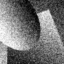
(a)	(b)	(c)	(d)

Figure 1: First-order denoising example. (a) Ground truth, (b) noisy image with additive Gaussian noise, (c) $\mathop{\rm TV}\nolimits$-regularised solution (best PSNR), (d) regularisation with smooth $\mathop{\rm TV}\nolimits$-like penalty $\varphi(x)=\sqrt{x^{2}+\varepsilon^{2}}-\varepsilon$ (best PSNR).

3.1 Symmetric tensor calculus

For smooth functions, higher-order derivatives can be represented as tensor fields, i.e., the derivative represents a tensor in each point. As the order of partial differentiation might be interchanged, these tensors turn out to be symmetric. Symmetric tensors are therefore a suitable tool for representing these objects independent from indices. There are several ways to introduce and motivate tensors and vector spaces of tensors. For our purposes, the following definition will be sufficient. Note that there and throughout this chapter, $l\geq 0$ will always be a tensor order.

Definition 3.1.

We define

$$\begin{array}[]{cc}\mathcal{T}^{l}(\mathbf{R}^{d})=\{{\xi:\underbrace{\mathbf{R}^{d}\times\cdots\times\mathbf{R}^{d}}_{l\ \mathop{\rm times}}\rightarrow\mathbf{R}}\ \bigl{|}\ {\xi\ \mbox{$l$-linear}}\},\\[6.0pt] \mathop{\rm Sym}\nolimits^{l}(\mathbf{R}^{d})=\{{\xi:\underbrace{\mathbf{R}^{d}\times\cdots\times\mathbf{R}^{d}}_{l\ \mathop{\rm times}}\rightarrow\mathbf{R}}\ \bigl{|}\ {\xi\ \mbox{$l$-linear and symmetric}}\},\end{array}$$

as the vector space of $l$-tensors and symmetric $l$-tensors, respectively.

Here, $\xi\in\mathcal{T}^{l}(\mathbf{R}^{d})$ is called symmetric, if $\xi(a_{1},\dots,a_{l})=\xi(a_{\pi(1)},\dots,a_{\pi(l)})$ for all $a_{1},\ldots a_{l}\in\mathbf{R}^{d}$ and $\pi\in S_{l}$, where $S_{l}$ denotes the permutation group of $\{{1,\ldots,l}\}$.

For $\xi\in\mathcal{T}^{k}(\mathbf{R}^{d})$, $k\geq 0$ and $\eta\in\mathcal{T}^{l}(\mathbf{R}^{d})$ the tensor product is defined as the element $\xi\otimes\eta\in\mathcal{T}^{k+l}(\mathbf{R}^{d})$ obeying

$$(\xi\otimes\eta)(a_{1},\ldots,a_{k+l})=\xi(a_{1},\ldots,a_{k})\eta(a_{k+1},\ldots,a_{k+l})$$

for all $a_{1},\ldots,a_{k+l}\in\mathbf{R}^{d}$.

Note that the space of $l$-tensors is actually the space of $(0,l)$-covariant tensors, however, we will not need to distinguish between co- and contravariant tensors. We have

$$\mathcal{T}^{0}(\mathbf{R}^{d})\equiv\mathbf{R},\quad\mathcal{T}^{1}(\mathbf{R}^{d})\equiv\mathbf{R}^{d},\quad\ldots,\quad\mathcal{T}^{l}(\mathbf{R}^{d})\equiv\mathbf{R}^{d\times\cdots\times d},$$

while for low orders, the symmetric tensor spaces coincide with well-known spaces $\mathop{\rm Sym}\nolimits^{0}(\mathbf{R}^{d})\equiv\mathbf{R}$, $\mathop{\rm Sym}\nolimits^{1}(\mathbf{R}^{d})\equiv\mathbf{R}^{d}$ and $\mathop{\rm Sym}\nolimits^{2}(\mathbf{R}^{d})\equiv S^{d\times d}$, the space of symmetric $d\times d$ matrices.

In the following, we give a brief overview of the tensor operations that are the most relevant to define regularisation functionals on higher-order derivatives.

Remark 3.2.

The space $\mathcal{T}^{l}(\mathbf{R}^{d})$ can be associated with a unit basis. Indexed by $p\in\{{1,\ldots,d}\}^{l}$, its elements are given by $e_{p}(a_{1},\ldots,a_{l})=\prod_{i=1}^{l}a_{i,p_{i}}$ while the respective coefficient for a $\xi\in\mathcal{T}^{l}(\mathbf{R}^{d})$ is given by $\xi_{p}=\xi(e_{p_{1}},\ldots,e_{p_{l}})$. Each $\xi\in\mathcal{T}^{l}(\mathbf{R}^{d})$ thus has the representation

$$\xi(a_{1},\ldots,a_{l})=\sum_{p\in\{{1,\ldots,d}\}^{l}}\xi_{p}e_{p}(a_{1},\ldots,a_{l}).$$

The identity of vector spaces $\mathcal{T}^{l}(\mathbf{R}^{d})=\mathbf{R}^{d\times\cdots\times d}$ is evident from that.

The space $\mathop{\rm Sym}\nolimits^{l}(\mathbf{R}^{d})$ is obviously a (generally proper) subspace of $\mathcal{T}^{l}(\mathbf{R}^{d})$. A (non-symmetric) tensor $\xi\in\mathcal{T}^{l}(\mathbf{R}^{d})$ can be symmetrised by averaging over all permuted arguments, i.e.,

$$(|\!|\!|\xi)(a_{1},\ldots,a_{l})=\frac{1}{l!}\sum_{\pi\in S_{l}}\xi(a_{\pi(1)},\ldots,a_{\pi(l)}).$$

The symmetrisation operator $|\!|\!|:\mathcal{T}^{l}(\mathbf{R}^{d})\to\mathop{\rm Sym}\nolimits^{l}(\mathbf{R}^{d})$ obviously defines a projection. A basis for $\mathop{\rm Sym}\nolimits^{l}(\mathbf{R}^{d})$ is given by $e^{\mathop{\rm Sym}\nolimits}_{p}=|\!|\!|e_{p}$ for $p$ ranging over all tuples in $\{{1,\ldots,d}\}^{l}$ with non-decreasing entries. The coefficients $\xi_{p}$ can still be obtained by $\xi_{p}=\xi(e_{p_{1}},\ldots,e_{p_{l}})$.

We would like to equip the spaces with a Hilbert space structure.

Definition 3.3.

For $\xi,\eta\in\mathcal{T}^{l}(\mathbf{R}^{d})$, the scalar product and Frobenius norm are defined as

$$\xi\cdot\eta=\sum_{p\in\{{1,\ldots,d}\}^{k}}\xi(e_{p_{1}},\ldots,e_{p_{l}})\eta(e_{p_{1}},\ldots,e_{p_{l}}),\qquad{|{\xi}|}=\sqrt{\xi\cdot\xi}.$$

Example 3.4.

For $\xi\in\mathop{\rm Sym}\nolimits^{l}(\mathbf{R}^{d})$, the norm corresponds to the absolute value for $l=0$, the Euclidean norm in $\mathbf{R}^{d}$ for $l=1$ and in case $l=2$, we can identify $\xi\in\mathop{\rm Sym}\nolimits^{2}(\mathbf{R}^{d})$ with

$$\xi=\left(\begin{array}[]{ccc}\xi_{11}&\cdots&\xi_{1d}\\ \vdots&\ddots&\vdots\\ \xi_{1d}&\cdots&\xi_{dd}\end{array}\right)\quad,\quad{|{\xi}|}=\Bigl{(}\sum_{i=1}^{d}\xi_{ii}^{2}+2\sum_{i<j}\xi_{ij}^{2}\Bigr{)}^{1/2}.$$

With the Frobenius norm, tensor spaces become Hilbert spaces of finite dimension and the symmetrisation becomes an orthogonal projection, see, e.g., [98].

Proposition 3.5.

1. With the above scalar-product and norm, the spaces $\mathcal{T}^{l}(\mathbf{R}^{d})$, $\mathop{\rm Sym}\nolimits^{l}(\mathbf{R}^{d})$ are finite-dimensional Hilbert spaces with $\dim\mathcal{T}^{l}(\mathbf{R}^{d})=d^{l}$ and $\dim\mathop{\rm Sym}\nolimits^{l}(\mathbf{R}^{d})={d+l-1\choose l}$.

2. The symmetrisation $|\!|\!|$ is the orthogonal projection in $\mathcal{T}^{l}(\mathbf{R}^{d})$ onto $\mathop{\rm Sym}\nolimits^{l}(\mathbf{R}^{d})$.

Tensor-valued mappings $\Omega\to\mathcal{T}^{l}(\mathbf{R}^{d})$ on the domain $\Omega\subset\mathbf{R}^{d}$ are called tensor fields. The tensor-field spaces $\mathcal{C}({\overline{\Omega},\mathcal{T}^{l}(\mathbf{R}^{d})})$, $\mathcal{C}_{\mathrm{c}}({\overline{\Omega},\mathcal{T}^{l}(\mathbf{R}^{d})})$ and $\mathcal{C}_{0}({\overline{\Omega},\mathcal{T}^{l}(\mathbf{R}^{d})})$ as well as the Lebesgue spaces $L^{p}({\Omega,\mathcal{T}^{l}(\mathbf{R}^{d})})$ are then given in the usual manner. Also, measures can be tensor-valued, giving $\mathcal{M}({\Omega,\mathcal{T}^{l}(\mathbf{R}^{d})})$, the space of $l$-tensor-valued Radon measures. Duality according to Proposition 2.4 holds, i.e., $\mathcal{M}({\Omega,\mathcal{T}^{l}(\mathbf{R}^{d})})=\mathcal{C}_{0}({\Omega,\mathcal{T}^{l}(\mathbf{R}^{d})})^{*}$. Note that for all spaces, the Frobenius norm is used as pointwise norm in the respective definitions of the tensor-field norm. Furthermore, all the above applies analogously to symmetric tensor fields, i.e., mappings between $\Omega\to\mathop{\rm Sym}\nolimits^{l}(\mathbf{R}^{d})$.

Turning to differentiation, the $k$-th Fréchet derivative of a sufficiently smooth $l$-tensor field, where from now on $k\geq 1$ will always denote an order of differentiation, is naturally a $(k+l)$-tensor field which we denote by $\nabla^{k}\otimes u:\Omega\to\mathcal{T}^{k+l}(\mathbf{R}^{d})$ according to

$$(\nabla^{k}\otimes u)(x)(a_{1},\ldots,a_{k+l})=\bigl{(}\mathrm{D}^{k}u(x)(a_{1},\ldots,a_{k})\bigr{)}(a_{k+1},\ldots,a_{k+l}).$$

The fact that gradient tensor-fields are not symmetric in general gives rise to consider the $k$-th symmetrised derivative given by $\mathcal{E}^{k}u=|\!|\!|\nabla^{k}\otimes u$. This definition is consistent as $\mathcal{E}^{k_{2}}\mathcal{E}^{k_{1}}=\mathcal{E}^{k_{1}+k_{2}}$ for $k_{1},k_{2}\geq 0$. Divergence operators are then, up to the sign, formal adjoints of these differentiation operators. They are given as follows. Introducing the trace of a tensor $\xi\in\mathcal{T}^{l+2}(\mathbf{R}^{d})$ according to

$$\tr(\xi)(a_{1},\ldots,a_{l})=\sum_{i=1}^{d}\xi(e_{i},a_{1},\ldots,a_{l},e_{i})$$

gives an $l$-tensor. It can be interpreted as the tensor contraction of the first and the last component of the tensor. As for the vector-field case, the divergence is now the trace of the derivative. For $k$-times differentiable $v:\Omega\to\mathcal{T}^{k+l}(\mathbf{R}^{d})$, the $k$-th divergence is thus given by

$$\mathop{\rm div}\nolimits^{k}v=\tr^{k}(\nabla^{k}\otimes v).$$

Again, this is consistent with repeated application, i.e., $\mathop{\rm div}\nolimits^{k_{1}+k_{2}}=\mathop{\rm div}\nolimits^{k_{2}}\mathop{\rm div}\nolimits^{k_{1}}$. Note that there might be other choices of the divergence, such as contracting the derivative with any other than the last components of the tensor. This affects, however, only non-symmetric tensor fields. For symmetric tensor fields, the result is independent from the choice of the contraction components and always a symmetric tensor field.

Example 3.6.

The symmetrised gradient of scalar functions $\Omega\to\mathop{\rm Sym}\nolimits^{0}(\mathbf{R}^{d})$ coincides with the usual gradient while the divergence for mappings $\Omega\rightarrow\mathop{\rm Sym}\nolimits^{1}(\mathbf{R}^{d})$ coincides with the usual divergence.

The cases $\mathcal{E}^{2}u^{0}$ and $\mathcal{E}u^{1}$ for $u^{0}:\Omega\to\mathop{\rm Sym}\nolimits^{0}(\mathbf{R}^{d})$ and $u^{1}:\Omega\to\mathop{\rm Sym}\nolimits^{1}(\mathbf{R}^{d})$ can be handled with the identification of $\mathop{\rm Sym}\nolimits^{2}(\mathbf{R}^{d})$ and symmetric matrices $S^{d\times d}$:

$$(\mathcal{E}^{2}u^{0})_{ij}=\frac{\partial^{2}u^{0}}{\partial x_{i}\partial x_{j}}\quad,\quad(\mathcal{E}u^{1})_{ij}=\frac{1}{2}\Bigl{(}\frac{\partial u_{i}^{1}}{\partial x_{j}}+\frac{\partial u_{j}^{1}}{\partial x_{i}}\Bigr{)}.$$

Analogously, for the divergence of a $v:\Omega\to\mathop{\rm Sym}\nolimits^{2}(\mathbf{R}^{d})$, we have that

$$(\mathop{\rm div}\nolimits v)_{i}=\sum_{j=1}^{d}\frac{\partial v_{ij}}{\partial x_{j}}\quad,\quad\mathop{\rm div}\nolimits^{2}v=\sum_{i=1}^{d}\frac{\partial^{2}v_{ii}}{\partial x_{i}^{2}}+\sum_{i<j}2\frac{\partial^{2}v_{ij}}{\partial x_{i}\partial x_{j}}.$$

In particular, for $k\geq 1$, there are the usual spaces of continuously differentiable tensor fields which are denoted by $\mathcal{C}^{k}({\overline{\Omega},\mathcal{T}^{l}(\mathbf{R}^{d})})$ and equipped with the usual norm $\|{u}\|_{k,\infty}=\max_{0\leq m\leq k}\ \|{\nabla^{m}\otimes u}\|_{\infty}$. Likewise, we consider $k$-times continuously differentiable tensor fields with compact support $\mathcal{C}_{\mathrm{c}}^{k}({\Omega,\mathcal{T}^{l}(\mathbf{R}^{d})})$ where $k=\infty$ leads to the space of test tensor fields. Also, for finite $k$, the space $\mathcal{C}_{0}^{k}({\Omega,\mathcal{T}^{l}(\mathbf{R}^{d})})$ is given as the closure of $\mathcal{C}_{\mathrm{c}}^{k}({\Omega,\mathcal{T}^{l}(\mathbf{R}^{d})})$ in $\mathcal{C}^{k}({\overline{\Omega},\mathcal{T}^{l}(\mathbf{R}^{d})})$. Of course, the analogous constructions apply to symmetric tensor fields, leading to the spaces $\mathcal{C}^{k}({\overline{\Omega},\mathop{\rm Sym}\nolimits^{l}(\mathbf{R}^{d})})$, $\mathcal{C}_{\mathrm{c}}^{k}({\Omega,\mathop{\rm Sym}\nolimits^{l}(\mathbf{R}^{d})})$ and $\mathcal{C}_{0}^{k}({\Omega,\mathop{\rm Sym}\nolimits^{l}(\mathbf{R}^{d})})$ as well as the space of test symmetric tensor fields $\mathcal{C}_{\mathrm{c}}^{\infty}({\Omega,\mathop{\rm Sym}\nolimits^{l}(\mathbf{R}^{d})})$.

As $\Omega$ is assumed to be a connected set, we are able to describe the kernels of $\nabla^{k}$ and $\mathcal{E}^{k}$ for (symmetric) tensor fields in terms of finite-dimensional spaces of polynomials.

Proposition 3.7.

Let $u\in\mathcal{C}^{k}({\overline{\Omega},\mathcal{T}^{l}(\mathbf{R}^{d})})$ such that $\nabla^{k}\otimes u=0$. Then, $u$ is a $\mathcal{T}^{l}(\mathbf{R}^{d})$-valued polynomial of maximal order $k-1$, i.e., there are $\xi^{m}\in\mathcal{T}^{l+m}(\mathbf{R}^{d})$, $m=0,\ldots,k-1$ such that

$$u(x)=\sum_{m=0}^{k-1}\tr^{m}\bigl{(}\xi^{m}\otimes(\underbrace{x\otimes\ldots\otimes x}_{m\,\mathop{times}})\bigr{)}\qquad\mbox{for each}\ x\in\Omega.$$ (8)

If $\mathcal{E}^{k}u=0$ for $u\in\mathcal{C}^{k+l}({\overline{\Omega},\mathop{\rm Sym}\nolimits^{l}(\mathbf{R}^{d})})$, then $u$ is a $\mathop{\rm Sym}\nolimits^{l}(\mathbf{R}^{d})$-valued polynomial of maximal order $k+l-1$, i.e., the above representation holds for $\xi^{m}\in\mathop{\rm Sym}\nolimits^{l+m}(\mathbf{R}^{d})$, $m=0,\ldots,k+l-1$ with the sum ranging from $0$ to $k+l-1$.

Proof.

At first we note that any $\mathcal{T}^{l}(\mathbf{R}^{d})$- and $\mathop{\rm Sym}\nolimits^{l}(\mathbf{R}^{d})$-valued polynomial of maximal order $k-1$ and $k+l-1$, respectively, admits a representation as claimed. In case $\nabla^{k}\otimes u=0$ for $u\in\mathcal{C}^{k}({\overline{\Omega},\mathcal{T}^{l}(\mathbf{R}^{d})})$ it follows directly from a basis representation of $u(x)$ that $u$ is a $\mathcal{T}^{l}(\mathbf{R}^{d})$-valued polynomial of maximal order $k-1$.

Now in case $\mathcal{E}^{k}u=0$ for $u\in\mathcal{C}^{k+l}({\overline{\Omega},\mathop{\rm Sym}\nolimits^{l}(\mathbf{R}^{d})})$, we get that $\nabla^{k+l}\otimes u=0$, see Lemma A.3. This implies that $u$ is a $\mathop{\rm Sym}\nolimits^{l}(\mathbf{R}^{d})$-valued polynomial of maximal degree $k+l-1$ as claimed. ∎

Next, we would like to introduce and discuss weak forms of differentiation for (symmetric) tensor fields. Starting point for this is a version of the well-known Gauss–Green theorem for smooth (symmetric) tensor fields [28].

Proposition 3.8.

Let $\Omega\subset\mathbf{R}^{d}$ be a bounded Lipschitz domain, $u\in\mathcal{C}({\overline{\Omega},\mathcal{T}^{l}(\mathbf{R}^{d})})$, $v\in\mathcal{C}^{1}({\overline{\Omega},\mathcal{T}^{l+1}(\mathbf{R}^{d})})$. Then, a Gauss–Green theorem holds in the following form:

$$\int_{\Omega}u\cdot\mathop{\rm div}\nolimits v\ \mathrm{d}{x}=\int_{\partial\Omega}(u\otimes\nu)\cdot v\ \mathrm{d}{\mathcal{H}^{d-1}}-\int_{\Omega}(\nabla\otimes u)\cdot v\ \mathrm{d}{x}$$

with $\nu$ being the outward unit normal on $\partial\Omega$.

If $u\in\mathcal{C}({\overline{\Omega},\mathop{\rm Sym}\nolimits^{l}(\mathbf{R}^{d})})$, $v\in\mathcal{C}^{1}({\overline{\Omega},\mathop{\rm Sym}\nolimits^{l+1}(\mathbf{R}^{d})})$, the identity reads as

$$\int_{\Omega}u\cdot\mathop{\rm div}\nolimits v\ \mathrm{d}{x}=\int_{\partial\Omega}|\!|\!|(u\otimes\nu)\cdot v\ \mathrm{d}{\mathcal{H}^{d-1}}-\int_{\Omega}\mathcal{E}u\cdot v\ \mathrm{d}{x}.$$

If one of the tensor fields $u$ or $v$ have compact support in $\Omega$ the boundary term does not appear and the identities are valid for arbitrary domains $\Omega$.

As usual, being able to express integrals of the form $\int_{\Omega}(\nabla\otimes u)\cdot v\ \mathrm{d}{x}$ and $\int_{\Omega}\mathcal{E}u\cdot v\ \mathrm{d}{x}$ for test tensor fields without the derivative of $u$ allows to introduce a weak notion of $\nabla\otimes u$ and $\mathcal{E}u$, respectively, as well as associated Sobolev spaces.

Definition 3.9.

For $u\in L^{1}_{\mathrm{loc}}({\Omega,\mathcal{T}^{l}(\mathbf{R}^{d})})$, $w\in L^{1}_{\mathrm{loc}}({\Omega,\mathcal{T}^{l+1}(\mathbf{R}^{d})})$ is the weak derivative of $u$, denoted $w=\nabla\otimes u$, if for all $\varphi\in\mathcal{C}_{\mathrm{c}}^{\infty}({\Omega,\mathcal{T}^{l+1}(\mathbf{R}^{d})})$, it holds that

$$\int_{\Omega}u\cdot\mathop{\rm div}\nolimits\varphi\ \mathrm{d}{x}=-\int_{\Omega}w\cdot\varphi\ \mathrm{d}{x}.$$

Likewise, for $u\in L^{1}_{\mathrm{loc}}({\Omega,\mathop{\rm Sym}\nolimits^{l}(\mathbf{R}^{d})})$, $w\in L^{1}({\Omega,\mathop{\rm Sym}\nolimits^{l+1}(\mathbf{R}^{d})})$ is the weak symmetrised derivative of $u$, denoted $w=\mathcal{E}u$, if the above identity holds for all $\varphi\in\mathcal{C}_{\mathrm{c}}^{\infty}({\Omega,\mathop{\rm Sym}\nolimits^{l+1}(\mathbf{R}^{d})})$.

Like the scalar versions, $\nabla$ and $\mathcal{E}$ are well-defined and constitute closed operators between the respective Lebesgue spaces with dense domain.

Definition 3.10.

The Sobolev space of tensor fields of order $l$ of differentiation order $k$ and exponent $p\in[1,\infty]$ is defined as

$$\begin{array}[]{rl}H^{k,{p}}(\Omega,\mathcal{T}^{l}(\mathbf{R}^{d}))&=\{{u\in L^{p}({\Omega,\mathcal{T}^{l}(\mathbf{R}^{d})})}\ \bigl{|}\ {\|{u}\|_{k,p}<\infty}\},\\ \|{u}\|_{k,p}&=\Bigl{(}\sum_{m=0}^{k}\|{\nabla^{m}\otimes u}\|_{p}^{p}\Bigr{)}^{1/p}\quad\mbox{if}\ p<\infty,\\ \|{u}\|_{k,\infty}&=\max_{m=0,\ldots,k}\ \|{\nabla^{m}\otimes u}\|_{\infty},\end{array}$$

while $H_{0}^{k,{p}}(\Omega,\mathcal{T}^{l}(\mathbf{R}^{d}))$ is the closure of the subspace $\mathcal{C}_{\mathrm{c}}^{\infty}({\Omega,\mathcal{T}^{l}(\mathbf{R}^{d})})$ with respect to the $\|{\,\cdot\,}\|_{k,p}$-norm.

Replacing $\mathcal{T}^{l}(\mathbf{R}^{d})$ by $\mathop{\rm Sym}\nolimits^{l}(\mathbf{R}^{d})$ and letting

$$\|{u}\|_{k,p}=\Bigl{(}\sum_{m=0}^{k}\|{\mathcal{E}^{m}u}\|_{p}^{p}\Bigr{)}^{1/p}\quad\mbox{if}\ p<\infty,\quad\|{u}\|_{\infty,k}=\max_{m=0,\ldots,k}\ \|{\mathcal{E}^{m}u}\|_{\infty},$$

defines the Sobolev space of symmetric tensor fields, denoted by $H^{k,p{}}(\Omega,\mathop{\rm Sym}\nolimits^{l}(\mathbf{R}^{d}))$. The space $H_{0}^{k,p{}}(\Omega,\mathop{\rm Sym}\nolimits^{l}(\mathbf{R}^{d}))$ is again the closure $\mathcal{C}_{\mathrm{c}}^{\infty}({\Omega,\mathop{\rm Sym}\nolimits^{l}(\mathbf{R}^{d})})$ with respect to the corresponding norm.

By closedness of the differential operators, the Sobolev spaces are Banach spaces. Also, since weak derivatives are symmetric, we have that $H^{k,p{}}(\Omega,\mathcal{T}^{0}(\mathbf{R}^{d}))=H^{k,p{}}(\Omega,\mathop{\rm Sym}\nolimits^{0}(\mathbf{R}^{d}))$ in the sense of Banach space isometry, as well as coincidence with the usual Sobolev spaces. For $l\geq 1$, the space $H^{k,p{}}(\Omega,\mathcal{T}^{l}(\mathbf{R}^{d}))$ corresponds to the space where all components of $u$ are in $H^{k,p{}}(\Omega)$. However, generally, for $l\geq 1$, the norm of $H^{k,p{}}(\Omega,\mathop{\rm Sym}\nolimits^{l}(\mathbf{R}^{d}))$ is weaker than the norm in $H^{k,p{}}(\Omega,\mathcal{T}^{l}(\mathbf{R}^{d}))$, such that only $H^{k,p{}}(\Omega,\mathcal{T}^{l}(\mathbf{R}^{d}))\hookrightarrow H^{k,p{}}(\Omega,\mathop{\rm Sym}\nolimits^{l}(\mathbf{R}^{d}))$ in the sense of continuous embedding and the latter is a strictly larger space.

Nevertheless, equality holds if some kind of Korn’s inequality can be established which is, for instance, the case for the spaces $H_{0}^{1,p{}}(\Omega,\mathop{\rm Sym}\nolimits^{1}(\mathbf{R}^{d}))$ for $1<p<\infty$ [119, Section 5.6] as well as and the spaces $H_{0}^{1,2{}}(\Omega,\mathop{\rm Sym}\nolimits^{l}(\mathbf{R}^{d}))$ for $l\geq 1$ (which follows from [28, Proposition 3.6] via smooth approximation).

Finally, let us briefly discuss (symmetric) tensor-valued distributions and the distributional forms of $\nabla^{k}$ and $\mathcal{E}^{k}$.

Definition 3.11.

A $\mathcal{T}^{l}(\mathbf{R}^{d})$-valued distribution on $\Omega$ is a linear mapping $u:\mathcal{C}_{\mathrm{c}}^{\infty}({\Omega,\mathcal{T}^{l}(\mathbf{R}^{d})})\to\mathbf{R}$ that satisfies the following continuity estimate: For each $K\subset\subset\Omega$, there is an $m\in\mathbf{N}$ and a $C>0$ such that

$${|{u(\varphi)}|}\leq C\|{\varphi}\|_{m,\infty}\qquad\mbox{for all}\ \varphi\in\mathcal{C}_{\mathrm{c}}^{\infty}({K,\mathcal{T}^{l}(\mathbf{R}^{d})}).$$

The distribution $u$ is regular if there is a $\bar{u}\in L^{1}_{\mathrm{loc}}({\Omega,\mathcal{T}^{l}(\mathbf{R}^{d})})$ such that

$$u(\varphi)=\int_{\Omega}\bar{u}\cdot\varphi\ \mathrm{d}{x}\qquad\mbox{for all}\ \varphi\in\mathcal{C}_{\mathrm{c}}^{\infty}({\Omega,\mathcal{T}^{l}(\mathbf{R}^{d})}).$$

A $\mathop{\rm Sym}\nolimits^{l}(\mathbf{R}^{d})$-valued distribution on $\Omega$ and its regularity is analogously defined by replacing $\mathcal{T}^{l}(\mathbf{R}^{d})$ by $\mathop{\rm Sym}\nolimits^{l}(\mathbf{R}^{d})$ in the above definition.

Then, the distributional (symmetrised) derivatives are given by $(\nabla^{k}\otimes u)(\varphi)=(-1)^{k}u(\mathop{\rm div}\nolimits^{k}\varphi)$, $\varphi\in\mathcal{C}_{\mathrm{c}}^{\infty}({\Omega,\mathcal{T}^{l}(\mathbf{R}^{d})})$ and $(\mathcal{E}^{k}u)(\varphi)=(-1)^{k}u(\mathop{\rm div}\nolimits^{k}\varphi)$, $\varphi\in\mathcal{C}_{\mathrm{c}}^{\infty}({\Omega,\mathop{\rm Sym}\nolimits^{l}(\mathbf{R}^{d})})$ which makes them a $\mathcal{T}^{k+l}(\mathbf{R}^{d})$- and $\mathop{\rm Sym}\nolimits^{k+l}(\mathbf{R}^{d})$-valued distribution, respectively. We then have the following generalisation of Proposition 3.7 which will be useful for analysing functionals that depend on (symmetrised) distributional derivatives.

Proposition 3.12.

If $\nabla^{k}\otimes u=0$ for a $\mathcal{T}^{l}(\mathbf{R}^{d})$-valued distribution, then $u$ is regular and a $\mathcal{T}^{l}(\mathbf{R}^{d})$-valued polynomial of maximal degree $k-1$.

If $\mathcal{E}^{k}u=0$ for a $\mathop{\rm Sym}\nolimits^{l}(\mathbf{R}^{d})$-valued distribution, then $u$ is regular and a $\mathop{\rm Sym}\nolimits^{l}(\mathbf{R}^{d})$-valued polynomial of maximal degree $k+l-1$.

Proof.

This can be deduced from Proposition 3.7 via mollification arguments similar as in [28, Proposition 3.3]. ∎

3.2 Functions of higher-order bounded variation

In the following, we discuss functions whose derivative is a Radon measure for a fixed order of differentiation. As higher-order derivatives of scalar functions are always symmetric, it suffices to consider only the symmetrised higher-order derivative $\mathcal{E}^{k}$ in this case as well as symmetric tensor fields. However, as we are also interested in intermediate differentiation orders, we moreover discuss spaces of symmetric tensors for which the symmetrised derivative of some order is a Radon measure.

In the following, recall that $k\geq 1$ denotes a differentiation order and $l\geq 0$ denotes a tensor order.

Definition 3.13.

Let $\Omega\subset\mathbf{R}^{d}$ be a domain.

1. In the case $l=0$, for $u\in L^{1}_{\mathrm{loc}}({\Omega})$, the total variation of order $k$ is defined as

   $$\mathop{\rm TV}\nolimits^{k}(u)=\sup\ \Bigl{\{}{\int_{\Omega}u\mathop{\rm div}\nolimits^{k}\varphi\ \mathrm{d}{x}}\ \Bigl{|}\ {\varphi\in\mathcal{C}_{\mathrm{c}}^{k}({\Omega,\mathop{\rm Sym}\nolimits^{k}(\mathbf{R}^{d})}),\ \|{\varphi}\|_{\infty}\leq 1}\Bigr{\}}.$$

   For general $l\geq 0$ and $u\in L^{1}_{\mathrm{loc}}({\Omega,\mathop{\rm Sym}\nolimits^{l}(\mathbf{R}^{d})})$, the total deformation of order $k$ is

   $$\mathop{\rm TD}\nolimits^{k}(u)=\sup\ \Bigl{\{}{\int_{\Omega}u\cdot\mathop{\rm div}\nolimits^{k}\varphi\ \mathrm{d}{x}}\ \Bigl{|}\ {\varphi\in\mathcal{C}_{\mathrm{c}}^{k}({\Omega,\mathop{\rm Sym}\nolimits^{k+l}(\mathbf{R}^{d})}),\ \|{\varphi}\|_{\infty}\leq 1}\Bigr{\}}.$$

2. The normed space according to

   $$\begin{array}[]{rl}\mathop{\rm BD}\nolimits^{k}(\Omega,\mathop{\rm Sym}\nolimits^{l}(\mathbf{R}^{d}))&=\{{u\in L^{1}({\Omega,\mathop{\rm Sym}\nolimits^{l}(\mathbf{R}^{d})})}\ \bigl{|}\ {\mathop{\rm TD}\nolimits^{k}(u)<\infty}\},\\ \|{u}\|_{\mathop{\rm BD}\nolimits^{k}}&=\|{u}\|_{1}+\mathop{\rm TD}\nolimits^{k}(u)\end{array}$$

   is called the space of symmetric tensor fields of bounded deformation of order $k$. The scalar case, i.e., $l=0$, is referred to as the space of functions of bounded variation of order $k$. The latter spaces are denoted by $\mathop{\rm BV}\nolimits^{k}(\Omega)$.

We note that the Hilbert-space norm on the tensor space for the definition of $\mathop{\rm TV}\nolimits^{k}$ leads to a corresponding pointwise norm on the derivatives. While this choice is rather natural, and does not require to distinguish primal and dual norms, also other choices are possible for which we refer to [127] in the second-order case.

Let us analyse some of the basic properties of these spaces.

Proposition 3.14.

Let $\Omega\subset\mathbf{R}^{d}$ be a domain, $p\in{[{1,\infty}]}$. Then:

1. $\mathop{\rm TD}\nolimits^{k}$ is proper, convex and a lower semi-continuous seminorm on $L^{p}({\Omega,\mathop{\rm Sym}\nolimits^{l}(\mathbf{R}^{d})})$.

2. $\mathop{\rm TD}\nolimits^{k}(u)=0$ if and only if $\mathcal{E}^{k}u=0$. In particular, $\mathop{\rm TD}\nolimits^{k}(u)=0$ implies that $u$ is a $\mathop{\rm Sym}\nolimits^{l}(\mathbf{R}^{d})$-valued polynomial of maximal degree $k+l-1$.

Proof.

With $p^{*}$ being the dual exponent to $p$, each test tensor field obeys $\mathop{\rm div}\nolimits^{k}\varphi\in L^{p^{*}}({\Omega,\mathop{\rm Sym}\nolimits^{l}(\mathbf{R}^{d})})$ for $\varphi\in\mathcal{C}_{\mathrm{c}}^{k}({\Omega,\mathop{\rm Sym}\nolimits^{k+l}(\mathbf{R}^{d})})$. The functional $\mathop{\rm TD}\nolimits^{k}$ is thus a pointwise supremum over a set of continuous linear functionals and, consequently, convex and lower semi-continuous. By definition, it is obviously proper and positively homogeneous since if $\mathop{\rm div}\nolimits^{k}\varphi$ is a test vector field, then also $-\mathop{\rm div}\nolimits^{k}\varphi$ is.

By definition of $\mathop{\rm TD}\nolimits^{k}$ we see that $\mathop{\rm TD}\nolimits^{k}(u)=0$ if and only if $\int_{\Omega}u\cdot\mathop{\rm div}\nolimits^{k}\varphi\ \mathrm{d}{x}=0$ for each $\varphi\in\mathcal{C}_{\mathrm{c}}^{k}({\Omega,\mathop{\rm Sym}\nolimits^{k+1}(\mathbf{R}^{d})})$. But this is equivalent to $\mathcal{E}^{k}u=0$ in the distributional sense such that in particular, the polynomial representation follows from Proposition 3.12. ∎

In order to show more properties, for instance, that $\mathop{\rm BD}\nolimits^{k}(\Omega,\mathop{\rm Sym}\nolimits^{l}(\mathbf{R}^{d}))$ is a Banach space, let us adopt a more abstract viewpoint. We say that a function ${|{\,\cdot\,}|}:X\to[0,\infty]$ for $X$ a Banach space is a lower semi-continuous seminorm on $X$ if ${|{\,\cdot\,}|}$ is positive homogeneous, satisfies the triangle inequality and is lower semi-continuous. The kernel of ${|{\,\cdot\,}|}$, denoted $\ker({{|{\,\cdot\,}|}})$, is the set $\{{x\in X}\ \bigl{|}\ {{|{x}|}=0}\}$ which is a closed linear subspace of $X$.

Lemma 3.15.

Let ${|{\,\cdot\,}|}$ be a lower semi-continuous seminorm on the Banach space $X$ with norm $\|{\,\cdot\,}\|_{X}$. Then,

$$Y=\{{x\in X}\ \bigl{|}\ {{|{x}|}<\infty}\},\qquad\|{x}\|_{Y}=\|{x}\|_{X}+{|{x}|}$$

is a Banach space. The seminorm ${|{\,\cdot\,}|}$ is continuous in $Y$.

Proof.

It is immediate that $Y$ is a normed space. Let $\{{x^{n}}\}$ be a Cauchy sequence in $Y$ which is obviously a Cauchy sequence in $X$. Hence, a limit $x\in X$ exists for which the lower semi-continuity yields ${|{x}|}\leq\liminf_{n\to\infty}{|{x^{n}}|}<\infty$, the latter since $\{{{|{x^{n}}|}}\}$ is a real Cauchy sequence. In particular, $x\in Y$.

To obtain convergence with respect to ${|{\,\cdot\,}|}$, choose, for $\varepsilon>0$, an $n$ such that for all $m\geq n$, ${|{x^{n}-x^{m}}|}\leq\varepsilon$. Letting $m\to\infty$ gives, as $x^{n}-x^{m}\to x^{n}-x$ in $X$,

$${|{x^{n}-x}|}\leq\liminf_{n\to\infty}\ {|{x^{n}-x^{m}}|}\leq\varepsilon.$$

This implies $x^{n}\to x$ in $Y$ which is what we intended to show.

Finally, the continuity of ${|{\,\cdot\,}|}$ follows from the standard estimate $\bigl{|}{{|{x^{1}}|}-{|{x^{2}}|}}\bigr{|}\leq{|{x^{1}-x^{2}}|}\leq\|{x^{1}-x^{2}}\|_{Y}$ for $x^{1},x^{2}\in Y$. ∎

It is then obvious from Proposition 3.14 and Lemma 3.15 that $\mathop{\rm BD}\nolimits^{k}(\Omega,\mathop{\rm Sym}\nolimits^{l}(\mathbf{R}^{d}))$ is a Banach space. In order to examine the structure of these spaces, it is crucial to understand the case $k=1$, i.e., $\mathop{\rm BD}\nolimits(\Omega,\mathop{\rm Sym}\nolimits^{l}(\mathbf{R}^{d}))=\mathop{\rm BD}\nolimits^{1}(\Omega,\mathop{\rm Sym}\nolimits^{l}(\mathbf{R}^{d}))$, where the symmetrised derivative is only a measure. For $l\geq 1$, these spaces are strictly greater that $\mathop{\rm BV}\nolimits(\Omega,\mathop{\rm Sym}\nolimits^{l}(\Omega))$ as a consequence of the failure of Korn’s inequality. Important properties of these spaces are summarised as follows.

Theorem 3.16 ([32, Theorem 2.6]).

If $u$ is a $\mathop{\rm Sym}\nolimits^{l}(\mathbf{R}^{d})$-valued distribution on $\Omega$ a bounded Lipschitz domain with $\mathcal{E}u\in\mathcal{M}({\Omega,\mathop{\rm Sym}\nolimits^{l+1}(\mathbf{R}^{d})})$, then $u\in\mathop{\rm BD}\nolimits(\Omega,\mathop{\rm Sym}\nolimits^{l}(\mathbf{R}^{d}))$.

Theorem 3.17 ([28, Theorems 4.16 and 4.17]).

For $\Omega$ a bounded Lipschitz domain and, $1\leq p\leq d/(d-1)$, the space $\mathop{\rm BD}\nolimits(\Omega,\mathop{\rm Sym}\nolimits^{l}(\mathbf{R}^{d}))$ is continuously embedded in $L^{p}({\Omega,\mathop{\rm Sym}\nolimits^{l}(\mathbf{R}^{d})})$. Moreover, for $p<d/(d-1)$, the embedding is compact.

Theorem 3.18 (Sobolev–Korn inequality [28, Corollary 4.20]).

For $\Omega$ a bounded Lipschitz domain and $R_{l}:L^{d/(d-1)}({\Omega,\mathop{\rm Sym}\nolimits^{l}(\mathbf{R}^{d})})\to\ker({\mathcal{E}})$ a linear and continuous projection onto the kernel of $\mathcal{E}$, there exists a constant $C>0$ such that for each $u\in\mathop{\rm BD}\nolimits(\Omega,\mathop{\rm Sym}\nolimits^{l}(\mathbf{R}^{d}))$ it follows that

$$\|{u-R_{l}u}\|_{d/(d-1)}\leq C\|{\mathcal{E}u}\|_{\mathcal{M}}.$$ (9)

Note that the projection $R_{l}$ as stated always exists as $\ker(\mathcal{E})$ is finite-dimensional (see Proposition 3.12).

Now, for general $k$ and $u\in\mathop{\rm BD}\nolimits^{k}(\Omega,\mathop{\rm Sym}\nolimits^{l}(\mathbf{R}^{d}))$ fixed, $w=\mathcal{E}^{k-1}u$ is a $\mathop{\rm Sym}\nolimits^{l+k-1}(\mathbf{R}^{d})$-valued distribution with the property

$$(\mathcal{E}w)(\varphi)=-w(\mathop{\rm div}\nolimits\varphi)=(-1)^{k}u(\mathop{\rm div}\nolimits^{k}\varphi)=(-1)^{k}\int_{\Omega}u\cdot\mathop{\rm div}\nolimits^{k}\varphi\ \mathrm{d}{x}=\int_{\Omega}\varphi\cdot\ \mathrm{d}{\mathcal{E}^{k}u}$$

for $\varphi\in\mathcal{C}_{\mathrm{c}}^{\infty}({\Omega,\mathop{\rm Sym}\nolimits^{k+l}(\mathbf{R}^{d})})$. In other words, $\mathcal{E}w=\mathcal{E}^{k}u\in\mathcal{M}({\Omega,\mathop{\rm Sym}\nolimits^{k+l}(\mathbf{R}^{d})})$, thus Theorem 3.16 implies that $\mathcal{E}^{k-1}u=w\in\mathop{\rm BD}\nolimits(\Omega,\mathop{\rm Sym}\nolimits^{k+l-1}(\mathbf{R}^{d}))$ and, in particular, we have $u\in\mathop{\rm BD}\nolimits^{k-1}(\Omega,\mathop{\rm Sym}\nolimits^{l}(\mathbf{R}^{d}))$. Hence, the spaces are nested:

$$\mathop{\rm BD}\nolimits^{k}(\Omega,\mathop{\rm Sym}\nolimits^{l}(\mathbf{R}^{d}))\subset\mathop{\rm BD}\nolimits^{k-1}(\Omega,\mathop{\rm Sym}\nolimits^{l}(\mathbf{R}^{d}))\subset\ldots\subset\mathop{\rm BD}\nolimits(\Omega,\mathop{\rm Sym}\nolimits^{l}(\mathbf{R}^{d})).$$

Let us look at the norms: By the Sobolev–Korn inequality (9), for some linear projection $R_{k+l-1}:\mathop{\rm BD}\nolimits(\Omega,\mathop{\rm Sym}\nolimits^{k+l-1}(\mathbf{R}^{d}))\to\ker({\mathcal{E}})$, we see

$$\|{\mathcal{E}^{k-1}u-R_{k+l-1}\mathcal{E}^{k-1}u}\|_{1}\leq C\|{\mathcal{E}^{k}u}\|_{\mathcal{M}}$$

which implies

$$\|{\mathcal{E}^{k-1}u}\|_{\mathcal{M}}\leq C\bigl{(}\|{\mathcal{E}^{k}u}\|_{\mathcal{M}}+\|{R_{k+l-1}\mathcal{E}^{k-1}u}\|_{1}\bigr{)}.$$

Now, $u\mapsto R_{k+l-1}\mathcal{E}^{k-1}u$ is well-defined on $\mathop{\rm BD}\nolimits^{k}(\Omega,\mathop{\rm Sym}\nolimits^{l}(\mathbf{R}^{d}))$, linear, has finite-dimensional image and is hence continuous. We may therefore estimate

$$\|{\mathcal{E}^{k-1}u}\|_{\mathcal{M}}\leq C\bigl{(}\|{u}\|_{1}+\|{\mathcal{E}^{k}u}\|_{\mathcal{M}}\bigr{)}.$$

Proceeding inductively, we arrive at the estimate

$$\sum_{m=0}^{k}\|{\mathcal{E}^{m}u}\|_{\mathcal{M}}\leq C\bigl{(}\|{u}\|_{1}+\|{\mathcal{E}^{k}u}\|_{\mathcal{M}}\bigr{)}$$ (10)

for some $C>0$ independent of $u$. Therefore, we obtain the following theorem.

Theorem 3.19.

If $\Omega\subset\mathbf{R}^{d}$ is a bounded Lipschitz domain, then the norm equivalence

$$\|{u}\|_{1}+\|{\mathcal{E}^{k}u}\|_{\mathcal{M}}\sim\sum_{m=0}^{k}\|{\mathcal{E}^{m}u}\|_{\mathcal{M}}$$ (11)

holds on $\mathop{\rm BD}\nolimits^{k}(\Omega,\mathop{\rm Sym}\nolimits^{l}(\mathbf{R}^{d}))$. The embeddings

$$\mathop{\rm BD}\nolimits^{k}(\Omega,\mathop{\rm Sym}\nolimits^{l}(\mathbf{R}^{d}))\hookrightarrow\mathop{\rm BD}\nolimits^{k-1}(\Omega,\mathop{\rm Sym}\nolimits^{l}(\mathbf{R}^{d}))\hookrightarrow\ldots\hookrightarrow\mathop{\rm BD}\nolimits(\Omega,\mathop{\rm Sym}\nolimits^{l}(\mathbf{R}^{d}))$$

are continuous.

Proof.

The nontrivial estimate to establish norm equivalence has just been shown in (10). The continuity of the embedding follows from the fact that the norm on the right-hand side in (11) is increasing with respect to $k$. ∎

In the scalar case, we can furthermore establish Sobolev embeddings.

Theorem 3.20.

Let $\Omega$ be a bounded Lipschitz domain and $0\leq m<k$.

For $k-m\leq d$:

The space $\mathop{\rm BV}\nolimits^{k}(\Omega)$ is continuously embedded in $H^{m,{p}}(\Omega)$ for $1\leq p\leq\frac{d}{d-(k-m)}$, where we set $\frac{d}{d-(k-m)}=\infty$ for $k-m=d$.

If $p<\frac{d}{d-(k-m)}$, then the embedding is compact.

For $k-m>d$:

The space $\mathop{\rm BV}\nolimits^{k}(\Omega)$ is compactly embedded in $\mathcal{C}^{m,\alpha}({\overline{\Omega}})$ for each $\alpha\in{]{0,1}[}$.

Proof.

In the scalar case, $\|{u}\|_{1}+\sum_{{|{\beta}|}\leq k-1}\|{\nabla\partial^{\beta}u}\|_{\mathcal{M}}$ for $\beta\in\mathbf{N}^{d}$ a multiindex and $u\in\mathop{\rm BV}\nolimits^{k}(\Omega)$ constitutes an equivalent norm on $\mathop{\rm BV}\nolimits^{k}(\Omega)$, as a consequence of Theorem 3.19. By the Poincaré inequality in $\mathop{\rm BV}\nolimits(\Omega)$,

$$\|{\partial^{\beta}u}\|_{d/(d-1)}\leq C\bigl{(}\|{\nabla\partial^{\beta}u}\|_{\mathcal{M}}+\|{u}\|_{1}\bigr{)}$$

for each ${|{\beta}|}\leq k-1$. This establishes the continuous embedding $\mathop{\rm BV}\nolimits^{k}(\Omega)\to W^{k-1,d/(d-1)}(\Omega)$. Application of the well-known embedding theorems for Sobolev spaces (see [1, Theorems 5.4 and 6.2]) then give the results for the cases $k-m<d$ and $k-m>d$ as well as for the case $k-m=d$ and $p<\infty$.

For the case $k-m=d$ and $p=\infty$ we note that again by Sobolev embeddings [1, Theorem 5.4] we get for a constant $C>0$ and all $u\in H^{k,{1}}(\Omega)$ that

$$\sum_{i=0}^{m}\|{\nabla^{i}u}\|_{\infty}\leq C\sum_{i=0}^{k}\|{\nabla^{i}u}\|_{1}.$$

Approximating $u\in\mathop{\rm BV}\nolimits^{k}(\Omega)$ with a sequence $\{{u^{n}}\}$ in $C^{\infty}(\Omega)\cap\mathop{\rm BV}\nolimits^{k}(\Omega)$ strictly converging to $u$ in $\mathop{\rm BV}\nolimits^{k}(\Omega)$ as in Lemma A.4, the result follows from applying this estimate to each $u^{n}$ and using lower semi-continuity of the $L^{\infty}$-norm with respect to convergence in $L^{1}$. ∎

We would like to employ $\mathop{\rm TD}\nolimits^{k}$ as a regulariser and first characterise its kernel. For that purpose, we note that $\mathop{\rm TD}\nolimits^{k}(u)=0$ for some $u\in\mathop{\rm BD}\nolimits^{k}(\Omega,\mathop{\rm Sym}\nolimits^{l}(\mathbf{R}^{d}))$ implies that $\mathcal{E}u=0$ in the distributional sense, hence Proposition 3.12 implies that $u$ is a $\mathop{\rm Sym}\nolimits^{l}(\mathbf{R}^{d})$-valued polynomial of maximal degree $k+l-1$. This yields the following result.

Proposition 3.21.

The space $\ker({\mathop{\rm TD}\nolimits^{k}})$ is a subspace of polynomials of degree less than $k+l$. If $l=0$, then $\ker({\mathop{\rm TV}\nolimits^{k}})=\mathbf{P}^{k-1}=\{{u:\Omega\to\mathbf{R}}\ \bigl{|}\ {u\ \mbox{polynomial of degree}\leq k-1}\}$.

Next, we like to discuss coercivity of the higher-order total variation functionals.

Proposition 3.22.

Let $k\geq 1$, $l\geq 0$ and $\Omega$ be a bounded Lipschitz domain. Then, $\mathop{\rm TD}\nolimits^{k}$ is coercive in the following sense: For each linear and continuous projection $R:L^{d/(d-1)}({\Omega,\mathop{\rm Sym}\nolimits^{l}(\mathbf{R}^{d})})\to\ker({\mathop{\rm TD}\nolimits^{k}})$, there is a $C>0$ such that

$$\|{u-Ru}\|_{d/(d-1)}\leq C\mathop{\rm TD}\nolimits^{k}(u)\qquad\mbox{for all}\quad u\in\mathop{\rm BD}\nolimits^{k}(\Omega,\mathop{\rm Sym}\nolimits^{l}(\mathbf{R}^{d})).$$

Proof.

At first note that by the embeddings $\mathop{\rm BD}\nolimits^{k}(\Omega,\mathop{\rm Sym}\nolimits^{l}(\mathbf{R}^{d}))\hookrightarrow\mathop{\rm BD}\nolimits(\Omega,\mathop{\rm Sym}\nolimits^{l}(\mathbf{R}^{d}))\hookrightarrow L^{d/(d-1)}({\Omega,\mathop{\rm Sym}\nolimits^{l}(\mathbf{R}^{d})})$ the left hand side of the claimed inequality is well defined and finite.

We use a contradiction argument in conjunction with compactness. Suppose for $R$ as stated above there is a sequence $\{{u^{n}}\}$ such that $\|{u^{n}-Ru^{n}}\|_{d/(d-1)}=1$ and $\mathop{\rm TD}\nolimits^{k}(u^{n})\to 0$ as $n\to\infty$. This implies $\{{\|{u^{n}-Ru^{n}}\|_{1}}\}$ being bounded, $\mathop{\rm TD}\nolimits^{k}(u^{n}-Ru^{n})\to 0$ and by Theorems 3.19 and 3.17 $\{{u^{n}-Ru^{n}}\}$ has to be precompact in $L^{1}({\Omega,\mathop{\rm Sym}\nolimits^{l}(\mathbf{R}^{d})})$, i.e., without loss of generality, we may assume that $u^{n}-Ru^{n}\to u$ in $L^{1}({\Omega,\mathop{\rm Sym}\nolimits^{l}(\mathbf{R}^{d})})$. By lower semi-continuity,

$$\mathop{\rm TD}\nolimits^{k}(u)\leq\liminf_{n\to\infty}\ \mathop{\rm TD}\nolimits^{k}(u^{n})=0,$$

hence $u\in\ker({\mathop{\rm TD}\nolimits^{k}})=\mathop{\rm rg}\nolimits({R})$. On the other hand, $R(u^{n}-Ru^{n})=0$ for each $n$ as $R$ is a projection, thus, $Ru=0$ and, consequently, $u=0$. In total, we have $\lim_{n\to\infty}(u^{n}-Ru^{n})=0$ in $\mathop{\rm BD}\nolimits^{k}(\Omega)$, and again by continuous embedding, also in $L^{d/(d-1)}({\Omega})$ which is a contradiction to $\|{u^{n}-Ru^{n}}\|_{d/(d-1)}=1$ for all $n$. Consequently, coercivity has to hold. ∎

Corollary 3.23.

In the scalar case, for $p\in[1,\infty]$ with $p\leq\frac{d}{d-k}$ if $k<d$, we also have

$$\|{u-Ru}\|_{p}\leq C\mathop{\rm TV}\nolimits^{k}(u).$$

Proof.

This follows with the embedding Theorem 3.20:

$$\|{u-Ru}\|_{p}\leq C\bigl{(}\|{u-Ru}\|_{1}+\mathop{\rm TV}\nolimits^{k}(u)\bigr{)}\leq C\mathop{\rm TV}\nolimits^{k}(u).\qed$$

Remark 3.24.

The above coercivity estimate also implies that the Fenchel conjugate of $\mathop{\rm TV}\nolimits^{k}$ is the indicator functional of closed convex set in $L^{p^{*}}({\Omega})\cap\ker({\mathop{\rm TV}\nolimits^{k}})^{\perp}$ with non-empty interior. Indeed, for $\xi\in L^{p^{*}}({\Omega})\cap\ker({\mathop{\rm TV}\nolimits^{k}})^{\perp}$ such that $\|{\xi}\|_{p^{*}}\leq C^{-1}$ it follows for any $u\in L^{p}({\Omega})$ that

$$\langle{\xi},\,{u}\rangle=\langle{\xi},\,{u-Ru}\rangle\leq\|{\xi}\|_{p^{*}}\|{u-Ru}\|_{p}\leq\mathop{\rm TV}\nolimits^{k}(u)$$

which means that $(\mathop{\rm TV}\nolimits^{k})^{*}(\xi)=0$. On the other hand, if $\xi\in L^{p^{*}}({\Omega})\setminus\ker({\mathop{\rm TV}\nolimits^{k}})^{\perp}$, then $\langle{\xi},\,{u}\rangle>0$ for some $u\in\ker({\mathop{\rm TV}\nolimits^{k}})$. Thus, $\langle{\xi},\,{u}\rangle>\mathop{\rm TV}\nolimits^{k}(u)$ so $(\mathop{\rm TV}\nolimits^{k})^{*}(\xi)=\infty$.

It is interesting to note that a coercivity estimate similar to the one of Corollary 3.23 also holds between two higher-order TV functionals of different order.

Lemma 3.25.

Let $\Omega$ be a bounded Lipschitz domain, $1\leq k_{1}<k_{2}$ be two orders of differentiation, $p\in[1,\infty[$ with $p\leq d/(d-k_{2})$ if $k_{2}<d$ and $R:L^{p}(\Omega)\rightarrow\ker(\mathop{\rm TV}\nolimits^{k_{2}})$ be a continuous, linear projection. Then there exists a constant $C>0$ such that

$$\mathop{\rm TV}\nolimits^{k_{1}}(u-Ru)\leq C\mathop{\rm TV}\nolimits^{k_{2}}(u)$$ (12)

holds for each $u\in\mathop{\rm BV}\nolimits^{k_{2}}(\Omega)$.

Proof.

Assume the opposite, i.e., the existence of $\{{u^{n}}\}$ such that $\mathop{\rm TV}\nolimits^{k_{1}}(u^{n}-Ru^{n})=1$ and $\mathop{\rm TV}\nolimits^{k_{2}}(u^{n})\to 0$ as $n\to\infty$. Then, by compact embedding $\mathop{\rm BD}\nolimits^{k_{2}-k_{1}}(\Omega,\mathop{\rm Sym}\nolimits^{k_{1}}(\mathbf{R}^{d}))\to L^{1}({\Omega,\mathop{\rm Sym}\nolimits^{k_{1}}(\mathbf{R}^{d})})$, we have $\nabla^{k_{1}}(u^{n}-Ru^{n})\to v$ as $n\to\infty$ for some $v\in L^{1}({\Omega,\mathop{\rm Sym}\nolimits^{k_{1}}(\mathbf{R}^{d})})$ for a subsequence (not relabelled). On the other hand, the Poincaré estimate gives $\|{u^{n}-Ru^{n}}\|_{p}\leq C\mathop{\rm TV}\nolimits^{k_{2}}(u^{n})$, so $u^{n}-Ru^{n}\to 0$ as $n\to\infty$ in $L^{1}({\Omega})$. By closedness of $\nabla^{k_{1}}$ this yields $v=0$. By convergence in $L^{1}({\Omega,\mathop{\rm Sym}\nolimits^{k_{1}}(\mathbf{R}^{d})})$, this gives the contradiction $\mathop{\rm TV}\nolimits^{k_{1}}(u^{n}-Ru^{n})\to 0$ as $n\to\infty$. ∎

3.3 Tikhonov regularisation

The coercivity which has just been established can be regarded as the most important step towards existence for variational problems with $\mathop{\rm TV}\nolimits^{k}$-regularisation. Here, we first prove an existence result for linear inverse problems in a general abstract version.

Theorem 3.26.

Let $X$ be a reflexive Banach space, $Y$ be a Banach space, $K:X\to Y$ be linear and continuous, $S_{f}:Y\to{[{0,\infty}]}$ a proper, convex, lower semi-continuous and coercive discrepancy functional associated with some data $f$, ${|{\,\cdot\,}|}:X\rightarrow[0,\infty]$ a lower semi-continuous seminorm and $\alpha>0$. Assume that there exists a linear and continuous projection $R:X\rightarrow\ker({|{\,\cdot\,}|})$ and a $C>0$ such that

$$\|{u-Ru}\|_{X}\leq C{|{u}|}\qquad\mbox{for all}\quad u\in X,$$

and either

1. $\ker({|{\,\cdot\,}|})$ is finite-dimensional or, more generally,

2. $\ker(K)\cap\ker({|{\,\cdot\,}|})$ admits a complement $Z$ in $\ker({|{\,\cdot\,}|})$ and $\|{u}\|_{X}\leq C\|{Ku}\|_{Y}$ for some $C>0$ and all $u\in Z$.

Then, the Tikhonov minimisation problem

$$\min_{u\in X}\ S_{f}(Ku)+\alpha{|{u}|}.$$ (13)

is well-posed, i.e., there exists a solution and the solution mapping is stable in sense that, if $S_{f^{n}}$ converges to $S_{f}$ as in (4) and $\{{S_{f^{n}}}\}$ is equi-coercive, then for each sequence of minimizers $\{{u^{n}}\}$ of (13) with discrepancy $S_{f^{n}}$,

• either $S_{f^{n}}(Ku^{n})+\alpha{|{u^{n}}|}\to\infty$ as $n\to\infty$ and (13) with discrepancy $S_{f}$ does not admit a finite solution,

• or $S_{f^{n}}(Ku^{n})+\alpha{|{u^{n}}|}\to\min_{u\in X}S_{f}(u)+\alpha{|{u}|}$ as $n\to\infty$ and there is, possibly up to shifts by functions in $\ker(K)\cap\ker({|{\,\cdot\,}|})$, a weak accumulation point $u\in X$ that minimises (13) with discrepancy $S_{f}$.

Further, in case (13) with discrepancy $S_{f}$ admits a finite solution, for each subsequence $\{{u^{n_{k}}}\}$ weakly converging to some $u\in X$, it holds that ${|{u^{n_{k}}}|}\to{|{u}|}$ as $k\to\infty$. Also, if $S_{f}$ is strictly convex and $K$ is injective, finite solutions $u$ of (13) are unique and $u^{n}\rightharpoonup u$ in $X$.

The same result is true if, for instance, instead of being reflexive, $X$ is the dual of a separable space, and we replace weak convergence by weak* convergence in the (lower semi-) continuity assumptions on $K$, ${|{\,\cdot\,}|}$, $S_{f}$ and in (4).

Proof.

At first note that $\ker({|{\,\cdot\,}|})$ being finite-dimensional implies condition (ii) above, hence we can assume that (ii) holds. We start with existence. Assume that the objective functional in (13) is proper as otherwise, there is nothing to show. For a minimising sequence $\{{u^{n}}\}$, by the coercivity assumption, $\{{u^{n}-Ru^{n}}\}$ is bounded in $X$. Now, (ii) implies the existence of a linear and continuous projection $P_{Z}:\ker({|{\,\cdot\,}|})\to Z$ such that $\mathop{\rm id}\nolimits-P_{Z}$ projects $\ker({|{\,\cdot\,}|})$ onto $\ker(K)\cap\ker({|{\,\cdot\,}|})$. With $v^{n}=P_{Z}Ru^{n}$, we see that also $\{{u^{n}-Ru^{n}+v^{n}}\}$ is a minimising sequence and it suffices to show boundedness of $\{{v^{n}}\}$ to obtain a convergent subsequence. But the latter holds true since by assumption $\|{v^{n}}\|_{p}\leq C\|{Kv^{n}}\|_{Y}$, such that $\|{Kv^{n}}\|_{Y}\leq\|{K(u^{n}-Ru^{n}+v^{n})}\|_{Y}+\|{K}\|\|{u^{n}-Ru^{n}}\|_{X}$, with the right-hand side being bounded as a consequence of the coercivity of $S_{f}$ and the boundedness of $\{{u^{n}-Ru^{n}}\}$. Hence, as $X$ is reflexive, a subsequence of $\{{u^{n}-Ru^{n}+v^{n}}\}$ converges weakly to a limit $u\in X$. By continuity of $K$ and lower semi-continuity of both $S_{f}$ and ${|{\,\cdot\,}|}$ it follows that $u$ is a solution to (13). In case $S_{f}$ is strictly convex and $K$ is injective, $S_{f}\circ K$ is already strictly convex, so finite minimizers of (13) have to be unique.

Now let $\{{u^{n}}\}$ be a sequence of minimizers of (13) with discrepancy $S_{f^{n}}$. We denote by $F=S_{f}\circ K+\alpha{|{\,\cdot\,}|}$ as well as $F_{n}=S_{f^{n}}\circ K+\alpha{|{\,\cdot\,}|}$ and first suppose that $\{{F_{n}(u^{n})}\}$ is bounded. We can then add $v^{n}-Ru^{n}\in\ker(K)\cap\ker({|{\,\cdot\,}|})$ to $u^{n}$, with $v^{n}=P_{Z}Ru^{n}$, and from equi-coercivity of $\{{S_{f^{n}}}\}$ obtain boundedness of $\{{u^{n}-Ru^{n}+v^{n}}\}$ as before. This shows that by shifting the minimizers within $\ker(K)\cap\ker({|{\,\cdot\,}|})$ always leads to a bounded sequence, i.e., we may assume without loss of generality that $\{{u^{n}}\}$ is bounded such that a weak accumulation point exists. Suppose that $u^{n_{k}}\rightharpoonup u$ as $k\to\infty$. Then, estimating as in the proof of Theorem 2.14, we can obtain that $u$ is a minimizer for $F$ and that $\lim_{k\to\infty}F_{n_{k}}(u^{n_{k}})=F(u)$ as well as $\lim_{k\to\infty}{|{u^{n_{k}}}|}={|{u}|}$. Also, if $u$ is the unique minimizer for (13) with discrepancy $S_{f}$, $u^{n}\rightharpoonup u$ as $n\to\infty$ follows since any subsequence has to contain another subsequence that converges weakly to $u$.

The result for the two remaining cases $\liminf_{n\to\infty}F_{n}(u^{n})<\infty$ and $F_{n}(u^{n})\to\infty$, respectively, finally follows analogously to Theorem 2.14. ∎

Given that $\ker(\mathop{\rm TV}\nolimits^{k})$ is finite dimensional, the above result immediately implies well-posedness for ${|{\,\cdot\,}|}=\mathop{\rm TV}\nolimits^{k}$ with $X=L^{p}({\Omega})$, as stated in the following corollary. The crucial ingredient here is the estimate $\|{u-Ru}\|_{p}\leq C\mathop{\rm TV}\nolimits^{k}(u)$, which restricts the exponent of the underlying $L^{p}$-space to $p\leq d/(d-k)$ if $k<d$. This shows that, the higher the order of differentiation used in the regularisation, the weaker are the requirements on the underlying spaces and, consequently, on the continuity of the operator $K$.

Corollary 3.27.

With $X=L^{p}(\Omega)$, $\Omega$ being a bounded Lipschitz domain, and $S_{f}$ and $K$ as in Theorem 3.26,

$$\min_{u\in L^{p}({\Omega})}\ S_{f}(Ku)+\alpha\mathop{\rm TV}\nolimits^{k}(u).$$ (14)

is well-posed in the sense of Theorem 3.26 whenever $p\in{]{1,\infty}[}$ with $p\leq d/(d-k)$ if $k<d$.

As can be easily seen from the respective proofs, also the convergence result of Theorem 2.17 and the result on convergence rates as in Proposition 2.18 transfer to $\mathop{\rm TV}\nolimits^{k}$ regularisation.

Theorem 3.28.

With the assumptions of Corollary 3.27, let $u^{\dagger}\in\mathop{\rm BV}\nolimits(\Omega)$ be a minimum-$\mathop{\rm TV}\nolimits^{k}$-solution of $Ku^{\dagger}=f^{\dagger}$ for some data $f^{\dagger}$ in $Y$ and for each $\delta>0$ let $f^{\delta}$ be such that $S_{f^{\delta}}(f^{\dagger})\leq\delta$ and denote by $u^{\alpha,\delta}$ a finite solution of (14) for parameter $\alpha>0$ and data $f^{\delta}$. Let the discrepancy functionals $\{{S_{f^{\delta}}}\}$ be equi-coercive and converge to $S_{f^{\dagger}}$ in the sense of (4) and $S_{f^{\dagger}}(v)=0$ if and only if $v=f^{\dagger}$. Choose for each $\delta>0$ the parameter $\alpha>0$ such that

$$\alpha\to 0,\quad\frac{\delta}{\alpha}\to 0\qquad\mbox{as}\qquad\delta\to 0.$$

Then, up to shifts by functions in $\ker(K)\cap\mathbf{P}^{k-1}$, $\{{u^{\alpha,\delta}}\}$ has at least one $L^{p}$-weak accumulation point. Each $L^{p}$-weak accumulation point is a minimum-$\mathop{\rm TV}\nolimits^{k}$-solution of $Ku=f^{\dagger}$ and $\lim_{\delta\to 0}\mathop{\rm TV}\nolimits^{k}(u^{\alpha,\delta})=\mathop{\rm TV}\nolimits^{k}(u^{\dagger})$.

Proposition 3.29.

In the situation of Theorem 3.28, let $K^{*}w^{\dagger}\in\partial\mathop{\rm TV}\nolimits^{k}(u^{\dagger})$ for some $w^{\dagger}\in Y^{*}$. Then,

$$D^{\mathop{\rm TV}\nolimits^{k}}_{K^{*}w^{\dagger}}(u^{\alpha,\delta},u^{\dagger})\leq\frac{1}{\alpha}\bigl{(}S_{f^{\delta}}^{*}(\alpha w^{\dagger})+S_{f^{\delta}}^{*}(-\alpha w^{\dagger})+2\delta\bigr{)}.$$ (15)

The last result in particular guarantees convergence rates for the settings of Example 2.19. Note also that the above results remain true in case $p=1$ or in case $p=d/(d-k)=\infty$ and $K$ is weak*-to-weak continuous.

Let us finally note some first-order optimality conditions. For this purpose, recall that for $X$ a Banach space, the normal cone $\mathcal{N}_{K}(u)$ of a set $K\subset X$ at $u\in K$ is given by the collection of all $w\in X^{*}$ for which $\langle{w},\,{v-u}\rangle_{X^{*}\times X}\leq 0$ for all $v\in K$. If we set $\mathcal{N}_{K}(u)=\emptyset$ for $u\notin K$, we have that $\mathcal{N}_{K}=\partial\mathcal{I}_{K}$ where $\mathcal{I}_{K}$ is the indicator function of $K$, i.e., $\mathcal{I}_{K}(u)=0$ if $u\in K$ and $\infty$ otherwise.

Proposition 3.30.

In the situation of Corollary 3.27, if $S_{f}(v)=\frac{1}{2}\|v-f\|_{Y}^{2}$ and $Y$ is a Hilbert space, $u^{*}\in L^{p}({\Omega})$ is a solution of

$$\min_{u\in L^{p}({\Omega})}\ \frac{1}{2}\|{Ku-f}\|_{Y}^{2}+\alpha\mathop{\rm TV}\nolimits^{k}(u)$$ (16)

if and only if

$$u^{*}\in\mathcal{N}_{\mathop{\rm TV}\nolimits^{k}}\Bigl{(}\frac{K^{*}(f-Ku^{*})}{\alpha}\Bigr{)}$$

where $\mathcal{N}_{\mathop{\rm TV}\nolimits^{k}}$ is the normal cone associated with the set $\overline{\mathcal{B}_{\mathop{\rm TV}\nolimits^{k}}}$ where

$$\mathcal{B}_{\mathop{\rm TV}\nolimits^{k}}=\{{w\in L^{p^{*}}({\Omega})}\ \bigl{|}\ {w=\mathop{\rm div}\nolimits^{k}\varphi,\ \varphi\in\mathcal{C}_{\mathrm{c}}^{k}({\Omega,\mathop{\rm Sym}\nolimits^{k}(\mathbf{R}^{d})}),\ \|{\varphi}\|_{\infty}\leq 1}\}.$$

Proof.

As $u\mapsto\frac{1}{2}\|{Ku-f}\|_{Y}^{2}$ is Gâteaux differentiable, it is continuous with unique subgradient, so, by subdifferential calculus, optimality of $u^{*}$ is equivalent to $K^{*}(f-Ku^{*})\in\alpha\partial\mathop{\rm TV}\nolimits^{k}(u^{*})$ which can also be expressed as

$$u^{*}\in\partial(\mathop{\rm TV}\nolimits^{k})^{*}\Bigl{(}\frac{K^{*}(f-Ku^{*})}{\alpha}\Bigr{)}.$$

Now since $\mathop{\rm TV}\nolimits^{k}=\mathcal{I}_{\mathcal{B}_{\mathop{\rm TV}\nolimits^{k}}}^{*}$, it follows that $(\mathop{\rm TV}\nolimits^{k})^{*}=\mathcal{I}_{\mathcal{B}_{\mathop{\rm TV}\nolimits^{k}}}^{**}=\mathcal{I}_{\overline{\mathcal{B}_{\mathop{\rm TV}\nolimits^{k}}}}$ , so $\partial(\mathop{\rm TV}\nolimits^{k})^{*}=\mathcal{N}_{\mathop{\rm TV}\nolimits^{k}}$. ∎

Remark 3.31.

In the situation of Proposition 3.30, it is also possible to give an a-priori estimate for the solutions of (16) in case $K$ is injective on $\mathbf{P}^{k-1}$. Indeed, with $R:L^{p}({\Omega})\to\mathbf{P}^{k-1}$ the continuous projection operator on the kernel of $\mathop{\rm TV}\nolimits^{k}$ and $C>0$ the coercivity constant, i.e., $\|{u-Ru}\|_{p}\leq C\mathop{\rm TV}\nolimits^{k}(u)$ for all $u\in L^{p}({\Omega})$, by optimality, a solution $u^{*}$ satisfies $\alpha\mathop{\rm TV}\nolimits^{k}(u^{*})\leq\frac{1}{2}\|{f}\|_{Y}^{2}$ and consequently, $\|{u-Ru}\|_{p}\leq\frac{1}{2\alpha}C\|{f}\|_{Y}^{2}$. Likewise, comparing with $u^{*}-Ru^{*}$, optimality also gives $\|{Ku^{*}-f}\|_{Y}^{2}\leq\|{K(u^{*}-Ru^{*})-f}\|_{Y}^{2}$, which is equivalent to $\|{KRu^{*}}\|_{Y}^{2}\leq 2\langle{KRu^{*}},\,{f-K(u^{*}-Ru^{*})}\rangle$. Using $ab\leq\frac{1}{4}a^{2}+b^{2}$, the latter leads to $\|{KRu^{*}}\|_{Y}^{2}\leq 4\|{f-K(u^{*}-Ru^{*})}\|_{Y}^{2}$, where the right-hand side can further be estimated, using $(a+b)^{2}\leq(1+\varepsilon)(a^{2}+\frac{1}{\varepsilon}b^{2})$ with $\varepsilon=\frac{1}{4\alpha^{2}}C^{2}\|{K}\|^{2}$ to give

$$\|{KRu^{*}}\|_{Y}^{2}\leq 4\Bigl{(}1+\frac{C^{2}\|{K}\|^{2}}{4\alpha^{2}}\Bigr{)}(1+\|{f}\|_{Y}^{2})\|{f}\|_{Y}^{2}.$$

Now, as $K$ is injective on $\mathbf{P}^{k-1}=\mathop{\rm rg}\nolimits({R})$, there is a $c>0$ such that $c\|{Ru}\|_{p}\leq\|{KRu}\|_{Y}$ for all $u\in L^{p}({\Omega})$. Consequently, employing the triangle inequality and estimating yields

$$\|{u^{*}}\|_{p}\leq\frac{1}{2\alpha}\Bigl{(}\frac{2}{c}\sqrt{4\alpha^{2}+C^{2}\|{K}\|^{2}}+C\Bigr{)}\sqrt{1+\|{f}\|_{Y}^{2}}\|{f}\|_{Y},$$ (17)

which is an a-priori bound that only requires the knowledge of the Poincaré–Wirtinger-type constant $C$, the constant $c$ in the inverse estimate for $K$ on $\mathbf{P}^{k+1}$, as well as an estimate on $\|{K}\|$. Beyond being of theoretical interest, such a bound can for instance be used in numerical algorithms, see Section 6, Example 6.23.

If the Kullback–Leibler divergence is used instead of the quadratic Hilbert space discrepancy, i.e., $S_{f}(v)=\mathop{\rm KL}\nolimits(v,f)$, $Y=L^{1}({\Omega^{\prime}})$, and data $f\geq 0$ a.e., then one has to choose a $u^{0}\in\mathop{\rm BV}\nolimits^{k}(\Omega)$ such that $\mathop{\rm KL}\nolimits(Ku^{0},f)<\infty$. Set $C_{f}=\mathop{\rm KL}\nolimits(Ku^{0},f)+\alpha\mathop{\rm TV}\nolimits^{k}(u^{0})$. Then, an optimal solution $u^{*}$ will satisfy $\mathop{\rm TV}\nolimits^{k}(u^{*})\leq\frac{C_{f}}{\alpha}$. Further, we have $\|{v}\|_{1}\leq 2\mathop{\rm KL}\nolimits(v,f)+2\|{f}\|_{1}$ for $v\in L^{1}({\Omega^{\prime}})$ with $v\geq 0$ a.e., see Lemma A.1, such that, if $c>0$ is a constant with $c\|{Ru}\|_{p}\leq\|{KRu}\|_{1}$ for all $u\in L^{p}({\Omega})$, we get

$$\|{Ru^{*}}\|_{p}\leq\frac{1}{c}\bigl{(}\|{Ku^{*}}\|_{1}+\|{K}\|\|{u^{*}-Ru^{*}}\|_{p}\bigr{)}\leq\frac{1}{c}\Bigl{(}\frac{2\alpha+C\|{K}\|}{\alpha}C_{f}+2\|{f}\|_{1}\Bigr{)},$$

and finally arrive at

$$\|{u^{*}}\|_{p}\leq\frac{1}{c}\Bigl{(}\frac{2\alpha+C\|{K}\|+cC}{\alpha}C_{f}+2\|{f}\|_{1}\Bigr{)}.$$ (18)

This constitutes an a-priori estimate similar to (17) for the Kullback–Leibler discrepancy, however, with the difference that also a suitable constant $C_{f}$ has to determined.

(a)	(b)	(c)	(d)

Figure 2: Second-order total-variation denoising example. (a) Noisy image, (b) regularisation with $\mathop{\rm TV}\nolimits$, (c) regularisation with $\mathop{\rm TV}\nolimits^{2}$, (d) regularisation with $\|{\Delta\,\cdot\,}\|_{\mathcal{M}}$. All parameters are tuned to give highest PSNR with respect to the ground truth (Figure 1 (a)).

Remark 3.32.

In order to show the effect of $\mathop{\rm TV}\nolimits^{2}$ regularisation in contrast to $\mathop{\rm TV}\nolimits$ regularisation, we performed a numerical denoising experiment for $f$ shown in Figure 2 (a), i.e., solved $\min_{u\in L^{2}({\Omega})}\frac{1}{2}\|{u-f}\|_{2}^{2}+\mathcal{R}_{\alpha}(u)$ where $\mathcal{R}_{\alpha}=\alpha\mathop{\rm TV}\nolimits$ or $\mathcal{R}_{\alpha}=\alpha\mathop{\rm TV}\nolimits^{2}$. One clearly sees that $\mathop{\rm TV}\nolimits^{2}$ regularisation (Figure 2 (c)) reduces the staircasing effect of $\mathop{\rm TV}\nolimits$ regularisation (Figure 2 (b)) and piecewise linear structures are well recovered. However, $\mathop{\rm TV}\nolimits^{2}$ regularisation also blurs the object boundaries which appear less sharp in contrast to $\mathop{\rm TV}\nolimits$ regularisation.

This is due to the fact that $\mathop{\rm TV}\nolimits^{k}$ regularisation for $k\geq 2$ is not able to produce solutions with jump discontinuities. Indeed, $\mathop{\rm TV}\nolimits^{k}$ regularisation implies that a solution $u$ has be to contained in $\mathop{\rm BV}\nolimits^{k}(\Omega)$ which embeds into the Sobolev space $H^{k-1,{1}}(\Omega)\hookrightarrow H^{1,{1}}(\Omega)$. As we have seen, for instance, in Example 2.1, this means that characteristic functions cannot be solutions. More generally, for $u\in H^{1,{1}}(\Omega)\subset\mathop{\rm BV}\nolimits(\Omega)$, the derivative $\nabla u$ interpreted as a measure is absolutely continuous with respect to the Lebesgue measure such that the singular part satisfies $\nabla^{s}u=0$. Theorem 2.21 then implies that the jump set $J_{u}$ is a $\mathcal{H}^{d-1}$-negligible set, i.e., $u$ cannot jump on $(d-1)$-dimensional hypersurfaces.

Remark 3.33.

Instead of taking higher-order TV which bases on the full gradient, one could also try to regularise with other differential operators, for instance with the (weak) Laplacian:

$$\mathcal{R}_{\alpha}(u)=\alpha\|{\Delta u}\|_{\mathcal{M}}.$$

However, the kernel of this seminorm is the space of $p$-integrable harmonic functions on $\Omega$, the Bergman spaces, which are infinite-dimensional. Therefore, in view of Theorem 3.26, to use $\mathcal{R}_{\alpha}$ for the regularisation of ill-posed linear inverse problems, the forward operator $K$ must be continuously invertible on a complement of $\ker({\mathcal{R}_{\alpha}})\cap\ker(K)$, i.e., well-posed. This limits the applicability of this regulariser. Nevertheless, denoising problems can, for instance, still be solved, see Figure 2 (d), leading to “speckle” artefacts in the solutions. Another possibility would be to add more regularising functionals, which is discussed in the next section.

Higher order TV for multichannel images.

In analogy to TV, also higher order TV can be extended to colour and multichannel images represented by functions mapping into a vector space, say $\mathbf{R}^{m}$. This is achieved by testing with $\mathop{\rm Sym}\nolimits^{k}(\mathbf{R}^{d})^{m}$-valued tensor fields, where

$$\mathop{\rm Sym}\nolimits^{k}(\mathbf{R}^{d})^{m}=\{{\xi=(\xi_{1},\ldots,\xi_{m})}\ \bigl{|}\ {\xi_{i}\in\mathop{\rm Sym}\nolimits^{k}(\mathbf{R}^{d}),\ i=1,\ldots,m}\}$$

and requires to choose a norm for this space. While, also in view of the Frobenius norm used in $\mathop{\rm Sym}\nolimits^{k}(\mathbf{R}^{d})$, the most natural choice seems to pick the norm that is induced by the inner product

$$\xi\cdot\eta=\sum_{i=1}^{m}\xi_{i}\cdot\eta_{i}\quad\mbox{for }\xi,\eta\in\mathop{\rm Sym}\nolimits^{k}(\mathbf{R}^{d})^{m},$$

as with $\mathop{\rm TV}\nolimits$, this is not the only possible choice and different norms imply different types of coupling of the multiple channels. Generally, we can take ${|{\,\cdot\,}|_{\circ}}$ to be any norm on $\mathop{\rm Sym}\nolimits^{k}(\mathbf{R}^{d})^{m}$, set ${|{\,\cdot\,}|_{*}}$ to be the corresponding dual norm and extend $\mathop{\rm TV}\nolimits^{k}$ to functions $u\in L^{1}_{\mathrm{loc}}({\Omega,\mathbf{R}^{m}})$ as

$$\mathop{\rm TV}\nolimits^{k}(u)=\sup\ \Bigl{\{}{\int_{\Omega}u\cdot\mathop{\rm div}\nolimits^{k}\varphi\ \mathrm{d}{x}}\ \Bigl{|}\ {\varphi\in\mathcal{C}_{\mathrm{c}}^{k}({\Omega,\mathop{\rm Sym}\nolimits^{k}(\mathbf{R}^{d})^{m}}),\ \|{\varphi}\|_{\infty,*}\leq 1}\Bigr{\}}$$ (19)

where $\|{\varphi}\|_{\infty,*}$ is the pointwise supremum of the scalar function $x\mapsto{|{\varphi(x)}|_{*}}$. By equivalence of norms in finite dimensions, the functional-analytic properties of $\mathop{\rm TV}\nolimits^{k}$ and the results on regularisation for inverse problems transfer one-to-one to its multichannel extension. Further, $\mathop{\rm TV}\nolimits^{k}$ is invariant under rotations whenever the tensor norm ${|{\,\cdot\,}|_{*}}$ is unitarily invariant in the sense that for any orthonormal matrix $O\in\mathbf{R}^{d\times d}$ and $(\xi_{1},\ldots,\xi_{m})\in\mathop{\rm Sym}\nolimits^{k}(\mathbf{R}^{d})^{m}$ it holds that

$${|{(\xi_{1}O,\ldots,\xi_{m}O)}|_{*}}={|{(\xi_{1},\ldots,\xi_{m})}|_{*}},$$

where we define $(\xi_{i}O)(a_{1},\ldots,a_{k})=\xi_{i}(Oa_{1},\ldots,Oa_{k})$ for $i=1,\ldots,m$.

Fractional-order TV.

Recently, ideas from fractional calculus started to be transferred to construct new classes of higher-order TV, namely fractional-order total variation. The latter bases on fractional partial differentiation with respect to the coordinate axes. The partial fractional derivative of a non-integral order $\alpha>0$ of a function $u$ compactly supported on the interval ${]{a,b}[}\to\mathbf{R}$ can, for instance, be defined as

$$\frac{\partial^{\alpha}_{[a,b]}u}{\partial x^{\alpha}}(x)=\frac{1}{2}\Bigl{(}\frac{\partial^{\alpha}_{[a,x]}u}{\partial x^{\alpha}}+(-1)^{k}\frac{\partial^{\alpha}_{[x,b]}u}{\partial x^{\alpha}}\Bigr{)},$$

where $k\in\mathbf{N}$ is such that $k-1<\alpha<k$ and, denoting by $\Gamma$ the Gamma-function, i.e., $\Gamma(t)=\int_{0}^{\infty}s^{t-1}\mathrm{e}^{-t}\ \mathrm{d}{s}$,

$$\frac{\partial^{\alpha}_{[a,x]}u}{\partial x^{\alpha}}=\frac{1}{\Gamma(k-\alpha)}\frac{\partial^{k}}{\partial x^{k}}\int_{a}^{x}\frac{u(t)}{(x-t)^{\alpha-k+1}}\ \mathrm{d}{t}$$

as well as

$$\frac{\partial^{\alpha}_{[x,b]}u}{\partial x^{\alpha}}=\frac{(-1)^{k}}{\Gamma(k-\alpha)}\frac{\partial^{k}}{\partial x^{k}}\int_{x}^{b}\frac{u(t)}{(t-x)^{\alpha-k+1}}\ \mathrm{d}{t}.$$

This fractional-order derivative corresponds to a central version of the Riemann–Liouville definition [197, 139]. However, one has to mention that there are also other possibilities to define fractional-order derivatives [145]. On a rectangular domain $\Omega={]{a_{1},b_{1}}[}\times\ldots\times{]{a_{d},b_{d}}[}\subset\mathbf{R}^{d}$ and for test vector fields $\varphi\in\mathcal{C}_{\mathrm{c}}^{k}({\Omega,\mathbf{R}^{d}})$, the fractional divergence of order $\alpha$ can then be defined as $\mathop{\rm div}\nolimits^{\alpha}\varphi=\sum_{i=1}^{d}\frac{\partial^{\alpha}_{[a_{i},b_{i}]}\varphi_{i}}{\partial x_{i}^{\alpha}}$ which is still a bounded function. Consequently, the fractional total variation of order $\alpha$ for $u\in L^{1}({\Omega})$ is given as

$$\mathop{\rm TV}\nolimits^{\alpha}(u)=\sup\ \Bigl{\{}{\int_{\Omega}u\cdot\mathop{\rm div}\nolimits^{\alpha}\varphi\ \mathrm{d}{x}}\ \Bigl{|}\ {\varphi\in\mathcal{C}_{\mathrm{c}}^{k}({\Omega,\mathbf{R}^{d}}),\ \|{\varphi}\|_{\infty}\leq 1}\Bigr{\}}.$$

It is easy to see that this defines a proper, convex and lower semi-continuous functional on each $L^{p}({\Omega})$ which makes the functional suitable as a regulariser for denoising [197, 192], typically for $1<\alpha<2$. The use of $\mathop{\rm TV}\nolimits^{\alpha}$ for the regularisation of linear inverse problems, however, seems to be unexplored so far, and not many properties of the solutions appear to be known.

4 Combined approaches

We have seen that employing higher-order total variation for regularisation yields well-posedness results for general linear inverse problems that are comparable to first-order $\mathop{\rm TV}\nolimits$ regularisation, where the use of higher-order differentiation even weakens the continuity requirements on the forward operator. On the other hand, $\mathop{\rm TV}\nolimits^{k}$ regularisation, for $k>1$, does not allow to recover jump discontinuities, as we have shown analytically and observed numerically (see Remark 3.32). An interesting question in this context is how combinations of TV functionals with different orders behave with respect to these properties. As we will see, this crucially depends on how such functionals are combined.

4.1 Additive multi-order regularisation

In this section, we consider the additive combination of total variation functionals with different orders. That is, we are interested in the following Tikhonov approach:

$$\min_{u\in L^{p}({\Omega})}S_{f}(Ku)+\alpha_{1}\mathop{\rm TV}\nolimits^{k_{1}}(u)+\alpha_{2}\mathop{\rm TV}\nolimits^{k_{2}}(u)$$ (20)

with $\alpha_{i}>0$ for $i=1,2$ and $1\leq k_{1}<k_{2}$. With $k_{1}=1,k_{2}=2$, such an approach has for instance been considered in [141] for the regularisation of linear inverse problems.

The following proposition summarises, in the general setting of seminorms, basic properties of the function spaces arising from the additive combination of two different regularisers. Its proof is straightforward.

Proposition 4.1.

Let ${|{\,\cdot\,}|_{1}}$ and ${|{\,\cdot\,}|_{2}}$ be two lower semi-continuous seminorms on the Banach space $X$. Then,

1. The functional ${|{\,\cdot\,}|}={|{\,\cdot\,}|_{1}}+{|{\,\cdot\,}|_{2}}$ is a seminorm on $X$.

2. We have

   $$\ker({{|{\,\cdot\,}|}})=\ker({{|{\,\cdot\,}|_{1}}})\cap\ker({{|{\,\cdot\,}|_{2}}}).$$

3. The seminorm ${|{\,\cdot\,}|}$ is lower semi-continuous and

   $$Y=\{{x\in X}\ \bigl{|}\ {{|{\,\cdot\,}|}<\infty}\},\qquad\|{x}\|_{Y}=\|{x}\|_{X}+{|{x}|}$$

   constitutes a Banach space.

4. With $Y_{i}$ the Banach spaces arising from the norms $\|{\,\cdot\,}\|_{X}+{|{\,\cdot\,}|_{i}}$, $i=1,2$ (see Lemma 3.15),

   $$Y\hookrightarrow Y_{i}\quad\mbox{for }i=1,2.$$

Setting ${|{\,\cdot\,}|_{i}}=\alpha_{i}\mathop{\rm TV}\nolimits^{k_{i}}$ for $i=1,2$ shows in particular that the function space associated with the additive combination of the $\mathop{\rm TV}\nolimits^{k_{i}}$ is embedded in $\mathop{\rm BV}\nolimits^{k_{2}}(\Omega)$, i.e., the BV space corresponding to the highest order. Hence non-trivial combinations of different $\mathop{\rm TV}\nolimits^{k_{i}}$ again do not allow to recover jumps and, as the following proposition shows, in fact even yield the same space as the single $\mathop{\rm TV}\nolimits$ term with the highest order.

Theorem 4.2.

Let $1\leq k_{1}<k_{2}$, $\alpha_{1}>0$, $\alpha_{2}>0$ and $\Omega$ be a bounded Lipschitz domain. For $X=L^{1}({\Omega})$ and the seminorm ${|{\,\cdot\,}|}=\alpha_{1}\mathop{\rm TV}\nolimits^{k_{1}}+\alpha_{2}\mathop{\rm TV}\nolimits^{k_{2}}$, let $Y$ be the associated Banach space according to Lemma 3.15. Then,

$$Y=\mathop{\rm BV}\nolimits^{k_{2}}(\Omega)$$

in the sense of Banach space equivalence, and for $p\in[1,\infty]$, $p\leq d/(d-k_{2})$ if $k_{2}<d$, $R:L^{p}({\Omega})\to\ker({\mathop{\rm TV}\nolimits^{k_{1}}})$ a continuous, linear projection, there is a $C>0$ independent of $u$ such that

$$\|{u-Ru}\|_{p}\leq C\min\{\alpha_{1},\alpha_{2}\}^{-1}(\alpha_{1}\mathop{\rm TV}\nolimits^{k_{1}}+\alpha_{2}\mathop{\rm TV}\nolimits^{k_{2}})(u)$$

for all $u\in L^{p}({\Omega})$.

Proof.

For the claimed norm equivalence, one estimate is immediate, while the other one follows from Theorem 3.19. Denoting by $R_{2}:L^{p}({\Omega})\to\ker({\mathop{\rm TV}\nolimits^{k_{2}}})$ a continuous, linear projection, the estimate on $\|{u-Ru}\|_{p}$ follows from Corollary 3.23 and norm equivalence in finite-dimensional spaces as

$$\|{u-Ru}\|_{p} \leq\|{u-R_{2}u}\|_{p}+\|{Ru-R_{2}u}\|_{p}$$

$$\leq C\left(\mathop{\rm TV}\nolimits^{k_{2}}(u)+\|{Ru-R_{2}u}\|_{1}\right)$$

$$\leq C\left(\mathop{\rm TV}\nolimits^{k_{2}}(u)+\|{u-Ru}\|_{1}+\|{u-R_{2}u}\|_{1}\right)$$

$$\leq C\left(\mathop{\rm TV}\nolimits^{k_{1}}(u)+\mathop{\rm TV}\nolimits^{k_{2}}(u)\right),$$

$$\leq C\min\{\alpha_{1},\alpha_{2}\}^{-1}\left(\alpha_{1}\mathop{\rm TV}\nolimits^{k_{1}}(u)+\alpha_{2}\mathop{\rm TV}\nolimits^{k_{2}}(u)\right),$$

with $C>0$ a generic constant. ∎

Tikhonov regularisation.

For employing $\alpha_{1}\mathop{\rm TV}\nolimits^{k_{1}}+\alpha_{2}\mathop{\rm TV}\nolimits^{k_{2}}$ as regularisation in a Tikhonov setting, the coercivity estimate in Theorem 4.2 is crucial since it allows to transfer the well-posedness result of Theorem 3.26. Observe in particular that $\ker(\alpha_{1}\mathop{\rm TV}\nolimits^{k_{1}}+\alpha_{2}\mathop{\rm TV}\nolimits^{k_{2}})$ is finite-dimensional, such that assumption (i) in Theorem 3.26 is satisfied.

Proposition 4.3.

With $X=L^{p}(\Omega)$, $p\in{]{1,\infty}[}$, $\Omega$ a bounded Lipschitz domain, $Y$ a Banach space, $K:X\to Y$ linear and continuous, $S_{f}:Y\to{[{0,\infty}]}$ proper, convex, lower semi-continuous and coercive, $1\leq k_{1}<k_{2}$, $\alpha_{1}>0$, $\alpha_{2}>0$ the Tikhonov minimisation problem

$$\min_{u\in L^{p}({\Omega})}\ S_{f}(Ku)+\alpha_{1}\mathop{\rm TV}\nolimits^{k_{1}}(u)+\alpha_{2}\mathop{\rm TV}\nolimits^{k_{2}}(u).$$ (21)

is well-posed in the sense of Theorem 3.26 whenever $p\leq d/(d-k_{2})$ if $k_{2}<d$.

It is interesting to note that the necessary coercivity estimate on $\alpha_{1}\mathop{\rm TV}\nolimits^{k_{1}}+\alpha_{2}\mathop{\rm TV}\nolimits^{k_{2}}$ uses a projection to the smaller kernel of $\mathop{\rm TV}\nolimits^{k_{1}}$ and an $L^{p}$ norm with a larger exponent corresponding to $\mathop{\rm TV}\nolimits^{k_{2}}$. Hence, in view of the assumptions in Theorem 3.26, the additive combination of $\mathop{\rm TV}\nolimits^{k_{1}}$ and $\mathop{\rm TV}\nolimits^{k_{2}}$ inherits the best properties of the two summands, i.e., the ones that are the least restrictive for applications in an inverse problems context.

Regarding the convergence result of Theorem 3.28 and the rates of Proposition 3.29, a direct extension to regularisation with $\alpha_{1}\mathop{\rm TV}\nolimits^{k_{1}}+\alpha_{2}\mathop{\rm TV}\nolimits^{k_{2}}$ can be obtained by regarding the weights $\alpha_{1},\alpha_{2}$ to be fixed and introducing an additional factor $\alpha>0$ for both terms, which then acts as the regularisation parameter. A more natural approach, however, would be to regard both $\alpha_{1},\alpha_{2}$ as regularisation parameters and study the limiting behaviour of the method as as $\alpha_{1},\alpha_{2}$ converge to zero in some sense. This is covered by the following theorem.

Theorem 4.4.

In the situation of Proposition 4.3, let for each $\delta>0$ the data $f^{\delta}$ be given such that $S_{f^{\delta}}(f^{\dagger})\leq\delta$, let $\{{S_{f^{\delta}}}\}$ be equi-coercive and converge to $S_{f^{\dagger}}$ for some data $f^{\dagger}\in Y$ in the sense of (4) with $S_{f^{\dagger}}(v)=0$ if and only if $v=f^{\dagger}$.

Choose the positive parameters $\alpha=(\alpha_{1},\alpha_{2})$ in dependence of $\delta$ such that

$$\max\{\alpha_{1},\alpha_{2}\}\to 0,\quad\frac{\delta}{\max\{\alpha_{1},\alpha_{2}\}}\to 0,\qquad\mbox{as}\qquad\delta\to 0,$$

and $(\tilde{\alpha}_{1},\tilde{\alpha}_{2})=(\alpha_{1},\alpha_{2})/\max\{\alpha_{1},\alpha_{2}\}\rightarrow(\alpha_{1}^{\dagger},\alpha_{2}^{\dagger})$ as $\delta\to 0$. Set

$$k=\left\{\begin{array}[]{rl}k_{1}&\mbox{if}\ \alpha_{2}^{\dagger}=0,\\ k_{2}&\mbox{else},\end{array}\right.$$

and assume $p\leq d/(d-k)$ in case of $k<d$, and that there exists $u_{0}\in\mathop{\rm BV}\nolimits^{k}(\Omega)$ such that $Ku_{0}=f^{\dagger}$. Then, up to shifts in $\ker(K)\cap\mathbf{P}^{k_{1}-1}$, any sequence $\{{u^{\alpha,\delta}}\}$, with each $u^{\alpha,\delta}$ being a solution to (20) for parameters $(\alpha_{1},\alpha_{2})$ and data $f^{\delta}$, has at least one $L^{p}$-weak accumulation point. Each $L^{p}$-weak accumulation point is a minimum-$(\alpha_{1}^{\dagger}\mathop{\rm TV}\nolimits^{k_{1}}+\alpha_{2}^{\dagger}\mathop{\rm TV}\nolimits^{k_{2}})$-solution of $Ku=f^{\dagger}$ and $\lim_{\delta\to 0}(\tilde{\alpha}_{1}\mathop{\rm TV}\nolimits^{k_{1}}+\tilde{\alpha}_{2}\mathop{\rm TV}\nolimits^{k_{2}})(u^{\alpha,\delta})=(\alpha_{1}^{\dagger}\mathop{\rm TV}\nolimits^{k_{1}}+\alpha_{2}^{\dagger}\mathop{\rm TV}\nolimits^{k_{2}})(u^{\dagger})$.

Proof.

First note that, as consequence of Theorem 3.26 and the fact that $u_{0}\in\mathop{\rm BV}\nolimits^{k}(\Omega)$ with $Ku_{0}=f^{\dagger}$, there exists a minimum-$(\alpha_{1}^{\dagger}\mathop{\rm TV}\nolimits^{k_{1}}+\alpha_{2}^{\dagger}\mathop{\rm TV}\nolimits^{k_{2}})$-solution to $Ku=f^{\dagger}$, that we denote by $u^{\dagger}$, such that $\mathop{\rm TV}\nolimits^{k}(u^{\dagger})<\infty$. Using optimality of $u^{\alpha,\delta}$ compared to $u^{\dagger}$ gives

$$S_{f^{\delta}}(Ku^{\alpha,\delta})+\left(\alpha_{1}\mathop{\rm TV}\nolimits^{k_{1}}+\alpha_{2}\mathop{\rm TV}\nolimits^{k_{2}}\right)(u^{\alpha,\delta})\leq\delta+\left(\alpha_{1}\mathop{\rm TV}\nolimits^{k_{1}}+\alpha_{2}\mathop{\rm TV}\nolimits^{k_{2}}\right)(u^{\dagger}).$$

Since $\max\{\alpha_{1},\alpha_{2}\}\to 0$ as $\delta\rightarrow 0$, we have that $S_{f^{\delta}}(Ku^{\alpha,\delta})\to 0$ as $\delta\to 0$. Moreover, as also $\delta/\max\{\alpha_{1},\alpha_{2}\}\to 0$, it follows that

$$\limsup_{\delta\rightarrow 0}\ \left(\alpha^{\dagger}_{1}\mathop{\rm TV}\nolimits^{k_{1}}+\alpha^{\dagger}_{2}\mathop{\rm TV}\nolimits^{k_{2}}\right)(u^{\alpha,\delta}) \leq\limsup_{\delta\rightarrow 0}\ \left(\tilde{\alpha}_{1}\mathop{\rm TV}\nolimits^{k_{1}}+\tilde{\alpha}_{2}\mathop{\rm TV}\nolimits^{k_{2}}\right)(u^{\alpha,\delta})$$

$$\leq\left(\alpha_{1}^{\dagger}\mathop{\rm TV}\nolimits^{k_{1}}+\alpha_{2}^{\dagger}\mathop{\rm TV}\nolimits^{k_{2}}\right)(u^{\dagger})$$

The choice of $k$ allows to conclude that $\{{\mathop{\rm TV}\nolimits^{k}(u^{\alpha,\delta})}\}$ is bounded, which, in case $k=k_{1}$, means that $\{{\mathop{\rm TV}\nolimits^{k_{1}}(u^{\alpha,\delta})}\}$ is bounded. Now we show that also in the other case when $k=k_{2}$, $\{{\mathop{\rm TV}\nolimits^{k_{1}}(u^{\alpha,\delta})}\}$ is bounded. To this aim, denote by $R:L^{p}(\Omega)\rightarrow\ker(\mathop{\rm TV}\nolimits^{k_{2}})$ and $P_{Z}:\ker(\mathop{\rm TV}\nolimits^{k_{2}})\rightarrow Z$ linear, continuous projections, where $Z$ is a complement of $\ker(K)\cap\ker(\mathop{\rm TV}\nolimits^{k_{2}})$ in $\ker(\mathop{\rm TV}\nolimits^{k_{2}})$, i.e., $\mathop{\rm id}\nolimits-P_{Z}$ projects $\ker({\mathop{\rm TV}\nolimits^{k_{2}}})$ to $\ker(K)\cap\ker(\mathop{\rm TV}\nolimits^{k_{2}})$. Then, by optimality and invariance of $K$ and $\mathop{\rm TV}\nolimits^{k_{2}}$ on $\ker(K)\cap\ker(\mathop{\rm TV}\nolimits^{k_{2}})$ we estimate

$$S_{f^{\delta}}(Ku^{\alpha,\delta})+\left(\alpha_{1}\mathop{\rm TV}\nolimits^{k_{1}}+\alpha_{2}\mathop{\rm TV}\nolimits^{k_{2}}\right)(u^{\alpha,\delta}) \leq S_{f^{\delta}}(Ku^{\alpha,\delta})+\alpha_{2}\mathop{\rm TV}\nolimits^{k_{2}}(u^{\alpha,\delta})$$

$$\quad+\alpha_{1}\mathop{\rm TV}\nolimits^{k_{1}}\left(u^{\alpha,\delta}-(\mathop{\rm id}\nolimits-P_{Z})Ru^{\alpha,\delta}\right),$$

which, together with Lemma 3.25, norm equivalence on finite-dimensional spaces and injectivity of $K$ on the finite-dimensional space $Z$, yields

$$\begin{array}[]{rl}\displaystyle\mathop{\rm TV}\nolimits^{k_{1}}(u^{\alpha,\delta})\!\!\!\!\!\!&\displaystyle\leq\mathop{\rm TV}\nolimits^{k_{1}}\left(u^{\alpha,\delta}-(\mathop{\rm id}\nolimits-P_{Z})Ru^{\alpha,\delta}\right)\leq\mathop{\rm TV}\nolimits^{k_{1}}\left(u^{\alpha,\delta}-Ru^{\alpha,\delta}\right)+\mathop{\rm TV}\nolimits^{k_{1}}\left(P_{Z}Ru^{\alpha,\delta}\right)\\ &\displaystyle\leq C\left(\mathop{\rm TV}\nolimits^{k_{2}}(u^{\alpha,\delta})+\|P_{Z}Ru^{\alpha,\delta}\|_{p}\right)\leq C\left(\mathop{\rm TV}\nolimits^{k_{2}}(u^{\alpha,\delta})+\|KP_{Z}Ru^{\alpha,\delta}\|_{Y}\right)\\ &\displaystyle\leq C\left(\mathop{\rm TV}\nolimits^{k_{2}}(u^{\alpha,\delta})+\|K(u^{\alpha,\delta}-Ru^{\alpha,\delta}+P_{Z}Ru^{\alpha,\delta})\|_{Y}+\|K\|\|(u^{\alpha,\delta}-Ru^{\alpha,\delta})\|_{p}\right)\\ &\displaystyle\leq C\left(\mathop{\rm TV}\nolimits^{k_{2}}(u^{\alpha,\delta})+\|Ku^{\alpha,\delta}\|_{Y}\right).\end{array}$$

Now, the last expression is bounded due to boundedness of $\mathop{\rm TV}\nolimits^{k_{2}}(u^{\alpha,\delta})$ and equi-coercivity of $\{{S_{f^{\delta}}}\}$. Hence, $\{{\mathop{\rm TV}\nolimits^{k_{1}}(u^{\alpha,\delta})}\}$ is always bounded and, again using the equi-coercivity of $\{{S_{f^{\delta}}}\}$ and the techniques in the proof of Theorem 3.26, one sees that with possible shifts in $\ker(K)\cap\mathbf{P}^{k_{1}-1}$, one can achieve that $\{{u^{\alpha,\delta}}\}$ is bounded in $\mathop{\rm BV}\nolimits^{k}(\Omega)$. Therefore, by continuous embedding and reflexivity, it admits a weak accumulation point in $L^{p}(\Omega)$.

Next, let $u^{*}$ be a $L^{p}$-weak accumulation point associated with $\{{\delta_{n}}\}$, $\delta_{n}\to 0$ as well as the corresponding parameters $\{{\alpha_{n}}\}=\{{(\alpha_{1,n},\alpha_{2,n})}\}$. Then, $S_{f^{\dagger}}(Ku^{*})\leq\liminf_{n\to\infty}S_{f^{\delta_{n}}}(Ku^{\alpha_{n},\delta_{n}})=0$ by convergence of $S_{f^{\delta}}$ to $S_{f^{\dagger}}$, so $Ku^{*}=f^{\dagger}$. Moreover,

$$\left(\alpha_{1}^{\dagger}\mathop{\rm TV}\nolimits^{k_{1}}+\alpha_{2}^{\dagger}\mathop{\rm TV}\nolimits^{k_{2}}\right)(u^{*}) \leq\liminf_{n\to\infty}\ \tilde{\alpha}_{1,n}\mathop{\rm TV}\nolimits^{k_{1}}(u^{\alpha_{n},\delta_{n}})+\liminf_{n\to\infty}\ \tilde{\alpha}_{2,n}\mathop{\rm TV}\nolimits^{k_{2}}(u^{\alpha_{n},\delta_{n}})$$

$$\leq\liminf_{n\rightarrow\infty}\left(\tilde{\alpha}_{1,n}\mathop{\rm TV}\nolimits^{k_{1}}+\tilde{\alpha}_{2,n}\mathop{\rm TV}\nolimits^{k_{2}}\right)(u^{\alpha_{n},\delta_{n}})$$

$$\leq\left(\alpha_{1}^{\dagger}\mathop{\rm TV}\nolimits^{k_{1}}+\alpha_{2}^{\dagger}\mathop{\rm TV}\nolimits^{k_{2}}\right)(u^{\dagger}),$$

hence, $u^{*}$ is a minimum-$(\alpha_{1}^{\dagger}\mathop{\rm TV}\nolimits^{k_{1}}+\alpha_{2}^{\dagger}\mathop{\rm TV}\nolimits^{k_{2}})$-solution. In particular,

$$\left(\alpha_{1}^{\dagger}\mathop{\rm TV}\nolimits^{k_{1}}+\alpha_{2}^{\dagger}\mathop{\rm TV}\nolimits^{k_{2}}\right)(u^{*})=\left(\alpha_{1}^{\dagger}\mathop{\rm TV}\nolimits^{k_{1}}+\alpha_{2}^{\dagger}\mathop{\rm TV}\nolimits^{k_{2}}\right)(u^{\dagger}),$$

so

$$\lim_{n\to\infty}\left(\tilde{\alpha}_{1,n}\mathop{\rm TV}\nolimits^{k_{1}}+\tilde{\alpha}_{2,n}\mathop{\rm TV}\nolimits^{k_{2}}\right)(u^{\alpha_{n},\delta_{n}})=\left(\alpha_{1}^{\dagger}\mathop{\rm TV}\nolimits^{k_{1}}+\alpha_{2}^{\dagger}\mathop{\rm TV}\nolimits^{k_{2}}\right)(u^{\dagger}).$$

Finally, each sequence of $\{{\delta_{n}}\}$, $\delta_{n}\to 0$ contains another subsequence (not relabelled) for which $(\tilde{\alpha}_{1,n}\mathop{\rm TV}\nolimits^{k_{1}}+\tilde{\alpha}_{2,n}\mathop{\rm TV}\nolimits^{k_{2}})(u^{\alpha_{n},\delta_{n}})\to(\alpha_{1}^{\dagger}\mathop{\rm TV}\nolimits^{k_{1}}+\alpha_{2}^{\dagger}\mathop{\rm TV}\nolimits^{k_{2}})(u^{\dagger})$ as $n\to\infty$, so we have $(\tilde{\alpha}_{1}\mathop{\rm TV}\nolimits^{k_{1}}+\tilde{\alpha}_{2}\mathop{\rm TV}\nolimits^{k_{2}})(u^{\alpha,\delta})\to(\alpha_{1}^{\dagger}\mathop{\rm TV}\nolimits^{k_{1}}+\alpha_{2}^{\dagger}\mathop{\rm TV}\nolimits^{k_{2}})(u^{\dagger})$ as $\delta\to 0$. ∎

Remark 4.5.

• Theorem 4.4 shows that, with the additive combination higher-order $\mathop{\rm TV}\nolimits$ functionals, the maximum of the parameters plays the role of the regularisation parameter. The regularity assumption on $u_{0}$ such that $Ku_{0}=f^{\dagger}$ on the other hand depends on whether some parameters converge to zero faster than the maximum or not. Assuming for instance that $\alpha_{2}/\max\{\alpha_{1},\alpha_{2}\}\rightarrow 0$ leads to the weaker $\mathop{\rm BV}\nolimits^{k_{1}}$-regularity requirement for $u_{0}$.

• Although (20) incorporates multiple orders, a solution is always contained in $\mathop{\rm BV}\nolimits^{k_{2}}(\Omega)$. Since $k_{2}\geq 2$, this space is always contained in $H^{1,{1}}(\Omega)$, so jump discontinuities cannot appear. One can observe that for numerical solutions, this is reflected in blurry reconstructions of edges while higher-order smoothness is usually captured quite well, see Figure 2 (c).

• Naturally, it is also possible to consider the weighted sum of more than two $\mathop{\rm TV}\nolimits$-type functionals for regularisation, i.e.,

  $$\min_{u\in L^{p}({\Omega})}S_{f}(Ku)+\Bigl{(}\sum_{i=1}^{m}\alpha_{i}\mathop{\rm TV}\nolimits^{k_{i}}\Bigr{)}(u).$$ (22)

  with orders $k_{1},\ldots,k_{m}\geq 1$ and weights $\alpha_{1},\ldots,\alpha_{m}>0$. Solutions then exist, for appropriate $p$, in the space $\mathop{\rm BV}\nolimits^{k}(\Omega)$ for $k=\max\{{k_{1},\ldots,k_{m}}\}$.

Optimality conditions.

As for $\mathop{\rm TV}\nolimits^{k}$, one can also consider optimality conditions for variational problems with $\alpha_{1}\mathop{\rm TV}\nolimits^{k_{1}}+\alpha_{2}\mathop{\rm TV}\nolimits^{k_{2}}$ as regularisation. Again, in the case that $Y$ is a Hilbert space, $q=2$ and $S_{f}(v)=\frac{1}{2}\|{v-f}\|_{Y}^{2}$, one can argue according to Proposition 3.30 and obtain that $u^{*}$ is optimal for (20) if and only if

$$K^{*}(f-Ku^{*})\in\partial\bigl{(}\alpha_{1}\mathop{\rm TV}\nolimits^{k_{1}}+\alpha_{2}\mathop{\rm TV}\nolimits^{k_{2}}\bigr{)}\bigl{(}u^{*}\bigr{)}$$

or, equivalently,

$$u^{*}\in\partial\bigl{(}(\alpha_{1}\mathop{\rm TV}\nolimits^{k_{1}}+\alpha_{2}\mathop{\rm TV}\nolimits^{k_{2}})^{*}\bigr{)}\bigl{(}K^{*}(f-Ku^{*})\bigr{)}.$$

A difficulty with a further specification of these statements, however, is that it is not immediate that either the subdifferential is additive in this situation or that the dual of the sum of the $\mathop{\rm TV}\nolimits^{k_{i}}$ equals the infimal convolution of the duals (see Definition 4.6 in the next subsection for a definition of the infimal convolution). A possible remedy is to consider the original minimisation problem in the space $\mathop{\rm BV}\nolimits^{k_{1}}(\Omega)$ instead, such that $\mathop{\rm TV}\nolimits^{k_{1}}$ becomes continuous. This, however, yields subgradients in the dual of $\mathop{\rm BV}\nolimits^{k_{1}}(\Omega)$ instead of $L^{p*}(\Omega)$ making the optimality conditions again difficult to interpret.

A-priori estimates.

In order to obtain a bound on a solution $u^{*}$ for a quadratic Hilbert-norm discrepancy, i.e., $S_{f}(v)=\frac{1}{2}\|{v-f}\|_{Y}^{2}$, $Y$ Hilbert space, on can proceed analogously to Remark 3.31, provided that $K$ is injective on the space $\mathbf{P}^{k_{1}-1}$. We then also arrive at (17), with $\alpha$ replaced by $\alpha_{1}$, $C$ being the coercivity constant for $\mathop{\rm TV}\nolimits^{k_{1}}$ and $c$ the inverse bound for $K$ on $\mathbf{P}^{k_{1}-1}$. Of course, in case $K$ is still injective on the larger space $\mathbf{P}^{k_{2}-1}$, the analogous bound can be obtained with $\alpha_{2}$ instead of $\alpha_{1}$ and respective constants $C,c$. In case of the Kullback–Leibler discrepancy, i.e., $S_{f}(v)=\mathop{\rm KL}\nolimits(v,f)$, the analogous statements apply to the estimate (18).

Denoising performance.

Figure 3 shows the effect of $\alpha_{1}\mathop{\rm TV}\nolimits+\alpha_{2}\mathop{\rm TV}\nolimits^{2}$ regularisation compared to pure $\mathop{\rm TV}\nolimits$-regularisation. While staircase artefacts are slightly reduced, the overall image is more blurry than the one obtained with $\mathop{\rm TV}\nolimits$, see Figure 3 (b) and (c). This is expected as additive regularisation inherits the analytical properties of the stronger regularisation term, hence $\alpha_{1}\mathop{\rm TV}\nolimits+\alpha_{2}\mathop{\rm TV}\nolimits^{2}$ is not able to recover jumps. The result is not much different when $\|{\Delta\,\cdot\,}\|_{\mathcal{M}}$ is used instead of $\mathop{\rm TV}\nolimits^{2}$, see Figure 3 (d). Nevertheless, although not discussed in this paper, the issue of limited applicability of $\|{\Delta\,\cdot\,}\|_{\mathcal{M}}$ for regularisation of general inverse problems, as mentioned in Remark 3.33, is overcome in an additive combination with $\mathop{\rm TV}\nolimits$ since the properties of $\mathop{\rm TV}\nolimits$ are sufficient to guarantee well-posedness results.

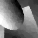
(a)	(b)	(c)	(d)

Figure 3: Additive multi-order denoising example. (a) Noisy image, (b) regularisation with $\mathop{\rm TV}\nolimits$, (c) regularisation with $\alpha_{1}\mathop{\rm TV}\nolimits+\alpha_{2}\mathop{\rm TV}\nolimits^{2}$, (d) regularisation with $\alpha_{1}\mathop{\rm TV}\nolimits+\alpha_{2}\|{\Delta\,\cdot\,}\|_{\mathcal{M}}$. All parameters are tuned to give highest PSNR with respect to the ground truth (Figure 1 (a)).

4.2 Multi-order infimal convolution

In order to overcome the smoothing effect of total variation of order two and higher, and additive combinations thereof, another idea would be to model an image $u$ as the sum of a first-order part and a second order part, i.e.,

$$u=u_{1}+u_{2}\qquad\mbox{with}\qquad u_{1}\in\mathop{\rm BV}\nolimits(\Omega),u_{2}\in\mathop{\rm BV}\nolimits^{2}(\Omega).$$

This has originally been proposed in [58], and different variants have subsequently been analysed in [16] and considered in [173, 174] in a discrete setting.

Obviously, such a decomposition exists for each $u\in\mathop{\rm BV}\nolimits(\Omega)$ but is, of course, not unique. The parts $u_{1}$ and $u_{2}$ are now regularised with first and second-order total variation associated with some weights $\alpha_{1}>0$, $\alpha_{2}>0$. The associated Tikhonov minimisation problem reads as

$$\min_{u_{1}\in\mathop{\rm BV}\nolimits(\Omega),\atop u_{2}\in\mathop{\rm BV}\nolimits^{2}(\Omega)}\ S_{f}(K(u_{1}+u_{2}))+\alpha_{1}\mathop{\rm TV}\nolimits(u_{1})+\alpha_{2}\mathop{\rm TV}\nolimits^{2}(u_{2}).$$

As we are only interested in $u$, we rewrite this problem as

$$\min_{u\in L^{p}({\Omega})}\ S_{f}(Ku)+\inf_{u_{1}\in\mathop{\rm BV}\nolimits(\Omega),\atop{u_{2}\in\mathop{\rm BV}\nolimits^{2}(\Omega),\atop u=u_{1}+u_{2}}}\ \alpha_{1}\mathop{\rm TV}\nolimits(u_{1})+\alpha_{2}\mathop{\rm TV}\nolimits^{2}(u_{2}).$$ (23)

This regularisation functional is called infimal convolution of $\alpha_{1}\mathop{\rm TV}\nolimits$ and $\alpha_{2}\mathop{\rm TV}\nolimits^{2}$.

Definition 4.6.

Let $F_{1},F_{2}:X\to{]{-\infty,\infty}]}$. Then,

$$(F_{1}\triangle F_{2})(u)=\inf_{u_{1}+u_{2}=u}\ F_{1}(u_{1})+F_{2}(u_{2})$$

is the infimal convolution of $F_{1}$ and $F_{2}$.

An infimal convolution is called exact, if for each $u\in X$ there is a pair $u_{1},u_{2}\in X$ with

$$u_{1}+u_{2}=u\qquad\mbox{and}\qquad F_{1}(u_{1})+F_{2}(u_{2})=(F_{1}\triangle F_{2})(u).$$

The infimal convolution may or may not be exact and may or may not be lower semi-continuous, even if both $F_{1}$, $F_{2}$ are lower semi-continuous. The next proposition, which should be compared to Proposition 4.1 above, provides basic properties and the function spaces associated with infimal convolutions.

Proposition 4.7.

Let ${|{\,\cdot\,}|_{1}}$ and ${|{\,\cdot\,}|_{2}}$ be two lower semi-continuous seminorms on the Banach space $X$. Then,

1. The functional ${|{\,\cdot\,}|}={|{\,\cdot\,}|_{1}}\triangle{|{\,\cdot\,}|_{2}}$ is a seminorm on $X$.

2. We have

   $$\ker({{|{\,\cdot\,}|_{1}}})+\ker({{|{\,\cdot\,}|_{2}}})\subset\ker({{|{\,\cdot\,}|}})$$

   with equality if ${|{\,\cdot\,}|_{1}}\triangle{|{\,\cdot\,}|_{2}}$ is exact.

3. If ${|{\,\cdot\,}|_{1}}\triangle{|{\,\cdot\,}|_{2}}$ is lower semi-continuous, then

   $$Y=\{{u\in X}\ \bigl{|}\ {{|{u}|}<\infty}\},\qquad\|{u}\|_{Y}=\|{u}\|_{X}+{|{u}|}$$

   constitutes a Banach space.

4. With $Y_{i}$ the Banach spaces arising from the norms $\|{\,\cdot\,}\|_{X}+{|{\,\cdot\,}|_{i}}$, $i=1,2$ (see Lemma 3.15),

   $$Y_{i}\hookrightarrow Y\quad\mbox{for }i=1,2.$$

5. It holds that $({|{\,\cdot\,}|_{1}}\triangle{|{\,\cdot\,}|_{2}})^{*}={|{\,\cdot\,}|_{1}}^{*}+{|{\,\cdot\,}|_{2}}^{*}$ and if ${|{\,\cdot\,}|_{1}}\triangle{|{\,\cdot\,}|_{2}}$ is exact, then

   $$\partial({|{\,\cdot\,}|_{1}}^{*}+{|{\,\cdot\,}|_{2}}^{*})=\partial{|{\,\cdot\,}|_{1}}^{*}+\partial{|{\,\cdot\,}|_{2}}^{*}$$

Proof.

The seminorm axioms can easily be verified for ${|{\,\cdot\,}|}$. If $u=u_{1}+u_{2}$ for $u_{i}\in\ker({{|{\,\cdot\,}|_{i}}})$, $i=1,2$, then

$${|{u}|}\leq{|{u_{1}}|_{1}}+{|{u_{2}}|_{2}}=0.$$

The converse inclusion follows directly from the exactness. The third statement is a direct consequence of Lemma 3.15 while the forth immediately follows from $\|{u}\|_{X}+{|{u}|}\leq\|{u}\|_{X}+{|{u}|_{i}}$ for $i=1,2$.

For the fifth statement, the assertion on the Fenchel dual follows by direct computation. Regarding equality of the subdifferentials, let $w\in X^{*}$ and $u\in X$ such that $u\in\partial({|{\,\cdot\,}|_{1}}^{*}+{|{\,\cdot\,}|_{2}}^{*})(w)$. Then, the Fenchel identity yields

$$\langle{w},\,{u}\rangle=({|{\,\cdot\,}|_{1}}\triangle{|{\,\cdot\,}|_{2}})(u)+{|{\,\cdot\,}|_{1}}^{*}(w)+{|{\,\cdot\,}|_{2}}^{*}(w)+={|{u_{1}}|_{1}}+{|{\,\cdot\,}|_{1}}^{*}(w)+{|{u_{2}}|_{1}}+{|{\,\cdot\,}|_{2}}^{*}(w)$$ (24)

for the minimising $u_{1},u_{2}\in X$ with $u_{1}+u_{2}=u$. As by the Fenchel inequality

$$\langle{w},\,{u_{1}}\rangle\leq{|{u_{1}}|_{1}}+{|{\,\cdot\,}|_{1}}^{*}(w)\qquad\mbox{and}\qquad\langle{w},\,{u_{2}}\rangle\leq{|{u_{2}}|_{2}}+{|{\,\cdot\,}|_{2}}^{*}(w),$$ (25)

the equation (24) can only be true when there is equality in (25). But this means, in turn, that $u_{1}\in\partial{|{\,\cdot\,}|_{1}}^{*}(w)$ and $u_{2}\in\partial{|{\,\cdot\,}|_{2}}^{*}(w)$. Hence, $\partial({|{\,\cdot\,}|_{1}}^{*}+{|{\,\cdot\,}|_{2}}^{*})\subset\partial{|{\,\cdot\,}|_{1}}^{*}+\partial{|{\,\cdot\,}|_{2}}^{*}$. The other inclusion holds trivially. ∎

The statement (v) will be relevant for obtaining optimality conditions and we note that, as can be seen from the proof, it holds true for arbitrary convex functionals, not necessarily seminorms.

The previous proposition shows in particular that lower semi-continuity and exactness of the infimal convolution are important for obtaining an appropriate function space setting. Regarding the infimal convolution of TV functionals, this holds true on $L^{p}$-spaces as follows.

Proposition 4.8.

Let $\Omega$ be a bounded Lipschitz domain, $1\leq k_{1}<k_{2}$ and $p\in{[{1,\infty}]}$ with $p\leq d/(d-k_{1})$ if $k_{1}<d$. Then, for $\alpha=(\alpha_{1},\alpha_{2})$, $\alpha_{1}>0$, $\alpha_{2}>0$, the infimal convolution

$$\mathcal{R}_{\alpha}=\alpha_{1}\mathop{\rm TV}\nolimits^{k_{1}}\triangle\alpha_{2}\mathop{\rm TV}\nolimits^{k_{2}},$$ (26)

is exact and lower semi-continuous in $L^{p}({\Omega})$.

Proof.

By continuous embedding, we may assume without loss of generality that $p<\infty$. Take a sequence $\{{u^{n}}\}$ converging to some $u$ in $L^{p}({\Omega})$ for which $\liminf_{n\to\infty}\ \mathcal{R}_{\alpha}(u^{n})<\infty$. For each $n$, we can select $u_{1}^{n},u_{2}^{n}\in\mathop{\rm BV}\nolimits^{k_{1}}(\Omega)$ such that $u^{n}=u_{1}^{n}+u_{2}^{n}$,

$$\alpha_{1}\mathop{\rm TV}\nolimits^{k_{1}}(u_{1}^{n})+\alpha_{2}\mathop{\rm TV}\nolimits^{k_{2}}(u_{2}^{n})\leq\left(\alpha_{1}\mathop{\rm TV}\nolimits^{k_{1}}\triangle\alpha_{2}\mathop{\rm TV}\nolimits^{k_{2}}\right)(u^{n})+\frac{1}{n},$$

and $u_{1}^{n}$ is in the complement of $\ker(\mathop{\rm TV}\nolimits^{k_{1}})$ in the sense that $Ru_{1}^{n}=0$ for $R:L^{p}({\Omega})\to\ker(\mathop{\rm TV}\nolimits^{k_{1}})$ a linear and continuous projection. The latter condition can always be satisfied since both $\mathop{\rm TV}\nolimits^{k_{1}}$ and $\mathop{\rm TV}\nolimits^{k_{2}}$ are invariant on $\ker(\mathop{\rm TV}\nolimits^{k_{1}})$. Now, by coercivity of $\mathop{\rm TV}\nolimits^{k_{1}}$ as in Corollary 3.23, we get that $\{{u^{n}_{1}}\}$ is bounded in $\mathop{\rm BV}\nolimits^{k_{1}}(\Omega)$. Hence, by the embedding of $\mathop{\rm BV}\nolimits^{k_{1}}(\Omega)$ in either $L^{\infty}({\Omega})$ or $L^{d/(d-k_{1})}({\Omega})$ in case of $k_{1}<d$ as in Theorem 3.20, the choice of $p$ and convergence of $\{{u^{n}}\}$ in $L^{p}({\Omega})$, we can extract (non-relabelled) subsequences of $\{{u_{1}^{n}}\}$ and $\{{u_{2}^{n}}\}$ converging weakly to some $u_{1}$ and $u_{2}$ in $L^{p}({\Omega})$, respectively, such that $u=u_{1}+u_{2}$. Thus, lower semi-continuity of both $\mathop{\rm TV}\nolimits^{k_{1}}$ and $\mathop{\rm TV}\nolimits^{k_{2}}$ implies

$$\left(\alpha_{1}\mathop{\rm TV}\nolimits^{k_{1}}\triangle\alpha_{2}\mathop{\rm TV}\nolimits^{k_{2}}\right)(u) \leq\alpha_{1}\mathop{\rm TV}\nolimits^{k_{1}}(u_{1})+\alpha_{2}\mathop{\rm TV}\nolimits^{k_{2}}(u_{2})$$

$$\leq\liminf_{n\to\infty}\ \left(\alpha_{1}\mathop{\rm TV}\nolimits^{k_{1}}(u^{n}_{1})+\alpha_{2}\mathop{\rm TV}\nolimits^{k_{2}}(u^{n}_{2})\right)$$

$$=\liminf_{n\to\infty}\ \left(\alpha_{1}\mathop{\rm TV}\nolimits^{k_{1}}\triangle\alpha_{2}\mathop{\rm TV}\nolimits^{k_{2}}\right)(u^{n})$$

such that lower semi-continuity holds. Finally, exactness for $u\in L^{p}({\Omega})$ with $\mathcal{R}_{\alpha}(u)<\infty$ follows from choosing $\{{u^{n}}\}$ as the sequence that is constant $u$. ∎

Given this, the special case ${|{\,\cdot\,}|_{i}}=\alpha_{i}\mathop{\rm TV}\nolimits^{k_{i}}$ and $X=L^{1}({\Omega})$ of Proposition 4.7 shows that both $\mathop{\rm BV}\nolimits^{k_{1}}(\Omega)$ and $\mathop{\rm BV}\nolimits^{k_{2}}(\Omega)$ are embedded in the Banach space $Y$. Hence, in contrast to the sum of different TV terms, their infimal convolution allows to recover jumps whenever $k_{1}=1$, independent of $k_{2}$. In fact, as the following proposition shows, the space $Y$ is even equivalent to the BV space corresponding to the lowest order, in particular to $\mathop{\rm BV}\nolimits(\Omega)$ for $k_{1}=1$. Again, the result should be compared to Theorem 4.2 above.

Theorem 4.9.

Let $1\leq k_{1}<k_{2}$, $\alpha_{1}>0$, $\alpha_{2}>0$, $\Omega$ be a bounded Lipschitz domain, and $Y$ be the Banach space associated with $X=L^{1}({\Omega})$ and total-variation infimal convolution according to (26). Then,

$$Y=\mathop{\rm BV}\nolimits^{k_{1}}(\Omega)$$

in the sense of Banach space equivalence, and for $p\in[1,\infty]$, $p\leq d/(d-k_{1})$ if $k_{1}<d$, and for $R:L^{p}({\Omega})\to\ker({\mathop{\rm TV}\nolimits^{k_{2}}})$ a linear, continuous projection there exists a $C>0$ such that

$$\|{u-Ru}\|_{p}\leq C\min\{{\alpha_{1},\alpha_{2}}\}^{-1}(\alpha_{1}\mathop{\rm TV}\nolimits^{k_{1}}\triangle\alpha_{2}\mathop{\rm TV}\nolimits^{k_{2}})(u)$$ (27)

for all $u\in L^{p}({\Omega})$.

Proof.

We first show the claimed norm equivalence. For this purpose, note that one estimate corresponds to the fourth statement in Proposition 4.7. For the converse estimate, let $u\in\mathop{\rm BV}\nolimits^{k_{1}}(\Omega)$ and $R:L^{1}({\Omega})\to\ker({\mathop{\rm TV}\nolimits^{k_{2}}})$ be a projection. Then,

$$\mathop{\rm TV}\nolimits^{k_{1}}(u)\leq C\bigl{(}\|{u}\|_{1}+\mathop{\rm TV}\nolimits^{k_{1}}(u-Rw)\bigr{)}$$ (28)

for $C$ independent of $u,w\in\mathop{\rm BV}\nolimits^{k_{1}}(\Omega)$. Indeed, if for $\{{u^{n}}\}$ and $\{{w^{n}}\}$ we have $\mathop{\rm TV}\nolimits^{k_{1}}(u^{n})=1$ and $\|{u^{n}}\|_{1}\to 0$ as well as $\mathop{\rm TV}\nolimits^{k_{1}}(u^{n}-Rw^{n})\to 0$, meaning $u^{n}\to 0$ in $L^{1}({\Omega})$ and $\nabla^{k_{1}}(u^{n}-Rw^{n})\to 0$ in $\mathcal{M}({\Omega,\mathop{\rm Sym}\nolimits^{k_{1}}(\mathbf{R}^{d})})$. The latter implies that $\{{\nabla^{k_{1}}Rw^{n}}\}$ is bounded in a finite-dimensional space, hence there is a convergent subsequence (not relabelled) with limit $v\in\mathcal{M}({\Omega,\mathop{\rm Sym}\nolimits^{k_{1}}(\mathbf{R}^{d})})$. Then, $\nabla^{k_{1}}u^{n}\to v$ in $\mathcal{M}({\Omega,\mathop{\rm Sym}\nolimits^{k_{1}}(\mathbf{R}^{d})})$ and the closedness of $\nabla^{k_{1}}$ yields $v=0$ which is a contradiction to $\mathop{\rm TV}\nolimits^{k_{1}}(u^{n})=1$ for all $n$.

Using this, together with the estimate

$$\mathop{\rm TV}\nolimits^{k_{1}}(w-Rw)\leq C\mathop{\rm TV}\nolimits^{k_{2}}(w)$$ (29)

from Lemma 3.25, it holds for $u\in\mathop{\rm BV}\nolimits^{k_{1}}(\Omega)$ and $w\in\mathop{\rm BV}\nolimits^{k_{2}}(\Omega)$ that

$$\mathop{\rm TV}\nolimits^{k_{1}}(u) \leq C\bigl{(}\|{u}\|_{1}+\mathop{\rm TV}\nolimits^{k_{1}}(u-Rw)\bigr{)}$$

$$\leq C\bigl{(}\|{u}\|_{1}+\mathop{\rm TV}\nolimits^{k_{1}}(u-w)+\mathop{\rm TV}\nolimits^{k_{1}}(w-Rw)\bigr{)}$$

$$\leq C\bigl{(}\|{u}\|_{1}+\mathop{\rm TV}\nolimits^{k_{1}}(u-w)+\mathop{\rm TV}\nolimits^{k_{2}}(w)\bigr{)}.$$

Taking the infimum over all $w\in\mathop{\rm BV}\nolimits^{k_{2}}(\Omega)$, adding $\|{u}\|_{1}$ on both sides as well as observing that $\mathop{\rm TV}\nolimits^{k_{1}}\triangle\mathop{\rm TV}\nolimits^{k_{2}}\leq\min\{{\alpha_{1},\alpha_{2}}\}^{-1}(\alpha_{1}\mathop{\rm TV}\nolimits^{k_{1}}\triangle\alpha_{2}\mathop{\rm TV}\nolimits^{k_{2}})$ yields

$$\|{u}\|_{1}+\mathop{\rm TV}\nolimits^{k_{1}}(u)\leq C\bigl{(}\|{u}\|_{1}+\min\{{\alpha_{1},\alpha_{2}}\}^{-1}(\alpha_{1}\mathop{\rm TV}\nolimits^{k_{1}}\triangle\alpha_{2}\mathop{\rm TV}\nolimits^{k_{2}})(u)\bigr{)},$$

and, consequently, the desired norm estimate. Likewise, the estimate $\|u-Ru\|_{p}\leq C(\mathop{\rm TV}\nolimits^{k_{1}}\triangle\mathop{\rm TV}\nolimits^{k_{2}})(u)$ follows in analogy to Proposition 3.22 and Corollary 3.23, which immediately gives the claimed estimate for arbitrary $\alpha_{1}>0$, $\alpha_{2}>0$. ∎

Tikhonov regularisation.

Again, the second estimate in Theorem 4.9 is crucial as it allows to apply the well-posedness result of Theorem 3.26.

Proposition 4.10.

With $X=L^{p}(\Omega)$, $p\in{]{1,\infty}[}$, $\Omega$ being a bounded Lipschitz domain, $Y$ a Banach space, $K:X\to Y$ linear and continuous, $S_{f}:Y\to[0,\infty]$ proper, convex lower semi-continuous and coercive, $1\leq k_{1}<k_{2}$, $\alpha_{1}>0$, $\alpha_{2}>0$, the Tikhonov minimisation problem

$$\min_{u\in L^{p}({\Omega})}\ S_{f}(Ku)+\left(\alpha_{1}\mathop{\rm TV}\nolimits^{k_{1}}\triangle\alpha_{2}\mathop{\rm TV}\nolimits^{k_{2}}\right)(u).$$ (30)

is well-posed in the sense of Theorem 3.26 whenever $p\leq d/(d-k_{1})$ if $k_{1}<d$.

Compared to the sum of different TV terms, we see that now the necessary coercivity estimate incorporates a projection to the larger kernel of $\mathop{\rm TV}\nolimits^{k_{2}}$ and an $L^{p}$ norm with a smaller exponent corresponding to $\mathop{\rm TV}\nolimits^{k_{1}}$. Hence, in view of the assumptions of Theorem 3.26, the infimal convolution of $\mathop{\rm TV}\nolimits^{k_{1}}$ and $\mathop{\rm TV}\nolimits^{k_{2}}$ inherits the worst properties of the two summands, i.e., the ones that are more restrictive for applications in an inverse problems context. Nevertheless, such a slightly more restrictive assumption on the continuity of the forward operator is compensated by the fact that the infimal convolution with $k_{1}=1$ allows to reconstruct jumps. In addition, each solution $u^{*}$ of a Tikhonov functional admits an optimal decomposition $u^{*}=u_{1}^{*}+u_{2}^{*}$ with $u_{i}^{*}\in\mathop{\rm BV}\nolimits^{k_{i}}(\Omega)$, $i=1,2$, which follows from the exactness of the infimal convolution.

Regarding the convergence result of Theorem 3.28 and the rates of Proposition 3.29, again a direct extension to regularisation with $\alpha_{1}\mathop{\rm TV}\nolimits^{k_{1}}\triangle\alpha_{2}\mathop{\rm TV}\nolimits^{k_{2}}$ can be obtained by regarding the weights $\alpha_{1},\alpha_{2}$ to be fixed and introducing a additional factor $\alpha>0$ for both terms, which then acts as the regularisation parameter. Considering the limiting behaviour for both weights converging to zero, a counterpart of Theorem 4.4 can be obtained as follows. There, we allow also for infinite weights $\alpha_{i}$, i.e., for $\alpha_{i}=\infty$, we set $\alpha_{i}\mathop{\rm TV}\nolimits^{k_{i}}(u)=0$ if $u\in{\ker(\mathop{\rm TV}\nolimits^{k_{i}})}$ and $\alpha_{i}\mathop{\rm TV}\nolimits^{k_{i}}(u)=\infty$ else. We first need a lower semi-continuity result.

Lemma 4.11.

Let $\Omega$ be a bounded Lipschitz domain, $p\in{[{1,\infty}[}$ with $1\leq p\leq d/(d-k_{1})$ if $k_{1}<d$, $\{{(\alpha_{1,n},\alpha_{2,n})}\}$ be a sequence of positive parameters converging to some $(\alpha^{\dagger}_{1},\alpha_{2}^{\dagger})\in{]{0,\infty}]}^{2}$ and $\{{u^{n}}\}$ be a sequence in $L^{p}(\Omega)$ weakly converging to $u^{*}\in L^{p}(\Omega)$. Then,

$$\left(\alpha_{1}^{\dagger}\mathop{\rm TV}\nolimits^{k_{1}}\triangle\alpha_{2}^{\dagger}\mathop{\rm TV}\nolimits^{k_{2}}\right)(u^{*})\leq\liminf_{n\rightarrow\infty}\ \left(\alpha_{1,n}\mathop{\rm TV}\nolimits^{k_{1}}\triangle\alpha_{2,n}\mathop{\rm TV}\nolimits^{k_{2}}\right)(u^{n}).$$

Proof.

By moving to a subsequence, we can assume that $\left(\alpha_{1,n}\mathop{\rm TV}\nolimits^{k_{1}}\triangle\alpha_{2,n}\mathop{\rm TV}\nolimits^{k_{2}}\right)(u^{n})$ converges to the limes inferior on the right-hand side of the claimed assertion and that the latter is finite. Choose $\{{u_{1}^{n}}\}$, $\{{u_{2}^{n}}\}$ sequences such that for each $n$, we have $u_{1}^{n}+u_{2}^{n}=u^{n}$, $\left(\alpha_{1,n}\mathop{\rm TV}\nolimits^{k_{1}}\triangle\alpha_{2,n}\mathop{\rm TV}\nolimits^{k_{2}}\right)(u^{n})=\alpha_{1,n}\mathop{\rm TV}\nolimits^{k_{1}}(u_{1}^{n})+\alpha_{2,n}\mathop{\rm TV}\nolimits^{k_{2}}(u_{2}^{n})$ and $u_{1}^{n}$ being in a complement of $\ker(\mathop{\rm TV}\nolimits^{k_{1}})$ in the sense that $u_{1}^{n}\in\ker({R})$ for a linear, continuous projection $R:L^{p}({\Omega})\to\ker({\mathop{\rm TV}\nolimits^{k_{1}}})$. Setting $\hat{\alpha}_{i}=\inf\ \{\alpha_{i,n}\}>0$, we obtain

$$\hat{\alpha}_{1}\mathop{\rm TV}\nolimits^{k_{1}}(u_{1}^{n})+\hat{\alpha}_{2}\mathop{\rm TV}\nolimits^{k_{2}}(u_{2}^{n})\leq\alpha_{1,n}\mathop{\rm TV}\nolimits^{k_{1}}(u_{1}^{n})+\alpha_{2,n}\mathop{\rm TV}\nolimits^{k_{2}}(u_{2}^{n}).$$

In particular, for a constant $C>0$ it holds that

$$\|{u_{1}^{n}}\|_{p}\leq C\hat{\alpha}_{1}\mathop{\rm TV}\nolimits^{k_{1}}(u_{1}^{n})\leq C(\alpha_{1,n}\mathop{\rm TV}\nolimits^{k_{1}}(u_{1}^{n})+\alpha_{2,n}\mathop{\rm TV}\nolimits^{k_{2}}(u_{2}^{n})),$$

which implies that $\{{u_{1}^{n}}\}$ is bounded in $\mathop{\rm BV}\nolimits^{k_{1}}(\Omega)$. By the embedding of Theorem 3.20 and since $\{{u^{n}}\}$ is convergent, both $\{{u_{1}^{n}}\}$ and $\{{u_{2}^{n}}\}$ admit subsequences (not relabelled) weakly converging to some $u_{1}^{*}$ and $u_{2}^{*}$ in $L^{p}(\Omega)$, respectively. Now, in case $\alpha_{i}^{\dagger}<\infty$, we can conclude

$$\alpha_{i}^{\dagger}\mathop{\rm TV}\nolimits^{k_{i}}(u_{i}^{*})\leq\liminf_{n\to\infty}\ \alpha_{i,n}\mathop{\rm TV}\nolimits^{k_{i}}(u_{i}^{n}).$$

Otherwise, we get by boundedness of $\alpha_{i,n}\mathop{\rm TV}\nolimits^{k_{i}}(u_{i}^{n})$ that $\mathop{\rm TV}\nolimits^{k_{i}}(u_{i}^{n})\rightarrow 0$ and by lower semi-continuity that $\mathop{\rm TV}\nolimits^{k_{i}}(u^{*}_{i})=0$. Together, this implies

$$\left(\alpha_{1}^{\dagger}\mathop{\rm TV}\nolimits^{k_{1}}\triangle\alpha_{2}^{\dagger}\mathop{\rm TV}\nolimits^{k_{2}}\right)(u^{*})\leq\alpha_{1}^{\dagger}\mathop{\rm TV}\nolimits^{k_{1}}(u_{1}^{*})+\alpha_{2}^{\dagger}\mathop{\rm TV}\nolimits^{k_{2}}(u_{2}^{*})$$

$$\leq\liminf_{n\to\infty}\ \left(\alpha_{1,n}\mathop{\rm TV}\nolimits^{k_{1}}(u_{1}^{n})+\alpha_{2,n}\mathop{\rm TV}\nolimits^{k_{2}}(u_{2}^{n})\right)$$

$$=\liminf_{n\to\infty}\ \left(\alpha_{1,n}\mathop{\rm TV}\nolimits^{k_{1}}\triangle\alpha_{2,n}\mathop{\rm TV}\nolimits^{k_{2}}\right)(u^{n}).$$

This implies the desired statement. ∎

Theorem 4.12.

In the situation of Proposition 4.10 and for $p\in{]{1,\infty}[}$ with $p\leq d/(d-k_{1})$ in case of $k_{1}<d$, let for each $\delta>0$ the data $f^{\delta}$ be given such that $S_{f^{\delta}}(f^{\dagger})\leq\delta$, let $\{{S_{f^{\delta}}}\}$ be equi-coercive and converge to $S_{f^{\dagger}}$ for some data $f^{\dagger}$ in $Y$ in the sense of (4) and $S_{f^{\dagger}}(v)=0$ if and only if $v=f^{\dagger}$.

Choose the parameters $\alpha=(\alpha_{1},\alpha_{2})$ in dependence of $\delta$ such that

$$\min\{\alpha_{1},\alpha_{2}\}\to 0,\quad\frac{\delta}{\min\{\alpha_{1},\alpha_{2}\}}\to 0,\qquad\mbox{as}\qquad\delta\to 0,$$

and assume that $(\tilde{\alpha}_{1},\tilde{\alpha}_{2})=(\alpha_{1},\alpha_{2})/\min\{\alpha_{1},\alpha_{2}\}\rightarrow(\alpha_{1}^{\dagger},\alpha_{2}^{\dagger})\in{]{0,\infty}]}^{2}$ as $\delta\to 0$. Set

$$k=\left\{\begin{array}[]{rl}k_{1}&\mbox{if}\ \alpha_{1}^{\dagger}<\infty,\\ k_{2}&\mbox{else},\end{array}\right.$$

and assume that there exists $u_{0}\in\mathop{\rm BV}\nolimits^{k}(\Omega)$ such that $Ku_{0}=f^{\dagger}$.

Then, up to shifts in $\ker({K})\cap\mathbf{P}^{k_{2}-1}$, any sequence $\{{u^{\alpha,\delta}}\}$, with each $u^{\alpha,\delta}$ being a solution to (30) for parameters $(\alpha_{1},\alpha_{2})$ and data $f^{\delta}$, has at least one $L^{p}$-weak accumulation point. Each $L^{p}$-weak accumulation point is a minimum-$(\alpha_{1}^{\dagger}\mathop{\rm TV}\nolimits^{k_{1}}\triangle\alpha_{2}^{\dagger}\mathop{\rm TV}\nolimits^{k_{2}})$-solution of $Ku=f^{\dagger}$ and $\lim_{\delta\to 0}(\tilde{\alpha}_{1}\mathop{\rm TV}\nolimits^{k_{1}}\triangle\tilde{\alpha}_{2}\mathop{\rm TV}\nolimits^{k_{2}})(u^{\alpha,\delta})=(\alpha_{1}^{\dagger}\mathop{\rm TV}\nolimits^{k_{1}}\triangle\alpha_{2}^{\dagger}\mathop{\rm TV}\nolimits^{k_{2}})(u^{\dagger})$.

Proof.

First note that, with $R:L^{p}(\Omega)\rightarrow\ker(\mathop{\rm TV}\nolimits^{k_{2}})$ a linear, continuous projection, for any $u\in L^{p}(\Omega)$, we have

$$\|u-Ru\|_{p}\leq C(\mathop{\rm TV}\nolimits^{k_{1}}\triangle\mathop{\rm TV}\nolimits^{k_{2}})(u)\leq C(\alpha^{\dagger}_{1}\mathop{\rm TV}\nolimits^{k_{1}}\triangle\alpha^{\dagger}_{2}\mathop{\rm TV}\nolimits^{k_{2}})(u),$$

and by the choice of $k$ as well as $u_{0}\in\mathop{\rm BV}\nolimits^{k}(\Omega)$, that $(\alpha_{1}^{\dagger}\mathop{\rm TV}\nolimits^{k_{1}}\triangle\alpha_{2}^{\dagger}\mathop{\rm TV}\nolimits^{k_{2}})(u_{0})<\infty$. Hence, as a consequence of Theorem 3.26, there exists a minimum-$(\alpha_{1}^{\dagger}\mathop{\rm TV}\nolimits^{k_{1}}\triangle\alpha_{2}^{\dagger}\mathop{\rm TV}\nolimits^{k_{2}})$-solution $u^{\dagger}\in\mathop{\rm BV}\nolimits^{k}(\Omega)$ to $Ku=f^{\dagger}$. Using optimality of $u^{\alpha,\delta}$ compared to $u^{\dagger}$ gives

$$S_{f^{\delta}}(Ku^{\alpha,\delta})+\left(\alpha_{1}\mathop{\rm TV}\nolimits^{k_{1}}\triangle\alpha_{2}\mathop{\rm TV}\nolimits^{k_{2}}\right)(u^{\alpha,\delta})\leq\delta+\left(\alpha_{1}\mathop{\rm TV}\nolimits^{k_{1}}\triangle\alpha_{2}\mathop{\rm TV}\nolimits^{k_{2}}\right)(u^{\dagger}).$$

Now since $\left(\alpha_{1}\mathop{\rm TV}\nolimits^{k_{1}}\triangle\alpha_{2}\mathop{\rm TV}\nolimits^{k_{2}}\right)(u^{\dagger})\leq\min_{i=1,2}\{\alpha_{i}\mathop{\rm TV}\nolimits^{k_{i}}(u^{\dagger})\}$ and $\min\{\alpha_{1},\alpha_{2}\}\to 0$ as $\delta\rightarrow 0$, we have that $S_{f^{\delta}}(Ku^{\alpha,\delta})\to 0$ as $\delta\to 0$. Moreover, as also $\delta/\min\{\alpha_{1},\alpha_{2}\}\to 0$, it follows that

$$\limsup_{\delta\rightarrow 0}\ \left(\tilde{\alpha}_{1}\mathop{\rm TV}\nolimits^{k_{1}}\triangle\tilde{\alpha}_{2}\mathop{\rm TV}\nolimits^{k_{2}}\right)(u^{\alpha,\delta}) \leq\limsup_{\delta\rightarrow 0}\ \left(\tilde{\alpha}_{1}\mathop{\rm TV}\nolimits^{k_{1}}\triangle\tilde{\alpha}_{2}\mathop{\rm TV}\nolimits^{k_{2}}\right)(u^{\dagger})$$

$$\leq(1+\varepsilon)\left(\alpha_{1}^{\dagger}\mathop{\rm TV}\nolimits^{k_{1}}\triangle\alpha_{2}^{\dagger}\mathop{\rm TV}\nolimits^{k_{2}}\right)(u^{\dagger})$$

for $\varepsilon>0$ independent of $u^{\alpha,\delta}$ and letting $\epsilon\rightarrow 0$, we obtain

$$\limsup_{\delta\rightarrow 0}\left(\tilde{\alpha}_{1}\mathop{\rm TV}\nolimits^{k_{1}}\triangle\tilde{\alpha}_{2}\mathop{\rm TV}\nolimits^{k_{2}}\right)(u^{\alpha,\delta})\leq\left(\alpha_{1}^{\dagger}\mathop{\rm TV}\nolimits^{k_{1}}\triangle\alpha_{2}^{\dagger}\mathop{\rm TV}\nolimits^{k_{2}}\right)(u^{\dagger}).$$

In particular, using (27), we can conclude that $\{{u^{\alpha,\delta}-Ru^{\alpha,\delta}}\}$ is bounded in $L^{p}({\Omega})$. By introducing appropriate shifts in $\ker({K})\cap\mathbf{P}^{k_{2}-1}$ as done in Theorem 3.26 and using the equi-coercivity of $\{{S_{f^{\delta}}}\}$, one can then achieve that $\{{u^{\alpha,\delta}}\}$ is bounded in $L^{p}({\Omega})$ such that by reflexivity, it admits a $L^{p}$-weak accumulation point.

Next, let $u^{*}$ be a $L^{p}$-weak accumulation point associated with $\{{\delta_{n}}\}$, $\delta_{n}\to 0$ as well as the corresponding parameters $\{{\alpha_{n}}\}=\{{(\alpha_{1,n},\alpha_{2,n})}\}$. Then, $S_{f^{\dagger}}(Ku^{*})\leq\liminf_{n\to\infty}\ S_{f^{\delta_{n}}}(Ku^{\alpha_{n},\delta_{n}})=0$ by convergence of $S_{f^{\delta}}$ to $S_{f^{\dagger}}$, so $Ku^{*}=f^{\dagger}$. Moreover, employing Lemma 4.11, we get

$$\left(\alpha_{1}^{\dagger}\mathop{\rm TV}\nolimits^{k_{1}}\triangle\alpha_{2}^{\dagger}\mathop{\rm TV}\nolimits^{k_{2}}\right)(u^{*}) \leq\liminf_{n\to\infty}\ \left(\tilde{\alpha}_{1,n}\mathop{\rm TV}\nolimits^{k_{1}}\triangle\tilde{\alpha}_{2,n}\mathop{\rm TV}\nolimits^{k_{2}}\right)(u^{\alpha_{n},\delta_{n}})$$

$$\leq\left(\alpha_{1}^{\dagger}\mathop{\rm TV}\nolimits^{k_{1}}\triangle\alpha_{2}^{\dagger}\mathop{\rm TV}\nolimits^{k_{2}}\right)(u^{\dagger}),$$

hence, $u^{*}$ is a minimum-$\left(\alpha_{1}^{\dagger}\mathop{\rm TV}\nolimits^{k_{1}}\triangle\alpha_{2}^{\dagger}\mathop{\rm TV}\nolimits^{k_{2}}\right)(u^{\dagger})$-solution. The remaining assertions follow as in the proof of Theorem 4.4 by replacing the sum with the infimal convolution. ∎

Remark 4.13.

• It is also possible to construct infimal convolutions of more than two $\mathop{\rm TV}\nolimits$-type functionals and, of course, other functionals than $\mathop{\rm TV}\nolimits^{k}$.

• Introducing orders $k_{1},\ldots,k_{m}\geq 1$ and weights $\alpha_{1},\ldots,\alpha_{m}>0$, one can consider

  $$\min_{u\in L^{p}({\Omega})}S_{f}(Ku)+\Bigl{(}\bigtriangleup_{i=1}^{m}\alpha_{i}\mathop{\rm TV}\nolimits^{k_{i}}\Bigr{)}(u).$$ (31)

  Solutions then exist, for appropriate $p$, in the space $\mathop{\rm BV}\nolimits^{k}(\Omega)$ for $k=\min\{{k_{1},\ldots,k_{m}}\}$.

• The latter is in contrast to the multi-order $\mathop{\rm TV}\nolimits$ regularisation (20) where the solution space is determined by the highest effective order of differentiation. Letting $k_{i}=1$ for some $i$, the solution space is then $\mathop{\rm BV}\nolimits(\Omega)$ which allows for discontinuities; a desirable property for image restoration.

Optimality conditions.

Again, in the situation that $Y$ is a Hilbert space, $q=2$ and $S_{f}(v)=\frac{1}{2}\|{v-f}\|_{Y}^{2}$, we obtain some first-order optimality conditions. Noting that the dual of the infimal convolution of two functions is the sum of the respective duals, and arguing according to Proposition 3.30, an $u^{*}$ is optimal for (30) if and only if

$$u^{*}\in\partial\bigl{(}(\alpha_{1}\mathop{\rm TV}\nolimits^{k_{1}})^{*}+(\alpha_{2}\mathop{\rm TV}\nolimits^{k_{2}})^{*}\bigr{)}\bigl{(}K^{*}(f-Ku^{*})\bigr{)}.$$

By Proposition 4.7, the subgradients are additive, so in terms of the normal cones introduced in Proposition 3.30, the optimality condition reads as

$$u^{*}\in\mathcal{N}_{\mathop{\rm TV}\nolimits^{k_{1}}}\Bigl{(}\frac{K^{*}(f-Ku^{*})}{\alpha_{1}}\Bigr{)}+\mathcal{N}_{\mathop{\rm TV}\nolimits^{k_{2}}}\Bigl{(}\frac{K^{*}(f-Ku^{*})}{\alpha_{2}}\Bigr{)}.$$ (32)

A-priori estimates.

Also here, in the above Hilbert space situation, i.e., $S_{f}(v)=\frac{1}{2}\|{v-f}\|_{Y}^{2}$ and $Y$ Hilbert space, an a-priori bound of solutions $u^{*}$ can be derived thanks to the coercivity estimate (27). One indeed has $\|{u-Ru}\|_{p}\leq\frac{1}{2\min\{{\alpha_{1},\alpha_{2}}\}}C\|{f}\|_{Y}^{2}$ with $R$ and $C$ coming from (27). Hence, assuming that $K$ is injective on $\mathbf{P}^{k_{2}-1}$, which leads to $c\|{Ru}\|_{p}\leq\|{KRu}\|_{Y}$ for all $u$ and some $c>0$, one proceeds analogously to Remark 3.31 to obtain the bound (17) with $\alpha$ replaced by $\min\{{\alpha_{1},\alpha_{2}}\}$. By analogy, for $S_{f}(v)=\mathop{\rm KL}\nolimits(v,f)$ being the Kullback–Leibler discrepancy, an a-priori estimate of the type (18) follows.

Moreover, it is possible to control $w^{*}$ up to $\mathbf{P}^{k_{1}-1}$ whenever $(\alpha_{1}\mathop{\rm TV}\nolimits^{k_{1}}\triangle\alpha_{2}\mathop{\rm TV}\nolimits^{k_{2}})(u^{*})=\alpha_{1}\mathop{\rm TV}\nolimits^{k_{1}}(u^{*}-w^{*})+\alpha_{2}\mathop{\rm TV}\nolimits^{k_{2}}(w^{*})$. Let, in the following, $C_{f}\geq 0$ be an a-priori estimate for the optimal functional value, for instance, $C_{f}=\frac{1}{2}\|{f}\|_{Y}^{2}$ in case of $S_{f}(v)=\frac{1}{2}\|{v-f}\|_{Y}^{2}$, and $C_{f}=\mathop{\rm KL}\nolimits(Ku^{0},f)+(\alpha_{1}\mathop{\rm TV}\nolimits^{k_{1}}\triangle\alpha_{2}\mathop{\rm TV}\nolimits^{k_{2}})(u^{0})$ for a $u^{0}\in\mathop{\rm BV}\nolimits^{k_{1}}(\Omega)$ with $\mathop{\rm KL}\nolimits(Ku^{0},f)<\infty$ in case of $S_{f}(v)=\mathop{\rm KL}\nolimits(v,f)$. Further, denoting by $\tilde{C}>0$ a constant such that $\mathop{\rm TV}\nolimits^{k_{1}}(u)\leq\tilde{C}\bigl{(}\|{u}\|_{1}+\min\{{\alpha_{1},\alpha_{2}}\}^{-1}(\alpha_{1}\mathop{\rm TV}\nolimits^{k_{1}}\triangle\alpha_{2}\mathop{\rm TV}\nolimits^{k_{2}})(u)\bigr{)}$ for all $u\in\mathop{\rm BV}\nolimits^{k_{1}}(u)$ (which exists by virtue of the norm equivalence in Theorem 4.9), we see that $\mathop{\rm TV}\nolimits^{k_{1}}(u^{*})\leq\tilde{C}\bigl{(}{|{\Omega}|}^{1/p}\|{u^{*}}\|_{p}+\min\{{\alpha_{1},\alpha_{2}}\}^{-1}C_{f}\bigr{)}$, hence

$$\alpha_{1}\mathop{\rm TV}\nolimits^{k_{1}}(w^{*})\leq\alpha_{1}\mathop{\rm TV}\nolimits^{k_{1}}(u^{*}-w^{*})+\alpha_{1}\mathop{\rm TV}\nolimits^{k_{1}}(u^{*})+\alpha_{2}\mathop{\rm TV}\nolimits^{k_{2}}(w^{*})\leq\alpha_{1}\mathop{\rm TV}\nolimits^{k_{1}}(u^{*})+C_{f}.$$

Consequently, we obtain the bound

$$\mathop{\rm TV}\nolimits^{k_{1}}(w^{*})\leq\tilde{C}{|{\Omega}|}^{1/p}\|{u^{*}}\|_{p}+\frac{(\tilde{C}+1)C_{f}}{\min\{{\alpha_{1},\alpha_{2}}\}},$$ (33)

which gives an a-priori estimate when plugging in the already-obtained bound on $\|{u^{*}}\|_{p}$. Moreover, this estimate implies a bound on $\|{w^{*}-Rw^{*}}\|_{p}$ by the Poincaré–Wirtinger inequality. However, the norm of $w^{*}$ can not fully be controlled since adding an element in $\mathbf{P}^{k_{1}-1}=\ker(\mathop{\rm TV}\nolimits^{k_{1}})$ to $w^{*}$ would still realise the infimum in the infimal convolution. Thus, an estimate of the type (33) is the best one could except in the considered setting.

Denoising performance.

Figure 4 shows that it is indeed beneficial for denoising to regularise with $\alpha_{1}\mathop{\rm TV}\nolimits\triangle\alpha_{2}\mathop{\rm TV}\nolimits^{2}$ compared to pure $\mathop{\rm TV}\nolimits$-regularisation: Higher-order features as well as edges are recognised by this image model. Nevertheless, staircase artefacts are still present, see Figure 4 (c). Essentially, this does not change when the second-order component of the infimal convolution is replaced, for instance by $\|{\Delta\,\cdot\,}\|_{\mathcal{M}}$ as in Remark 3.33, see Figure 4 (d). (For the latter penalty functional, basically the same problems as the ones mentioned in Remark 3.33 appear.)

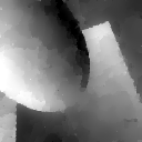
(a)	(b)	(c)	(d)

Figure 4: Infimal-convolution denoising example. (a) Noisy image, (b) regularisation with $\mathop{\rm TV}\nolimits$, (c) regularisation with $\alpha_{1}\mathop{\rm TV}\nolimits\triangle\alpha_{2}\mathop{\rm TV}\nolimits^{2}$, (d) regularisation with $\alpha_{1}\mathop{\rm TV}\nolimits\triangle\alpha_{2}\|{\Delta\,\cdot\,}\|_{\mathcal{M}}$. All parameters are tuned to give highest PSNR with respect to the ground truth (Figure 1 (a)).

5 Total generalised variation (TGV)

5.1 Basic concepts

As a motivation for TGV, consider the formal predual ball associated with the infimal convolution $\mathcal{R}_{\alpha}=\alpha_{1}\mathop{\rm TV}\nolimits\triangle\alpha_{0}\mathop{\rm TV}\nolimits^{2}$ for $\alpha=(\alpha_{0},\alpha_{1})$, $\alpha_{0},\alpha_{1}>0$. Then

$$\mathcal{R}^{*}_{\alpha}=(\alpha_{1}\mathop{\rm TV}\nolimits)^{*}+(\alpha_{0}\mathop{\rm TV}\nolimits^{2})^{*}=\mathcal{I}_{\overline{\mathcal{B}}}\qquad\mbox{with}\qquad\overline{\mathcal{B}}=\alpha_{1}\overline{\mathcal{B}_{\mathop{\rm TV}\nolimits}}\cap\alpha_{0}\overline{\mathcal{B}_{\mathop{\rm TV}\nolimits^{2}}}$$

and

$$\alpha_{1}\mathcal{B}_{\mathop{\rm TV}\nolimits} =\{{\mathop{\rm div}\nolimits\varphi_{1}}\ \bigl{|}\ {\varphi_{1}\in\mathcal{C}_{\mathrm{c}}^{1}({\Omega,\mathbf{R}^{d}}),\ \|{\varphi_{1}}\|_{\infty}\leq\alpha_{1}}\},$$

$$\alpha_{0}\mathcal{B}_{\mathop{\rm TV}\nolimits^{2}} =\{{\mathop{\rm div}\nolimits^{2}\varphi_{2}}\ \bigl{|}\ {\varphi_{2}\in\mathcal{C}_{\mathrm{c}}^{2}({\Omega,\mathop{\rm Sym}\nolimits^{2}(\mathbf{R}^{d})}),\ \|{\varphi_{2}}\|_{\infty}\leq\alpha_{0}}\}.$$

Neglecting the closure for a moment, this leads to the predual ball according to

$$\mathcal{B}=\{{\varphi}\ \bigl{|}\ {\varphi=\mathop{\rm div}\nolimits\varphi_{1}=\mathop{\rm div}\nolimits^{2}\varphi_{2},\ \varphi_{i}\in\mathcal{C}_{\mathrm{c}}^{i}({\Omega,\mathop{\rm Sym}\nolimits^{i}(\mathbf{R}^{d})}),\ \|{\varphi_{i}}\|_{\infty}\leq\alpha_{2-i},\ i=1,2}\}.$$ (34)

Each $\varphi\in\mathcal{B}$ possesses a representation as an $\infty$-bounded first and second-order divergence of some $\varphi_{1}$ and $\varphi_{2}$. However, as the kernel of the divergence is non-trivial (and even infinite-dimensional for $d\geq 2$), we can only conclude that $\varphi_{1}=\mathop{\rm div}\nolimits\varphi_{2}+\eta$ for some $\eta$ with $\mathop{\rm div}\nolimits\eta=0$. Enforcing $\eta=0$ thus gives the set

$$\mathcal{B}_{\mathop{\rm TGV}\nolimits^{2}_{\alpha}}=\{{\mathop{\rm div}\nolimits^{2}\varphi}\ \bigl{|}\ {\varphi\in\mathcal{C}_{\mathrm{c}}^{2}({\Omega,\mathop{\rm Sym}\nolimits^{2}(\mathbf{R}^{d})}),\ \|{\mathop{\rm div}\nolimits^{m}\varphi}\|_{\infty}\leq\alpha_{m},\ m=0,1}\}$$

which leads, interpreted as a predual ball, to a seminorm which also incorporates first- and second-order derivatives but is different from infimal convolution: the total generalised variation [37].

There is also a primal version of this motivation via the $(\mathop{\rm TV}\nolimits$-$\mathop{\rm TV}\nolimits^{2})$-infimal convolution which reads as follows: Writing

$$(\alpha_{1}\mathop{\rm TV}\nolimits\triangle\alpha_{0}\mathop{\rm TV}\nolimits^{2})(u)=\inf_{v\in\mathop{\rm BV}\nolimits^{2}(\Omega)}\alpha_{1}\|\nabla u-\nabla v\|_{\mathcal{M}}+\alpha_{0}\|\nabla^{2}v\|_{\mathcal{M}}$$

we see that the infimal convolution allows to subtract the a vector field $w=\nabla v$ from the derivative of $u$ at the cost of penalising its derivative $\nabla w=\mathcal{E}w$, where the equality is due to symmetry of the weak Hessian $\nabla^{2}v$. While, by the embedding $\mathop{\rm BD}\nolimits(\Omega,\mathbf{R}^{d})\hookrightarrow L^{d/(d-1)}(\Omega,\mathbf{R}^{d})$, necessarily $w\in\mathop{\rm BD}\nolimits(\Omega,\mathbf{R}^{d})$, it is not arbitrary among such functions but still restricted to be the gradient of $v\in\mathop{\rm BV}\nolimits^{2}(\Omega)$. Omitting this additional constraint (in the predual version above, this corresponds to enforcing $\eta=0$), we arrive at

$$\mathcal{R}_{\alpha}(u)=\inf_{w\in\mathop{\rm BD}\nolimits(\Omega,\mathbf{R}^{d})}\alpha_{1}\|\nabla u-w\|_{\mathcal{M}}+\alpha_{0}\|\mathcal{E}w\|_{\mathcal{M}},$$ (35)

which is, as will be shown in this section, is an equivalent formulation of the TGV functional.

Definition 5.1.

Let $\Omega\subset\mathbf{R}^{d}$ be a domain, $k\geq 1$ and $\alpha_{0},\ldots,\alpha_{k-1}>0$. Then, the total generalised variation of order $k$ with weight $\alpha$ for $u\in L^{1}_{\mathrm{loc}}({\Omega})$ is defined as the value of the functional

$$\mathop{\rm TGV}\nolimits^{k}_{\alpha}(u)=\sup\ \Bigl{\{}\int_{\Omega}u\mathop{\rm div}\nolimits^{k}\varphi\ \mathrm{d}{x}\ \Bigl{|}\ \varphi\in\mathcal{C}_{\mathrm{c}}^{k}({\Omega,\mathop{\rm Sym}\nolimits^{k}(\mathbf{R}^{d})}),\ \underbrace{\|{\mathop{\rm div}\nolimits^{m}\varphi}\|_{\infty}\leq\alpha_{m}}_{m=0,\ldots,k-1}\Bigr{\}}$$ (36)

which takes the value $\infty$ in case the respective set is unbounded from above.

For symmetric tensors $u\in L^{1}_{\mathrm{loc}}({\Omega,\mathop{\rm Sym}\nolimits^{l}(\mathbf{R}^{d})})$ of order $l\geq 0$, the total generalised variation is given by

$$\mathop{\rm TGV}\nolimits^{k,l}_{\alpha}(u)=\sup\ \Bigl{\{}\int_{\Omega}u\cdot\mathop{\rm div}\nolimits^{k}\varphi\ \mathrm{d}{x}\ \Bigl{|}\ \varphi\in\mathcal{C}_{\mathrm{c}}^{k}({\Omega,\mathop{\rm Sym}\nolimits^{k+l}(\mathbf{R}^{d})}),\ \underbrace{\|{\mathop{\rm div}\nolimits^{m}\varphi}\|_{\infty}\leq\alpha_{m}}_{m=0,\ldots,k-1}\Bigr{\}}.$$ (37)

The space

$$\mathop{\rm BGV}\nolimits^{k}_{\alpha}(\Omega,\mathop{\rm Sym}\nolimits^{l}(\mathbf{R}^{d}))=\{{u\in L^{1}({\Omega,\mathop{\rm Sym}\nolimits^{l}(\mathbf{R}^{d})})}\ \bigl{|}\ {\mathop{\rm TGV}\nolimits_{\alpha}^{k,l}(u)<\infty}\},$$

$$\|{u}\|_{\mathop{\rm BGV}\nolimits_{\alpha}^{k,l}}=\|{u}\|_{1}+\mathop{\rm TGV}\nolimits_{\alpha}^{k,l}(u)$$

is called the space of symmetric tensor fields of bounded generalised variation of order $k$ with weight $\alpha$. The special case $l=0$ is denoted by $\mathop{\rm BGV}\nolimits^{k}_{\alpha}(\Omega)$.

Remark 5.2.

For $k=1$ and $\alpha>0$, the definition coincides, up to a factor, with the total deformation of symmetric tensor fields of order $l$, i.e., $\mathop{\rm TGV}\nolimits_{\alpha}^{1,l}=\alpha\mathop{\rm TD}\nolimits$, in particular $\mathop{\rm TGV}\nolimits_{\alpha}^{1,0}=\mathop{\rm TGV}\nolimits_{\alpha}^{1}=\alpha\mathop{\rm TV}\nolimits$. Hence, we can identify the spaces $\mathop{\rm BGV}\nolimits_{\alpha}^{1}(\Omega,\mathop{\rm Sym}\nolimits^{l}(\mathbf{R}^{d}))=\mathop{\rm BD}\nolimits(\Omega,\mathop{\rm Sym}\nolimits^{l}(\mathbf{R}^{d}))$. In particular, $\mathop{\rm BGV}\nolimits^{1}_{\alpha}(\Omega)=\mathop{\rm BV}\nolimits(\Omega)$.

In the following, we will derive some basic properties of the total generalised variation.

Proposition 5.3.

The following basic properties hold:

1. $\mathop{\rm TGV}\nolimits_{\alpha}^{k,l}$ is a lower semi-continuous seminorm on $L^{p}({\Omega,\mathop{\rm Sym}\nolimits^{l}(\mathbf{R}^{d})})$ for each $p\in[1,\infty]$.

2. The kernel satisfies $\ker({\mathop{\rm TGV}\nolimits_{\alpha}^{k,l}})=\ker({\mathop{\rm TD}\nolimits^{k}})$ for the $k$-th order total deformation for symmetric tensor fields of order $l$. In particular, $\ker({\mathop{\rm TGV}\nolimits_{\alpha}^{k,l}})$ is a finite-dimensional subspace of polynomials of order less than $k+l$. For $l=0$, we have $\ker({\mathop{\rm TGV}\nolimits^{k}_{\alpha}})=\mathbf{P}^{k-1}$.

3. $\mathop{\rm BGV}\nolimits^{k}_{\alpha}(\Omega,\mathop{\rm Sym}\nolimits^{l}(\mathbf{R}^{d}))$ is a Banach space independent of $\alpha$.

Proof.

Observe that $\mathop{\rm TGV}\nolimits_{\alpha}^{k,l}$ is the seminorm associated with the predual ball

$$\mathcal{B}_{\mathop{\rm TGV}\nolimits_{\alpha}^{k,l}}=\{\mathop{\rm div}\nolimits^{k}\varphi\,\bigl{|}\,\varphi\in\mathcal{C}_{\mathrm{c}}^{k}({\Omega,\mathop{\rm Sym}\nolimits^{k+l}(\mathbf{R}^{d})}),\ \|{\mathop{\rm div}\nolimits^{m}\varphi}\|_{\infty}\leq\alpha_{m},\ m=0,\ldots,k-1\}.$$ (38)

By definition, each element of $\mathcal{B}_{\mathop{\rm TGV}\nolimits_{\alpha}^{k,l}}$ can be associated with an element of the dual space of $L^{p}({\Omega,\mathop{\rm Sym}\nolimits^{l}(\mathbf{R}^{d})})$, so $\mathop{\rm TGV}\nolimits_{\alpha}^{k,l}$ is convex and lower semi-continuous as pointwise supremum over a set of linear and continuous functionals. The positive homogeneity finally follows from $\lambda\mathcal{B}_{\mathop{\rm TGV}\nolimits_{\alpha}^{k,l}}\subset\mathcal{B}_{\mathop{\rm TGV}\nolimits_{\alpha}^{k,l}}$ for each ${|{\lambda}|}\leq 1$.

The statement about the kernel of $\mathop{\rm TGV}\nolimits_{\alpha}^{k,l}$ is a consequence of $\mathop{\rm TGV}\nolimits^{k,l}_{\alpha}(u)=0$ if and only if $\langle{u},\,{\mathop{\rm div}\nolimits^{k}\varphi}\rangle=0$ for each $\varphi\in\mathcal{C}_{\mathrm{c}}^{k}({\Omega,\mathop{\rm Sym}\nolimits^{k+l}(\mathbf{R}^{d})})$ (compare with Proposition 3.21).

Finally, $\mathop{\rm BGV}\nolimits^{k}_{\alpha}(\Omega,\mathop{\rm Sym}\nolimits^{l}(\mathbf{R}^{d}))$ is a Banach space by Lemma 3.15. The equivalence for parameter sets $\alpha_{0},\ldots,\alpha_{k-1}>0$ and $\tilde{\alpha}_{0},\ldots,\tilde{\alpha}_{k-1}>0$ can be seen as follows. Choosing $C>0$ large enough, we can achieve that

$$\mathcal{B}_{\mathop{\rm TGV}\nolimits_{\alpha}^{k,l}}\subset\mathcal{B}_{\mathop{\rm TGV}\nolimits_{C\tilde{\alpha}}^{k,l}}=C\mathcal{B}_{\mathop{\rm TGV}\nolimits_{\tilde{\alpha}}^{k,l}}.$$

This implies

$$\mathop{\rm TGV}\nolimits_{\alpha}^{k,l}\leq C\mathop{\rm TGV}\nolimits_{\tilde{\alpha}}^{k,l}.$$

Interchanging roles we get $\mathop{\rm TGV}\nolimits_{\tilde{\alpha}}^{k,l}\leq C\mathop{\rm TGV}\nolimits_{\alpha}^{k,l}$, so the spaces $\mathop{\rm BGV}\nolimits_{\alpha}^{k}(\Omega,\mathop{\rm Sym}\nolimits^{l}(\mathbf{R}^{d}))$ and $\mathop{\rm BGV}\nolimits_{\tilde{\alpha}}^{k}(\Omega,\mathop{\rm Sym}\nolimits^{l}(\mathbf{R}^{d}))$ have equivalent norms. ∎

Remark 5.4.

As $\mathop{\rm BGV}\nolimits_{\alpha}^{k}(\Omega,\mathop{\rm Sym}\nolimits^{l}(\mathbf{R}^{d}))$ are all equivalent for different $\alpha$, we will drop, in the following, the subscript $\alpha$.

Proposition 5.5.

The scalar total generalised variation, i.e., $\mathop{\rm TGV}\nolimits_{\alpha}^{k}$ possesses the following invariance and scaling properties:

1. $\mathop{\rm TGV}\nolimits_{\alpha}^{k}$ is translation invariant, i.e. for $x_{0}\in\mathbf{R}^{d}$ and $u\in\mathop{\rm BGV}\nolimits^{k}(\Omega)$ we have that $\tilde{u}$ given by $\tilde{u}(x)=u(x+x_{0})$ is in $\mathop{\rm BGV}\nolimits^{k}(\Omega-x_{0})$ and $\mathop{\rm TGV}\nolimits_{\alpha}^{k}(\tilde{u})=\mathop{\rm TGV}\nolimits_{\alpha}^{k}(u)$,

2. $\mathop{\rm TGV}\nolimits_{\alpha}^{k}$ is rotationally invariant, i.e. for each orthonormal matrix $O\in\mathbf{R}^{d\times d}$ and $u\in\mathop{\rm BGV}\nolimits^{k}(\Omega)$ we have, defining $\tilde{u}(x)=u(Ox)$, that $\tilde{u}\in\mathop{\rm BGV}\nolimits^{k}(O^{\mathrm{T}}\Omega)$ with $\mathop{\rm TGV}\nolimits_{\alpha}^{k}(\tilde{u})=\mathop{\rm TGV}\nolimits_{\alpha}^{k}(u)$,

3. for $r>0$ and $u\in\mathop{\rm BGV}\nolimits^{k}(\Omega)$, we have, defining $\tilde{u}(x)=u(rx)$, that $\tilde{u}\in\mathop{\rm BGV}\nolimits^{k}(r^{-1}\Omega)$ with

   $$\mathop{\rm TGV}\nolimits_{\alpha}^{k}(\tilde{u})=r^{-d}\mathop{\rm TGV}\nolimits_{\tilde{\alpha}}^{k}(u),\qquad\tilde{\alpha}_{m}=\alpha_{m}r^{k-m}\quad\mbox{for}\ m=0,\ldots,k-1.$$

Proof.

See [37]. ∎

The derivative versus the symmetrised derivative.

In both ways to motivate the second-order TGV functional as presented at the beginning of this section, we see that symmetric tensor fields and a symmetrised derivative appear naturally in the penalisation of higher-order derivatives. Indeed, in the motivation via the predual ball $\mathcal{B}$ of the infimal convolution, symmetric tensor fields (resulting in a symmetrised derivative in the primal version) appear as the most economic way to write the predual ball, since for $\varphi\in\mathcal{C}_{\mathrm{c}}^{2}({\Omega,\mathcal{T}^{2}(\mathbf{R}^{d})})$, $\mathop{\rm div}\nolimits^{2}\varphi=\mathop{\rm div}\nolimits^{2}(|\!|\!|\varphi)$. In the primal version, the symmetrised derivative results from writing $\nabla^{2}v=\mathcal{E}\nabla v$ and then relaxing $\nabla v$ to be an arbitrary vector field $w$. Nevertheless, also non-symmetric tensor fields and the equality $\nabla^{2}v=\nabla(\nabla v)$ could have been used in these motivations. For the TGV functional, this would have resulted in a primal version of second-order TGV according to

$$\mathcal{R}_{\alpha}(u)=\inf_{w\in\mathop{\rm BV}\nolimits(\Omega,\mathbf{R}^{d})}\ \ \alpha_{1}\|\nabla u-w\|_{\mathcal{M}}+\alpha_{0}\|\nabla w\|_{\mathcal{M}},$$

which is genuinely different from the definition in (35). The following example provides some insight on the differences between using the derivative and the symmetrised derivative of vector fields of bounded variation in a Radon-norm penalty.

Example 5.6.

On $\Omega=\{{(x_{1},x_{2})\in\mathbf{R}^{2}}\ \bigl{|}\ {x_{1}^{2}+x_{2}^{2}<\frac{1}{4}}\}$ define, for given $\nu,n\in\mathcal{S}^{1}$ (the unit sphere in $\mathbf{R}^{2}$),

$$w(x)=\cases{w_{1}=\nu_{1}n+\nu_{2}n^{\perp}&if $x\cdot n>0$,\\ w_{2}=-(\nu_{1}n+\nu_{2}n^{\perp})&if $x\cdot n<0$,}$$

where $n^{\perp}=(n_{2},-n_{1})$. Then, $w\in\mathop{\rm BV}\nolimits(\Omega,\mathbf{R}^{2})$ and, with $L=\{{\lambda n^{\perp}}\ \bigl{|}\ {\lambda\in{]{-\frac{1}{2},\frac{1}{2}}[}}\}$,

$$\nabla w=(w_{1}-w_{2})\otimes n\,\mathcal{H}^{1}\>\llcornernew\>L.$$

A direct computation shows that

$$\|\nabla w\|_{\mathcal{M}}=2,\qquad\|\mathcal{E}w\|_{\mathcal{M}}=2\sqrt{\nu_{1}^{2}+\frac{\nu_{2}^{2}}{2}},$$

thus, the symmetrised derivative depends on the angle of the vector field relative to the jump set, while the derivative does not. In particular, whenever $\nu_{2}=0$ such that the vector field can be written as the gradient of a function in $\mathop{\rm BV}\nolimits^{2}(\Omega)$, the two notions coincide. See Figure 5 for a visualisation of $w$ for different values of $\nu$.

Figure 5: Visualisation of the function $w$ of Example 5.6 and values of $\|\nabla w\|_{\mathcal{M}}$ and $\|\mathcal{E}w\|_{\mathcal{M}}$ for different choices of $\nu$. The blue lines show the level lines of a function $v$ such that $w=\nabla v$.

5.2 Functional analytic and regularisation properties

We would like to characterise $\mathop{\rm TGV}\nolimits_{\alpha}^{k,l}$ in terms of a minimisation problem. This characterisation will base on Fenchel-Rockafellar duality. Here, the following theorem by [8] is employed. Recall that the domain of a function $F:X\to{]{-\infty,\infty}]}$ is defined as $\mathop{\rm dom}\nolimits(F)=\{{x\in X}\ \bigl{|}\ {F(x)<\infty}\}$.

Theorem 5.7.

Let $X,Y$ be Banach spaces and $\Lambda:X\to Y$ linear and continuous. Let $F:X\to{]{-\infty,\infty}]}$ and $G:Y\to{]{-\infty,\infty}]}$ be proper, convex and lower semi-continuous. Assume that

$$\bigcup_{\lambda\geq 0}\lambda\bigl{(}\mathop{\rm dom}\nolimits(G)-\Lambda\mathop{\rm dom}\nolimits(F)\bigr{)}=Y.$$ (39)

Then,

$$\inf_{x\in X}\ F(x)+G(\Lambda x)=\max_{y^{*}\in Y^{*}}\ -F^{*}(-\Lambda^{*}y^{*})-G^{*}(y^{*}).$$ (40)

In particular, the maximum on the right-hand side is attained.

As a preparation for employing this duality result, we note:

Lemma 5.8.

Let $l\geq 0$, $i\geq 1$ and $w_{i-1}\in\mathcal{C}_{0}^{i-1}({\Omega,\mathop{\rm Sym}\nolimits^{l+i-1}(\mathbf{R}^{d})})^{*}$, $w_{i}\in\mathcal{C}_{0}^{i}({\Omega,\mathop{\rm Sym}\nolimits^{l+i}(\mathbf{R}^{d})})^{*}$ be distributions of order $i-1$ and $i$, respectively. Then,

$$\|{\mathcal{E}w_{i-1}-w_{i}}\|_{\mathcal{M}}=\sup\ \{{\langle{w_{i-1}},\,{\mathop{\rm div}\nolimits\varphi}\rangle+\langle{w_{i}},\,{\varphi}\rangle}\ \bigl{|}\ {\varphi\in\mathcal{C}_{\mathrm{c}}^{i}({\Omega,\mathop{\rm Sym}\nolimits^{l+i}(\mathbf{R}^{d})}),\ \|{\varphi}\|_{\infty}\leq 1}\}$$ (41)

with the right-hand side being finite if and only if $\mathcal{E}w_{i-1}-w_{i}\in\mathcal{M}({\Omega,\mathop{\rm Sym}\nolimits^{l+i}(\mathbf{R}^{d})})$ in the distributional sense.

Proof.

Note that in the distributional sense, $\langle{w_{i}-\mathcal{E}w_{i-1}},\,{\varphi}\rangle=\langle{w_{i-1}},\,{\mathop{\rm div}\nolimits\varphi}\rangle+\langle{w_{i}},\,{\varphi}\rangle$ for all $\varphi\in\mathcal{C}_{\mathrm{c}}^{\infty}({\Omega,\mathop{\rm Sym}\nolimits^{l+i}(\mathbf{R}^{d})})$. Since $\mathcal{C}_{\mathrm{c}}^{\infty}({\Omega,\mathop{\rm Sym}\nolimits^{l+i}(\mathbf{R}^{d})})$ is dense in $\mathcal{C}_{0}({\Omega,\mathop{\rm Sym}\nolimits^{l+i}(\mathbf{R}^{d})})$, the distribution $w_{i}-\mathcal{E}w_{i-1}$ can be extended to an element in $\mathcal{C}_{0}({\Omega,\mathop{\rm Sym}\nolimits^{l+i}(\mathbf{R}^{d})})^{*}=\mathcal{M}({\Omega,\mathop{\rm Sym}\nolimits^{l+i}(\mathbf{R}^{d})})$ if and only if the supremum in (41) is finite. In case of finiteness, it coincides with the Radon norm by definition. ∎

This enables us to derive the problem which is dual to the maximisation problem in (37). We will refer to the resulting problem as the minimum representation of $\mathop{\rm TGV}\nolimits_{\alpha}^{k,l}$.

Theorem 5.9.

For $k\geq 1$, $l\geq 0$, $\Omega$ a bounded Lipschitz domain and $\mathop{\rm TGV}\nolimits_{\alpha}^{k,l}$ according to (37), we have for each $u\in L^{1}({\Omega,\mathop{\rm Sym}\nolimits^{l}(\mathbf{R}^{d})})$:

$$\mathop{\rm TGV}\nolimits^{k,l}_{\alpha}(u)=\min_{w_{i}\in\mathop{\rm BD}\nolimits(\Omega,\mathop{\rm Sym}\nolimits^{l+i}(\mathbf{R}^{d})),\atop{i=0,\ldots,k,\atop w_{0}=u,\ w_{k}=0}}\ \sum_{i=1}^{k}\alpha_{k-i}\|{\mathcal{E}{w_{i-1}}-w_{i}}\|_{\mathcal{M}}$$ (42)

with the minimum being finite if and only if $u\in\mathop{\rm BD}\nolimits(\Omega,\mathop{\rm Sym}\nolimits^{l}(\mathbf{R}^{d}))$ and attained for some $w_{0},\ldots,w_{k}$ where $w_{i}\in\mathop{\rm BD}\nolimits(\Omega,\mathop{\rm Sym}\nolimits^{l+i}(\mathbf{R}^{d}))$ for $i=0,\ldots,k$ and $w_{0}=u$ as well as $w_{k}=0$ in case of $u\in\mathop{\rm BD}\nolimits(\Omega,\mathop{\rm Sym}\nolimits^{l}(\mathbf{R}^{d}))$.

Proof.

First, take $u\in L^{1}_{\mathrm{loc}}({\Omega,\mathop{\rm Sym}\nolimits^{l}(\mathbf{R}^{d})})$ such that $\mathop{\rm TGV}\nolimits_{\alpha}^{k,l}(u)<\infty$. We will employ Fenchel–Rockafellar duality. For this purpose, introduce the Banach spaces

$$X =\mathcal{C}_{0}^{1}({\Omega,\mathop{\rm Sym}\nolimits^{1+l}(\mathbf{R}^{d})})\times\ldots\times\mathcal{C}_{0}^{k}({\Omega,\mathop{\rm Sym}\nolimits^{k+l}(\mathbf{R}^{d})}),$$

$$Y =\mathcal{C}_{0}^{1}({\Omega,\mathop{\rm Sym}\nolimits^{1+l}(\mathbf{R}^{d})})\times\ldots\times\mathcal{C}_{0}^{k-1}({\Omega,\mathop{\rm Sym}\nolimits^{k-1+l}(\mathbf{R}^{d})}),$$

the linear operator

$$\Lambda\in\mathcal{L}\bigl{(}{X},{Y}\bigr{)},\qquad\Lambda\varphi=\left(\begin{array}[]{c}-\varphi_{1}-\mathop{\rm div}\nolimits\varphi_{2}\\ \cdots\\ -\varphi_{k-1}-\mathop{\rm div}\nolimits\varphi_{k}\end{array}\right),$$

and the proper, convex and lower semi-continuous functionals

$$\begin{array}[]{rlrl}F&:X\rightarrow{]{-\infty,\infty}]},&F(\varphi)&=-\langle{u},\,{\mathop{\rm div}\nolimits\varphi_{1}}\rangle+\sum_{i=1}^{k}\mathcal{I}_{\{{\|{\,\cdot\,}\|_{\infty}\leq\alpha_{k-i}}\}}(\varphi_{i}),\\ G&:Y\rightarrow{]{-\infty,\infty}]},&G(\psi)&=\mathcal{I}_{\{{(0,\ldots,0)}\}}(\psi).\end{array}$$

With these choices, the identity

$$\mathop{\rm TGV}\nolimits_{\alpha}^{k,l}(u)=\sup_{\varphi\in X}\ -F(\varphi)-G(\Lambda\varphi)$$

follows from the definition in (37). In order to show the representation of $\mathop{\rm TGV}\nolimits^{k,l}_{\alpha}(u)$ as in (42), we would like to obtain

$$\mathop{\rm TGV}\nolimits_{\alpha}^{k,l}(u)=\min_{w\in Y^{*}}\ F^{*}(-\Lambda^{*}w)+G^{*}(w).$$ (43)

This follows as soon as (39) is verified. For the purpose of showing (39), let $\psi\in Y$ and define backwards recursively: $\varphi_{k}=0\in\mathcal{C}_{0}^{k}({\Omega,\mathop{\rm Sym}\nolimits^{k+l}(\mathbf{R}^{d})})$, $\varphi_{i}=\psi_{i}-\mathop{\rm div}\nolimits\varphi_{i+1}\in\mathcal{C}_{0}^{i}({\Omega,\mathop{\rm Sym}\nolimits^{i+l}(\mathbf{R}^{d})})$ for $i=k-1,\ldots,1$. Hence, $\varphi\in X$ and $-\Lambda\varphi=\psi$. Moreover, choosing $\lambda>0$ large enough, one can achieve that $\|{\lambda^{-1}\varphi}\|_{\infty}\leq\alpha_{k-i}$ for all $i=1,\ldots,k$, so $\lambda^{-1}\varphi\in\mathop{\rm dom}\nolimits(F)$ and since $0\in\mathop{\rm dom}\nolimits(G)$, we get the representation $\psi=\lambda(0-\Lambda\lambda^{-1}\varphi)$. Thus, the identity (43) holds and the minimum is attained in $Y^{*}$. Now, $Y^{*}$ can be written as

$$Y^{*}=\mathcal{C}_{0}^{1}({\Omega,\mathop{\rm Sym}\nolimits^{1+l}(\mathbf{R}^{d})})^{*}\times\ldots\times\mathcal{C}_{0}^{k-1}({\Omega,\mathop{\rm Sym}\nolimits^{k-1+l}(\mathbf{R}^{d})})^{*},$$

with elements $w=(w_{1},\ldots,w_{k-1})$, $w_{i}\in\mathcal{C}_{0}^{i}({\Omega,\mathop{\rm Sym}\nolimits^{i+l}(\mathbf{R}^{d})})^{*}$, for $1\leq i\leq k-1$. Therefore, with $w_{0}=u$ and $w_{k}=0$ we get, as $G^{*}=0$, that

$$\begin{array}[]{rl}F^{*}(-\Lambda^{*}w)+G^{*}(w)&=\displaystyle\sup_{\varphi\in X}\ \Bigl{(}\langle-\Lambda^{*}w,\varphi\rangle+\langle{u},\,{\mathop{\rm div}\nolimits\varphi_{1}}\rangle-\sum_{i=1}^{k}\mathcal{I}_{\{{\|{\,\cdot\,}\|_{\infty}\leq\alpha_{k-i}}\}}(\varphi_{i})\Bigr{)}\\ &=\displaystyle\sup_{\varphi\in X,\atop{\|\varphi_{i}\|_{\infty}\leq\alpha_{k-i},\atop i=1,\ldots,k}}\ \Bigl{(}\langle{u},\,{\mathop{\rm div}\nolimits\varphi_{1}}\rangle+\sum_{i=1}^{k-1}\langle{w_{i}},\,{\mathop{\rm div}\nolimits\varphi_{i+1}}\rangle+\langle{w_{i}},\,{\varphi_{i}}\rangle\Bigr{)}\\ &=\displaystyle\sum_{i=1}^{k}\alpha_{k-i}\Bigl{(}\sup_{\varphi_{i}\in\mathcal{C}_{0}^{i}({\Omega,\mathop{\rm Sym}\nolimits^{i+l}(\mathbf{R}^{d})}),\atop\|\varphi_{i}\|_{\infty}\leq 1}\langle{w_{i-1}},\,{\mathop{\rm div}\nolimits\varphi_{i}}\rangle+\langle{w_{i}},\,{\varphi_{i}}\rangle\Bigr{)}.\end{array}$$

From Lemma 5.8 we obtain that each supremum is finite and coincides with $\|{\mathcal{E}w_{i-1}-w_{i}}\|_{\mathcal{M}}$ if and only if $\mathcal{E}w_{i-1}-w_{i}\in\mathcal{M}({\Omega,\mathop{\rm Sym}\nolimits^{k+i}(\mathbf{R}^{d})})$ for $i=1,\ldots,k$. Then, as $w_{k}=0$, according to Theorem 3.16, this already yields $w_{k-1}\in\mathop{\rm BD}\nolimits(\Omega,\mathop{\rm Sym}\nolimits^{k+l-1}(\mathbf{R}^{d}))$, in particular $w_{k-1}\in\mathcal{M}({\Omega,\mathop{\rm Sym}\nolimits^{k+l-1}(\mathbf{R}^{d})})$. Proceeding inductively, we see that $w_{i}\in\mathop{\rm BD}\nolimits(\Omega,\mathop{\rm Sym}\nolimits^{k+i}(\mathbf{R}^{d}))$ for each $i=0,\ldots,k$. Hence, it suffices to take the minimum in (43) over all $\mathop{\rm BD}\nolimits$-tensor fields which gives (42).

In addition, the minimum in (42) is finite if $u\in\mathop{\rm BD}\nolimits(\Omega,\mathop{\rm Sym}\nolimits^{l}(\mathbf{R}^{d}))$. Conversely, if $\mathop{\rm TD}\nolimits(u)=\infty$, also $\|{\mathcal{E}w_{0}-w_{1}}\|_{\mathcal{M}}=\infty$ for all $w_{1}\in\mathop{\rm BD}\nolimits(\Omega,\mathop{\rm Sym}\nolimits^{l+1}(\mathbf{R}^{d}))$. Hence, the minimum in (42) has to be $\infty$. ∎

Remark 5.10.

In the scalar case, i.e., $l=0$ it holds that

$$\mathop{\rm TGV}\nolimits^{k}_{\alpha}(u)=\min_{w_{i}\in\mathop{\rm BD}\nolimits(\Omega,\mathop{\rm Sym}\nolimits^{i}(\mathbf{R}^{d})),\atop i=0,\ldots,k,\ w_{0}=u,\ w_{k}=0}\ \sum_{i=1}^{k}\alpha_{k-i}\|{\mathcal{E}{w_{i-1}}-w_{i}}\|_{\mathcal{M}}.$$ (44)

Remark 5.11.

The minimum representation also allows to define $\mathop{\rm TGV}\nolimits_{\alpha}^{k,l}$ recursively:

$$\left\{\begin{array}[]{rl}\mathop{\rm TGV}\nolimits^{1,l}_{\alpha_{0}}(u)&=\alpha_{0}\|{\mathcal{E}u}\|_{\mathcal{M}}\\[3.0pt] \mathop{\rm TGV}\nolimits^{k+1,l}_{\alpha}(u)&=\displaystyle\min_{w\in\mathop{\rm BD}\nolimits(\Omega,\mathop{\rm Sym}\nolimits^{l+1}(\mathbf{R}^{d}))}\alpha_{k}\|{\mathcal{E}u-w}\|_{\mathcal{M}}+\mathop{\rm TGV}\nolimits_{\alpha^{\prime}}^{k,l+1}(w)\end{array}\right.$$ (45)

where $\alpha^{\prime}=(\alpha_{0},\ldots,\alpha_{k-1})$ if $\alpha=(\alpha_{0},\ldots,\alpha_{k})$.

Remark 5.12.

For the scalar $\mathop{\rm TGV}\nolimits_{\alpha}^{2}$, the minimum representation reads as

$$\mathop{\rm TGV}\nolimits_{\alpha}^{2}(u)=\min_{w\in\mathop{\rm BD}\nolimits(\Omega,\mathop{\rm Sym}\nolimits^{1}(\mathbf{R}^{d}))}\ \alpha_{1}\|{\nabla u-w}\|_{\mathcal{M}}+\alpha_{0}\|{\mathcal{E}w}\|_{\mathcal{M}}.$$

This can be interpreted as follows. For $u\in\mathop{\rm BV}\nolimits(\Omega)$, $\nabla u$ is a measure which can be decomposed into a regular and singular component with respect to the Lebesgue measure. The singular part is always penalised with the Radon norm where from the regular part, an optimal bounded deformation vector field $w$ is extracted. This vector field is penalised by $\mathop{\rm TD}\nolimits$ which, like $\mathop{\rm TV}\nolimits$, implies certain regularity but also allows for jumps. Thus, $\mathcal{E}w$ essentially contains the second-order derivative information of $u$.

Provided that $w$ is optimal, the total generalised variation of second order then penalises the first-order remainder $\nabla u-w$ which essentially contains the jumps of $u$ as well as the second-order information $\mathcal{E}w$.

The next step is to examine the spaces $\mathop{\rm BGV}\nolimits^{k}(\Omega,\mathop{\rm Sym}\nolimits^{l}(\mathbf{R}^{d}))$. Our aim is to prove that these space coincide with $\mathop{\rm BD}\nolimits(\Omega,\mathop{\rm Sym}\nolimits^{l}(\mathbf{R}^{d}))$ for fixed $l\geq 0$ and all $k\geq 1$. We will proceed inductively with respect to $k$ and hence vary $k,l$ but leave $\Omega$ fixed and assume that $\Omega$ is a bounded Lipschitz domain. For what follows, we choose a family of projection operators onto the kernel of $\mathop{\rm TGV}\nolimits^{k,l}_{\alpha}=\ker({\mathcal{E}^{k}})$ (see Proposition 5.3).

Definition 5.13.

For each $k\geq 1$ and $l\geq 0$, denote by $R_{k,l}:L^{d/(d-1)}({\Omega,\mathop{\rm Sym}\nolimits^{l}(\mathbf{R}^{d})})\rightarrow\ker({\mathcal{E}^{k}})$ a linear and continuous projection.

As $\ker({\mathcal{E}^{k}})$ (on $\Omega$ and for symmetric tensor fields of order $l$) is finite-dimensional, such a $R_{k,l}$ always exists but is not necessarily unique. A coercivity estimate in $L^{d/(d-1)}({\Omega,\mathop{\rm Sym}\nolimits^{l}(\mathbf{R}^{d})})$ for $\mathop{\rm TGV}\nolimits^{k,l}_{\alpha}$ will next be formulated and proven in terms of these projections. As we will see, the induction step in the proof requires an intermediate estimate as follows.

Lemma 5.14.

For each $k\geq 1$ and $l\geq 0$ there exists a constant $C>0$, only depending on $\Omega,k$ and $l$ such that for each $u\in\mathop{\rm BD}\nolimits(\Omega,\mathop{\rm Sym}\nolimits^{l}(\mathbf{R}^{d}))$ and $w\in L^{d/(d-1)}({\Omega,\mathop{\rm Sym}\nolimits^{l+1}(\mathbf{R}^{d})})$,

$$\|\mathcal{E}u\|_{\mathcal{M}}\leq C\bigl{(}\|\mathcal{E}u-R_{k,l+1}w\|_{\mathcal{M}}+\|u\|_{1}\bigr{)}.$$

Proof.

If this is not true for some $k$ and $l$, then there exist $\{{u^{n}}\}$ in $\mathop{\rm BD}\nolimits(\Omega,\mathop{\rm Sym}\nolimits^{l}(\mathbf{R}^{d}))$ and $\{{w^{n}}\}$ in $L^{d/(d-1)}({\Omega,\mathop{\rm Sym}\nolimits^{l+1}(\mathbf{R}^{d})})$ such that

$$\|\mathcal{E}u^{n}\|_{\mathcal{M}}=1\quad\mbox{and}\quad\frac{1}{n}\geq\|u^{n}\|_{1}+\|\mathcal{E}u^{n}-R_{k,l+1}w^{n}\|_{\mathcal{M}}.$$

This implies that $\{{R_{k,l+1}w^{n}}\}$ is bounded in terms of $\|{\,\cdot\,}\|_{\mathcal{M}}$ in the finite-dimensional space $\ker({\mathop{\rm TGV}\nolimits_{\alpha}^{k,l+1}})=\ker({\mathcal{E}^{k}})$, see Proposition 5.3. Consequently, there exists a subsequence, again denoted by $\{{w^{n}}\}$, such that $R_{k,l+1}w^{n}\rightarrow w$ as $n\to\infty$ with respect to $\|\cdot\|_{1}$. Hence, $\mathcal{E}u^{n}\rightarrow w$ as $n\to\infty$. Further, we have that $u^{n}\rightarrow 0$ as $n\to\infty$ and thus, by closedness of the weak symmetrised gradient, $\mathcal{E}u^{n}\rightarrow 0$ as $n\to\infty$ in $\mathcal{M}({\Omega,\mathop{\rm Sym}\nolimits^{l+1}(\mathbf{R}^{d})})$, which contradicts $\|\mathcal{E}u^{n}\|_{\mathcal{M}}=1$ for all $n$. ∎

Proposition 5.15.

For each $k\geq 1$ and $l\geq 0$, there exists a constant $C>0$ such that

$$\|{\mathcal{E}u}\|_{\mathcal{M}} \leq C\bigl{(}\|{u}\|_{1}+\min\{{\alpha_{0},\ldots,\alpha_{k-1}}\}^{-1}\mathop{\rm TGV}\nolimits_{\alpha}^{k,l}(u)\bigr{)}\qquad\mbox{as well as}$$ (46)

$$\|{u-R_{k,l}u}\|_{d/(d-1)} \leq C\min\{{\alpha_{0},\ldots,\alpha_{k-1}}\}^{-1}\mathop{\rm TGV}\nolimits_{\alpha}^{k,l}(u)$$ (47)

for all $u\in\mathop{\rm BD}\nolimits(\Omega,\mathop{\rm Sym}\nolimits^{l}(\mathbf{R}^{d}))$.

Proof.

We prove the result by induction with respect to $k$. In the case $k=1$ and $l\geq 0$ arbitrary, the first inequality is immediate while the second is equivalent to the Sobolev–Korn inequality in $\mathop{\rm BD}\nolimits(\Omega,\mathop{\rm Sym}\nolimits^{l}(\mathbf{R}^{d}))$, see Theorem 3.18.

Now assume that both inequalities hold for a fixed $k$ and each $l\geq 0$ and perform an induction step with respect to $k$, i.e., we fix $l\in\mathbf{N}$, $\alpha=(\alpha_{0},\ldots,\alpha_{k})$ with $\alpha_{i}>0$ for $i=0,\ldots,k$. We assume that assertion (46) holds for $\alpha^{\prime}=(\alpha_{0},\ldots,\alpha_{k-1})$ and any $l^{\prime}\in\mathbf{N}$.

We will first show the uniform estimate for $\|\mathcal{E}u\|_{\mathcal{M}}$ for which it suffices to consider $u\in\mathop{\rm BD}\nolimits(\Omega,\mathop{\rm Sym}\nolimits^{l}(\mathbf{R}^{d}))$, as otherwise, according to Theorem 5.9, $\mathop{\rm TGV}\nolimits^{k+1,l}_{\alpha}(u)=\infty$. Then, with the projection $R_{k,l+1}$, the help of Lemma 5.14, the continuous embeddings

$$\mathop{\rm BD}\nolimits(\Omega,\mathop{\rm Sym}\nolimits^{l+1}(\mathbf{R}^{d}))\hookrightarrow L^{d/(d-1)}(\Omega,\mathop{\rm Sym}\nolimits^{l+1}(\mathbf{R}^{d}))\hookrightarrow L^{1}(\Omega,\mathop{\rm Sym}\nolimits^{l+1}(\mathbf{R}^{d}))$$

and the induction hypothesis, we can estimate for arbitrary $w\in\mathop{\rm BD}\nolimits(\Omega,\mathop{\rm Sym}\nolimits^{l+1}(\mathbf{R}^{d}))$,

$$\|\mathcal{E}u\|_{\mathcal{M}} \leq C(\|\mathcal{E}u-R_{k,l+1}w\|_{\mathcal{M}}+\|u\|_{1})$$

$$\leq C(\|\mathcal{E}u-w\|_{\mathcal{M}}+\|w-R_{k,l+1}w\|_{d/(d-1)}+\|u\|_{1})$$

$$\leq C(\|\mathcal{E}u-w\|_{\mathcal{M}}+\min\{{\alpha_{0},\ldots,\alpha_{k-1}}\}^{-1}\mathop{\rm TGV}\nolimits^{k,l+1}_{\alpha^{\prime}}(w)+\|u\|_{1})$$

$$\leq C\bigl{(}\min\{{\alpha_{0},\ldots,\alpha_{k}}\}^{-1}(\alpha_{k}\|\mathcal{E}u-w\|_{\mathcal{M}}+\mathop{\rm TGV}\nolimits^{k,l+1}_{\alpha^{\prime}}(w))+\|u\|_{1}\bigr{)}$$

for $C>0$ suitable generic constants. Taking the minimum over all such $w\in\mathop{\rm BD}\nolimits(\Omega,\mathop{\rm Sym}\nolimits^{l+1}(\mathbf{R}^{d}))$ then yields

$$\|\mathcal{E}u\|_{\mathcal{M}}\leq C\bigl{(}\|u\|_{1}+\min\{{\alpha_{0},\ldots,\alpha_{k}}\}^{-1}\mathop{\rm TGV}\nolimits_{\alpha}^{k+1,l}(u)\bigr{)}$$

by virtue of the recursive minimum representation (45).

The coercivity estimate can be shown analogously to Proposition 3.22 and Corollary 3.23. First, assume that the inequality does not hold true for $\alpha=(1,\ldots,1)$. Then, there is a sequence $\{{u^{n}}\}$ in $L^{d/(d-1)}(\Omega,\mathop{\rm Sym}\nolimits^{l}(\mathbf{R}^{d}))$ such that

$$\|u^{n}-R_{k+1,l}u^{n}\|_{d/(d-1)}=1\quad\mbox{and}\quad\frac{1}{n}\geq\mathop{\rm TGV}\nolimits^{k+1,l}_{\alpha}(u^{n}).$$

By $\ker({\mathop{\rm TGV}\nolimits_{\alpha}^{k+1,l}})=\mathop{\rm rg}\nolimits({R_{k+1,l}})$, we have $\mathop{\rm TGV}\nolimits_{\alpha}^{k+1,l}(u^{n}-R_{k+1,l}u^{n})=\mathop{\rm TGV}\nolimits_{\alpha}^{k+1,l}(u^{n})$ for each $n$. Thus, since we already know the first estimate in (46) to hold,

$$\|\mathcal{E}(u^{n}-R_{k+1,l}u^{n})\|_{\mathcal{M}}\leq C\bigl{(}\mathop{\rm TGV}\nolimits_{\alpha}^{k+1,l}(u^{n})+\|u^{n}-R_{k+1,l}u^{n}\|_{1}\bigr{)},$$ (48)

implying, by continuous embedding, that $\{{u^{n}-R_{k+1,l}u^{n}}\}$ is bounded in $\mathop{\rm BD}\nolimits(\Omega,\mathop{\rm Sym}\nolimits^{l}(\mathbf{R}^{d}))$. By compact embedding (see Proposition 3.17), we may therefore conclude that $u^{n}-R_{k+1,l}u^{n}\rightarrow u$ in $L^{1}(\Omega,\mathop{\rm Sym}\nolimits^{l}(\mathbf{R}^{d}))$ for some subsequence (not relabelled). Moreover, as $R_{k+1,l}(u^{n}-R_{k+1,l}u^{n})=0$ for all $n$, the limit has to satisfy $R_{k+1,l}u=0$. On the other hand, by lower semi-continuity (see Proposition 5.3),

$$0\leq\mathop{\rm TGV}\nolimits_{\alpha}^{k+1,l}(u)\leq\liminf_{n\rightarrow\infty}\ \mathop{\rm TGV}\nolimits_{\alpha}^{k+1,l}(u^{n})=0,$$

hence $u\in\ker({\mathcal{E}^{k+1}})=\mathop{\rm rg}\nolimits({R_{k+1,l}})$. Consequently, $\lim_{n\rightarrow\infty}u^{n}-R_{k+1,l}u^{n}=u=R_{k+1,l}u=0$. From (48) it follows that also $\mathcal{E}(u^{n}-R_{k+1,l}u^{n})\rightarrow 0$ in $\mathcal{M}(\Omega,\mathop{\rm Sym}\nolimits^{l+1}(\mathbf{R}^{d}))$, so $u^{n}-R_{k+1,l}u^{n}\rightarrow 0$ in $\mathop{\rm BD}\nolimits(\Omega,\mathop{\rm Sym}\nolimits^{l}(\mathbf{R}^{d}))$ and by continuous embedding also in $L^{d/(d-1)}(\Omega,\mathop{\rm Sym}\nolimits^{l}(\mathbf{R}^{d}))$. However, this contradicts $\|u^{n}-R_{k+1,l}u^{n}\|_{d/(d-1)}=1$ for all $n$, and thus, the claimed coercivity for the particular choice $\alpha=(1,\ldots,1)$ holds. The result for general $\alpha$ then follows from monotonicity of $\mathop{\rm TGV}\nolimits^{k+1,l}_{\alpha}$ with respect to each component of $\alpha$. ∎

Corollary 5.16.

For $k\geq 1$ and $l\geq 0$ there exist $C,c>0$ such that for all $u\in\mathop{\rm BD}\nolimits(\Omega,\mathop{\rm Sym}\nolimits^{l}(\mathbf{R}^{d}))$ we have

$$c\bigl{(}\|u\|_{1}+\mathop{\rm TGV}\nolimits^{k,l}_{\alpha}(u)\bigr{)}\leq\|u\|_{1}+\mathop{\rm TD}\nolimits(u)\leq C\bigl{(}\|u\|_{1}+\mathop{\rm TGV}\nolimits^{k,l}_{\alpha}(u)\bigr{)}.$$ (49)

In particular, $\mathop{\rm BGV}\nolimits^{k}(\Omega,\mathop{\rm Sym}\nolimits^{l}(\mathbf{R}^{d}))=\mathop{\rm BD}\nolimits(\Omega,\mathop{\rm Sym}\nolimits^{l}(\mathbf{R}^{d}))$ in the sense of Banach space isomorphy.

Proof.

The estimate on the right is a consequence of (46) while the estimate on the left follows by the minimum representation (42) which gives $\mathop{\rm TGV}\nolimits_{\alpha}^{k,l}\leq\alpha_{k-1}\mathop{\rm TD}\nolimits$. ∎

Tikhonov regularisation.

Once again, the second estimate in Proposition 5.15 is crucial to transfer the well-posedness result of Theorem 3.26 as follows.

Proposition 5.17.

With $X=L^{p}(\Omega)$, $p\in{]{1,\infty}[}$, $\Omega$ being a bounded Lipschitz domain, $Y$ a Banach space, $K:X\to Y$ linear and continuous, $S_{f}:Y\to[0,\infty]$ proper, convex, lower semi-continuous and coercive, $k\geq 1$, $\alpha=(\alpha_{0},\ldots,\alpha_{k-1})$ with $\alpha_{i}>0$ for $i=0,\ldots,k-1$, the Tikhonov minimisation problem

$$\min_{u\in L^{p}({\Omega})}\ S_{f}(Ku)+\mathop{\rm TGV}\nolimits^{k}_{\alpha}(u).$$ (50)

is well-posed in the sense of Theorem 3.26 whenever $p\leq d/(d-1)$ if $d>1$.

Regarding the assumptions of Theorem 3.26 on the kernel of the seminorm and the constraint on the exponent $p$ in the underlying $L^{p}$-space, we see that, as one would expect, $\mathop{\rm TGV}\nolimits^{k}$ resembles the situation of the infimal convolution of TV-type functionals rather than their sum, in particular the constraint $p\leq d/(d-1)$ is the same as with first-order $\mathop{\rm TV}\nolimits$ regularisation.

This is also true for the following convergence result, which should be compared to the results of Theorems 4.4 and 4.12 for the sum and the infimal convolution of higher-order TV functionals, respectively. Here, similar as with the infimal convolution, we extend $\mathop{\rm TGV}\nolimits_{\alpha}^{k}$ to weights in $]0,\infty]$ by using the minimum representation and defining $\alpha_{i}\|{\,\cdot\,}\|_{\mathcal{M}}=\mathcal{I}_{\{0\}}$ for $\alpha_{i}=\infty$.

Theorem 5.18.

In the situation of Proposition 5.17 and $p\in{]{1,\infty}[}$ with $p\leq d/(d-1)$ if $d>1$, let for each $\delta>0$ the data $f^{\delta}$ be such that $S_{f^{\delta}}(f^{\dagger})\leq\delta$, and let the discrepancy functionals $\{{S_{f^{\delta}}}\}$ be equi-coercive and converge to $S_{f^{\dagger}}$ for some data $f^{\dagger}$ in $Y$ in the sense of (4) and $S_{f^{\dagger}}(v)=0$ if and only if $v=f^{\dagger}$.

Choose the parameters $\alpha=(\alpha_{0},\ldots,\alpha_{k-1})$ in dependence of $\delta$ such that

$$\min\{\alpha_{0},\ldots,\alpha_{k-1}\}\to 0,\quad\frac{\delta}{\min\{\alpha_{0},\ldots,\alpha_{k-1}\}}\to 0,\qquad\mbox{as}\qquad\delta\to 0,$$

and assume that $(\tilde{\alpha}_{0},\ldots,\tilde{\alpha}_{k-1})=(\alpha_{0},\ldots,\alpha_{k-1})/\min\{\alpha_{0},\ldots,\alpha_{k-1}\}\rightarrow(\alpha_{0}^{\dagger},\ldots,\alpha_{k-1}^{\dagger})\in]0,\infty]^{k}$ as $\delta\to 0$. Set

$$m=\min\{{m^{\prime}\in\{1,\ldots,k\}}\ \bigl{|}\ {\alpha^{\dagger}_{k-m^{\prime}}\neq\infty}\}$$

and assume that there exists $u_{0}\in\mathop{\rm BV}\nolimits^{m}(\Omega)$ such that $Ku_{0}=f^{\dagger}$.

Then, up to shifts in $\ker({K})\cap\mathbf{P}^{k-1}$, any sequence $\{{u^{\alpha,\delta}}\}$, with each $u^{\alpha,\delta}$ being a solution to (50) with parameters $(\alpha_{0},\ldots,\alpha_{k-1})$ and data $f^{\delta}$, has at least one $L^{p}$-weak accumulation point. Each $L^{p}$-weak accumulation point is a minimum-$\mathop{\rm TGV}\nolimits_{\alpha^{\dagger}}^{k}$-solution of $Ku=f^{\dagger}$ and $\lim_{\delta\to 0}\mathop{\rm TGV}\nolimits^{k}_{\tilde{\alpha}}(u^{\alpha,\delta})=\mathop{\rm TGV}\nolimits_{\alpha^{\dagger}}^{k}(u^{\dagger})$.

Proof.

The proof is analogous to the one of [32, Theorem 4.8], which considers the case $S_{f}(v)=\frac{1}{q}\|v-f\|_{Y}^{q}$ for $q\in[1,\infty[$. Alternatively, one can proceed along the lines of the proof of Theorem 4.12 with the infimal convolution replaced by $\mathop{\rm TGV}\nolimits$ to obtain the result. ∎

A-priori estimates.

In case of Hilbert-space data and quadratic norm discrepancy, i.e., $S_{f}(v)=\frac{1}{2}\|{v-f}\|_{Y}^{2}$ for $Y$ Hilbert space, one can, in the situation of Proposition 5.17 once again find an a-priori bound thanks to the coercivity estimate (47). Let $C>0$ be a constant such that $\|{u-Ru}\|_{p}\leq C\min\{{\alpha_{0},\ldots,\alpha_{k-1}}\}^{-1}\mathop{\rm TGV}\nolimits_{\alpha}^{k}(u)$ for a linear and continuous projection operator $R$ onto $\mathbf{P}^{k-1}$ for all $u\in\mathop{\rm BV}\nolimits(\Omega)$. Further, assume that $K$ is injective on $\mathbf{P}^{k-1}$ and $c>0$ is chosen such that $c\|{Ru}\|_{p}\leq\|{KRu}\|_{Y}$ for all $u\in L^{p}({\Omega})$. Then, for a solution $u^{*}$ of the minimisation problem

$$\min_{u\in L^{p}({\Omega})}\ \frac{1}{2}\|{Ku-f}\|_{Y}^{2}+\mathop{\rm TGV}\nolimits_{\alpha}^{k}(u),$$

the norm $\|{u^{*}}\|_{p}$ obeys the a-priori estimate (17) with $\alpha$ replaced by $\min\{{\alpha_{0},\ldots,\alpha_{k-1}}\}$. Also here, if the discrepancy is replaced by the Kullback–Leibler discrepancy $S_{f}(v)=\mathop{\rm KL}\nolimits(v,f)$, then $\|{u^{*}}\|_{p}$ can be estimated analogously in terms of (18). Let, again, $C_{f}\geq 0$ be an a-priori estimate for the optimal functional value, analogous to the $C_{f}$ that leads to (33). Moreover, analogous to the multi-order infimal-convolution case in Subsection 4.2, it is possible to estimate each tuple $(w_{1}^{*},\ldots,w_{k-1}^{*})$ that realises the minimum in the primal representation (42) of $\mathop{\rm TGV}\nolimits_{\alpha}^{k}(u^{*})$. Now, in order to estimate, for instance, $\|{w_{1}^{*}}\|_{1}$, set $w_{0}^{*}=u^{*}$ and note that we already have the bound $\|{w_{0}^{*}}\|_{1}\leq{|{\Omega}|}^{1/p}\|{u^{*}}\|_{p}$ where (17) or (18) provides an a-priori estimate of the right-hand side. Choosing a $C_{1}>0$ such that $\|{\mathcal{E}w_{0}}\|_{\mathcal{M}}\leq C_{1}(\|{w_{0}}\|_{1}+\min\{{\alpha_{0},\ldots,\alpha_{k-1}}\}^{-1}\mathop{\rm TGV}\nolimits_{\alpha}^{k}(w_{0}))$ for all $w_{0}\in\mathop{\rm BD}\nolimits(\Omega,\mathop{\rm Sym}\nolimits^{0}(\mathbf{R}^{d}))=\mathop{\rm BV}\nolimits(\Omega)$, we obtain $\|{\mathcal{E}w_{0}^{*}}\|_{\mathcal{M}}\leq C_{1}(\|{w_{0}^{*}}\|_{1}+\min\{{\alpha_{0},\ldots,\alpha_{k-1}}\}^{-1}C_{f})$ and, consequently,

$$\begin{array}[]{rl}\alpha_{k-1}\|{w_{1}^{*}}\|_{1}&\leq\alpha_{k-1}\|{\mathcal{E}w_{0}^{*}}\|_{\mathcal{M}}+\alpha_{k-1}\|{\mathcal{E}w_{0}^{*}-w_{1}^{*}}\|_{\mathcal{M}}\leq\alpha_{k-1}\|{\mathcal{E}w_{0}^{*}}\|_{\mathcal{M}}+\mathop{\rm TGV}\nolimits_{\alpha}^{k}(u^{*})\\[3.0pt] &\leq\alpha_{k-1}\|{\mathcal{E}w_{0}^{*}}\|_{\mathcal{M}}+C_{f}.\end{array}$$

We thus obtain the bound

$$\|{w_{1}^{*}}\|_{1}\leq C_{1}\|{w_{0}^{*}}\|_{1}+\frac{(C_{1}+1)C_{f}}{\min\{{\alpha_{0},\ldots,\alpha_{k-1}}\}},$$ (51)

which is similar to (33), but involves a norm and not a seminorm due to the structure of $\mathop{\rm TGV}\nolimits_{\alpha}^{k}$. Using this line of argumentation, one can now inductively obtain bounds on $w_{2},\ldots,w_{k-1}$ according to

$$\|{w_{i}^{*}}\|_{1}\leq C_{i}\|{w_{i-1}^{*}}\|_{1}+\frac{(C_{i}+1)C_{f}}{\min\{{\alpha_{0},\ldots,\alpha_{k-1}}\}}$$ (52)

for $i=1,\ldots,k-1$, where each $C_{i}>0$ is a constant such that $\|{\mathcal{E}w_{i-1}}\|_{\mathcal{M}}\leq C_{i}(\|{w_{i-1}}\|_{1}+\min\{{\alpha_{0},\ldots,\alpha_{k-i}}\}^{-1}\mathop{\rm TGV}\nolimits_{(\alpha_{0},\ldots,\alpha_{k-i})}^{k-i+1}(w_{i-1}))$ for all $w_{i-1}\in\mathop{\rm BD}\nolimits(\Omega,\mathop{\rm Sym}\nolimits^{i-1}(\mathbf{R}^{d}))$, whose existence is guaranteed by Proposition 5.15. This provides an a-priori estimate for $u^{*}$ and $w_{1}^{*},\ldots,w_{k-1}^{*}$.

Denoising performance.

In Figure 6, one can see how second-order TGV regularisation (Figure 6 (d)) performs in comparison to first-order TV (Figure 6 (b)) and $\alpha_{1}\mathop{\rm TV}\nolimits\triangle\alpha_{2}\mathop{\rm TV}\nolimits^{2}$ (Figure 6 (c)) as regulariser for image denoising. It is apparent that TGV covers higher-order features more accurately than the associated infimal-convolution regulariser with the staircase effect being absent, while at the same time, jump discontinuities are preserved as for first-order TV. This is in particular reflected in the underlying function space for TGV being $\mathop{\rm BV}\nolimits(\Omega)$, see Proposition 5.16. In conclusion, the total generalised variation can be seen as an adequate model for piecewise smooth images and will, in the following, be the preferred regulariser for this class of functions.

(a)	(b)	(c)	(d)

Figure 6: Total generalised variation denoising example. (a) Noisy image, (b) regularisation with $\mathop{\rm TV}\nolimits$, (c) regularisation with $\alpha_{1}\mathop{\rm TV}\nolimits\triangle\alpha_{2}\mathop{\rm TV}\nolimits^{2}$, (d) regularisation with $\mathop{\rm TGV}\nolimits_{\alpha}^{2}$. All parameters are tuned to give highest PSNR with respect to the ground truth (Figure 1 (a)).

5.3 Extensions

TGV for multichannel images.

Again, in analogy to TV and higher-order TV, TGV can also be extended to colour and multichannel images represented by functions mapping into the vector space $\mathbf{R}^{m}$ by testing with $\mathop{\rm Sym}\nolimits^{k}(\mathbf{R}^{d})^{m}$-valued tensor fields. This requires to define pointwise norms on $\mathop{\rm Sym}\nolimits^{l}(\mathbf{R}^{d})^{m}$ for $l=1,\ldots,k$ where, apart from the standard Frobenius norm, one can take any norm ${|{\,\cdot\,}|_{\circ_{l}}}$ on $\mathop{\rm Sym}\nolimits^{l}(\mathbf{R}^{d})^{m}$, noting that different norms imply different types of coupling of the multiple channels. With each ${|{\,\cdot\,}|_{*_{l}}}$ denoting the dual norm of ${|{\,\cdot\,}|_{\circ_{l}}}$, $\mathop{\rm TGV}\nolimits^{k}_{\alpha}$ can be extended to functions $u\in L^{1}_{\mathrm{loc}}({\Omega,\mathbf{R}^{m}})$ as

$$\mathop{\rm TGV}\nolimits^{k}_{\alpha}(u)=\sup\ \Bigl{\{}\int_{\Omega}u\cdot\mathop{\rm div}\nolimits^{k}\varphi\ \mathrm{d}{x}\ \Bigl{|}\ \varphi\in\mathcal{C}_{\mathrm{c}}^{k}({\Omega,\mathop{\rm Sym}\nolimits^{k}(\mathbf{R}^{d})^{m}}),\ \underbrace{\|{\mathop{\rm div}\nolimits^{l}\varphi}\|_{\infty,*_{l}}\leq\alpha_{l}}_{l=0,\ldots,k-1},\Bigr{\}}$$ (53)

where $\|{\psi}\|_{\infty,*_{l}}$ is the pointwise supremum of the scalar function $x\mapsto{|{\psi(x)}|_{*_{l}}}$ on $\Omega$ for $\psi\in\mathcal{C}_{\mathrm{c}}({\Omega,\mathop{\rm Sym}\nolimits^{l}(\mathbf{R}^{d})})$. As before, by equivalence of norms in finite dimensions, the functional-analytic and regularisation properties of TGV transfer to its multichannel extension, see e.g. [33, 27]. Rotationally invariance holds whenever all tensor norms ${|{\,\cdot\,}|_{*_{l}}}$ are unitarily invariant. For $k=2$, particular instances that are unitarily invariant can be constructed by choosing ${|{\,\cdot\,}|}_{*_{1}}$ as a unitarily invariant matrix norm and ${|{\,\cdot\,}|}_{*_{2}}$ as either the Frobenius tensor norm or ${|{\xi}|}_{*_{2}}=\sum_{i=1}^{m}{|{\xi_{i}}|}_{*_{1}}$, i.e., a decoupled norm. This allows, for instance, to penalise the nuclear norm of first-order derivatives and the Frobenius tensor norm of the second order component, as it was done, e.g., in [122].

Infimal-convolution TGV.

Beyond the realisation of different couplings of multiple colour channels, the extension to arbitrary pointwise tensor norms in the definition of TGV can also be beneficial in the context of scalar-valued functions. In [108], the infimal convolution of different TGV functionals with different, anisotropic norms was considered in the context of dynamic data as well as anisotropic regularisation for still images. With $\mathop{\rm TGV}\nolimits_{\beta_{i}}^{k_{i}}$ for $i=1,\ldots,n$ denoting TGV functionals according to (53) for $m=1$ of order $k_{i}$ and each $\beta_{i}$ denoting a tuple of pointwise norms, the functional $\mathop{\rm ICTGV}\nolimits^{n}_{\beta}$ can be defined for $u\in L^{1}_{\mathrm{loc}}({\Omega})$ as

$$\mathop{\rm ICTGV}\nolimits^{n}_{\beta}(u)=\inf_{u_{i}\in L^{1}_{\mathrm{loc}}({\Omega}),\atop u_{0}=u,\ u_{n}=0}\ \sum_{i=1}^{n}\mathop{\rm TGV}\nolimits^{k_{i}}_{\beta_{i}}(u_{i-1}-u_{i}).$$

As shown in [108], this functional is equivalent to $\mathop{\rm TGV}\nolimits^{k}_{\alpha}$ for $k=\max\{k_{i}\}$ and $\alpha$ any parameter vector, and, in case $\mathop{\rm ICTGV}\nolimits^{n}_{\beta}(u)<\infty$, the minimum is attained for $u_{i}\in L^{d/(d-1)}({\Omega})$ for $i=1,\ldots,n-1$. Hence, the coercivity estimate on $\mathop{\rm TGV}\nolimits^{k}_{\alpha}$ transfers to $\mathop{\rm ICTGV}\nolimits^{n}_{\beta}$ and again, all results in the context of Tikhonov regularisation apply.

For applications in the context of dynamic data, the norms for the different $\mathop{\rm TGV}\nolimits^{k_{i}}_{\beta_{i}}$ can be chosen to realise different weightings of spatial and temporal derivatives. This allows, in a convex setting, for an adaptive regularisation of video data via a motion-dependent separation into different components, see, for instance, Figure 7.

Similarly, for still image regularisation, one can choose $\mathop{\rm TGV}\nolimits^{k_{1}}_{\beta_{1}}$ to employ isotropic norms and correspond to the usual total generalised variation, and each $\mathop{\rm TGV}\nolimits^{k_{i}}_{\beta_{i}}$ for $i=2,\ldots,n$ to employ different anisotropic norms that favour one particular direction. This yields again an adaptive regularisation of image data via a decomposition into an isotropic and several anisotropic parts and can be employed, for instance, to recover certain line structures for denoising [108] or applications in CT imaging [124].

Figure 7: Frame of an image sequence showing a juggler (left), and three frames of a decomposition into components capturing slow (top right images) and fast (bottom right images) motion that was achieved with $\mathop{\rm ICTGV}\nolimits$ regularisation.

Oscillation TGV and its infimal convolution.

The total generalised variation model can also be extended to account for functions with piecewise oscillatory behaviour, which is, for instance, useful to model texture in images [89]. The basic idea to include oscillations is to fix a direction $\omega\in\mathbf{R}^{d}$, $\omega\neq 0$ and to modify the definition of second-order TGV such that its kernel corresponds to oscillatory functions in the $\omega/{|{\omega}|}$-direction with frequency ${|{\omega}|}$:

$$\begin{array}[]{rl}\displaystyle\mathop{\rm TGV}\nolimits^{\mathop{\rm osci}\nolimits}_{\alpha,\omega}(u)=\sup\ \Bigl{\{}\int_{\Omega}u(\mathop{\rm div}\nolimits^{2}\varphi+\varphi\cdot\omega\otimes\omega)\ \mathrm{d}{x}&\Bigl{|}\ \varphi\in\mathcal{C}_{\mathrm{c}}^{2}({\Omega,\mathop{\rm Sym}\nolimits^{2}(\mathbf{R}^{d})}),\\ &\ \ \|{\varphi}\|_{\infty}\leq\alpha_{0},\ \|{\mathop{\rm div}\nolimits\varphi}\|_{\infty}\leq\alpha_{1}\Bigr{\}},\end{array}$$

where, as before, $\alpha=(\alpha_{0},\alpha_{1})$, $\alpha_{0},\alpha_{1}>0$. Indeed, the kernel of $\mathop{\rm TGV}\nolimits_{\alpha,\omega}^{\mathop{\rm osci}\nolimits}$ is spanned by the functions $x\mapsto\sin(x\cdot\omega)$ and $x\mapsto\cos(x\cdot\omega)$. Further, the functional is proper, convex and lower semi-continuous in each $L^{p}({\Omega})$, and admits the minimum representation

$$\mathop{\rm TGV}\nolimits_{\alpha,\omega}^{\mathop{\rm osci}\nolimits}(u)=\min_{w\in\mathop{\rm BD}\nolimits(\Omega)}\ \alpha_{1}\|{\nabla u-w}\|_{\mathcal{M}}+\alpha_{0}\|{\mathcal{E}w+(\omega\otimes\omega)u}\|_{\mathcal{M}}.$$

With $R_{\omega}:L^{d/(d-1)}({\Omega})\to\ker(\mathop{\rm TGV}\nolimits_{\alpha,\omega}^{\mathop{\rm osci}\nolimits})$ a linear and continuous projection, a coercivity estimate holds as follows:

$$\|{u-R_{\omega}u}\|_{d/(d-1)}\leq C\mathop{\rm TGV}\nolimits_{\alpha,\omega}^{\mathop{\rm osci}\nolimits}(u)$$

for all $u\in\mathop{\rm BV}\nolimits(\Omega)$, see [89]. The functional can therefore be used as a regulariser in all cases where $\mathop{\rm TV}\nolimits$ is applicable.

In order to obtain a texture-aware image model, one can now take the infimal convolution of $\mathop{\rm TGV}\nolimits_{\alpha_{0}}^{2}$ with parameter vector $\alpha_{0}\in{]{0,\infty}[}^{2}$ and $\mathop{\rm TGV}\nolimits_{\alpha_{i},\omega_{i}}^{\mathop{\rm osci}\nolimits}$ for parameter vectors $\alpha_{1},\ldots,\alpha_{n}\in{]{0,\infty}[}^{2}$ and directions $\omega_{1},\ldots,\omega_{n}\in\mathbf{R}^{d}$ with $\omega_{i}\neq 0$ for $i=1,\ldots,n$, i.e.,

$$\mathop{\rm ICTGV}\nolimits_{\alpha,\omega}^{\mathop{\rm osci}\nolimits}=\mathop{\rm TGV}\nolimits^{2}_{\alpha_{0}}\triangle\mathop{\rm TGV}\nolimits_{\alpha_{1},\omega_{1}}^{\mathop{\rm osci}\nolimits}\triangle\cdots\triangle\mathop{\rm TGV}\nolimits_{\alpha_{n},\omega_{n}}^{\mathop{\rm osci}\nolimits},$$

which again yields a proper, convex and lower semi-continuous regulariser on each $L^{p}({\Omega})$ which is coercive in the sense that $\|{u-Ru}\|_{d/(d-1)}\leq C\mathop{\rm ICTGV}\nolimits_{\alpha,\omega}^{\mathop{\rm osci}\nolimits}(u)$ for a linear and continuous projection $R:L^{d/(d-1)}({\Omega})\to\ker(\mathop{\rm ICTGV}\nolimits_{\alpha,\omega}^{\mathop{\rm osci}\nolimits})=\ker(\mathop{\rm TGV}\nolimits_{\alpha_{0}}^{2})+\ker(\mathop{\rm TGV}\nolimits_{\alpha_{1},\omega_{1}}^{\mathop{\rm osci}\nolimits})+\ldots+\ker(\mathop{\rm TGV}\nolimits_{\alpha_{n},\omega_{n}}^{\mathop{\rm osci}\nolimits})$, see again [89]. It is therefore again applicable as a regulariser for inverse problems whenever $\mathop{\rm TV}\nolimits$ is applicable. See Figure 8 for an example of $\mathop{\rm ICTGV}\nolimits^{\mathop{\rm osci}\nolimits}$-based denoising and its benefits for capturing and reconstructing textured regions.

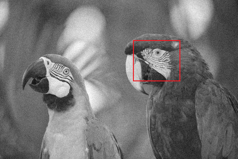
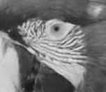
(a)	(b)	(c)

Figure 8: Example of $\mathop{\rm ICTGV}\nolimits^{\mathop{\rm osci}\nolimits}$ denoising. In the top row, the whole image is depicted, while a closeup of the respective marked region is shown in the bottom row. (a) A noisy image. (b) Results of $\mathop{\rm TGV}\nolimits^{2}$-denoising. (c) Results of $\mathop{\rm ICTGV}\nolimits^{\mathop{\rm osci}\nolimits}$ denoising. Parameters were optimised towards best peak signal-to-noise ratio with respect to the ground truth (not shown).

TGV for manifold-valued data.

In different applications in inverse problems and imaging, the data of interest takes values not in a vector space but rather a non-linear space such as a manifold. Examples are sphere-valued data in synthetic aperture radar (SAR) imaging or data with values in the space of positive matrices, equipped with the Fisher–Rao metric, which is used diffusion tensor imaging. Motivated by such applications, TV regularisation has been extended to cope with manifold-valued data, using different approaches and numerical algorithms [67, 128, 190, 97]. A rather simple extension of TV for discrete and finite, univariate signals $(u_{i})_{i}$ living in a complete Riemannian manifold $\mathcal{M}\subset\mathbf{R}^{d}$ with metric $d_{\mathcal{M}}$ is given as

$$\mathop{\rm TV}\nolimits(u)=\sum_{i}d_{\mathcal{M}}(u_{i+1},u_{i}).$$

For this setting, and an extension to bivariate signals, the work [190] provides simple numerical algorithms which yield, in case $\mathcal{M}$ is a Hadamard space, globally optimal solutions of variational TV denoising for manifold-valued data. While this allows in particular to extend edge-preserving regularisation to non-linear geometric data, it can again be observed that TV regularisation has a tendency towards piecewise constant solutions with artificial jump discontinuities. To overcome this, different works have proposed extensions of this approach to higher-order TV [10], the ($\mathop{\rm TV}\nolimits$-$\mathop{\rm TV}\nolimits^{2}$)-infimal convolution [14, 15] and second-order TGV [36, 15]. Here we briefly sketch the main underlying ideas, presented in [36], for an extension of TGV to manifold-valued data. For simplicity, we consider only the case of univariate signals $(u_{i})_{i}$ and assume that length-minimising geodesics are unique (see [36] for the general case and details on the involved differential-geometric concepts).

From the continuous perspective, a natural approach to extend $\mathop{\rm TGV}\nolimits$ for manifold-valued data, at least in a smooth setting, would be to use tangent spaces for first-order derivatives and, for the second-order term, invoke a connection on the manifold for the differentiation of vector fields. In contrast to that, the motivation for the definition of TGV as in [36] was to exploit a discrete setting in order to avoid high-level differential-geometric concepts but rather to come up with a definition of TGV that can be written only in terms of the distance function on the manifold. To this aim, we identify tangential vectors $v\in T_{a}\mathcal{M}$, with $T_{a}\mathcal{M}$ denoting the tangent space at a point $a\in\mathcal{M}$, with point tuples $[a,b]$ via the exponential map $b=\exp_{a}(v)$. A discrete gradient operator then maps a signal $(u_{i})_{i}$ to a sequence of point-tuples $([u_{i},u_{i+1}])_{i}$, where we regard $(\nabla u)_{i}=[u_{i},u_{i+1}]$, which generalises first-order differences in vector spaces, since in this case, $\exp_{u_{i}}(u_{i+1}-u_{i})=u_{i+1}$. Vector fields whose base points are $(u_{i})_{i}$ can then be identified with a sequence $([u_{i},y_{i}])_{i}$ with each $y_{i}\in\mathcal{M}$ and, assuming $D:\mathcal{M}^{2}\times\mathcal{M}^{2}\rightarrow[0,\infty)$ to be an appropriate distance-type function for such tuples, an extension of second-order $\mathop{\rm TGV}\nolimits$ can be given as

$$\mbox{M-}\mathop{\rm TGV}\nolimits((u_{i})_{i})=\min_{(y_{i})_{i}}\ \sum_{i}\alpha_{1}D([u_{i},u_{i+1}],[u_{i},y_{i}])+\alpha_{0}D([u_{i},y_{i}],[u_{i-1},y_{i-1}]).$$

The difficulty here is in particular how to define $D$ for two point tuples with different base points, as those represent vectors in different tangent spaces. To overcome this, a variant for $D$ as proposed in [36] uses the Schild’s ladder [118] construction as a discrete approximation of the parallel transport of vector fields between different tangent spaces. In order to describe this construction, denote by $[u,v]_{t}$ for $u,v\in\mathcal{M}$ and $t\in\mathbf{R}$ the point reached at time $t$ after travelling on the geodesics from $u$ to $v$, i.e., $[u,v]_{t}=\exp_{u}(t\log_{u}(v))$, where $\log$ is the inverse exponential map. Then, the parallel transport of $[u,v]$ (which represents $\log_{u}(v)\in T_{u}\mathcal{M}$) to the base point $x\in\mathcal{M}$ is approximated by $[x,y^{\prime}]$ where $y^{\prime}=[u,[x,v]_{\frac{1}{2}}]_{2}$ (which represents $\log_{x}(y^{\prime})\in T_{x}\mathcal{M}$). Using this, a distance on point tuples, denoted by $D_{S}$, can be given as

$$D_{S}([x,y],[u,v])=d_{\mathcal{M}}(y^{\prime},y)\quad\mbox{ with }\quad y^{\prime}=[u,[x,v]_{\frac{1}{2}}]_{2}.$$

Exploiting the fact that $D_{S}([u,v],[u,w])=d_{\mathcal{M}}(v,w)$ for tuples having the same base point, a concrete realisation of discrete second order $\mathop{\rm TGV}\nolimits$ for manifold-valued data is then given as

$$\mbox{S-}\mathop{\rm TGV}\nolimits((u_{i})_{i})=\min_{(y_{i})_{i}}\ \sum_{i}\alpha_{1}d_{\mathcal{M}}(u_{i+1},y_{i})+\alpha_{0}D_{S}([u_{i},y_{i}],[u_{i-1},y_{i-1}]).$$

The $\mbox{S-}\mathop{\rm TGV}\nolimits$ denoising problem for $(f_{i})_{i}$ some given data with $f_{i}\in\mathcal{M}$ then reads as

$$\min_{(u_{i})_{i}}\ \mbox{S-}\mathop{\rm TGV}\nolimits((u_{i})_{i})+\lambda\sum_{i}d_{\mathcal{M}}(u_{i},f_{i})^{2},$$

and a numerical solution (which can only be guaranteed to deliver stationary points due to non-convexity) can be obtained, for instance, using the cyclic proximal point algorithm [9, 36]. Figure 9 shows the results for this setting using both $\mathop{\rm TV}\nolimits$ and second-order $\mathop{\rm TGV}\nolimits$ regularisation for the denoising of $\mathcal{S}^{2}$ valued image data, which is composed of different blocks of smooth data with sharp interfaces. It can be seen that both TV and TGV are able to recover the sharp interfaces, but TV suffers from piecewise-constancy artefacts which are not present with TGV.

Figure 9: Example of variational denoising for manifold-valued data. The images show noisy $\mathcal{S}^{2}$-valued data (left) which is denoised with TV-regulariser (middle) and TGV-regulariser (right). The sphere $\mathcal{S}^{2}$ is colour-coded with hue and value representing the longitude and latitude, respectively. All parameters are selected optimally.

Image-driven TGV.

In case of denoising problems, i.e., $f\in L^{p}({\Omega})$, second-order $\mathop{\rm TGV}\nolimits$ can be modified to incorporate directional information obtained from $f$, resulting in image-driven TGV (ITGV) [151]. The latter is defined by introducing a diffusion tensor field into the functional:

$$\mathop{\rm ITGV}\nolimits_{\alpha}^{2}(u)=\min_{w\in\mathop{\rm BD}\nolimits(\Omega)}\ \alpha_{1}\int_{\Omega}\ \mathrm{d}{{|{D^{1/2}\nabla u-w}|}}+\alpha_{0}\int_{\Omega}\ \mathrm{d}{{|{\mathcal{E}w}|}}$$

where $D:\overline{\Omega}\to\mathop{\rm Sym}\nolimits^{2}(\mathbf{R}^{d})$ is assumed to be continuous and positive semi-definite in each point. Denoting by $f_{\sigma}=f\ast G_{\sigma}$ a smoothed version of the data $f$ obtained by convolution with a Gaussian kernel $G_{\sigma}$ of variance $\sigma>0$ and suitable extension outside of $\Omega$, the diffusion tensor field $D$ may be chosen according to

$$D=\mathop{\rm id}\nolimits-(1-\mathrm{e}^{-\gamma{|{\nabla f_{\sigma}}|}^{\beta}})\frac{\nabla f_{\sigma}}{{|{\nabla f_{\sigma}}|}}\otimes\frac{\nabla f_{\sigma}}{{|{\nabla f_{\sigma}}|}}$$

with parameters $\gamma>0$ and $\beta>0$. If the smallest eigenvalue of $D$ is uniformly bounded away from $0$ in $\overline{\Omega}$, then $\mathop{\rm ITGV}\nolimits$ admits the same functional-analytic and regularisation properties as second-order TGV. We refer to [151] for an application and numerical results regarding this regularisation approach in stereo estimation.

Non-local TGV.

The concept of non-local total variation (NLTV) [93] can also be transferred to the total generalised variation. Recall that instead of taking the derivative, non-local total variation penalises the differences of the function values of $u$ for each pair of points by virtue of a weight function:

$$\mathop{\rm NLTV}\nolimits(u)=\int_{\Omega}\int_{\Omega}a(x,y){|{u(y)-u(x)}|}\ \mathrm{d}{y}\ \mathrm{d}{x},$$

where the weight function $a:\Omega\times\Omega\to[0,\infty]$ is measurable and a.e. bounded from below by a positive constant. We note that, alternatively, the weight function $a$ may also be chosen as $a(x,y)=|x-y|^{-(\theta+d)}$ with $\theta\in(0,1)$ such that low-order Sobolev–Slobodeckij seminorms can be realised [75]. In the context of non-local total variation, $a$ allows to incorporate a-priori information for the image to reconstruct. For instance, if one already knows disjoint segments $\Omega_{1},\ldots,\Omega_{n}$ where the solution is piecewise constant, one can set

$$a(x,y)=\left\{\begin{array}[]{rl}c_{1}&\mbox{if}\ x,y\in\Omega_{i}\ \mbox{for some}\ i,\\ c_{0}&\mbox{else},\end{array}\right.$$

where $c_{1}\gg c_{0}>0$. This way, the difference between two function values of $u$ in $\Omega_{i}$ is forced to $0$, meaning $u$ is constant in $\Omega_{i}$.

Non-local total generalised variation now gives the possibility to enforce piecewise linearity of $u$ in the segments by incorporating the vector field $w$ corresponding to the slope of the linear part in a non-local cascade. This results in

$$\begin{array}[]{rl}\displaystyle\mathop{\rm NLTGV}\nolimits^{2}(u)=\inf_{w\in L^{1}({\Omega,\mathbf{R}^{d}})}&\displaystyle\int_{\Omega}\int_{\Omega}a_{1}(x,y){|{u(y)-u(x)-w(x)\cdot(y-x)}|}\ \mathrm{d}{y}\ \mathrm{d}{x}\\[6.0pt] &\displaystyle+\int_{\Omega}\int_{\Omega}a_{0}(x,y){|{w(y)-w(x)}|}\ \mathrm{d}{y}\ \mathrm{d}{x}.\end{array}$$

with two weight functions $a_{0},a_{1}:\Omega\times\Omega\to[0,\infty]$, again measurable and bounded a.e. away from zero [153]. In analogy to $\mathop{\rm NLTV}\nolimits$, a-priori information on, for instance, disjoint segments where the sought solution is piecewise linear, allows to choose weight functions such that the associated $\mathop{\rm NLTGV}\nolimits^{2}$ regulariser properly reflect this information. See Figure 10 for a denoising example where non-local TGV turns out to be beneficial, in particular in the regions near the jump discontinuities of sought solution.

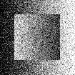
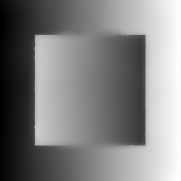
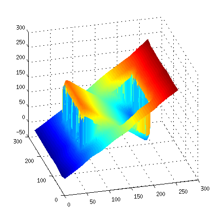
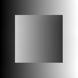
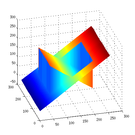
(a)	(b)	(c)

Figure 10: Example for non-local total generalised variation denoising. (a) An noisy piecewise linear image. (b) Results of $\mathop{\rm TGV}\nolimits_{\alpha}^{2}$-denoising together with a surface plot of its graph. (c) Results of non-local TGV-denoising together with a surface plot of its graph. Images taken from [153]. Reprinted by permission from Springer Nature.

6 Numerical algorithms

Tikhonov regularisation with higher-order total variation, its combination via addition or infimal convolution, as well as total generalised variation poses a non-smooth optimisation problem in an appropriate Lebesgue function space. In practice, these minimisation problems are discretized and solved by optimisation algorithms that exploit the structure of the discrete problem. While there are many possibilities for a discretization of the considered regularisation functionals as well as for numerical optimisation, most of the algorithms that can be found in the literature base on finite-difference discretization and first-order proximal optimisation methods. In the following, we provide an overview of the building blocks necessary to solve the considered Tikhonov functional minimisation problems numerically. We will exemplarily discuss the derivation of respective algorithms on the basis of the popular primal-dual algorithm with extragradient [59] and, as alternative, briefly address implicit and preconditioned optimisation methods.

6.1 Discretization of higher-order TV functionals

We discretize the discussed functionals in 2D, higher dimensions follow by analogy. Moreover, for the sake of simplicity, we assume a rectangular domain, i.e., $\Omega={]{0,N_{1}}[}\times{]{0,N_{2}}[}\subset\mathbf{R}^{2}$ for some positive $N_{1},N_{2}\in\mathbf{N}$. A generalisation to non-rectangular domains will be straightforward.

Following essentially the presentation in [37] we first replace $\Omega$ by the discretized grid

$$\Omega_{h}=\{{(i,j)}\ \bigl{|}\ {i,j\in\mathbf{N},\ 1\leq i\leq N_{1},\ 1\leq j\leq N_{2}}\}.$$

One consistent way of discretizing higher-order derivatives is to define partial derivatives as follows: A discrete partial derivative takes the difference between two neighbouring elements in the grid with respect to a specified axis. This difference is associated with the midpoint between the two grid elements, resulting in staggered grids. For a finite sequence of directions $p\in\bigcup_{k\geq 0}\{{1,2}\}^{k}$, this results, on the one hand, in the recursively defined grids

$$\begin{array}[]{rl}\displaystyle\Omega_{h}^{()}&=\Omega_{h},\\ \displaystyle\Omega_{h}^{(1,p_{k},\ldots,p_{1})}&=\{{(i+\frac{1}{2},j)}\ \bigl{|}\ {(i,j),(i+1,j)\in\Omega_{h}^{(p_{k},\ldots,p_{1})}}\}\\ \displaystyle\Omega_{h}^{(2,p_{k},\ldots,p_{1})}&=\{{(i,j+\frac{1}{2})}\ \bigl{|}\ {(i,j),(i,j+1)\in\Omega_{h}^{(p_{k},\ldots,p_{1})}}\}\end{array}$$ (57)

Note that $\Omega_{h}^{p}$ does not depend on the order of the $p_{i}$ and one could use multiindices in $\mathbf{N}^{2}$ instead. Likewise, the discrete partial derivatives recursively given by

$$\begin{array}[]{rl}\partial^{()}u&=u,\\ (\partial^{(1,p_{k},\ldots,p_{1})}_{h}u)_{i,j}&=(\partial^{(p_{k},\ldots,p_{1})}_{h}u)_{i+\frac{1}{2},j}-(\partial^{(p_{k},\ldots,p_{1})}_{h}u)_{i-\frac{1}{2},j},\\ (\partial^{(2,p_{k},\ldots,p_{1})}_{h}u)_{i,j}&=(\partial^{(p_{k},\ldots,p_{1})}_{h}u)_{i,j+\frac{1}{2}}-(\partial^{(p_{k},\ldots,p_{1})}_{h}u)_{i,j-\frac{1}{2}},\end{array}$$ (61)

yield well-defined functions $\partial_{h}^{p}u:\Omega_{h}^{p}\to\mathbf{R}$ for $u:\Omega_{h}\to\mathbf{R}$ which do not depend on the order of the entries in $p$. The discrete gradient $\nabla_{h}^{k}u$ of order $k\geq 1$ for $u:\Omega_{h}\to\mathbf{R}$ is then the tuple that collects all the partial derivatives of order $k$:

$$\nabla_{h}^{k}u=(\partial_{h}^{p}u)_{p\in\{{1,2}\}^{k}}\in\bigtimes_{p\in\{{1,2}\}^{k}}\{u_{p}:\Omega_{h}^{p}\rightarrow\mathbf{R}\}.$$

Note that due to this construction, the partial derivatives $\partial_{h}^{p}u$ are generally defined on different grids. However, in order to define the Frobenius norm of $\nabla^{k}_{h}$, and, consequently, an $\ell^{1}$-type norm, a common grid is needed. There are several possibilities for this task (such as interpolation) which has been studied mainly for the first-order total variation. Here, we discuss a strategy that results in a simple definition of a discrete higher-order total variation. It bases on collecting, for $(i,j)\in\mathbf{Z}^{2}$, all the nearby points in the different $\Omega_{h}^{p}$. This can, for instance, be done by moving half-steps forward and backward in the directions indicated by $p\in\{{1,2}\}^{k}$:

$$(i_{p},j_{p})=(i,j)+\frac{1}{2}\sum_{m=1}^{k}(-1)^{m+1}e_{p_{m}}$$ (62)

where $e_{1},e_{2}$ are the unit vectors in $\mathbf{R}^{2}$. The Frobenius norm in a point $(i,j)\in\mathbf{Z}^{2}$ is then given by

$${|{\nabla_{h}^{k}u}|}_{i,j}=\Bigl{(}\sum_{p\in\{{1,2}\}^{k}}{|{(\partial_{h}^{p}u)_{i_{p},j_{p}}}|}^{2}\Bigr{)}^{1/2},$$ (63)

where $\partial_{h}^{p}u$ is extended by zero outside of $\Omega_{h}^{p}$. Note that here, although $\partial^{p}_{h}$ does not depend on the order of discrete differentiation, the point $(i_{p},j_{p})$ does. Thus, a different Frobenius norm for the $k$-th discrete derivative would be constituted by symmetrisation, which means symmetrising $\nabla_{h}^{k}u$ and taking the Frobenius norm afterwards. In this context, is makes sense to average over the grid points as follows. Denoting by $\alpha(p)\in\mathbf{N}^{2}$ the multiindex associated with $p\in\{{1,2}\}^{k}$, i.e., $\alpha(p)_{i}=\#\{{m}\ \bigl{|}\ {p_{m}=i}\}$, we define

$$(i_{\alpha},j_{\alpha})={{{|{\alpha}|}}\choose{\alpha}}^{-1}\sum_{p\in\{{1,2}\}^{{|{\alpha}|}},\alpha(p)=\alpha}(i_{p},j_{p})$$ (64)

for $(i,j)\in\mathbf{Z}^{2}$ and $\alpha\in\mathbf{N}^{2}$, where ${{{|{\alpha}|}}\choose{\alpha}}=\frac{(\alpha_{1}+\alpha_{2})!}{\alpha_{1}!\alpha_{2}!}$. Then, the grid associated with an $\alpha\in\mathbf{N}^{2}$ reads as

$$\quad\Omega_{h}^{\alpha}=\{{(i_{\alpha},j_{\alpha})}\ \bigl{|}\ {(i,j)\in\mathbf{Z}^{2},\ (i_{p},j_{p})\in\Omega_{h}^{p}\ \mbox{for some}\ p\in\{1,2\}^{k}\ \mbox{with}\ \alpha(p)=\alpha}\},$$

while the $\alpha$-component of the symmetrised gradient is given by

$$(|\!|\!|\partial^{\alpha}_{h}u)_{i_{\alpha},j_{\alpha}}={{{|{\alpha}|}}\choose{\alpha}}^{-1}\sum_{p\in\{{1,2}\}^{{|{\alpha}|}},\alpha(p)=\alpha}(\partial^{p}_{h}u)_{i_{p},j_{p}}$$

where $(i,j)\in\mathbf{Z}^{2}$ is chosen such that $(i_{\alpha},j_{\alpha})\in\Omega_{h}^{\alpha}$ and $(\partial^{p}_{h}u)_{i_{p},j_{p}}$ is zero for points outside of $\Omega_{h}^{p}$. This results in the symmetrised derivative as follows:

$$\mathcal{E}_{h}^{k}u=(|\!|\!|\partial^{\alpha}_{h}u)_{\alpha\in\mathbf{N}^{2},{|{\alpha}|}=k}\in\bigtimes_{\alpha\in\mathbf{N}^{2},{|{\alpha}|}=k}\{{u_{\alpha}:\Omega_{h}^{\alpha}\to\mathbf{R}}\}.$$

The Frobenius norm of $\mathcal{E}_{h}^{k}u$ in a point $(i,j)\in\mathbf{Z}^{2}$ can finally be obtained by

$${|{\mathcal{E}^{k}_{h}u}|}_{i,j}=\Bigl{(}\sum_{\alpha\in\mathbf{N}^{2},{|{\alpha}|}=k}{{{|{\alpha}|}}\choose{\alpha}}{|{(|\!|\!|\partial^{\alpha}_{h}u)_{i_{\alpha},j_{\alpha}}}|}^{2}\Bigr{)}^{1/2}.$$ (65)

Remark 6.1.

For $\alpha\in\mathbf{N}^{2}$ with ${|{\alpha}|}$ even, we have $(i_{\alpha},j_{\alpha})=(i,j)$ for each $(i,j)\in\mathbf{Z}$. Indeed, for $p\in\{{1,2}\}^{{|{\alpha}|}}$ and the reversed tuple $\bar{p}=(p_{{|{\alpha}|}},\ldots,p_{1})$ it holds $\alpha(p)=\alpha(\bar{p})$. Further, either $p=\bar{p}$ leading to $(i_{p},j_{p})=(i,j)$ or $p\neq\bar{p}$ leading to $(i_{p},j_{p})+(i_{\bar{p}},j_{\bar{p}})=2(i,j)$. Consequently, $(i_{\alpha},j_{\alpha})=(i,j)$ according to the definition. In other words, the symmetrisation of the discrete gradient is a natural way of aligning the different grids $\Omega_{h}^{p}$ to a common grid in this case.

For ${|{\alpha}|}$ odd, the grid points still do not align. However, we can say that for $(i,j)$, the point $(i_{\alpha},j_{\alpha})$ lies on the line connecting $(i+\frac{1}{2},j)$ and $(i,j+\frac{1}{2})$. Indeed, for $p\in\{{1,2}\}^{{|{\alpha}|}}$ with $\alpha(p)=\alpha$ we can consider $\bar{p}=(p_{{|{\alpha}|}-1},\ldots,p_{1},p_{{|{\alpha}|}})$. If $p=\bar{p}$, then $(i_{p},j_{p})$ is either $(i+\frac{1}{2},j)$ or $(i,j+\frac{1}{2})$. In the case $p\neq\bar{p}$, the point $\frac{1}{2}(i_{p},j_{p})+\frac{1}{2}(i_{\bar{p}},j_{\bar{p}})$ is either $(i+\frac{1}{2},j)$ or $(i,j+\frac{1}{2})$. As $(i_{\alpha},j_{\alpha})$ is a convex combination of such points, it lies on the line connecting $(i+\frac{1}{2},j)$ and $(i,j+\frac{1}{2})$. Hence, the symmetrisation of the gradient leads to more localised grid points.

We now have everything at hand to define two versions of a discrete total variation of arbitrary order.

Definition 6.2.

Let $k\in\mathbf{N}$, $k\geq 1$ a differentiation order. Then, for $u:\Omega_{h}\to\mathbf{R}$, the discrete total variation is defined as

$$\mathop{\rm TV}\nolimits_{h}^{k}(u)=\|{\nabla_{h}^{k}u}\|_{1}=\sum_{(i,j)\in\mathbf{Z}^{2}}{|{\nabla_{h}^{k}u}|}_{i,j}$$

with ${|{\nabla_{h}^{k}u}|}_{i,j}$ according to (63), and discrete total variation for the symmetrised gradient is defined as

$$\mathop{\rm TV}\nolimits_{h,\mathop{\rm sym}\nolimits}^{k}(u)=\|{\mathcal{E}_{h}^{k}u}\|_{1}=\sum_{(i,j)\in\mathbf{Z}^{2}}{|{\mathcal{E}_{h}^{k}u}|}_{i,j},$$

with ${|{\mathcal{E}_{h}^{k}u}|}_{i,j}$ according to (65).

In order to define a discrete version of the total generalised variation, we still need to discuss the discretization of the total deformation for discrete symmetric tensor fields. For this purpose, we say that the components of a discrete symmetric tensor field of order $l\in\mathbf{N}$, live on the grids $\Omega_{h}^{\alpha}$, resulting in

$$u=(u_{\alpha})_{\alpha\in\mathbf{N}^{2},{|{\alpha}|}=l}\in\bigtimes_{\alpha\in\mathbf{N}^{2},{|{\alpha}|}=l}\{{u_{\alpha}:\Omega_{h}^{\alpha}\to\mathbf{R}}\},$$

realising a discrete symmetric tensor field of order $l$. Its Frobenius norm is given in the points $(i,j)\in\mathbf{Z}^{2}$ according to

$${|{u}|}_{i,j}=\Bigl{(}\sum_{\alpha\in\mathbf{N}^{2},{|{\alpha}|}=l}{{{|{\alpha}|}}\choose{\alpha}}{|{(u_{\alpha})_{i_{\alpha},j_{\alpha}}}|}^{2}\Bigr{)}^{1/2},$$ (66)

which is compatible with (65) if one plugs in $\mathcal{E}_{h}^{l}u$ for some $u:\Omega_{h}\to\mathbf{R}$. The partial derivative of order $k$ described by $p\in\{{1,2}\}^{k}$ applied to $u_{\alpha}$ is then also given by (61), but acts on the grid $\Omega_{h}^{\alpha}$ and results in a discrete function on the grid $\Omega_{h}^{\alpha,p}$ which given in analogy to (57) by replacing $\Omega_{h}$ with $\Omega_{h}^{\alpha}$. The symmetrised derivative $\mathcal{E}_{h}^{k}u$, whose components are indexed by $\beta\in\mathbf{N}^{2}$, ${|{\beta}|}=k+l$, is then defined in a point $(i_{\beta},j_{\beta})\in\Omega_{h}^{\beta}$ where $(i,j)\in\mathbf{Z}^{2}$ by

$$\bigl{(}(\mathcal{E}_{h}^{k}u)_{\beta}\bigr{)}_{i_{\beta},j_{\beta}}={{{|{\beta}|}}\choose{\beta}}^{-1}\sum_{\alpha\in\mathbf{N}^{2},p\in\{{1,2}\}^{k},\alpha+\alpha(p)=\beta}{{{|{\alpha}|}}\choose{\alpha}}(\partial^{p}_{h}u_{\alpha})_{i_{\alpha,p},j_{\alpha,p}}$$ (67)

where

$$(i_{\alpha,p},j_{\alpha,p})=(i_{\alpha},j_{\alpha})+\frac{1}{2}\sum_{m=1}^{k}(-1)^{l+m+1}e_{p_{m}}.$$

This is sufficient to define a discrete total deformation.

Definition 6.3.

Let $k,l\in\mathbf{N}$, $k\geq 1$ and $l\geq 0$. Then, for $u=(u_{\alpha})_{\alpha\in\mathbf{N}^{2},{|{\alpha}|}=l}$, the discrete total deformation of order $k$ is defined as

$$\mathop{\rm TD}\nolimits_{h}^{k}(u)=\|{\mathcal{E}_{h}^{k}u}\|_{1}=\sum_{(i,j)\in\mathbf{Z}^{2}}{|{\mathcal{E}_{h}^{k}u}|}_{i,j},$$

with $\mathcal{E}_{h}^{k}u$ according to (67) and ${|{\,\cdot\,}|}_{i,j}$ according to (66).

For the sake of completeness, the respective definitions for non-symmetric tensor fields of order $l$ read as

$$u=(u_{p})_{p\in\{{1,2}\}^{l}}\in\bigtimes_{p\in\{{1,2}\}^{l}}\{{u_{p}:\Omega_{h}^{p}\to\mathbf{R}}\},\qquad{|{u}|}_{i,j}=\Bigl{(}\sum_{p\in\{{1,2}\}^{l}}{|{(u_{p})_{i_{p},j_{p}}}|}^{2}\Bigr{)}^{1/2},$$ (68)

and the $p$-th component, $p\in\{{1,2}\}^{k+l}$, of the discrete gradient of order $k$ is given as

$$(\nabla_{h}^{k}u)_{p}=\partial_{h}^{(p_{k+l},\ldots,p_{l+1})}u_{(p_{l},\ldots,p_{1})}.$$ (69)

For numerical algorithms, it is necessary to write the discrete total variation and total deformation as the $1$-norm of a (symmetric) tensor with respect to the respective discrete differentiation operator. We therefore introduce the underlying spaces.

Definition 6.4.

Let $l\in\mathbf{N}$, and $q\in[1,\infty]$. The $\ell^{q}$-space of discrete $l$-tensors on $\Omega_{h}$ is given by

$$\ell^{q}(\Omega_{h},\mathcal{T}^{l}(\mathbf{R}^{2}))=\{{u}\ \bigl{|}\ {u=(u_{p})_{p\in\{{1,2}\}^{l}},\ u_{p}:\Omega_{h}^{p}\to\mathbf{R}\ \mbox{for all}\ p\in\{{1,2}\}^{l}}\}$$

with $\Omega_{h}^{p}$ according to (57), and norm

$$\begin{array}[]{rlrrl}\|{u}\|_{q}&=\displaystyle\Bigl{(}\sum_{(i,j)\in\mathbf{Z}^{2}}{|{u}|}_{i,j}^{q}\Bigr{)}^{1/q}&\mbox{if}\ q<\infty,&\quad\|{u}\|_{\infty}&=\displaystyle\max_{(i,j)\in\mathbf{Z}^{2}}{|{u}|}_{i,j},\end{array}$$

with pointwise norm according to (68). The space $\ell^{2}(\Omega_{h},\mathcal{T}^{l}(\mathbf{R}^{2}))$ is equipped with the scalar product

$$\langle{u},\,{v}\rangle_{\ell^{2}(\Omega_{h},{\mathcal{T}^{l}(\mathbf{R}^{2}))}}=\sum_{(i,j)\in\mathbf{Z}^{2}}\sum_{p\in\{{1,2}\}^{l}}(u_{p})_{i_{p},j_{p}}(v_{p})_{i_{p},j_{p}}.$$

Analogously, the $\ell^{q}$-space of discrete symmetric $l$-tensors on $\Omega_{h}$ is defined as

$$\ell^{q}(\Omega_{h},\mathop{\rm Sym}\nolimits^{l}(\mathbf{R}^{2}))=\{{u}\ \bigl{|}\ {u=(u_{\alpha})_{\alpha\in\mathbf{N}^{2},{|{\alpha}|}=l},\ u_{\alpha}:\Omega_{h}^{\alpha}\to\mathbf{R}\ \mbox{for all}\ \alpha\in\mathbf{N}^{2},{|{\alpha}|}=l}\}$$

with an analogous norm using (66) as pointwise norm. The scalar product on $\ell^{2}(\Omega_{h},\mathop{\rm Sym}\nolimits^{l}(\mathbf{R}^{2}))$ is given by

$$\langle{u},\,{v}\rangle_{\ell^{2}(\Omega_{h},{\mathop{\rm Sym}\nolimits^{l}(\mathbf{R}^{2})})}=\sum_{(i,j)\in\mathbf{Z}^{2}}\sum_{\alpha\in\mathbf{N}^{2},{|{\alpha}|}=l}{{{|{\alpha}|}}\choose{\alpha}}(u_{\alpha})_{i_{\alpha},j_{\alpha}}(v_{\alpha})_{i_{\alpha},j_{\alpha}}.$$

For $k\in\mathbf{N}$, Equation (67) then defines a linear operator mapping

$$\mathcal{E}_{h}^{k}:\ell^{2}(\Omega_{h},\mathop{\rm Sym}\nolimits^{l}(\mathbf{R}^{2}))\to\ell^{2}(\Omega_{h},\mathop{\rm Sym}\nolimits^{k+l}(\mathbf{R}^{2}))$$

and (69) induces a linear operator mapping

$$\nabla_{h}^{k}:\ell^{2}(\Omega_{h},\mathcal{T}^{l}(\mathbf{R}^{2}))\to\ell^{2}(\Omega_{h},\mathcal{T}^{k+l}(\mathbf{R}^{2})).$$

The norm of these operators can easily be estimated:

Lemma 6.5.

We have $\|{\nabla_{h}^{k}}\|\leq 8^{k/2}$ and $\|{\mathcal{E}_{h}^{k}}\|\leq 8^{k/2}$ independent of $l$.

Proof.

As $\nabla^{k}_{h}=\nabla_{h}\cdots\nabla_{h}$ on the respective discrete tensor fields, it is sufficient to prove the statement for $k=1$ and $l$ arbitrary. For this purpose, observe that for $u:\Omega_{h}^{p}\to\mathbf{R}$, $p\in\{{1,2}\}^{l}$, we have

$$\|{\partial_{h}^{(1,p_{l},\ldots,p_{1})}u}\|_{2}^{2}=\sum_{(i,j)\in\mathbf{Z}^{2}}{|{\partial_{h}^{(1,p_{l},\ldots,p_{1})}u}|}_{i_{p}+1/2,j_{p}}^{2} \leq 2\sum_{(i,j)\in\mathbf{Z}^{2}}{|{u}|}^{2}_{i+1,j}+{|{u}|}^{2}_{i,j}$$

$$\leq 4\sum_{(i,j)\in\mathbf{Z}^{2}}{|{u}|}_{i,j}^{2}=4\|{u}\|_{2}^{2},$$

and an analogous estimate for $\|{\partial_{h}^{(2,p_{l},\ldots,p_{1})}u}\|_{2}^{2}$. Consequently, $\|{\nabla_{h}u}\|_{2}^{2}\leq 8\|{u}\|_{2}^{2}$ for such $u$. If $u\in\ell^{2}(\Omega_{h},\mathcal{T}^{l}(\mathbf{R}^{2}))$, then

$$\|{\nabla_{h}u}\|_{2}^{2}=\sum_{p\in\{{1,2}\}^{l}}\|{\nabla_{h}u_{p}}\|_{2}^{2}\leq 8\sum_{p\in\{{1,2}\}^{l}}\|{u_{p}}\|_{2}^{2}=8\|{u}\|_{2}^{2},$$

so the claim follows.

For the symmetrised gradient, it is possible to pursue the same strategy since $\mathcal{E}_{h}^{k}=\mathcal{E}_{h}\cdots\mathcal{E}_{h}$ on the respective discrete symmetric tensor fields. Indeed, with the Cauchy–Schwarz inequality and Vandermonde’s identity (which reduces to the standard recurrence relation for binomial coefficients in most cases), one obtains

$${|{\mathcal{E}_{h}u}|}_{i,j}^{2} =\sum_{\beta\in\mathbf{N}^{2},{|{\beta}|}=l+1}{{{|{\beta}|}}\choose{\beta}}\bigl{|}{\bigl{(}(\mathcal{E}_{h}u)_{\beta}\bigr{)}_{i_{\beta},j_{\beta}}}\bigr{|}^{2}$$

$$\leq\sum_{\beta\in\mathbf{N}^{2},{|{\beta}|}=l+1}\ \ \sum_{\alpha\in\mathbf{N}^{2},{|{\alpha}|}=l,p\in\{1,2\},\alpha+\alpha(p)=\beta}{{{|{\alpha}|}}\choose{\alpha}}{|{(\partial^{p}_{h}u_{\alpha})_{i_{\alpha,p},j_{\alpha,p}}}|}^{2}$$

$$=\sum_{p=1}^{2}\sum_{{|{\alpha}|}=l}{{{|{\alpha}|}}\choose{\alpha}}{|{(\partial^{p}_{h}u_{\alpha})_{i_{\alpha,p},j_{\alpha,p}}}|}^{2}=\sum_{p=1}^{2}{|{\partial^{p}_{h}u}|}^{2}_{i_{p},j_{p}}.$$

It is then easy to see that $\|{\mathcal{E}_{h}u}\|_{2}^{2}\leq\sum_{p=1}^{2}\|{\partial_{h}^{p}u}\|_{2}^{2}\leq 8\|{u}\|_{2}^{2}$. ∎

Remark 6.6.

For $p\in\{{1,2}\}^{l}$ and $p_{0}\in\{{1,2}\}$, consider the discrete partial derivative $\partial_{h}^{p_{0}}:\Omega_{h}^{p}\to\Omega_{h}^{(p_{0},p)}$ and its negative adjoint $\partial_{h,0}^{p_{0}}$, i.e., $\langle{\partial_{h}^{p_{0}}u},\,{v}\rangle=-\langle{u},\,{\partial_{h,0}^{p_{0}}v}\rangle$ for $u:\Omega_{h}^{p}\to\mathbf{R}$, $v:\Omega_{h}^{(p_{0},p)}\to\mathbf{R}$. For $u:\Omega_{h}^{(p_{0},p)}\to\mathbf{R}$, this results in

$$(\partial_{h,0}^{p_{0}}u)_{i_{p},j_{p}}=\left\{\begin{array}[]{cc}u_{i_{p}+\frac{1}{2},j_{p}}-u_{i_{p}-\frac{1}{2},j_{p}}&\mbox{if}\ p_{0}=1,\\ u_{i_{p},j_{p}+\frac{1}{2}}-u_{i_{p},j_{p}-\frac{1}{2}}&\mbox{if}\ p_{0}=2,\end{array}\right.$$

for $(i_{p},j_{p})\in\Omega_{h}^{p}$, where $u$ is extended by $0$ outside of $\Omega_{h}^{(p_{0},p)}$. (In contrast, $\partial_{h}^{p_{0}}u$ is only defined for $(i_{p},j_{p})\in\Omega_{h}^{(p_{0},p_{0},p)}$.)

Consequently, the negative adjoint of the discrete gradient induces a divergence for discrete tensor fields $u\in\ell^{2}(\Omega_{h},\mathcal{T}^{l+1}(\mathbf{R}^{2}))$ such that $\mathop{\rm div}\nolimits_{h}u\in\ell^{2}(\Omega_{h},\mathcal{T}^{l}(\mathbf{R}^{2}))$ and

$$(\mathop{\rm div}\nolimits_{h}u)_{p}=\partial^{1}_{h,0}u_{(1,p)}+\partial^{2}_{h,0}u_{(2,p)}$$

for $p\in\{{1,2}\}^{l}$. For the discrete divergence that arises as the negative adjoint of the symmetrised gradient on $\ell^{2}(\Omega_{h},\mathop{\rm Sym}\nolimits^{l}(\mathbf{R}^{d}))$, one has to take the symmetrisation into account: For $u\in\ell^{2}(\Omega_{h},\mathop{\rm Sym}\nolimits^{l+1}(\mathbf{R}^{2}))$, we have

$$(\mathop{\rm div}\nolimits_{h}u)_{\alpha}=\partial_{h,0}^{1}u_{\alpha+e_{1}}+\partial_{h,0}^{2}u_{\alpha+e_{2}}.$$

Here, the operators $\partial_{h,0}^{p_{0}}$ act on functions on the grid $\Omega_{h}^{\alpha+\alpha(p_{0})}$ and yield functions on the grid $\Omega_{h}^{\alpha}$. Note that in the grid point $(i_{\alpha},j_{\alpha})$, these partial derivatives have to be evaluated in the grid points $(i_{\alpha+e_{1}}+\frac{1}{2}(-1)^{l},j_{\alpha+e_{1}})$ and $(i_{\alpha+e_{2}},j_{\alpha+e_{2}}+\frac{1}{2}(-1)^{l})$, respectively. This way, the discrete divergence operator is consistently defined.

6.2 A general saddle-point framework

Having appropriately discretized versions of higher-order regularisation functionals available, we now deal with the numerical solution of corresponding Tikhonov approaches for inverse problems. To this aim, we first consider a general framework and then derive concrete realisations for different regularisation approaches.

Let $\Omega_{h}$ be the discretized grid of Subsection 6.1 and define $U_{h}=\ell^{2}(\Omega_{h})$. We assume a discrete linear forward operator $K_{h}:U_{h}\rightarrow Y_{h}$, with $(Y_{h},\|\cdot\|_{Y_{h}})$ a finite-dimensional Hilbert space, and a proper, convex, lower semi-continuous and coercive discrepancy term $S_{f_{h}}:Y_{h}\rightarrow[0,\infty]$ with corresponding discrete data $f_{h}$ to be given. Further, we define $\mathcal{R}_{\alpha}:U_{h}\rightarrow[0,\infty]$ to be a regularisation functional given in a general form as $\mathcal{R}_{\alpha}(u)=\min_{w\in W_{h}}\|D_{h}(u,w)\|_{1,\alpha}$, with $D_{h}:U_{h}\times W_{h}\rightarrow V_{h}$, $(u,w)\mapsto D_{h}^{1}u+D_{h}^{2}w$ a discrete differential operator and $W_{h},V_{h}$ finite-dimensional Hilbert spaces. The expression $\|\cdot\|_{1,\alpha}$ here denotes an appropriate $\ell^{1}$-type norm weighted using the parameters $\alpha$ and will be specified later for concrete examples. Its dual norm is denoted by $\|{\,\cdot\,}\|_{\infty,\alpha^{-1}}$. We consider the general minimisation problem

$$\min_{u\in U_{h}}\,S_{f_{h}}(K_{h}u)+\mathcal{R}_{\alpha}(u),$$ (70)

for which we will numerically solve the equivalent reformulation

$$\min_{(u,w)\in U_{h}\times W_{h}}\,S_{f_{h}}(K_{h}u)+\|D_{h}(u,w)\|_{1,\alpha}.$$ (71)

Remark 6.7.

Note that here, the auxiliary variable $w$ and the space $W_{h}$ are used to include balancing-type regularisation approaches such as the infimal convolution of two functionals. Setting, for example, $W_{h}=U_{h}$, $V_{h}=\ell^{2}(\Omega,\mathcal{T}^{1}(\mathbf{R}^{2}))\times\ell^{2}(\Omega,\mathcal{T}^{2}(\mathbf{R}^{2}))$, $D_{h}(u,w)=(\nabla_{h}u-\nabla_{h}w,\nabla_{h}^{2}w)$ and $\|(v_{1},v_{2})\|_{1,\alpha}=\alpha_{1}\|v_{1}\|_{1}+\alpha_{2}\|v_{2}\|_{1}$ for positive $\alpha=(\alpha_{1},\alpha_{2})$ yields

$$\mathcal{R}_{\alpha}(u)=\min_{w\in W_{h}}\ \alpha_{1}\|\nabla_{h}u-\nabla_{h}w\|_{1}+\alpha_{2}\|\nabla_{h}^{2}w\|_{1}=\left(\alpha_{1}\mathop{\rm TV}\nolimits\triangle\alpha_{2}\mathop{\rm TV}\nolimits^{2}\right)(u).$$

Total-variation regularisation can, on the other hand, be obtained by choosing $W_{h}=\{0\}$, $V_{h}=\ell^{2}(\Omega_{h},\mathcal{T}^{1}(\mathbf{R}^{2}))$, $D_{h}(u,0)=\nabla_{h}u$ and $\|v\|_{1,\alpha}=\alpha\|v\|_{1}$ for $\alpha>0$.

Remark 6.8.

The dual norm $\|{\,\cdot\,}\|_{\infty,\alpha^{-1}}$ will become relevant in the context of primal-dual algorithms via its Fenchel dual. Indeed, we have the identity $(\|{\,\cdot\,}\|_{X})^{*}=\mathcal{I}_{\{{\|{\,\cdot\,}\|_{X^{*}}\leq 1}\}}$ for $\|{\,\cdot\,}\|_{X}$ the norm of a general Banach space $X$ and $\|{\,\cdot\,}\|_{X^{*}}$ its dual norm on $X^{*}$. This is a consequence of $\langle{w},\,{u}\rangle-\|{w}\|_{X^{*}}\|{u}\|_{X}\leq 0$ for all $u\in X$ and $w\in X^{*}$, so $(\|{\,\cdot\,}\|_{X})^{*}(w)=0$ for $\|{w}\|_{X^{*}}\leq 1$. For $\|{w}\|_{X^{*}}>1$ one can find a $u\in X$, $\|{u}\|_{X}\leq 1$ such that, for a $c>0$, $\langle{w},\,{u}\rangle\geq 1+c\geq\|{u}\|_{X}+c$. For each $t>0$, we get $\langle{w},\,{tu}\rangle-\|{tu}\|_{X}\geq tc$, hence $(\|{\,\cdot\,}\|_{X})^{*}(w)=\infty$.

Remark 6.9.

While the setting of (70) allows to include rather general forward operators $K_{h}$ and discrepancy terms $S_{f_{h}}$, it will still not capture all applications of higher-order regularisation that we consider later in Subsections 7 and 8. It rather comprises a balance between general applicability and uniform presentation, and we will comment on possible extensions later on such that the interested reader should be able to adapt the setting presented here to the concrete problem setting at hand.

From a more general perspective, the reformulation (71) of (70) constitutes a non-smooth, convex optimisation problem of the form

$$\min_{x\in\mathcal{X}}\,\mathcal{F}(\mathcal{K}x)+\mathcal{G}(x),$$ (72)

with $\mathcal{X},\mathcal{Y}$ Hilbert spaces, $\mathcal{F}:\mathcal{Y}\rightarrow[0,\infty]$, $\mathcal{G}:\mathcal{X}\rightarrow[0,\infty]$ proper, convex and lower semi-continuous functionals and $\mathcal{K}:\mathcal{X}\rightarrow\mathcal{Y}$ linear and continuous. For this class of problems, duality-based first-order optimisation algorithms of ascent/descent-type have become very popular in the past years as they are rather generally applicable and yield algorithms for the solution of (72) that provably converge to a global optimum, while allowing a simple implementation and practical stepsize choices, such as constant stepsizes. The algorithm of [56], for instance, constitutes a relatively early step in this direction, as it solves the TV-denoising problem with constant stepsizes in terms of a dual problem.

For problems of the type (72), it is often beneficial to consider a primal-dual saddle-point reformulation instead of the dual problem alone, in particular in view of general applicability. This is given as

$$\min_{x\in\mathop{\rm dom}\nolimits\mathcal{G}}\ \max_{y\in\mathop{\rm dom}\nolimits\mathcal{F}^{*}}\,\langle\mathcal{K}x,y\rangle_{\mathcal{Y}}+\mathcal{G}(x)-\mathcal{F}^{*}(y),$$ (73)

with $\langle\cdot,\cdot\rangle_{\mathcal{Y}}$ denoting the inner product in $\mathcal{Y}$. By interchanging minimum and maximum and minimising with respect to $x$, one further arrives at the dual problem which reads as

$$\max_{y\in\mathcal{Y}}\ -\mathcal{F}^{*}(y)-\mathcal{G}^{*}(-\mathcal{K}^{*}y).$$ (74)

Under certain conditions, the minimum in (72) and maximum in (74) admit the same value and primal/dual solution pairs for (72) an (74) correspond to solutions of the saddle-point problem (73), see below.

Now, indeed, many different algorithmic approaches for solving (73) are nowadays available (see for instance [123, 59, 60, 41, 42]) and which one of them delivers the best performance typically depends on the concrete problem instance. Here, as exemplary algorithmic framework, we consider the popular primal-dual algorithm of [59] (see also [201, 143]), which has the advantage of being simple and yet rather generally applicable.

Conceptually, the algorithm of [59] solves the saddle-point problem (73) via implicit gradient descent and ascent steps with respect to the primal and dual variables, respectively. With $\mathcal{L}(x,y)=\langle\mathcal{K}x,y\rangle_{\mathcal{Y}}+\mathcal{G}(x)-\mathcal{F}^{*}(y)$, carrying out these implicit steps simultaneously in both variables would correspond to computing the iterates $\{{(x^{n},y^{n})}\}$ via

$$\left\{\begin{array}[]{cl}y^{n+1}&=\quad y^{n}+\sigma\partial_{y}\mathcal{L}(x^{n+1},y^{n+1}),\\ x^{n+1}&=\quad x^{n}-\tau\partial_{x}\mathcal{L}(x^{n+1},y^{n+1}),\end{array}\right.$$ (75)

where $\partial_{x}$ and $\partial_{y}$ denotes the subgradient with respect to the first and second variable, respectively, and $\sigma$, $\tau$ are positive constants. To obtain computationally feasible iterations, the implicit step for $y^{n+1}$ in the primal-dual algorithm uses an extrapolation $\overline{x}^{n}=2x^{n}-x^{n-1}$ of the previous iterate instead of $x^{n+1}$, such that the descent and ascent steps decouple and can be re-written as

$$\left\{\begin{array}[]{cl}y^{n+1}&=\quad(\mathop{\rm id}\nolimits+\sigma\partial\mathcal{F}^{*})^{-1}(y^{n}+\sigma\mathcal{K}\overline{x}^{n}),\\ x^{n+1}&=\quad(\mathop{\rm id}\nolimits+\tau\partial\mathcal{G})^{-1}(x^{n}-\tau\mathcal{K}^{*}y^{n+1}),\\ \overline{x}^{n+1}&=\quad 2x^{n+1}-x^{n}.\end{array}\right.$$ (76)

The mappings $(\mathop{\rm id}\nolimits+\sigma\partial\mathcal{F}^{*})^{-1}$ and $(\mathop{\rm id}\nolimits+\tau\partial\mathcal{G})^{-1}$ used here are so-called proximal mappings of $\mathcal{F}^{*}$ and $\mathcal{G}$, respectively, which, as noted in Proposition 6.10 below, are well-defined and single valued whenever $\mathcal{G},\mathcal{F}^{*}$ are proper, convex and lower semi-continuous. The resulting algorithm can then be interpreted as proximal-point algorithm (see [101, 160]) and weak convergence in the sense that $(x^{n},y^{n})\rightharpoonup(x^{*},y^{*})$ for $(x^{*},y^{*})$ being a solution to the saddle-point problem (73) can be ensured for positive stepsize choices $\sigma,\tau$ such that $\sigma\tau\|\mathcal{K}\|^{2}<1$, see for instance [60, 142], or [59] for the finite-dimensional case. In contrast, explicit methods for non-smooth optimisation problems such as subgradient descent, for instance, usually require stepsizes that converge to zero [137] and could stagnate numerically.

Overall, the efficiency of the iteration steps in (76) crucially depends on the ability to evaluate $\mathcal{K}$ and $\mathcal{K}^{*}$ and to compute the proximal mappings efficiently. Regarding the latter, this is possible for a large class of functionals, in particular for many functionals that are defined pointwise, which is one of the reasons for the high popularity of these kind of algorithms. We now consider proximal mappings in more detail and provide concrete examples later on.

Proposition 6.10.

Let $H$ be a Hilbert space, $F:H\to{]{-\infty,\infty}]}$ proper, convex and lower semi-continuous, and $\sigma>0$.

1. Then, the mapping

   $$\mathop{\rm prox}\nolimits_{\sigma F}:H\to H,\qquad u\mapsto\mathop{\rm arg\,min}\limits_{\bar{u}\in H}\ \frac{\|{\bar{u}-u}\|_{H}^{2}}{2}+\sigma F(\bar{u})$$ (77)

   is well-defined.

2. For $u\in H$, $u^{*}=\mathop{\rm prox}\nolimits_{\sigma F}(u)$ solves the inclusion relation

   $$u\in u^{*}+\sigma\partial F(u^{*}),$$

   i.e., $\mathop{\rm prox}\nolimits_{\sigma F}=(\mathop{\rm id}\nolimits+\sigma\partial F)^{-1}$.

3. The mapping $\mathop{\rm prox}\nolimits_{\sigma F}$ is Lipschitz-continuous with constant not exceeding $1$.

Proof.

See, for instance, [177, Proposition IV.1.5, Corollary IV.1.3], or [13, Proposition 12.15, Example 23.3, Corollary 23.10]. ∎

In general, the computation of proximal mappings can be as difficult as solving the original optimisation problem itself. However, if, for instance, the corresponding functional can be “well separated” into simple building blocks, then proximal mappings can be reduced to some basic ones which are simple and easy to compute.

Lemma 6.11.

Let $H=H_{1}\perp\cdots\perp H_{n}$ with closed subspaces $H_{1},\ldots,H_{n}$, the mappings $P_{1},\ldots,P_{n}$ their orthogonal projectors,

$$F(u)=\sum_{i=1}^{n}F_{i}(P_{i}u)$$

with each $F_{i}:H_{i}\to{]{-\infty,\infty}]}$ proper, convex and lower semi-continuous. Then,

$$\mathop{\rm prox}\nolimits_{\sigma F}(u)=\sum_{i=1}^{n}\mathop{\rm prox}\nolimits_{\sigma F_{i}}(P_{i}u).$$

Proof.

This is immediate since the corresponding minimisation problem decouples. ∎

Furthermore, Moreau’s identity (see [159], for instance) provides a relation between the proximal mapping of a function $F$ and the proximal mapping of its dual $F^{*}$ according to

$$u=(\mathop{\rm id}\nolimits+\sigma\partial F)^{-1}(u)+\sigma\Bigl{(}\mathop{\rm id}\nolimits+\frac{1}{\sigma}\partial F^{*}\Bigr{)}^{-1}\Bigl{(}\frac{u}{\sigma}\Bigr{)}.$$ (78)

This immediately implies that for general $\sigma>0$, the computation of $(\mathop{\rm id}\nolimits+\sigma\partial F)^{-1}$ is essentially as difficult as the computation of $(\mathop{\rm id}\nolimits+\sigma\partial F^{*})^{-1}$, in particular the latter can be obtained from the former as follows.

Lemma 6.12.

Let $H$ be a Hilbert space and $F:H\to{]{-\infty,\infty}]}$ be proper, convex and lower semi-continuous. Then, for $\sigma>0$,

$$\mathop{\rm prox}\nolimits_{\sigma F}(u)=u-\sigma\mathop{\rm prox}\nolimits_{\frac{1}{\sigma}F^{*}}\Bigl{(}\frac{u}{\sigma}\Bigr{)},\quad\ \ \mathop{\rm prox}\nolimits_{\sigma F^{*}}(u)=u-\sigma\mathop{\rm prox}\nolimits_{\frac{1}{\sigma}F}\Bigl{(}\frac{u}{\sigma}\Bigr{)}.$$

In some situations, the computation of the proximal mappings of the sum of two functions decouples into the composition of two mappings.

Lemma 6.13.

Let $H$ be a Hilbert space, $F:H\to{]{-\infty,\infty}]}$ be proper, convex and lower semi-continuous and $\sigma>0$.

1. If $F(u)=G(u)+\frac{\alpha}{2}\|u-u_{0}\|_{H}^{2}$ with $G:H\rightarrow{]{-\infty,\infty}]}$ proper, convex and lower semi-continuous, $u_{0}\in H$ and $\alpha>0$, then

   $$\mathop{\rm prox}\nolimits_{\sigma F}(u)=\mathop{\rm prox}\nolimits_{\frac{\sigma}{1+\sigma\alpha}G}\circ\mathop{\rm prox}\nolimits_{\sigma\frac{\alpha}{2}\|\cdot-u_{0}\|_{H}^{2}}(u)=\mathop{\rm prox}\nolimits_{\frac{\sigma}{1+\sigma\alpha}G}\left(\frac{u+\sigma\alpha u_{0}}{1+\sigma\alpha}\right)$$

2. If $H=\mathbf{R}^{M}$ equipped with the Euclidean norm and $F(u)=\sum_{m=1}^{M}\mathcal{I}_{[a_{m},b_{m}]}(u_{m})+F_{m}(u_{m})$ with $\mathop{\rm dom}\nolimits(F_{m})\cap[a_{m},b_{m}]\neq\emptyset$ for each $m=1,\ldots,M$, then

   $$\mathop{\rm prox}\nolimits_{\sigma F}(u)_{m}=\mathop{\rm proj}\nolimits_{[a_{m},b_{m}]}\circ\mathop{\rm prox}\nolimits_{\sigma F_{m}}(u_{m})$$

   for $m=1,\ldots,M$, where

   $$\mathop{\rm proj}\nolimits_{[a_{m},b_{m}]}(t)=\mathop{\rm prox}\nolimits_{\sigma\mathcal{I}_{[a_{m},b_{m}]}}(t)=\left\{\begin{array}[]{cl}t&\mbox{if}\ t\in[a_{m},b_{m}],\\ a_{m}&\mbox{if}\ t<a_{m},\\ b_{m}&\mbox{if}\ t>b_{m},\end{array}\right.$$

   is the projection to $[a_{m},b_{m}]$ in $\mathbf{R}$.

Proof.

Regarding (i), we note that by first-order optimality conditions (additivity of the subdifferential follows from [82, Proposition I.5.6]), we have the following equivalences:

$$u^{*}=\mathop{\rm prox}\nolimits_{\sigma F}(u) \quad\Leftrightarrow\quad 0\in u^{*}-u+\sigma\alpha(u^{*}-u_{0})+\sigma\partial G(u)$$

$$\quad\Leftrightarrow\quad 0\in u^{*}-\frac{u+\sigma\alpha u_{0}}{1+\sigma\alpha}+\frac{\sigma}{1+\sigma\alpha}\partial G(u)$$

$$\quad\Leftrightarrow\quad u^{*}=\mathop{\rm prox}\nolimits_{\frac{\sigma}{1+\sigma\alpha}G}\left(\frac{u+\sigma\alpha u_{0}}{1+\sigma\alpha}\right),$$

which proves the explicit form of $\mathop{\rm prox}\nolimits_{\sigma F}$. The intermediate equality follows from $\mathop{\rm prox}\nolimits_{\sigma\frac{\alpha}{2}\|\cdot-u_{0}\|_{H}^{2}}(u)=\frac{u+\sigma\alpha u_{0}}{1+\sigma\alpha}$, which can again be seen from the optimality conditions.

In order to show (ii), first note that, using Lemma 6.11, it suffices to show the assertion for $F(u)=\mathcal{I}_{[a,b]}(u)+f(u)$ with $u\in\mathbf{R}$, $a\leq b$ and $f:\mathbf{R}\to{]{-\infty,\infty}]}$ proper, convex and lower semi-continuous such that $\mathop{\rm dom}\nolimits(f)\cap[a,b]\neq\emptyset$. Also, the identity $\mathop{\rm prox}\nolimits_{\sigma\mathcal{I}_{[a,b]}}=\mathop{\rm proj}\nolimits_{[a,b]}$ as well as the explicit form of the projection is immediate. Now, denote by $u^{*}=\mathop{\rm proj}\nolimits_{[a,b]}\circ\mathop{\rm prox}\nolimits_{\sigma f}(u)$ and write it as $u^{*}=\nu u_{F}+(1-\nu)u_{f}$ with $u_{F}=\mathop{\rm prox}\nolimits_{\sigma F}(u)$ and $u_{f}=\mathop{\rm prox}\nolimits_{\sigma f}(u)$ and $\nu\in[0,1]$. To see that this is possible, note that in case of $u_{f}\in[a,b]$, $u^{*}=u_{f}$, in case $u_{f}<a$ we have that $u_{f}<a=u^{*}\leq u_{F}$ and similarly in case of $u_{f}>b$. But, with $E(\bar{u})=\frac{|\bar{u}-u|^{2}}{2}+\sigma f(\bar{u})$, convexity and minimality of $u_{f}$ implies that

$$E(u^{*})\leq\nu E(u_{F})+(1-\nu)E(u_{f})\leq\nu E(u_{F})+(1-\nu)E(u_{F})=E(u_{F}).$$

Since both $u^{*}$ and $u_{F}$ are in $[a,b]$, the result follows from uniqueness of minimizers. ∎

In the following we provide some examples of explicit proximal mappings for some particular choices of $F$ that are relevant for applications. For additional examples and further, general results on proximal mappings, we refer to [13, 65].

Lemma 6.14.

Let $H$ be a Hilbert space, $\sigma>0$ and $F:H\rightarrow{]{-\infty,\infty}]}$. Then, the following identities hold.

1. For $F(u)=\frac{\alpha}{2}\|{u-f}\|_{H}^{2}$ with $f\in H$, $\alpha>0$,

   $$\mathop{\rm prox}\nolimits_{\sigma F}(u)=\frac{u+\alpha\sigma f}{1+\alpha\sigma},\qquad\mathop{\rm prox}\nolimits_{\sigma F^{*}}(u)=\frac{u-\sigma f}{1+\sigma/\alpha}.$$

2. For $F=\mathcal{I}_{C}$ for some non-empty, convex and closed set $C\subset H$,

   $$\mathop{\rm prox}\nolimits_{\sigma F}=\mathop{\rm proj}\nolimits_{C},$$

   with $\mathop{\rm proj}\nolimits_{C}$ denoting the orthogonal projection onto $C$.

3. For $F(u)=G(u-u_{0})$ with $G:H\rightarrow{]{-\infty,\infty}]}$ and $u_{0}\in H$,

   $$\mathop{\rm prox}\nolimits_{\sigma F}(u)=\mathop{\rm prox}\nolimits_{\sigma G}(u-u_{0})+u_{0}.$$

4. For $H=\mathcal{H}_{1}\times\cdots\times\mathcal{H}_{M}$ product of the Hilbert spaces $\mathcal{H}_{1},\ldots,\mathcal{H}_{M}$, $\|{u}\|_{H}^{2}=\sum_{m=1}^{M}|u_{m}|_{\mathcal{H}_{m}}^{2}$ with each ${|{\,\cdot\,}|_{\mathcal{H}_{m}}}$ denoting the norm on $\mathcal{H}_{m}$, $\alpha\in{]{0,\infty}[}^{M}$, and $F=\mathcal{I}_{\{\|\cdot\|_{\infty,\alpha^{-1}}\leq 1\}}$ where $\|u\|_{\infty,\alpha^{-1}}=\max_{m=1,\ldots,M}\alpha_{m}^{-1}|u_{m}|_{\mathcal{H}}$,

   $$\mathop{\rm prox}\nolimits_{\sigma F}(u)_{m}=\mathop{\rm proj}\nolimits_{\{|\,\cdot\,|_{\mathcal{H}_{m}}\leq\alpha_{m}\}}(u_{m})=\frac{u_{m}}{\max\{1,\alpha_{m}^{-1}{|{u_{m}}|}_{\mathcal{H}_{m}}\}}.$$

5. In the situation of (iv) and $F(u)=\sum_{m=1}^{M}\alpha_{m}|u_{m}|_{\mathcal{H}_{m}}$,

   $$\mathop{\rm prox}\nolimits_{\sigma F}(u)_{m}=\left\{\begin{array}[]{cl}(1-\sigma\alpha_{m}|u_{m}|_{\mathcal{H}_{m}}^{-1})u_{m}&\mbox{if }|u_{m}|_{\mathcal{H}_{m}}>\sigma\alpha_{m},\\ 0&\mbox{else, }\end{array}\right.$$

   and

   $$\mathop{\rm prox}\nolimits_{\sigma F^{*}}(u)_{m}=\mathop{\rm proj}\nolimits_{\{|\,\cdot\,|_{\mathcal{H}_{m}}\leq\alpha_{m}\}}(u_{m})$$

   with $\mathop{\rm proj}\nolimits_{\{|\,\cdot\,|_{\mathcal{H}_{m}}\leq\alpha_{m}\}}$ as in (iv).

Proof.

The assertion on $\mathop{\rm prox}\nolimits_{\sigma F}$ in (i) follows from first-order optimality conditions as in Lemma 6.13, the assertion on $\mathop{\rm prox}\nolimits_{\sigma F^{*}}$ is a consequence of Lemma 6.12. Assertion (ii) is immediate from the definition of the orthogonal projection in Hilbert spaces and (iii) follows from a simple change of variables for the minimisation problem in the definition of the proximal mapping. Regarding (iv), using Lemma 6.11 and noting that $\|{u}\|_{\infty,\alpha^{-1}}\leq 1$ if and only if ${|{u_{m}}|_{\mathcal{H}_{m}}}\leq\alpha_{m}$ for $m=1,\ldots,M$, it suffices to show that for each $u_{m}\in\mathcal{H}_{m}$ and $m=1,\ldots,M$,

$$\mathop{\rm proj}\nolimits_{\{|\cdot|_{\mathcal{H}_{m}}\leq\alpha_{m}\}}(u_{m})=\frac{u_{m}}{\max\{1,\alpha_{m}^{-1}{|{u_{m}}|}_{\mathcal{H}_{m}}\}}.$$

To this aim, observe that by definition of the projection in Hilbert spaces,

$$\mathop{\rm proj}\nolimits_{\{|\cdot|_{\mathcal{H}_{m}}\leq\alpha_{m}\}}(u_{m}) =\mathop{\rm arg\,min}\limits_{|\bar{u}|_{\mathcal{H}_{m}}\leq\alpha_{m}}|\bar{u}-u_{m}|_{\mathcal{H}_{m}}=\mathop{\rm arg\,min}\limits_{|\bar{u}|^{2}_{\mathcal{H}_{m}}\leq\alpha_{m}^{2}}|\bar{u}-u_{m}|^{2}_{\mathcal{H}_{m}}$$

$$=\mathop{\rm arg\,min}\limits_{\bar{u}_{1}\in\mathop{\rm span}\nolimits\{u_{m}\},\ \bar{u}_{2}\in\mathop{\rm span}\nolimits\{u_{m}\}^{\perp},\atop|\bar{u}_{1}|^{2}_{\mathcal{H}_{m}}+|\bar{u}_{2}|^{2}_{\mathcal{H}_{m}}\leq\alpha_{m}^{2}}|\bar{u}_{1}-u_{m}|^{2}_{\mathcal{H}_{m}}+|\bar{u}_{2}|^{2}_{\mathcal{H}_{m}}$$

$$=u_{m}\Biggl{(}\mathop{\rm arg\,min}\limits_{t\in\mathbf{R},\ |tu_{m}|^{2}_{\mathcal{H}}\leq\alpha_{m}^{2}}|t-1|^{2}|u_{m}|^{2}_{\mathcal{H}_{m}}\Biggr{)}.$$

From this, it is easy to see that the minimum in the last line is achieved for $t=1$ in case $|u_{m}|_{\mathcal{H}_{m}}\leq\alpha_{m}$ and $t=\alpha_{m}/|u_{m}|_{\mathcal{H}_{m}}$ otherwise, from which the explicit form of the projection follows. Considering assertion (v), we have by Remark 6.8 that

$$F^{*}(u)=\sum_{m=1}^{M}(\alpha_{m}{|{\,\cdot\,}|_{\mathcal{H}_{m}}})^{*}(u_{m})=\sum_{m=1}^{M}\mathcal{I}_{\{{{|{\,\cdot\,}|_{\mathcal{H}_{m}}}\leq\alpha_{m}}\}}(u_{m})=\mathcal{I}_{\{{\|{\,\cdot\,}\|_{\infty,\alpha^{-1}}\leq 1}\}}(u),$$

so the statements follow by Lemma 6.12 and assertion (iv). ∎

Now considering the minimisation problem (71), our approach is to rewrite it as a saddle-point problem such that, when applying the iteration (76), the involved proximal mappings decouple into simple and explicit mappings. To achieve this while allowing for general forward operators $K_{h}$, we dualise both the regularisation and the data-fidelity term and arrive at the following a saddle-point reformulation of (71):

$$\min_{(u,w)\in U_{h}\times W_{h}}\ \max_{(v,\lambda)\in V_{h}\times Y_{h}}\,\langle D_{h}(u,w),v\rangle_{V_{h}}+\langle K_{h}u,\lambda\rangle_{Y_{h}}-\mathcal{I}_{\{{\|{\,\cdot\,}\|_{\infty,\alpha^{-1}}\leq 1}\}}(v)-S_{f_{h}}^{*}(\lambda),$$ (79)

recalling that the dual norm of $\|{\,\cdot\,}\|_{1,\alpha}$ is denoted by $\|{\,\cdot\,}\|_{\infty,\alpha^{-1}}$ and that $(\|\,\cdot\,\|_{1,\alpha})^{*}=\mathcal{I}_{\{\|\,\cdot\,\|_{\infty,\alpha^{-1}}\leq 1\}}$, see Remark 6.8. The following lemma provides some instances of $\|{\,\cdot\,}\|_{1,\alpha}$ that arise in the context of higher-order TV regularisers and its generalisations. In particular, for these instances, the corresponding dual norm $\|{\,\cdot\,}\|_{\infty,\alpha^{-1}}$ and the proximal mappings $\mathop{\rm prox}\nolimits_{\sigma\mathcal{I}_{\{{\|{\,\cdot\,}\|_{\infty,\alpha^{-1}}\leq 1}\}}}=\mathop{\rm proj}\nolimits_{\{{\|{\,\cdot\,}\|_{\infty,\alpha^{-1}}\leq 1}\}}$ will be provided. Concrete examples will be discussed in Example 6.18 below.

Lemma 6.15.

With $M\in\mathbf{N}$, $\alpha\in{]{0,\infty}[}^{M}$, $l_{1},\ldots,l_{M}\in\mathbf{N}$, and $\mathcal{H}_{m}\in\{\mathcal{T}^{l_{m}}(\mathbf{R}^{2}),\mathop{\rm Sym}\nolimits^{l_{m}}(\mathbf{R}^{2})\}$ for $m=1,\ldots,M$, let

$$V_{h}=\bigtimes_{m=1}^{M}\ell^{2}(\Omega_{h},\mathcal{H}_{m})\quad\mbox{and}\quad\|v\|_{1,\alpha}=\sum_{m=1}^{M}\alpha_{m}\|v_{m}\|_{1},$$

for $v=(v_{1},\ldots,v_{M})\in V_{h}$, where $V_{h}$ is equipped with the induced inner product $\langle u,v\rangle_{V_{h}}=\sum_{m=1}^{M}\langle u_{m},v_{m}\rangle_{\ell^{2}(\Omega_{h},\mathcal{H}_{m})}$ and norm, and the $1$-norm on each $\ell^{2}(\Omega,\mathcal{H}_{M})$ is given in Definition 6.4. Then, the dual norm $\|{\,\cdot\,}\|_{\infty,\alpha^{-1}}$ satisfies

$$\|v\|_{\infty,\alpha^{-1}}=\max_{m=1,\ldots,M}\ \alpha_{m}^{-1}\|v_{m}\|_{\infty},$$

with the $\infty$-norm again according to Definition 6.4. Further, we have, for $m=1,\ldots,M$, that

$$\mathop{\rm prox}\nolimits_{\sigma(\|\,\cdot\,\|_{1,\alpha})^{*}}(v)_{m} =\mathop{\rm proj}\nolimits_{\{\|\cdot\|_{\infty,\alpha^{-1}}\leq 1\}}(v)_{m}=\frac{v_{m}}{\max\{1,\alpha_{m}^{-1}|v_{m}|_{\mathcal{H}_{m}}\}},$$

where the right-hand side has to be interpreted in the pointwise sense, i.e., for $u\in\ell^{2}(\Omega_{h},\mathcal{H}_{m})$ and $(i,j)\in\Omega_{h}$, it holds that $\bigl{(}\max\{1,\alpha_{m}^{-1}{|{u}|_{\mathcal{H}_{m}}}\}^{-1}u\bigr{)}_{i,j}=\max\{1,\alpha_{m}^{-1}{|{u_{i,j}}|_{\mathcal{H}_{m}}}\}^{-1}u_{i,j}$.

Proof.

By definition, we have for $u,v\in V_{h}$ with $\|{u}\|_{1,\alpha}\leq 1$ that

$$\langle{v},\,{u}\rangle_{V_{h}}\leq\sum_{m=1}^{M}\alpha_{m}^{-1}\|{v_{m}}\|_{\infty}\alpha_{m}\|{u_{m}}\|_{1}\leq\max_{m=1,\ldots,M}\alpha_{m}^{-1}\|{v_{m}}\|_{\infty}=\max_{m=1,\ldots,M,\atop(i,j)\in\Omega_{h}}\alpha_{m}^{-1}{|{(v_{m})_{i,j}}|_{\mathcal{H}_{m}}},$$

hence, $\|{v}\|_{\infty,\alpha^{-1}}\leq\max_{m=1,\ldots,M}\alpha_{m}^{-1}\|{v_{m}}\|_{\infty}$. With $(m,i,j)$ a maximising argument of the right-hand side above, equality follows, in case of $v\neq 0$, from choosing $u$ according to $(u_{m})_{i,j}=\alpha_{m}^{-1}(v_{m})_{i,j}/{|{(v_{m})_{i,j}}|_{\mathcal{H}_{m}}}$ and $0$ everywhere else. The case $v=0$ is trivial. Also, since $\Omega_{h}=\{{1,\ldots,N_{1}}\}\times\{{1,\ldots,N_{2}}\}$ is finite, one can interpret each $\ell^{2}(\Omega,\mathcal{H}_{m})$ as $\mathcal{H}_{m}^{N_{1}N_{2}}$, such that Lemma 6.14 (v) applied to $H=V_{h}=\mathcal{H}_{1}^{N_{1}N_{2}}\times\cdots\times\mathcal{H}_{M}^{N_{1}N_{2}}$ immediately yields the stated pointwise identity for the proximal mapping/projection. ∎

Under mild assumptions on $S_{f_{h}}$, equivalence of the primal problem (71) and the saddle-point problem (79) indeed holds and existence of a solution to both (as well as a corresponding dual problem) can be ensured.

Proposition 6.16.

Under the assumptions stated for problem (71), there exists a solution. Further, if $S_{f_{h}}$ is such that $Y_{h}=\bigcup_{t\geq 0}t\bigl{(}\mathop{\rm dom}\nolimits(S_{f_{h}})+\mathop{\rm rg}\nolimits({K_{h}})\bigr{)}$, then there exists a solution to the dual problem

$$\max_{(v,\lambda)\in V_{h}\times Y_{h}}-\mathcal{I}_{\{0\}}\bigl{(}(D_{h}^{1})^{*}v+K_{h}^{*}\lambda\bigr{)}-\mathcal{I}_{\{0\}}\bigl{(}(D_{h}^{2})^{*}v\bigr{)}-\mathcal{I}_{\{{\|{\,\cdot\,}\|_{\infty,\alpha^{-1}}\leq 1}\}}(v)-S_{f_{h}}^{*}(\lambda)$$ (80)

and to the saddle-point problem (79). Further, strong duality holds and the problems are equivalent in the sense that $((u,w),(v,\lambda))$ is a solution to (79) if and only if $(u,w)$ solves (71) and $(v,\lambda)$ solves (80).

Proof.

At first note that existence for (71) can be shown as in Theorem 3.26. By virtue of Theorem 5.7, choosing $X=U_{h}\times W_{h}$, $Y=V_{h}\times Y_{h}$, $F:X\to{]{-\infty,\infty}]}$ as $F=0$, $G:Y\to{]{-\infty,\infty}]}$ as $G(v,\lambda)=\|{v}\|_{1,\alpha}+S_{f_{h}}(\lambda)$, and $\Lambda:X\to Y$ as $\Lambda(u,w)=\bigl{(}D_{h}(u,w),K_{h}u\bigr{)}$, we only need to verify (39) to obtain existence of dual solutions and strong duality. But since $\mathop{\rm dom}\nolimits(F)=X$ and $\mathop{\rm dom}\nolimits(G)=V_{h}\times\mathop{\rm dom}\nolimits(S_{f_{h}})$, the latter condition is equivalent to $Y_{h}=\bigcup_{t\geq 0}t\bigl{(}\mathop{\rm dom}\nolimits(S_{f_{h}})+\mathop{\rm rg}\nolimits({K_{h}})\bigr{)}$. Also, since $F^{*}=\mathcal{I}_{\{{0}\}}$ and $(\|{\,\cdot\,}\|_{1,\alpha})^{*}=\mathcal{I}_{\{{\|{\,\cdot\,}\|_{\infty,\alpha^{-1}}\leq 1}\}}$, see Remark 6.8, the maximisation problem in (40) corresponds to (80). Finally, the equivalence of the saddle-point problem (79) to (71) and (80) then follows from [82, Proposition III.3.1]. ∎

Remark 6.17.

In some applications, it is beneficial to add an additional penalty term on $u$ in form of $\Phi:U_{h}\to[0,\infty]$ proper, convex and lower semi-continuous to the energy of (71), whereas in other situations when $u\mapsto S_{f_{h}}(K_{h}u)$ has a suitable structure, a dualization of the data term is not necessary, see the discussion below. Regarding the former, the differences when extending Proposition 6.16 is that existence for the primal problem needs to be shown differently and that the domain of $\Phi$ needs to be taken into account for obtaining strong duality. Existence can, for instance, be proved when assuming that either $\Phi$ is the indicator function of a polyhedral set (see [35, Proposition 1]), or that $\ker(K_{h})\cap\ker(D_{h})=\{0\}$. Duality is further obtained when $Y_{h}=\bigcup_{t\geq 0}t\bigl{(}\mathop{\rm dom}\nolimits(S_{f_{h}})-K_{h}\mathop{\rm dom}\nolimits(\Phi)\bigr{)}$. Regarding the latter, a version of Proposition 6.16 without the dualization of the data term $S_{f_{h}}(K_{h}u)$ holds even without the assumption on the domain of $S_{f_{h}}$, however, with a different associated dual problem and saddle-point problem.

In particular, not dualising the data term has impact on the primal-dual optimisation algorithms. In view of the iteration (76), the evaluation of the proximal mapping for $u\mapsto S_{f_{h}}(K_{h}u)$ then becomes necessary, so this dualization strategy is only practical if the latter proximal mapping can easily be computed. Furthermore, in case of a sufficiently smooth data term, dualization of $S_{f_{h}}$ can also be avoided by using explicit descent steps for $S_{f_{h}}$ instead of proximal mappings, where the Lipschitz constant of the derivative of $S_{f_{h}}$ usually enters in the stepsize bound. See [60] for an extension of the primal-dual algorithm in that direction.

In view of Proposition 6.16, we now address the numerical solution of the saddle-point problem (79). Applying the iteration (76), this results in Algorithm 1, which is given in a general form. A concrete implementation still requires an explicit form of the proximal mapping $\mathop{\rm prox}\nolimits_{\sigma S_{f_{h}}^{*}}$, a concrete choice of $V_{h}$, $W_{h}$ and $D_{h}$ as well as an estimate on $\|(D_{h},K_{h})\|$ for the stepsize choice and a suitable stopping criterion. These building blocks will now be provided for different choices of $\mathcal{R}_{\alpha}$ and $S_{f_{\alpha}}$ in a way that they can be combined to a arrive at a concrete, application-specific algorithm. After that, two examples will be discussed.

1:function Tikhonov($K_{h}$, $f_{h}$, $\alpha$)

2:     $(u,w,\overline{u},\overline{w})\leftarrow(0,0,0,0),(v,\lambda)\leftarrow(0,0)$

3:     choose $\sigma,\tau>0$ such that $\sigma\tau\left\|\left(\begin{array}[]{cc}D_{h}^{1}&D_{h}^{2}\\ K_{h}&0\end{array}\right)\right\|^{2}<1$

4:     repeat

5:         Dual updates

6:         $v\leftarrow\mathop{\rm proj}\nolimits_{\{\|\cdot\|_{\infty,\alpha^{-1}}\leq 1\}}\left(v+\sigma(D_{h}^{1}\overline{u}+D_{h}^{2}\overline{w})\right)$

7:         $\lambda\leftarrow\mathop{\rm prox}\nolimits_{\sigma S_{f_{h}}^{*}}(\lambda+\sigma K_{h}\overline{u})$

8:         Primal updates

9:         $u_{+}\leftarrow u-\tau\bigl{(}(D_{h}^{1})^{*}v+K_{h}^{*}\lambda\bigr{)}$

10:         $w_{+}\leftarrow w-\tau\bigl{(}(D_{h}^{2})^{*}v\bigr{)}$

11:         Extrapolation and update

12:         $(\overline{u},\overline{w})\leftarrow 2(u_{+},w_{+})-(u,w)$

13:         $(u,w)\leftarrow(u_{+},w_{+})$

14:     until stopping criterion fulfilled

15:     return $u$

16:end function

Algorithm 1 Primal-dual scheme for the numerical solution of (79)

Proximal mapping of $S_{f_{h}}^{*}$.

Depending on the application of interest, and in particular on the assumption on the underlying measurement noise, different choices of $S_{f_{h}}$ are reasonable. The one which is probably most relevant in practice is

$$S_{f_{h}}(\lambda)=\frac{1}{2}\|\lambda-f_{h}\|_{2}^{2},$$

which, from a statistical perspective, is the right choice under the assumption of Gaussian noise. In this case, as discussed in Lemma 6.14, the proximal mapping of the dual is given as

$$\mathop{\rm prox}\nolimits_{\sigma S_{f_{h}}^{*}}(\lambda)=\frac{\lambda-\sigma f_{h}}{1+\sigma}.$$

A second, practically relevant choice is the Kullback-Leibler divergence as in (2). For discrete data $\bigl{(}(f_{h})_{i}\bigr{)}_{i}$ satisfying $(f_{h})_{i}\geq 0$ for each $i$, and a corresponding discrete signal $(\lambda_{i})_{i}$, this corresponds to

$$S_{f_{h}}(\lambda)=\mathop{\rm KL}\nolimits(\lambda,f_{h})=\left\{\begin{array}[]{ll}\sum_{i}\lambda_{i}-(f_{h})_{i}-(f_{h})_{i}\log(\frac{\lambda_{i}}{(f_{h})_{i}})&\mbox{if }\lambda_{i}\in{[{0,\infty}[}\mbox{ for all }i,\\ \infty&\mbox{else,}\end{array}\right.$$ (81)

where we again use the convention $(f_{h})_{i}\log(0)=-\infty$ for $(f_{h})_{i}>0$ and $0\log(\frac{\lambda_{i}}{0})=0$ whenever $\lambda_{i}\geq 0$. A direct computation (see for instance [121]) shows that in this case

$$\mathop{\rm prox}\nolimits_{\sigma S_{f_{h}}^{*}}(\lambda)_{i}=\lambda_{i}-\frac{\lambda_{i}-1+\sqrt{(\lambda_{i}-1)^{2}+4\sigma(f_{h})_{i}}}{2}.$$

Another choice that is relevant in the presence of strong data outliers (e.g., due to transmission errors) is

$$S_{f_{h}}(\lambda)=\|\lambda-f_{h}\|_{1}$$

in which case

$$\mathop{\rm prox}\nolimits_{\sigma S_{f_{h}}^{*}}(\lambda)_{i}=\frac{\lambda_{i}-\sigma(f_{h})_{i}}{\max\{1,|\lambda_{i}-\sigma(f_{h})_{i}|\}}$$

can be obtained from Lemmas 6.12 and 6.14.

As already mentioned in Remark 6.17, in case the discrepancies term is not dualised, a corresponding version of the algorithm of [59] requires the proximal mappings of $\tau S_{f_{h}}$ which can either be computed directly or obtained from $\mathop{\rm prox}\nolimits_{\sigma S_{f_{h}}^{*}}$ using Moreau’s identity as in Lemma 6.12. Further, there are many other choices of $S_{f_{h}}$ for which the $\mathop{\rm prox}\nolimits_{\sigma S_{f_{h}}^{*}}$ is simple and explicit, such as, for instance, equality constraints on a subdomain in the case of image inpainting or box constraints in case of dequantization or image decompression.

Choice of $\mathcal{R}_{\alpha}$ and proximal mapping.

As we show now, the general form $\mathcal{R}_{\alpha}(u)=\min_{w\in W_{h}}\|D_{h}(u,w)\|_{1,\alpha}$ covers all higher-order regularisation approaches discussed in the previous sections.

Example 6.18.

Higher-order total variation.

The choice $\mathcal{R}_{\alpha}(u)=\alpha\|\nabla^{k}u\|_{1}$, with $k\geq 1$ the order of differentiation, can be realised with

$$W_{h}=\{0\},\quad V_{h}=\ell^{2}(\Omega_{h},\mathcal{T}^{k}(\mathbf{R}^{2})),\quad D_{h}=\nabla_{h}^{k},\quad\|v\|_{1,\alpha}=\alpha\|v\|_{1},$$

which yields, according to Lemma 6.15, for $(i,j)\in\Omega_{h}$ that

$$\mathop{\rm proj}\nolimits_{\{\|\cdot\|_{\infty,\alpha^{-1}}\leq 1\}}(v)_{i,j}=\mathop{\rm proj}\nolimits_{\{\|\cdot\|_{\infty}\leq\alpha\}}(v)_{i,j}=\frac{v_{i,j}}{\max\{1,\alpha^{-1}|v|_{i,j}\}}.$$ (82)

Here, we used that whenever $W_{h}=\{0\}$, one can ignore the second argument of $D_{h}:U_{h}\times W_{h}\to V_{h}$ and regard it as operator $D_{h}:U_{h}\rightarrow V_{h}$.

Sum of higher-order TV functionals.

The choice $\mathcal{R}_{\alpha}(u)=\alpha_{1}\|\nabla_{h}^{k_{1}}u\|_{1}+\alpha_{2}\|\nabla_{h}^{k_{2}}u\|_{1}$, with $k_{2}>k_{1}\geq 1$ and $\alpha_{i}>0$ for $i=1,2$ differentiation orders and weighting parameters, respectively, can be realised with

$$\begin{array}[]{l}W_{h}=\{0\},\quad V_{h}=\ell^{2}(\Omega_{h},\mathcal{T}^{k_{1}}(\mathbf{R}^{2}))\times\ell^{2}(\Omega_{h},\mathcal{T}^{k_{2}}(\mathbf{R}^{2}))\quad D_{h}=\left(\begin{array}[]{c}\nabla_{h}^{k_{1}}\\ \nabla_{h}^{k_{2}}\end{array}\right),\\ \|(v_{1},v_{2})\|_{1,\alpha}=\alpha_{1}\|v_{1}\|_{1}+\alpha_{2}\|v_{2}\|_{1},\end{array}$$

and yields, according to Lemma 6.15,

$$\mathop{\rm proj}\nolimits_{\{\|\cdot\|_{\infty,\alpha^{-1}}\leq 1\}}(v_{1},v_{2})=\left(\mathop{\rm proj}\nolimits_{\{\|\cdot\|_{\infty}\leq\alpha_{1}\}}(v_{1}),\ \mathop{\rm proj}\nolimits_{\{\|\cdot\|_{\infty}\leq\alpha_{2}\}}(v_{2})\right)$$ (83)

with $\mathop{\rm proj}\nolimits_{\{\|\cdot\|_{\infty}\leq\alpha_{i}\}}$ as in (82).

Infimal convolution of higher-order TV functionals.

The infimal convolution

$$\mathcal{R}_{\alpha}(u)=\min_{w\in\ell^{2}(\Omega_{h})}\alpha_{1}\|\nabla_{h}^{k_{1}}u-\nabla_{h}^{k_{1}}w\|_{1}+\alpha_{2}\|\nabla_{h}^{k_{2}}w\|_{1}$$

can be realised via

$$\begin{array}[]{l}W_{h}=\ell^{2}(\Omega_{h}),\quad V_{h}=\ell^{2}(\Omega_{h},\mathcal{T}^{k_{1}}(\mathbf{R}^{2}))\times\ell^{2}(\Omega_{h},\mathcal{T}^{k_{2}}(\mathbf{R}^{2})),\\[3.0pt] D_{h}=(D_{h}^{1}\,|\,D_{h}^{2})=\left(\begin{array}[]{c}\nabla_{h}^{k_{1}}\\ 0\end{array}\left|\begin{array}[]{c}-\nabla_{h}^{k_{1}}\\ \nabla_{h}^{k_{2}}\end{array}\right)\right.,\quad\|(v_{1},v_{2})\|_{1,\alpha}=\alpha_{1}\|v_{1}\|_{1}+\alpha_{2}\|v_{2}\|_{1},\end{array}$$

where $\mathop{\rm proj}\nolimits_{\{\|\cdot\|_{\infty,\alpha^{-1}}\leq 1\}}$ is given as in (83).

Second-order total generalised variation.

Let $\alpha_{0},\alpha_{1}>0$. The choice

$$\mathcal{R}_{\alpha}(u)=\mathop{\rm TGV}\nolimits_{\alpha}^{2}(u)=\min_{w\in\ell^{2}(\Omega_{h},\mathop{\rm Sym}\nolimits^{1}(\mathbf{R}^{2}))}\alpha_{1}\|\nabla_{h}u-w\|_{1}+\alpha_{0}\|\mathcal{E}_{h}w\|_{1}$$

can be realised via

$$\begin{array}[]{l}W_{h}=\ell^{2}(\Omega_{h},\mathop{\rm Sym}\nolimits^{1}(\mathbf{R}^{2})),\quad V_{h}=\ell^{2}(\Omega_{h},\mathop{\rm Sym}\nolimits^{1}(\mathbf{R}^{2}))\times\ell^{2}(\Omega_{h},\mathop{\rm Sym}\nolimits^{2}(\mathbf{R}^{2})),\\[3.0pt] D_{h}=(D_{h}^{1}\,|\,D_{h}^{2})=\left(\begin{array}[]{c}\nabla_{h}\\ 0\end{array}\left|\begin{array}[]{c}-\mathop{\rm id}\nolimits\\ \mathcal{E}_{h}\end{array}\par\right)\right.,\quad\|(v_{1},v_{2})\|_{1,\alpha}=\alpha_{1}\|v_{1}\|_{1}+\alpha_{0}\|v_{2}\|_{1},\end{array}$$

where $\mathop{\rm proj}\nolimits_{\{\|\cdot\|_{\infty,\alpha^{-1}}\leq 1\}}$ is given again as in (83) with $\alpha_{2}$ replaced by $\alpha_{0}$.

Total generalised variation of order $k$.

The total generalised variation functional of arbitrary order $k\in\mathbf{N}$, $k\geq 1$, and weights $\alpha=(\alpha_{0},\ldots,\alpha_{k-1})\in{]{0,\infty}[}^{k}$, i.e.,

$$\mathcal{R}_{\alpha}(u)=\mathop{\rm TGV}\nolimits_{\alpha}^{k}(u)=\min_{w=(w_{1},\ldots,w_{k-1})\in W_{h}\atop w_{0}=u,\,w_{k}=0}\sum_{m=1}^{k}\alpha_{k-m}\|\mathcal{E}_{h}w_{m-1}-w_{m}\|_{1}$$

can be realised via

$$\begin{array}[]{l}\displaystyle W_{h}=\bigtimes_{m=1}^{k-1}\ell^{2}(\Omega_{h},\mathop{\rm Sym}\nolimits^{m}(\mathbf{R}^{2})),\quad V_{h}=\bigtimes_{m=1}^{k}\ell^{2}(\Omega_{h},\mathop{\rm Sym}\nolimits^{m}(\mathbf{R}^{2})),\\[12.0pt] D_{h}=\left(\begin{array}[]{c}\nabla_{h}\\ 0\hbox to0.0pt{\phantom{\vdots}\hss}\\ \vdots\\ \vdots\\ 0\end{array}\left|\begin{array}[]{cccc}-\mathop{\rm id}\nolimits&0&\ldots&0\\ \mathcal{E}_{h}&-\mathop{\rm id}\nolimits&\ddots&\vdots\\ \ddots&\ddots&\ddots&0\\ &\ddots&\mathcal{E}_{h}&-\mathop{\rm id}\nolimits\\ \cdots&\cdots&0&\mathcal{E}_{h}\end{array}\right)\right.,\quad\displaystyle\|v\|_{1,\alpha}=\sum_{m=1}^{k}\alpha_{k-m}\|v_{m}\|_{1}.\end{array}$$

In this case,

$$\bigl{(}\mathop{\rm proj}\nolimits_{\{\|\cdot\|_{\infty,\alpha^{-1}}\leq 1\}}(v)\bigr{)}_{m}=\mathop{\rm proj}\nolimits_{\{\|\cdot\|_{\infty}\leq\alpha_{k-m}\}}(v_{m}),\qquad m=1,\ldots,k,$$

where $\mathop{\rm proj}\nolimits_{\{\|\cdot\|_{\infty}\leq\alpha_{m}\}}$ is given as in (82).

Stepsize choice and stopping rule.

Algorithm 1 requires to choose stepsizes $\sigma,\tau>0$ such that $\sigma\tau\|\mathcal{K}\|^{2}<1$ where $\mathcal{K}=\left(\begin{array}[]{cc}D_{h}^{1}&D_{h}^{2}\\ K_{h}&0\end{array}\right)$. This, in turn, requires to estimate $\|\mathcal{K}\|$ which we discuss on the following. The operator $K_{h}$ is application-dependent and we assume an upper bound for its norm to be given. Regarding the differential operator $D_{h}=(D_{h}^{1},D_{h}^{2})$, an estimate on the norm of its building blocks $\nabla_{h}^{k}$, $\mathcal{E}_{h}^{k}$ is provided in Lemma 6.5. As the following proposition shows, an upper bound on $\|\mathcal{K}\|$ as well as on the norm of more general block-operators, can then be obtained by computing a simple singular value decomposition of a usually low-dimensional matrix.

Lemma 6.19.

Assume that $\mathcal{K}:\mathcal{X}\rightarrow\mathcal{Y}$ with $\mathcal{X}=\mathcal{X}_{1}\times\ldots\times\mathcal{X}_{N}$, $\mathcal{Y}=\mathcal{Y}_{1}\times\ldots\times\mathcal{Y}_{M}$ is given as

$$\mathcal{K}=\left(\begin{array}[]{ccc}\mathcal{K}_{1,1}&\cdots&\mathcal{K}_{1,N}\\ \vdots&&\vdots\\ \mathcal{K}_{M,1}&\cdots&\mathcal{K}_{M,N}\end{array}\right)$$

and that $\|\mathcal{K}_{m,n}\|\leq L_{m,n}$ for each $m=1,\ldots,M$, $n=1,\ldots,N$. Then,

$$\|\mathcal{K}\|\leq\sigma_{\max}(\left(\begin{array}[]{ccc}L_{1,1}&\cdots&L_{1,N}\\ \vdots&&\vdots\\ L_{M,1}&\cdots&L_{M,N}\end{array}\right))$$

where $\sigma_{\max}$ denotes the largest singular value of a matrix.

Proof.

For $x=(x_{1},\ldots,x_{N})\in\mathcal{X}$ we estimate

$$\|\mathcal{K}x\|_{2}^{2} =\sum_{m=1}^{M}\left\|\sum_{n=1}^{N}\mathcal{K}_{m,n}x_{n}\right\|_{2}^{2}\leq\sum_{m=1}^{M}\left(\sum_{n=1}^{N}L_{m,n}\|x_{n}\|_{2}\right)^{2}$$

$$=\left\|\left(\begin{array}[]{ccc}L_{1,1}&\cdots&L_{1,N}\\ \vdots&&\vdots\\ L_{M,1}&\cdots&L_{M,N}\end{array}\right)\left(\begin{array}[]{ccc}\|x_{1}\|_{2}\\ \vdots\\ \|x_{N}\|_{2}\end{array}\right)\right\|_{2}^{2},$$

from which the claimed assertion follows since the matrix norm induced by the $2$-norm corresponds to the largest singular value. ∎

This result can be applied in the setting (79), i.e., $\mathcal{K}=\left(\begin{array}[]{cc}D_{h}^{1}&D_{h}^{2}\\ K_{h}&0\end{array}\right)$, leading to

$$\|{\mathcal{K}}\|^{2}\leq\frac{\|{D_{h}^{1}}\|^{2}+\|{D_{h}^{2}}\|^{2}+\|{K_{h}}\|^{2}+\sqrt{\bigl{(}\|{D_{h}^{1}}\|^{2}+\|{D_{h}^{2}}\|^{2}+\|{K_{h}}\|^{2}\bigr{)}^{2}-4\|{D_{h}^{2}}\|^{2}\|{K_{h}}\|^{2}}}{2}$$

Alternatively, one could use the result when $D_{h}^{1}$ or $D_{h}^{2}$ have block structures and a norm estimate is known for each block in addition to an estimate on $\|{K_{h}}\|$. Two concrete examples will be provided at the end of this section below.

Remark 6.20.

In practice, provided that $L_{m,n}$ is a good upper bound for $\|\mathcal{K}_{m,n}\|$, the norm estimate of Lemma 6.19 is rather tight such that, depending on $\|\mathcal{K}\|$, the admissible stepsizes can be sufficiently large. Furthermore, the constraint $\sigma\tau\|\mathcal{K}\|^{2}<1$ still allows to choose an arbitrary positive ratio $\theta=\sigma/\tau$ and, in our experience, often a choice $\theta\ll 1$ or $\theta\gg 1$ can accelerate convergence significantly. Finally, we also note that in case no estimate on $\|\mathcal{K}\|$ can be obtained, or in case an explicit estimate only allows for prohibitively small stepsizes, also an adaptive stepsize choice without prior knowledge of $\|\mathcal{K}\|$ is possible, see for instance [34].

Remark 6.21.

It is worth mentioning that, in case of a uniformly convex functional in the saddle-point formulation (79) (which is not the case in the setting considered here), a further acceleration can be achieved by adaptive stepsize choices, see for instance [59].

Remark 6.22.

Regarding a suitable stopping criterion, we note that often, the primal-dual gap, i.e., the gap between the energy of the primal and dual problem (72) and (74) evaluated at the current iterates, provides a good measure for optimality. Indeed, with

$$\mathfrak{G}(x,y)=\mathcal{F}(\mathcal{K}x)+\mathcal{G}(x)+\mathcal{G}^{*}(-\mathcal{K}^{*}y)+\mathcal{F}^{*}(y),$$

$\mathfrak{G}(x,y)\geq 0$ and $\mathfrak{G}(x,y)=0$ if and only if $(x,y)$ is optimal such that, in principle, the condition $\mathfrak{G}(x^{n},y^{n})<\varepsilon$ with $(x^{n},y^{n})$ the iterates of (76) can be used as stopping criterion. In case this condition is met, $x^{n}$ as well as $y^{n}$ are both optimal up to an $\varepsilon$-tolerance in terms of the objective functionals for the primal and dual problem, respectively.

In the present situation of (79), however, the primal and dual problem (71) and (80) yield

$$\mathfrak{G}(u,w,v,\lambda)=\left\{\begin{array}[]{ll}\begin{minipage}{173.44534pt} $S_{f_{h}}(K_{h}u)+\|{D_{h}(u,w)}\|_{1,\alpha}$ \par\mbox{}\hfill$+\mathcal{I}_{\{{\|{\,\cdot\,}\|_{\infty,\alpha^{-1}}\leq 1}\}}(v)+S_{f_{h}}^{*}(\lambda)$ \end{minipage}&\begin{minipage}{108.405pt} if $(D_{h}^{1})^{*}v+K_{h}^{*}\lambda=0$ \par\vspace*{0.5\smallskipamount} \mbox{}\hfill and $(D_{h}^{2})^{*}v=0$, \end{minipage}\\[3.0pt] \infty&\mbox{else}.\end{array}\right.$$

While for the iterates $(u^{n},w^{n},v^{n},\lambda^{n})$, we always have $\|{v^{n}}\|_{\infty,\alpha^{-1}}\leq 1$ as well as $\lambda^{n}\in\mathop{\rm dom}\nolimits(S_{f_{h}}^{*})$, Algorithm 1 does not guarantee that $K_{h}u^{n}\in\mathop{\rm dom}\nolimits(S_{f_{h}})$ and, $(D_{h}^{1})v^{n}+K_{h}^{*}\lambda^{n}=0$ as well as $(D_{h}^{2})^{*}v^{n}=0$, such that the primal-dual gap is always infinite in practice and the stopping criterion is never met. With some adaptations, however, it is sometimes still possible to obtain a primal-dual gap that converges to zero and hence, to deduce a stopping criterion with optimality guarantees. There are several possibilities for achieving this. Let us, for simplicity, assume that both $S_{f_{h}}$ and $S_{f_{h}}^{*}$ are finite everywhere and hence, continuous. This is, for example, the case for $S_{f_{h}}=\frac{1}{2}\|{\,\cdot\,-f_{h}}\|^{2}$. Next, assume that a-priori norm estimates are available for all solution pairs $(u^{*},w^{*})$, say $\|{u^{*}}\|_{\tilde{U}_{h}}\leq C_{u}$ and $\|{w^{*}}\|_{\tilde{W}_{h}}\leq C_{w}$ for norms $\|{\,\cdot\,}\|_{\tilde{U}_{h}}$, $\|{\,\cdot\,}\|_{\tilde{W}_{h}}$ on $U_{h}$, $W_{h}$ that do not necessarily correspond to the Hilbert space norms. Such estimates may, for instance, be obtained from the observation that $S_{f_{h}}(u^{*})+\|{D_{h}(u^{*},w^{*})}\|_{1,\alpha}\leq S_{f_{h}}(0)$ and suitable coercivity estimates, as discussed in Sections 3, 4 and 5. Then, the primal problem can, for instance, be replaced by

$$\min_{(u,w)\in U_{h}\times W_{h}}\ S_{f_{h}}(K_{h}u)+\|{D_{h}(u,w)}\|_{1,\alpha}+\frac{1}{2}\bigl{(}\|{u}\|_{\tilde{U}_{h}}-C_{u}\bigr{)}_{+}^{2}+\frac{1}{2}\bigl{(}\|{w}\|_{\tilde{W}_{h}}-C_{w}\bigr{)}_{+}^{2}$$

where $(t)_{+}=\max\{{0,t}\}$ for $t\in\mathbf{R}$, which has, by construction, the same minimizers as the original problem (71), but a dual problem that reads as

$$\begin{array}[]{rl}\displaystyle\max_{(v,\lambda)\in V_{h}\times Y_{h}}&\displaystyle-\frac{1}{2}\bigl{(}\|{(D_{h}^{1})^{*}v+K_{h}^{*}\lambda}\|_{\tilde{U}_{h}^{*}}^{2}+C_{u}\bigr{)}^{2}+\frac{C_{u}^{2}}{2}-\frac{1}{2}\bigl{(}\|{(D_{h}^{2})^{*}v}\|_{\tilde{W}_{h}^{*}}^{2}+C_{w}\bigr{)}^{2}+\frac{C_{w}^{2}}{2}\\ &\qquad-\mathcal{I}_{\{{\|{\,\cdot\,}\|_{\infty,\alpha^{-1}}\leq 1}\}}(v)-S_{f_{h}}^{*}(\lambda),\end{array}$$

where $\|{\,\cdot\,}\|_{\tilde{U}_{h}^{*}}$ and $\|{\,\cdot\,}\|_{\tilde{W}_{h}^{*}}$ denote the respective dual norms. By duality and since the minimum of the primal problem did not change, the modified dual problem also has the same solutions as the original dual problem. Now, as the iterates $(v^{n},\lambda^{n})$ satisfy $\|{v^{n}}\|_{\infty,\alpha^{-1}}\leq 1$ and $\lambda^{n}\in\mathop{\rm dom}\nolimits S_{f_{h}}^{*}$, the dual objective is finite for the iterates and converges to the maximum as $n\to\infty$. Analogously, plugging in the sequence $(u^{n},w^{n})$ into the modified primal problem yields convergence to the minimum, hence, the respective primal-dual gap converges to zero for the primal-dual iterates $(u^{n},w^{n},v^{n},\lambda^{n})$. In summary, the functional

$$\begin{array}[]{rl}\tilde{\mathfrak{G}}(u,w,v,\lambda)=&\displaystyle S_{f_{h}}(K_{h}u)+\|{D_{h}(u,w)}\|_{1,\alpha}+\mathcal{I}_{\{{\|{\,\cdot\,}\|_{\infty,\alpha^{-1}}\leq 1}\}}(v)+S_{f_{h}}^{*}(\lambda)\\[3.0pt] &\displaystyle\quad+\frac{1}{2}\bigl{(}\|{u}\|_{\tilde{U}_{h}}-C_{u}\bigr{)}_{+}^{2}+\frac{1}{2}\bigl{(}\|{w}\|_{\tilde{W}_{h}}-C_{w}\bigr{)}_{+}^{2}\\[3.0pt] &\displaystyle\quad+\frac{1}{2}\bigl{(}\|{(D_{h}^{1})^{*}v+K_{h}^{*}\lambda}\|_{\tilde{U}_{h}^{*}}^{2}+C_{u}\bigr{)}^{2}-\frac{C_{u}^{2}}{2}+\frac{1}{2}\bigl{(}\|{(D_{h}^{2})^{*}v}\|_{\tilde{W}_{h}^{*}}^{2}+C_{w}\bigr{)}^{2}-\frac{C_{w}^{2}}{2}\end{array}$$

yields the stopping criterion $\tilde{\mathfrak{G}}(u^{n},w^{n},v^{n},\lambda^{n})<\varepsilon$ which will be met for some $n$ and gives $\varepsilon$-optimality of $(u^{n},w^{n})$ for the original primal problem (71).

The examples below show how this primal-dual gap reads for specific applications. For other strategies of modifying the primal-dual gap to a functional that is positive and finite, converges to zero and possibly provides an upper bound on optimality of the iterates in terms of the objective functional, see, for instance [31, 34, 41].

Concrete examples.

Example 6.23.

As first example, we consider the minimisation problem

$$\min_{u\in U_{h}}\ \frac{1}{2}\|K_{h}u-f_{h}\|_{2}^{2}+\alpha\|\nabla^{2}_{h}u\|_{1},$$ (85)

i.e., second order-TV regularisation for a linear inverse problem with Gaussian measurement noise. In this setting, we choose $W_{h}=\{0\}$, $V_{h}=\ell^{2}(\Omega_{h},\mathop{\rm Sym}\nolimits^{2}(\mathbf{R}^{2}))$, $D_{h}=\nabla_{h}^{2}$ and $\|v\|_{1,\alpha}=\alpha\|v\|_{1}$. Assuming that $\|K_{h}\|\leq 1$ (after possible scaling of $K_{h}$), Lemma 6.19 together with the estimate $\|\nabla_{h}^{2}\|\leq 8$ from Lemma 6.5 yields

$$\|\left(\begin{array}[]{c}\nabla_{h}^{2}\\ K_{h}\end{array}\right)\|\leq\sigma_{\max}(\left(\begin{array}[]{c}8\\ 1\end{array}\right))=\sqrt{65}.$$

The resulting concrete realisation of Algorithm 1 can be found in Algorithm 2.

1:function $L^{2}$-$\mathop{\rm TV}\nolimits^{2}$-Tikhonov($K_{h}$, $f_{h}$, $\alpha$) $\triangleright$ Requirement: $\|{K_{h}}\|\leq 1$

2:     $(u,\overline{u})\leftarrow(0,0),(v,\lambda)\leftarrow(0,0)$

3:     choose $\sigma,\tau>0$ such that $\sigma\tau<\frac{1}{65}$

4:     repeat

5:         Dual updates

6:         $v\leftarrow\mathop{\rm proj}\nolimits_{\{\|\cdot\|_{\infty}\leq\alpha\}}\left(v+\sigma\nabla_{h}^{2}\overline{u}\right)$

7:         $\lambda\leftarrow(\lambda+\sigma(K_{h}\overline{u}-f_{h}))/(1+\sigma)$

8:         Primal updates

9:         $u_{+}\leftarrow u-\tau(\mathop{\rm div}\nolimits_{h}^{2}v+K_{h}^{*}\lambda)$

10:         Extrapolation and update

11:         $\overline{u}\leftarrow 2u_{+}-u$

12:         $u\leftarrow u_{+}$

13:     until stopping criterion fulfilled

14:     return $u$

15:end function

Algorithm 2 Implementation for solving the $L^{2}$-$\mathop{\rm TV}\nolimits^{2}$ problem (85)

Here, $\mathop{\rm proj}\nolimits_{\{\|\cdot\|_{\infty}\leq\alpha\}}$ is given explicitly in (82), $\mathop{\rm div}\nolimits_{h}^{2}=\mathop{\rm div}\nolimits_{h}\mathop{\rm div}\nolimits_{h}$ is the adjoint of $\nabla_{h}^{2}$ and the modified primal-dual gap $\tilde{\mathfrak{G}}$ evaluated on the iterates $(u,v,\lambda)$ of the algorithm reduces to

$$\begin{array}[]{rl}\mathfrak{G}(u,v,\lambda)=&\displaystyle\frac{1}{2}\|{K_{h}u-f_{h}}\|^{2}+\alpha\|{\nabla_{h}^{2}u}\|_{1}+\mathcal{I}_{\{{\|{\,\cdot\,}\|_{\infty}\leq\alpha}\}}(v)+\frac{1}{2}\|{\lambda+f_{h}}\|^{2}-\frac{1}{2}\|{f_{h}}\|^{2}\\ &\displaystyle+\frac{1}{2}\bigl{(}\|{u}\|_{2}-C_{u}\bigr{)}_{+}^{2}+\frac{1}{2}\bigl{(}\|{\mathop{\rm div}\nolimits_{h}^{2}v+K_{h}^{*}\lambda}\|_{2}+C_{u}\bigr{)}^{2}-\frac{C_{u}^{2}}{2}\end{array}$$

where $C_{u}>0$ is an a-priori bound on $\|{u^{*}}\|_{2}$ for solutions $u^{*}$ according to (17), for instance.

Example 6.24.

As second example, we consider $\mathop{\rm TGV}\nolimits_{\alpha}^{2}$ regularisation for an inverse problem with Poisson noise and discrete non-negative data $\bigl{(}(f_{h})_{i}\bigr{)}_{i}$, which corresponds to solving

$$\min_{u\in U_{h}}\,\mathop{\rm KL}\nolimits(K_{h}u,f_{h})+\mathop{\rm TGV}\nolimits_{\alpha}^{2}(u),$$ (86)

with $\mathop{\rm KL}\nolimits$ being the discrete Kullback–Leibler divergence as in (81).

In this setting, we choose $W_{h}=\ell^{2}(\Omega_{h},\mathop{\rm Sym}\nolimits^{1}(\mathbf{R}^{2}))$, $V_{h}=\ell^{2}(\Omega_{h},\mathop{\rm Sym}\nolimits^{1}(\mathbf{R}^{2}))\times\ell^{2}(\Omega,\mathop{\rm Sym}\nolimits^{2}(\mathbf{R}^{2}))$, $D_{h}=\left(\begin{array}[]{cc}\nabla_{h}&-I\\ 0&\mathcal{E}_{h}\end{array}\right)$ and $\|(v_{1},v_{2})\|_{1,\alpha}=\alpha_{1}\|v_{1}\|_{1}+\alpha_{0}\|v_{2}\|_{1}$. Setting

$$\mathcal{K}=\left(\begin{array}[]{cc}\nabla_{h}&-\mathop{\rm id}\nolimits\\ 0&\mathcal{E}_{h}\\ K_{h}&0\end{array}\right)$$

and again assuming $\|K_{h}\|\leq 1$, Lemma 6.19 together with the estimates $\|\nabla_{h}\|\leq\sqrt{8}$ and $\|\mathcal{E}_{h}\|\leq\sqrt{8}$ from Lemma 6.5 yields

$$\|\mathcal{K}\|\leq\sigma_{\max}(\left(\begin{array}[]{cc}\sqrt{8}&1\\ 0&\sqrt{8}\\ 1&0\end{array}\right))=\sqrt{\sqrt{8}+9}\approx\sqrt{\frac{71}{6}}.$$

The resulting, concrete implementation of Algorithm 1 can be found in Algorithm 3.

1:function KL-$\mathop{\rm TGV}\nolimits_{\alpha}^{2}$-Tikhonov($K_{h}$, $f_{h}$, $\alpha$) $\triangleright$ Requirement: $\|{K_{h}}\|\leq 1$

2:     $(u,w,\overline{u},\overline{w})\leftarrow(0,0,0,0),(v_{1},v_{2},\lambda)\leftarrow(0,0,0)$

3:     choose $\sigma,\tau>0$ such that $\sigma\tau\leq\frac{6}{71}$

4:     repeat

5:         Dual updates

6:         $v_{1}\leftarrow\mathop{\rm proj}\nolimits_{\{\|\cdot\|_{\infty}\leq\alpha_{1}\}}\left(v_{1}+\sigma(\nabla_{h}\overline{u}-\overline{w})\right)$

7:         $v_{2}\leftarrow\mathop{\rm proj}\nolimits_{\{\|\cdot\|_{\infty}\leq\alpha_{0}\}}\left(v_{2}+\sigma\mathcal{E}_{h}\overline{w}\right)$

8:         $\lambda\leftarrow\lambda+\sigma K_{h}\overline{u}$

9:         $\lambda\leftarrow\lambda-\frac{\lambda-1+\sqrt{(\lambda-1)^{2}+4\sigma f_{h}}}{2}$

10:         Primal updates

11:         $u_{+}\leftarrow u+\tau(\mathop{\rm div}\nolimits_{h}v_{1}-K_{h}^{*}\lambda)$

12:         $w_{+}\leftarrow w+\tau(v_{1}+\mathop{\rm div}\nolimits_{h}v_{2})$

13:         Extrapolation and update

14:         $(\overline{u},\overline{w})\leftarrow 2(u_{+},w_{+})-(u,w)$

15:         $(u,w)\leftarrow(u_{+},w_{+})$

16:     until stopping criterion fulfilled

17:     return $u$

18:end function

Algorithm 3 Implementation for solving the KL-$\mathop{\rm TGV}\nolimits_{\alpha}^{2}$ problem (86)

Here, again $\mathop{\rm proj}\nolimits_{\{\|\cdot\|_{\infty}\leq\alpha_{i}\}}$ is given explicitly in (82), and, abusing notation, $\mathop{\rm div}\nolimits_{h}$ is both the negative adjoint of $\nabla_{h}$ and $\mathcal{E}_{h}$, depending on the input. The modified primal-dual gap $\tilde{\mathfrak{G}}$ evaluated on the iterates $(u,w,v_{1},v_{2},\lambda)$ of the algorithm reduces to

$$\begin{array}[]{rl}\tilde{\mathfrak{G}}(u,w,v_{1},v_{2},\lambda)=&\displaystyle\!\!\!\!\mathop{\rm KL}\nolimits(K_{h}u,f_{h})+\alpha_{1}\|{\nabla_{h}u-w}\|_{1}+\alpha_{0}\|{\mathcal{E}_{h}w}\|_{1}+\mathcal{I}_{\{{\|{\,\cdot\,}\|_{\infty}\leq\alpha_{1}}\}}(v_{1})\\[3.0pt] &\displaystyle\!\!\!\!+\mathcal{I}_{\{{\|{\,\cdot\,}\|_{\infty}\leq\alpha_{0}}\}}(v_{2})+\mathop{\rm KL}\nolimits^{*}(\lambda,f_{h})+\frac{1}{2}\bigl{(}\|{u}\|_{2}-C_{u}\bigr{)}_{+}^{2}+\frac{1}{2}\bigl{(}\|{w}\|_{1}-C_{w}\bigr{)}_{+}^{2}\\[3.0pt] &\displaystyle\!\!\!\!+\frac{1}{2}\bigl{(}\|{K_{h}^{*}\lambda-\mathop{\rm div}\nolimits_{h}v_{1}}\|_{2}+C_{u}\bigr{)}^{2}-\frac{C_{u}^{2}}{2}+\frac{1}{2}\bigl{(}\|{v_{1}+\mathop{\rm div}\nolimits_{h}v_{2}}\|_{\infty}+C_{w}\bigr{)}^{2}-\frac{C_{w}^{2}}{2},\end{array}$$

where $\mathop{\rm KL}\nolimits^{*}(\lambda,f_{h})=-\sum_{i}(f_{h})_{i}\log(1-\lambda_{i})$ whenever $\lambda_{i}\leq 1$ for each $i$ where $(f_{h})_{i}\log(0)=\infty$ for $(f_{h})_{i}>0$, $0\log(0)=0$, and $\mathop{\rm KL}\nolimits^{*}(\lambda,f_{h})=\infty$ else. Further, $C_{u}$ is an a-priori bound on the $2$-norm of $u^{*}=w_{0}^{*}$ analogous to (18) while $C_{w}$ is an a-priori bound on the $1$-norm of $w^{*}=w_{1}^{*}$ according to (51).

We refer to, e.g., [27] for more examples of primal-dual-based algorithms for TGV regularisation.

6.3 Implicit and preconditioned optimisation methods

Let us shortly discuss other proximal algorithms for the solution of (71). One popular method is the alternating direction method of multipliers (ADMM) [94, 88] which bases on augmented Lagrangian formulations for (71), for instance,

$$\min_{(u,w,v,\lambda)\in U_{h}\times W_{h}\times V_{h}\times Y_{h}}\ S_{f_{h}}(\lambda)+\|{v}\|_{1,\alpha}\quad\mbox{subject to}\quad\left\{\begin{array}[]{rl}\lambda&=K_{h}u,\\ v&=D_{h}^{1}u+D_{h}^{2}w,\end{array}\right.$$ (87)

which results in the augmented Lagrangian

$$\begin{array}[]{rl}\mathcal{L}_{\tau}(u,w,v,\lambda,\bar{v},\bar{\lambda})=&S_{f_{h}}(\lambda)+\|{v}\|_{1,\alpha}+\langle{K_{h}u-\lambda},\,{\bar{\lambda}}\rangle_{Y_{h}}+\langle{D_{h}^{1}u+D_{h}^{2}w-v},\,{\bar{v}}\rangle_{V_{h}}\\[3.0pt] &\displaystyle+\frac{1}{2\tau}\|{K_{h}u-\lambda}\|_{Y_{h}}^{2}+\frac{1}{2\tau}\|{D_{h}^{1}u+D_{h}^{2}w-v}\|_{V_{h}}^{2}\end{array}$$

where $\tau>0$. For (87), the ADMM algorithm amounts to

$$\left\{\begin{array}[]{rl}(u^{k+1},w^{k+1})&\in\mathop{\rm arg\,min}\limits_{(u,w)\in U_{h}\times W_{h}}\ \mathcal{L}_{\tau}(u,w,v^{k},\lambda^{k},\bar{v}^{k},\bar{\lambda}^{k}),\\[3.0pt] (v^{k+1},\lambda^{k+1})&=\mathop{\rm arg\,min}\limits_{(v,\lambda)\in V_{h}\times Y_{h}}\ \mathcal{L}_{\tau}(u^{k+1},w^{k+1},v,\lambda,\bar{v}^{k},\bar{\lambda}^{k}),\\[3.0pt] \bar{v}^{k+1}&=\displaystyle\bar{v}^{k}+\frac{1}{\tau}(D_{h}^{1}u^{k+1}+D_{h}^{2}w^{k+1}-v^{k+1}),\\[3.0pt] \bar{\lambda}^{k+1}&=\displaystyle\bar{\lambda}^{k}+\frac{1}{\tau}(K_{h}u^{k+1}-\lambda^{k+1}).\end{array}\right.$$

Here, the first subproblem amounts to solving a least-squares problem and the associated normal equation is usually stably solvable since $D_{h}^{1}$ and $D_{h}^{2}$ involve discrete differential operators and hence, the normal equation essentially corresponds to the solution of a discrete elliptic equation that is perturbed by $K_{h}^{*}K_{h}$. For this reason, ADMM is usually considered an implicit method. The second step turns out to be the application of the proximal mappings for $S_{f_{h}}$ and $\|{\,\cdot\,}\|_{1,\alpha}$ while the last update steps have an explicit form, see Algorithm 4. By virtue of Moreau’s identity (78) (also see Lemma 6.12), the operators $\mathop{\rm prox}\nolimits_{\tau\|{\,\cdot\,}\|_{1,\alpha}}$ and $\mathop{\rm prox}\nolimits_{\tau S_{f_{h}}}$ can easily be computed knowing $\mathop{\rm proj}\nolimits_{\{\|\cdot\|_{\infty,\alpha^{-1}}\leq 1\}}$ and $\mathop{\rm prox}\nolimits_{\tau^{-1}S_{f_{h}}^{*}}$. We have, for instance,

$$\mathop{\rm prox}\nolimits_{\tau\|{\,\cdot\,}\|_{1,\alpha}}(v)=v-\mathop{\rm proj}\nolimits_{\{\|\cdot\|_{\infty,\alpha^{-1}}\leq\tau\}}(v)=v-\tau\mathop{\rm proj}\nolimits_{\{{\|{\,\cdot\,}\|_{\infty,\alpha^{-1}}\leq 1}\}}\Bigl{(}\frac{v}{\tau}\Bigr{)}$$

where the projection operator usually has an explicit representation, see Lemma 6.15 and Example 6.18. Further, for the discrepancies discussed in Subsection 6.2, it holds that

$$\begin{array}[]{c}\displaystyle\mathop{\rm prox}\nolimits_{\tau\frac{1}{2}\|{\,\cdot\,-f_{h}}\|_{2}^{2}}(\lambda)=\frac{\lambda+\tau f}{1+\tau},\qquad\mathop{\rm prox}\nolimits_{\tau\|{\,\cdot\,-f_{h}}\|_{1}}(\lambda)=\lambda-\tau\frac{\lambda-f_{h}}{\max\{\tau,{|{\lambda-f_{h}}|}\}},\\[3.0pt] \displaystyle\mathop{\rm prox}\nolimits_{\tau\mathop{\rm KL}\nolimits(\,\cdot\,,f_{h})}(\lambda)=\frac{\sqrt{(\tau-\lambda)^{2}+4\tau f_{h}}+\lambda-\tau}{2}.\end{array}$$

1:function Tikhonov-ADMM($K_{h}$, $f_{h}$, $\alpha$)

2:     $(u,w)\leftarrow(0,0),(v,\lambda)\leftarrow(0,0),(\bar{v},\bar{\lambda})\leftarrow(0,0)$

3:     choose $\tau>0$

4:     repeat

5:         Linear subproblem

6:         $(u,w)$ $\leftarrow$ Solution of

$$\quad\quad\left(\begin{array}[]{cc}K_{h}^{*}K_{h}+(D_{h}^{1})^{*}D_{h}^{1}&(D_{h}^{1})^{*}D_{h}^{2}\\ (D_{h}^{2})^{*}D_{h}^{1}&(D_{h}^{2})^{*}D_{h}^{2}\end{array}\right)\left(\begin{array}[]{c}u\\ w\end{array}\right)=\left(\begin{array}[]{c}K_{h}^{*}(\lambda-\tau\bar{\lambda})+(D_{h}^{1})^{*}(v-\tau\bar{v})\\ (D_{h}^{2})^{*}(v-\tau\bar{v})\end{array}\right)$$

7:         Proximal subproblem

8:         $v\leftarrow\mathop{\rm prox}\nolimits_{\tau\|{\,\cdot\,}\|_{1,\alpha}}(D_{h}^{1}u+D_{h}^{2}w+\tau\bar{v})$

9:         $\lambda\leftarrow\mathop{\rm prox}\nolimits_{\tau S_{f_{h}}}(K_{h}u+\tau\bar{\lambda})$

10:         Lagrange multiplier

11:         $\bar{v}\leftarrow\bar{v}+\frac{1}{\tau}(D_{h}^{1}u+D_{h}^{2}w-v)$

12:         $\bar{\lambda}\leftarrow\bar{\lambda}+\frac{1}{\tau}(K_{h}u-\lambda)$

13:     until stopping criterion fulfilled

14:     return $u$

15:end function

Algorithm 4 ADMM scheme for the numerical solution of (87)

While ADMM has the advantage of converging for arbitrary stepsizes $\tau>0$ (see, e.g. [25]), the main drawback is often considered the linear update step which amounts to solving a linear equation (or, alternatively, a least-squares problem) which can be computationally expensive. The latter can be avoided, for instance, with preconditioning techniques [73, 43]. Denoting again by $\mathcal{K}=\left(\begin{array}[]{cc}D_{h}^{1}&D_{h}^{2}\\ K_{h}&0\end{array}\right)$, the linear solution step amounts to solving $\mathcal{K}^{*}\mathcal{K}\left(\begin{array}[]{c}u\\ w\end{array}\right)=\mathcal{K}^{*}\left(\begin{array}[]{c}v-\tau\bar{v}\\ \lambda-\tau\bar{\lambda}\end{array}\right)$. Introducing the additional variables $(u^{\prime},w^{\prime})\in U_{h}\times W_{h}$ as well as the constraint $(u^{\prime},w^{\prime})=(\rho\mathop{\rm id}\nolimits-\mathcal{K}^{*}\mathcal{K})^{1/2}(u,w)$ for $\rho>\|{\mathcal{K}}\|^{2}$, we can consider the problem

$$\begin{array}[]{l}\displaystyle\min_{(u,w,u^{\prime},w^{\prime},v,\lambda)\in(U_{h}\times W_{h})^{2}\times V_{h}\times Y_{h}}\ S_{f_{h}}(\lambda)+\|{v}\|_{1,\alpha}\\[9.0pt] \mbox{subject to}\quad\left\{\begin{array}[]{rl}(\rho\mathop{\rm id}\nolimits-\mathcal{K}^{*}\mathcal{K})^{1/2}(u,w)&=(u^{\prime},w^{\prime})\\ \mathcal{K}(u,w)&=(v,\lambda)\end{array}\right.\end{array}$$

which is equivalent to (87). The associated ADMM procedure, however, simplifies. In particular, the linear subproblem only involves $\rho\mathop{\rm id}\nolimits$ whose solution is trivial. Also, the Lagrange multipliers of the additional constraint are always zero within the iteration and the evaluation of the square root $(\rho\mathop{\rm id}\nolimits-\mathcal{K}^{*}\mathcal{K})^{1/2}$ can be avoided. This leads to the linear subproblem of Algorithm 4 being replaced by the linear update step

$$\left(\begin{array}[]{c}u\\ w\end{array}\right)\leftarrow\left(\begin{array}[]{c}u+\frac{1}{\rho}\bigl{(}K_{h}^{*}(\lambda-\tau\bar{\lambda}-K_{h}u)+(D_{h}^{1})^{*}(v-\tau\bar{v}-D_{h}^{1}u-D_{h}^{2}w)\bigr{)}\\ w+\frac{1}{\rho}(D_{h}^{2})^{*}(v-\tau\bar{v}-D_{h}^{1}u-D_{h}^{2}w)\end{array}\right).$$

Also, the procedure then requires, in each iteration, only one evaluation of $K_{h}$, $D_{h}^{1}$, $D_{h}^{2}$ and their respective adjoints as well as the evaluation of proximal mappings, such that the computational effort is comparable to Algorithm 1. As a special variant of the general ADMM algorithm, the above preconditioned version converges for $\tau>0$ if $\rho>\|{\mathcal{K}}\|^{2}$ is satisfied. Thus, an estimate for $\|{\mathcal{K}}\|$ is required which can, e.g., be obtained by Lemma 6.19 (also confer the concrete examples in Subsection 6.2). While this is the most common preconditioning strategy for ADMM, there are many other possibilities for transforming the original linear subproblem into a simpler one such that, e.g., the preconditioned problem amounts to the application of one or more steps of a symmetric Gauss–Seidel iteration or a symmetric successive over-relaxation (SSOR) procedure [43].

Another class of methods for solving (71) is given by the Douglas–Rachford iteration [129, 79], which is an iterative procedure for solving monotone inclusion problems of the type

$$0\in Az+Bz$$

in Hilbert space, where $A$, $B$ are maximally monotone operators. It proceeds as follows:

$$\left\{\begin{array}[]{rl}z^{k+1}&=(\mathop{\rm id}\nolimits+\sigma A)^{-1}(\bar{z}^{k}),\\ \bar{z}^{k+1}&=\bar{z}^{k}+(\mathop{\rm id}\nolimits+\sigma B)^{-1}(2z^{k+1}-\bar{z}^{k})-z^{k+1},\end{array}\right.$$

where $\sigma>0$ is a stepsize parameter. As only the resolvent operators $(\mathop{\rm id}\nolimits+\sigma A)^{-1}$ and $(\mathop{\rm id}\nolimits+\sigma B)^{-1}$ are involved, the Douglas–Rachford iteration is also considered an implicit scheme. In the context of optimisation problems, the operators $A$ and $B$ are commonly chosen based on first-order optimality conditions, which are subgradient inclusions [88, 45]. Here, we choose the saddle-point formulation (79) and the associated optimality conditions:

$$\left(\begin{array}[]{c}0\\ 0\\ 0\\ 0\end{array}\right)\in\left(\begin{array}[]{c}(D_{h}^{1})^{*}v+K_{h}^{*}\lambda\\ (D_{h}^{2})^{*}v\\ -D_{h}^{1}u-D_{h}^{2}w\\ -K_{h}u\end{array}\right)+\left(\begin{array}[]{c}0\\ 0\\ \partial\mathcal{I}_{\{{\|{\,\cdot\,}\|_{\infty,\alpha^{-1}}\leq 1}\}}(v)\\ \partial S_{f_{h}}^{*}(\lambda).\end{array}\right)$$

For instance, choosing $A$ and $B$ as the first and second operator in the above splitting, respectively, leads to the iteration outlined in Algorithm 5: Indeed, in terms of $x=(u,w)$, $y=(v,\lambda)$ and $\mathcal{K}=\left(\begin{array}[]{cc}D_{h}^{1}&D_{h}^{2}\\ K_{h}&0\end{array}\right)$, the resolvent for the linear operator $A$ corresponds to solving the linear system

$$\left\{\begin{array}[]{rl}x+\sigma\mathcal{K}^{*}y&=\bar{x},\\ y-\sigma\mathcal{K}x&=\bar{y},\end{array}\right.\quad\Leftrightarrow\quad\left\{\begin{array}[]{rl}(\mathop{\rm id}\nolimits+\sigma^{2}\mathcal{K}^{*}\mathcal{K})x&=\bar{x}-\sigma\mathcal{K}^{*}\bar{y},\\ y&=\bar{y}+\sigma\mathcal{K}x,\end{array}\right.$$

which is reflected by the linear subproblem and dual update in Algorithm 5. The resolvent for $B$ further corresponds to the application of proximal mappings, also see Proposition 6.10, where the involved proximal operators are the same as for the primal-dual iteration in Algorithm 1. The iteration can be shown to converge for each $\sigma>0$, see, e.g., [45].

1:function Tikhonov-DR($K_{h}$, $f_{h}$, $\alpha$)

2:     $(u,w)\leftarrow(0,0),(v,\lambda)\leftarrow(0,0),(\bar{v},\bar{\lambda})\leftarrow(0,0)$

3:     choose $\sigma>0$

4:     repeat

5:         Linear subproblem

6:         $(u,w)\leftarrow\left(\begin{array}[]{cc}\mathop{\rm id}\nolimits+\sigma^{2}\bigl{(}K_{h}^{*}K_{h}+(D_{h}^{1})^{*}D_{h}^{1}\bigr{)}&\sigma^{2}(D_{h}^{1})^{*}D_{h}^{2}\\ \sigma^{2}(D_{h}^{2})^{*}D_{h}^{1}&\mathop{\rm id}\nolimits+\sigma^{2}(D_{h}^{2})^{*}D_{h}^{2}\end{array}\right)^{-1}$ $\cdot\left(\begin{array}[]{c}u-\sigma\bigl{(}K_{h}^{*}\bar{\lambda}+(D_{h}^{1})^{*}\bar{v}\bigr{)}\\ w-\sigma(D_{h}^{2})^{*}\bar{v}\end{array}\right)$

7:         Dual update

8:         $v\leftarrow\bar{v}+\sigma(D_{h}^{1}u+D_{h}^{2}w)$

9:         $\lambda\leftarrow\bar{\lambda}+\sigma K_{h}u$

10:         Proximal update

11:         $\bar{v}\leftarrow\bar{v}+\mathop{\rm proj}\nolimits_{\{\|\cdot\|_{\infty,\alpha^{-1}}\leq 1\}}(2v-\bar{v})-v$

12:         $\bar{\lambda}\leftarrow\bar{\lambda}+\mathop{\rm prox}\nolimits_{\sigma S_{f_{h}}^{*}}(2\lambda-\bar{\lambda})-\lambda$

13:     until stopping criterion fulfilled

14:     return $u$

15:end function

Algorithm 5 Douglas–Rachford scheme for the numerical solution of (79)

As for ADMM, the linear subproblem in Algorithm 5 can be avoided by preconditioning. Basically, for the above Douglas–Rachford iteration, the same types of preconditioners can be applied as for ADMM, ranging from the Richardson-type preconditioner that was discussed in detail before to symmetric Gauss–Seidel and SSOR-type preconditioners [40]. In particular, the potential of the latter for TGV-regularised imaging problems was shown in [41].

While all three discussed classes of algorithms, i.e., the primal-dual method, ADMM, and the Douglas–Rachford iteration can in principle be used to solve the discrete Tikhonov minimisation problem we are interested in, experience shows that the primal-dual method is usually easy to implement as it only involves forward evaluations of the involved linear operators and simple proximal operators, and thus suitable for prototyping. It needs, however, norm estimates for the forward operator and a possible rescaling. ADMM is, in turn, a very popular algorithm whose advantage lies, for instance, in its unconditional convergence (the parameter $\tau>0$ can be chosen arbitrarily). Also, in comparison to the primal-dual method, ADMM is observed to admit, in relevant cases, a more stable convergence behaviour, meaning less oscillations and faster objective functional reduction in the first iteration steps. However, ADMM requires the solution of a linear subproblem in each iteration step which might be expensive or call for preconditioning. The same applies to the Douglas–Rachford iteration which is also unconditionally convergent, comparably stable and usually involves the solution of a linear subproblem in each step. In contrast to ADMM it bases, however, on the same saddle-point formulation as the primal-dual methods such that translating a prototype primal-dual implementation into a more efficient Douglas–Rachford implementation with possible preconditioning is more immediate.

7 Applications in image processing and computer vision

7.1 Image denoising and deblurring

original image	$\alpha\mathop{\rm TV}\nolimits$	$\alpha\mathop{\rm TV}\nolimits_{\varepsilon}$	$\alpha\mathop{\rm TV}\nolimits^{2}$
noisy image	$\alpha\|{\Delta\,\cdot\,}\|_{\mathcal{M}}$	$\alpha_{1}\mathop{\rm TV}\nolimits\triangle\alpha_{2}\mathop{\rm TV}\nolimits^{2}$	$\mathop{\rm TGV}\nolimits^{2}_{\alpha}$

Figure 11: Comparison of different first- and second-order image models for variational image denoising with $L^{2}$-discrepancy. Left column: The original image (top) and noisy input image (bottom). Columns 2–4: Results for variational denoising with different regularisation terms. The parameters were optimised for best PSNR.

Image denoising is a simple yet heavily addressed problem in image processing (see for instance [126] for a review) as it is practically relevant by itself and, in addition, allows to investigate the effect of different smoothing and regularisation approaches independent of particular measurements setups or forward models. The standard formulation of variational denoising assumes Gaussian noise and, consequently, employs an $L^{2}$-type data fidelity. Allowing for more general noise models, the denoising problem reads as

$$\min_{u\in L^{p}(\Omega)}S_{f}(u)+\mathcal{R}_{\alpha}(u),$$

where we assume $S_{f}:L^{p}(\Omega)\rightarrow[0,\infty]$, with $p\in[1,\infty]$, to be proper, convex, lower semi-continuous and coercive, and $\mathcal{R}_{\alpha}$ to be an appropriate regularisation functional. This setting covers, for instance, Gaussian noise (with $S_{f}(u)=\frac{1}{2}\|u-f\|_{2}^{2}$), impulse noise (with $S_{f}(u)=\|u-f\|_{1}$) and Poisson noise (with $S_{f}(u)=\mathop{\rm KL}\nolimits(u,f)$). With first- or higher-order $\mathop{\rm TV}\nolimits$ regularisation, additive or infimal-convolution-based combinations thereof, or $\mathop{\rm TGV}\nolimits$ regularisation, the denoising problem is well-posed for any of the above choices of $S_{f}$. For $S_{f}(u)=\frac{1}{q}\|u-f\|_{q}^{q}$ and $q>1$, also regularisation with $\mathcal{R}_{\alpha}(u)=\alpha\|\Delta u\|_{\mathcal{M}}$ is well-posed and Figure 11 summarises, once again, the result of these different approaches for $q=2$ and Gaussian noise on a piecewise affine test image. It further emphasises again the appropriateness of $\mathop{\rm TGV}\nolimits_{\alpha}^{2}$ as a regulariser for piecewise smooth images.

In order to visualise difference between different orders of TGV regularisation, Figure 12 considers a piecewise smooth image corrupted by Gaussian noise and compares TGV regularisation with orders $k\in\{2,3\}$. It can be seen there that third-order TGV yields a better approximation of smooth structures, resulting in an improved PSNR, while the second-order TGV regularised image has small defects resulting from a piecewise linear approximation of the data.

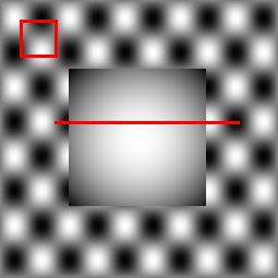
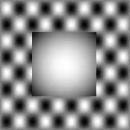
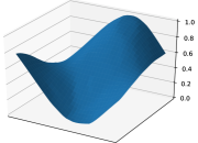
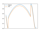
original image	$\mathop{\rm TGV}\nolimits_{\alpha}^{2}$-denoising	$\mathop{\rm TGV}\nolimits_{\alpha}^{2}$ surface plot	$\mathop{\rm TGV}\nolimits_{\alpha}^{2}$ line plot
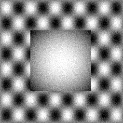
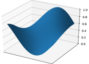
noisy image	$\mathop{\rm TGV}\nolimits_{\alpha}^{3}$-denoising	$\mathop{\rm TGV}\nolimits_{\alpha}^{3}$ surface plot	$\mathop{\rm TGV}\nolimits_{\alpha}^{3}$ line plot

Figure 12: Comparison of second- and third-order TGV for denoising for a piecewise smooth noisy image (PSNR: $26.0$dB). The red lines in the original image indicate the areas used in the line and surface plots. A close look on these plots reveals piecewise-linearity defects of $\mathop{\rm TGV}\nolimits^{2}_{\alpha}$, while the $\mathop{\rm TGV}\nolimits^{3}_{\alpha}$ reconstruction yields a better approximation of smooth structures and an improved PSNR ($\mathop{\rm TGV}\nolimits_{\alpha}^{2}$: $40.7$dB, $\mathop{\rm TGV}\nolimits_{\alpha}^{3}$: $42.3$dB). Note that in the line plots, the value $0.05$ was subtracted from the $\mathop{\rm TGV}\nolimits$-denoising results in order to prevent the respective plots from significantly overlapping with the plots of the original data.

Another problem class is image deblurring which can be considered as a standard test problem for the ill-posed inversion of linear operators in imaging. Pick a blurring kernel $k\in L^{\infty}(\Omega_{0})$ with bounded domains $\Omega_{0},\Omega^{\prime}\subset\mathbf{R}^{d}$ such that $\Omega^{\prime}-\Omega_{0}\subset\Omega$. Then, $K:L^{1}(\Omega)\rightarrow L^{2}(\Omega^{\prime})$ given by

$$(Ku)(x)=\int_{\Omega_{0}}u(x-y)k(y)\ \mathrm{d}{y},\quad x\in\Omega^{\prime}$$

is well-defined, linear and continuous. Consequently, by Theorems 2.11, 2.14 and Proposition 5.17,

$$\min_{u\in L^{p}({\Omega})}\ \frac{1}{2}\int_{\Omega^{\prime}}{|{(u\ast k)(x)-f(x)}|}^{2}\ \mathrm{d}{x}+\mathcal{R}_{\alpha}(u),$$

for $1<p\leq d/(d-1)$ and $\mathcal{R}_{\alpha}\in\{\alpha\mathop{\rm TV}\nolimits,\mathop{\rm TGV}\nolimits_{\alpha}^{2}\}$ admits a solution that stably depends on the data $f\in L^{2}({\Omega^{\prime}})$, which we assume to be a noise-contaminated image blurred by the convolution operator $K$. A numerical solution can again be obtained with the framework described in Section 6 and a comparison of the two choices of $\mathcal{R}_{\alpha}$ for a test image can be found in Figure 13. We can observe that both $\mathop{\rm TV}\nolimits$ and $\mathop{\rm TGV}\nolimits_{\alpha}^{2}$ are able to remove noise and blur from the image, however, the $\mathop{\rm TV}\nolimits$ reconstruction suffers from staircasing artefacts which are not present with $\mathop{\rm TGV}\nolimits_{\alpha}^{2}$.

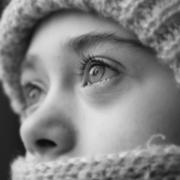
$u_{\mathrm{orig}}$	$f$
$u_{\mathop{\rm TV}\nolimits}$	$u_{\mathop{\rm TGV}\nolimits_{\alpha}^{2}}$

Figure 13: Deconvolution example. The original image $u_{\mathrm{orig}}$ [91] has been blurred and contaminated by noise resulting in $f$. The images $u_{\mathop{\rm TV}\nolimits}$ and $u_{\mathop{\rm TGV}\nolimits_{\alpha}^{2}}$ are the regularised solutions recovered from $f$.

7.2 Compressed sensing

The next problem we would like to discuss is compressive sampling with total variation and total generalised variation [27]. More precisely, we aim at reconstructing a single-channel image from ‘single-pixel camera’ data [77], an inverse problem with finite-dimensional data space. Here, an image is not observed directly but only the accumulated grey values over finitely many random pixel patterns are sequentially measured by one sensor, the ‘single pixel’. This can be modelled as follows. For a bounded Lipschitz image domain $\Omega\subset\mathbf{R}^{2}$, let the measurable sets $E_{1},\ldots,E_{M}\subset\Omega$ be the collection of random patterns where each $E_{m}$ is associated with the $m$-th measurement. The image $u$ is then determined by solving the inverse problem

$$Ku=f\qquad\mbox{where}\qquad(Ku)_{m}=\int_{E_{m}}u\ \mathrm{d}{x}\quad\mbox{for}\quad m=1,\ldots,M$$

and $f\in\mathbf{R}^{M}$ is the measurement vector, i.e., each $f_{m}$ is the output of the sensor for the pattern $E_{m}$. As the set of $u$ solving this inverse problem is an affine space with finite codimension, the compressive imaging approach assumes that the image $u$ is sparse in a certain representation which is usually translated into the discrete total variation $\mathop{\rm TV}\nolimits(u)$ being small. A way to reconstruct $u$ from $f$ is then to solve

$$\min_{u\in\mathop{\rm BV}\nolimits(\Omega)}\ S_{f}(Ku)+\mathop{\rm TV}\nolimits(u),\qquad S_{f}(v)=\mathcal{I}_{\{{f}\}}(v).$$ (88)

In this context, also higher-order regularisers may be used as sparsity constraint. For instance, in [27], total generalised variation of order $2$ has numerically been tested:

$$\min_{u\in\mathop{\rm BV}\nolimits(\Omega)}\ S_{f}(Ku)+\mathop{\rm TGV}\nolimits_{\alpha}^{2}(u),\qquad S_{f}(v)=\mathcal{I}_{\{{f}\}}(v).$$ (89)

Figure 14 shows example reconstructions for real data according to discretized versions of (88) and (89). As supported by the theory of compressed sensing [53, 52], the image can essentially be recovered from a few single-pixel measurements. Here, TGV-minimisation helps to reconstruct smooth regions of the image such that in comparison to TV-minimisation, more features can still be recognised, in particular, when reconstructing from very few samples. Once again, staircasing artefacts are clearly visible for the TV-based reconstructions, a fact that recently was made rigorous in [29, 26].

$\mathop{\rm TV}\nolimits$-based compressive imaging reconstruction
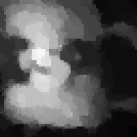
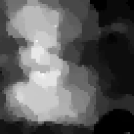
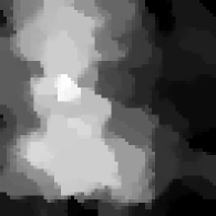
$768$ samples	$384$ samples	$256$ samples	$192$ samples
$\mathop{\rm TGV}\nolimits^{2}$-based compressive imaging reconstruction
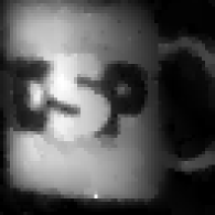
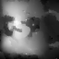
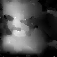
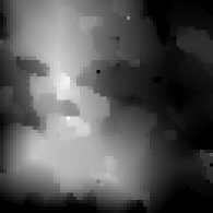
$768$ samples	$384$ samples	$256$ samples	$192$ samples

Figure 14: Example for $\mathop{\rm TV}\nolimits$/$\mathop{\rm TGV}\nolimits^{2}$ compressive imaging reconstruction for real single-pixel camera data [156]. Top: $\mathop{\rm TV}\nolimits$-based reconstruction of a $64\times 64$ image from 18.75%, 9.375%, 6.25% and 4.6875% of the data (from left to right). Bottom: $\mathop{\rm TGV}\nolimits^{2}$-based reconstruction obtained from the same data. Figure taken from [27]. Reprinted by permission from Springer Nature.

7.3 Optical flow and stereo estimation

Another important fundamental problem in image processing and computer vision is the determination of the optical flow [109] of an image sequence. Here, we consider this task for two consecutive frames $f_{0}$ and $f_{1}$ in a sequence of images. This is often modelled by minimising a possibly joint discrepancy $S_{f_{0},f_{1}}\bigl{(}u(0),u(1)\bigr{)}$ for $u:[0,1]\times\Omega\to\mathbf{R}$ subject to the optical flow constraint $\frac{\partial u}{\partial t}+\nabla u\cdot v=0$, see, for instance, [24]. Here, $v:[0,1]\times\Omega\to\mathbf{R}^{d}$ is the optical flow field that shall be determined. In order to deal with ill-posedness, ambiguities as well as occlusion, the vector field $v$ needs to be regularised by a penalty term. This leads to the PDE-constrained problem

$$\min_{u,v}\ S_{f_{0},f_{1}}\bigl{(}u(0),u(1)\bigr{)}+\mathcal{R}_{\alpha}(v)\qquad\mbox{subject to}\qquad\frac{\partial u}{\partial t}+\nabla u\cdot v=0,$$

where $\mathcal{R}_{\alpha}$ is a suitable convex regulariser for vector field sequences. Usually, $S_{f_{0},f_{1}}$ is chosen such that the initial condition $u(0)$ is fixed to $f_{0}$, for instance, $S_{f_{0},f_{1}}(u_{0},u_{1})=\mathcal{I}_{\{{f_{0}}\}}(u_{0})+\frac{1}{2}\|{u_{1}-f_{1}}\|_{2}^{2}$, see [102, 24, 117, 63].

In many approaches, this problem is reformulated to a correspondence problem. This means, on the one hand, replacing the optical flow constraint by the displacement introduced by a vector field $v_{0}:\Omega\to\mathbf{R}^{2}$, i.e., $u(0)=u_{0}$ and $u(1)=u_{0}\circ(\mathop{\rm id}\nolimits+v_{0})$. The image $u_{0}:\Omega\to\mathbf{R}$ is either prespecified or subject to optimisation. For instance, choosing again $S_{f_{0},f_{1}}(u_{0},u_{1})=\mathcal{I}_{\{{f_{0}}\}}(u_{0})+\frac{1}{2}\|{u_{1}-f_{1}}\|_{2}^{2}$ leads to the classical correspondence problem

$$\min_{v_{0}}\ \frac{1}{2}\|{f_{0}\circ(\mathop{\rm id}\nolimits+v_{0})-f_{1}}\|_{2}^{2}+\mathcal{R}_{\alpha}(v_{0}),$$

see, for instance, [109], which uses the square of the $H^{1}$-seminorm as a regulariser. On the other hand, other approaches have been considered for the discrepancy (and regularisation), see [47, 194]. In this context, a popular concept is the census transform [193] that describes the local relative behaviour of an image and is invariant to brightness changes. For an image $f:\Omega\to\mathbf{R}$, measurable patch $\Omega^{\prime}\subset\mathbf{R}^{2}$ and threshold $\varepsilon>0$, it is defined as

$$C_{f}:\Omega\times\Omega^{\prime}\to\{{-1,0,1}\},\quad C_{f}(x,y)=\left\{\begin{array}[]{cl}\mathop{\rm sgn}\nolimits\bigl{(}f(x+y)-f(x)\bigr{)}&\mbox{if}\ x,x+y\in\Omega\ \mbox{and}\\ &\ \ {|{f(x+y)-f(x)}|}>\varepsilon,\\ 0&\mbox{else}.\end{array}\right.$$

Here, one usually sets $u_{0}=f_{0}$ and $u_{1}=f_{1}$ such that the discrepancy only depends on the vector field $v_{0}$, such as, for instance,

$$S_{f_{0},f_{1}}(v_{0})=\int_{\Omega}\int_{\Omega^{\prime}}\min\bigl{(}1,\bigl{|}{C_{f_{0}}(x,y)-C_{f_{1}\circ(\mathop{\rm id}\nolimits+v_{0})}(x,y)}\bigr{|}\bigr{)}\ \mathrm{d}{y}\ \mathrm{d}{x},$$

leading to the optical-flow problem

$$\min_{v_{0}}\ S_{f_{0},f_{1}}(v_{0})+\mathcal{R}_{\alpha}(v_{0}),$$

see, for instance, [136, 187]. A closely related problem is stereo estimation which can also be modelled as a correspondence problem. In this context, $f_{0}$ and $f_{1}$ constitute a stereo image pair, for instance, $f_{0}$ being the left image and $f_{1}$ being the right image. The stereo information is then usually reflected by the disparity which describes the displacement of the right image with respect to the left image. This corresponds to setting the vertical component of the displacement field $v_{0}$ to zero, for instance, $(v_{0})_{2}=0$. Census-transform based discrepancies are also used for this task [151], leading to the stereo-estimation model

$$\min_{w_{0}}\ S_{f_{0},f_{1}}\bigl{(}(w_{0},0)\bigr{)}+\mathcal{R}_{\alpha}(w_{0})$$ (90)

with a suitable convex regulariser $\mathcal{R}_{\alpha}$ for scalar disparity images.

Both optical flow and stereo estimation are non-convex due to the non-convex data terms and require dedicated solution techniques. One possible approach is to smooth the discrepancy functional such that is becomes (twice) continuously differentiable, and approximate it, for each $x\in\Omega$, by either first or second-order Taylor expansion. For the latter case, if one also projects the pointwise Hessian to the positive semi-definite cone, one arrives at the convex problem

$$\min_{v}\ \int_{\Omega}S(v_{0})+\nabla S(v_{0})\cdot(v-v_{0})+\frac{1}{2}\mathop{\rm proj}\nolimits_{S^{+}}\bigl{(}\nabla^{2}S(v_{0})\bigr{)}(v-v_{0})\cdot(v-v_{0})\ \mathrm{d}{x}+\alpha\mathcal{R}(v),$$

where $v_{0}$ is the base vector field for the Taylor expansion and $\mathop{\rm proj}\nolimits_{S^{+}}:S^{2\times 2}\to S^{2\times 2}_{+}$ denotes the orthogonal projection to the cone of positive semi-definite matrices $S^{2\times 2}_{+}$. Besides classical regularisers such as the $H^{1}$-seminorm, the total variation has been chosen [191], i.e., $\mathcal{R}_{\alpha}=\alpha\mathop{\rm TV}\nolimits$, which allows the identification of jumps in the displacement field associated with object boundaries. The displacement field is, however, piecewise smooth such that $\mathop{\rm TGV}\nolimits_{\alpha}^{2}$ turns out to be advantageous. Further improvements can be achieved by non-local total generalised variation $\mathop{\rm NLTGV}\nolimits^{2}$, see [153], leading to sharper and more accurate motion boundaries, see Figure 15. For stereo estimation, a similar approach using first-order Taylor expansion and image-driven total generalised variation $\mathop{\rm ITGV}\nolimits_{\alpha}^{2}$ also yields very accurate disparity images [151].

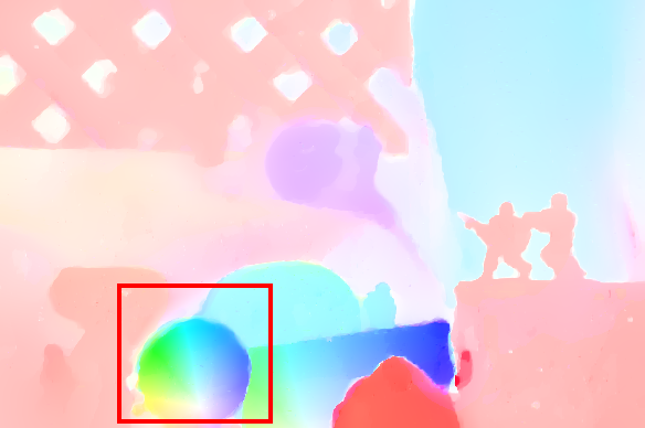
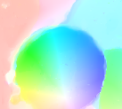
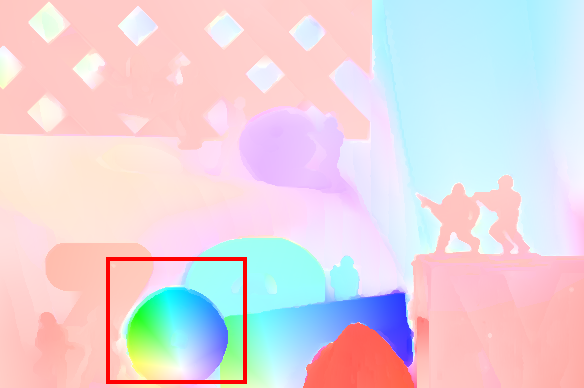
(a)	(b)	(c)	(d)

Figure 15: Example for higher-order approaches for optical flow determination. (a) An optical flow field obtained on a sample dataset from the Middlebury benchmark [11] using a $\mathop{\rm TGV}\nolimits_{\alpha}^{2}$ regulariser. (b) An enlarged detail of (a). (c) The optical flow field obtained by a $\mathop{\rm NLTGV}\nolimits^{2}$ regulariser. (d) An enlarged detail of (c). Images taken from [153]. Reprinted by permission from Springer Nature.

A different concept for solving the non-convex optical flow/stereo estimation problem is functional lifting [4, 55]. For the stereo estimation problem, this means to recover the characteristic function of the subgraph of the disparity image, i.e., $\chi_{\{{t\leq w_{0}}\}}$. Assume that the discrepancy for the disparity $w_{0}$ can be written in integral form, i.e., $S_{f_{0},f_{1}}(w_{0})=\int_{\Omega}g\bigl{(}x,w_{0}(x)\bigr{)}\ \mathrm{d}{x}$ with a suitable $g:\Omega\times\mathbf{R}\to\mathbf{R}$ that is possibly non-convex with respect to the second argument. If $w_{0}$ is of bounded variation, then $\chi_{\{{t\leq w_{0}}\}}$ is also of bounded variation and the weak derivative with respect to $x$ and $t$, respectively, are Radon measures. Denoting by $v_{x}$ and $v_{t}$ the respective components of a vector, i.e., $v=(v_{x},v_{t})\in\mathbf{R}^{2}\times\mathbf{R}$, these derivatives satisfy the identity $\frac{\partial}{\partial t}\chi_{\{{t\leq w_{0}}\}}=\bigl{(}\frac{\nabla\chi_{\{{t\leq w_{0}}\}}}{{|{\nabla\chi_{\{{t\leq w_{0}}\}}}|}}\bigr{)}_{t}{|{\nabla\chi_{\{{t\leq w_{0}}\}}}|}$ as well as $\nabla_{x}\chi_{\{{t\leq w_{0}}\}}=\bigl{(}\frac{\nabla\chi_{\{{t\leq w_{0}}\}}}{{|{\nabla\chi_{\{{t\leq w_{0}}\}}}|}}\bigr{)}_{x}{|{\nabla\chi_{\{{t\leq w_{0}}\}}}|}$. The discrepancy term can then be written in the form

$$S_{f_{0},f_{1}}\bigl{(}(w_{0},0)\bigr{)}=\int_{\Omega\times\mathbf{R}}g\ \mathrm{d}{\Bigl{|}{\frac{\partial}{\partial t}\chi_{\{{t\leq w_{0}}\}}}\Bigr{|}}$$

which is convex with respect to $\chi_{\{{t\leq w_{0}}\}}$. In many cases, regularisation functionals can also be written in terms of $\chi_{\{{t\leq w_{0}}\}}$, for instance, by the coarea formula,

$$\mathop{\rm TV}\nolimits(w_{0})=\int_{\Omega\times\mathbf{R}}\ \mathrm{d}{{|{\nabla_{x}\chi_{\{{t\leq w_{0}}\}}}|}},$$

which is again convex with respect to $\chi_{\{{t\leq w_{0}}\}}$. As the set of all $\chi_{\{{t\leq w_{0}}\}}$ is still non-convex, this constraint is usually relaxed to a convex set, for instance, to the conditions

$$u\in\mathop{\rm BV}\nolimits(\Omega\times\mathbf{R}),\quad 0\leq u\leq 1,\quad\lim_{t\to-\infty}u(t,\,\cdot\,)=\mathbf{1},\quad\lim_{t\to\infty}u(t,\,\cdot\,)=0,$$ (91)

where the limits have to be understood in a suitable sense. Then, the stereo problem (90) with total-variation regularisation can be relaxed to the convex problem

$$\min_{u\in\mathop{\rm BV}\nolimits(\Omega\times\mathbf{R})}\ \int_{\Omega\times\mathbf{R}}g\ \mathrm{d}{\Bigl{|}{\frac{\partial u}{\partial t}}\Bigr{|}}+\alpha\int_{\Omega\times\mathbf{R}}\ \mathrm{d}{{|{\nabla_{x}u}|}}\qquad\mbox{subject to}\ {(\ref{eq:functional_lifting_constraint})}.$$

Then, optimal solutions $u^{*}$ for the above problem yield minimizers of the original problem when thresholded, i.e., for $s\in{]{0,1}[}$, the function $\chi_{\{{s\leq u^{*}}\}}$ is the characteristic function of the subgraph of a $w_{0}$ that is optimal for (90) for the assumed discrepancy and total-variation regularisation [144].

Unfortunately, a straightforward adaptation of this strategy to higher-order total-variation-type regularisation functionals is not possible. For $\mathop{\rm TGV}\nolimits^{2}$, one can nevertheless benefit from the convexification approach. Considering the $\mathop{\rm TGV}\nolimits_{2}^{\alpha}$-regularised problem

$$\min_{w_{0}\in\mathop{\rm BV}\nolimits(\Omega),\ w\in\mathop{\rm BD}\nolimits(\Omega)}\ \int_{\Omega}g(x,w_{0}(x)\bigr{)}\ \mathrm{d}{x}+\alpha_{1}\int_{\Omega}\ \mathrm{d}{{|{\nabla w_{0}-w}|}}+\alpha_{0}\int_{\Omega}\ \mathrm{d}{{|{\mathcal{E}w}|}},$$ (92)

one sees that the problem is convex in $w$ and minimisation with respect to $w_{0}$ can still be convexified by functional lifting. For fixed $w$, the latter leads to

$$\begin{array}[]{rl}\displaystyle\min_{u\in\mathop{\rm BV}\nolimits(\Omega\times\mathbf{R})}\ \int_{\Omega}g\ \mathrm{d}{\Bigl{|}{\frac{\partial u}{\partial t}}\Bigr{|}}+\alpha_{1}\sup\ \Bigl{\{}\int_{\Omega\times\mathbf{R}}u\mathop{\rm div}\nolimits\varphi\ \mathrm{d}{x}\ \Bigl{|}&\displaystyle\varphi\in\mathcal{C}_{\mathrm{c}}^{\infty}({\Omega,\mathbf{R}^{2}\times\mathbf{R}}),{|{\varphi_{x}(x,t)}|}\leq 1,\\ &\varphi_{x}(x,t)\cdot w(x)\leq\varphi_{t}(x,t)\ \mbox{a.e.~{}in}\ \Omega\times\mathbf{R}\Bigr{\}}\\ \mbox{subject to}\ {(\ref{eq:functional_lifting_constraint})},\end{array}$$

which is again convex and whose solutions can again be thresholded to yield a $w_{0}^{*}$ that is optimal with respect to $w_{0}$ for a fixed $w$. Alternating minimisation then provides a robust solution strategy for (92) based on convex optimisation [154], see Figure 16 for an example.

(a)
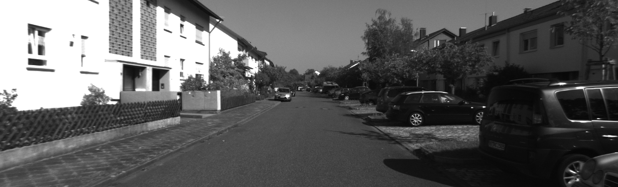
(b)

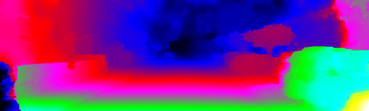
Figure 16: Total-generalised-variation-regularised stereo estimation based on functional lifting and convex optimisation for an image pair of the KITTI dataset [90]. (a) The reference image. (b) The disparity image obtained with $\mathop{\rm TGV}\nolimits^{2}$-regularisation [154]. Images taken from [152].

In this context, algorithms realising functional lifting strategies for TV and TGV regularisation have recently further been refined, for instance, in order to lower the computational complexity associated with the additional space dimension introduced by the lifting, see, e.g. [134, 180].

7.4 Image and video decompression

Pixelwise representations of image or image sequence data require, on the one hand, a large amount of digital storage but contain, on the other hand, enough redundancy to enable compression. Indeed, most digitally stored images and image sequences, e.g., on cameras, mobile phones or the world-wide web are compressed. Commonly-used lossy compression standards such as JPEG, JPEG2000 for images and MPEG for image sequences, however, suffer from visual artefacts in decompressed data, especially for high compression rates.

Those artefacts result from errors in the compressed data due to quantisation, which is not accounted for in the decompression procedure. These errors, however, can be well described using the data that is available in the compressed file and in particular, precise bounds on the difference of the available data and the unknown, ground truth data can be obtained. This observation motivates a generic approach for an improved decompression of such compressed image or video data, which consists of minimising a regularisation functional subject to these error bounds, see for instance [198, 5, 31] for TV-based works in this context. Following this generic approach, we present here a TGV-based reconstruction method (see [33, 34]) that allows for a variational reconstruction of still images from compressed data that is directly applicable to the major image compression standards such as JPEG, JPEG2000 or the image compression layer of the DjVu document compression format [107]. A further extension of this model to the decompression of MPEG encoded video data will be addressed afterwards.

The underlying principle of a broad class of image and video compression standards, and in particular of JPEG and JPEG 2000 compression, is as follows: First, a linear transformation is used to transform the image data to a different representation where information that is more and less important for visual image quality is well separated. Then, a weighted quantisation of this data (according to its expected importance for visual image quality) is carried out and the quantised data (together with information that allows to obtain the quantisation accuracy) is stored. Thus, defining $K$ to be the linear transformation used in the compression process and $D$ to be a set of admissible, transformed image data that can be obtained using the information available in the compressed file, decompression amounts to finding an image $u$ such that $Ku\in D$. Using the TGV functional to regularise this compression procedure and considering colour images $u:\Omega\rightarrow\mathbf{R}^{3}$, we arrive at the following minimisation problem:

$$\min_{u\in L^{2}(\Omega,\mathbf{R}^{3})}\ \mathcal{I}_{U_{D}}(u)+\mathop{\rm TGV}\nolimits_{\alpha}^{k}(u),\qquad U_{D}=\{{u\in L^{2}(\Omega,\mathbf{R}^{3})}\ \bigl{|}\ {Ku\in D}\}$$ (93)

where $K:L^{2}(\Omega,\mathbf{R}^{3})\rightarrow\ell^{2}$ is an analysis operator related to a Riesz basis of $L^{2}(\Omega,\mathbf{R}^{3})$, and a Frobenius-norm-type coupling of the colour channels is used in $\mathop{\rm TGV}\nolimits$, see Subsection 5.3. The coefficient dataset $D\subset\ell^{2}$ reflects interval restrictions on the coefficients, i.e., is defined as $D=\{{v\in\ell^{2}}\ \bigl{|}\ {v_{n}\in J_{n}\ \mbox{for all}\ n\in\mathbf{N}}\}$ for $\{{J_{n}}\}$ a family of closed intervals. In case $D$ is bounded, well-posedness of this approach can be obtained via a direct extension of Proposition 5.17 to $\mathbf{R}^{3}$-valued functions, which in particular requires a multi-channel version of the Poincaré inequality for TGV as in Proposition 5.15. The latter can straightforwardly be obtained by equivalence of norms in finite dimensions, see for instance [27, 33]. Beyond that, existence of a solution to (93) can be guaranteed also in case of a non-coercive discrepancy when arbitrarily many of the intervals $J_{n}$ are unbounded, provided that only finitely many of them are half-bounded, i.e., are the form $J_{n}={]{-\infty,c_{n}}]}$ or $J_{n}={[{c_{n},\infty}[}$ for $c_{n}\in\mathbf{R}$, see [33]. In compression, half-bounded intervals would correspond to knowing only the sign but not the precision of the respective coefficient, a situation which does not occur in JPEG, JPEG2000 and DjVu. Thus, in all relevant applications, all intervals are either bounded or all of $\mathbf{R}$, and hence, solutions exist. Further, under the assumption that all but finitely many intervals have a width that is uniformly bounded from below, again an assumption which holds true in all anticipated applications, optimality conditions for (93) can be obtained.

In the application to JPEG decompression, colour images are processed in the YCbCr colour space and the basis transformation operator $K$ corresponds to a colour subsampling followed by a block- and channel-wise discrete cosine transformation, which together can be expressed as Riesz-basis transform. The interval sequence $\{{J_{n}}\}$ can be obtained using a quantisation matrix that is available in the encoded file and each interval $J_{n}$ is bounded.

In the application to JPEG2000 decompression, again the YCbCr colour space is used and $K$ realises a colour-component-wise biorthogonal wavelet transform using Le Gall 5/3 or CDF 9/7 wavelets as defined in [64, Table 6.1 and Table 6.2]. Obtaining bounds on the precision of the wavelet coefficients is more involved than with JPEG (see [33, Section 4.3]), but can be done by studying the bit truncation scheme of JPEG2000 in detail. As opposed to JPEG, however, the intervals $J_{n}$ might either be bounded or unbounded.

A third application of the model (93) is a variational decompression of the image layers of a DjVu compressed document. DjVu [99] is a storage format for digital documents. It encodes document pages via a separation into fore- and background layers as well as a binary switching mask, where the former are encoded using a lossy, transform-based compression and the latter using a dictionary-based compression. While the binary switching mask typically encodes fine details such as written text, the fore- and background layer encode image data, which again suffers from compression artefacts that can be reduced via variational decompression. Here, the extraction of the relevant coefficient data together with error bounds has to account for the particular features of the DjVu compression standard (we refer to [107] and its supplementary material for a detailed description and software that extracts the relevant data from DjVu compressed files), but the overall model for the image layers is again similar to the one of JPEG and JPEG2000 decompression. In particular, encoding of the fore- and background layer can be modelled with the operator $K$, in this case corresponding to a colour-component-wise wavelet transformation using the Dubuc–Deslauriers–Lemire (DDL) (4, 4) wavelets [74], and the data intervals $J_{n}$, which are again either bounded or all of $\mathbf{R}$.

In all of the above applications, a numerical solution of the corresponding particular instance of the minimisation problem (93) can be obtained using the primal-dual framework [34] as described in Section 6 (see [34] for details). We refer to Figure 17 for exemplary results using second-order TGV regularisation. Regarding the implementation, relevant differences arise depending on whether the projection onto the dataset $U_{D}$ can be carried out explicitly or not, the latter requiring a dualization of this constraint and an additional dual variable. Only in the application to JPEG decompression, this projection is explicit due to orthonormality of the cosine transform and the particular structure of the colour subsampling operator. This has the particular advantage that, at any iteration of the algorithm, the solution is feasible and one can, for instance, apply early stopping techniques to obtain already quite improved decompressed images in a computationally cheap way.

Variational MPEG decompression.

The MPEG video compression standard builds on JPEG compression for storing frame-wise image data, but incorporates additional motion prediction and correction steps which can significantly reduce storage size of video data. In MPEG-2 compression, which is a tractable blueprint for the MPEG compression family, video data is processed as subsequent groups of pictures (typically 12-15 frames) which can be handled separately. In each group of pictures, different frame types (I, P and B frames) are defined, and, depending to the frame type, image data is stored by using motion prediction and correction followed by a JPEG-type compression of the corrected data. Similar to JPEG compression, colour images are processed in the YCbCr colour space and additional subsampling of colour components is allowed.

While these are the main features of a typical MPEG video encoder, as usual for most compression standards, the MPEG standard defines the decompression procedure rather than compression. Hence, since compression might differ for different encoders, we build a variational model for MPEG decompression that works with a decoding operator (see [35] for more details on MPEG and the model): Using the information (in particular motion correction vectors and quantisation tables) that is stored in the MPEG compressed files, we can define a linear operator $K$ that maps encoded, motion corrected cosine-transform coefficient data to (colour subsampled) video data. Furthermore, bounds on the coefficient data can be obtained. Using a second operator $S$ to model colour subsampling and choosing a right-inverse $\hat{S}$, MPEG decompression amounts to finding a video $u$ such that

$$u=s+\hat{S}Kv,$$

where $v\in D$ with $D$ being the admissible set of cosine coefficient data, and $s\in\ker(S)$ compensates for the colour upsampling of $\hat{S}$. Incorporating the infimal-convolution of second-order spatio-temporal TGV functionals as regularisation for video data (see Subsection 5.3 and [35, 108]), decompression then amounts to solve

$$\min_{v\in D,\ s\in\ker(S)}\mathop{\rm ICTGV}\nolimits(s+\hat{S}Kv).$$

Again, the minimisation problem can be solved using duality-based convex optimisation methods as described in Section 6 and we refer to Figure 18 for a comparison of standard MPEG-2 decompression and the result obtained with this model.

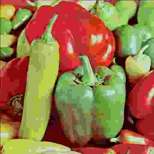
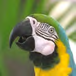
Figure 17: Example of variational image decompression. Standard (left column) and TGV-based (right column) decompression for a JPEG image (top row) compressed to 0.15 bits-per-pixel (bpp), a JPEG2000 image (middle row) compressed to 0.3 bpp, and a DjVu-compressed document page (bottom row) with close-ups. Results from [34] (rows 1–2) and [107] (bottom row).

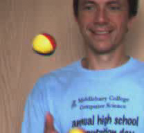
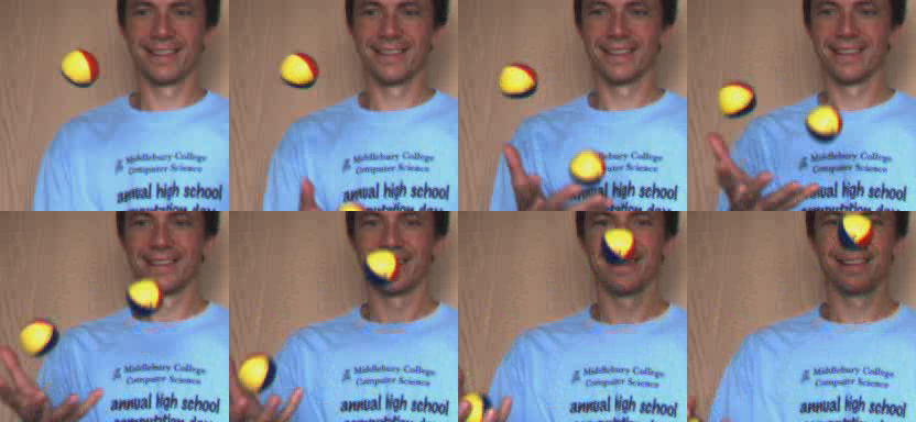
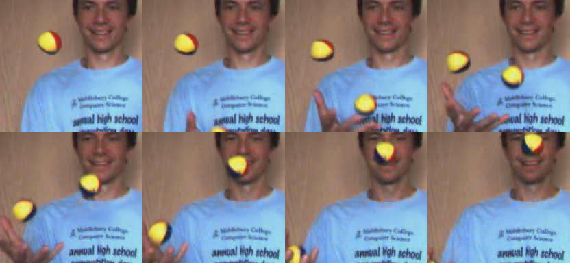
Figure 18: Example of variational MPEG decompression. Standard (top row) and ICTGV-based (bottom row) decompression of the Juggler image sequence from [11]. On the left, the second frame (P-frame) is shown in detail while on the right, all 8 frames are depicted. Figure taken from [35]. Reprinted by permission from Springer Nature.

8 Applications in medical imaging and image reconstruction

8.1 Denoising of dual-energy computed-tomography (CT) data

Since its development in the 1970s, computed X-ray tomography (CT) became a standard tool in medical imaging. As CT bases on X-rays, the health risks associated with ionising radiation is certainly a drawback of this imaging technique. Further, the acquired images do in general not allow to differentiate objects with the same density. For the former point, a low radiation dose is an important goal, being, of course in conflict with the demand of a high signal-to-noise ratio (SNR). Regarding the differentiation of objects with the same density [87, 114], a recently developed approach bases on an additional dataset from a second X-ray source (typically placed in a 90 degree offset) which possess a different spectrum (or energy) compared to the standard X-ray emitter in CT, the dual-energy CT device, see Figure 19 (a).

Objects of different material having the same response for one X-ray source may admit a different response for the second source, making a differentiation possible. A relevant application of this principle is, for instance, the quantification of contrast agent concentration. Adjusting a dual-energy CT device such that normal tissue is insensitive for both X-ray sources and sensitive for an administered contrast agent allows to infer its concentration from the difference of the two acquired images, see Figure 19 (b). This may be useful, for instance, for recognising perfusion deficits and thus aid the diagnosis of, e.g., pulmonary embolism in the lung [130]. However, due to low doses for the dual-energy CT scan as well as a limited sensitivity with respect to the contrast agent, the difference image can be noisy and denoising is required in order to obtain a meaningful interpretation, see Figure 19 (c).

In the following, a variational denoising approach is derived that takes the structure of the problem into account. First, let $A_{0}$ and $B_{0}$ be the noisy CT-reconstructions associated with the respective X-ray source. Then, as the difference image contains the relevant information, we would like to impose regularity on the difference image $A-B$ as well as a “base” image $B$ instead of penalising each image separately. As we may assume that the contrast agent concentration as well as the density is piecewise smooth, is admits a low total generalised variation, and hence, we choose this functional as a penalty, for instance of second order. Furthermore, as the results should be usable for a quantification, we have to account for that and therefore choose an $L^{1}$-fidelity term as this is known to possess desirable contrast-preservation properties in conjunction with $\mathop{\rm TV}\nolimits$ and $\mathop{\rm TGV}\nolimits$ [61, 38]. In total, this leads to the variational problem

$$\min_{(A,B)\in L^{1}({\Omega})^{2}}\ \|{A-A_{0}}\|_{1}+\|{B-B_{0}}\|_{1}+\mathop{\rm TGV}\nolimits^{2}_{\alpha}(B)+\mathop{\rm TGV}\nolimits_{\alpha^{\prime}}^{2}(A-B)$$

where $A_{0},B_{0}\in L^{1}({\Omega})$ is given and $\alpha=(\alpha_{0},\alpha_{1})$ as well as $\alpha^{\prime}=(\alpha_{0}^{\prime},\alpha_{1}^{\prime})$ are positive regularisation parameters. Having the application in mind, the domain $\Omega$ is typically a bounded three-dimensional domain with Lipschitz boundary. Then, existence of minimizers can be obtained using the tools from Section 5, see Proposition 5.17, which nevertheless requires some straightforward adaptations. Due to the lack of strict convexity, however, the solutions might be non-unique. Further, numerical algorithms can be developed along the lines of Section 6, for instance, a primal-dual algorithm as outlined in Subsection 6.2. In case of non-uniqueness, the minimisation procedure “chooses” one solution in the sense that it converges to one element of the solution set, such that variational model and optimisation algorithm cannot clearly be separated and other results might be possible using different optimisation algorithms.

Figure 19 (d) shows denoising results for the primal-dual algorithm, where a clear improvement of image quality for the difference image in comparison to Figure 19 (c) can be observed. In particular, the total generalised variation model is suitable to recover the smooth distribution of the contrast agent within the lung, including the perfusion deficit region, as well as the discontinuities induced by bones, vessels, etc. Further, one can see that the dedicated modelling of the problem as a denoising problem for a difference image based on two datasets turns out to be beneficial. A denoising procedure that only depends on the noisy difference image would not allow for such an improvement of image quality.

(a)

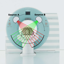
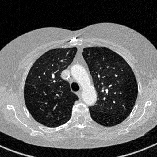
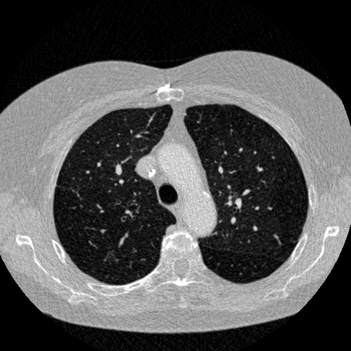
(b)

(c)

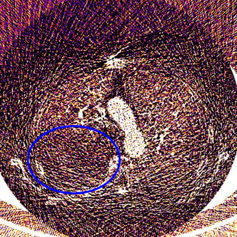
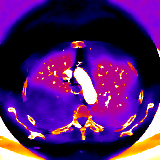
(d)

Figure 19: Example of $L^{1}$-$\mathop{\rm TGV}\nolimits^{2}$ denoising for dual energy computed tomography. (a) A schematic of a dual-energy CT device. (b) A pair of (reconstructed) dual-energy CT images. (c) A noisy difference image with marked perfusion deficit region. (d) Difference image of the TGV-denoised dataset (3D denoising, only one slice is shown).

8.2 Parallel reconstruction in magnetic resonance imaging

Magnetic resonance imaging (MRI) is a tomographic imaging technique that is heavily used in medical imaging and beyond. It builds on an interplay of magnetic fields and radio-frequency pulses, which allows for localised excitation and, via induction of current in receiver coils, for a subsequent measurement of the proton density inside the object of interest [46]. In the standard setting, MRI delivers qualitative images visualising the density of hydrogen protons, e.g., inside the human body. Its usefulness is in particular due to an excellent soft tissue contrast (as opposed to computed tomography) and a high spatial resolution of MR images. The trade-off, in particular for the latter, is the long measurement time, which comes with obvious drawbacks such as patient discomfort, limitations on patient throughput and imaging artefacts resulting from temporally inconsistent data due to patient motion.

Subsampled data acquisition and parallel imaging [178, 148, 96] (combined with appropriate reconstruction methods) are nowadays standard techniques to accelerate MRI measurements. As the data in an MR experiment is acquired sequentially, a reduced number of measurements directly implies a reduced measurement time, however, in order to maintain the same image resolution, the resulting lack of data needs to be compensated for by other means. Parallel imaging achieves this to some extent by using not a single but multiple measurement coils and combining the corresponding measured signals for image reconstruction. On top of that, advanced mathematical reconstruction methods such as compressed sensing techniques [21, 131] or, more general, variational reconstruction have been shown to allow for a further, significant reduction of measurement time with a negligible loss of image quality.

In this context, transform-based regularisation techniques [131, 132] and derivative-based techniques [21, 120] are among the most popular approaches. More recently, also learning-based methods building on the structure of variational approaches have become very popular [100, 149]. Here, we focus on variational regularisation approaches with first- and higher-order derivatives. To this aim, we first deal with the forward model of parallel, static MR imaging.

In a standard setting, the MR measurement process can be modelled as measuring Fourier coefficients of the unknown image. In order to include measurements from multiple coils, spatially varying sensitivity profiles of these coils also need to be included in the forward model via a pointwise multiplication in image space. Subsampled data acquisition then corresponds to measuring the Fourier coefficients only on a certain measurement domain in Fourier space, which is defined by a subsampling pattern. Let $c_{1},\ldots,c_{k}\in\mathcal{C}_{0}(\mathbf{R}^{d},\mathbf{C})$ be functions modelling some fixed coil sensitivity profiles for $k$ receiver coils, let $\sigma$ be a positive, finite Radon measure on $\mathbf{R}^{d}$ that defines the sampling pattern, and let $\Omega\subset\mathbf{R}^{d}$ be a bounded Lipschitz domain that represents the image domain. Then, following the lines of [30], we define, for $p\in[1,\infty]$, the MR measurement operator $K:L^{p}({\Omega,\mathbf{C}})\rightarrow L^{2}_{\sigma}(\mathbf{R}^{d},\mathbf{C})^{k}$ as

$$(Ku)_{i}(\xi)=\widehat{c_{i}u}(\xi)=\frac{1}{(2\pi)^{d/2}}\int_{\mathbf{R}^{d}}c_{i}(x)u(x)\rme^{-\mathrm{i}\xi\cdot x}\ \mathrm{d}{x},\quad\xi\in\mathbf{R}^{d},$$ (94)

where we extend $u$ by zero to $\mathbf{R}^{d}$. Note that for each $u\in L^{p}({\Omega,\mathbf{C}})$, $Ku$ as a function on $\mathbf{R}^{d}$ is bounded and continuous which follows from

$$|(Ku)_{i}(\xi)|\leq\frac{\|c_{i}\|_{\infty}}{(2\pi)^{d/2}}\|u\|_{1}\leq C\frac{\|c_{i}\|_{\infty}}{(2\pi)^{d/2}}\|u\|_{p}.$$

Thus, since $\sigma$ is finite, $K$ indeed linearly and continuously maps into $L^{2}_{\sigma}({\mathbf{R}^{d},\mathbf{C}})$.

While here, we assume the coil sensitivities to be known (such that the forward model is linear), obtaining them prior to image reconstruction is non-trivial and we refer to [21, 165, 189, 184] for some existing methods. In the experiments discussed below, we followed the approach of [21] and employed, for each individual coil, a variational reconstruction with a quadratic regularisation on the derivative ($H^{1}$-regularisation) followed by the convolution with a smoothing kernel. For each coil, the sensitivity profile was then obtained by division with the sum-of-squares image (which is, despite its name, the pointwise square root of the sum of the squared modulus of the individual coil images).

A regularised reconstruction from MR measurement data $f\in L^{2}_{\sigma}({\mathbf{R}^{d},\mathbf{C}})^{k}$ can be obtained by solving

$$\min_{u\in L^{p}({\Omega,\mathbf{C}})}\ \frac{1}{2}\sum_{i=1}^{k}\|(Ku)_{i}-f_{i}\|_{2}^{2}+\mathcal{R}_{\alpha}(u),$$ (95)

where we test with both $\mathcal{R}_{\alpha}=\alpha\mathop{\rm TV}\nolimits$ and $\mathcal{R}_{\alpha}=\mathop{\rm TGV}\nolimits_{\alpha}^{2}$, in which case we can choose $1<p\leq d/(d-1)$. Note that well-posedness for (95) follows from Theorems 2.11, 2.14 in the case of TV and from Proposition 5.17 in the case of $\mathop{\rm TGV}\nolimits_{\alpha}^{2}$ (where straightforward adaptions are necessary to include complex-valued functions). Numerically, the optimisation problem can be solved using the algorithmic framework described in Section 6, where again, some modifications are necessary to deal with complex-valued images.

Figure 20 compares the results between these two choices of regularisation functionals and a conventional reconstruction based on direct Fourier inversion using non-uniform fast Fourier transform (NUFFT) [86] for different subsampling factors and a dataset for which a fully sampled ground truth is available. Undersampled 2D radial spin-echo measurements of the human brain were performed with a clinical 3T scanner using a receive-only 12 channel head coil. Sequence parameters were: $T_{R}=$ 2500 ms, $T_{E}=$ 50 ms, matrix size $256\times 256$, slice thickness 2 mm, in-plane resolution 0.78 mm$\times$0.78 mm. The sampling direction of every second spoke was reversed to reduce artefacts from off-resonances [22], and numerical experiments were performed using 96, 48 and 24 projections. As $\frac{\pi}{2}N$ projections ($402$ for $N=256$ in our case) have to be acquired to obtain a fully sampled dataset in line with the Nyquist criterion [18], this corresponds to undersampling factors of approximately 4, 8 and 16. The raw data was exported from the scanner, and image reconstruction was performed offline.

It can be seen that in particular at higher subsampling factors, variational, derivative-based reconstruction reduces artefacts stemming from limited Fourier measurements. Both TV and TGV perform well, while a closer look reveals that staircasing artefacts present with TV can be avoided using second-order TGV regularisation.

	NUFFT	TV	TGV
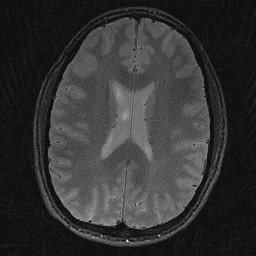
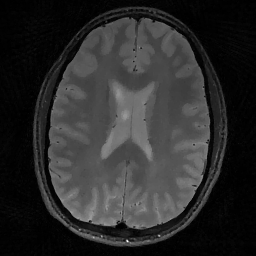
96
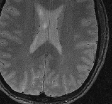
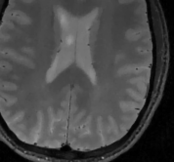
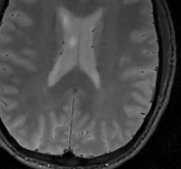
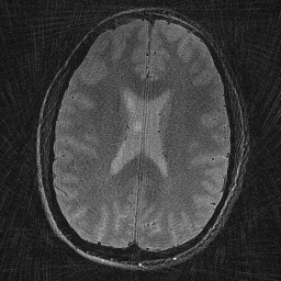
48
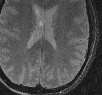
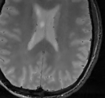
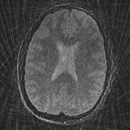
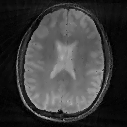
24

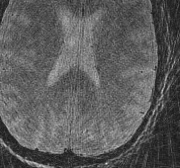
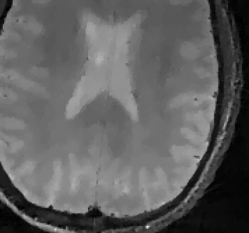
Figure 20: Parallel undersampling MRI of the human brain (256$\times$256 pixels) from 96, 48 and 24 radial projections (top, middle, bottom row). Left column: Conventional NUFFT reconstruction. Middle column: Reconstruction with TV regularisation. Right column: Reconstruction with $\mathop{\rm TGV}\nolimits^{2}$ regularisation. All reconstructed images are shown with a closeup of the lower right brain region.

8.3 Diffusion tensor imaging

Magnetic resonance imaging offers, apart from obtaining morphological images as outlined in Subsection 8.2, many other possibilities to acquire information about the imaged objects. Among these possibilities, diffusion tensor imaging (DTI) is one of the more recent developments. It aims at measuring the diffusion directions of water protons in each spatial point. The physical background is given by the Bloch–Torrey equation which describes the spatio-temporal evolution of magnetisation vector taking diffusion processes into account [182]. Based on this, diffusion-weighted imaging can be performed which uses dedicated MR sequences depending on a direction vector $q\in\mathbf{R}^{3}$ in order to obtain displacement information associated with that direction.

This leads to the following model. Assume that $\rho_{0}:\mathbf{R}^{3}\to\mathbf{R}$ is the proton density to recover and $\rho_{t}:\mathbf{R}^{3}\times\mathbf{R}^{3}\to\mathbf{R}$ is the function such that for each $x,x^{\prime}\in\mathbf{R}^{3}$, the value $\rho_{t}(x,x^{\prime})$ represents the probability of a proton moving from $x$ to $x^{\prime}$ during the time $t>0$. By applying a diffusion-sensitive sequence (such as, e.g., a pulsed-gradient spin echo [179]) associated with the vector $q\in\mathbf{R}^{3}$, one is able to measure in $k$-space as follows:

$$S(k,q)=\frac{1}{(2\pi)^{3}}\int_{\mathbf{R}^{3}}\rho_{0}(x)\mathrm{e}^{-\mathrm{i}k\cdot x}\int_{\mathbf{R}^{3}}\rho_{t}(x,x^{\prime})\mathrm{e}^{-\mathrm{i}q\cdot(x^{\prime}-x)}\ \mathrm{d}{x^{\prime}}\ \mathrm{d}{x},$$

where $k\in\mathbf{R}^{3}$, see [51, 66]. Note that in practice, also the coil sensitivity profile would influence the measurement as outlined in Subsection 8.2, however, for the sake of simplicity, we neglect this aspect in the following. Now, sampling $q$ across $\mathbf{R}^{3}$ would then, in principle, allow to recover the 6-dimensional function $u:(x,x^{\prime})\mapsto\rho_{0}(x)\rho_{t}(x,x^{\prime})$ by inverse Fourier transform, since $S(k,q)=(\mathcal{F}u)(k-q,q)$ for each $k,q\in\mathbf{R}^{3}$. The 6D-space spanned by the coordinates $k$ and $q$ is called $kq$-space. Assuming that for a fixed $q\in\mathbf{R}^{3}$, the $k$-space is fully sampled then allows to recover $f_{q}:\mathbf{R}^{3}\to\mathbf{C}$ by inverse Fourier transform, where

$$f_{q}(x)=\rho_{0}(x)\frac{1}{(2\pi)^{3/2}}\int_{\mathbf{R}^{3}}\rho_{t}(x,x^{\prime})\mathrm{e}^{-\mathrm{i}q\cdot(x^{\prime}-x)}\ \mathrm{d}{x^{\prime}}.$$

Obtaining and analysing $f_{q}$ for a coverage of the $q$-space is called $q$-space imaging which also is the basis of orientation-based analysis such as $q$-ball imaging [183]. However, as these techniques require too much measurement time in practice, one usually makes assumptions about the structure of $\rho_{t}$ in order to avoid the measurement of $f_{q}$ for too many $q$.

Along this line, the probably simplest model is to assume that for each $x$, $\rho_{t}(x,\,\cdot\,)$ follows a Gaussian distribution centred around $x$ with symmetric positive definite covariance matrix $2tD(x)\in S^{3\times 3}$, i.e.,

$$\rho_{t}(x,x^{\prime})=\frac{1}{\sqrt{(4\pi t)^{3}{|{\det D(x)}|}}}\mathrm{e}^{-\frac{1}{4t}(x^{\prime}-x)\cdot D(x)^{-1}(x^{\prime}-x)}.$$

For fixed $x\in\mathbf{R}^{3}$, this can be interpreted as the fundamental solution of the diffusion equation

$$\frac{\partial\rho}{\partial t}-\mathop{\rm div}\nolimits\bigl{(}D(x)\nabla_{x^{\prime}}\rho\bigr{)}=0\quad\mbox{in}\quad{]{0,\infty}[}$$

shifted by $x$ and evaluated at time $t$. The model for $\rho_{t}$ thus indeed reflects linear diffusion through a homogeneous medium. This makes sense as diffusion during the measurement process is usually orders of magnitudes smaller than the spatial scale one is interested in, but the homogeneity assumption might also be violated in case when microstructures are present. Nevertheless, with this assumption, in the above case of full $k$-space sampling, one gets

$$f_{q}(x)=\rho_{0}(x)\mathrm{e}^{-tq\cdot D(x)q}.$$ (96)

Clearly, for $q=0$, we have $f_{0}=\rho_{0}$, and assuming $\rho_{0}>0$ almost everywhere leads to the following pointwise equation that is linear in $D$:

$$D\cdot(q\otimes q)=-\frac{1}{t}\log\Bigl{(}\frac{f_{q}}{f_{0}}\Bigr{)}.$$

Hence, one can recover by $D$ by measuring $f_{0}$ and $f_{q_{1}},\ldots f_{q_{m}}$ for $q_{1},\ldots,q_{m}\in\mathbf{R}^{3}$ suitably chosen, i.e., such that in particular, $D$ is uniquely determinable from $D\cdot(q_{i}\otimes q_{i})$ for $i=1,\ldots,m$. In particular, one requires that the symmetric tensors $q_{1}\otimes q_{1},\ldots,q_{m}\otimes q_{m}$ span the space $\mathop{\rm Sym}\nolimits^{2}(\mathbf{R}^{3})$, meaning that $m$ must be at least $6$. Note that according to (96), $f_{q}$ must be real and non-negative, such that in practice, it suffices to reconstruct the absolute value of $f_{q}$, for instance, by computing the sum-of-squares image.

The inverse problem for $D$ can then be described as follows. Restricting the considerations to a bounded domain $\Omega\subset\mathbf{R}^{3}$ and letting $p\in[1,\infty]$ such that $g_{1},\ldots,g_{m}\in L^{p}({\Omega})$ where $g_{i}=-\frac{1}{t}\log(f_{q_{i}}/f_{0})$, we aim at solving

$$D\cdot(q_{i}\otimes q_{i})=g_{i}\quad\mbox{for}\quad i=1,\ldots,m,$$ (97)

for $D\in L^{p}({\Omega,\mathop{\rm Sym}\nolimits^{2}(\mathbf{R}^{3})})$. It is easy to see that this problem is well-posed, but regularisation is still necessary in practice as the measurements and the reconstruction are usually very noisy. To do so, one can, in the case $p=2$, minimizer a Tikhonov functional with quadratic discrepancy term and positive semi-definiteness constraints:

$$\min_{D\in L^{2}({\Omega,\mathop{\rm Sym}\nolimits^{2}(\mathbf{R}^{3})})}\ \frac{1}{2}\sum_{i=1}^{m}\|{D\cdot(q_{i}\otimes q_{i})-g_{i}}\|_{2}^{2}+\mathcal{R}_{\alpha}(D)+\mathcal{I}_{\{{D\geq 0}\}}(D),$$ (98)

Here, $\{{D\geq 0}\}$ denotes the set of symmetric tensor fields that are positive semi-definite almost everywhere in $\Omega$. Further, the regulariser $\mathcal{R}_{\alpha}$ is preferably tailored to the structure of symmetric tensor fields. Since the $D$ to recover can be assumed to admit discontinuities, for instance, at tissue borders, the total deformation $\mathop{\rm TD}\nolimits$ for $\mathop{\rm Sym}\nolimits^{2}(\mathbf{R}^{3})$-valued functions as described in Subsection 3.2, constitutes a meaningful regulariser. In this context, higher-order regularisation via $\mathop{\rm TGV}\nolimits_{\alpha}^{2}$ for $\mathop{\rm Sym}\nolimits^{2}(\mathbf{R}^{3})$-valued functions according to Definition 5.1 can be beneficial as, e.g., principal diffusion directions might smoothly vary within the same tissue type [186, 185]. In both cases, problem (98) is well-posed, admits a unique solution which can, once discretized, be found numerically by the algorithms outlined in Section 6.

Once the diffusion tensor field $D$ is obtained, one can use it to visualise some of its properties. For instance, in the context of medical imaging, the eigenvectors and eigenvalues of $D$ play a role in interpreting DTI data. Based on the fractional anisotropy [12], which is defined as

$$\mathrm{FA}_{D}=\sqrt{\frac{1}{2}}\frac{\sqrt{(\lambda_{1}-\lambda_{2})^{2}+(\lambda_{2}-\lambda_{3})^{2}+(\lambda_{3}-\lambda_{1})^{2}}}{\sqrt{\lambda_{1}^{2}+\lambda_{2}^{2}+\lambda_{3}^{2}}}$$

where $\lambda_{1},\lambda_{2},\lambda_{3}:\Omega\to{[{0,\infty}[}$ are the eigenvalues of $D$ as a function in $\Omega$, one is able to identify isotropic regions ($\mathrm{FA}_{D}\approx 0$) as well as regions where diffusion only takes place in one direction ($\mathrm{FA}_{D}\approx 1$). The latter case indicates the presence of fibres whose orientation then corresponds to a principal eigenvalue of $D$. Figure 21 shows an example of DTI reconstruction from noisy data using $\mathop{\rm TD}\nolimits$ and $\mathop{\rm TGV}\nolimits^{2}$ regularisation for symmetric tensor fields, using principal-direction/fractional-anisotropy-based visualisation. It turns out that also here, higher-order regularisation is beneficial for image reconstruction [186]. In particular, the faithful recovery of piecewise smooth fibre orientation fields may improve advanced visualisation techniques such as DTI-based tractography.

(a)	(b)	(c)
(d)	(e)	(f)

Figure 21: Example of $\mathop{\rm TD}\nolimits$- and $\mathop{\rm TGV}\nolimits^{2}$-regularised diffusion tensor imaging reconstruction. (a) Ground truth, (d) direct reconstruction from noisy data, (b) direct inversion of (97) followed by $\mathop{\rm TD}\nolimits$-denoising, (c) Tikhonov regularisation according to (98) with $\mathop{\rm TD}\nolimits$-regulariser, (e) direction inversion of (97) followed by $\mathop{\rm TGV}\nolimits^{2}$-denoising, (f) Tikhonov regularisation according to (98) with $\mathop{\rm TGV}\nolimits^{2}$-regulariser. All images visualise one slice of the respective 3D tensor fields.

8.4 Quantitative susceptibility mapping

Magnetic resonance imaging also has capabilities for the quantification of certain material properties. One of these properties is the magnetic susceptibility which quantifies the ability of a material to magnetise in a magnetic field such as the static field that is used in MRI. Recovering the susceptibility distribution of an object is called quantitative susceptibility mapping (QSM) [176, 71].

Assuming that the static field is aligned with the $z$-axis of a three-dimensional coordinate system, this susceptibility can be related to the $z$-component of the static field inhomogeneity $\delta B_{0}:\mathbf{R}^{3}\to\mathbf{R}$ that is caused by the material, which in turn induces a shift in resonance frequency and, consequently, a phase shift in the complex image data. For instance, if $\varphi_{t}:\mathbf{R}^{3}\to{[{-\pi,\pi}[}$ denotes the phase of an MR image acquired with a gradient echo (GRE) sequence with echo time $t>0$, the relation between $\delta B_{0}$ and $\varphi_{0}$ can be stated as:

$$\varphi_{t}=\varphi_{0}+2\pi\gamma t(\delta B_{0})\quad\mathop{\rm mod}\nolimits\quad 2\pi$$

where $\varphi_{0}:\mathbf{R}^{3}\to{[{-\pi,\pi}[}$ is the time-independent phase offset induced by a single measurement coil and $\gamma$ is the gyromagnetic ratio. Using multiple coils, the phase offset $\varphi_{0}$ can be recovered [158] such that we may assume, in the following, that $\varphi_{0}=0$. Pursuing a Lorentzian sphere approach and assuming that in the near field, the magnetic dipoles moments that cause the magnetisation are randomly distributed, one is able to relate $\delta B_{0}$ with the magnetic susceptibility $\chi$ associated with the static field orientation approximately as follows [171]:

$$\delta B_{0}=B_{0}(\chi\ast d),$$

where $B_{0}$ is the static field strength and $d:\mathbf{R}^{3}\backslash\{{0}\}\to\mathbf{R}$ is the dipole kernel according to

$$d(x,y,z)=\frac{1}{4\pi}\frac{2z^{2}-x^{2}-y^{2}}{(x^{2}+y^{2}+z^{2})^{5/2}}.$$

Assuming further that the susceptibility is isotropic, i.e., does not depend on the orientation of the static field, it may be recovered from the phase data $\varphi_{t}$. However, the phase image $\varphi_{t}$ is only well-defined where the magnitude of the MR image is non-zero (or above a certain threshold). Denoting by $\Omega\subset\mathbf{R}^{3}$ a Lipschitz domain that describes where $\varphi_{t}$ is available, recovering $\chi$ then amounts to solving

$$2\pi\gamma tB_{0}(\chi\ast d)=\varphi_{t}\quad\mathop{\rm mod}\nolimits\quad 2\pi\qquad\mbox{in}\qquad\Omega$$

for $\chi:\mathbf{R}^{3}\to\mathbf{R}$. This problem poses several challenges. First, the values on the left-hand side are only available up to integer multiples of $2\pi$, such that phase unwrapping becomes necessary. There is a plethora of methods available for doing this for discrete data [158], however, in regions of fast phase change, these methods might not correctly resolve the ambiguities introduced by phase wrapping. Consequently, the unwrapped phase image $\varphi_{t}^{\mathop{\rm unwrap}\nolimits}$ might be inaccurate.

With unwrapped phase data being available, the next challenge is to obtain $\chi$ on the whole space from a noisy version of $\chi\ast d$ on $\Omega$, which is an underdetermined problem. The usual approach for this challenge is to split $\chi$ into its contributions on $\Omega$ and $\mathbf{R}^{3}\backslash\Omega$ and only aim at reconstructing $\chi$ on $\Omega$. Now, as the dipole kernel $d$ is harmonic on $\mathbf{R}^{3}\backslash\{{0}\}$, the function $\chi|_{\mathbf{R}^{3}\backslash\Omega}\ast d$ is harmonic in $\Omega$. Thus, one can write

$$\left\{\begin{array}[]{rll}2\pi\gamma tB_{0}(\chi|_{\Omega}\ast d)+\psi&=\varphi_{t}^{\mathop{\rm unwrap}\nolimits}&\mbox{in}\ \Omega,\\ \Delta\psi&=0&\mbox{in}\ \Omega,\\ \end{array}\right.$$ (99)

and solve this equation instead. For QSM, one often estimates $\psi$ first and subtracts this estimate from the data. This step is called background field removal in this context and there are many different approaches for that [172]. Depending on the accuracy of the background field estimate, this step may introduce further errors into the data. Nevertheless, the procedure results in a foreground field estimate $\varphi_{t}^{\mathop{\rm fg}\nolimits}$ for which only the deconvolution problem

$$2\pi\gamma t\chi|_{\Omega}\ast d=\varphi_{t}^{\mathop{\rm fg}\nolimits}\quad\mbox{in}\quad\Omega$$

has to be solved. As this problem is ill-posed, it needs to be regularised. A Tikhonov regularisation approach can then be phrased as follows:

$$\min_{\chi\in L^{p}({\Omega})}\ \frac{1}{p}\int_{\Omega}{|{\chi\ast d_{t}-\varphi_{t}^{\mathop{\rm fg}\nolimits}}|}^{p}\ \mathrm{d}{x}+\mathcal{R}_{\alpha}(\chi)$$

for $1<p<\infty$, $d_{t}=2\pi\gamma td$ and $\mathcal{R}_{\alpha}$ a regularisation functional on $L^{p}({\Omega})$. As the convolution with $d_{t}$ results in a singular integral, the operation $\chi\mapsto\chi\ast d_{t}$ is only continuous $L^{p}({\Omega})\to L^{p}({\Omega})$ by the Calderón–Zygmund inequality [50], i.e., does not increase regularity. In this context, first-order regularisers ($H^{1}$ and $\mathop{\rm TV}\nolimits$) have been used [20], but also $\mathop{\rm TGV}\nolimits^{2}$ has been employed [62]. Note that in these approaches, one usually considers $p=2$ which might cause problems regarding well-posedness for $\mathop{\rm TV}\nolimits$ and $\mathop{\rm TGV}\nolimits^{2}$ as in 3D, coercivity only holds in $L^{3/2}({\Omega})$. This problem can for instance be avoided by setting $d_{t}$ to zero in a small ball around zero; a strategy that also seems consistent with the modelling of the forward problem [171]. A numerical solution for $\chi$ then finally gives a susceptibility map of the region of interest $\Omega$. However, since the overall procedure involves three sequential steps, each possibly introducing an error that propagates, an integrative variational model that essentially only depends on the original wrapped phase data $\varphi_{t}$ is desirable.

Such a model can indeed be derived. First, observe that in case of sufficient regularity, the Laplacian of the unwrapped phase can easily and directly be obtained from $\varphi_{t}$:

$$\Delta\varphi_{t}^{\mathop{\rm unwrap}\nolimits}=\mathop{\rm Imag}\nolimits\bigl{(}(\Delta\mathrm{e}^{\mathrm{i}\varphi_{t}})\mathrm{e}^{-\mathrm{i}\varphi_{t}}\bigr{)},$$ (100)

such that $\varphi_{t}^{\mathop{\rm unwrap}\nolimits}$ is known up to an additive harmonic contribution. Indeed, this is the concept behind Laplacian phase unwrapping [167]. Further, introducing the wave-type operator

$$\squarenew=\frac{1}{3}\Bigl{(}\frac{\partial^{2}}{\partial x^{2}}+\frac{\partial^{2}}{\partial y^{2}}\Bigr{)}-\frac{2}{3}\frac{\partial^{2}}{\partial z^{2}}$$

and noticing that $d=\squarenew\Gamma$, where $\Gamma:\mathbf{R}^{3}\backslash\{{0}\}\to\mathbf{R}$ is the fundamental solution of the Laplace equation, i.e., $\Gamma(x,y,z)=\frac{1}{4\pi}(x^{2}+y^{2}+z^{2})^{-1/2}$, it follows from (99) that

$$2\pi\gamma t\squarenew\chi=\Delta\varphi_{t}^{\mathop{\rm unwrap}\nolimits}\qquad\mbox{in}\qquad\Omega.$$ (101)

In particular, the harmonic contribution from the background field vanishes and the data obtained in (100) can directly be used on the right-hand side. Thus, only a wave-type partial differential equation has to be solved in which there is no longer the need for background field correction. The equation is, however, missing boundary conditions such that one cannot expect to recover $\chi$ in all circumstances. Under a-priori assumptions on $\chi$, the lack of boundary conditions can be mitigated by the introduction of a regularisation functional. Indeed, assuming that $\chi$ is piecewise constant and of bounded variation, the minimisation of $\mathop{\rm TV}\nolimits$ subject to (101) recovers $\chi$ up to an additive constant [44].

Since the data $\varphi_{t}$ might be noisy, the variational model should also account for errors on the right-hand side of (101) and introduce a suitable discrepancy term. Assuming Gaussian noise for $\varphi_{t}$, the right-hand side $\Delta\varphi_{t}^{\mathop{\rm unwrap}\nolimits}$ is perturbed by noise in $H^{-2}(\Omega)$ which suggests a $H^{-2}$-discrepancy term for (101). The latter can be realised by requiring $\Delta\psi=2\pi\gamma t\squarenew\chi-\Delta\varphi_{t}^{\mathop{\rm unwrap}\nolimits}$ for a $\psi\in L^{2}({\Omega})$ and measuring the $L^{2}$-norm of $\psi$. In total, this leads to

$$\left\{\begin{array}[]{c}\displaystyle\min_{\chi\in L^{p}({\Omega}),\psi\in L^{2}({\Omega})}\ \frac{1}{2}\int_{\Omega}|\psi|^{2}\ \mathrm{d}x+\mathcal{R}_{\alpha}(\chi)\\[6.0pt] \mbox{subject to}\quad\Delta\psi=2\pi\gamma t\squarenew\chi-\Delta\varphi_{t}^{\mathop{\rm unwrap}\nolimits}\quad\mbox{in}\quad\Omega,\end{array}\right.$$ (102)

where $1\leq p<\infty$, the constraint has to be understood in the distributional sense, and $\mathcal{R}_{\alpha}$ is a regularisation functional on $L^{p}({\Omega})$ realising a-priori assumptions on $\chi$ that compensate for the lack of boundary conditions. In [125], the choice $\mathcal{R}_{\alpha}=\mathop{\rm TGV}\nolimits_{\alpha}^{2}$ was proposed and studied. Choosing $p=\frac{3}{2}$, the functional in (102) is coercive up to finite dimensions and the linear PDE-constraint is closed, so one can easily see that an optimal solution always exists and yields finite values once there is a pair $(\chi,\psi)\in L^{2}({\Omega})\times\mathop{\rm BV}\nolimits(\Omega)$ that satisfies the constraints.

A numerical algorithm for the discrete solution of (102) with $\mathop{\rm TGV}\nolimits^{2}$-regularisation can easily be derived by employing the tools of Section 6 and, e.g., finite-difference discretizations of the operator $\squarenew$. In [125], a primal-dual algorithm has been implemented and tested for synthetic as well as real-life data. It turns out that the integrative approach (102) is very robust to noise and can in particular be employed for fast 3D MRI-acquisition schemes that may yield low signal-to noise ratio such as 3D echo-planar imaging (EPI) [146]. It has been tested on raw phase data, see Figure 22, where the benefits of higher-order regularisation also become apparent. Due to the short scan time that is possible by this approach as well as its robustness, it might additionally contribute to advance QSM further towards clinical applications.

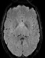
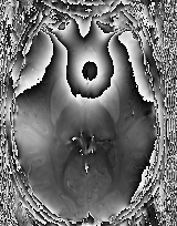
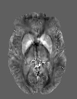
(a)	(b)	(c)

Figure 22: Example for integrative TGV-regularised susceptibility reconstruction from wrapped phase data. (a) Magnitude image (for brain mask extraction). (b) Input phase image $\varphi_{t}$ (single gradient echo, echo time: 27ms, field strength: 3T). (c) Result of the integrative approach (102) (scale from -0.15 to 0.25ppm). All images visualise one slice of the respective 3D image.

8.5 Dynamic MRI reconstruction

As mentioned in Subsection 8.2, data acquisition in MR imaging is relatively slow. This can be compensated by subsampling and variational reconstruction techniques such that in controlled environments, as for instance with brain or knee imaging, a good reconstruction quality can be obtained. The situation is more difficult when imaging parts of the body that are affected, for instance, by breathing motion, or when one aims to image certain dynamics such as with dynamic contrast enhanced MRI or heart imaging. Regarding unwanted motion, there exists a large amount of literature on motion correction techniques (see [195] for a review) which can be separated into prospective and retrospective motion correction and which often rely on additional measurements to estimate and correct for unwanted motion. In contrast to that, dynamic MRI aims to capture certain dynamic processes such as heartbeats, the flow of blood or contrast agent. Here, the approach is often to acquire highly subsampled data, possibly combined with gating techniques, such that motion consistency can be assumed for each single frame of a time series of measurements. The severe lack of data for each frame can then only be mitigated by exploiting temporal correspondences between different measurement times. One way to achieve this is via Tikhonov regularisation of the dynamic inverse problem, which, for instance, amounts to

$$\min_{u\in L^{p}({{]{0,T}[}\times\Omega})}\ \frac{1}{2}\sum_{i=1}^{k}\int_{0}^{T}\|(K_{t}u_{t})_{i}-(f_{t})_{i}\|_{2}^{2}\ \mathrm{d}{t}+\mathcal{R}_{\alpha}(u),$$ (103)

where $p\in[1,\infty]$, $T>0$, $\Omega\subset\mathbf{R}^{d}$ is the image domain, and for almost every $t\in{]{0,T}[}$, $\sigma_{t}$ is a positive, finite Radon measure on $\mathbf{R}^{d}$ that represents the possibly time-dependent Fourier sampling pattern at time $t$, such that $K_{t}:L^{p}({\Omega})\to L^{2}_{\sigma_{t}}({\mathbf{R}^{d},\mathbf{C}})^{k}$ according to (94) models the MR forward operator, and $f_{t}\in L^{2}_{\sigma_{t}}({\mathbf{R}^{d},\mathbf{C}})^{k}$ represents the associated measurement data. Further, $u_{t}$ denotes the evaluation of $u$ at time $t$ which is almost everywhere a function in $L^{p}({\Omega})$. As usual, $\mathcal{R}_{\alpha}$ corresponds to the regularisation functional that can be used to enforce additional regularity constraints. Note that in order to obtain a well-defined formulation for the time-dependent integral, the $\sigma_{t}$ have to vary in a measurable way with $t$ such that the associated $K_{t}$ and the data $f_{t}$ are also measurable in a suitable sense. We refer to [30] for details on the necessary notion and spaces, and an analysis of the above problem in the context of optimal-transport-based regularisation.

In the context of clinical MR applications, temporal Fourier transforms [116], temporal derivatives [2] or combinations thereof [85] have, for instance, been proposed for temporal regularisation. More recently, methods that build on motion-dependent additive decomposition of the dynamic image data into different components have been successful. The work [140] achieves this in a discrete setting via low-rank and sparse decomposition which, for the low-rank component, penalises the singular values of the matrix containing the vectorised frames in each column. In contrast to that, by employing the $\mathop{\rm ICTGV}\nolimits$ functional presented in Subsection 5.3, the work [166] achieves an additive decomposition and adaptive regularisation of the dynamic data via penalising differently weighted spatio-temporal derivatives. There, problem (103) is solved for the choice

$$\mathcal{R}_{\alpha}(u)=\mathop{\rm ICTGV}\nolimits_{\alpha}^{2}(u)=\inf_{w\in\mathop{\rm BV}\nolimits({]{0,T}[}\times\Omega)}\ \mathop{\rm TGV}\nolimits^{2}_{\beta_{1}}(u-w)+\mathop{\rm TGV}\nolimits_{\beta_{2}}^{2}(w),$$

where the $\mathop{\rm TGV}\nolimits_{\beta_{i}}^{2}$ are second-order spatio-temporal TGV functionals that employ different weightings of the components of the spatio-temporal derivatives in such a way that for $\mathop{\rm TGV}\nolimits_{\beta_{1}}^{2}$, changes in time are penalised stronger than changes in space while $\mathop{\rm TGV}\nolimits_{\beta_{2}}^{2}$ acts the other way around. The numerical solution of (103) can again be obtained within the algorithmic framework presented in Section 6 and we refer to [170] for a GPU-accelerated open source implementation and demo scripts.

Figure 23 shows the result of ICTGV-regularised reconstruction of a multi-coil cardiac cine dataset (subsampled with factor $\approx{}11$) and compares to the straightforward sum-of-squares (SOS) reconstruction. Since the SOS reconstruction does not account for temporal correspondences, it is not able to obtain a useful result for a high subsampling factor while the ICTGV-based reconstruction resolves fine details as well as motion dynamics rather well. Figure 24 shows a comparison to the low-rank and sparse (L+S) method of [140] for a second cine dataset with a different view. Here, the parameters for the L+S method where optimised for each experiment separately using the (in practice unknown) ground truth while for ICTGV, the parameters were trained a-priori on a different dataset and fixed afterwards. It can be seen in Figure 24 that both methods perform rather well up the high subsampling factors, where the ICTGV-based is able to recover fine details (highlighted by arrows) that are lost with L+S reconstruction.

Figure 23: Comparison of straightforward sum-of-squares (left) and ICTGV-regularised (right) reconstruction for a dynamic MR dataset with subsampling factor $\approx 11$. Each image shows one frame of the reconstructed image sequence along with the temporal evolution of one horizontal and vertical cross section indicated by the red and blue line, respectively.

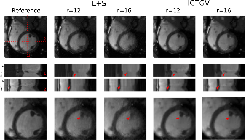
Figure 24: Comparison of L+S- and ICTGV-regularised dynamic MR reconstruction. The first column shows, from top to bottom, a frame of the ground truth image sequence along with the temporal evolution of a vertical and horizontal cross section (indicated by red dotted lines) as well as a close up. Columns 2–3 depict the reconstruction results for L+S regularisation, while columns 4–5 depict the corresponding results for ICTGV regularisation (subsampling factors $r=12$ and $r=16$). The red arrows indicate details that are lost by L+S regularisation but maintained with ICTGV regularisation. Figure taken from [166]. Reprinted by permission from John Wiley and Sons.

8.6 Joint MR-PET reconstruction

We have seen in Subsections 8.2 and 8.5 that image reconstruction from parallel, subsampled MRI data is non-trivial and can greatly be improved with variational regularisation. Beyond MRI and CT, a further medical imaging modality of high clinical relevance is positron emission tomography (PET). As opposed to standard MR imaging, PET imaging is quantitative and builds on reconstructing the spatial distribution of a radioactive tracer that is injected into the patient prior to the measurement. The forward model in PET imaging is the X-ray transform (often combined with resolution modelling) and, since measurements correspond to photon counts, the noise in PET imaging is typically assumed to be Poisson distributed. Reconstructing images from PET measurement data is a non-trivial inverse problem, where difficulties arise, for instance, from high Poisson noise due to limited data acquisition time, dosage restrictions for the radioactive tracer, as well as from limited measurement resolution due to finite detector size and photon acollinearity. As a result, variational reconstruction methods and in particular TV regularisation are employed also in PET imaging to improve reconstruction (see, for instance, [115, 164]).

In a clinical workflow, often both MR and PET images are acquired, which provides two complementary sources of information for diagnoses. This can also be exploited for reconstruction and in particular, for MR-prior-based PET reconstruction methods, which incorporate structural information from the MR image for PET reconstruction, are now well established in theory [104] and in practice [188, 80, 168]. While those methods regard an a-priori reconstructed MR image as fixed, anatomical prior for PET, also joint, synergistic reconstruction is possible and recently became more popular due to the availability of joint MR-PET scanners [121, 81]. An advantage of the latter is that neither of the two images is fixed a-priori and, in principle, a mutual benefit for both modalities due to joint reconstruction is possible. To this aim, the regularisation term needs to incorporate an appropriate coupling of the two modalities, and here we discuss the coupled TGV-based approach of [121] that allows to achieve this.

At first, we consider the forward model for PET imaging, which consists of a convolution followed by an attenuated the X-ray transform and additive corrections. With $\Omega\subset\mathbf{R}^{d}$ the image domain such that $\Omega\subset B_{R}(0)$ for some $R>0$, the X-ray transform can be defined as linear operator $P:L^{p}(\Omega)\rightarrow L^{1}_{\mu}(\Sigma)$, where $p\in[1,\infty]$, $\Sigma\subset\{{(\vartheta,x)}\ \bigl{|}\ {\vartheta\in\mathcal{S}^{d-1},\,x\in\{{\vartheta}\}^{\perp},\,\|x\|<R}\}$, $\Sigma$ is a non-empty and open subset of the tangent bundle to $\mathcal{S}^{d-1}$, via

$$Pu(\vartheta,x)=\int_{\mathbf{R}}u(x+t\vartheta)\ \mathrm{d}{t}.$$

Note that here, $u$ is extended by zero outside $\Omega$ and the measure $\mu$ on $\Sigma$ is induced by the functional

$$\varphi\mapsto\int_{\mathcal{S}}\int_{\{{\vartheta}\}^{\perp}}\varphi(\vartheta,x)\ \mathrm{d}{\mathcal{H}^{d-1}(x)}\ \mathrm{d}{\mathcal{H}^{d-1}(\vartheta)},$$

see [133, Section 3.4] for details. We further denote by $k\in L^{1}(B_{r}(0))$ a convolution kernel with width $r>0$ that models physical limitations in PET imaging, for instance, due to finite detector size and photon acollinearity, see [150]. The PET forward model is then defined as $K_{\mathop{\rm PET}}:L^{p}(\Omega)\rightarrow L^{1}_{\mu}(\Sigma)$

$$u\mapsto K_{\mathop{\rm PET}}u+c,\quad K_{\mathop{\rm PET}}u(\vartheta,x)=a(\vartheta,x)P(u\ast k)(\vartheta,x),$$

where $u\ast k$ denotes the convolution of $u$ and $k$ (using again zero extension), $a\in L^{\infty}_{\mu}(\Sigma)$ with $a>0$ a.e. includes a correction for attenuation and detector sensitivities and $c\in L^{1}_{\mu}(\Sigma)$ with $c\geq 0$ a.e. accounts for additive errors due to random and scattered events. Assuming the noise in PET to be Poisson distributed, we use the Kullback–Leibler divergence as defined in (2) for data fidelity.

For the MR forward model, we use again the parallel MR operator $K_{\mathop{\rm MR}}$ according to (94) in Subsection 8.2 that includes coil sensitivity profiles and a measurement trajectory defined via a finite, positive Radon measure $\sigma$ on $\mathbf{R}^{d}$.

For regularisation, we use an extension of second-order TGV to multi-channel data as discussed in Subsection 5.3, which, as in parallel MR reconstruction, is adapted to complex-valued data. That is, we define $\mathop{\rm TGV}\nolimits_{\alpha}^{2}$ for $u=(u_{1},u_{2})\in L^{1}_{\mathrm{loc}}({\Omega,\mathbf{C}})$ similar to (53), where we use the spectral norm as pointwise dual norm on $\mathop{\rm Sym}\nolimits^{1}(\mathbf{C}^{d})^{2}$ and the Frobenius norm on $\mathop{\rm Sym}\nolimits^{2}(\mathbf{C}^{d})^{2}$. In the primal version of TGV analogous to (35), this results in particular in a pointwise nuclear-norm penalisation of the first-order derivative information $\nabla u-w$ and is motivated by the goal of enforcing pointwise rank one of $\nabla u-w$ in a discretized setting and hence an alignment of level sets.

With these building blocks, a variational model for coupled MR-PET reconstruction can be written as

$$\min_{u=(u_{1},u_{2})\in L^{p}(\Omega,\mathbf{C})^{2}}\ \lambda_{1}\sum_{i=1}^{k}\|(K_{\mathop{\rm MR}}u_{1})_{i}-(f_{1})_{i}\|_{2,\sigma}+\lambda_{2}\mathop{\rm KL}\nolimits(K_{\mathop{\rm PET}}u_{2}+c,f_{2})+\mathop{\rm TGV}\nolimits_{\alpha}^{2}(u)$$

where $(f_{1})_{1},\ldots,(f_{1})_{k}\in L^{2}_{\sigma}({\mathbf{R}^{d},\mathbf{C}})$ and $f_{2}\in L^{1}_{\mu}({\Sigma})$, $f_{2}\geq 0$ almost everywhere is the given measurement data for MR and PET, respectively, and $\lambda_{1},\lambda_{2}>0$ are the weights for the different data terms. Well-posedness for this model follows again by a straightforward adaptation of Proposition 5.17 to the multi-channel setting. Regarding the regularisation parameters $\lambda_{1},\lambda_{2}$, this is a particular case of coupled multi-discrepancy regularisation and we refer to [106] for results on convergence and parameter choice for vanishing noise. A numerical solution can again be obtained with the techniques described in Section 6, where the discrete forward operator $K_{h}$ is vectorised as $K_{h}=\mathop{\rm diag}\nolimits(K_{\mathop{\rm MR},h},K_{\mathop{\rm PET},h})$ with discretized operators $K_{\mathop{\rm MR},h}$ and $K_{\mathop{\rm PET},h}$, and the discrepancy $S_{f_{h}}$ is the component-wise sum of the two discrepancies above in a discrete version.

Numerical results for 3D in-vivo data using this method, together with a comparison to a standard method, can be found in Figure 25 (see also [121] for a more detailed evaluation). As can be seen there, the coupling of the two modalities yield improved reconstruction results in particular for the PET channels, making sharp features and details more visible.

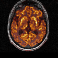
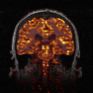
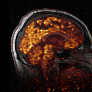
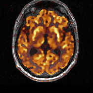
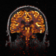
Figure 25: Slices of fused, reconstructed 3D in-vivo MR and PET images from an MPRAGE contrast with 2-fold subsampling and a 10min fluorodeoxyglucose (FDG) PET head scan, respectively (left to right: transversal view, coronal view, sagittal view). Top row: Standard methods (CG sense [147] for MR, expectation maximisation [175] for PET). Bottom row: Nuclear-norm-TGV-based variational reconstruction.

8.7 Radon inversion for multi-channel electron microscopy

Similar to joint MR-PET reconstruction, coupled higher-order regularisation can also be used in multi-channel electron microscopy imaging for improving reconstruction quality. As a particular technique in electron microscopy, scanning transmission electron microscopy (STEM) allows for a three-dimensional imaging of nanomaterials down to atomic resolution and is heavily used in material sciences and nanotechnology, e.g. for quality control and troubleshooting in the production of microchips. Beyond providing pure density images, spectroscopy methods in STEM imaging also allow to image the 3D elemental and chemical make-up of a sample.

Standard techniques for density and spectroscopy imaging in STEM are high-angle annular dark-field (HAADF) imaging and energy-dispersive X-ray spectroscopy (EDXS), respectively. For both imaging methods, measurement data can be acquired simultaneously while raster-scanning the material sample with a focused electron beam. HAADF imaging records the number of electrons scattered to a specific annular range while EDXS allows to record characteristic X-rays for specific elements which are emitted when electrons change their shell position. For each position of the electron beam, both HAADF and EDXS measurements correspond to measuring (approximately) the density of a weighted sum of all elements and single element, respectively, integrated along the line of the electron beam that intersects the sample. Scanning over the entire sample orthogonal to an imaging plane, the acquired signals hence correspond to a slice-wise Radon transform of an overall density image (HAADF) and different elemental maps (EDXS).

Due to physical restrictions in the imaging system, the number of available projections (i.e., measurement angles) as well as the signal-to-noise ratio, in particular for EDXS, is limited and volumetric images obtained with standard image reconstruction methods, such as the simultaneous iterative reconstruction technique (SIRT) [92], suffer from artefacts and noise. As a result, regularised reconstruction is increasingly used also for electron tomography, with total-variation-based methods being a popular example [95]. While TV regularisation works well for piecewise-constant density distributions with sharp interfaces, the presence of gradual changes between different sample regions, e.g., due to diffusion at interfaces, motivates the usage of higher-order regularisation approaches for electron tomography [110], also in a single-channel setting [3]. In a multi-channel setting as discussed here, an additional coupling of different measurement channels is very beneficial in particular for the reconstruction of elemental maps and has been carried out with first-order TV regularisation in [199, 200] and second-order TGV regularisation in [110]. In the following, we discuss the TGV-based approach of [110] in more detail and provide experimental results.

With $\Sigma=\Sigma_{1}\times\Sigma_{2}$, $\Sigma_{1}\subset\mathcal{S}^{1}\times{]{-R,R}[}$ non-empty, open, $\Sigma_{2}\subset{]{-R,R}[}$ non-empty, open, for some $R>0$ and $\mu=(\mathcal{H}^{1}\>\llcornernew\>\mathcal{S}^{1}\times\mathcal{L}^{1})\times\mathcal{L}^{1}$, we define, for $\Omega=B_{R}(0)\times{]{-R,R}[}$ where $B_{R}(0)\subset\mathbf{R}^{2}$ and $p\in[1,\infty]$, the forward operator for electron tomography as $K_{\mathop{\rm TEM}}:L^{p}(\Omega)\rightarrow L^{1}_{\mu}(\Sigma)$ via

$$K_{\mathop{\rm TEM}}u(\vartheta,s,z)=\int_{\{{x\in B_{R}(0)}|{x\cdot\vartheta=s}\}}u(x,z)\ \mathrm{d}{\mathcal{H}^{1}(x)}$$

which corresponds to a slice-wise 2D Radon transform. By continuity of the Radon transform from $L^{1}(B_{R}(0))$ to $L^{1}(\mathcal{S}^{1}\times{]{-R,R}[})$ (see [133, Section 3.4]) there is a $C>0$ such that, for every $u\in L^{p}(B_{R}(0))$ and almost every $z\in{]{-R,R}[}$,

$$\int_{\Sigma_{1}}|K_{\mathop{\rm TEM}}u(\vartheta,s,z)|\ \mathrm{d}{(\mathcal{H}^{1}\times\mathcal{L}^{1})(\vartheta,s)}\leq C\int_{B_{R}(0)}|u(x,z)|\ \mathrm{d}{x}.$$

Integrating over $\Sigma_{2}$, it follows that $K_{\mathop{\rm TEM}}$ is bounded from $L^{p}(\Omega)$ to $L^{1}_{\mu}(\Sigma)$. Now assume $f_{1},\ldots,f_{n}$ to be given, multi-channel measurement data and the forward model for the $i$-th measurement channel to be described with $(K_{\mathop{\rm TEM}})_{i}\in\mathcal{L}(L^{p}(\Omega),L^{1}_{\mu}(\Sigma))$ for $i=1,\ldots,n$. In the example considered below, $f=(f_{\mathop{\rm HAADF}},f_{\mathop{\rm Yb}},f_{\mathop{\rm Al}},f_{\mathop{\rm Si}})$, with $f_{\mathop{\rm HAADF}}$ the HAADF data, and $(f_{\mathop{\rm Yb}},f_{\mathop{\rm Al}},f_{\mathop{\rm Si}})$ the EDXS data for Ytterbium, Aluminum and Silicon, respectively. With $\mathop{\rm TGV}\nolimits_{\alpha}^{2}$ the multi-channel extension of second-order TGV as discussed in Subsection 5.3, using a Frobenius-norm coupling of the different channels, we consider

$$\min_{u\in L^{p}(\Omega)^{n}}\ \sum_{i=1}^{n}\lambda_{i}\mathop{\rm KL}\nolimits(K_{\mathop{\rm TEM}}^{i}u_{i},f_{i})+\mathop{\rm TGV}\nolimits_{\alpha}^{2}(u)$$

for the reconstruction of multi-channel image data, for which well-posedness again results from a multi-channel extension of Proposition 5.17. A numerical solution can be obtained using the framework as described in Section 6 where again the discrete forward operator $K_{h}$ and the discrepancy term $S_{f_{h}}$ are vectorised accordingly, similar as in Subsection 8.6.

Experimental results for this setting and a comparison to other methods can be found in Figure 26, where in particular, separate TGV regularisation of each channel is compared to the Frobenius-norm-based coupling as mentioned above. It can be seen in Figure 26 that using TGV regularisation significantly improves upon the standard SIRT method. Also, a coupling of the different channels is very beneficial in particular for the elemental maps, making material inclusions visible that can hardly be seen with an uncoupled reconstruction. We refer to [110] for a more detailed evaluation (and comparison to TV-based regularisation).

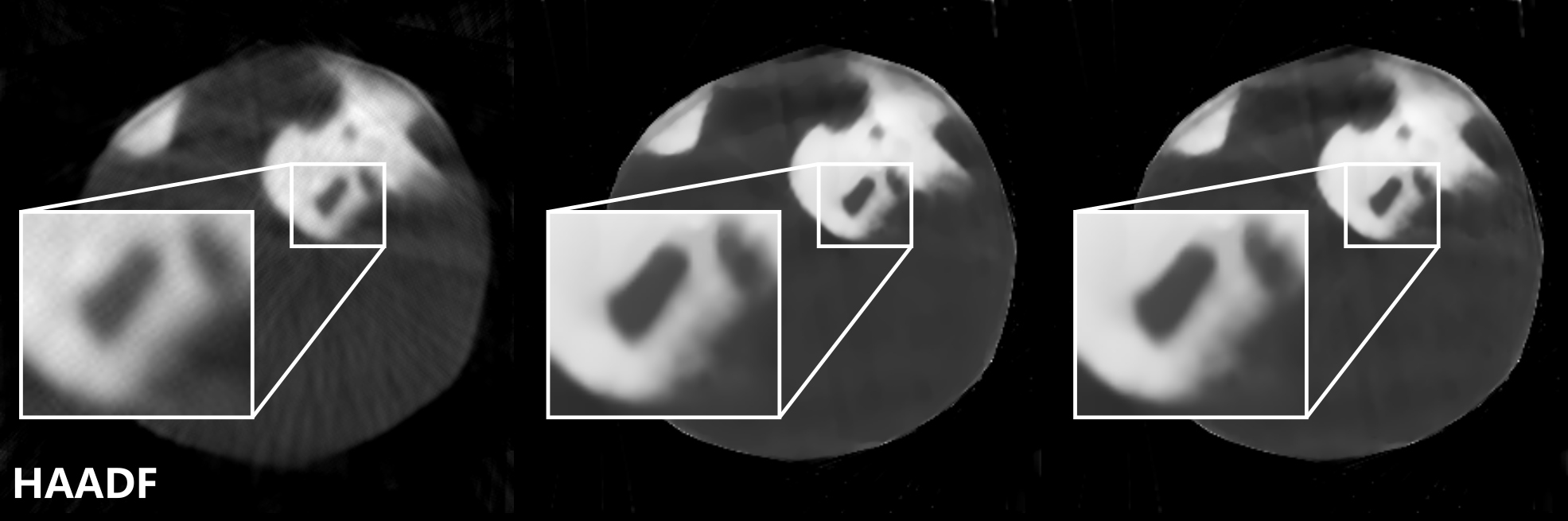
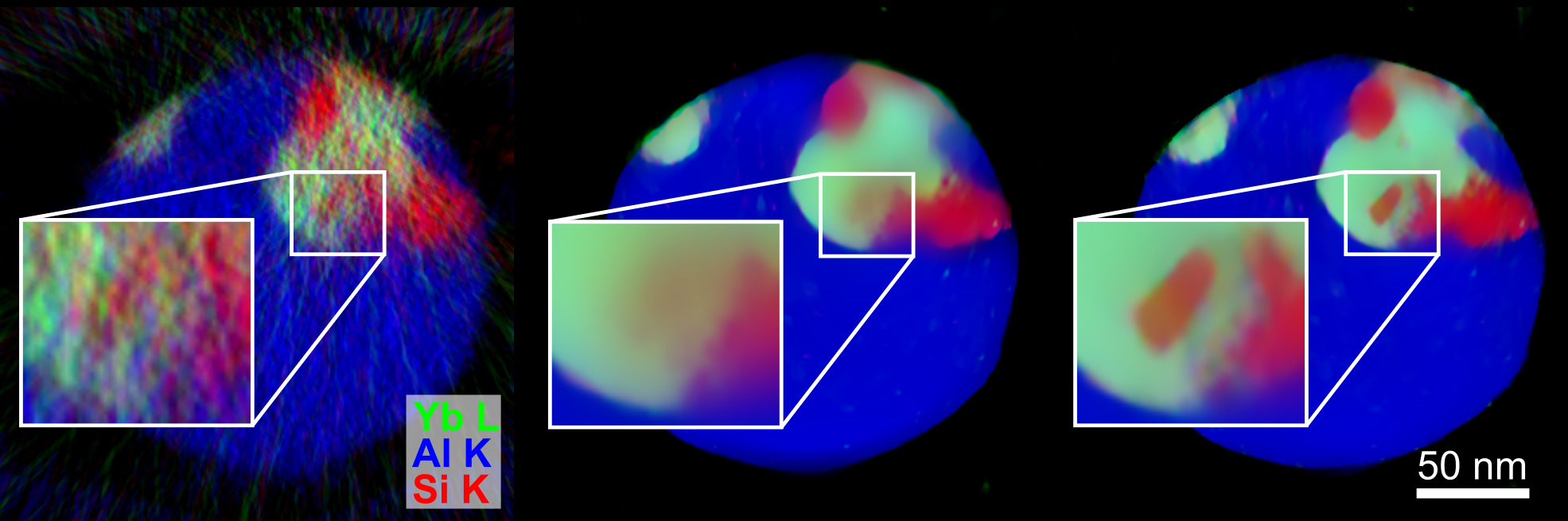
Figure 26: Example of multi-channel electron tomography. The images show density maps (top row) and elemental maps (bottom row) of one slice of a 3D multi-channel electron tomography reconstruction using different reconstruction strategies [110]. Left column: SIRT [92] method. Middle column: Uncoupled TGV-based regularisation. Right column: Coupled TGV-based regularisation. Images taken from [110].

9 Conclusions

The higher-order total variation strategies and application examples discussed in this review show once again that while regularisation makes it possible to solve ill-posed inverse problems in the first place, the actual choice of the regularisation strategy has a tremendous impact on the qualitative properties of the regularised solutions and can be decisive on whether the inverse problem is considered being solved in practice. In the considered context of Tikhonov regularisation, convex regularisation functionals offer a great flexibility in terms of functional-analytic properties and a-priori assumptions on the solutions. With the total variation being an established regulariser sharing desirable properties such as the ability to recover discontinuities, higher-order total variation regularisers offer additional possibilities, mainly the efficient modelling of piecewise smooth regions in which the derivative of some order may jump. We have seen in this paper that a regularisation theory for these functionals can be established and the overall theory is now sufficiently advanced such that the favourable properties of both first- and higher-order TV can be obtained with suitable functionals, for instance by infimal convolution. The underlying concepts are in particular suitable for various generalisations. The total generalised variation, for instance, bases on TV-type penalties for a multiple-order differentiation cascade and thus enables to realise the a-priori assumption of piecewise smoothness with jump discontinuities. Further, due to higher-order derivatives being intrinsically connected to symmetric tensor fields, a generalisation to dedicated regularisation approaches for the latter is immediate. All these approaches and generalisations are indeed beneficial for applications and the solution of concrete inverse problems. This is in particular the case for inverse problems in medical imaging.

Of course, there are still several directions of future research, open questions and topics that have not been covered by this review. For instance, one of the major differences between first-order TV and higher-order approaches is the availability of a co-area formula that can be used to describe the total variation of scalar function in terms of its sublevel-sets. Generalisations to vector-valued functions or higher-order derivatives do either not exist or are not practical from the view of regularisation theory for inverse problems. As the co-area formula allows, for instance, to obtain geometrical properties for TV-regularisation [57, 111], it would be interesting to bridge the gap to higher-order TV approaches such that similar statements can be made. Some recent progress in this direction might be the connection between the solutions of certain linear inverse problems and the extremal points of the sublevel sets of the regulariser [29, 26], since the extremal points of the TV-balls are essentially characteristic functions. However, for higher-order TV and the generalisations discussed in this paper, a characterisation of its extremal points is not known to date. Further, in the context of TV-regularisation, only natural orders of differentiation have been considered in detail so far, with regularisation theory for fractional-order TV just emerging [197, 192, 69]. Indeed, there are many open questions for fractional-order TV regularisation ranging from the properties of the fractional derivative operators and their underlying spaces to optimal selection of the fractional differentiation parameter as well as the construction of efficient numerical algorithms. Finally, with all the possibilities of combining distributional differentiation and Radon-norm-penalisation, which are the essential building blocks of the regularisers discussed in this paper, the question arises whether their structure, parameters and differential operators can also be learned by data-driven optimisation. Some results in this direction can already be found in the literature [49, 70], and we expect that more will follow in the future.

References

Appendix A Additional proofs

Lemma A.1.

With $\Omega^{\prime}\subset\mathbf{R}^{d}$ measurable, in accordance with Equation (2), let the functional $\mathop{\rm KL}\nolimits$ on $L^{1}(\Omega^{\prime})^{2}$ be given as

$$(v,f)\mapsto\mathop{\rm KL}\nolimits(v,f)=\left\{\begin{array}[]{rl}\int_{\Omega^{\prime}}f\Bigl{(}\frac{v}{f}-\log\Bigl{(}\frac{v}{f}\Bigr{)}-1\Bigr{)}\ \mathrm{d}{x}&\mbox{if }f\geq 0,\,v\geq 0\mbox{ a.e.},\\ \infty&\mbox{else,}\end{array}\right.$$

where we set the integrand to $v$ where $f=0$ and to $\infty$ where $v=0$ and $f>0$. Then, $\mathop{\rm KL}\nolimits$ is well-defined, non-negative, convex and lower semi-continuous. In case $f\geq 0$ a.e., it holds that $\mathop{\rm KL}\nolimits(v,f)=0$ if and only if $v=f$. Further, for all $v,f\in L^{1}(\Omega^{\prime})$,

$$\|v-f\|_{1}^{2}\leq\left(\frac{2}{3}\|f\|_{1}+\frac{4}{3}\|v\|_{1}\right)\mathop{\rm KL}\nolimits(v,f),$$ (104)

and in particular,

$$\|v\|_{1}\leq 2\bigl{(}\mathop{\rm KL}\nolimits(v,f)+\|f\|_{1}\bigr{)}\quad\mbox{and}\quad\|f\|_{1}\leq 2\bigl{(}\mathop{\rm KL}\nolimits(v,f)+\|v\|_{1}\bigr{)}$$ (105)

for all $f,v\in L^{1}(\Omega^{\prime})$.

Proof.

At first note that, in case $f,v\geq 0$, $\mathop{\rm KL}\nolimits$ is given by integrating $g:[0,\infty[^{2}\rightarrow[0,\infty]$ with $g(x,y)=x-y-y\log(\frac{x}{y})$ for $x,y\in{[{0,\infty}[}$, where we use the conventions $0\log(\frac{v}{0})=0$ for $v\geq 0$ and $-f\log(\frac{0}{f})=\infty$ for $f>0$. It is easy to see that $g$ is non-negative, convex and lower semi-continuous, hence $\mathop{\rm KL}\nolimits$ is well-defined, non-negative, convex, lower semi-continuous and, in case $f\geq 0$ a.e., $\mathop{\rm KL}\nolimits(v,f)=0$ if and only if $v=f$. Also, a simple computation (see [23]) shows that for all $x,y\in[0,\infty[$,

$$(x-y)^{2}\leq(\frac{2y}{3}+\frac{4x}{3})g(x,y).$$

from which the estimate (104) follows with the Cauchy–Schwarz inequality applied to the square root of the above estimate. Now, for the first estimate in (105), we take $f,v\in L^{1}(\Omega^{\prime})$ and note that in case $\|v\|_{1}\leq\|f\|_{1}$, the estimate holds trivially. In the other case, $v\neq 0$ and we observe that (104) implies

$$\|v\|_{1}^{2}-2\|v\|_{1}\|f\|_{1}\leq\frac{2}{3}\|f\|_{1}\mathop{\rm KL}\nolimits(v,f)+\frac{4}{3}\|v\|_{1}\mathop{\rm KL}\nolimits(v,f)$$

from which the claimed estimate follows from rearranging, dividing by $\|v\|_{1}$ and noting that $\|f\|_{1}/\|v\|_{1}\leq 1$. The second estimate in (105) follows analogously. ∎

Lemma A.2.

For $\{{f^{n}}\}$ and $f$ in $L^{1}(\Omega^{\prime})$, let $\mathop{\rm KL}\nolimits(f,f^{n})\rightarrow 0$. Then, $\|f-f^{n}\|_{1}\rightarrow 0$ and for each sequence $\{{v^{n}}\}$ in $L^{1}({\Omega^{\prime}})$ with $v^{n}\rightharpoonup v$ as $n\to\infty$ for $v\in L^{1}({\Omega^{\prime}})$, it holds that

$$\mathop{\rm KL}\nolimits(v,f)\leq\liminf_{n\to\infty}\ \mathop{\rm KL}\nolimits(v^{n},f^{n}).$$

If, in addition, $f^{n}\leq Cf$ a.e. in $\Omega^{\prime}$ for all $n$ and some $C>0$, then for all $v\in L^{1}(\Omega^{\prime})$, we have

$$\limsup_{n\to\infty}\ \mathop{\rm KL}\nolimits(v,f^{n})\leq\mathop{\rm KL}\nolimits(v,f).$$

Proof.

Assume that $\mathop{\rm KL}\nolimits(f,f^{n})\rightarrow 0$. It follows from the second estimate in (105) that $\{{\mathop{\rm KL}\nolimits(f,f^{n})}\}$ bounded implies $\{{\|f^{n}\|_{1}}\}$ bounded which, using (104), yields that $f^{n}\rightarrow f$ in $L^{1}(\Omega^{\prime})$. The $\liminf$ estimate then follows from lower semi-continuity as in Lemma A.1. Now assume that additionally, $f^{n}\leq Cf$ a.e. in $\Omega^{\prime}$ for all $n$ and some $C>0$. By $L^{1}$-convergence we can take a subsequence $\{{f^{n_{k}}}\}$ such that $f^{n_{k}}\to f$ pointwise a.e., and $\lim_{k\rightarrow\infty}\mathop{\rm KL}\nolimits(v,f^{n_{k}})=\limsup_{n\to\infty}\mathop{\rm KL}\nolimits(v,f^{n})$. As $\mathop{\rm KL}\nolimits(f,f^{n_{k}})\to 0$ as $k\to\infty$, we have $\int_{\Omega^{\prime}}f^{n_{k}}\log(f/f^{n_{k}})\ \mathrm{d}{x}\to 0$. Also, since $f\log(v/f)\in L^{1}({\Omega^{\prime}})$ and $f^{n_{k}}/f$, where we set $f^{n_{k}}/f=0$ where $f=0$, is bounded a.e. uniformly with respect to $k$, we have $\int_{\Omega^{\prime}}(f^{n_{k}}/f)f\log(v/f)\ \mathrm{d}{x}\to\int_{\Omega^{\prime}}f\log(v/f)\ \mathrm{d}{x}$ by virtue of Lebesgue’s theorem. Together, we get

$$\limsup_{n\to\infty}\mathop{\rm KL}\nolimits(v,f^{n}) =\lim_{k\to\infty}\mathop{\rm KL}\nolimits(v,f^{n_{k}})$$

$$=\lim_{k\to\infty}\int_{\Omega^{\prime}}v\ \mathrm{d}{x}-\int_{\Omega^{\prime}}\frac{f^{n_{k}}}{f}f\log\Bigl{(}\frac{v}{f}\Bigr{)}\ \mathrm{d}{x}-\int_{\Omega^{\prime}}f^{n_{k}}\log\Bigl{(}\frac{f}{f^{n_{k}}}\Bigr{)}\ \mathrm{d}{x}-\int_{\Omega^{\prime}}f^{n_{k}}\ \mathrm{d}{x}$$

$$=\int_{\Omega^{\prime}}v-f\log\Bigl{(}\frac{v}{f}\Bigr{)}-f\ \mathrm{d}{x}=\mathop{\rm KL}\nolimits(v,f),$$

which is what we wanted to show. ∎

Lemma A.3.

Let $k\geq 1$, $l\geq 0$ and $u:\Omega\to\mathop{\rm Sym}\nolimits^{l}(\mathbf{R}^{d})$ be $(k+l)$-times continuously differentiable such that $\mathcal{E}^{k}u=0$ in $\Omega$. Then, $\nabla^{k+l}\otimes u=0$ in $\Omega$.

Proof.

The statement is a slight generalisation of [28, Proposition 3.1] and its proof is analogous. We present it for the sake of completeness. Choose $a_{1},\ldots,a_{2l+k}\in\mathbf{R}^{d}$. We show that $(\nabla^{k+l}\otimes u)(x)(a_{1},\ldots,a_{2l+k})=0$ for each $x\in\Omega$. For this purpose, let $L\subset\{{1,\ldots,2l+k}\}$ with ${|{L}|}=l$ and denote, dropping the dependence on $x$, by

$$u_{L}=u(a_{\pi(1)},\ldots,a_{\pi(l)})$$

for some bijective $\pi:\{{1,\ldots,l}\}\to L$, giving a $(k+l)$-times differentiable $u_{L}:\Omega\to\mathbf{R}$. Observe that by symmetry, $u_{L}$ does not depend on the choice of $\pi$ but indeed only on $L$. Likewise, denote by

$$\frac{\partial^{k+l}u_{L}}{\partial a_{\complement L}}=(\nabla^{k+l}\otimes u_{L})(a_{\sigma(1)},\ldots,a_{\sigma(k+l)})$$

for some bijective $\sigma:\{{1,\ldots,k+l}\}\to\complement L$. By symmetry of the derivative, $\frac{\partial^{k+l}u_{L}}{\partial a_{\complement L}}:\Omega\to\mathbf{R}$ only depends on $L$. We also introduce an analogous notation for the symmetrised derivative $\mathcal{E}^{k}$:

$$(\mathcal{E}^{k}u)_{\complement L}=\frac{1}{(k+l)!}\sum_{\begin{array}[]{c}\scriptstyle\sigma:\{{1,\ldots,k+l}\}\to\complement L,\\[-2.79996pt] \scriptstyle\sigma\ {\rm bijective}\end{array}}(\nabla^{k}\otimes u)(a_{\sigma(1)},\ldots,a_{\sigma(k+l)}),$$

and, for some $\pi:\{{1,\ldots,l}\}\to L$ bijective,

$$\frac{\partial^{l}(\mathcal{E}^{k}u)_{\complement L}}{\partial a_{L}}=\frac{1}{(k+l)!}\sum_{\begin{array}[]{c}\scriptstyle\sigma:\{{1,\ldots,k+l}\}\to\complement L,\\[-2.79996pt] \scriptstyle\sigma\ {\rm bijective}\end{array}}(\nabla^{k+l}\otimes u)(a_{\pi(1)},\ldots,a_{\pi(l)},a_{\sigma(1)},\ldots,a_{\sigma(k+l)}).$$

Now, as for $\pi:\{{1,\ldots,l}\}\to L$ bijective, the definitions as well as symmetry yield

$$\begin{array}[]{rl}\displaystyle\frac{\partial^{l}(\mathcal{E}^{k}u)_{\complement L}}{\partial a_{L}}\!\!\!&\displaystyle=\frac{1}{(k+l)!}\sum_{\begin{array}[]{c}\scriptstyle K\subset\complement L,\\[-2.79996pt] \scriptstyle{|{K}|}=k\end{array}}\\[3.99994pt] &\displaystyle\sum_{\begin{array}[]{c}\scriptstyle\sigma:\{{1,\ldots,k+l}\}\to\complement L,\\[-2.79996pt] \scriptstyle\sigma(\{{1,\ldots,k}\})=K,\\[-2.79996pt] \scriptstyle\sigma(\{{k+1,\ldots,k+l}\})=\complement L\setminus K\end{array}}(\nabla^{k+l}\otimes u)(a_{\pi(1)},\ldots,a_{\pi(l)},a_{\sigma(1)},\ldots,a_{\sigma(k)},a_{\sigma(k+1)},\ldots,a_{\sigma(k+l)})\\ &\displaystyle=\frac{k!l!}{(k+l)!}\sum_{\begin{array}[]{c}\scriptstyle K\subset\complement L,\\[-2.79996pt] \scriptstyle{|{K}|}=k\end{array}}\frac{\partial^{k+l}u_{\complement L\setminus K}}{\partial a_{\complement(\complement L\setminus K)}}={{k+l}\choose{l}}^{-1}\sum_{\begin{array}[]{c}\scriptstyle M\subset\{{1,\ldots,2l+k}\},\\[-2.79996pt] \scriptstyle{|{M}|}=l,\ L\cap M=\emptyset\end{array}}\frac{\partial^{k+l}u_{M}}{\partial a_{\complement M}},\end{array}$$

we see that each $\frac{\partial^{l}(\mathcal{E}^{k}u)_{\complement L}}{\partial a_{L}}$ can be written as a linear combination of $\frac{\partial^{k+l}u_{M}}{\partial a_{\complement M}}$. Up to the factor ${{k+l}\choose{l}}^{-1}$, the linear mapping that takes the formal vector $\bigl{(}\frac{\partial^{k+l}u_{M}}{\partial a_{\complement M}}\bigr{)}_{M}$ indexed by all $M\subset\{{1,\ldots,2l+k}\}$, ${|{M}|}=l$ to the formal vector $\bigl{(}\frac{\partial^{l}(\mathcal{E}^{k}u)_{\complement L}}{\partial a_{L}}\bigr{)}_{L}$ indexed by all $L\subset\{{1,\ldots,2l+k}\}$, ${|{L}|}=l$ is corresponding to the multiplication with the adjacency matrix of the Kneser graph $K_{2l+k,l}$, see, for instance, [19] for a definition. The latter is regular, which can, for instance, be seen by looking at its eigenvalues which are known to be

$$\lambda_{m}=(-1)^{m}{{k+l-m}\choose{l-m}},\qquad m=0,\ldots,l,$$

see again [19]. Thus, we can find real numbers $(c_{L})_{L}$ indexed by all $L\subset\{{1,\ldots,2k+l}\}$, ${|{L}|}=l$ and independent from $u$, and $a_{1},\ldots,a_{2l+k}$ such that for $M=\{{k+l+1,\ldots,2l+k}\}$, the identity

$$\frac{\partial^{k+l}u_{M}}{\partial a_{\complement M}}=\sum_{\begin{array}[]{c}\scriptstyle L\subset\{{1,\ldots,2l+k}\},\\[-2.79996pt] \scriptstyle{|{L}|}=l,\ L\cap M=\emptyset\end{array}}c_{L}\frac{\partial^{l}(\mathcal{E}^{k}u)_{\complement L}}{\partial a_{L}}$$

holds. If $\mathcal{E}^{k}u=0$, then the right-hand side is $0$ while the left-hand side corresponds to $\nabla^{k+l}u(a_{1},\ldots,a_{2l+k})$. This completes the proof. ∎

Lemma A.4.

Let $k\geq 1$ and $\Omega\subset\mathbf{R}^{d}$ be a bounded Lipschitz domain. For each $u\in\mathop{\rm BV}\nolimits^{k}(\Omega)$ and $\delta>0$, there exists a $u^{\delta}\in\mathop{\rm BV}\nolimits^{k}(\Omega)\cap C^{\infty}(\Omega)$ such that for $\delta\rightarrow 0$,

$$\|u^{\delta}-u\|_{1}\rightarrow 0\quad\mbox{ and }\quad\|\nabla^{m}u^{\delta}\|_{\mathcal{M}}\rightarrow\|\nabla^{m}u\|_{\mathcal{M}}\quad\mbox{for}\quad m=1,\ldots,k,$$

i.e., $\{{u^{\delta}}\}$ converges strictly in $\mathop{\rm BV}\nolimits^{k}(\Omega)$ to $u$ as $\delta\to 0$.

Proof.

The proof builds on the result [32, Lemma 5.4] and techniques from [7, 84]. Choose a sequence of open sets $\{{\Omega_{n}}\}$ such that $\Omega=\bigcup_{n\in\mathbf{N}}\Omega_{n}$, $\overline{\Omega}_{n}\subset\subset\Omega$ for all $n\in\mathbf{N}$ and any point of $\Omega$ belongs to at most four sets $\Omega_{n}$ (cf. [7, Theorem 3.9] for a construction of such sets). Further, let $\{{\varphi^{n}}\}$ be a partition of unity relative to $\{{\Omega_{n}}\}$, i.e., $\varphi^{n}\in\mathcal{C}_{\mathrm{c}}^{\infty}({\Omega_{n}})$ with $\varphi^{n}\geq 0$ for all $n\in\mathbf{N}$ and $\sum_{n=1}^{\infty}\varphi^{n}=1$ pointwise in $\Omega$. Finally, let $\rho\in\mathcal{C}_{\mathrm{c}}^{\infty}({\mathbf{R}^{d}})$ be a standard mollifier, i.e., $\rho$ is radially symmetric, non-negative and satisfies $\int_{\mathbf{R}^{d}}\rho\ \mathrm{d}{x}=1$. Denote by $\rho_{\epsilon}$ the function given by $\rho_{\epsilon}(x)=\epsilon^{-d}\rho(x/\epsilon)$ for $\epsilon>0$.

As $\rho$ is a mollifier and $\varphi^{n}$ has compact support in $\Omega_{n}$, we can find, for any $n\in\mathbf{N}$, an $\epsilon_{n}>0$ such that $\mathop{\rm supp}\nolimits((v\varphi^{n})\ast\rho_{\epsilon_{n}})\subset\Omega_{n}$ for any $v\in\mathop{\rm BD}\nolimits(\Omega,\mathop{\rm Sym}\nolimits^{l}(\Omega))$, $l\in\mathbf{N}$. Further, as shown in [32, Lemma 5.4], for any $v\in\mathop{\rm BD}\nolimits(\Omega,\mathop{\rm Sym}\nolimits^{l}(\Omega))$ fixed, for any $\delta>0$ we can pick a sequence $\{{\epsilon_{n}^{\delta}}\}$ with each $\epsilon_{n}^{\delta}$ being small enough such that with $v^{\delta}=\sum_{n=1}^{\infty}(v\varphi^{n})\ast\rho_{\epsilon_{n}^{\delta}}$, we have

$$\|v^{\delta}-v\|_{1}\leq\delta\quad\mbox{ and }\quad\|\mathcal{E}v^{\delta}\|_{\mathcal{M}}\leq\|\mathcal{E}v\|_{\mathcal{M}}+\delta.$$

In particular, for $u\in\mathop{\rm BV}\nolimits^{k}(\Omega)$ fixed and $v_{l}=\nabla^{l}u\in\mathop{\rm BD}\nolimits^{k-l}(\Omega,\mathop{\rm Sym}\nolimits^{l}(\mathbf{R}^{d}))$ for $l=0,\ldots,k-1$, we can pick a sequence $\{{\epsilon_{n}^{\delta}}\}$ with each component small enough such that

$$\|v_{l}^{\delta}-v_{l}\|_{1}\leq\delta\quad\mbox{ and }\quad\|\mathcal{E}v_{l}^{\delta}\|_{\mathcal{M}}\leq\|\nabla\otimes v_{l}\|_{\mathcal{M}}+\delta\quad\mbox{for}\quad l=0,\ldots,k-1,$$ (106)

since $\nabla\otimes v_{l}=\mathcal{E}v_{l}$. Further we note that, as additional consequence of the Sobolev–Korn inequality of Theorem 3.18, $v_{l}\in H^{k-1-l,1{}}(\Omega,\mathop{\rm Sym}\nolimits^{l}(\mathbf{R}^{d}))$ and hence by the product rule $\mathcal{E}(v_{l-1}\varphi^{n})=(\mathcal{E}v_{l-1})\varphi^{n}+|\!|\!|(v_{l-1}\otimes\nabla\varphi^{n})$, we get

$$\mathcal{E}v_{l-1}^{\delta}-v_{l}^{\delta}=\sum_{n=1}^{\infty}\mathcal{E}(v_{l-1}\varphi^{n})\ast\rho_{\epsilon^{\delta}_{n}}-(v_{l}\varphi^{n})\ast\rho_{\epsilon^{\delta}_{n}}=\sum_{n=1}^{\infty}|\!|\!|(v_{l-1}\otimes\nabla\varphi^{n})\ast\rho_{\epsilon^{\delta}_{n}}.$$

In addition,

$$\sum_{n=1}^{\infty}|\!|\!|(v_{l-1}\otimes\nabla\varphi^{n})=|\!|\!|\Bigl{(}v_{l-1}\otimes\nabla\Bigl{(}\sum_{n=1}^{\infty}\varphi^{n}\Bigr{)}\Bigr{)}=0.$$

Since each $|\!|\!|(v_{l-1}\otimes\nabla\varphi^{n})\in H^{k-l,1{}}(\Omega,\mathop{\rm Sym}\nolimits^{l}(\mathbf{R}^{d}))$, by adaptation of standard mollification results [84, Theorem 5.2.2] we can further reduce any $\epsilon^{\delta}_{n}$ to be small enough such that for each $m=1,\ldots,k$,

$$\Bigl{\|}{\mathcal{E}^{m-l}\left(|\!|\!|(v_{l-1}\otimes\nabla\varphi^{n})\ast\rho_{\epsilon^{\delta}_{n}}-|\!|\!|(v_{l-1}\otimes\nabla\varphi^{n})\right)}\Bigr{\|}_{1}\leq 2^{-n}\delta\quad\mbox{for}\quad l=1,\ldots,m-1.$$

and consequently,

$$\bigl{\|}{\mathcal{E}^{m-l}\Bigl{(}\mathcal{E}v_{l-1}^{\delta}-v_{l}^{\delta}\Bigr{)}}\bigr{\|}_{1}=\Bigl{\|}{\mathcal{E}^{m-l}\Bigl{(}\sum_{n=1}^{\infty}|\!|\!|(v_{l-1}\otimes\nabla\varphi^{n})\ast\rho_{\epsilon^{\delta}_{n}}-|\!|\!|(v_{l-1}\otimes\nabla\varphi^{n})\Bigr{)}}\Bigr{\|}_{1}\leq\delta.$$

Now, setting $u^{\delta}=v_{0}^{\delta}$, we estimate for $m=1,\ldots,k$, using the second estimate in (106) and that $\mathcal{E}v_{m-1}=\nabla^{m}u$ as well as $\mathcal{E}^{m}u^{\delta}=\nabla^{m}u^{\delta}$,

$$\|\nabla^{m}u^{\delta}\|_{\mathcal{M}} =\Bigl{\|}{\Bigl{(}\sum_{l=1}^{m-1}\mathcal{E}^{m-l}(\mathcal{E}v_{l-1}^{\delta}-v_{l}^{\delta})\Bigr{)}+\mathcal{E}v_{m-1}^{\delta}}\Bigr{\|}_{\mathcal{M}}$$

$$\leq\Bigl{(}\sum_{l=1}^{m-1}\|\mathcal{E}^{m-l}(\mathcal{E}v_{l-1}^{\delta}-v_{l}^{\delta})\|_{1}\Bigr{)}+\|\mathcal{E}v_{m-1}^{\delta}\|_{\mathcal{M}}$$

$$\leq m\delta+\|\nabla^{m}u\|_{\mathcal{M}}.$$

This shows in particular that $u^{\delta}\in\mathop{\rm BV}\nolimits^{k}(\Omega)$ and by construction, $u^{\delta}\in\mathcal{C}^{\infty}({\Omega})$. Taking the limit $\delta\rightarrow 0$ and using the lower semi-continuity of $\mathop{\rm TV}\nolimits^{m}$, we finally obtain

$$\|\nabla^{m}u^{\delta}\|_{\mathcal{M}}\rightarrow\|\nabla^{m}u\|_{\mathcal{M}}$$

for $m=1,\ldots,k$ which, together with the first estimate in (106), implies the assertion. ∎

References

- [1] Adams R A 1975 Sobolev Spaces (Academic Press)
- [2] Adluru G, Awate S P, Tasdizen T, Whitaker R T and DiBella E V 2007 Temporally constrained reconstruction of dynamic cardiac perfusion MRI Magnetic Resonance in Medicine 57 1027–1036
- [3] Al-Aleef A, Alekseev A, MacLaren I and Cockshott P 2015 Electron tomography based on a total generalized variation minimization reconstruction technique 31st Picture Coding Symposium (Cairns, Australia)
- [4] Alberti G, Bouchitté G and Dal Maso G 2003 The calibration method for the Mumford–Shah functional and free-discontinuity problems Calculus of Variations and Partial Differential Equations 16 299–333
- [5] Alter F, Durand S and Froment J 2005 Adapted total variation for artifact free decompression of JPEG images Journal of Mathematical Imaging and Vision 23 199–211
- [6] Amar M, Cicco V D and Fusco N 2008 Lower semicontinuity and relaxation results in BV for integral functionals with BV integrants ESAIM: Control, Optimization and Calculus of Variations 14 456–477
- [7] Ambrosio L, Fusco N and Pallara D 2000 Functions of Bounded Variation and Free Discontinuity Problems (Oxford University Press)
- [8] Attouch H and Brezis H 1986 Duality for the sum of convex functions in general Banach spaces Aspects of Mathematics and its Applications 34 125–133
- [9] Bačák M 2014 Computing medians and means in Hadamard spaces SIAM Journal on Optimization 24 1542–1566
- [10] Bačák M, Bergmann R, Steidl G and Weinmann A 2016 A second order non-smooth variational model for restoring manifold-valued images SIAM Journal on Scientific Computing 38 A567–A597
- [11] Baker S, Scharstein D, Lewis J P, Roth S, Black M J and Szeliski R 2011 A database and evaluation methodology for optical flow International Journal of Computer Vision 92 1–31
- [12] Basser P J and Pierpaoli C 1996 Microstructural and physiological features of tissues elucidated by quantitative-diffusion-tensor MRI Journal of Magnetic Resonance, Series B 111 209–219
- [13] Bauschke H H and Combettes P L 2017 Convex analysis and monotone operator theory in Hilbert spaces CMS Books in Mathematics (Springer International Publishing)
- [14] Bergmann R, Fitschen J H, Persch J and Steidl G 2017 Infimal convolution coupling of first and second order differences on manifold-valued images Scale Space and Variational Methods in Computer Vision ed Lauze F, Dong Y and Dahl A B (Springer International Publishing) pp 447–459 ISBN 978-3-319-58771-4
- [15] Bergmann R, Fitschen J H, Persch J and Steidl G 2018 Priors with coupled first and second order differences for manifold-valued image processing Journal of mathematical imaging and vision 60 1459–1481
- [16] Bergounioux M 2016 Mathematical analysis of a inf-convolution model for image processing Journal of Optimization Theory and Applications 168 1–21
- [17] Bergounioux M and Piffet L 2010 A second-order model for image denoising Set Valued Analysis 18 277–306
- [18] Bernstein M A, King K F and Zhou X J 2004 Handbook of MRI pulse sequences (Elsevier)
- [19] Biggs N 1993 Algebraic Graph Theory (Cambridge Mathematical Library no 67) (Cambridge University Press)
- [20] Bilgic B, Fan A P, Polimeni J R, Cauley S F, Bianciardi M, Adalsteinsson E, Wald L L and Setsompop K 2014 Fast quantitative susceptibility mapping with L1-regularization and automatic parameter selection Magnetic Resonance in Medicine 72 1444–1459
- [21] Block K T, Uecker M and Frahm J 2007 Undersampled radial MRI with multiple coils. Iterative image reconstruction using a total variation constraint. Magnetic Resonance in Medicine 57 1086–1098
- [22] Block T 2008 Advanced Methods for Radial Data Sampling in MRI Ph.D. thesis Georg-August-Universität Göttingen
- [23] Borwein J and Lewis A 1991 Convergence of best entropy estimates SIAM Journal on Optimization 1 191–205
- [24] Borzi A, Ito K and Kunisch K 2003 Optimal control formulation for determining optical flow SIAM Journal on Scientific Computing 24 818–847
- [25] Boyd S, Parikh N, Chu E, Peleato B and Eckstein J 2011 Distributed optimization and statistical learning via the alternating direction method of multipliers Foundations and Trends in Machine Learning 3 1–122
- [26] Boyer C, Chambolle A, Castro Y D, Duval V, De Gournay F and Weiss P 2019 On representer theorems and convex regularization SIAM Journal on Optimization 29 1260–1281
- [27] Bredies K 2014 Recovering piecewise smooth multichannel images by minimization of convex functionals with total generalized variation penalty Efficient Algorithms for Global Optimization Methods in Computer Vision (Lecture Notes in Computer Science vol 8293) ed Bruhn A, Pock T and Tai X C (Springer Berlin Heidelberg) pp 44–77 ISBN 978-3-642-54773-7
- [28] Bredies K 2013 Symmetric tensor fields of bounded deformation Annali di Matematica Pura ed Applicata 192 815–851
- [29] Bredies K and Carioni M 2018 Sparsity of solutions for variational inverse problems with finite-dimensional data arXiv preprint arXiv:1809.05045
- [30] Bredies K and Fanzon S 2019 An optimal transport approach for solving dynamic inverse problems in spaces of measures arXiv preprint arXiv:1901.10162
- [31] Bredies K and Holler M 2012 A total variation-based JPEG decompression model SIAM Journal on Imaging Sciences 5 366–393
- [32] Bredies K and Holler M 2014 Regularization of linear inverse problems with total generalized variation Journal of Inverse and Ill-Posed Problems 22 871–913
- [33] Bredies K and Holler M 2015 A TGV-based framework for variational image decompression, zooming and reconstruction. Part I: Analytics SIAM Journal on Imaging Sciences 8 2814–2850
- [34] Bredies K and Holler M 2015 A TGV-based framework for variational image decompression, zooming and reconstruction. Part II: Numerics SIAM Journal on Imaging Sciences 8 2851–2886
- [35] Bredies K and Holler M 2015 Artifact-free variational MPEG decompression Scale Space and Variational Methods in Computer Vision (Lecture Notes in Computer Science vol 9087) (Springer) pp 216–228
- [36] Bredies K, Holler M, Storath M and Weinmann A 2018 Total generalized variation for manifold-valued data SIAM Journal on Imaging Sciences 11 1785–1848
- [37] Bredies K, Kunisch K and Pock T 2010 Total generalized variation SIAM Journal on Imaging Sciences 3 492–526
- [38] Bredies K, Kunisch K and Valkonen T 2013 Properties of -: The one-dimensional case Journal of Mathematical Analysis and Applications 398 438 – 454
- [39] Bredies K and Lorenz D 2018 Mathematical Image Processing (Springer International Publishing)
- [40] Bredies K and Sun H 2015 Preconditioned Douglas–Rachford splitting methods for convex-concave saddle-point problems SIAM Journal on Numerical Analysis 53 421–444
- [41] Bredies K and Sun H 2015 Preconditioned Douglas-Rachford algorithms for TV- and TGV-regularized variational imaging problems Journal of Mathematical Imaging and Vision 52 317–344
- [42] Bredies K and Sun H 2016 Accelerated Douglas–Rachford methods for the solution of convex-concave saddle-point problems arXiv preprint arXiv:1604.06282
- [43] Bredies K and Sun H 2017 A proximal point analysis of the preconditioned alternating direction method of multipliers Journal of Optimization Theory and Applications 173 878–907
- [44] Bredies K and Vicente D 2018 A perfect reconstruction property for PDE-constrained total-variation minimization with application in Quantitative Susceptibility Mapping ESAIM: COCV
- [45] Briceño-Arias L and Combettes P 2011 A monotone+skew splitting model for composite monotone inclusions in duality SIAM Journal on Optimization 21 1230–1250
- [46] Brown R W, Cheng Y C N, Haacke E M, Thompson M R and Venkatesan R 2014 Magnetic Resonance Imaging: Physical Principles and Sequence Design (John Wiley & Sons)
- [47] Brox T, Bruhn A, Papenberg N and Weickert J 2004 High accuracy optical flow estimation based on a theory for warping Proceedings of the ECCV (Springer) pp 25–36
- [48] Burger M and Osher S 2004 Convergence rates of convex variational regularization Inverse Problems 20 1411–1421
- [49] Calatroni L, Cao C, De Los Reyes J C, Schönlieb C B and Valkonen T 2016 Bilevel approaches for learning of variational imaging models Variational Methods in Imaging and Geometric Control, Radon Series on Computational and Applied Mathematics vol 18 pp 252–290
- [50] Calderón A P and Zygmund A 1952 On the existence of certain singular integrals Acta Mathematica 88 85–139
- [51] Callaghan P T 1991 Principles of Nuclear Magnetic Resonance Microscopy Oxford science publications (Clarendon Press)
- [52] Candès E J, Romberg J and Tao T 2006 Robust uncertainty principles: Exact signal reconstruction from highly incomplete frequency information IEEE Transactions on Information Theory 52 489–509
- [53] Candès E J, Romberg J K and Tao T 2006 Stable signal recovery from incomplete and inaccurate measurements Communications on Pure and Applied Mathematics 59 1207–1223
- [54] Caselles V, Chambolle A and Novaga M 2007 The discontinuity set of solutions of the TV denoising problem and some extensions Multiscale Modelling and Simulation 6 879–894
- [55] Chambolle A 2001 Convex representation for lower semicontinuous envelopes of functionals in Journal of Convex Analysis 8 149–170
- [56] Chambolle A 2004 An algorithm for total variation minimization and applications Journal of Mathematical Imaging and Vision 20 89–97
- [57] Chambolle A, Duval V, Peyré G and Poon C 2016 Geometric properties of solutions to the total variation denoising problem Inverse Problems 33 015002
- [58] Chambolle A and Lions P L 1997 Image recovery via total variation minimization and related problems Numerische Mathematik 76 167–188
- [59] Chambolle A and Pock T 2011 A first-order primal-dual algorithm for convex problems with applications to imaging Journal of Mathematical Imaging and Vision 40 120–145
- [60] Chambolle A and Pock T 2016 On the ergodic convergence rates of a first-order primal–dual algorithm Mathematical Programming 159 253–287
- [61] Chan T F and Esedoḡlu S 2005 Aspects of total variation regularized function approximation SIAM Journal on Applied Mathematics 65 1817–1837
- [62] Chatnuntawech I, McDaniel P, Cauley S F, Gagoski B A, Langkammer C, Martin A, Grant P E, Wald L L, Setsompop K, Adalsteinsson E and Bilgic B 2017 Single-step quantitative susceptibility mapping with variational penalties NMR in Biomedicine 30 e3570
- [63] Chen K and Lorenz D A 2011 Image sequence interpolation using optimal control Journal of Mathematical Imaging and Vision 41 222–238
- [64] Cohen A, Daubechies I and Feauveau J C 1992 Biorthogonal bases of compactly supported wavelets Communications on Pure and Applied Mathematics 45 485–560
- [65] Combettes P L and Pesquet J C 2011 Proximal splitting methods in signal processing Fixed-point algorithms for inverse problems in science and engineering (Springer) pp 185–212
- [66] Cory D G and Garroway A N 1990 Measurement of translational displacement probabilities by NMR: An indicator of compartmentation Magnetic Resonance in Medicine 14 435–444
- [67] Cremers D and Strekalovskiy E 2013 Total cyclic variation and generalizations Journal of Mathematical Imaging and Vision 47 258–277
- [68] Daubechies I, Defrise M and De Mol C 2004 An iterative thresholding algorithm for linear inverse problems with a sparsity constraint Communications on Pure and Applied Mathematics 57 1413–1457
- [69] Davoli E and Liu P 2018 One dimensional fractional order TGV: Gamma-convergence and bilevel training scheme Communications in Mathematical Sciences 16 213–237
- [70] De los Reyes J C, Schönlieb C B and Valkonen T 2016 Bilevel parameter learning for higher-order total variation regularisation models Journal of Mathematical Imaging and Vision 1–25
- [71] Deistung A, Schweser F and Reichenbach J R 2017 Overview of quantitative susceptibility mapping NMR in Biomedicine 30 e3569
- [72] Demengel F 1984 Fonctions à hessien borné Annales de l’institut Fourier 34 155–190
- [73] Deng W and Yin W 2016 On the global and linear convergence of the generalized alternating direction method of multipliers Journal of Scientific Computing 66 889–916
- [74] Deslauriers G, Dubuc S and Lemire D 1999 Une famille d’ondelettes biorthogonales sur l’intervalle obtenue par un schéma d’interpolation itérative Annales des sciences mathématiques du Quéebec 23 37–48
- [75] Di Nezza E, Palatucci G and Valdinoci E 2012 Hitchhiker’s guide to the fractional sobolev spaces Bulletin des Sciences Mathématiques 136 521–573
- [76] Donoho D L 2006 Compressed sensing IEEE T. Inform. Theory 52 1289–1306
- [77] Duarte M F, Davenport M A, Takhar D, Laska J, Sun T, Kelly K and Baraniuk R G 2008 Single-pixel imaging via compressive sampling IEEE Signal Processing Magazine 25 83–91
- [78] Duran J, Möller M, Sbert C and Cremers D 2016 Collaborative total variation: A general framework for vectorial TV models SIAM Journal on Imaging Sciences 9 116–151
- [79] Eckstein J and Bertsekas D P 1992 On the Douglas–Rachford splitting method and the proximal point algorithm for maximal monotone operators Mathematical Programming 55 293–318
- [80] Ehrhardt M, Markiewicz P, Liljeroth M, Barnes A, Kolehmainen V, Duncan J, Pizarro L, Atkinson D, Ourselin S, Hutton B, Thielemans K and Arridge S 2016 PET reconstruction with an anatomical MRI prior using parallel level sets IEEE Transaction on Medical Imaging 35 2189–2199
- [81] Ehrhardt M, Thielemans K, Pizarro L, Atkinson D, Ourselin S, Hutton B and Arridge S 2015 Joint reconstruction of PET-MRI by exploiting structural similarity Inverse Problems 31 015001
- [82] Ekeland I and Témam R 1999 Convex Analysis and Variational Problems (SIAM)
- [83] Engl H W, Hanke M and Neubauer A 2000 Regularization of Inverse Problems (Mathematics and Its Applications vol 375) (Springer)
- [84] Evans L C and Gariepy R F 1992 Measure Theory and Fine Properties of Functions Mathematical Chemistry Series (Taylor & Francis)
- [85] Feng L, Srichai M B, Lim R P, Harrison A, King W, Adluru G, Dibella E V, Sodickson D K, Otazo R and Kim D 2013 Highly accelerated real-time cardiac cine MRI using k–t SPARSE-SENSE Magnetic Resonance in Medicine 70 64–74
- [86] Fessler J and Sutton B 2003 Nonuniform fast Fourier transforms using min-max interpolation IEEE Transactions on Signal Processing 51 560–574
- [87] Flohr T G, McCollough C H, Bruder H, Petersilka M, Gruber K, Süß C, Grasruck M, Stierstorfer K, Krauss B, Raupach R, Primak A N, Küttner A, Achenbach S, Becker C, Kopp A and Ohnesorge B M 2006 First performance evaluation of a dual-source CT (DSCT) system European Radiology 16 1405–1405
- [88] Gabay D 1983 Applications of the method of multipliers to variational inequalities Augmented Lagrangian Methods: Applications to the Numerical Solution of Boundary-Value Problems (Studies in Mathematics and Its Applications vol 15) ed Fortin M and Glowinski R (Elsevier) pp 299–331
- [89] Gao Y and Bredies K 2018 Infimal convolution of oscillation total generalized variation for the recovery of images with structured texture. SIAM Journal on Imaging Sciences 11 2021–2063
- [90] Geiger A, Lenz P and Urtasun R 2012 Are we ready for autonomous driving? The KITTI vision benchmark suite 2012 IEEE Conference on Computer Vision and Pattern Recognition pp 3354–3361
- [91] Gheorghita I P Alina’s eye URL https://www.flickr.com/photos/angel_ina/3201337190/ CC BY 2.0
- [92] Gilbert P 1972 Iterative methods for the three-dimensional reconstruction of an object from projections Journal of Theoretical Biology 36 105–117
- [93] Gilboa G and Osher S 2008 Nonlocal operators with applications to image processing Multiscale Modelling and Simulation 7 1005–1028
- [94] Glowinski R and Marroco A 1975 Sur l’approximation, par éléments finis d’ordre un, et la résolution, par pénalisation-dualité d’une classe de problèmes de Dirichlet non linéaires ESAIM: Mathematical Modelling and Numerical Analysis — Modélisation Mathématique et Analyse Numérique 9 41–76
- [95] Goris B, Van den Broek W, Batenburg K J, Heidari Mezerji H and Bals S 2012 Electron tomography based on a total variation minimization reconstruction technique Ultramicroscopy 113 120–130
- [96] Griswold M A, Jakob P M, Heidemann R M, Nittka M, Jellus V, Wang J, Kiefer B and Haase A 2002 Generalized autocalibrating partially parallel acquisitions (GRAPPA) Magnetic Resonance in Medicine 47 1202–1210
- [97] Grohs P and Sprecher M 2016 Total variation regularization on Riemannian manifolds by iteratively reweighted minimization Information and Inference 5 353–378
- [98] Hackbusch W 2012 Tensor Spaces and Numerical Tensor Calculus (Springer)
- [99] Haffner P, Howard P G, Simard P, Bengio Y, Lecun Y et al. 1998 High quality document image compression with DjVu Journal of Electronic Imaging 7 410–425
- [100] Hammernik K, Klatzer T, Kobler E, Recht M P, Sodickson D K, Pock T and Knoll F 2018 Learning a variational network for reconstruction of accelerated MRI data Magnetic resonance in medicine 79 3055–3071
- [101] He B and Yuan X 2012 Convergence analysis of primal-dual algorithms for a saddle-point problem: From contraction perspective SIAM Journal on Imaging Sciences 5 119–149
- [102] Hinterberger W and Scherzer O 2001 Models for image interpolation based on the optical flow Computing 66 231–247
- [103] Hinterberger W and Scherzer O 2006 Variational methods on the space of functions of bounded Hessian for convexification and denoising Computing 76 109–133
- [104] Hintermüller M, Holler M and Papafitsoros K 2018 A function space framework for structural total variation regularization with applications in inverse problems Inverse Problems 34 064002
- [105] Hofmann B, Kaltenbacher B, Pöschl C and Scherzer O 2007 A convergence rates result for Tikhonov regularization in Banach spaces with non-smooth operators Inverse Problems 23 987–1010
- [106] Holler M, Huber R and Knoll F 2018 Coupled regularization with multiple data discrepancies Inverse Problems 34 084003
- [107] Holler M and Kazimierski K S 2018 Variational decompression of image data from DjVu encoded files IEEE Transactions on Image Processing 27 490–499
- [108] Holler M and Kunisch K 2014 On infimal convolution of TV-type functionals and applications to video and image reconstruction SIAM Journal on Imaging Sciences 7 2258–2300
- [109] Horn B K P and Schunck B G 1981 Determining optical flow Artificial Intelligence 17 185–203
- [110] Huber R, Haberfehlner G, Holler M, Kothleitner G and Bredies K 2019 Total generalized variation regularization for multi-modal electron tomography Nanoscale 11 5617–5632
- [111] Iglesias J A, Mercier G and Scherzer O 2018 A note on convergence of solutions of total variation regularized linear inverse problems Inverse Problems 34 055011
- [112] Ito K and Jin B 2014 Inverse Problems: Tikhonov Theory And Algorithms (Series On Applied Mathematics vol 22) (World Scientific Publishing Company)
- [113] Ivanov V K 1962 On linear problems which are not well-posed Doklady Akademii Nauk SSSR 145 270–272
- [114] Johnson T R C, Krauß B, Sedlmair M, Grasruck M, Bruder H, Morhard D, Fink C, Weckbach S, Lenhard M, Schmidt B, Flohr T, Reiser M F and Becker C R 2007 Material differentiation by dual energy CT: Initial experience European Radiology 17 1510–1517
- [115] Jonsson E, Huang S c and Chan T 1998 Total variation regularization in positron emission tomography CAM report 9848
- [116] Jung H, Sung K, Nayak K S, Kim E Y and Ye J C 2009 k-t FOCUSS: A general compressed sensing framework for high resolution dynamic MRI Magnetic Resonance in Medicine 61 103–116
- [117] Keeling S L and Ring W 2005 Medical image registration and interpolation by optical flow with maximal rigidity Journal of Mathematical Imaging and Vision 23 47–65
- [118] Kheyfets A, Miller W A and Newton G A 2000 Schild’s ladder parallel transport procedure for an arbitrary connection International Journal of Theoretical Physics 39 2891–2898
- [119] Kikuchi N and Oden J 1988 Contact Problems in Elasticity (Society for Industrial and Applied Mathematics)
- [120] Knoll F, Bredies K, Pock T and Stollberger R 2011 Second order total generalized variation (TGV) for MRI Magnetic Resonance in Medicine 65 480–491
- [121] Knoll F, Holler M, Koesters T, Otazo R, Bredies K and Sodickson D K 2017 Joint MR-PET reconstruction using a multi-channel image regularizer IEEE Transactions on Medical Imaging 36 1–16
- [122] Knoll F, Holler M, Koesters T and Sodickson D K 2015 Joint MR-PET reconstruction using vector valued total generalized variation Proceedings of the International Society for Magnetic Resonance in Medicine vol 23 p 3424
- [123] Komodakis N and Pesquet J C 2015 Playing with duality: An overview of recent primal-dual approaches for solving large-scale optimization problems IEEE Signal Processing Magazine 32 31–54
- [124] Kongskov R D and Dong Y 2018 Tomographic reconstruction methods for decomposing directional components Inverse Problems & Imaging 12 1429–1442
- [125] Langkammer C, Bredies K, Poser B A, Barth M, Reishofer G, Fan A P, Bilgic B, Fazekas F, Mainero C and Ropele S 2015 Fast quantitative susceptibility mapping using 3D EPI and total generalized variation Neuroimage 111 622–630
- [126] Lebrun M, Colom M, Buades A and Morel J M 2012 Secrets of image denoising cuisine Acta Numerica 21 475–576
- [127] Lefkimmiatis S, Ward J and Unser M 2013 Hessian Schatten-norm regularization for linear inverse problems IEEE Transactions on Image Processing 22 1873–1888
- [128] Lellmann J, Strekalovskiy E, Koetter S and Cremers D 2013 Total variation regularization for functions with values in a manifold International Conference on Computer Vision (ICCV) pp 2944–2951
- [129] Lions P L and Mercier B 1979 Splitting algorithms for the sum of two nonlinear operators SIAM Journal on Numerical Analysis 16 964–979
- [130] Lu G M, Wu S Y, Yeh B M and Zhang L J 2010 Dual-energy computed tomography in pulmonary embolism The British Journal of Radiology 83 707–718
- [131] Lustig M, Donoho D L and Pauly J M 2007 Sparse MRI: The application of compressed sensing for rapid MR imaging Magnetic Resonance in Medicine 58 1182–1195
- [132] Ma J, März M, Funk S, Schulz-Menger J, Kutyniok G, Schaeffter T and Kolbitsch C 2018 Shearlet-based compressed sensing for fast 3D cardiac MR imaging using iterative reweighting Physics in Medicine & Biology 63 235004
- [133] Markoe A 2006 Analytic Tomography Encyclopedia of Mathematics and its Applications (Cambridge University Press)
- [134] Möllenhoff T, Laude E, Moeller M, Lellmann J and Cremers D 2016 Sublabel-accurate relaxation of nonconvex energies The IEEE Conference on Computer Vision and Pattern Recognition (CVPR)
- [135] Morozov V 1967 Choice of parameter for the solution of functional equations by the regularization method Doklady Akademii Nauk SSSR 175 1225–1228
- [136] Müller T, Rabe C, Rannacher J, Franke U and Mester R 2011 Illumination-robust dense optical flow using census signatures Pattern Recognition ed Mester R and Felsberg M (Springer Berlin Heidelberg) pp 236–245
- [137] Nesterov Y E 2004 Introductory Lectures on Convex Optimization (Applied Optimization vol 87) (Springer)
- [138] Nikolova M 2000 Local strong homogeneity of a regularized estimator SIAM Journal on Applied Mathematics 61 633–658
- [139] Oldham K and Spanier J 1974 The Fractional Calculus (Elsevier Science)
- [140] Otazo R, Candès E and Sodickson D K 2014 Low-rank plus sparse matrix decomposition for accelerated dynamic MRI with separation of background and dynamic components Magnetic Resonance in Medicine 73 1125–1136
- [141] Papafitsoros K and Schönlieb C B 2014 A combined first and second order variational approach for image reconstruction Journal of Mathematical Imaging and Vision 48 308–338
- [142] Pock T and Chambolle A 2011 Diagonal preconditioning for first order primal-dual algorithms in convex optimization 2011 International Conference on Computer Vision (IEEE) pp 1762–1769
- [143] Pock T, Cremers D, Bischof H and Chambolle A 2009 An algorithm for minimizing the Mumford–Shah functional 2009 IEEE 12th International Conference on Computer Vision (IEEE) pp 1133–1140
- [144] Pock T, Cremers D, Bischof H and Chambolle A 2010 Global solutions of variational models with convex regularization SIAM Journal on Imaging Sciences 3 1122–1145
- [145] Podlubny I 1998 Fractional Differential Equations: An Introduction to Fractional Derivatives, Fractional Differential Equations, to Methods of Their Solution and Some of Their Applications (Elsevier Science)
- [146] Poser B, Koopmans P, Witzel T, Wald L and Barth M 2010 Three dimensional echo-planar imaging at 7 Tesla NeuroImage 51 261–266
- [147] Pruessmann K P, Weiger M, Boernert P and Boesiger P 2001 Advances in sensitivity encoding with arbitrary k-space trajectories Magnetic Resonance in Medicine 46 638–651
- [148] Pruessmann K P, Weiger M, Scheidegger M B and Boesiger P 1999 SENSE: Sensitivity encoding for fast MRI Magnetic Resonance in Medicine 42 952–962
- [149] Qin C, Schlemper J, Caballero J, Price A N, Hajnal J V and Rueckert D 2019 Convolutional recurrent neural networks for dynamic MR image reconstruction IEEE transactions on medical imaging 38 280–290
- [150] Rahmim A, Qi J and Sossi V 2013 Resolution modeling in PET imaging: Theory, practice, benefits, and pitfalls Medical physics 40 064301
- [151] Ranftl R, Gehrig S, Pock T and Bischof H 2012 Pushing the limits of stereo using variational stereo estimation 2012 IEEE Intelligent Vehicles Symposium pp 401–407
- [152] Ranftl R 2013 Alternating minimization + Image-driven TGV and census-based data term KITTI Vision Benchmark Suite URL http://www.cvlibs.net/datasets/kitti/eval_stereo_flow_detail.php?benchmark=stereo&error=3&eval=all&result=a7b77e8fddfa90949754d01a1d09b6d8bbabdbb7 CC BY-NC-SA 3.0
- [153] Ranftl R, Bredies K and Pock T 2014 Non-local total generalized variation for optical flow estimation Computer Vision – ECCV 2014 ed Fleet D, Pajdla T, Schiele B and Tuytelaars T (Springer International Publishing) pp 439–454
- [154] Ranftl R, Pock T and Bischof H 2013 Minimizing TGV-based variational models with non-convex data terms Scale Space and Variational Methods in Computer Vision (Springer Berlin Heidelberg) pp 282–293 ISBN 978-3-642-38266-6
- [155] Recht B, Fazel M and Parrilo P A 2010 Guaranteed minimum-rank solutions of linear matrix equations via nuclear norm minimization SIAM review 52 471–501
- [156] Rice Single-Pixel Camera Project 2007 Compressive-sensing camera URL https://web.archive.org/web/20161231160210/http://dsp.rice.edu/cscamera archived web site
- [157] Ring W 2000 Structural properties of solutions to total variation regularization problems ESAIM: Mathematical Modelling and Numerical Analysis 34 799–810
- [158] Robinson S D, Bredies K, Khabipova D, Dymerska B, Marques J P and Schweser F 2017 An illustrated comparison of processing methods for MR phase imaging and QSM: Combining array coil signals and phase unwrapping NMR in Biomedicine 30 e3601
- [159] Rockafellar R T 1997 Convex analysis Princeton Landmarks in Mathematics (Princeton University Press)
- [160] Rockafellar R T 1976 Monotone operators and the proximal point algorithm SIAM journal on control and optimization 14 877–898
- [161] Rudin L I, Osher S and Fatemi E 1992 Nonlinear total variation based noise removal algorithms Physica D: Nonlinear Phenomena 60 259–268
- [162] Rudin W 1987 Real and complex analysis (Tata McGraw-Hill Education)
- [163] Sapiro G and Ringach D L 1996 Anisotropic diffusion of multivalued images with applications to color filtering IEEE transactions on image processing 5 1582–1586
- [164] Sawatzky A, Brune C, Kösters T, Wübbeling F and Burger M 2013 EM-TV methods for inverse problems with Poisson noise Level set and PDE based reconstruction methods in imaging (Springer) pp 71–142
- [165] Schloegl M, Holler M, Bredies K and Stollberger R 2015 A variational approach for coil-sensitivity estimation for undersampled phase-sensitive dynamic MRI reconstruction. Proceedings of the 23th Annual Meeting of ISMRM, Toronto p 3692
- [166] Schloegl M, Holler M, Schwarzl A, Bredies K and Stollberger R 2017 Infimal convolution of total generalized variation functionals for dynamic MRI Magnetic Resonance in Medicine 78 142–155
- [167] Schofield M A and Zhu Y 2003 Fast phase unwrapping algorithm for interferometric applications Optics Letters 28 1194–1196
- [168] Schramm G, Holler M, Rezaei A, Vunckx K, Knoll F, Bredies K, Boada F and Nuyts J 2017 Evaluation of Parallel Level Sets and Bowsher’s Method as Segmentation-Free Anatomical Priors for Time-of-Flight PET Reconstruction IEEE Transaction on Medical Imaging, 37 590 – 603
- [169] Schuster T, Kaltenbacher B, Hofmann B and Kazimierski K S 2012 Regularization Methods in Banach Spaces (Walter de Gruyter)
- [170] Schwarzl A and Schloegl M 2019 Accelerated Variational Dynamic MRI Reconstruction (AVIONIC) [Software] Zenodo
- [171] Schweser F, Deistung A and Reichenbach J R 2016 Foundations of MRI phase imaging and processing for Quantitative Susceptibility Mapping (QSM) Zeitschrift für Medizinische Physik 26 6–34
- [172] Schweser F, Robinson S D, de Rochefort L, Li W and Bredies K 2017 An illustrated comparison of processing methods for phase MRI and QSM: Removal of background field contributions from sources outside the region of interest NMR in Biomedicine 30 e3604
- [173] Setzer S and Steidl G 2008 Variational methods with higher order derivatives in image processing Approximation XII, Nashboro Press, Brentwood 360–386
- [174] Setzer S, Steidl G and Teuber T 2011 Infimal convolution regularizations with discrete -type functionals Communications in Mathematical Sciences 9 797–827
- [175] Shepp L and Vardi Y 1982 Maximum likelihood reconstruction for emission tomography IEEE Transactions on Medical Imaging 1 113–122
- [176] Shmueli K, de Zwart J A, van Gelderen P, Li T Q, Dodd S J and Duyn J H 2009 Magnetic susceptibility mapping of brain tissue in vivo using MRI phase data Magnetic Resonance in Medicine 62 1510–1522
- [177] Showalter R E 1997 Monotone operators in Banach space and nonlinear partial differential equations (Mathematical Surveys and Monographs vol 49) (American Mathematical Society)
- [178] Sodickson D K and Manning W J 1997 Simultaneous acquisition of spatial harmonics (SMASH): Fast imaging with radiofrequency coil arrays Magnetic resonance in medicine 38 591–603
- [179] Stejskal E O and Tanner J E 1965 Spin diffusion measurements: Spin echoes in the presence of a time‐dependent field gradient The Journal of Chemical Physics 42 288–292
- [180] Strecke M and Goldluecke B 2019 Sublabel-accurate convex relaxation with total generalized variation regularization Pattern Recognition ed Brox T, Bruhn A and Fritz M (Springer International Publishing) pp 263–277
- [181] Tikhonov A N, Leonov A S and Yagola A G 1998 Nonlinear Ill-posed Problems (Chapman & Hall)
- [182] Torrey H C 1956 Bloch equations with diffusion terms Physical Review 104(3) 563–565
- [183] Tuch D S 2004 Q-ball imaging Magnetic Resonance in Medicine 52 1358–1372
- [184] Uecker M, Lai P, Murphy M J, Virtue P, Elad M, Pauly J M, Vasanawala S S and Lustig M 2014 ESPIRiT—an eigenvalue approach to autocalibrating parallel MRI: Where SENSE meets GRAPPA Magnetic resonance in medicine 71 990–1001
- [185] Valkonen T, Bredies K and Knoll F 2013 TGV for diffusion tensors: A comparison of fidelity functions Journal of Inverse and Ill-Posed Problems 21 355–377
- [186] Valkonen T, Bredies K and Knoll F 2013 Total generalized variation in diffusion tensor imaging SIAM Journal on Imaging Sciences 6 487–525
- [187] Vogel C, Roth S and Schindler K 2013 An evaluation of data costs for optical flow German Conference on Pattern Recognition (Springer) pp 343–353
- [188] Vunckx K, Atre A, Baete K, Reilhac A, Deroose C, Laere K V and Nuyts J 2012 Evaluation of three MRI-based anatomical priors for quantitative PET brain imaging IEEE Transaction on Medical Imaging 31 599–612
- [189] Walsh D O, Gmitro A F and Marcellin M W 2000 Adaptive reconstruction of phased array mr imagery Magnetic Resonance in Medicine 43 682–690
- [190] Weinmann A, Demaret L and Storath M 2014 Total variation regularization for manifold-valued data SIAM Journal on Imaging Sciences 7 2226–2257
- [191] Werlberger M 2012 Convex Approaches for High Performance Video Processing Phd thesis Graz University of Technology
- [192] Williams B M, Zhang J and Chen K 2016 A new image deconvolution method with fractional regularisation Journal of Algorithms & Computational Technology 10 265–276
- [193] Zabih R and Woodfill J 1994 Non-parametric local transforms for computing visual correspondence Computer Vision — ECCV ’94 ed Eklundh J O (Springer Berlin Heidelberg) pp 151–158
- [194] Zach C, Pock T and Bischof H 2007 A duality based approach for realtime TV- optical flow Pattern Recognition ed Hamprecht F A, Schnörr C and Jähne B (Springer Berlin Heidelberg) pp 214–223
- [195] Zaitsev M, Maclaren J and Herbst M 2015 Motion artifacts in MRI: A complex problem with many partial solutions Journal of Magnetic Resonance Imaging 42 887–901
- [196] Zalinescu C 2002 Convex Analysis in General Vector Spaces (World Scientific Publishing Company)
- [197] Zhang J and Chen K 2015 A total fractional-order variation model for image restoration with nonhomogeneous boundary conditions and its numerical solution SIAM Journal on Imaging Sciences 8 2487–2518
- [198] Zhong S 1997 Image coding with optimal reconstruction International Conference on Image Processing vol 1 pp 161–164
- [199] Zhong Z, Palenstijn W J, Adler J and Batenburg K J 2018 EDS tomographic reconstruction regularized by total nuclear variation joined with HAADF-STEM tomography Ultramicroscopy 191 34–43
- [200] Zhong Z, Palenstijn W J, Viganò N R and Batenburg K J 2018 Numerical methods for low-dose EDS tomography Ultramicroscopy 194 133–142
- [201] Zhu M and Chan T 2008 An efficient primal-dual hybrid gradient algorithm for total variation image restoration CAM Report 08-34 UCLA
- [202] Ziemer W P 2012 Weakly Differentiable Functions: Sobolev Spaces and Functions of Bounded Variation Graduate Texts in Mathematics (Springer New York)