On the potential of BFAST for monitoring burned areas using multi-temporal Landsat-7 images

Abstract

In this letter, we propose a semi-automatic approach to map burned areas and assess burn severity that does not require prior knowledge of the fire date. First, we apply BFAST to NDVI time series and estimate statistically abrupt changes in NDVI trends. These estimated changes are then used as plausible fire dates to calculate dNBR following a typical pre-post fire assessment. In addition to its statistical guarantees, this method depends only on a tuning parameter (the bandwidth of the test statistic for changes). This method was applied to Landsat-7 images taken over La Primavera Flora and Fauna Protection Area, in Jalisco, Mexico, from 2003 to 2016. We evaluated BFAST’s ability to estimate vegetation changes based on time series with significant observation gaps. We discussed burn severity maps associated with massive wildfires (2005 and 2012) and another with smaller dimensions (2008) that might have been excluded from official records. We validated our 2012 burned area map against a high resolution burned area map obtained from RapidEye images; in zones with moderate data quality, the overall accuracy of our map is $92\%$.

I Introduction

Correctly assessing wildfires is an effective means of contributing to the protection of forests and halting biodiversity loss. An indirect and economical way to achieve the latter is to gather satellite-derived products and apply to them a sounding method for mapping burned areas and, subsequently, quantify possible severity or regrowth levels.

When identifying burned areas, three basic aspects should be considered: 1) presence of fuel (in this case, vegetation); 2) abrupt changes in certain spectral indices; and 3) persistence of the abrupt change over time, cf. [1]. Following these principles, several strategies and spectral indices have been used to map burned areas based on Landsat imagery (see [2], [3] [4], [5] and [6] for some related work). In some regions, like the one considered in this letter, Landsat-7 data provides the best spatial (30m) and temporal resolution for vegetation monitoring in general. As a result of the SLC failure of May 2003, however, any analysis using Landsat-7 must factor in an average loss of $22\%$ of the scene’s data.

In this letter, we propose the application of [7]’s BFAST (Breaks For Additive Seasonal Trend) to NDVI and NBR time series of Landsat-7 imagery for burned area mapping, burn severity assessment and long-term monitoring. We also evaluate BFAST’s ability to detect vegetation changes in time series with significant observation gaps. The proposed methodology is applied to data taken over La Primavera Flora and Fauna Protection Area in Jalisco, Mexico between 2003 and 2016. Covering an area of 30,500ha, La Primavera is considered a lung for the metropolitan area of Guadalajara, the third largest city in Mexico. A copy of the code employed for our analysis can be found at the GitHub repository https://github.com/inder-tg/burnSeverity.

II Methodology

BFAST statistically estimates abrupt changes in the trend structure of seasonally-driven time series. More precisely, if $y_{t}$ denotes the value of an NDVI time series at time $t$, BFAST assumes an additive representation for $y_{t}$:

$$~{}y_{t}=T_{t}+S_{t}+\varepsilon_{t},\quad t=1,\ldots,n,$$ (1)

where $T_{t}$ represents the piecewise linear function $T_{t}=\alpha_{j}+\beta_{j}\,t$, $\tau_{j-1}<t\leq\tau_{j}$, with abrupt changes at $\tau_{0}<\tau_{1}<\cdots<\tau_{m}$, $S_{t}$ describes a seasonal component, $\varepsilon_{t}$ denotes white noise with constant variance $\sigma^{2}$, and $n$ is the sample size. Abrupt changes $\tau_{k}$s are estimated using R package bfast, cf. [8]. The user can provide the significance level of the abrupt change test and must set the test statistic bandwidth $h$. For our applications we use a $5\%$ significance level. More details on $h$ can be found in Section VIII-A in the Supplementary Materials.

Let $\widehat{\tau}_{k}$ denote the $k$-th abrupt change estimated by BFAST in an NDVI time series. The dNBR is an appropriate variable to assess wildfire severity in forest vegetation, cf. [9]. Thus, given $\widehat{\tau}_{k}$, its corresponding dNBR is defined as $\mbox{dNBR}(\widehat{\tau}_{k})=\mbox{NBR}_{\widehat{\tau}_{k}-23}-\mbox{NBR}_{\widehat{\tau}_{k}+1}$. Note that the time-point $\widehat{\tau}_{k}-23$ corresponds to almost a year earlier than the estimated breakpoint $\widehat{\tau}_{k}$ whereas $\widehat{\tau}_{k}+1$ is the time-point right after the estimated vegetation change. Using these 2 dates minimizes the differences specifically linked to phenological changes or illumination conditions, cf. [9].

Having calculated $\mbox{dNBR}(\widehat{\tau}_{k})$ we use the values of Table I, adapted from [10], to classify the vegetation change type near $\widehat{\tau}_{k}$. For burned area determination we consider 2 categories: unburned ($\mbox{dNBR}<0.1$) and burned ($\mbox{dNBR}\geq 0.1$). It is customary to summarize the abrupt change estimated by BFAST to the year level, see Section 4.2 of [7]. Thus, we produce annual burned and severity burn maps.

TABLE I: Vegetation change types.

dNBR	Regrowth	Severity
$<-0.25$	High
$-0.25$ to $-0.1$	Low
$-0.1$ to $0.1$		Unburned
$0.1$ to $0.27$		Low
$0.27$ to $0.66$		Moderate
$>0.66$		High

III Data sets

In order to calculate NDVI and NBR we only need spectral bands 3, 4, 5 and 7 from the Landsat-7 images. After proper processing at the L1T level and cloud masking we had 238 of the 322 images expected in the studied period. From our simulations (see Section VIII in the Sup. Mate.), we know that combining linear interpolation and BFAST for estimating one abrupt change in time series with at least $30\%$ missing values yields marginally better results than using spline interpolation. Therefore, we considered linear and spline interpolation as gap filling methods for the NDVI and NBR stack of images. For comparison purposes, in our application we also applied the ArcMap 10.3.1’s low-pass filter with a $3\times 3$ spatial kernel smoother, as well as the algorithm gdal_fillnodata from the GDAL library, cf. [11] to the 238 Landsat-7 images; all remaining gaps were filled in using linear interpolation.

To validate our approach we used a RapidEye burned area polygon for 2012. This polygon’s estimated burned area is based on NDVI, the burned area index proposed by [12], and some empirical thresholds (chosen via visual inspection). This polygon can be seen in Figure 5 along with others provided by governmental agencies.

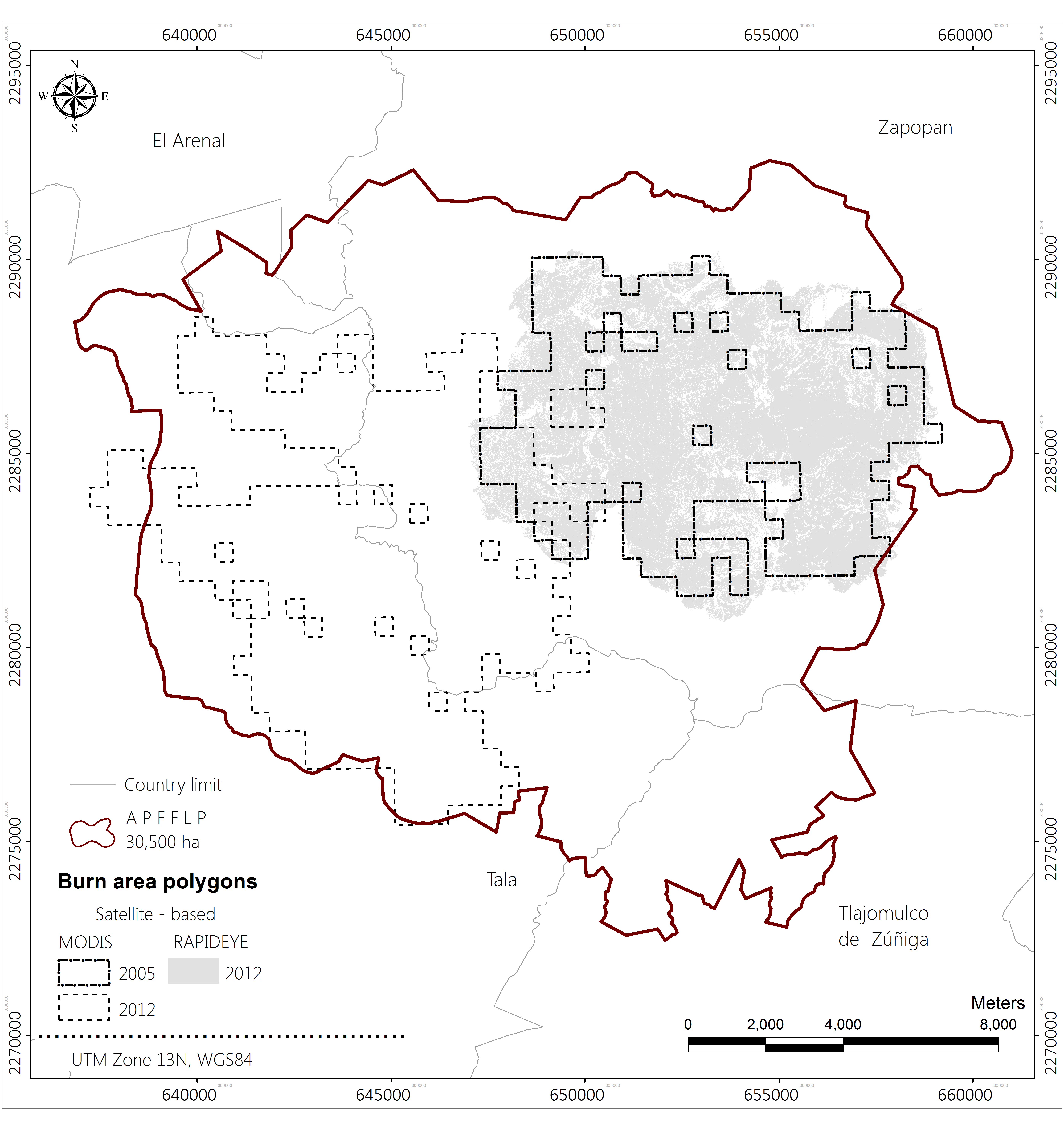
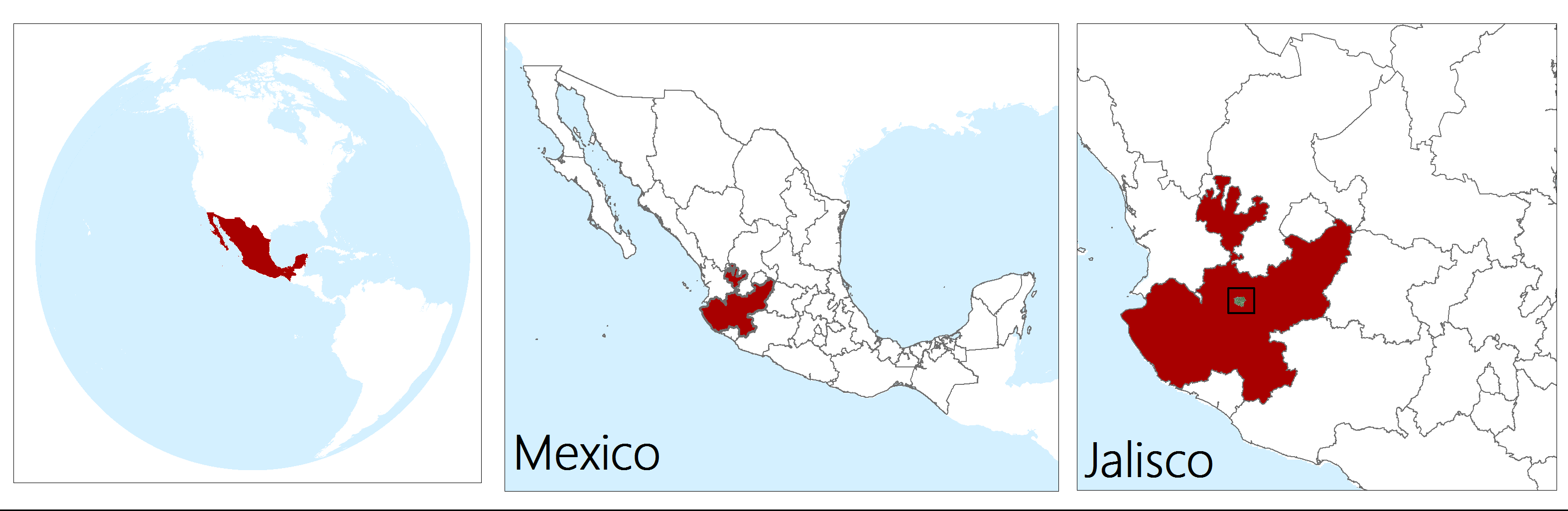
Figure 1: Polygons of estimated burned areas based on MODIS and RapidEye images in La Primavera.

IV Results

Reports of wildfires in La Primavera are available for the period 1998-2012, cf. [13]. Our method detected burned areas between 2005 and 2014, see Table III. Below we comment on the validation and burn severity of some of these burned area maps.

IV-A Accuracy assessment of burned area maps

In this section we assess the overall accuracy of our 2012 burned area map based on Ch. 4 of [14] (see Figure 2). Our aim is to assess overall accuracy as a function of data quality. To this end, we measure the quality of each pixel based on the percentage of missing data in the corresponding NDVI time series (see Fig. 5 in the Sup. Materials). A pixel is said to have poor quality if it has $50$ to $53\%$ missing data. Similarly, a moderate quality pixel is missing $47$ to $49\%$ of data. Based on these definitions, the corresponding overall accuracy was computed (see Table II).

TABLE II: Overall accuracy of 2012 burned area map as a function of data quality and gap filling strategies.

Gap filling method			Overall accuracy ($\%$)
Spatial	Temporal	h	Whole area	Poor data quality	Moderate data quality
	Linear	$0.15$	59.62	70.26	92.36
	Linear	$0.23$	58.93	69.63	90.71
	Spline	$0.15$	61.75	70.52	91.61
	Spline	$0.23$	56.76	67.03	90.39
gdal_fillnodata	Linear	$0.15$	63.31	72.74	92.61
ArcMap filter	Linear	$0.23$	51.05	64.28	90.25

Figure 2: 2012 burned area maps. (A) Lineal interpolation and $h=0.15$. (B) Lineal interpolation and $h=0.23$. (C) Spline interpolation and $h=0.15$. (D) Spline interpolation and $h=0.23$. (E) Interpolated with gdal_fillnodata and $h=0.15$. (F) Interpolated with ArcMap and $h=0.23$.

If all the pixels of the reference RapidEye polygon are considered (see Whole area in Table II), the overall accuracy of our maps is rather low, $51$ to $63\%$. In contrast, if we focus only on areas with poor quality pixels, this overall accuracy improves $11\%$ (on average). This improvement raises even further ($33\%$) when we consider areas with moderate quality pixels. This progressive improvement (from $58.57$ to $91.32\%$ on average) in the overall accuracy suggests that our approach will produce appropriate burned area maps in scenarios where a small amount of data are missing in the original data cubes (NDVI and NBR).

We also evaluate the effect of BFAST’s bandwidth parameter $h$ on our 2005 and 2008 burned area maps. Of the six plots in Figure 2, A and F show a clear spatial discontinuity in the estimated burned area. This apparent discontinuity seems to be resolved when the BFAST’s bandwidth increases ($h=0.23$) and when we use splines as the temporal interpolation method (C-E). Setting these visual features aside, the maps in which $h=0.15$ show the highest overall accuracy irrespective of data quality and gap-filling method. For instance, with Moderate data quality the spatial-temporal gap filling approach (Figure D and gdal_fillnodata row in Table II) seems to produce the same effects on overall accuracy as when only a temporal linear interpolation is applied (Figure A).

IV-B Burned area maps for La Primavera with severity assessment

Burn severity provides a measure of the damage inflicted by fire on an ecosystem, cf. [10]. In order to quantify burn severity, we use Table I.

TABLE III: Estimated burned hectares by year and fraction of burned hectares in La Primavera by level of severity. Here NA stands for not available.

	Total burned area (ha)			Severity Level
				Low			Moderate			High
Year	$h=0.15$	$h=0.23$		$h=0.15$	$h=0.23$		$h=0.15$	$h=0.23$		$h=0.15$	$h=0.23$
2005	3549.24	NA		0.648	NA		0.349	NA		0.003	NA
2006	189.27	729.33		0.888	0.775		0.108	0.224		0.004	0.001
2007	437.58	482.01		0.922	0.933		0.077	0.067		0.001	0.000
2008	1793.34	1156.78		0.695	0.538		0.292	0.431		0.014	0.031
2009	499.86	304.45		0.874	0.951		0.126	0.049		0.000	0.000
2010	402.84	327.18		0.916	0.870		0.083	0.128		0.001	0.003
2011	645.48	620.86		0.908	0.898		0.092	0.102		0.000	0.000
2012	2594.97	2180.61		0.590	0.810		0.398	0.185		0.012	0.005
2013	839.16	1596.44		0.859	0.871		0.139	0.128		0.002	0.001
2014	454.95	NA		0.938	NA		0.062	NA		0.000	NA

Figure 3: Burn severity maps for 2005 and 2008. Linear interpolation. (A) 2005, $h=0.15$. (B) 2008, $h=0.15$. (C) 2008, $h=0.23$. Spline interpolation. (D) 2005, $h=0.15$. (E) 2008, $h=0.15$. (F) 2008, $h=0.23$.

Table III shows that La Primavera’s burn severity is rather low between 2005 and 2014. Because high burn severity has been shown to cause high erosion rates and low vegetation recovery, cf. [15] and [16], we can infer that most of La Primavera’s burned areas suffer from low erosion and profit from a high vegetation regrowth rate.

We now comment on our burn severity maps for the 2005, 2008 and 2012 events. Figure 3-A and D report on the 2005 burned area. In both figures, we require the use of $h=0.15$ as BFAST’s bandwidth parameter (see Section VIII in the Sup. Mate. for further details). In these maps, most of the pixels have been classified as low severity followed by moderate, and to a far less degree, high severity. In 2005, the affected vegetation was primarily native and induced grasslands, followed by shrubs and bushes, and to a less extent, adult woodlands (oak-pine forests). Figure 3-B, C, E and F show the 2008 burned area in the Northeast and Southeast of La Primavera. The majority of this burned area is categorized as low severity, regardless of the bandwidth value. The fraction of burned area categorized as moderate severity is roughly 1.5 times larger for $h=0.23$ than for $h=0.15$. Also, the fraction of burned area categorized under high severity is twice as larger for $h=0.23$ than for $h=0.15$. The vegetation of this area includes oak-pine forests and induced grasslands; to this date there is no official record of the total area damaged (see [13] for more details). Figure 4 shows the 2012 burned area. Independently of the bandwidth value, most of the estimated burned area has been categorized as low severity. Differences seem to emerge for the moderate and high severity categories; the fraction of burned area categorized as moderate severity is twice as larger for $h=0.15$ than for $h=0.23$; a similar result holds for the high severity category. Oak-pine forests and shrubby vegetation dominate this area. According to the state of Jalisco, 10 to 20% of wooded area was lost as a result of this fire, which might have been started in a clandestine landfill.

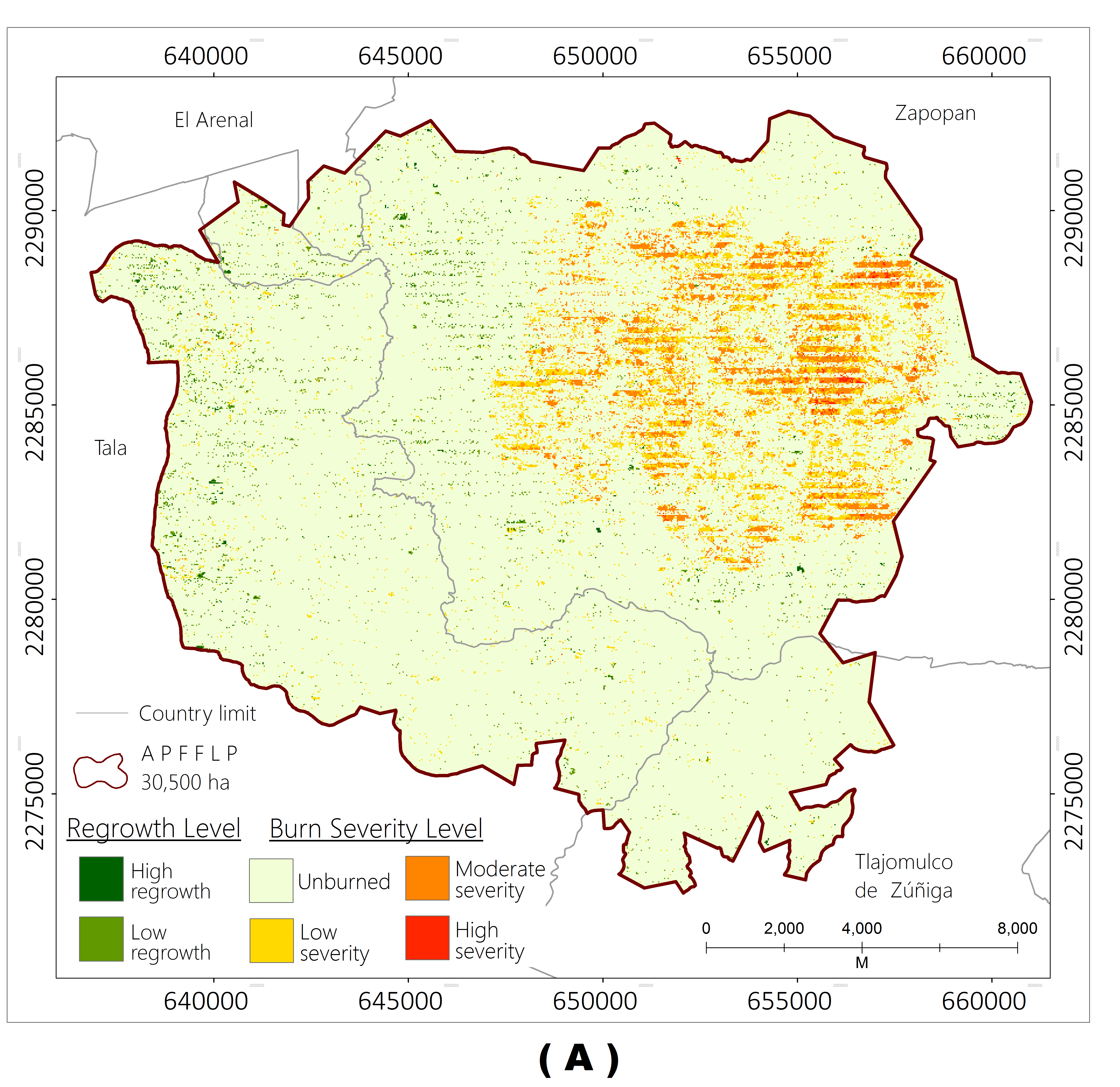
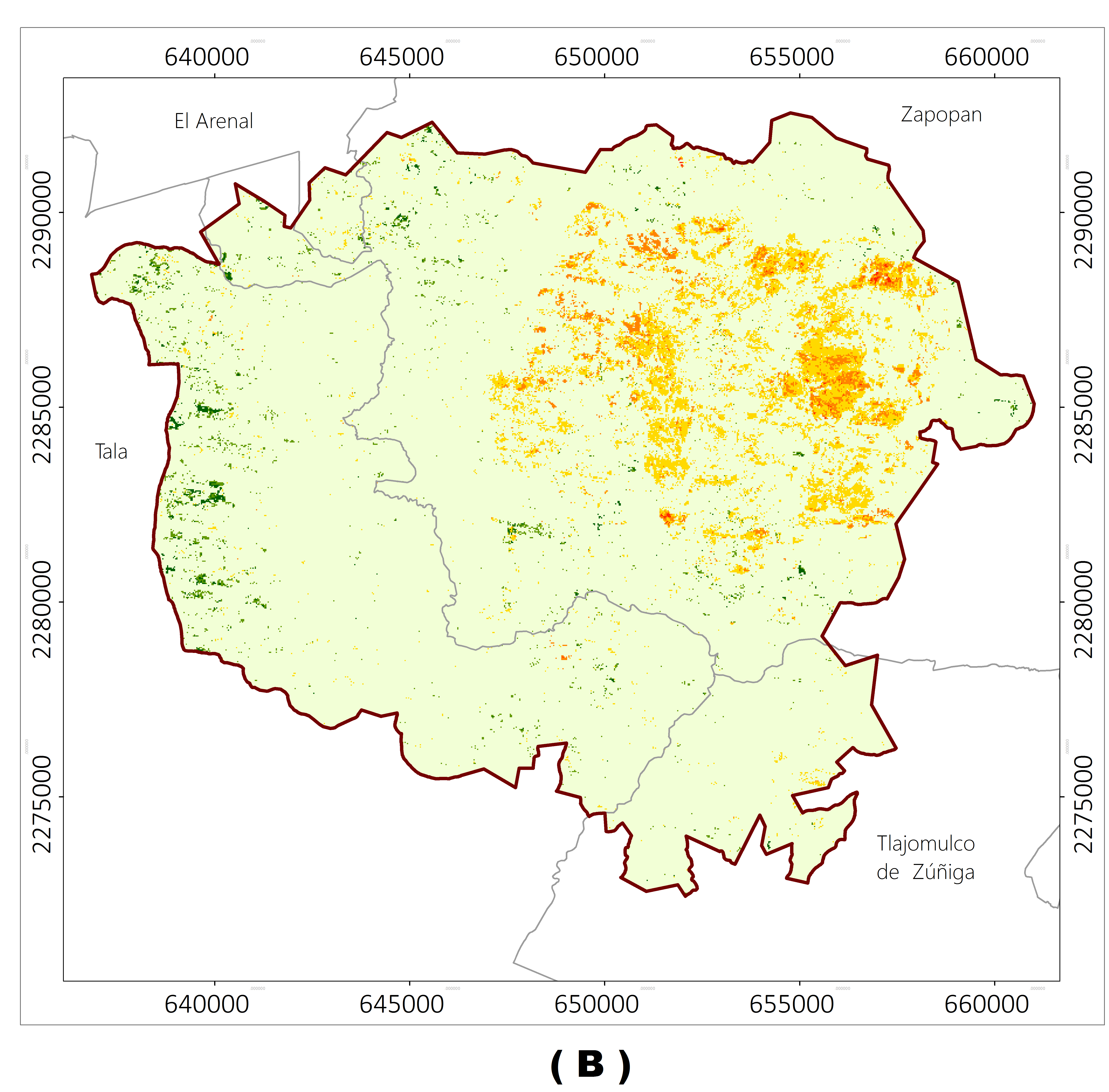
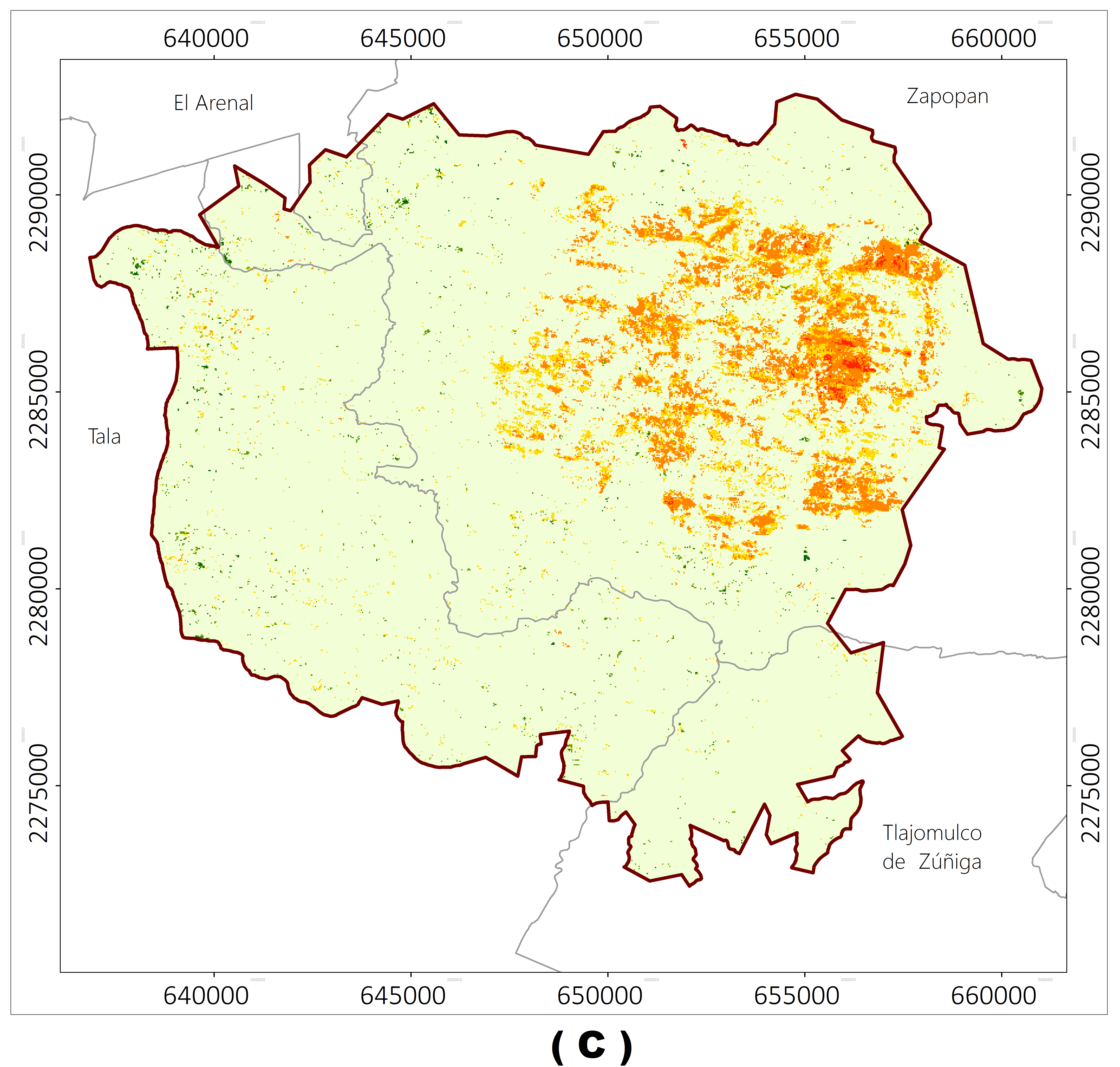
Figure 4: Burn severity maps for 2012. Linear interpolation. (A) $h=0.15$. (B) $h=0.23$. Spline interpolation. (C) 2012, $h=0.15$. (D) 2012, $h=0.23$.

V Conclusion

The proposed method is a semi-automatic approach for burned area mapping and, subsequently, burn severity assessment. Moreover, unlike others, this method provides burned area maps with statistical guarantees. Additionally, using annual burn severity maps, the user can access information on vegetation recovery that may prove useful in many subsequent studies, for instance in fire ecology. The overall accuracy of the annual burned area maps was evaluated in response to the existence of differing amounts of missing data. The overall accuracy of the burned area map that we were able to validate increased from a modest 69% (pixels with poor quality data) to a remarkable 92% (pixels with moderate data quality). This provides evidence that BFAST can be used as an effective and easy-to-apply method for burned area mapping.

VI Acknowledgements

This research was funded by CONACyT’s Convocatoria de Proyectos de Desarrollo Científico para Atender Problemas Nacionales 2016 grant number 2760. The authors would like to thank Lilia de Lourdes Manzo Delgado, Leticia Gómez Mendoza and Stéphane Couturier with the Institute of Geography at UNAM as well as Rainer Ressl with CONABIO for helpful discussions and suggestions. Special thanks to Roberto Martínez with CONABIO for pointing out the function gdal_fillnodata.

Supplementary Materials

VII Supplementary Materials

Figure 5 shows the percentage of missing values in the Landsat-7 NDVI images taken from 2003 to 2016 over La Primavera Flora and Fauna Protection Area in Jalisco, Mexico. In the main manuscript of this letter we used a free-gap version of this data cube to show BFAST’s potential as a tool for mapping burned areas. In this Supplementary Materials we evaluate BFAST’s performance to estimate abrupt changes in synthetic time series sharing the main features, including missing values, of La Primavera’s Landsat-7 NDVI images. We use linear and spline interpolation to fill the gaps of the synthetic time series.

We simulate 16-day NDVI time series from 2003 to 2016 obeying the additive representation given by Eq. $(1)$, see main manuscript. The seasonality ($S_{t}$) and the white noise ($\varepsilon_{t}$) of these synthetic time series are simulated with a harmonic regression model and samples of a normal distribution with zero mean and standard deviation ($\sigma$), respectively. In the next sections we will specify the trend structure, $T_{t}$, as this is different in each study. Each simulation study was repeated 1000 times and we use metrics such as probability coverage and mean squared error (MSE) to assess BFAST’s performance.

Figure 5: Overview of data quality of data cubes for La Primavera: Percentage of missing values in each NDVI pixel.

VIII Simulations

For the amplitude parameter needed in the harmonic model we consider $0.15,0.3$ and $0.45$; for simplicity we use a $0^{\circ}$ phase angle. We consider $\sigma=(0.02,0.05,0.07)$ as these values are in line with the variability level found in La Primavera’s Landsat-7 NDVI time series.

We simulate missing values as follows. From the 322 time-points of any simulated time series ($y_{t}$) we choose randomly and without replacement, $t_{1},\ldots,t_{P}$ say, time-points. Observe that these $P$ time-points are chosen at random, and consequently, there is no order relation among them. Then, the corresponding value in the time series is masked as not available, that is, we set $y_{t_{i}}=\texttt{NA}$, where $i=1,\ldots,P$. In the simulations below we use $P=0,32,64,97,129,161,194$. Approximately, these values corresponds to $0,10,\ldots,50$ and 60% of the total 322 observations.

VIII-A On BFAST’s bandwidth parameter

BFAST utilizes the OLS-MOSUM test to determine statistically the existence of abrupt changes. This test is based on a sequence of partial sums of ordinary least-squares residuals, cf. [17] and [18]; the number of residuals in each sum is fixed, approximately $nh$, but controlled by a bandwidth parameter $0<h<1$; $n$ denotes sample size. Although there are some empirical rules to select the value of $h$, cf. Section 2.2 of [19], our data set does not meet the conditions for these rules to be applied, specially due to the large amount of missing data. Hence, we also include $h$ as a parameter in our simulations; we select $h=0.15,0.23,0.45$. For a time series of 322 observations, $h=0.45$ is equivalent to using a bandwidth of 145 time-points in the aforementioned OLS-MOSUM statistic; this amount of time-points is equivalent to 6 years, approximately, in the Landsat temporal scale.

VIII-B Assessing BFAST’s performance in estimating one abrupt change

In this study the trend has a single abrupt change at the observation 161. Before this observation the trend is constant ($0.7$) and afterwards follows the line $0.3+0.2/161\,t$. More precisely and following Eq. (1), $n=322$, $\alpha_{1}=0.7$, $\alpha_{2}=0.3$, $\beta_{1}=0$, $\beta_{2}=0.2/(161)$, $\tau_{0}=0$, $\tau_{1}=161$, $\tau_{2}=322$ and $m=2$.

As a first goal we are interested in the probability coverage of BFAST to estimate one abrupt change, i.e., the number of times in which an abrupt change is detected divided by the number of simulations. We study probability coverage as a function of the s.d. of the errors of model (1), interpolation method, percentage of missing values, amplitude of the seasonal component and the bandwidth value $h$ utilized by BFAST.

Since a small s.d. benefits both interpolation methods, analysis not included, here we present the results of simulations when we set $\sigma=0.02$ (the smaller value of $\sigma$ under consideration) and allow the bandwidth parameter to vary.

Let us discuss the results of Table IV. Observe that the probability coverage is greater than $0.9$ independently of amplitude, bandwidth and interpolation method even when 20% of observations are missing.

TABLE IV: Probability ($\times 100$) coverage of estimating one abrupt change as a function of the amplitude of the simulated time series, the BFAST’s bandwidth $h$ and the percentage of missing values; here $\sigma=0.02$.

			% of missing values
amplitude	h	methods	0	10	20	30	40	50	60
$0.15$	$0.15$	Linear	99.2	97.9	92.7	79.0	55.9	29.1	10.9
		Spline	99.2	98.2	92.4	83.1	68.9	55.6	41.5
	$0.23$	Linear	99.9	99.7	97.6	92.1	80.5	60.3	39.9
		Spline	99.9	99.3	97.4	93.6	88.3	79.8	68.6
	$0.45$	Linear	100	100	100	100	100	100	100
		Spline	100	100	100	100	100	100	100
$0.3$	$0.15$	Linear	99.8	98.9	95.1	79.7	55.4	23.6	7.9
		Spline	99.8	99.1	95.6	88.7	79.4	67.5	53.3
	$0.23$	Linear	100	99.9	98.4	92.4	78.1	56.1	35.1
		Spline	100	99.8	99.0	96.0	91.9	85.4	74.9
	$0.45$	Linear	100	100	100	100	100	100	100
		Spline	100	100	100	100	100	100	99.9
$0.45$	$0.15$	Linear	100	99.4	95.7	80.6	54.9	22.6	6.9
		Spline	100	99.5	97.6	94.3	87.6	75.9	59.8
	$0.23$	Linear	100	99.9	98.6	92.6	76.7	53.4	31.8
		Spline	100	99.9	99.4	98.3	95.4	89.4	78.8
	$0.45$	Linear	100	100	100	100	100	100	100
		Spline	100	100	100	100	100	100	99.5

The probability coverage is remarkably large when $h=0.45$ independently of amplitude and percentage of missing values. From our next simulation study (Section VIII-C) we infer that utilizing $h=0.45$ in our real data application is equivalent to requiring that the separation between two abrupt changes be of roughly 6 years. Due to this and because our a priori information reports vegetation changes in 2005, 2010, 2012 and 2013, we will not use $h=0.45$ in our application.

For $h=0.15,0.23$ the probability coverage decreases as the percentage of missing values increases. Note that when we use spline-based interpolation the probability coverage is at least $0.68$ in the difficult case of having 60% missing values. In this regard, spline is clearly better than linear interpolation. Observe, however, that this feature only means that is more likely to estimate one abrupt change when we use spline than when we use linear interpolation. This does not tell us much about estimating the correct abrupt change though. Assessing this characteristic is the goal of our next simualation.

TABLE V: Correct estimation probability coverage ($\times 100$) of estimating $\widehat{\tau}_{1}=161$ as a function of the amplitude of the simulated time series, the BFAST’s bandwidth $h$ and the percentage of missing values; here $\sigma=0.02$.

			% of missing values
amplitude	h	methods	0	10	20	30	40	50	60
$0.15$	$0.15$	Linear	100	91.7	80.5	69.7	58.9	53.6	42.2
		Spline	100	91.4	80.2	70.2	60.8	47.8	37.1
	$0.23$	Linear	100	91.4	80.6	70.6	60.2	53.4	45.1
		Spline	100	91.2	80.1	69.9	60.9	49.6	36.3
	$0.45$	Linear	100	91.4	80.5	70.2	60.3	52.6	42.4
		Spline	100	91.3	80.1	70.0	61.7	50.0	37.0
$0.3$	$0.15$	Linear	100	91.3	80.8	69.4	59.0	55.1	43.0
		Spline	100	91.3	80.4	69.2	61.5	49.0	35.3
	$0.23$	Linear	100	91.4	80.7	70.6	61.7	53.8	45.3
		Spline	100	91.3	79.9	69.5	62.0	50.8	35.0
	$0.45$	Linear	100	91.4	80.5	70.9	62.3	54.8	44.8
		Spline	100	91.3	80.0	70.0	61.7	50.8	35.2
$0.45$	$0.15$	Linear	100	91.3	81.1	69.9	58.7	51.8	50.7
		Spline	100	91.1	79.7	68.9	59.7	46.5	28.6
	$0.23$	Linear	100	91.4	81.0	71.1	62.1	56.6	44.7
		Spline	100	91.0	79.2	69.0	59.7	47.2	30.1
	$0.45$	Linear	100	91.4	80.9	71.6	64.0	56.7	45.1
		Spline	100	91.0	79.3	69.5	59.8	47.0	31.0

We also assess BFAST’s correct estimation probability coverage, that is, conditioned on having estimated an abrupt change, we computed the number of times in which the BFAST estimate coincides with the true breakpoint, $\tau_{1}=161$; here we allow amplitude and $h$ to vary but $\sigma=0.02$, see Table V. According to this table BFAST has a perfect correct estimation probability coverage for one abrupt change when the time series is complete, that is, does not have missing values. As the amount of missing values in a time series increases then the correct estimation deteriorates. Moreover, from this table we can infer the following result. Let $0<p<1$ be given. When $100\times p\%$ of observations are missing in a time series and BFAST has estimated one breakpoint, then the probability that this is the true breakpoint is close to $1-p$. Additionally, when 50 to 60% observations are missing from the simulated time series, the correct estimation probability coverage is greater for linear interpolation than for spline interpolation. This characteristic is more evident as the amplitude increases. This is relevant for our application as we deal with a fair amount of time series with roughly 50% missing values.

Finally, BFAST’s accuracy and precision to estimate an abrupt change correctly is reported via the MSE. Figure 6 shows that up to $20\%$ missing values, BFAST’s performance is appropriate independently of the parameter $h$ and interpolation method. From $30\%$ and upwards, the combination of linear interpolation and BFAST outperforms the combination of spline interpolation and BFAST.

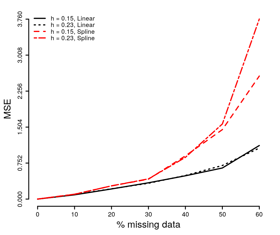
Figure 6: BFAST’s MSE for estimating an abrupt change with $\sigma=0.02$ and amplitude $0.15$

VIII-B1 False negative identification

It is also of interest to assess whether BFAST estimates an abrupt change in the trend of time series with no such change. To this end, we follow Eq. (1) with $T_{t}\equiv 0$. As in the previous simulations, we allow the bandwidth value, amplitude and percentage of missing values to vary. We set $\sigma=0.02$.

TABLE VI: Probability ($\times 100$) of BFAST’s false negative identification as a function of the amplitude of the simulated time series, the BFAST’s bandwidth $h$ and the percentage of missing values; here $\sigma=0.02$.

			% of missing values
amplitude	h	methods	0	10	20	30	40	50	60
$0.15$	$0.15$	Linear	0.1	0.5	3.2	13.6	35.5	66.6	86.6
		Spline	0.1	0.8	3.9	11.4	24.6	39.0	53.9
	$0.23$	Linear	0.3	0.9	3.4	12.1	28.0	52.6	76.3
		Spline	0.3	0.6	3.7	8.4	17.2	30.5	43.2
	$0.45$	Linear	0.0	0.1	0.9	3.3	9.3	20.4	36.4
		Spline	0.0	0.1	1.1	2.1	5.4	8.6	15.0
$0.3$	$0.15$	Linear	0.0	0.2	1.9	11.0	32.0	67.3	88.5
		Spline	0.0	0.5	1.5	6.3	13.5	26.0	39.8
	$0.23$	Linear	0.0	0.4	1.7	10.4	29.0	58.0	80.6
		Spline	0.0	0.7	2.3	4.9	10.3	19.8	31.7
	$0.45$	Linear	0.0	0.4	1.1	3.4	11.0	23.3	37.2
		Spline	0.0	0.2	0.9	1.1	3.2	5.7	10.7
$0.45$	$0.15$	Linear	0.0	0.1	1.1	9.1	28.9	65.2	89.2
		Spline	0.0	0.2	0.7	2.6	7.0	16.9	32.4
	$0.23$	Linear	0.0	0.1	1.2	7.6	28.2	59.9	80.8
		Spline	0.0	0.2	0.7	2.5	5.3	13.4	24.1
	$0.45$	Linear	0.0	0.0	1.0	3.6	11.1	25.1	37.9
		Spline	0.0	0.0	0.4	0.7	2.1	3.2	8.8

The probability that BFAST estimates a non existing abrupt change is nearly zero even when 20% of observations are missing. This feature changes as the amount of missing values reaches 30% (and onwards). In this situation, the false negative probability is far smaller when spline-based fitting is used as an interpolation method than when linear interpolation is employed as a gap filling procedure. These findings are valid regardless bandwidth and amplitude values, see Table VI.

VIII-C Assessing BFAST’s performance in estimating two abrupt changes

Here we are interested in assessing BFAST’s ability to estimate two abrupt changes as a function of the distance between them. We set $\sigma=0.02$, $h=0.15,0.23$, vary the percentage of missing data (from 40 to 60%) and utilize a harmonic regression model to simulate the seasonal component (amplitude $0.15$ and phase angle 0). We focus on the behavior of BFAST when 40 to 60% of observations are missing in the time series based on the results of our previous simulation and because this amount of missing information is relevant for our applications.

In this study the trend function is defined through Eq. (1) with $\alpha_{1}=0.7$, $\alpha_{2}=0.3$, $\alpha_{3}=\alpha_{2}$, $\beta_{1}=0$, $\beta_{2}=0.2/161$, $\beta_{3}=\beta_{2}$, $\tau_{0}=0$, $\tau_{1}=100$, $\tau_{2}=\tau_{1}+\ell$, and $\tau_{3}=322$. Observe that the second abrupt change, $\tau_{2}$, is separated from the first one ($\tau_{1}$) by $\ell$ time-points. In this study we use $\ell=10,20,\ldots,130,140$.

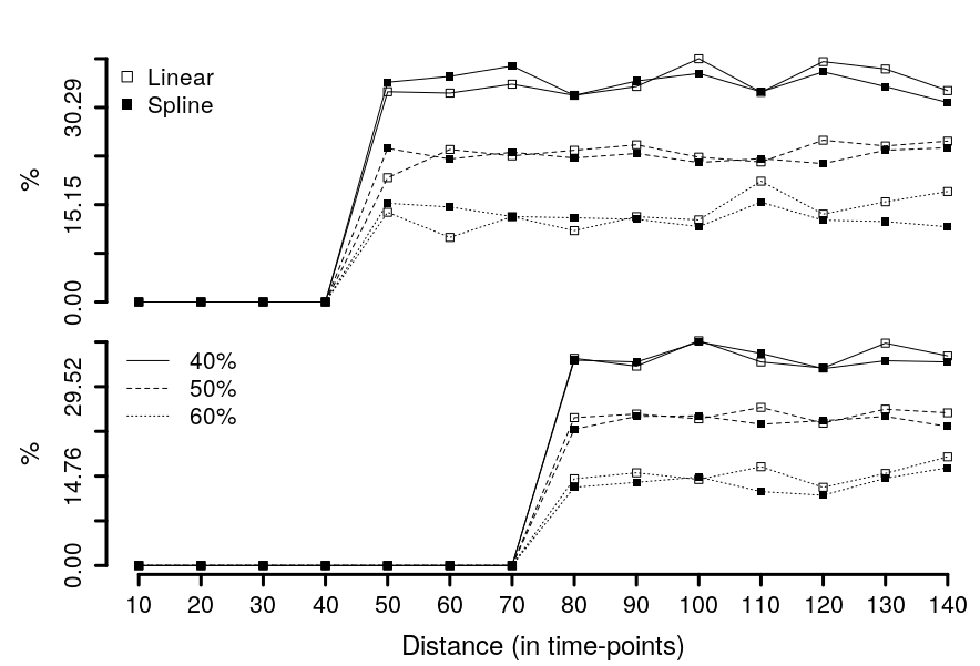
Figure 7: Probability coverage. Bandwidth: $h=0.15$ (top row), $h=0.23$ (bottom row).

We begin by studying BFAST’s probability coverage of estimating correctly the 2 true abrupt changes. That is, we divide the number of times in which BFAST estimates the true abrupt changes $\tau_{1}$ and $\tau_{2}$ by the number of times in which 2 breakpoints are estimated. According to Figure 7, the less percentage of missing data ($40\%$) the greater the BFAST’s probability coverage, regardless of the interpolation method. Also from that figure (top row, $h=0.15$) we infer that in order to obtain a non-zero correct estimation probability is necessary that the abrupt changes are separated by at least 50 time-points (approx. 2 years in Landsat time scale); this is in line with the fact that when $h=0.15$ the OLS-MOSUM statistic uses a bandwidth with roughly 48 time-points. Similarly, (bottom row) when $h=0.23$ (and roughly 75 time-points are used in OLS-MOSUM’s bandwidth) BFAST begins to detect two abrupt changes as soon as they are separated by at least 80 time-points.

Next, we report on BFAST’s underestimation, see Figure 8 for case $h=0.23$. We consider underestimation, i.e. either $\tau_{1}$ or $\tau_{2}$ are estimated correctly, when one (top row), two (middle row) or more than two (bottom row) breakpoints are detected. In the first case, and regardless of the interpolation method, when $40\%$ of data are missing, BFAST underestimates when the separation between $\tau_{1}$ and $\tau_{2}$ is less than 60 time-points. This feature remains true even when 50 and 60% of observations are missing and when linear interpolation is used as gap filling procedure. In the second case (when two abrupt changes are detected), independently of the percentage of missing data and the interpolation method, BFAST’s underestimation reaches a stable level ($45\%$) once the separation is about 80 time-points. Finally, when BFAST has detected more than two abrupt changes, the linear interpolation method shows a less erratic behavior of the underestimation phenomenon throughout different amounts of missing data. Moreover, when 40% of observations are missing and linear interpolation is used, BFAST reaches zero underestimation probability coverage even when the separation between changes is only 10 time-points. Also, BFAST’s underestimation will cease when the breakpoints are separated by 80 time-points.

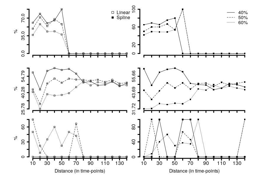
Figure 8: Underestimation. Bandwidth $h=0.23$. Interpolation methods: left column (linear), right column (spline).

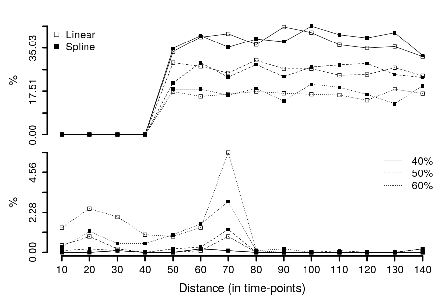
Figure 9: Overestimation. Bandwidth: top row ($h=0.15$), bottom row ($h=0.23$).

From Figure 9 (bottom row) we conclude that when the distance between two breakpoints is at least 80 time-points and $h=0.23$, BFAST does not show overestimation; this feature is independent of the interpolation method and percentage of missing values.

IX Conclusions

The performace of BFAST to estimate abrupt changes deteriorates as the amount of missing values in a time series increases. All in all, BFAST’s performance seems to be less affected by linear than by spline interpolation. For one abrupt change: BFAST’s correct estimation is greater with linear than with spline (even in the difficult case of lacking $50\%$ observations); BFAST’s accuracy and precision is better with linear interpolation (when at least $30\%$ of values are missing); in contrast, the false negative probability is far smaller with spline interpolation. For two abrupt changes linear interpolation shows a marginal better performance than spline interpolation.

As to for BFAST’s bandwidth parameter, the use of $h=0.23$ precludes the detection of burned areas in 2005. Hence, in our application we will also utilize the value $h=0.15$.

References

- [1] E. Chuvieco, L. Giglio, and C. Justice, “Global characterization of fire activity: toward defining fire regimes from Earth observation data,” Global Change Biology, vol. 14, no. 7, pp. 1488–1502, 2008.
- [2] D. Stroppiana, G. Bordogna, M. Boschetti, P. Carrara, L. Boschetti, and P. A. Brivio, “Positive and negative information for assessing and revising scores of burn evidence,” IEEE Geoscience and Remote Sensing Letters, vol. 9, no. 3, pp. 363–367, 2011.
- [3] T. J. Hawbaker, M. K. Vanderhoof, Y.-J. Beal, J. D. Takacs, G. L. Schmidt, J. T. Falgout, B. Williams, N. M. Fairaux, M. K. Caldwell, J. J. Picotte, et al., “Mapping burned areas using dense time-series of landsat data,” Remote Sensing of Environment, vol. 198, pp. 504–522, 2017.
- [4] F. Zhao, C. Huang, and Z. Zhu, “Use of vegetation change tracker and support vector machine to map disturbance types in greater yellowstone ecosystems in a 1984–2010 landsat time series,” IEEE Geoscience and Remote Sensing Letters, vol. 12, no. 8, pp. 1650–1654, 2015.
- [5] D. P. Roy, H. Huang, L. Boschetti, L. Giglio, L. Yan, H. H. Zhang, and Z. Li, “Landsat-8 and Sentinel-2 burned area mapping- A combined sensor multi-temporal change detection approach,” Remote Sensing of Environment, vol. 231, p. 111254, 2019.
- [6] M. Campagnolo, D. Oom, M. Padilla, and J. Pereira, “A patch-based algorithm for global and daily burned area mapping,” Remote Sensing of Environment, vol. 232, p. 111288, 2019.
- [7] J. Verbesselt, R. Hyndman, G. Newnham, and D. Culvenor, “Detecting trend and seasonal changes in satellite image time series,” Remote Sensing of Environment, vol. 114, no. 1, pp. 106–115, 2010.
- [8] J. Verbesselt, A. Zeileis, R. Hyndman, and M. J. Verbesselt, “Package bfast,” 2012.
- [9] S. Escuin, R. Navarro, and P. Fernandez, “Fire severity assessment by using NBR (Normalized Burn Ratio) and NDVI (Normalized Difference Vegetation Index) derived from Landsat TM/ETM images,” International Journal of Remote Sensing, vol. 29, no. 4, pp. 1053–1073, 2008.
- [10] C. H. Key and N. C. Benson, “Landscape Assessment (LA) Sampling and Analysis Methods. USDA Forest Service Gen,” tech. rep., Tech. Rep. RMRS-GTR-164-CD, 2006.
- [11] GDAL, GDAL/OGR Geospatial Data Abstraction software Library. Open Source Geospatial Foundation, 2019.
- [12] M. Martín and E. Chuvieco, “Propuesta de un nuevo índice para cartografía de áreas quemadas: aplicación a imágenes NOAA-AVHRR y Landsat-TM,” Revista de Teledetección, vol. 16, pp. 57–64, 2001.
- [13] F. M. Huerta-Martínez and J. L. Ibarra-Montoya, “Incendios en el bosque La Primavera (Jalisco, México): un acercamiento a sus posibles causas y consecuencias,” CienciaUAT, vol. 9, no. 1, pp. 23–32, 2014.
- [14] R. G. Congalton and K. Green, Assessing the accuracy of remotely sensed data: principles and practices. CRC press, 2 ed., 2009.
- [15] S. Doerr, R. Shakesby, W. Blake, C. Chafer, G. Humphreys, and P. Wallbrink, “Effects of differing wildfire severities on soil wettability and implications for hydrological response,” Journal of Hydrology, vol. 319, no. 1-4, pp. 295–311, 2006.
- [16] J. A. Moody, R. A. Shakesby, P. R. Robichaud, S. H. Cannon, and D. A. Martin, “Current research issues related to post-wildfire runoff and erosion processes,” Earth-Science Reviews, vol. 122, pp. 10–37, 2013.
- [17] C.-S. J. Chu, K. Hornik, and C.-M. Kaun, “MOSUM tests for parameter constancy,” Biometrika, vol. 82, no. 3, pp. 603–617, 1995.
- [18] A. Zeileis, F. Leisch, K. Hornik, and C. Kleiber, “strucchange: An R package for testing for structural change in linear regression models,” Journal of Statistical Software, Articles, vol. 7, no. 2, pp. 1–38, 2002.
- [19] J. Verbesselt, R. Hyndman, A. Zeileis, and D. Culvenor, “Phenological change detection while accounting for abrupt and gradual trends in satellite image time series,” Remote Sensing of Environment, vol. 114, no. 12, pp. 2970–2980, 2010.