Towards Understanding the Spectral Bias of
Deep Learning

Yuan Cao  , Zhiying Fang11footnotemark: 1  , Yue Wu11footnotemark: 1  , Ding-Xuan Zhou , Quanquan Gu Equal contributionDepartment of Computer Science, University of California, Los Angeles, CA 90095, USA; e-mail: yuancao@cs.ucla.eduDepartment of Mathematics, City University of Hong Kong, Kowloon, Hong Kong, China; e-mail: zyfang4-c@my.cityu.edu.hkDepartment of Computer Science, University of California, Los Angeles, CA 90095, USA; e-mail: ywu@cs.ucla.eduDepartment of Mathematics, City University of Hong Kong, Kowloon, Hong Kong, China; e-mail: mazhou@cityu.edu.hkDepartment of Computer Science, University of California, Los Angeles, CA 90095, USA; e-mail: qgu@cs.ucla.edu
Abstract

An intriguing phenomenon observed during training neural networks is the spectral bias, which states that neural networks are biased towards learning less complex functions. The priority of learning functions with low complexity might be at the core of explaining generalization ability of neural network, and certain efforts have been made to provide theoretical explanation for spectral bias. However, there is still no satisfying theoretical result justifying the underlying mechanism of spectral bias. In this paper, we give a comprehensive and rigorous explanation for spectral bias and relate it with the neural tangent kernel function proposed in recent work. We prove that the training process of neural networks can be decomposed along different directions defined by the eigenfunctions of the neural tangent kernel, where each direction has its own convergence rate and the rate is determined by the corresponding eigenvalue. We then provide a case study when the input data is uniformly distributed over the unit sphere, and show that lower degree spherical harmonics are easier to be learned by over-parameterized neural networks. Finally, we provide numerical experiments to demonstrate the correctness of our theory. Our experimental results also show that our theory can tolerate certain model misspecification in terms of the input data distribution.

1 Introduction

Over-parameterized neural networks have achieved great success in many applications such as computer vision (He et al., 2016), natural language processing (Collobert and Weston, 2008) and speech recognition (Hinton et al., 2012). It has been shown that over-parameterized neural networks can fit complicated target function or even randomly labeled data (Zhang et al., 2017) and still exhibit good generalization performance when trained with real labels. Intuitively, this is at odds with the traditional notion of generalization ability such as model complexity. In order to understand neural network training, a line of work (Soudry et al., 2018; Gunasekar et al., 2018b, a) has made efforts in the perspective of “implicit bias”, which states that training algorithms for deep learning implicitly pose an inductive bias onto the training process and lead to a solution with low complexity measured by certain norms in the parameter space of the neural network.

Among many attempts to establish implicit bias, Rahaman et al. (2019) pointed out an intriguing phenomenon called spectral bias, which says that during training, neural networks tend to learn the components of lower complexity faster. Similar observation has also been pointed out in Xu et al. (2019b, a). The concept of spectral bias is appealing because this may intuitively explain why over-parameterized neural networks can achieve a good generalization performance without overfitting. During training, the networks fit the low complexity components first and thus lie in the concept class of low complexity. Arguments like this may lead to rigorous guarantee for generalization.

Great efforts have been made in search of explanations about the spectral bias. Rahaman et al. (2019) evaluated the Fourier spectrum of ReLU networks and empirically showed that the lower frequencies are learned first; also lower frequencies are more robust to random perturbation. Andoni et al. (2014) showed that for a sufficiently wide two-layer network, gradient descent with respect to the second layer can learn any low degree bounded polynomial. Xu (2018) provided Fourier analysis to two-layer networks and showed similar empirical results on one-dimensional functions and real data. Nakkiran et al. (2019) used information theoretical approach to show that networks obtained by stochastic gradient descent can be explained by a linear classifier during early training. These studies provide certain explanations about why neural networks exhibit spectral bias in real tasks. But explanations in the theoretical aspect, if any, are to some extent limited. For example, Fourier analysis is usually done in the one-dimensional setting, and thus lacks generality.

Meanwhile, a recent line of work has taken a new approach to analyze neural networks based on the neural tangent kernel (NTK) (Jacot et al., 2018). In particular, they show that under certain over-parameterization condition, the neural network trained by gradient descent behaves similarly to the kernel regression predictor using the neural tangent kernel. For training a neural network with hidden layer width m𝑚m and sample size n𝑛n, recent optimization results on the training loss in the so-called “neural tangent kernel regime” can be roughly categorized into the following two families: (i) Without any assumption on the target function (the function used to generate the true labels based on the data input), if the network width mpoly(n,λmin1)𝑚poly𝑛superscriptsubscript𝜆1m\geq\mathrm{poly}(n,\lambda_{\min}^{-1}), where λminsubscript𝜆\lambda_{\min} is the smallest eigenvalue of the NTK Gram matrix, then square loss/cross-entropy loss can be optimized to zero (Du et al., 2019b; Allen-Zhu et al., 2019; Du et al., 2019a; Zou et al., 2019; Zou and Gu, 2019); and (ii) If the target function has bounded norm in the NTK-induced reproducing kernel Hilbert space (RKHS), then global convergence can be achieved with milder requirements on m𝑚m. (Arora et al., 2019a, b; Cao and Gu, 2019; Ji and Telgarsky, 2020).

Inspired by these works mentioned above in the neural tangent kernel regime, in this paper we study the spectral bias of over-parameterized two-layer neural networks and its connection to the neural tangent kernel. Note that a basic connection between neural tangent kernel and the spectral bias can be indicated by the observation that neural networks evolve as linear models (Jacot et al., 2018; Lee et al., 2019) in the NTK regime, which suggests that some corresponding results for linear models (Advani and Saxe, 2017) can be applied. However, direct combinations of existing techniques cannot show how many hidden nodes can guarantee the learning of simple/complex components, which is the key problem of interest. Therefore, although such combinations of existing results can provide some mathematical intuition, they are not sufficient to explain the spectral bias for neural networks. To give a thorough characterization of spectral bias, we study the training of mildly over-parameterized neural networks. We show that, given a training data set that is generated based on a target function, a fairly narrow network, although cannot fit the training data well due to its limited width, can still learn certain low-complexity components of the target function in the eigenspace corresponding to large eigenvalues of neural tangent kernel. As the width of the network increases, more high-frequency components of the target function can be learned with a slower convergence rate. As a special case, our result implies that when the input data follows uniform distribution on the unit sphere, polynomials of lower degrees can be learned by a narrower neural network at a faster rate. We also conduct experiments to corroborate the theory we establish.

Our contributions are as follows:

  1. 1.

    We prove a generic theorem for arbitrary data distributions, which states that under certain sample complexity and over-parameterization conditions, the convergence of the training error along different eigendirections of NTK relies on the corresponding eigenvalues. This theorem gives a more precise control on the regression residual than Su and Yang (2019), where the authors focused on the case when the labeling function is close to the subspace spanned by the first few eigenfunctions.

  2. 2.

    We present a characterization of the spectra of the neural tangent kernel that is more general than existing results. In particular, we show that when the input data follow uniform distribution over the unit sphere, the eigenvalues of neural tangent kernel are μk=Ω(max{kd1,dk+1})subscript𝜇𝑘Ωsuperscript𝑘𝑑1superscript𝑑𝑘1\mu_{k}=\Omega(\max\{k^{-d-1},d^{-k+1}\}), k0𝑘0k\geq 0, with corresponding eigenfunctions being the k𝑘k-th order spherical harmonics. Our result is better than the bound Ω(kd1)Ωsuperscript𝑘𝑑1\Omega(k^{-d-1}) derived in Bietti and Mairal (2019) when dkmuch-greater-than𝑑𝑘d\gg k, which is in a more practical setting.

  3. 3.

    We establish a rigorous explanation for the spectral bias based on the aforementioned theoretical results without any specific assumptions on the target function. We show that the error terms from different frequencies are provably controlled by the eigenvalues of the NTK, and the lower-frequency components can be learned with less training examples and narrower networks at a faster convergence rate.

2 Related Work

This paper follows the line of research studying the training of over-parameterized neural networks in the neural tangent kernel regime. As mentioned above, (Du et al., 2019b; Allen-Zhu et al., 2019; Du et al., 2019a; Zou et al., 2019; Zou and Gu, 2019) proved the global convergence of (stochastic) gradient descent regardless of the target function, at the expense of requiring an extremely wide neural network whose width depends on the smallest eigenvalue of the NTK Gram matrix. Another line of work (Arora et al., 2019a; Ghorbani et al., 2019; Arora et al., 2019b; Cao and Gu, 2019; Ji and Telgarsky, 2020) studied the generalization bounds of neural networks trained in the neural tangent kernel regime under various assumptions that essentially require the target function have finite NTK-induced RKHS norm. A side product of these results on generalization is a greatly weakened over-parameterization requirement for global convergence, with the state-of-the-art result requiring a network width only polylogarithmic in the sample size n𝑛n (Ji and Telgarsky, 2020). Su and Yang (2019) studied the network training from a functional approximation perspective, and established a global convergence guarantee when the target function lies in the eigenspace corresponding to the large eigenvalues of the integrating operator Lκf(s):=𝕊dκ(x,s)f(s)𝑑τ(s)assignsubscript𝐿𝜅𝑓𝑠subscriptsuperscript𝕊𝑑𝜅𝑥𝑠𝑓𝑠differential-d𝜏𝑠L_{\kappa}f(s):=\int_{\mathbb{S}^{d}}\kappa(x,s)f(s)d\tau(s), where κ(,)𝜅\kappa(\cdot,\cdot) is the NTK function and τ(s)𝜏𝑠\tau(s) is the input distribution.

A few theoretical results have been established towards understanding the spectra of neural tangent kernels. To name a few, Bach (2017) studied two-layer ReLU networks by relating it to kernel methods, and proposed a harmonic decomposition for the functions in the reproducing kernel Hilbert space which we utilize in our proof. Based on the technique in Bach (2017), Bietti and Mairal (2019) studied the eigenvalue decay of integrating operator defined by the neural tangent kernel on unit sphere by using spherical harmonics. Vempala and Wilmes (2019) calculated the eigenvalues of neural tangent kernel corresponding to two-layer neural networks with sigmoid activation function. Basri et al. (2019) established similar results as Bietti and Mairal (2019), but considered the case of training the first layer parameters of a two-layer networks with bias terms. Yang and Salman (2019) studied the the eigenvalues of integral operator with respect to the NTK on Boolean cube by Fourier analysis. Very recently, Chen and Xu (2020) studied the connection between NTK and Laplacian kernels. Bordelon et al. (2020) gave a spectral analysis on the generalization error of NTK-based kernel ridge regression. Basri et al. (2020) studied the convergence of full training residual with a focus on one-dimensional, non-uniformly distributed data.

A series of papers (Gunasekar et al., 2017; Soudry et al., 2018; Gunasekar et al., 2018a, b; Nacson et al., 2018; Li et al., 2018; Jacot et al., 2020) studied implicit bias problem, aiming to figure out when there are multiple optimal solutions of a training objective function, what kind of nice properties the optimal found by a certain training algorithm would have. Implicit bias results of gradient descent, stochastic gradient descent, or mirror descent for various problem settings including matrix factorization, logistic regression, deep linear networks as well as homogeneous models. The major difference between these results and our work is that implicit bias results usually focus on the parameter space, while we study the functions a neural network prefer to learn in the function space.

3 Preliminaries

In this section we introduce the basic problem setup including the neural network structure and the training algorithm, as well as some background on the neural tangent kernel proposed recently in Jacot et al. (2018) and the corresponding integral operator.

3.1 Notation

We use lower case, lower case bold face, and upper case bold face letters to denote scalars, vectors and matrices respectively. For a vector 𝐯=(v1,,vd)Td𝐯superscriptsubscript𝑣1subscript𝑣𝑑𝑇superscript𝑑\mathbf{v}=(v_{1},\ldots,v_{d})^{T}\in\mathbb{R}^{d} and a number 1p<1𝑝1\leq p<\infty, we denote its plimit-from𝑝p-norm by 𝐯p=(i=1d|vi|p)1/psubscriptnorm𝐯𝑝superscriptsuperscriptsubscript𝑖1𝑑superscriptsubscript𝑣𝑖𝑝1𝑝\|\mathbf{v}\|_{p}=(\sum_{i=1}^{d}|v_{i}|^{p})^{1/p}. We also define infinity norm by 𝐯=maxi|vi|subscriptnorm𝐯subscript𝑖subscript𝑣𝑖\|\mathbf{v}\|_{\infty}=\max_{i}|v_{i}|. For a matrix 𝐀=(Ai,j)m×n𝐀subscriptsubscript𝐴𝑖𝑗𝑚𝑛\mathbf{A}=(A_{i,j})_{m\times n}, we use 𝐀0subscriptnorm𝐀0\|\mathbf{A}\|_{0} to denote the number of non-zero entries of 𝐀𝐀\mathbf{A}, and use 𝐀F=(i,j=1dAi,j2)1/2subscriptnorm𝐀𝐹superscriptsuperscriptsubscript𝑖𝑗1𝑑superscriptsubscript𝐴𝑖𝑗212\|\mathbf{A}\|_{F}=(\sum_{i,j=1}^{d}A_{i,j}^{2})^{1/2} to denote its Frobenius norm. Let 𝐀p=max𝐯p1𝐀𝐯psubscriptnorm𝐀𝑝subscriptsubscriptnorm𝐯𝑝1subscriptnorm𝐀𝐯𝑝\|\mathbf{A}\|_{p}=\max_{\|\mathbf{v}\|_{p}\leq 1}\|\mathbf{A}\mathbf{v}\|_{p} for p1𝑝1p\geq 1, and 𝐀max=maxi,j|Ai,j|subscriptnorm𝐀subscript𝑖𝑗subscript𝐴𝑖𝑗\|\mathbf{A}\|_{\max}=\max_{i,j}|A_{i,j}|. For two matrices 𝐀,𝐁m×n𝐀𝐁superscript𝑚𝑛\mathbf{A},\mathbf{B}\in\mathbb{R}^{m\times n}, we define 𝐀,𝐁=Tr(𝐀𝐁)𝐀𝐁Trsuperscript𝐀top𝐁\langle\mathbf{A},\mathbf{B}\rangle=\mathrm{Tr}(\mathbf{A}^{\top}\mathbf{B}). We use 𝐀𝐁succeeds-or-equals𝐀𝐁\mathbf{A}\succeq\mathbf{B} if 𝐀𝐁𝐀𝐁\mathbf{A}-\mathbf{B} is positive semi-definite. For a collection of two matrices 𝐀=(𝐀1,𝐀2)m1×n1m2×n2𝐀subscript𝐀1subscript𝐀2tensor-productsuperscriptsubscript𝑚1subscript𝑛1superscriptsubscript𝑚2subscript𝑛2\mathbf{A}=(\mathbf{A}_{1},\mathbf{A}_{2})\in\mathbb{R}^{m_{1}\times n_{1}}\otimes\mathbb{R}^{m_{2}\times n_{2}}, we denote (𝐀,ω)={𝐀=(𝐀1,𝐀2):𝐀1𝐀1F,𝐀2𝐀2Fω}𝐀𝜔conditional-setsuperscript𝐀superscriptsubscript𝐀1superscriptsubscript𝐀2subscriptnormsuperscriptsubscript𝐀1subscript𝐀1𝐹subscriptnormsuperscriptsubscript𝐀2subscript𝐀2𝐹𝜔\mathcal{B}(\mathbf{A},\omega)=\{\mathbf{A}^{\prime}=(\mathbf{A}_{1}^{\prime},\mathbf{A}_{2}^{\prime}):\|\mathbf{A}_{1}^{\prime}-\mathbf{A}_{1}\|_{F},\|\mathbf{A}_{2}^{\prime}-\mathbf{A}_{2}\|_{F}\leq\omega\}. In addition, we define the asymptotic notations 𝒪()𝒪\mathcal{O}(\cdot), 𝒪~()~𝒪\widetilde{\mathcal{O}}(\cdot), Ω()Ω\Omega(\cdot) and Ω~()~Ω\widetilde{\Omega}(\cdot) as follows. Suppose that ansubscript𝑎𝑛a_{n} and bnsubscript𝑏𝑛b_{n} be two sequences. We write an=𝒪(bn)subscript𝑎𝑛𝒪subscript𝑏𝑛a_{n}=\mathcal{O}(b_{n}) if lim supn|an/bn|<subscriptlimit-supremum𝑛subscript𝑎𝑛subscript𝑏𝑛\limsup_{n\rightarrow\infty}|a_{n}/b_{n}|<\infty, and an=Ω(bn)subscript𝑎𝑛Ωsubscript𝑏𝑛a_{n}=\Omega(b_{n}) if lim infn|an/bn|>0subscriptlimit-infimum𝑛subscript𝑎𝑛subscript𝑏𝑛0\liminf_{n\rightarrow\infty}|a_{n}/b_{n}|>0. We use 𝒪~()~𝒪\widetilde{\mathcal{O}}(\cdot) and Ω~()~Ω\widetilde{\Omega}(\cdot) to hide the logarithmic factors in 𝒪()𝒪\mathcal{O}(\cdot) and Ω()Ω\Omega(\cdot).

3.2 Problem Setup

Here we introduce the basic problem setup. We consider two-layer fully connected neural networks of the form

f𝐖(𝐱)=m𝐖2σ(𝐖1𝐱),subscript𝑓𝐖𝐱𝑚subscript𝐖2𝜎subscript𝐖1𝐱\displaystyle f_{\mathbf{W}}(\mathbf{x})=\sqrt{m}\cdot\mathbf{W}_{2}\sigma(\mathbf{W}_{1}\mathbf{x}),

where 𝐖1m×(d+1)subscript𝐖1superscript𝑚𝑑1\mathbf{W}_{1}\in\mathbb{R}^{m\times(d+1)}, 𝐖21×msubscript𝐖2superscript1𝑚\mathbf{W}_{2}\in\mathbb{R}^{1\times m} are111Here the input dimension is d+1𝑑1d+1 since in this paper we assume that all training data lie in the d𝑑d-dimensional unit sphere 𝕊dd+1superscript𝕊𝑑superscript𝑑1\mathbb{S}^{d}\in\mathbb{R}^{d+1}. the first and second layer weight matrices respectively, and σ()=max{0,}𝜎0\sigma(\cdot)=\max\{0,\cdot\} is the entry-wise ReLU activation function. The network is trained according to the square loss on n𝑛n training examples S={(𝐱i,yi):i[n]}𝑆conditional-setsubscript𝐱𝑖subscript𝑦𝑖𝑖delimited-[]𝑛S=\left\{(\mathbf{x}_{i},y_{i}):i\in[n]\right\}:

LS(𝐖)=1ni=1n(yiθf𝐖(𝐱i))2,subscript𝐿𝑆𝐖1𝑛superscriptsubscript𝑖1𝑛superscriptsubscript𝑦𝑖𝜃subscript𝑓𝐖subscript𝐱𝑖2\displaystyle L_{S}(\mathbf{W})=\frac{1}{n}\sum_{i=1}^{n}\left(y_{i}-\theta f_{\mathbf{W}}(\mathbf{x}_{i})\right)^{2},

where θ𝜃\theta is a small coefficient to control the effect of initialization, and the data inputs {𝐱i}i=1nsuperscriptsubscriptsubscript𝐱𝑖𝑖1𝑛\left\{\mathbf{x}_{i}\right\}_{i=1}^{n} are assumed to follow some unknown distribution τ𝜏\tau on the unit sphere 𝕊dd+1superscript𝕊𝑑superscript𝑑1\mathbb{S}^{d}\in\mathbb{R}^{d+1}. Without loss of generality, we also assume that |yi|1subscript𝑦𝑖1|y_{i}|\leq 1.

We first randomly initialize the parameters of the network, and run gradient descent for both layers. We present our detailed neural network training algorithm in Algorithm 1.

Algorithm 1 GD for DNNs starting at Gaussian initialization
  Input: Number of iterations T𝑇T, step size η𝜂\eta.
  Generate each entry of 𝐖1(0)superscriptsubscript𝐖10\mathbf{W}_{1}^{(0)} and 𝐖2(0)superscriptsubscript𝐖20\mathbf{W}_{2}^{(0)} from N(0,2/m)𝑁02𝑚N(0,2/m) and N(0,1/m)𝑁01𝑚N(0,1/m) respectively.
  for t=0,1,,T1𝑡01𝑇1t=0,1,\ldots,T-1 do
     Update 𝐖(t+1)=𝐖(t)η𝐖LS(𝐖(t))superscript𝐖𝑡1superscript𝐖𝑡𝜂subscript𝐖subscript𝐿𝑆superscript𝐖𝑡\mathbf{W}^{(t+1)}=\mathbf{W}^{(t)}-\eta\cdot\nabla_{\mathbf{W}}L_{S}(\mathbf{W}^{(t)}).
  end for
  Output: 𝐖(T)superscript𝐖𝑇\mathbf{W}^{(T)}.

The initialization scheme for 𝐖(0)superscript𝐖0\mathbf{W}^{(0)} given in Algorithm 1 is known as He initialization (He et al., 2015). It is consistent with the initialization scheme used in Cao and Gu (2019).

3.3 Neural Tangent Kernel

Many attempts have been made to study the convergence of gradient descent assuming the width of the network is extremely large (Du et al., 2019b; Li and Liang, 2018). When the width of the network goes to infinity, with certain initialization on the model weights, the limit of inner product of network gradients defines a kernel function, namely the neural tangent kernel (Jacot et al., 2018). In this paper, we denote the neural tangent kernel as

κ(𝐱,𝐱)=limmm1𝐖f𝐖(0)(𝐱),𝐖f𝐖(0)(𝐱).𝜅𝐱superscript𝐱subscript𝑚superscript𝑚1subscript𝐖subscript𝑓superscript𝐖0𝐱subscript𝐖subscript𝑓superscript𝐖0superscript𝐱\kappa(\mathbf{x},\mathbf{x}^{\prime})=\lim_{m\rightarrow\infty}m^{-1}\langle\nabla_{\mathbf{W}}f_{\mathbf{W}^{(0)}}(\mathbf{x}),\nabla_{\mathbf{W}}f_{\mathbf{W}^{(0)}}(\mathbf{x}^{\prime})\rangle.

For two-layer networks, standard concentration results gives

κ(𝐱,𝐱)=𝐱,𝐱κ1(𝐱,𝐱)+2κ2(𝐱,𝐱),𝜅𝐱superscript𝐱𝐱superscript𝐱subscript𝜅1𝐱superscript𝐱2subscript𝜅2𝐱superscript𝐱\displaystyle\kappa(\mathbf{x},\mathbf{x}^{\prime})=\langle\mathbf{x},\mathbf{x}^{\prime}\rangle\cdot\kappa_{1}(\mathbf{x},\mathbf{x}^{\prime})+2\cdot\kappa_{2}(\mathbf{x},\mathbf{x}^{\prime}), (3.1)

where

κ1(𝐱,𝐱)=𝔼𝐰N(𝟎,𝐈)[σ(𝐰,𝐱)σ(𝐰,𝐱)],subscript𝜅1𝐱superscript𝐱subscript𝔼similar-to𝐰𝑁0𝐈delimited-[]superscript𝜎𝐰𝐱superscript𝜎𝐰superscript𝐱\displaystyle\kappa_{1}(\mathbf{x},\mathbf{x}^{\prime})=\mathbb{E}_{\mathbf{w}\sim N(\mathbf{0},\mathbf{I})}[\sigma^{\prime}(\langle\mathbf{w},\mathbf{x}\rangle)\sigma^{\prime}(\langle\mathbf{w},\mathbf{x}^{\prime}\rangle)], (3.2)
κ2(𝐱,𝐱)=𝔼𝐰N(𝟎,𝐈)[σ(𝐰,𝐱)σ(𝐰,𝐱)].subscript𝜅2𝐱superscript𝐱subscript𝔼similar-to𝐰𝑁0𝐈delimited-[]𝜎𝐰𝐱𝜎𝐰superscript𝐱\displaystyle\kappa_{2}(\mathbf{x},\mathbf{x}^{\prime})=\mathbb{E}_{\mathbf{w}\sim N(\mathbf{0},\mathbf{I})}[\sigma(\langle\mathbf{w},\mathbf{x}\rangle)\sigma(\langle\mathbf{w},\mathbf{x}^{\prime}\rangle)].

Since we apply gradient descent to both layers, the neural tangent kernel is the sum of the two different kernel functions and clearly it can be reduced to one layer training setting. These two kernels are arc-cosine kernels of degree 0 and 1 (Cho and Saul, 2009), which are given as κ1(𝐱,𝐱)=κ^1(𝐱,𝐱(𝐱2𝐱2))subscript𝜅1𝐱superscript𝐱subscript^𝜅1𝐱superscript𝐱subscriptnorm𝐱2subscriptnormsuperscript𝐱2\kappa_{1}(\mathbf{x},\mathbf{x}^{\prime})=\widehat{\kappa}_{1}(\langle\mathbf{x},\mathbf{x}^{\prime}\rangle(\left\|\mathbf{x}\right\|_{2}\left\|\mathbf{x}^{\prime}\right\|_{2})), κ2(𝐱,𝐱)=κ^2(𝐱,𝐱/(𝐱2𝐱2))subscript𝜅2𝐱superscript𝐱subscript^𝜅2𝐱superscript𝐱subscriptnorm𝐱2subscriptnormsuperscript𝐱2\kappa_{2}(\mathbf{x},\mathbf{x}^{\prime})=\widehat{\kappa}_{2}(\langle\mathbf{x},\mathbf{x}^{\prime}\rangle/(\left\|\mathbf{x}\right\|_{2}\left\|\mathbf{x}^{\prime}\right\|_{2})), where

κ^1(t)=12π(πarccos(t)),subscript^𝜅1𝑡12𝜋𝜋𝑡\displaystyle\widehat{\kappa}_{1}(t)=\frac{1}{2\pi}\left(\pi-\arccos{(t)}\right), (3.3)
κ^2(t)=12π(t(πarccos(t))+1t2).subscript^𝜅2𝑡12𝜋𝑡𝜋𝑡1superscript𝑡2\displaystyle\widehat{\kappa}_{2}(t)=\frac{1}{2\pi}\left(t\cdot\left(\pi-\arccos{(t)}\right)+\sqrt{1-t^{2}}\right).

3.4 Integral Operator

The theory of integral operator with respect to kernel function has been well studied in literature (Smale and Zhou, 2007; Rosasco et al., 2010) thus we only give a brief introduction here. Let Lτ2(X)subscriptsuperscript𝐿2𝜏𝑋L^{2}_{\tau}(X) be the Hilbert space of square-integrable functions with respect to a Borel measure τ𝜏\tau from X𝑋X\rightarrow\mathbb{R}. For any continuous kernel function κ:X×X:𝜅𝑋𝑋\kappa:X\times X\rightarrow\mathbb{R} and τ𝜏\tau we can define an integral operator Lκsubscript𝐿𝜅L_{\kappa} on Lτ2(X)subscriptsuperscript𝐿2𝜏𝑋L^{2}_{\tau}(X) by

Lκ(f)(𝐱)=Xκ(𝐱,𝐲)f(𝐲)𝑑τ(𝐲),𝐱X.formulae-sequencesubscript𝐿𝜅𝑓𝐱subscript𝑋𝜅𝐱𝐲𝑓𝐲differential-d𝜏𝐲𝐱𝑋\displaystyle L_{\kappa}(f)(\mathbf{x})=\int_{X}\kappa(\mathbf{x},\mathbf{y})f(\mathbf{y})d\tau(\mathbf{y}),~{}~{}~{}\mathbf{x}\in X. (3.4)

It has been pointed out in Cho and Saul (2009) that arc-cosine kernels are positive semi-definite. Thus the kernel function κ𝜅\kappa defined by (3.1) is positive semi-definite being a product and a sum of positive semi-definite kernels. Clearly this kernel is also continuous and symmetric, which implies that the neural tangent kernel κ𝜅\kappa is a Mercer kernel.

4 Main Results

In this section we present our main results. We first give a general result on the convergence rate of gradient descent along different eigendirections of neural tangent kernel. Motivated by this result, we give a case study on the spectrum of Lκsubscript𝐿𝜅L_{\kappa} when the input data are uniformly distributed over the unit sphere 𝕊dsuperscript𝕊𝑑\mathbb{S}^{d}. At last, we combine the spectrum analysis with the general convergence result to give an explicit convergence rate for uniformly distributed data on the unit sphere.

4.1 Convergence Analysis of Gradient Descent

In this section we study the convergence of Algorithm 1. Instead of studying the standard convergence of loss function value, we provide a refined analysis on the speed of convergence along different directions defined by the eigenfunctions of Lκsubscript𝐿𝜅L_{\kappa}. We first introduce the following notations.

Let {λi}i1subscriptsubscript𝜆𝑖𝑖1\{\lambda_{i}\}_{i\geq 1} with λ1λ2subscript𝜆1subscript𝜆2\lambda_{1}\geq\lambda_{2}\geq\cdots be the strictly positive eigenvalues of Lκsubscript𝐿𝜅L_{\kappa}, and ϕ1(),ϕ2(),subscriptitalic-ϕ1subscriptitalic-ϕ2\phi_{1}(\cdot),\phi_{2}(\cdot),\ldots be the corresponding orthonormal eigenfunctions. Set 𝐯i=n1/2(ϕi(𝐱1),,ϕi(𝐱n))subscript𝐯𝑖superscript𝑛12superscriptsubscriptitalic-ϕ𝑖subscript𝐱1subscriptitalic-ϕ𝑖subscript𝐱𝑛top\mathbf{v}_{i}=n^{-1/2}(\phi_{i}(\mathbf{x}_{1}),\ldots,\phi_{i}(\mathbf{x}_{n}))^{\top}, i=1,2,𝑖12i=1,2,\ldots. Note that Lκsubscript𝐿𝜅L_{\kappa} may have eigenvalues with multiplicities larger than 111 and λisubscript𝜆𝑖\lambda_{i}, i1𝑖1i\geq 1 are not distinct. Therefore for any integer k𝑘k, we define rksubscript𝑟𝑘r_{k} as the sum of the multiplicities of the first k𝑘k distinct eigenvalues of Lκsubscript𝐿𝜅L_{\kappa}. Define 𝐕rk=(𝐯1,,𝐯rk)subscript𝐕subscript𝑟𝑘subscript𝐯1subscript𝐯subscript𝑟𝑘\mathbf{V}_{{r_{k}}}=(\mathbf{v}_{1},\ldots,\mathbf{v}_{{r_{k}}}). By definition, 𝐯isubscript𝐯𝑖\mathbf{v}_{i}, i[rk]𝑖delimited-[]subscript𝑟𝑘i\in[r_{k}] are rescaled restrictions of orthonormal functions in Lτ2(𝕊d)superscriptsubscript𝐿𝜏2superscript𝕊𝑑L_{\tau}^{2}(\mathbb{S}^{d}) on the training examples. Therefore we can expect them to form a set of almost orthonormal bases in the vector space nsuperscript𝑛\mathbb{R}^{n}. The following lemma follows by standard concentration inequality. The proof is in the appendix.

Lemma 4.1.

Suppose that |ϕi(𝐱)|Msubscriptitalic-ϕ𝑖𝐱𝑀|\phi_{i}(\mathbf{x})|\leq M for all 𝐱𝕊d𝐱superscript𝕊𝑑\mathbf{x}\in\mathbb{S}^{d} and i[rk]𝑖delimited-[]subscript𝑟𝑘i\in[r_{k}]. For any δ>0𝛿0\delta>0, with probability at least 1δ1𝛿1-\delta,

𝐕rk𝐕rk𝐈maxCM2log(rk/δ)/n,subscriptnormsuperscriptsubscript𝐕subscript𝑟𝑘topsubscript𝐕subscript𝑟𝑘𝐈𝐶superscript𝑀2subscript𝑟𝑘𝛿𝑛\displaystyle\|\mathbf{V}_{r_{k}}^{\top}\mathbf{V}_{r_{k}}-\mathbf{I}\|_{\max}\leq CM^{2}\sqrt{\log(r_{k}/\delta)/n},

where C𝐶C is an absolute constant.

Denote 𝐲=(y1,,yn)𝐲superscriptsubscript𝑦1subscript𝑦𝑛top\mathbf{y}=(y_{1},\ldots,y_{n})^{\top} and 𝐲^(t)=θ(f𝐖(t)(𝐱1),,f𝐖(t)(𝐱n))superscript^𝐲𝑡𝜃superscriptsubscript𝑓superscript𝐖𝑡subscript𝐱1subscript𝑓superscript𝐖𝑡subscript𝐱𝑛top\widehat{\mathbf{y}}^{(t)}=\theta\cdot(f_{\mathbf{W}^{(t)}}(\mathbf{x}_{1}),\ldots,f_{\mathbf{W}^{(t)}}(\mathbf{x}_{n}))^{\top} for t=0,,T𝑡0𝑇t=0,\ldots,T. Then Lemma 4.1 shows that the convergence rate of 𝐕rk(𝐲𝐲^(t))2subscriptnormsuperscriptsubscript𝐕subscript𝑟𝑘top𝐲superscript^𝐲𝑡2\|\mathbf{V}_{r_{k}}^{\top}(\mathbf{y}-\widehat{\mathbf{y}}^{(t)})\|_{2} roughly represents the speed gradient descent learns the components of the target function corresponding to the first rksubscript𝑟𝑘r_{k} eigenvalues. The following theorem gives the convergence guarantee of 𝐕rk(𝐲𝐲^(t))2subscriptnormsuperscriptsubscript𝐕subscript𝑟𝑘top𝐲superscript^𝐲𝑡2\|\mathbf{V}_{r_{k}}^{\top}(\mathbf{y}-\widehat{\mathbf{y}}^{(t)})\|_{2}.

Theorem 4.2.

Suppose |ϕj(𝐱)|Msubscriptitalic-ϕ𝑗𝐱𝑀|\phi_{j}(\mathbf{x})|\leq M for j[rk]𝑗delimited-[]subscript𝑟𝑘j\in[r_{k}] and 𝐱𝕊d𝐱superscript𝕊𝑑\mathbf{x}\in\mathbb{S}^{d}. For any ϵ,δ>0italic-ϵ𝛿0\epsilon,\delta>0 and integer k𝑘k, if nΩ~(ϵ2max{(λrkλrk+1)2,M4rk2})𝑛~Ωsuperscriptitalic-ϵ2superscriptsubscript𝜆subscript𝑟𝑘subscript𝜆subscript𝑟𝑘12superscript𝑀4superscriptsubscript𝑟𝑘2n\geq\widetilde{\Omega}(\epsilon^{-2}\cdot\max\{(\lambda_{r_{k}}-\lambda_{r_{k}+1})^{-2},M^{4}r_{k}^{2}\}), mΩ~(poly(T,λrk1,ϵ1))𝑚~Ωpoly𝑇superscriptsubscript𝜆subscript𝑟𝑘1superscriptitalic-ϵ1m\geq\widetilde{\Omega}(\mathrm{poly}(T,\lambda_{r_{k}}^{-1},\epsilon^{-1})), then with probability at least 1δ1𝛿1-\delta, Algorithm 1 with η=𝒪~(m1θ2)𝜂~𝒪superscript𝑚1superscript𝜃2\eta=\widetilde{\mathcal{O}}(m^{-1}\theta^{-2}), θ=𝒪~(ϵ)𝜃~𝒪italic-ϵ\theta=\widetilde{\mathcal{O}}(\epsilon) satisfies

n1/2𝐕rk(𝐲𝐲^(T))22(1λrk)Tn1/2𝐕rk𝐲2+ϵ.superscript𝑛12subscriptnormsuperscriptsubscript𝐕subscript𝑟𝑘top𝐲superscript^𝐲𝑇22superscript1subscript𝜆subscript𝑟𝑘𝑇superscript𝑛12subscriptnormsuperscriptsubscript𝐕subscript𝑟𝑘top𝐲2italic-ϵ\displaystyle n^{-1/2}\cdot\|\mathbf{V}_{r_{k}}^{\top}(\mathbf{y}-\widehat{\mathbf{y}}^{(T)})\|_{2}\leq 2(1-\lambda_{r_{k}})^{T}\cdot n^{-1/2}\cdot\|\mathbf{V}_{r_{k}}^{\top}\mathbf{y}\|_{2}+\epsilon.

Theorem 4.2 shows that the convergence rate of 𝐕rk(𝐲𝐲^(t))2subscriptnormsuperscriptsubscript𝐕subscript𝑟𝑘top𝐲superscript^𝐲𝑡2\|\mathbf{V}_{r_{k}}^{\top}(\mathbf{y}-\widehat{\mathbf{y}}^{(t)})\|_{2} is determined by the rksubscript𝑟𝑘r_{k}-th eigenvalue λrksubscript𝜆subscript𝑟𝑘\lambda_{r_{k}}. This reveals the spectral bias of neural network training under the NTK regime. Specifically, as long as the network is wide enough and the sample size is large enough, gradient descent first learns the target function along the eigendirections of neural tangent kernel with larger eigenvalues, and then learns the rest components corresponding to smaller eigenvalues. Moreover, by showing that learning the components corresponding to larger eigenvalues can be done with smaller sample size and narrower networks, our theory pushes the study of neural networks in the NTK regime towards a more practical setting. For these reasons, we believe that Theorem 4.2 to certain extent provides an explanation of the empirical observations given in Rahaman et al. (2019), and demonstrates that the difficulty of a function to be learned by neural network can be characterized in the eigenspace of neural tangent kernel: if the target function has a component corresponding to a small eigenvalue of neural tangent kernel, then learning this function takes longer time, and requires more examples and wider networks.

Note that the results in this paper are all in the “neural tangent kernel regime” (Jacot et al., 2018) or the “lazy training regime”(Chizat et al., 2019). Therefore, our results share certain common limitations of NTK-type results discussed in (Chizat et al., 2019; Allen-Zhu and Li, 2019). However, we believe the study of spectral bias in the NTK regime is still an important research direction. It is worth noting that Theorem 4.2 is not based on the common NTK-type assumption that the target function belongs to the NTK-induced RKHS (Arora et al., 2019a; Cao and Gu, 2019; Ji and Telgarsky, 2020). Instead, Theorem 4.2 works for arbitrary labeling of the data, and is therefore rather general. We believe the characterization of spectral bias under general settings beyond NTK regime is an important future work direction.

Our work follows the same intuition as recent results studying the residual dynamics of over-parameterized two-layer neural networks (Arora et al., 2019a; Su and Yang, 2019). Compared with Su and Yang (2019), the major difference is that while Su and Yang (2019) studied the full residual 𝐲𝐲^(T)2subscriptnorm𝐲superscript^𝐲𝑇2\|\mathbf{y}-\widehat{\mathbf{y}}^{(T)}\|_{2} and required that the target function lies approximately in the eigenspace of large eigenvalues of the neural tangent kernel, our result in Theorem 4.2 works for arbitrary target function, and shows that even if the target function has very high frequency components, its components in the eigenspace of large eigenvalues can still be learned very efficiently by neural networks. We note that although the major results in Arora et al. (2019a) are presented in terms of the full residual, certain part of their proof in Arora et al. (2019a) can indicate the convergence of projected residual. However, Arora et al. (2019a) do not build any quantitative connection between the Gram matrix and kernel function. Since the eigenvalues and eigenfunctions of NTK Gram matrix depend on the exact realizations of the n𝑛n training samples, they are not directly tractable for the study of spectral bias. Moreover, Arora et al. (2019a) focus on the setting where the network is wide enough to guarantee global convergence, while our result works for narrower networks for which global convergence may not even be possible. More recently, Bordelon et al. (2020) studied the solution of NTK-based kernel ridge regression. Compared with thier result, our analysis is directly on the practical neural network training procedure, and specifies the width requirement for a network to successfully learn a certain component of the target function. Another recent work by Basri et al. (2020) provided theoretical analysis for one-dimensional non-uniformly distributed data, and only studied the convergence of the full residual vector. In comparison, our results cover high-dimensional data, and provide a more detailed analysis on the convergence of different projections of the residual.

4.2 Spectral Analysis of NTK for Uniform Distribution

We now study the case when the data inputs are uniformly distributed over the unit sphere as an example where the eigendecompositon of NTK can be calculated. We present our results (an extension of Proposition 5 in Bietti and Mairal (2019)) of spectral analysis of neural tangent kernel in the form of a Mercer decomposition, which explicitly gives the eigenvalues and eigenfunctions of NTK.

Theorem 4.3.

For any 𝐱,𝐱𝕊dd+1𝐱superscript𝐱superscript𝕊𝑑superscript𝑑1\mathbf{x},\mathbf{x}^{\prime}\in\mathbb{S}^{d}\subset\mathbb{R}^{d+1}, we have the Mercer decomposition of the neural tangent kernel κ:𝕊d×𝕊d:𝜅superscript𝕊𝑑superscript𝕊𝑑\kappa:\mathbb{S}^{d}\times\mathbb{S}^{d}\rightarrow\mathbb{R},

κ(𝐱,𝐱)=k=0μkj=1N(d,k)Yk,j(𝐱)Yk,j(𝐱),𝜅𝐱superscript𝐱superscriptsubscript𝑘0subscript𝜇𝑘superscriptsubscript𝑗1𝑁𝑑𝑘subscript𝑌𝑘𝑗𝐱subscript𝑌𝑘𝑗superscript𝐱\displaystyle\kappa\left(\mathbf{x},\mathbf{x}^{\prime}\right)=\sum_{k=0}^{\infty}\mu_{k}\sum_{j=1}^{N(d,k)}Y_{k,j}\left(\mathbf{x}\right)Y_{k,j}\left(\mathbf{x}^{\prime}\right), (4.1)

where Yk,jsubscript𝑌𝑘𝑗Y_{k,j} for j=1,,N(d,k)𝑗1𝑁𝑑𝑘j=1,\cdots,N(d,k) are linearly independent spherical harmonics of degree k𝑘k in d+1𝑑1d+1 variables with N(d,k)=2k+d1k(k+d2d1)𝑁𝑑𝑘2𝑘𝑑1𝑘binomial𝑘𝑑2𝑑1N(d,k)=\frac{2k+d-1}{k}\tbinom{k+d-2}{d-1} and orders of μksubscript𝜇𝑘\mu_{k} are given by

μ0=μ1=Ω(1),μk=0,k=2j+1,formulae-sequencesubscript𝜇0subscript𝜇1Ω1formulae-sequencesubscript𝜇𝑘0𝑘2𝑗1\displaystyle\mu_{0}=\mu_{1}=\Omega(1),~{}\mu_{k}=0,k=2j+1,
μk=Ω(max{dd+1kk1(k+d)kd,dd+1kk(k+d)kd1,dd+2kk2(k+d)kd1}),k=2j,formulae-sequencesubscript𝜇𝑘Ωsuperscript𝑑𝑑1superscript𝑘𝑘1superscript𝑘𝑑𝑘𝑑superscript𝑑𝑑1superscript𝑘𝑘superscript𝑘𝑑𝑘𝑑1superscript𝑑𝑑2superscript𝑘𝑘2superscript𝑘𝑑𝑘𝑑1𝑘2𝑗\displaystyle\mu_{k}=\Omega(\max\{d^{d+1}k^{k-1}(k+d)^{-k-d},d^{d+1}k^{k}(k+d)^{-k-d-1},d^{d+2}k^{k-2}(k+d)^{-k-d-1}\}),k=2j,

where j+𝑗superscriptj\in\mathbb{N}^{+}. Specifically, we have μk=Ω(kd1)subscript𝜇𝑘Ωsuperscript𝑘𝑑1\mu_{k}=\Omega\left(k^{-d-1}\right) when kdmuch-greater-than𝑘𝑑k\gg d and μk=Ω(dk+1)subscript𝜇𝑘Ωsuperscript𝑑𝑘1\mu_{k}=\Omega\left(d^{-k+1}\right) when dkmuch-greater-than𝑑𝑘d\gg k, k=2,4,6,𝑘246k=2,4,6,\ldots.

Remark 4.4.

The μksubscript𝜇𝑘\mu_{k}’s in Theorem 4.3 are the distinct eigenvalues of the integral operator Lκsubscript𝐿𝜅L_{\kappa} on Lτd2(𝕊d)subscriptsuperscript𝐿2subscript𝜏𝑑superscript𝕊𝑑{L}^{2}_{\tau_{d}}(\mathbb{S}^{d}) defined by

Lκ(f)(𝐲)=𝕊dκ(𝐱,𝐲)f(𝐱)𝑑τd(𝐱),fLτd2(𝕊d),formulae-sequencesubscript𝐿𝜅𝑓𝐲subscriptsuperscript𝕊𝑑𝜅𝐱𝐲𝑓𝐱differential-dsubscript𝜏𝑑𝐱𝑓subscriptsuperscript𝐿2subscript𝜏𝑑superscript𝕊𝑑\displaystyle L_{\kappa}(f)(\mathbf{y})=\int_{\mathbb{S}^{d}}\kappa(\mathbf{x},\mathbf{y})f(\mathbf{x})d\tau_{d}(\mathbf{x}),~{}~{}~{}f\in{L}^{2}_{\tau_{d}}(\mathbb{S}^{d}),

where τdsubscript𝜏𝑑\tau_{d} is the uniform probability measure on unit sphere 𝕊dsuperscript𝕊𝑑\mathbb{S}^{d}. Therefore the eigenvalue λrksubscript𝜆subscript𝑟𝑘\lambda_{r_{k}} in Theorem 4.2 is just μk1subscript𝜇𝑘1\mu_{k-1} given in Theorem 4.3 when τdsubscript𝜏𝑑\tau_{d} is uniform distribution.

Remark 4.5.

Vempala and Wilmes (2019) studied two-layer neural networks with sigmoid activation function, and proved that in order to achieve ϵ0+ϵsubscriptitalic-ϵ0italic-ϵ\epsilon_{0}+\epsilon error, it requires T=(d+1)𝒪(k)log(f2/ϵ)𝑇superscript𝑑1𝒪𝑘subscriptnormsuperscript𝑓2italic-ϵT=(d+1)^{\mathcal{O}(k)\log{(\|f^{*}\|_{2}/\epsilon)}} iterations and m=(d+1)𝒪(k)poly(f2/ϵ)𝑚superscript𝑑1𝒪𝑘polysubscriptnormsuperscript𝑓2italic-ϵm=(d+1)^{\mathcal{O}(k)\mathrm{poly}{(\|f^{*}\|_{2}/\epsilon)}} wide neural networks, where fsuperscript𝑓f^{*} is the target function, and ϵ0subscriptitalic-ϵ0\epsilon_{0} is certain function approximation error. Another highly related work is Bietti and Mairal (2019), which gives μk=Ω(kd1)subscript𝜇𝑘Ωsuperscript𝑘𝑑1\mu_{k}=\Omega(k^{-d-1}). The order of eigenvalues we present appears as μk=Ω(max(kd1,dk+1))subscript𝜇𝑘Ωsuperscript𝑘𝑑1superscript𝑑𝑘1\mu_{k}=\Omega(\max(k^{-d-1},d^{-k+1})). This is better when dkmuch-greater-than𝑑𝑘d\gg k, which is closer to the practical setting.

4.3 Convergence for Uniformly Distributed Data

In this subsection, we combine our results in the previous two subsections and give explicit convergence rate for uniformly distributed data on the unit sphere.

Corollary 4.6.

Suppose that kdmuch-greater-than𝑘𝑑k\gg d, and the sample {𝐱i}i=1nsuperscriptsubscriptsubscript𝐱𝑖𝑖1𝑛\left\{\mathbf{x}_{i}\right\}_{i=1}^{n} follows the uniform distribution τdsubscript𝜏𝑑\tau_{d} on the unit sphere 𝕊dsuperscript𝕊𝑑\mathbb{S}^{d}. For any ϵ,δ>0italic-ϵ𝛿0\epsilon,\delta>0 and integer k𝑘k, if nΩ~(ϵ2max{k2d+2,k2d2rk2})𝑛~Ωsuperscriptitalic-ϵ2superscript𝑘2𝑑2superscript𝑘2𝑑2superscriptsubscript𝑟𝑘2n\geq\widetilde{\Omega}(\epsilon^{-2}\cdot\max\{k^{2d+2},k^{2d-2}r_{k}^{2}\}), mΩ~(poly(T,kd+1,ϵ1))𝑚~Ωpoly𝑇superscript𝑘𝑑1superscriptitalic-ϵ1m\geq\widetilde{\Omega}(\mathrm{poly}(T,k^{d+1},\epsilon^{-1})), then with probability at least 1δ1𝛿1-\delta, Algorithm 1 with η=𝒪~((mθ2)1)𝜂~𝒪superscript𝑚superscript𝜃21\eta=\widetilde{\mathcal{O}}((m\theta^{2})^{-1}), θ=𝒪~(ϵ)𝜃~𝒪italic-ϵ\theta=\widetilde{\mathcal{O}}(\epsilon) satisfies

n1/2𝐕rk(𝐲𝐲^(T))22(1Ω(kd1))Tn1/2𝐕rk𝐲2+ϵ,superscript𝑛12subscriptnormsuperscriptsubscript𝐕subscript𝑟𝑘top𝐲superscript^𝐲𝑇22superscript1Ωsuperscript𝑘𝑑1𝑇superscript𝑛12subscriptnormsuperscriptsubscript𝐕subscript𝑟𝑘top𝐲2italic-ϵ\displaystyle n^{-1/2}\cdot\|\mathbf{V}_{r_{k}}^{\top}(\mathbf{y}-\widehat{\mathbf{y}}^{(T)})\|_{2}\leq 2\left(1-\Omega\left(k^{-d-1}\right)\right)^{T}\cdot n^{-1/2}\cdot\|\mathbf{V}_{r_{k}}^{\top}\mathbf{y}\|_{2}+\epsilon,

where rk=k=0k1N(d,k)subscript𝑟𝑘superscriptsubscriptsuperscript𝑘0𝑘1𝑁𝑑superscript𝑘r_{k}=\sum_{k^{\prime}=0}^{k-1}N(d,k^{\prime}) and 𝐕rk=(n1/2ϕj(𝐱i))n×rksubscript𝐕subscript𝑟𝑘subscriptsuperscript𝑛12subscriptitalic-ϕ𝑗subscript𝐱𝑖𝑛subscript𝑟𝑘\mathbf{V}_{{r_{k}}}=(n^{-1/2}\phi_{j}(\mathbf{x}_{i}))_{n\times r_{k}} with ϕ1,,ϕrksubscriptitalic-ϕ1subscriptitalic-ϕsubscript𝑟𝑘\phi_{1},\ldots,\phi_{r_{k}} being a set of orthonomal spherical harmonics of degrees up to k1𝑘1k-1.

Corollary 4.7.

Suppose that dkmuch-greater-than𝑑𝑘d\gg k, and the sample {𝐱i}i=1nsuperscriptsubscriptsubscript𝐱𝑖𝑖1𝑛\left\{\mathbf{x}_{i}\right\}_{i=1}^{n} follows the uniform distribution τdsubscript𝜏𝑑\tau_{d} on the unit sphere 𝕊dsuperscript𝕊𝑑\mathbb{S}^{d}. For any ϵ,δ>0italic-ϵ𝛿0\epsilon,\delta>0 and integer k𝑘k, if nΩ~(ϵ2d2k2rk2)𝑛~Ωsuperscriptitalic-ϵ2superscript𝑑2𝑘2superscriptsubscript𝑟𝑘2n\geq\widetilde{\Omega}(\epsilon^{-2}d^{2k-2}r_{k}^{2}), mΩ~(poly(T,dk2,ϵ1))𝑚~Ωpoly𝑇superscript𝑑𝑘2superscriptitalic-ϵ1m\geq\widetilde{\Omega}(\mathrm{poly}(T,d^{k-2},\epsilon^{-1})), then with probability at least 1δ1𝛿1-\delta, Algorithm 1 with η=𝒪~((mθ2)1)𝜂~𝒪superscript𝑚superscript𝜃21\eta=\widetilde{\mathcal{O}}((m\theta^{2})^{-1}), θ=𝒪~(ϵ)𝜃~𝒪italic-ϵ\theta=\widetilde{\mathcal{O}}(\epsilon) satisfies

n1/2𝐕rk(𝐲𝐲^(T))22(1Ω(dk+2))Tn1/2𝐕rk𝐲2+ϵ,superscript𝑛12subscriptnormsuperscriptsubscript𝐕subscript𝑟𝑘top𝐲superscript^𝐲𝑇22superscript1Ωsuperscript𝑑𝑘2𝑇superscript𝑛12subscriptnormsuperscriptsubscript𝐕subscript𝑟𝑘top𝐲2italic-ϵ\displaystyle n^{-1/2}\cdot\|\mathbf{V}_{r_{k}}^{\top}(\mathbf{y}-\widehat{\mathbf{y}}^{(T)})\|_{2}\leq 2\left(1-\Omega\left(d^{-k+2}\right)\right)^{T}\cdot n^{-1/2}\cdot\|\mathbf{V}_{r_{k}}^{\top}\mathbf{y}\|_{2}+\epsilon,

where rk=k=0k1N(d,k)subscript𝑟𝑘superscriptsubscriptsuperscript𝑘0𝑘1𝑁𝑑superscript𝑘r_{k}=\sum_{k^{\prime}=0}^{k-1}N(d,k^{\prime}) and 𝐕rk=(n1/2ϕj(𝐱i))n×rksubscript𝐕subscript𝑟𝑘subscriptsuperscript𝑛12subscriptitalic-ϕ𝑗subscript𝐱𝑖𝑛subscript𝑟𝑘\mathbf{V}_{{r_{k}}}=(n^{-1/2}\phi_{j}(\mathbf{x}_{i}))_{n\times r_{k}} with ϕ1,,ϕrksubscriptitalic-ϕ1subscriptitalic-ϕsubscript𝑟𝑘\phi_{1},\ldots,\phi_{r_{k}} being a set of orthonomal spherical harmonics of degrees up to k1𝑘1k-1.

Corollaries 4.6 and 4.7 further illustrate the spectral bias of neural networks by providing exact calculations of λrksubscript𝜆subscript𝑟𝑘\lambda_{r_{k}}, 𝐕rksubscript𝐕subscript𝑟𝑘\mathbf{V}_{r_{k}} and M𝑀M in Theorem 4.2. They show that if the input distribution is uniform over unit sphere, then spherical harmonics with lower degrees are learned first by wide neural networks.

Remark 4.8.

In Corollaries 4.6 and 4.7, the conditions on n𝑛n and m𝑚m depend exponentially on either k𝑘k or d𝑑d. We would like to emphasize that such exponential dependency is reasonable and unavoidable. Take the dkmuch-greater-than𝑑𝑘d\gg k setting as an example. The exponential dependency in k𝑘k is a natural consequence of the fact that in high dimensional space, there are a large number of linearly independent low-degree polynomials. When only n𝑛n data points are used for training, it is only reasonable to expect to learn less than n𝑛n independent components of the true function. Therefore it is unavoidable to assume

n𝑛\displaystyle n rk=k=0k1N(d,k)=k=0k12k+d1k(k+d2d1)=k=0k12k+d1k(k+d2k1)=Ω(dk1).absentsubscript𝑟𝑘superscriptsubscriptsuperscript𝑘0𝑘1𝑁𝑑superscript𝑘superscriptsubscriptsuperscript𝑘0𝑘12superscript𝑘𝑑1superscript𝑘binomialsuperscript𝑘𝑑2𝑑1superscriptsubscriptsuperscript𝑘0𝑘12superscript𝑘𝑑1superscript𝑘binomialsuperscript𝑘𝑑2superscript𝑘1Ωsuperscript𝑑𝑘1\displaystyle\geq r_{k}=\sum_{k^{\prime}=0}^{k-1}N(d,k^{\prime})=\sum_{k^{\prime}=0}^{k-1}\frac{2k^{\prime}+d-1}{k^{\prime}}\tbinom{k^{\prime}+d-2}{d-1}=\sum_{k^{\prime}=0}^{k-1}\frac{2k^{\prime}+d-1}{k^{\prime}}\tbinom{k^{\prime}+d-2}{k^{\prime}-1}=\Omega(d^{k-1}).

Similar arguments can apply to the kdmuch-greater-than𝑘𝑑k\gg d setting.

5 Experiments

In this section we present experimentral results to verify our theory. Across all tasks, we train a two-layer neural networks with 4096 hidden neurons and initialize it exactly as defined in the problem setup. The optimization method is vanilla gradient descent, and the training sample size for all results is 100010001000.

5.1 Learning Combinations of Spherical Harmonics

We first experimentally verify our theoretical results by learning linear combinations of spherical harmonics with data inputs uniformly distributed over unit sphere. Define

f(𝐱)=a1P1(𝜻1,𝐱)+a2P2(𝜻2,𝐱)+a4P4(𝜻4,𝐱),superscript𝑓𝐱subscript𝑎1subscript𝑃1subscript𝜻1𝐱subscript𝑎2subscript𝑃2subscript𝜻2𝐱subscript𝑎4subscript𝑃4subscript𝜻4𝐱\displaystyle f^{*}(\mathbf{x})=a_{1}P_{1}(\langle{\bm{\zeta}_{1}},{\mathbf{x}}\rangle)+a_{2}P_{2}(\langle{\bm{\zeta}_{2}},{\mathbf{x}}\rangle)+a_{4}P_{4}(\langle{\bm{\zeta}_{4}},{\mathbf{x}}\rangle),

where the Pk(t)subscript𝑃𝑘𝑡P_{k}(t) is the Gegenbauer polynomial, and 𝜻ksubscript𝜻𝑘\bm{\zeta}_{k}, k=1,2,4𝑘124k=1,2,4 are fixed vectors that are independently generated from uniform distribution on unit sphere in 10superscript10\mathbb{R}^{10}. Note that according to the addition formula j=1N(d,k)Yk,j(𝐱)Yk,j(𝐲)=N(d,k)Pk(𝐱,𝐲)superscriptsubscript𝑗1𝑁𝑑𝑘subscript𝑌𝑘𝑗𝐱subscript𝑌𝑘𝑗𝐲𝑁𝑑𝑘subscript𝑃𝑘𝐱𝐲\sum_{j=1}^{N(d,k)}Y_{k,j}(\mathbf{x})Y_{k,j}(\mathbf{y})=N(d,k)P_{k}(\langle{\mathbf{x}},{\mathbf{y}}\rangle), every normalized Gegenbauer polynomial is a spherical harmonic, so f(𝐱)superscript𝑓𝐱f^{*}(\mathbf{x}) is a linear combination of spherical harmonics of order 1,2 and 4. The higher odd-order Gegenbauer polynomials are omitted because the spectral analysis showed that μk=0subscript𝜇𝑘0\mu_{k}=0 for k=3,5,7𝑘357k=3,5,7\dots.

Following our theoretical analysis, we denote 𝐯k=n1/2(Pk(𝐱1),,Pk(𝐱n))subscript𝐯𝑘superscript𝑛12subscript𝑃𝑘subscript𝐱1subscript𝑃𝑘subscript𝐱𝑛\mathbf{v}_{k}=n^{-1/2}(P_{k}(\mathbf{x}_{1}),\ldots,P_{k}(\mathbf{x}_{n})). By Lemma 4.2 𝐯ksubscript𝐯𝑘\mathbf{v}_{k}’s are almost orthonormal. So we define the (approximate) projection length of residual 𝐫(t)superscript𝐫𝑡\mathbf{r}^{(t)} onto 𝐯ksubscript𝐯𝑘\mathbf{v}_{k} at step t𝑡t as a^k=|𝐯k𝐫(t)|subscript^𝑎𝑘superscriptsubscript𝐯𝑘topsuperscript𝐫𝑡\widehat{a}_{k}=|\mathbf{v}_{k}^{\top}\mathbf{r}^{(t)}|, where 𝐫(t)=(f(𝐱1)θf𝐖(t)(𝐱1),,f(𝐱n)θf𝐖(t)(𝐱n))superscript𝐫𝑡superscript𝑓subscript𝐱1𝜃subscript𝑓superscript𝐖𝑡subscript𝐱1superscript𝑓subscript𝐱𝑛𝜃subscript𝑓superscript𝐖𝑡subscript𝐱𝑛\mathbf{r}^{(t)}=(f^{*}(\mathbf{x}_{1})-\theta f_{\mathbf{W}^{(t)}}(\mathbf{x}_{1}),\dots,f^{*}(\mathbf{x}_{n})-\theta f_{\mathbf{W}^{(t)}}(\mathbf{x}_{n})) and f𝐖(t)(𝐱)subscript𝑓superscript𝐖𝑡𝐱f_{\mathbf{W}^{(t)}}(\mathbf{x}) is the neural network function.

Refer to caption
(a) same scale
Refer to caption
(b) different scale
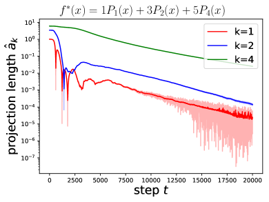
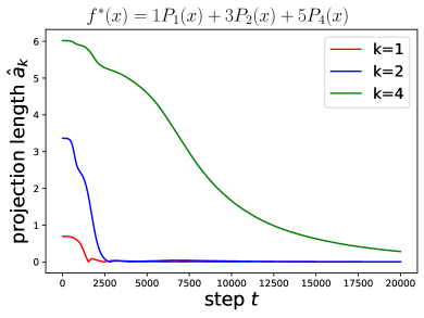
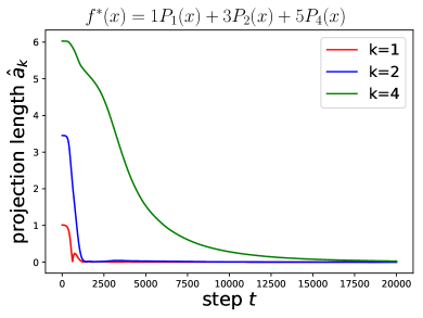
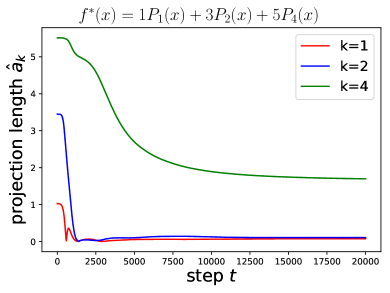
Figure 1: Convergence curve of projection lengths. (a) shows the curve when the target function have the same scale for different components. (b) shows the curve when the higher-order components have larger scale.

The results are shown in Figure 1. It can be seen that the residual at the lowest frequency (k=1𝑘1k=1) converges to zero first and then the second lowest (k=2𝑘2k=2). The highest frequency component is the last one to converge. Following the setting of Rahaman et al. (2019) we assign high frequencies a larger scale in Figure 1 (b), expecting that larger scale will introduce a better descending speed. Still, the low frequencies are learned first.

Note that a^ksubscript^𝑎𝑘\widehat{a}_{k} is the projection length onto an approximate vector. In the function space, we can also project the residual function r(𝐱)=f(𝐱)θf𝐖(t)(𝐱)𝑟𝐱superscript𝑓𝐱𝜃subscript𝑓superscript𝐖𝑡𝐱r(\mathbf{x})=f^{*}(\mathbf{x})-\theta f_{\mathbf{W}^{(t)}}(\mathbf{x}) onto the orthonormal Gegenbauer functions Pk(𝐱)subscript𝑃𝑘𝐱P_{k}(\mathbf{x}). Replacing the training data with randomly sampled data points 𝐱isubscript𝐱𝑖\mathbf{x}_{i} can lead to a random estimate of the projection length in function space. Experiments in this setting can be found in the appendix.

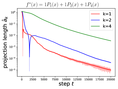
We also verify the linear convergence rate proved in Theorem 4.2. Figure 2 presents the convergence curve in logarithmic scale. We can see from Figure 2 that the convergence of different projection length is close to linear convergence, which is well-aligned with our theoretical analysis. Note that we performed a moving average of range 202020 on these curves to avoid the heavy oscillation especially at late stage.
Refer to caption
(a) same scale
Refer to caption
(b) different scale
Figure 2: Log-scale convergence curve for projection lengths. (a) shows the curve when the target function have the same scale for different components. (b) shows the curve when the higher-order components have larger scale.

5.2 Learning Functions of Simple Forms

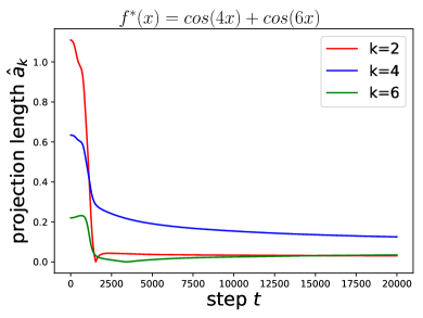
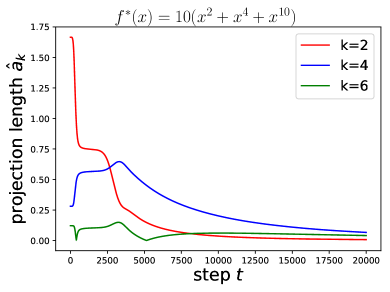
Apart from the synthesized low frequency function, we also show the dynamics of more general functions’ projection to Pk(x)subscript𝑃𝑘𝑥P_{k}(x). These functions, though in a simple form, have non-zero high-frequency components. In this subsection we show our results still apply when all frequencies exist in the target functions, which are given by f(𝐱)=icos(ai𝜻,𝐱)superscript𝑓𝐱subscript𝑖subscript𝑎𝑖𝜻𝐱f^{*}(\mathbf{x})=\sum_{i}\cos(a_{i}\langle{\bm{\zeta}},{\mathbf{x}}\rangle) and f(𝐱)=i𝜻,𝐱pisuperscript𝑓𝐱subscript𝑖superscript𝜻𝐱subscript𝑝𝑖f^{*}(\mathbf{x})=\sum_{i}\langle{\bm{\zeta}},{\mathbf{x}}\rangle^{p_{i}}, where 𝜻𝜻\bm{\zeta} is a fixed unit vector.

Figure 3 verifies the result of Theorem 4.2 with more general target functions, and backs up our claim that Theorem 4.2 does not make any assumptions on the target function. Notice that in the early training stage, not all the curves monotonically descend. We believe this is due to the unseen components’ influence on the gradient. Again, as the training proceeds, the residual projections converge at the predicted rates.
Refer to caption
(a) cosine function
Refer to caption
(b) even polynomial
Figure 3: Convergence curve for different components. (a) shows the curve of a trigonometric function. (b) shows the curve of a polynomial with even degrees.

5.3 Non-uniform Input Data Distributions

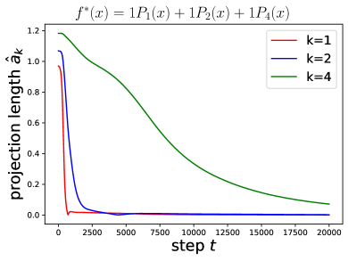
In this subsection, we provide experimental results for non-uniformly distributed input data. Note that the eigendecomposition of NTK for general multi-dimensional input distributions do not necessarily have good analytic forms. Therefore, here we treat the non-uniform distribution of the input data as model misspecification, and test whether residual projections onto spherical harmonics of different degrees can still exhibit various convergence speed. We consider three examples of non-uniform distributions: (i) piece-wise uniform distribution, (ii) normalized non-isotropic Gaussian, and (iii) normalized Gaussian mixture.

Piece-wise uniform distribution We divide the unit sphere into two semi-spheres along a randomly drawn direction 𝜻0subscript𝜻0\bm{\zeta}_{0}. A data input is then generated as follows: with probability 1/4141/4, draw the input uniformly over the first unit sphere; with probability 3/4343/4, draw the input uniformly over the second unit sphere. The results are shown in Figure 4.
Refer to caption
(a) same scale
Refer to caption
(b) different scale
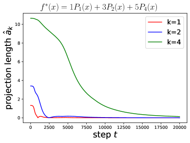
Figure 4: Convergence curve of projection lengths for the piece-wise uniform distribution example.

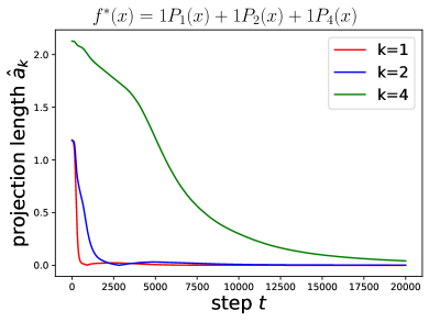
Normalized non-isotropic Gaussian We generate the data by first generating non-zero mean, non-isotropic Gaussian vectors, and then normalize them to unit length. The Gaussian mean vector is generated elementwise from Unif([1,1])Unif11\text{Unif}([-1,1]); the covariance matrix is generated as 𝚺=𝐀𝐀𝚺superscript𝐀top𝐀\bm{\Sigma}=\mathbf{A}^{\top}\mathbf{A}, where 𝐀d×D𝐀subscript𝑑𝐷\mathbf{A}\in\mathbb{R}_{d\times D}(d=10,D=20formulae-sequence𝑑10𝐷20d=10,D=20) has i.i.d. standard Gaussian entries. The results are shown in Figure 5.
Refer to caption
(a) same scale
Refer to caption
(b) different scale
Figure 5: Convergence curve for projection lengths for the normalized non-isotropic Gaussian example.

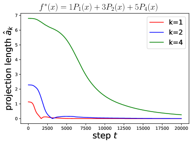
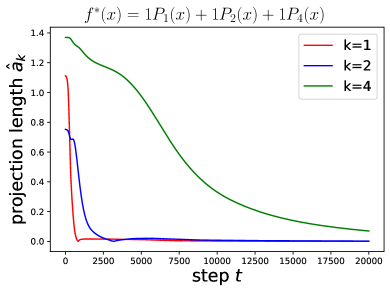
Normalized Gaussian mixture The inputs are drawn from a mixture of 3 non-isotropic Gaussian distributions described above in the second example. The results are shown in Figure 6.

Figures 4, 5, 6 show that the residual components corresponding to lower order polynomials are still learned relatively faster, even for the non-uniform distributions described above, where spherical harmonics are no longer exactly the eigenfunctions of NTK. This suggests that our theoretical results can tolerate certain level of model misspecification, and therefore the spectral bias characterized in Theorem 4.2 and Corollaries 4.6, 4.7 holds in a variety of problem settings.
Refer to caption
(a) same scale
Refer to caption
(b) different scale
Figure 6: Convergence curve of projection lengths for the normalized Gaussian mixture example.

6 Conclusion

In this paper, we give theoretical justification for spectral bias through a detailed analysis of the convergence behavior of two-layer ReLU networks. We show that the convergence of gradient descent in different directions depends on the corresponding eigenvalues and essentially exhibits different convergence rates. We show Mercer decomposition of neural tangent kernel and give explicit order of eigenvalues of integral operator with respect to the neural tangent kernel when the data is uniformly distributed on the unit sphere 𝕊dsuperscript𝕊𝑑\mathbb{S}^{d}. Combined with the convergence analysis, we give the exact order of convergence rate on different directions. We also conduct experiments on synthetic data to support our theoretical result.

Appendix A Appendix A: A Review on Spherical Harmonics

In this section, we give a brief review on relevant concepts in spherical harmonics. For more detials, see Bach (2017); Bietti and Mairal (2019); Frye and Efthimiou (2012); Atkinson and Han (2012) for references.

We consider the unit sphere 𝕊d={𝐱d+1:𝐱2=1}superscript𝕊𝑑conditional-set𝐱superscript𝑑1subscriptnorm𝐱21\mathbb{S}^{d}=\left\{\mathbf{x}\in\mathbb{R}^{d+1}:\|\mathbf{x}\|_{2}=1\right\}, whose surface area is given by ωd=2π(d+1)/2/Γ((d+1)/2)subscript𝜔𝑑2superscript𝜋𝑑12Γ𝑑12\omega_{d}=2\pi^{(d+1)/2}/\Gamma((d+1)/2) and denote τdsubscript𝜏𝑑\tau_{d} the uniform measure on the sphere. For any k1𝑘1k\geq 1, we consider a set of spherical harmonics

{Yk,j:𝕊d|1jN(d,k)=2k+d1k(k+d2d1)}.conditional-setsubscript𝑌𝑘𝑗superscript𝕊𝑑conditional1𝑗𝑁𝑑𝑘2𝑘𝑑1𝑘binomial𝑘𝑑2𝑑1\left\{Y_{k,j}:\mathbb{S}^{d}\rightarrow\mathbb{R}|1\leq j\leq N(d,k)=\frac{2k+d-1}{k}{\binom{k+d-2}{d-1}}\right\}.

They form an orthonormal basis and satisfy the following equation Yki,Ysj𝕊d=𝕊dYki(x)Ysj(x)𝑑τd(x)=δijδsksubscriptsubscript𝑌𝑘𝑖subscript𝑌𝑠𝑗superscript𝕊𝑑subscriptsuperscript𝕊𝑑subscript𝑌𝑘𝑖𝑥subscript𝑌𝑠𝑗𝑥differential-dsubscript𝜏𝑑𝑥subscript𝛿𝑖𝑗subscript𝛿𝑠𝑘\langle Y_{ki},Y_{sj}\rangle_{\mathbb{S}^{d}}=\int_{\mathbb{S}^{d}}Y_{ki}(x)Y_{sj}(x)d\tau_{d}(x)=\delta_{ij}\delta_{sk}. Moreover, since they are homogeneous functions of degree k𝑘k, it is clear that Yk(x)subscript𝑌𝑘𝑥Y_{k}(x) has the same parity as k𝑘k.

We have the addition formula

j=1N(d,k)Yk,j(𝐱)Yk,j(𝐲)=N(d,k)Pk(𝐱,𝐲),superscriptsubscript𝑗1𝑁𝑑𝑘subscript𝑌𝑘𝑗𝐱subscript𝑌𝑘𝑗𝐲𝑁𝑑𝑘subscript𝑃𝑘𝐱𝐲\displaystyle\sum_{j=1}^{N(d,k)}Y_{k,j}(\mathbf{x})Y_{k,j}(\mathbf{y})=N(d,k)P_{k}(\langle{\mathbf{x}},{\mathbf{y}}\rangle), (A.1)

where Pk(t)subscript𝑃𝑘𝑡P_{k}(t) is the Legendre polynomial of degree k𝑘k in d+1𝑑1d+1 dimensions, explicitly given by (Rodrigues’ formula)

Pk(t)=(12)kΓ(d2)Γ(k+d2)(1t2)2d2(ddt)k(1t2)k+d22.subscript𝑃𝑘𝑡superscript12𝑘Γ𝑑2Γ𝑘𝑑2superscript1superscript𝑡22𝑑2superscript𝑑𝑑𝑡𝑘superscript1superscript𝑡2𝑘𝑑22\displaystyle P_{k}(t)=\left(-\frac{1}{2}\right)^{k}\frac{\Gamma\left(\frac{d}{2}\right)}{\Gamma\left(k+\frac{d}{2}\right)}\left(1-t^{2}\right)^{\frac{2-d}{2}}\left(\frac{d}{dt}\right)^{k}\left(1-t^{2}\right)^{k+\frac{d-2}{2}}.

We can also see that Pk(t)subscript𝑃𝑘𝑡P_{k}(t), the Legendre polynomial of degree k𝑘k shares the same parity with k𝑘k. By the orthogonality and the addition formula (A.1) we have,

𝕊dPj(𝐰,𝐱)Pk(𝐰,𝐲)𝑑τd(𝐰)=δjkN(d,k)Pk(𝐱,𝐲).subscriptsuperscript𝕊𝑑subscript𝑃𝑗𝐰𝐱subscript𝑃𝑘𝐰𝐲differential-dsubscript𝜏𝑑𝐰subscript𝛿𝑗𝑘𝑁𝑑𝑘subscript𝑃𝑘𝐱𝐲\displaystyle\int_{\mathbb{S}^{d}}P_{j}(\langle{\mathbf{w}},{\mathbf{x}}\rangle)P_{k}(\langle{\mathbf{w}},{\mathbf{y}}\rangle)d\tau_{d}(\mathbf{w})=\frac{\delta_{jk}}{N(d,k)}P_{k}(\langle{\mathbf{x}},{\mathbf{y}}\rangle). (A.2)

The following recurrence relation holds for Legendre polynomials:

tPk(t)=k2k+d1Pk1(t)+k+d12k+d1Pk+1(t),𝑡subscript𝑃𝑘𝑡𝑘2𝑘𝑑1subscript𝑃𝑘1𝑡𝑘𝑑12𝑘𝑑1subscript𝑃𝑘1𝑡\displaystyle tP_{k}(t)=\frac{k}{2k+d-1}P_{k-1}(t)+\frac{k+d-1}{2k+d-1}P_{k+1}(t), (A.3)

for k1𝑘1k\geq 1 and tP0(t)=P1(t)𝑡subscript𝑃0𝑡subscript𝑃1𝑡tP_{0}(t)=P_{1}(t) for k=0𝑘0k=0.

The Hecke-Funk formula is given for a spherical harmonic Yksubscript𝑌𝑘Y_{k} of degree k𝑘k as follows.

𝕊df(𝐱,𝐲)Yk(𝐲)𝑑τd(𝐲)=ωd1ωdYk(𝐱)11f(t)Pk(t)(1t2)(d2)/2𝑑t.subscriptsuperscript𝕊𝑑𝑓𝐱𝐲subscript𝑌𝑘𝐲differential-dsubscript𝜏𝑑𝐲subscript𝜔𝑑1subscript𝜔𝑑subscript𝑌𝑘𝐱superscriptsubscript11𝑓𝑡subscript𝑃𝑘𝑡superscript1superscript𝑡2𝑑22differential-d𝑡\displaystyle\int_{\mathbb{S}^{d}}f(\langle{\mathbf{x}},{\mathbf{y}}\rangle)Y_{k}(\mathbf{y})d\tau_{d}(\mathbf{y})=\frac{\omega_{d-1}}{\omega_{d}}Y_{k}(\mathbf{x})\int_{-1}^{1}f(t)P_{k}(t)(1-t^{2})^{(d-2)/2}dt. (A.4)

Appendix B Appendix B: Proof of Main Theorems

B.1 Proof of Lemma 4.1

Here we provide the proof of Lemma 4.1, which is based on direct application of concentration inequalities.

Proof of Lemma 4.1.

By definition, we have

(𝐕rk𝐕rk)ij=𝐯i𝐯j=1ns=1nϕi(𝐱s)ϕj(𝐱s),subscriptsuperscriptsubscript𝐕subscript𝑟𝑘topsubscript𝐕subscript𝑟𝑘𝑖𝑗superscriptsubscript𝐯𝑖topsubscript𝐯𝑗1𝑛superscriptsubscript𝑠1𝑛subscriptitalic-ϕ𝑖subscript𝐱𝑠subscriptitalic-ϕ𝑗subscript𝐱𝑠\displaystyle(\mathbf{V}_{r_{k}}^{\top}\mathbf{V}_{r_{k}})_{ij}=\mathbf{v}_{i}^{\top}\mathbf{v}_{j}=\frac{1}{n}\sum_{s=1}^{n}\phi_{i}(\mathbf{x}_{s})\phi_{j}(\mathbf{x}_{s}),

where 𝐱1,𝐱nsubscript𝐱1subscript𝐱𝑛\mathbf{x}_{1},\ldots\mathbf{x}_{n} are i.i.d. samples from distribution τ𝜏\tau. Note that ϕi(𝐱)subscriptitalic-ϕ𝑖𝐱\phi_{i}(\mathbf{x})’s are orthonormal functions in Lτ2(𝕊d)superscriptsubscript𝐿𝜏2superscript𝕊𝑑L_{\tau}^{2}(\mathbb{S}^{d}). By definition we have

𝔼[1ns=1nϕi(𝐱s)ϕj(𝐱s)]=ϕi(𝐱)ϕj(𝐱)𝑑τ(𝐱)=δi,j,𝔼delimited-[]1𝑛superscriptsubscript𝑠1𝑛subscriptitalic-ϕ𝑖subscript𝐱𝑠subscriptitalic-ϕ𝑗subscript𝐱𝑠subscriptitalic-ϕ𝑖𝐱subscriptitalic-ϕ𝑗𝐱differential-d𝜏𝐱subscript𝛿𝑖𝑗\displaystyle\mathbb{E}\Bigg{[}\frac{1}{n}\sum_{s=1}^{n}\phi_{i}(\mathbf{x}_{s})\phi_{j}(\mathbf{x}_{s})\Bigg{]}=\int\phi_{i}(\mathbf{x})\phi_{j}(\mathbf{x})d\tau(\mathbf{x})=\delta_{i,j},

where δi,j=1subscript𝛿𝑖𝑗1\delta_{i,j}=1 if i=j𝑖𝑗i=j and δi,j=0subscript𝛿𝑖𝑗0\delta_{i,j}=0 otherwise. Now since ϕi(𝐱)Msubscriptitalic-ϕ𝑖𝐱𝑀\phi_{i}(\mathbf{x})\leq M for all 𝐱𝕊d𝐱superscript𝕊𝑑\mathbf{x}\in\mathbb{S}^{d} and i[rk]𝑖delimited-[]subscript𝑟𝑘i\in[r_{k}], by standard Hoeffding’s inequality (see Proposition 5.10 in Vershynin (2010)), with probability at least 1δ/rk21𝛿superscriptsubscript𝑟𝑘21-\delta/r_{k}^{2} we have

|(𝐕rk𝐕rk)ijδi,j|C1M2log(rk2/δ)nC2M2log(rk/δ)n,subscriptsuperscriptsubscript𝐕subscript𝑟𝑘topsubscript𝐕subscript𝑟𝑘𝑖𝑗subscript𝛿𝑖𝑗subscript𝐶1superscript𝑀2superscriptsubscript𝑟𝑘2𝛿𝑛subscript𝐶2superscript𝑀2subscript𝑟𝑘𝛿𝑛\displaystyle\big{|}(\mathbf{V}_{r_{k}}^{\top}\mathbf{V}_{r_{k}})_{ij}-\delta_{i,j}\big{|}\leq C_{1}M^{2}\sqrt{\frac{\log(r_{k}^{2}/\delta)}{n}}\leq C_{2}M^{2}\sqrt{\frac{\log(r_{k}/\delta)}{n}},

where C1,C2subscript𝐶1subscript𝐶2C_{1},C_{2} are absolute constants. Applying a union bound over all i,j[rk]×[rk]𝑖𝑗delimited-[]subscript𝑟𝑘delimited-[]subscript𝑟𝑘i,j\in[r_{k}]\times[r_{k}] finishes the proof. ∎

B.2 Proof of Theorem 4.2

In this section we give the proof of Theorem 4.2. The core idea of our proof is to establish connections between neural network gradients throughout training and the neural tangent kernel. To do so, we first introduce the following definitions and notations.

Define 𝐊(0)=m1(𝐖f𝐖(0)(𝐱i),𝐖f𝐖(0)(𝐱j))n×nsuperscript𝐊0superscript𝑚1subscriptsubscript𝐖subscript𝑓superscript𝐖0subscript𝐱𝑖subscript𝐖subscript𝑓superscript𝐖0subscript𝐱𝑗𝑛𝑛\mathbf{K}^{(0)}=m^{-1}(\langle\nabla_{\mathbf{W}}f_{\mathbf{W}^{(0)}}(\mathbf{x}_{i}),\nabla_{\mathbf{W}}f_{\mathbf{W}^{(0)}}(\mathbf{x}_{j})\rangle)_{n\times n}, 𝐊()=(κ(𝐱i,𝐱j))n×n=limm𝐊(0)superscript𝐊subscript𝜅subscript𝐱𝑖subscript𝐱𝑗𝑛𝑛subscript𝑚superscript𝐊0\mathbf{K}^{(\infty)}=(\kappa(\mathbf{x}_{i},\mathbf{x}_{j}))_{n\times n}=\lim_{m\rightarrow\infty}\mathbf{K}^{(0)}. Let {λ^i}i=1nsuperscriptsubscriptsubscript^𝜆𝑖𝑖1𝑛\{\widehat{\lambda}_{i}\}_{i=1}^{n}, λ^1λ^nsubscript^𝜆1subscript^𝜆𝑛\widehat{\lambda}_{1}\geq\cdots\geq\widehat{\lambda}_{n} be the eigenvalues of n1𝐊superscript𝑛1superscript𝐊n^{-1}\mathbf{K}^{\infty}, and 𝐯^1,,𝐯^nsubscript^𝐯1subscript^𝐯𝑛\widehat{\mathbf{v}}_{1},\ldots,\widehat{\mathbf{v}}_{n} be the corresponding eigenvectors. Set 𝐕^rk=(𝐯^1,,𝐯^rk)subscript^𝐕subscript𝑟𝑘subscript^𝐯1subscript^𝐯subscript𝑟𝑘\widehat{\mathbf{V}}_{{r_{k}}}=(\widehat{\mathbf{v}}_{1},\ldots,\widehat{\mathbf{v}}_{{r_{k}}}), 𝐕^rk=(𝐯^rk+1,,𝐯^n)superscriptsubscript^𝐕subscript𝑟𝑘bottomsubscript^𝐯subscript𝑟𝑘1subscript^𝐯𝑛\widehat{\mathbf{V}}_{{r_{k}}}^{\bot}=(\widehat{\mathbf{v}}_{{r_{k}}+1},\ldots,\widehat{\mathbf{v}}_{n}). For notation simplicity, we denote 𝐖f𝐖(0)(𝐱i)=[𝐖f𝐖(𝐱i)]|𝐖=𝐖(0)subscript𝐖subscript𝑓superscript𝐖0subscript𝐱𝑖evaluated-atdelimited-[]subscript𝐖subscript𝑓𝐖subscript𝐱𝑖𝐖superscript𝐖0\nabla_{\mathbf{W}}f_{\mathbf{W}^{(0)}}(\mathbf{x}_{i})=[\nabla_{\mathbf{W}}f_{\mathbf{W}}(\mathbf{x}_{i})]\big{|}_{\mathbf{W}=\mathbf{W}^{(0)}}, 𝐖lf𝐖(0)(𝐱i)=[𝐖lf𝐖(𝐱i)]|𝐖=𝐖(0)subscriptsubscript𝐖𝑙subscript𝑓superscript𝐖0subscript𝐱𝑖evaluated-atdelimited-[]subscriptsubscript𝐖𝑙subscript𝑓𝐖subscript𝐱𝑖𝐖superscript𝐖0\nabla_{\mathbf{W}_{l}}f_{\mathbf{W}^{(0)}}(\mathbf{x}_{i})=[\nabla_{\mathbf{W}_{l}}f_{\mathbf{W}}(\mathbf{x}_{i})]\big{|}_{\mathbf{W}=\mathbf{W}^{(0)}}, l=1,2𝑙12l=1,2.

The following lemma’s purpose is to further connect the eigenfunctions of NTK with their finite-width, finite-sample counterparts. Its first statement is proved in Su and Yang (2019).

Lemma B.1.

Suppose that |ϕi(𝐱)|Msubscriptitalic-ϕ𝑖𝐱𝑀|\phi_{i}(\mathbf{x})|\leq M for all 𝐱Sd𝐱superscript𝑆𝑑\mathbf{x}\in S^{d}. There exist absolute constants C,C,c′′>0𝐶superscript𝐶superscript𝑐′′0C,C^{\prime},c^{\prime\prime}>0, such that for any δ>0𝛿0\delta>0 and integer k𝑘k with rknsubscript𝑟𝑘𝑛{r_{k}}\leq n, if nC(λrkλrk+1)2log(1/δ)𝑛𝐶superscriptsubscript𝜆subscript𝑟𝑘subscript𝜆subscript𝑟𝑘121𝛿n\geq C(\lambda_{{r_{k}}}-\lambda_{{r_{k}}+1})^{-2}\log(1/\delta), then with probability at least 1δ1𝛿1-\delta,

𝐕rk𝐕^rkFC1λrkλrk+1log(1/δ)n,subscriptnormsuperscriptsubscript𝐕subscript𝑟𝑘topsuperscriptsubscript^𝐕subscript𝑟𝑘bottom𝐹superscript𝐶1subscript𝜆subscript𝑟𝑘subscript𝜆subscript𝑟𝑘11𝛿𝑛\displaystyle\|\mathbf{V}_{{r_{k}}}^{\top}\widehat{\mathbf{V}}_{{r_{k}}}^{\bot}\|_{F}\leq C^{\prime}\frac{1}{\lambda_{r_{k}}-\lambda_{r_{k}+1}}\cdot\sqrt{\frac{\log(1/\delta)}{n}},
𝐕rk𝐕rk𝐕^rk𝐕^rk2C′′[1λrkλrk+1log(1/δ)n+M2rklog(rk/δ)n].subscriptnormsubscript𝐕subscript𝑟𝑘superscriptsubscript𝐕subscript𝑟𝑘topsubscript^𝐕subscript𝑟𝑘superscriptsubscript^𝐕subscript𝑟𝑘top2superscript𝐶′′delimited-[]1subscript𝜆subscript𝑟𝑘subscript𝜆subscript𝑟𝑘11𝛿𝑛superscript𝑀2subscript𝑟𝑘subscript𝑟𝑘𝛿𝑛\displaystyle\|\mathbf{V}_{{r_{k}}}\mathbf{V}_{{r_{k}}}^{\top}-\widehat{\mathbf{V}}_{{r_{k}}}\widehat{\mathbf{V}}_{{r_{k}}}^{\top}\|_{2}\leq C^{\prime\prime}\bigg{[}\frac{1}{\lambda_{r_{k}}-\lambda_{r_{k}+1}}\cdot\sqrt{\frac{\log(1/\delta)}{n}}+M^{2}r_{k}\sqrt{\frac{\log(r_{k}/\delta)}{n}}\bigg{]}.

The following two lemmas gives some preliminary bounds on the function value and gradients of the neural network around random initialization. They are proved in Cao and Gu (2019).

Lemma B.2 (Cao and Gu (2019)).

For any δ>0𝛿0\delta>0, if mClog(n/δ)𝑚𝐶𝑛𝛿m\geq C\log(n/\delta) for a large enough absolute constant C𝐶C, then with probability at least 1δ1𝛿1-\delta, |f𝐖(0)(𝒙i)|𝒪(log(n/δ))subscript𝑓superscript𝐖0subscript𝒙𝑖𝒪𝑛𝛿|f_{\mathbf{W}^{(0)}}(\bm{x}_{i})|\leq\mathcal{O}(\sqrt{\log(n/\delta)}) for all i[n]𝑖delimited-[]𝑛i\in[n].

Lemma B.3 (Cao and Gu (2019)).

There exists an absolute constant C𝐶C such that, with probability at least 1𝒪(n)exp[Ω(mω2/3)]1𝒪𝑛Ω𝑚superscript𝜔231-\mathcal{O}(n)\cdot\exp[-\Omega(m\omega^{2/3})], for all i[n]𝑖delimited-[]𝑛i\in[n], l[L]𝑙delimited-[]𝐿l\in[L] and 𝐖(𝐖(0),ω)𝐖superscript𝐖0𝜔\mathbf{W}\in\mathcal{B}(\mathbf{W}^{(0)},\omega) with ωC[log(m)]3𝜔𝐶superscriptdelimited-[]𝑚3\omega\leq C[\log(m)]^{-3}, it holds uniformly that

𝐖lf𝐖(𝐱i)F𝒪(m).subscriptnormsubscriptsubscript𝐖𝑙subscript𝑓𝐖subscript𝐱𝑖𝐹𝒪𝑚\displaystyle\|\nabla_{\mathbf{W}_{l}}f_{\mathbf{W}}(\mathbf{x}_{i})\|_{F}\leq\mathcal{O}(\sqrt{m}).

The following lemma is the key to characterize the dynamics of the residual throughout training. These bounds in Lemma B.4 are the ones that distinguish our analysis from previous works on neural network training in the NTK regime (Du et al., 2019b; Su and Yang, 2019), since our analysis provides more careful characterization on the residual along different directions.

Lemma B.4.

Suppose that the iterates of gradient descent 𝐖(0),,𝐖(t)superscript𝐖0superscript𝐖𝑡\mathbf{W}^{(0)},\ldots,\mathbf{W}^{(t)} are inside the ball (𝐖(0),ω)superscript𝐖0𝜔\mathcal{B}(\mathbf{W}^{(0)},\omega). If ω𝒪~(min{[log(m)]3/2,λrk3,(ηm)3})𝜔~𝒪superscriptdelimited-[]𝑚32superscriptsubscript𝜆subscript𝑟𝑘3superscript𝜂𝑚3\omega\leq\widetilde{\mathcal{O}}(\min\{[\log(m)]^{-3/2},\lambda_{r_{k}}^{3},(\eta m)^{-3}\}) and n𝒪~(λrk2)𝑛~𝒪superscriptsubscript𝜆subscript𝑟𝑘2n\geq\widetilde{\mathcal{O}}(\lambda_{r_{k}}^{-2}), then with probability at least 1𝒪(t2n2)exp[Ω(mω2/3)]1𝒪superscript𝑡2superscript𝑛2Ω𝑚superscript𝜔231-\mathcal{O}(t^{2}n^{2})\cdot\exp[-\Omega(m\omega^{2/3})],

(𝐕^rk)(𝐲𝐲^(t))2subscriptnormsuperscriptsuperscriptsubscript^𝐕subscript𝑟𝑘bottomtop𝐲superscript^𝐲superscript𝑡2\displaystyle\|(\widehat{\mathbf{V}}_{r_{k}}^{\bot})^{\top}(\mathbf{y}-\widehat{\mathbf{y}}^{({t^{\prime}})})\|_{2} (𝐕^rk)(𝐲𝐲^(0))2+tω1/3ηmθ2n𝒪~(1+ωm)absentsubscriptnormsuperscriptsuperscriptsubscript^𝐕subscript𝑟𝑘bottomtop𝐲superscript^𝐲02superscript𝑡superscript𝜔13𝜂𝑚superscript𝜃2𝑛~𝒪1𝜔𝑚\displaystyle\leq\|(\widehat{\mathbf{V}}_{r_{k}}^{\bot})^{\top}(\mathbf{y}-\widehat{\mathbf{y}}^{(0)})\|_{2}+{t^{\prime}}\cdot\omega^{1/3}\eta m\theta^{2}\cdot\sqrt{n}\cdot\widetilde{\mathcal{O}}(1+\omega\sqrt{m}) (B.1)
𝐕^rk(𝐲𝐲^(t))2subscriptnormsuperscriptsubscript^𝐕subscript𝑟𝑘top𝐲superscript^𝐲superscript𝑡2\displaystyle\|\widehat{\mathbf{V}}_{r_{k}}^{\top}(\mathbf{y}-\widehat{\mathbf{y}}^{({t^{\prime}})})\|_{2} (1ηmθ2λrk/2)t𝐕^rk(𝐲𝐲^(0))2+tλrk1ω2/3ηmθ2n𝒪~(1+ωm)absentsuperscript1𝜂𝑚superscript𝜃2subscript𝜆subscript𝑟𝑘2superscript𝑡subscriptnormsuperscriptsubscript^𝐕subscript𝑟𝑘top𝐲superscript^𝐲02superscript𝑡superscriptsubscript𝜆subscript𝑟𝑘1superscript𝜔23𝜂𝑚superscript𝜃2𝑛~𝒪1𝜔𝑚\displaystyle\leq(1-\eta m\theta^{2}\lambda_{r_{k}}/2)^{t^{\prime}}\|\widehat{\mathbf{V}}_{r_{k}}^{\top}(\mathbf{y}-\widehat{\mathbf{y}}^{(0)})\|_{2}+{t^{\prime}}\lambda_{r_{k}}^{-1}\cdot\omega^{2/3}\eta m\theta^{2}\cdot\sqrt{n}\cdot\widetilde{\mathcal{O}}(1+\omega\sqrt{m})
+λrk1𝒪~(ω1/3)(𝐕^rk)(𝐲𝐲^(0))2superscriptsubscript𝜆subscript𝑟𝑘1~𝒪superscript𝜔13subscriptnormsuperscriptsuperscriptsubscript^𝐕subscript𝑟𝑘bottomtop𝐲superscript^𝐲02\displaystyle\quad+\lambda_{r_{k}}^{-1}\cdot\widetilde{\mathcal{O}}(\omega^{1/3})\cdot\|(\widehat{\mathbf{V}}_{r_{k}}^{\bot})^{\top}(\mathbf{y}-\widehat{\mathbf{y}}^{(0)})\|_{2} (B.2)
𝐲𝐲^(t)2subscriptnorm𝐲superscript^𝐲superscript𝑡2\displaystyle\|\mathbf{y}-\widehat{\mathbf{y}}^{({t^{\prime}})}\|_{2} 𝒪~(n)(1ηmθ2λrk/2)t+𝒪~(n(ηmθ2λrk)1)absent~𝒪𝑛superscript1𝜂𝑚superscript𝜃2subscript𝜆subscript𝑟𝑘2superscript𝑡~𝒪𝑛superscript𝜂𝑚superscript𝜃2subscript𝜆subscript𝑟𝑘1\displaystyle\leq\widetilde{\mathcal{O}}(\sqrt{n})\cdot(1-\eta m\theta^{2}\lambda_{r_{k}}/2)^{t^{\prime}}+\widetilde{\mathcal{O}}(\sqrt{n}\cdot(\eta m\theta^{2}\lambda_{r_{k}})^{-1})
+λrk1tω1/3n𝒪~(1+ωm)superscriptsubscript𝜆subscript𝑟𝑘1superscript𝑡superscript𝜔13𝑛~𝒪1𝜔𝑚\displaystyle\quad+\lambda_{r_{k}}^{-1}{t^{\prime}}\omega^{1/3}\cdot\sqrt{n}\cdot\widetilde{\mathcal{O}}(1+\omega\sqrt{m}) (B.3)

for all t=0,,t1superscript𝑡0𝑡1{t^{\prime}}=0,\ldots,t-1.

Now we are ready to prove Theorem 4.2. To illustrate the intuition behind the proof, the proof can be mainly summarized into three steps: (i) Using a induction argument together with Lemma B.4 to show that under the theorem assumptions, all T𝑇T gradient descent iterates 𝐖(0),,𝐖(T)superscript𝐖0superscript𝐖𝑇\mathbf{W}^{(0)},\ldots,\mathbf{W}^{(T)} are inside the ball (𝐖(0),ω)superscript𝐖0𝜔\mathcal{B}(\mathbf{W}^{(0)},\omega) with ω=O(T/(𝜽λrkm))𝜔𝑂𝑇𝜽subscript𝜆subscript𝑟𝑘𝑚\omega=O(T/(\bm{\theta}\lambda_{r_{k}}\sqrt{m})). (ii) We then reapply Lemma B.4 with t=T𝑡𝑇t=T and obtain a bound on 𝐕^rk(𝐲𝐲^(T))2subscriptnormsuperscriptsubscript^𝐕subscript𝑟𝑘top𝐲superscript^𝐲𝑇2\|\widehat{\mathbf{V}}_{r_{k}}^{\top}(\mathbf{y}-\widehat{\mathbf{y}}^{(T)})\|_{2}. (iii) At last, we utilize the concentration results given in Lemma B.1 to finalize the proof. The detaled proof is given as follows.

Proof of Theorem 4.2.

Define ω=C¯T/(𝜽λrkm)𝜔¯𝐶𝑇𝜽subscript𝜆subscript𝑟𝑘𝑚\omega=\overline{C}T/(\bm{\theta}\lambda_{r_{k}}\sqrt{m}) for some small enough absolute constant C¯¯𝐶\overline{C}. Then by union bound, as long as mΩ~(poly(T,λrk1,ϵ1))𝑚~Ωpoly𝑇superscriptsubscript𝜆subscript𝑟𝑘1superscriptitalic-ϵ1m\geq\widetilde{\Omega}(\mathrm{poly}(T,\lambda_{r_{k}}^{-1},\epsilon^{-1})), the conditions on ω𝜔\omega given in Lemmas B.3 and B.4 are satisfied.

We first show that all the iterates 𝐖(0),,𝐖(T)superscript𝐖0superscript𝐖𝑇\mathbf{W}^{(0)},\ldots,\mathbf{W}^{(T)} are inside the ball (𝐖(0),ω)superscript𝐖0𝜔\mathcal{B}(\mathbf{W}^{(0)},\omega). We prove this result by inductively show that 𝐖(t)(𝐖(0),ω)superscript𝐖𝑡superscript𝐖0𝜔\mathbf{W}^{(t)}\in\mathcal{B}(\mathbf{W}^{(0)},\omega), t=0,,T𝑡0𝑇t=0,\ldots,T. First of all, it is clear that 𝐖(0)(𝐖(0),ω)superscript𝐖0superscript𝐖0𝜔\mathbf{W}^{(0)}\in\mathcal{B}(\mathbf{W}^{(0)},\omega). Suppose that 𝐖(0),,𝐖(t)(𝐖(0),ω)superscript𝐖0superscript𝐖𝑡superscript𝐖0𝜔\mathbf{W}^{(0)},\ldots,\mathbf{W}^{(t)}\in\mathcal{B}(\mathbf{W}^{(0)},\omega). Then the results of Lemmas B.3 and B.4 hold for 𝐖(0),,𝐖(t)superscript𝐖0superscript𝐖𝑡\mathbf{W}^{(0)},\ldots,\mathbf{W}^{(t)}. Denote 𝐮(t)=𝐲𝐲^(t)superscript𝐮𝑡𝐲superscript^𝐲𝑡\mathbf{u}^{(t)}=\mathbf{y}-\widehat{\mathbf{y}}^{(t)}, tT𝑡𝑇t\in{T}. Then we have

𝐖l(t+1)𝐖l(0)Fsubscriptnormsuperscriptsubscript𝐖𝑙𝑡1superscriptsubscript𝐖𝑙0𝐹\displaystyle\|\mathbf{W}_{l}^{(t+1)}-\mathbf{W}_{l}^{(0)}\|_{F} t=0t𝐖l(t+1)𝐖l(t)Fabsentsuperscriptsubscriptsuperscript𝑡0𝑡subscriptnormsuperscriptsubscript𝐖𝑙superscript𝑡1superscriptsubscript𝐖𝑙superscript𝑡𝐹\displaystyle\leq\sum_{{t^{\prime}}=0}^{t}\|\mathbf{W}_{l}^{({t^{\prime}}+1)}-\mathbf{W}_{l}^{({t^{\prime}})}\|_{F}
=ηt=0t1ni=1n(yiθf𝐖(t)(𝐱i))θ𝐖lf𝐖(t)(𝐱i)Fabsent𝜂superscriptsubscriptsuperscript𝑡0𝑡subscriptnorm1𝑛superscriptsubscript𝑖1𝑛subscript𝑦𝑖𝜃subscript𝑓superscript𝐖𝑡subscript𝐱𝑖𝜃subscriptsubscript𝐖𝑙subscript𝑓superscript𝐖𝑡subscript𝐱𝑖𝐹\displaystyle=\eta\sum_{{t^{\prime}}=0}^{t}\Bigg{\|}\frac{1}{n}\sum_{i=1}^{n}(y_{i}-\theta\cdot f_{\mathbf{W}^{(t)}}(\mathbf{x}_{i}))\cdot\theta\cdot\nabla_{\mathbf{W}_{l}}f_{\mathbf{W}^{(t)}}(\mathbf{x}_{i})\Bigg{\|}_{F}
ηθt=0t1ni=1n|yiθf𝐖(t)(𝐱i)|𝐖lf𝐖(t)(𝐱i)Fabsent𝜂𝜃superscriptsubscriptsuperscript𝑡0𝑡1𝑛superscriptsubscript𝑖1𝑛subscript𝑦𝑖𝜃subscript𝑓superscript𝐖𝑡subscript𝐱𝑖subscriptnormsubscriptsubscript𝐖𝑙subscript𝑓superscript𝐖𝑡subscript𝐱𝑖𝐹\displaystyle\leq\eta\theta\sum_{{t^{\prime}}=0}^{t}\frac{1}{n}\sum_{i=1}^{n}|y_{i}-\theta\cdot f_{\mathbf{W}^{(t)}}(\mathbf{x}_{i})|\cdot\|\nabla_{\mathbf{W}_{l}}f_{\mathbf{W}^{(t)}}(\mathbf{x}_{i})\|_{F}
C1ηθmt=0t1ni=1n|yiθf𝐖(t)(𝐱i)|absentsubscript𝐶1𝜂𝜃𝑚superscriptsubscriptsuperscript𝑡0𝑡1𝑛superscriptsubscript𝑖1𝑛subscript𝑦𝑖𝜃subscript𝑓superscript𝐖𝑡subscript𝐱𝑖\displaystyle\leq C_{1}\eta\theta\sqrt{m}\sum_{{t^{\prime}}=0}^{t}\frac{1}{n}\sum_{i=1}^{n}|y_{i}-\theta\cdot f_{\mathbf{W}^{(t)}}(\mathbf{x}_{i})|
C1ηθm/nt=0t𝐲𝐲^(t)2,absentsubscript𝐶1𝜂𝜃𝑚𝑛superscriptsubscriptsuperscript𝑡0𝑡subscriptnorm𝐲superscript^𝐲superscript𝑡2\displaystyle\leq C_{1}\eta\theta\sqrt{m/n}\sum_{{t^{\prime}}=0}^{t}\|\mathbf{y}-\widehat{\mathbf{y}}^{({t^{\prime}})}\|_{2},

where the second inequality follows by Lemma B.3. By Lemma B.4, we have

t=0t𝐲𝐲^(t)2superscriptsubscriptsuperscript𝑡0𝑡subscriptnorm𝐲superscript^𝐲superscript𝑡2\displaystyle\sum_{{t^{\prime}}=0}^{t}\|\mathbf{y}-\widehat{\mathbf{y}}^{({t^{\prime}})}\|_{2} 𝒪~(n/(ηmθ2λrk))+𝒪~(Tn/(ηmθ2λrk))+λrk1T2ω1/3n𝒪~(1+ωm).absent~𝒪𝑛𝜂𝑚superscript𝜃2subscript𝜆subscript𝑟𝑘~𝒪𝑇𝑛𝜂𝑚superscript𝜃2subscript𝜆subscript𝑟𝑘superscriptsubscript𝜆subscript𝑟𝑘1superscript𝑇2superscript𝜔13𝑛~𝒪1𝜔𝑚\displaystyle\leq\widetilde{\mathcal{O}}(\sqrt{n}/(\eta m\theta^{2}\lambda_{r_{k}}))+\widetilde{\mathcal{O}}(T\sqrt{n}/(\eta m\theta^{2}\lambda_{r_{k}}))+\lambda_{r_{k}}^{-1}T^{2}\omega^{1/3}\sqrt{n}\cdot\widetilde{\mathcal{O}}(1+\omega\sqrt{m}).

It then follows by the choice ω=C¯T/(θλrkm)𝜔¯𝐶𝑇𝜃subscript𝜆subscript𝑟𝑘𝑚\omega=\overline{C}T/(\theta\lambda_{r_{k}}\sqrt{m}), η=𝒪~((mθ2)1)𝜂~𝒪superscript𝑚superscript𝜃21\eta=\widetilde{\mathcal{O}}((m\theta^{2})^{-1}), θ=𝒪~(ϵ)𝜃~𝒪italic-ϵ\theta=\widetilde{\mathcal{O}}(\epsilon) and the assumption m𝒪~(poly(T,λrk1,ϵ1))𝑚~𝒪poly𝑇superscriptsubscript𝜆subscript𝑟𝑘1superscriptitalic-ϵ1m\geq\widetilde{\mathcal{O}}(\mathrm{poly}(T,\lambda_{r_{k}}^{-1},\epsilon^{-1})) that 𝐖l(t+1)𝐖l(0)Fωsubscriptnormsuperscriptsubscript𝐖𝑙𝑡1superscriptsubscript𝐖𝑙0𝐹𝜔\|\mathbf{W}_{l}^{(t+1)}-\mathbf{W}_{l}^{(0)}\|_{F}\leq\omega, l=1,2𝑙12l=1,2. Therefore by induction, we see that with probability at least 1𝒪(T3n2)exp[Ω(mω2/3)]1𝒪superscript𝑇3superscript𝑛2Ω𝑚superscript𝜔231-\mathcal{O}(T^{3}n^{2})\cdot\exp[-\Omega(m\omega^{2/3})], 𝐖(0),,𝐖(T)(𝐖(0),ω)𝐖0𝐖𝑇superscript𝐖0𝜔\mathbf{W}{(0)},\ldots,\mathbf{W}{(T)}\in\mathcal{B}(\mathbf{W}^{(0)},\omega) .

Applying Lemma B.4 then gives

n1/2𝐕^rk(𝐲𝐲^(T))2superscript𝑛12subscriptnormsuperscriptsubscript^𝐕subscript𝑟𝑘top𝐲superscript^𝐲𝑇2\displaystyle n^{-1/2}\cdot\|\widehat{\mathbf{V}}_{r_{k}}^{\top}(\mathbf{y}-\widehat{\mathbf{y}}^{(T)})\|_{2} (1ηmθ2λrk/2)Tn1/2𝐕^rk(𝐲𝐲^(0))2absentsuperscript1𝜂𝑚superscript𝜃2subscript𝜆subscript𝑟𝑘2𝑇superscript𝑛12subscriptnormsuperscriptsubscript^𝐕subscript𝑟𝑘top𝐲superscript^𝐲02\displaystyle\leq(1-\eta m\theta^{2}\lambda_{r_{k}}/2)^{T}\cdot n^{-1/2}\cdot\|\widehat{\mathbf{V}}_{r_{k}}^{\top}(\mathbf{y}-\widehat{\mathbf{y}}^{(0)})\|_{2}
+Tλrk1ω2/3ηmθ2𝒪~(1+ωm)𝑇superscriptsubscript𝜆subscript𝑟𝑘1superscript𝜔23𝜂𝑚superscript𝜃2~𝒪1𝜔𝑚\displaystyle\quad+T\lambda_{r_{k}}^{-1}\cdot\omega^{2/3}\eta m\theta^{2}\cdot\widetilde{\mathcal{O}}(1+\omega\sqrt{m})
+λrk1𝒪~(ω1/3)n1/2(𝐕^rk)(𝐲𝐲^(0))2.superscriptsubscript𝜆subscript𝑟𝑘1~𝒪superscript𝜔13superscript𝑛12subscriptnormsuperscriptsuperscriptsubscript^𝐕subscript𝑟𝑘bottomtop𝐲superscript^𝐲02\displaystyle\quad+\lambda_{r_{k}}^{-1}\cdot\widetilde{\mathcal{O}}(\omega^{1/3})\cdot n^{-1/2}\cdot\|(\widehat{\mathbf{V}}_{r_{k}}^{\bot})^{\top}(\mathbf{y}-\widehat{\mathbf{y}}^{(0)})\|_{2}.

Now by ω=C¯T/(λrkm)𝜔¯𝐶𝑇subscript𝜆subscript𝑟𝑘𝑚\omega=\overline{C}T/(\lambda_{r_{k}}\sqrt{m}), η=𝒪~(θ2m)1𝜂~𝒪superscriptsuperscript𝜃2𝑚1\eta=\widetilde{\mathcal{O}}(\theta^{2}m)^{-1} and the assumption that mm=𝒪~(λrk14ϵ6)𝑚superscript𝑚~𝒪superscriptsubscript𝜆subscript𝑟𝑘14superscriptitalic-ϵ6m\geq m^{*}=\widetilde{\mathcal{O}}(\lambda_{r_{k}}^{-14}\cdot\epsilon^{-6}), we obtain

n1/2𝐕^rk(𝐲𝐲^(T))2(1λrk)Tn1/2𝐕^rk(𝐲𝐲^(0))2+ϵ/16.superscript𝑛12subscriptnormsuperscriptsubscript^𝐕subscript𝑟𝑘top𝐲superscript^𝐲𝑇2superscript1subscript𝜆subscript𝑟𝑘𝑇superscript𝑛12subscriptnormsuperscriptsubscript^𝐕subscript𝑟𝑘top𝐲superscript^𝐲02italic-ϵ16\displaystyle n^{-1/2}\cdot\|\widehat{\mathbf{V}}_{r_{k}}^{\top}(\mathbf{y}-\widehat{\mathbf{y}}^{(T)})\|_{2}\leq(1-\lambda_{r_{k}})^{T}\cdot n^{-1/2}\cdot\|\widehat{\mathbf{V}}_{r_{k}}^{\top}(\mathbf{y}-\widehat{\mathbf{y}}^{(0)})\|_{2}+\epsilon/16. (B.4)

By Lemma 4.1, θ=𝒪~(ϵ)𝜃~𝒪italic-ϵ\theta=\widetilde{\mathcal{O}}(\epsilon) and the assumptions nΩ~(max{ϵ1(λrkλrk+1)1,ϵ2M2rk2})𝑛~Ωsuperscriptitalic-ϵ1superscriptsubscript𝜆subscript𝑟𝑘subscript𝜆subscript𝑟𝑘11superscriptitalic-ϵ2superscript𝑀2superscriptsubscript𝑟𝑘2n\geq\widetilde{\Omega}(\max\{\epsilon^{-1}(\lambda_{r_{k}}-\lambda_{r_{k}+1})^{-1},\epsilon^{-2}M^{2}r_{k}^{2}\}), the eigenvalues of 𝐕rk𝐕rksuperscriptsubscript𝐕subscript𝑟𝑘topsubscript𝐕subscript𝑟𝑘\mathbf{V}_{r_{k}}^{\top}\mathbf{V}_{r_{k}} are all between 1/2121/\sqrt{2} and 22\sqrt{2}. Therefore we have

𝐕^rk(𝐲𝐲^(T))2subscriptnormsuperscriptsubscript^𝐕subscript𝑟𝑘top𝐲superscript^𝐲𝑇2\displaystyle\|\widehat{\mathbf{V}}_{r_{k}}^{\top}(\mathbf{y}-\widehat{\mathbf{y}}^{(T)})\|_{2} =𝐕^rk𝐕^rk(𝐲𝐲^(T))2absentsubscriptnormsubscript^𝐕subscript𝑟𝑘superscriptsubscript^𝐕subscript𝑟𝑘top𝐲superscript^𝐲𝑇2\displaystyle=\|\widehat{\mathbf{V}}_{r_{k}}\widehat{\mathbf{V}}_{r_{k}}^{\top}(\mathbf{y}-\widehat{\mathbf{y}}^{(T)})\|_{2}
𝐕rk𝐕rk(𝐲𝐲^(T))2(𝐕rk𝐕rk𝐕^rk𝐕^rk)(𝐲𝐲^(T))2absentsubscriptnormsubscript𝐕subscript𝑟𝑘superscriptsubscript𝐕subscript𝑟𝑘top𝐲superscript^𝐲𝑇2subscriptnormsubscript𝐕subscript𝑟𝑘superscriptsubscript𝐕subscript𝑟𝑘topsubscript^𝐕subscript𝑟𝑘superscriptsubscript^𝐕subscript𝑟𝑘top𝐲superscript^𝐲𝑇2\displaystyle\geq\|\mathbf{V}_{r_{k}}\mathbf{V}_{r_{k}}^{\top}(\mathbf{y}-\widehat{\mathbf{y}}^{(T)})\|_{2}-\|(\mathbf{V}_{r_{k}}\mathbf{V}_{r_{k}}^{\top}-\widehat{\mathbf{V}}_{r_{k}}\widehat{\mathbf{V}}_{r_{k}}^{\top})(\mathbf{y}-\widehat{\mathbf{y}}^{(T)})\|_{2}
𝐕rk(𝐲𝐲^(T))2/2n𝒪(1λrkλrk+1log(1/δ)n+Mrklog(rk/δ)n)absentsubscriptnormsuperscriptsubscript𝐕subscript𝑟𝑘top𝐲superscript^𝐲𝑇22𝑛𝒪1subscript𝜆subscript𝑟𝑘subscript𝜆subscript𝑟𝑘11𝛿𝑛𝑀subscript𝑟𝑘subscript𝑟𝑘𝛿𝑛\displaystyle\geq\|\mathbf{V}_{r_{k}}^{\top}(\mathbf{y}-\widehat{\mathbf{y}}^{(T)})\|_{2}/\sqrt{2}-\sqrt{n}\cdot\mathcal{O}\bigg{(}\frac{1}{\lambda_{r_{k}}-\lambda_{r_{k}+1}}\cdot\sqrt{\frac{\log(1/\delta)}{n}}+Mr_{k}\sqrt{\frac{\log(r_{k}/\delta)}{n}}\bigg{)}
𝐕rk(𝐲𝐲^(T))2/2ϵn/16,absentsubscriptnormsuperscriptsubscript𝐕subscript𝑟𝑘top𝐲superscript^𝐲𝑇22italic-ϵ𝑛16\displaystyle\geq\|\mathbf{V}_{r_{k}}^{\top}(\mathbf{y}-\widehat{\mathbf{y}}^{(T)})\|_{2}/\sqrt{2}-\epsilon\sqrt{n}/16,

where the second inequality follows by Lemma B.1 and the fact 𝐕rk𝐕rk(1/2)𝐈succeeds-or-equalssuperscriptsubscript𝐕subscript𝑟𝑘topsubscript𝐕subscript𝑟𝑘12𝐈\mathbf{V}_{r_{k}}^{\top}\mathbf{V}_{r_{k}}\succeq(1/\sqrt{2})\mathbf{I}. Similarly,

𝐕^rk(𝐲𝐲^(0))2subscriptnormsuperscriptsubscript^𝐕subscript𝑟𝑘top𝐲superscript^𝐲02\displaystyle\|\widehat{\mathbf{V}}_{r_{k}}^{\top}(\mathbf{y}-\widehat{\mathbf{y}}^{(0)})\|_{2} 2𝐕rk(𝐲𝐲^(0))2+ϵn/16absent2subscriptnormsuperscriptsubscript𝐕subscript𝑟𝑘top𝐲superscript^𝐲02italic-ϵ𝑛16\displaystyle\leq\sqrt{2}\cdot\|\mathbf{V}_{r_{k}}^{\top}(\mathbf{y}-\widehat{\mathbf{y}}^{(0)})\|_{2}+\epsilon\sqrt{n}/16
2𝐕rk𝐲2+2𝐕rk𝐲^(0)2+ϵn/16.absent2subscriptnormsuperscriptsubscript𝐕subscript𝑟𝑘top𝐲22subscriptnormsuperscriptsubscript𝐕subscript𝑟𝑘topsuperscript^𝐲02italic-ϵ𝑛16\displaystyle\leq\sqrt{2}\cdot\|\mathbf{V}_{r_{k}}^{\top}\mathbf{y}\|_{2}+\sqrt{2}\cdot\|\mathbf{V}_{r_{k}}^{\top}\widehat{\mathbf{y}}^{(0)}\|_{2}+\epsilon\sqrt{n}/16.

By Lemma 4.1, with probability at least 1δ1𝛿1-\delta, 𝐕rk21+CrkM2log(rk/δ)/nsubscriptnormsuperscriptsubscript𝐕subscript𝑟𝑘top21𝐶subscript𝑟𝑘superscript𝑀2subscript𝑟𝑘𝛿𝑛\|\mathbf{V}_{r_{k}}^{\top}\|_{2}\leq 1+Cr_{k}M^{2}\sqrt{\log(r_{k}/\delta)/n}. Combining this result with Lemma B.2 gives 𝐕rk𝐲^(0)2θ𝒪(nlog(n/δ))ϵn/8subscriptnormsuperscriptsubscript𝐕subscript𝑟𝑘topsuperscript^𝐲02𝜃𝒪𝑛𝑛𝛿italic-ϵ𝑛8\|\mathbf{V}_{r_{k}}^{\top}\widehat{\mathbf{y}}^{(0)}\|_{2}\leq\theta\mathcal{O}(\sqrt{n\log{(n/\delta)}})\leq\epsilon\sqrt{n}/8. Plugging the above estimates into (B.4) gives

n1/2𝐕rk(𝐲𝐲^(T))22(1λrk)Tn1/2𝐕rk𝐲2+ϵ.superscript𝑛12subscriptnormsuperscriptsubscript𝐕subscript𝑟𝑘top𝐲superscript^𝐲𝑇22superscript1subscript𝜆subscript𝑟𝑘𝑇superscript𝑛12subscriptnormsuperscriptsubscript𝐕subscript𝑟𝑘top𝐲2italic-ϵ\displaystyle n^{-1/2}\cdot\|\mathbf{V}_{r_{k}}^{\top}(\mathbf{y}-\widehat{\mathbf{y}}^{(T)})\|_{2}\leq 2(1-\lambda_{r_{k}})^{T}\cdot n^{-1/2}\cdot\|\mathbf{V}_{r_{k}}^{\top}\mathbf{y}\|_{2}+\epsilon.

Applying union bounds completes the proof. ∎

B.3 Proof of Theorem 4.3

Proof of Theorem 4.3.

The idea of the proof is close to that of Proposition 5 in (Bietti and Mairal, 2019) where they consider kdmuch-greater-than𝑘𝑑k\gg d and we present a more general case including kdmuch-greater-than𝑘𝑑k\gg d and dkmuch-greater-than𝑑𝑘d\gg k.
For any function g:𝕊d:𝑔superscript𝕊𝑑g:\mathbb{S}^{d}\rightarrow\mathbb{R}, by denoting g0(𝐱)=𝕊dg(𝐲)𝑑τd(𝐲)subscript𝑔0𝐱subscriptsuperscript𝕊𝑑𝑔𝐲differential-dsubscript𝜏𝑑𝐲g_{0}(\mathbf{x})=\int_{\mathbb{S}^{d}}g(\mathbf{y})d\tau_{d}(\mathbf{y}), it can be decomposed as

g(𝐱)=k=0gk(𝐱)=k=0j=1N(d,k)𝕊dYkj(𝐲)Ykj(𝐱)g(𝐲)𝑑τd(𝐲),𝑔𝐱superscriptsubscript𝑘0subscript𝑔𝑘𝐱superscriptsubscript𝑘0superscriptsubscript𝑗1𝑁𝑑𝑘subscriptsuperscript𝕊𝑑subscript𝑌𝑘𝑗𝐲subscript𝑌𝑘𝑗𝐱𝑔𝐲differential-dsubscript𝜏𝑑𝐲\displaystyle g(\mathbf{x})=\sum_{k=0}^{\infty}g_{k}(\mathbf{x})=\sum_{k=0}^{\infty}\sum_{j=1}^{N(d,k)}\int_{\mathbb{S}^{d}}Y_{kj}(\mathbf{y})Y_{kj}(\mathbf{x})g(\mathbf{y})d\tau_{d}(\mathbf{y}), (B.5)

where we project function g𝑔g to spherical harmonics. For a positive-definite dot-product kernel κ(𝐱,𝐱):𝕊d×𝕊d:𝜅𝐱superscript𝐱superscript𝕊𝑑superscript𝕊𝑑\kappa(\mathbf{x},\mathbf{x}^{\prime}):\mathbb{S}^{d}\times\mathbb{S}^{d}\rightarrow\mathbb{R} which has the form κ(𝐱,𝐱)=κ^(𝐱,𝐱)𝜅𝐱superscript𝐱^𝜅𝐱superscript𝐱\kappa(\mathbf{x},\mathbf{x}^{\prime})=\widehat{\kappa}(\langle{\mathbf{x}},{\mathbf{x}^{\prime}}\rangle) for κ^:[1,1]:^𝜅11\widehat{\kappa}:[-1,1]\rightarrow\mathbb{R}, we obtain the following decomposition by (B.5)

κ(𝐱,𝐱)𝜅𝐱superscript𝐱\displaystyle\kappa(\mathbf{x},\mathbf{x}^{\prime}) =k=0j=1N(d,k)𝕊dYkj(𝐲)Ykj(𝐱)κ^(𝐲,𝐱)𝑑τd(𝐲)absentsuperscriptsubscript𝑘0superscriptsubscript𝑗1𝑁𝑑𝑘subscriptsuperscript𝕊𝑑subscript𝑌𝑘𝑗𝐲subscript𝑌𝑘𝑗𝐱^𝜅𝐲superscript𝐱differential-dsubscript𝜏𝑑𝐲\displaystyle=\sum_{k=0}^{\infty}\sum_{j=1}^{N(d,k)}\int_{\mathbb{S}^{d}}Y_{kj}(\mathbf{y})Y_{kj}(\mathbf{x})\widehat{\kappa}(\langle{\mathbf{y}},{\mathbf{x}^{\prime}}\rangle)d\tau_{d}(\mathbf{y})
=k=0N(d,k)ωd1ωdPk(𝐱,𝐱)11κ^(t)Pk(t)(1t2)(d2)/2𝑑t,absentsuperscriptsubscript𝑘0𝑁𝑑𝑘subscript𝜔𝑑1subscript𝜔𝑑subscript𝑃𝑘𝐱superscript𝐱superscriptsubscript11^𝜅𝑡subscript𝑃𝑘𝑡superscript1superscript𝑡2𝑑22differential-d𝑡\displaystyle=\sum_{k=0}^{\infty}N(d,k)\frac{\omega_{d-1}}{\omega_{d}}P_{k}(\langle{\mathbf{x}},{\mathbf{x}^{\prime}}\rangle)\int_{-1}^{1}\widehat{\kappa}(t)P_{k}(t)(1-t^{2})^{(d-2)/2}dt,

where we apply the Hecke-Funk formula (A.4) and addition formula (A.1). Denote

μk=(ωd1/ωd)11κ^(t)Pk(t)(1t2)(d2)/2𝑑t.subscript𝜇𝑘subscript𝜔𝑑1subscript𝜔𝑑superscriptsubscript11^𝜅𝑡subscript𝑃𝑘𝑡superscript1superscript𝑡2𝑑22differential-d𝑡\mu_{k}=\left(\omega_{d-1}/\omega_{d}\right)\int_{-1}^{1}\widehat{\kappa}(t)P_{k}(t)(1-t^{2})^{(d-2)/2}dt.

Then by the addition formula, we have

κ(𝐱,𝐱)=k=0μkN(d,k)Pk(𝐱,𝐱)=k=0μkj=1N(p,k)Yk,j(𝐱)Yk,j(𝐱).𝜅𝐱superscript𝐱superscriptsubscript𝑘0subscript𝜇𝑘𝑁𝑑𝑘subscript𝑃𝑘𝐱superscript𝐱superscriptsubscript𝑘0subscript𝜇𝑘superscriptsubscript𝑗1𝑁𝑝𝑘subscript𝑌𝑘𝑗𝐱subscript𝑌𝑘𝑗superscript𝐱\displaystyle\kappa(\mathbf{x},\mathbf{x}^{\prime})=\sum_{k=0}^{\infty}\mu_{k}N(d,k)P_{k}(\langle{\mathbf{x}},{\mathbf{x}^{\prime}}\rangle)=\sum_{k=0}^{\infty}\mu_{k}\sum_{j=1}^{N(p,k)}Y_{k,j}(\mathbf{x})Y_{k,j}(\mathbf{x}^{\prime}). (B.6)

(B.6) is the Mercer decomposition for the kernel function κ(𝐱,𝐱)𝜅𝐱superscript𝐱\kappa(\mathbf{x},\mathbf{x}^{\prime}) and μksubscript𝜇𝑘\mu_{k} is exactly the eigenvalue of the integral operator LKsubscript𝐿𝐾L_{K} on L2(𝕊d)subscript𝐿2superscript𝕊𝑑{L}_{2}(\mathbb{S}^{d}) defined by

Lκ(f)(𝐲)=𝕊dκ(𝐱,𝐲)f(𝐱)𝑑τd(𝐱),fL2(𝕊d).formulae-sequencesubscript𝐿𝜅𝑓𝐲subscriptsuperscript𝕊𝑑𝜅𝐱𝐲𝑓𝐱differential-dsubscript𝜏𝑑𝐱𝑓subscript𝐿2superscript𝕊𝑑\displaystyle L_{\kappa}(f)(\mathbf{y})=\int_{\mathbb{S}^{d}}\kappa(\mathbf{x},\mathbf{y})f(\mathbf{x})d\tau_{d}(\mathbf{x}),~{}~{}~{}f\in{L}_{2}(\mathbb{S}^{d}).

By using same technique as κ(𝐱,𝐱)𝜅𝐱superscript𝐱\kappa(\mathbf{x},\mathbf{x}^{\prime}), we can derive a similar expression for σ(𝐰,𝐱)=max{𝐰,𝐱,0}𝜎𝐰𝐱𝐰𝐱0\sigma(\langle{\mathbf{w}},{\mathbf{x}}\rangle)=\max\left\{\langle{\mathbf{w}},{\mathbf{x}}\rangle,0\right\} and σ(𝐰,𝐱)=𝟙{𝐰,𝐱>0}superscript𝜎𝐰𝐱1𝐰𝐱0\sigma^{\prime}(\langle{\mathbf{w}},{\mathbf{x}}\rangle)=\operatorname{\mathds{1}}\{\langle{\mathbf{w}},{\mathbf{x}}\rangle>0\}, since they are essentially dot-product function on L2(𝕊d)subscript𝐿2superscript𝕊𝑑{L}_{2}(\mathbb{S}^{d}). We deliver the expression below without presenting proofs.

σ(𝐰,𝐱)=k=0β1,kN(d,k)Pk(𝐰,𝐱),superscript𝜎𝐰𝐱superscriptsubscript𝑘0subscript𝛽1𝑘𝑁𝑑𝑘subscript𝑃𝑘𝐰𝐱\displaystyle\sigma^{\prime}(\langle{\mathbf{w}},{\mathbf{x}}\rangle)=\sum_{k=0}^{\infty}\beta_{1,k}N(d,k)P_{k}(\langle{\mathbf{w}},{\mathbf{x}}\rangle), (B.7)
σ(𝐰,𝐱)=k=0β2,kN(d,k)Pk(𝐰,𝐱),𝜎𝐰𝐱superscriptsubscript𝑘0subscript𝛽2𝑘𝑁𝑑𝑘subscript𝑃𝑘𝐰𝐱\displaystyle\sigma(\langle{\mathbf{w}},{\mathbf{x}}\rangle)=\sum_{k=0}^{\infty}\beta_{2,k}N(d,k)P_{k}(\langle{\mathbf{w}},{\mathbf{x}}\rangle), (B.8)

where β1,k=(ωd1/ωd)11σ(t)Pk(t)(1t2)(d2)/2𝑑tsubscript𝛽1𝑘subscript𝜔𝑑1subscript𝜔𝑑superscriptsubscript11𝜎𝑡subscript𝑃𝑘𝑡superscript1superscript𝑡2𝑑22differential-d𝑡\beta_{1,k}=\left(\omega_{d-1}/\omega_{d}\right)\int_{-1}^{1}\sigma(t)P_{k}(t)(1-t^{2})^{(d-2)/2}dt and β2,k=(ωd1/ωd)11σ(t)Pk(t)(1t2)(d2)/2𝑑tsubscript𝛽2𝑘subscript𝜔𝑑1subscript𝜔𝑑superscriptsubscript11superscript𝜎𝑡subscript𝑃𝑘𝑡superscript1superscript𝑡2𝑑22differential-d𝑡\beta_{2,k}=\left(\omega_{d-1}/\omega_{d}\right)\int_{-1}^{1}\sigma^{\prime}(t)P_{k}(t)(1-t^{2})^{(d-2)/2}dt. We add more comments on the values of β1,ksubscript𝛽1𝑘\beta_{1,k} and β2,ksubscript𝛽2𝑘\beta_{2,k}. It has been pointed out in Bach (2017) that when k>α𝑘𝛼k>\alpha and when k𝑘k and α𝛼\alpha have same parity, we have βα+1,k=0subscript𝛽𝛼1𝑘0\beta_{\alpha+1,k}=0. This is because the Legendre polynomial Pk(t)subscript𝑃𝑘𝑡P_{k}(t) is orthogonal to any other polynomials of degree less than k𝑘k with respect to the density function p(t)=(1t2)(d2)/2𝑝𝑡superscript1superscript𝑡2𝑑22p(t)=(1-t^{2})^{(d-2)/2}. Then we clearly know that β1,k=0subscript𝛽1𝑘0\beta_{1,k}=0 for k=2j𝑘2𝑗k=2j and β2,k=0subscript𝛽2𝑘0\beta_{2,k}=0 for k=2j+1𝑘2𝑗1k=2j+1 with j+𝑗superscriptj\in\mathbb{N}^{+}.

For two kernel function defined in (3.2), we have

κ1(𝐱,𝐱)subscript𝜅1𝐱superscript𝐱\displaystyle\kappa_{1}(\mathbf{x},\mathbf{x}^{\prime}) =𝔼𝐰N(𝟎,𝐈)[σ(𝐰,𝐱)σ(𝐰,𝐱)]absentsubscript𝔼similar-to𝐰𝑁0𝐈delimited-[]superscript𝜎𝐰𝐱superscript𝜎𝐰superscript𝐱\displaystyle=\mathbb{E}_{\mathbf{w}\sim N(\mathbf{0},\mathbf{I})}\left[\sigma^{\prime}(\langle\mathbf{w},\mathbf{x}\rangle)\sigma^{\prime}(\langle\mathbf{w},\mathbf{x}^{\prime}\rangle)\right]
=𝔼𝐰N(𝟎,𝐈)[σ(𝐰/𝐰2,𝐱)σ(𝐰/𝐰2,𝐱)]absentsubscript𝔼similar-to𝐰𝑁0𝐈delimited-[]superscript𝜎𝐰subscriptnorm𝐰2𝐱superscript𝜎𝐰subscriptnorm𝐰2superscript𝐱\displaystyle=\mathbb{E}_{\mathbf{w}\sim N(\mathbf{0},\mathbf{I})}\left[\sigma^{\prime}(\langle\mathbf{w}/\left\|\mathbf{w}\right\|_{2},\mathbf{x}\rangle)\sigma^{\prime}(\langle\mathbf{w}/\left\|\mathbf{w}\right\|_{2},\mathbf{x}^{\prime}\rangle)\right]
=𝕊dσ(𝐯,𝐱)σ(𝐯,𝐱)𝑑τd(𝐯).absentsubscriptsuperscript𝕊𝑑superscript𝜎𝐯𝐱superscript𝜎𝐯superscript𝐱differential-dsubscript𝜏𝑑𝐯\displaystyle=\int_{\mathbb{S}^{d}}\sigma^{\prime}(\langle{\mathbf{v}},{\mathbf{x}}\rangle)\sigma^{\prime}(\langle{\mathbf{v}},{\mathbf{x}^{\prime}}\rangle)d\tau_{d}(\mathbf{v}). (B.9)

The first equality holds because σsuperscript𝜎\sigma^{\prime} is 0-homogeneous function and the second equality is true since the normalized direction of a multivariate Gaussian random variable satisfies uniform distribution on the unit sphere. Similarly we can derive

κ2(𝐱,𝐱)=(d+1)𝕊dσ(𝐯,𝐱)σ(𝐯,𝐱)𝑑τd(𝐯).subscript𝜅2𝐱superscript𝐱𝑑1subscriptsuperscript𝕊𝑑𝜎𝐯𝐱𝜎𝐯superscript𝐱differential-dsubscript𝜏𝑑𝐯\displaystyle\kappa_{2}(\mathbf{x},\mathbf{x}^{\prime})=(d+1)\int_{\mathbb{S}^{d}}\sigma(\langle{\mathbf{v}},{\mathbf{x}}\rangle)\sigma(\langle{\mathbf{v}},{\mathbf{x}^{\prime}}\rangle)d\tau_{d}(\mathbf{v}). (B.10)

By combining (A.2), (B.7), (B.8), (B.9) and (B.10), we can get

κ1(𝐱,𝐱)=k=0β1,k2N(d,k)Pk(𝐱,𝐱),subscript𝜅1𝐱superscript𝐱superscriptsubscript𝑘0superscriptsubscript𝛽1𝑘2𝑁𝑑𝑘subscript𝑃𝑘𝐱superscript𝐱\displaystyle\kappa_{1}(\mathbf{x},\mathbf{x}^{\prime})=\sum_{k=0}^{\infty}\beta_{1,k}^{2}N(d,k)P_{k}(\langle{\mathbf{x}},{\mathbf{x}^{\prime}}\rangle), (B.11)

and

κ2(𝐱,𝐱)=(d+1)k=0β2,k2N(d,k)Pk(𝐱,𝐱).subscript𝜅2𝐱superscript𝐱𝑑1superscriptsubscript𝑘0superscriptsubscript𝛽2𝑘2𝑁𝑑𝑘subscript𝑃𝑘𝐱superscript𝐱\displaystyle\kappa_{2}(\mathbf{x},\mathbf{x}^{\prime})=(d+1)\sum_{k=0}^{\infty}\beta_{2,k}^{2}N(d,k)P_{k}(\langle{\mathbf{x}},{\mathbf{x}^{\prime}}\rangle). (B.12)

Comparing (B.6), (B.11) and (B.12), we can easily show that

μ1,k=β1,k2andμ2,k=(d+1)β2,k2.subscript𝜇1𝑘superscriptsubscript𝛽1𝑘2andsubscript𝜇2𝑘𝑑1superscriptsubscript𝛽2𝑘2\displaystyle\mu_{1,k}=\beta_{1,k}^{2}~{}~{}\text{and}~{}~{}\mu_{2,k}=(d+1)\beta_{2,k}^{2}. (B.13)

In Bach (2017), for α=1,2𝛼12\alpha=1,2, explicit expressions of βα,ksubscript𝛽𝛼𝑘\beta_{\alpha,k} for kα+1𝑘𝛼1k\geq\alpha+1 are presented as follows:

βα+1,ksubscript𝛽𝛼1𝑘\displaystyle\beta_{\alpha+1,k} =d12πα!(1)(k1α)/22kΓ(d/2)Γ(kα)Γ(kα+12)Γ(k+d+α+12).absent𝑑12𝜋𝛼superscript1𝑘1𝛼2superscript2𝑘Γ𝑑2Γ𝑘𝛼Γ𝑘𝛼12Γ𝑘𝑑𝛼12\displaystyle=\frac{d-1}{2\pi}\frac{\alpha!(-1)^{(k-1-\alpha)/2}}{2^{k}}\frac{\Gamma(d/2)\Gamma(k-\alpha)}{\Gamma(\frac{k-\alpha+1}{2})\Gamma(\frac{k+d+\alpha+1}{2})}.

By Stirling formula Γ(x)xx1/2ex2πΓ𝑥superscript𝑥𝑥12superscript𝑒𝑥2𝜋\Gamma(x)\approx x^{x-1/2}e^{-x}\sqrt{2\pi}, we have following expression of βα+1,ksubscript𝛽𝛼1𝑘\beta_{\alpha+1,k} for kα+1𝑘𝛼1k\geq\alpha+1

βα+1,k=C(α)(d1)dd12(kα)kα12(kα+1)kα2(k+d+α+1)k+d+α2=Ω(dd+12kkα12(k+d)kdα2)subscript𝛽𝛼1𝑘𝐶𝛼𝑑1superscript𝑑𝑑12superscript𝑘𝛼𝑘𝛼12superscript𝑘𝛼1𝑘𝛼2superscript𝑘𝑑𝛼1𝑘𝑑𝛼2Ωsuperscript𝑑𝑑12superscript𝑘𝑘𝛼12superscript𝑘𝑑𝑘𝑑𝛼2\displaystyle\beta_{\alpha+1,k}=C(\alpha)\frac{(d-1)d^{\frac{d-1}{2}}(k-\alpha)^{k-\alpha-\frac{1}{2}}}{(k-\alpha+1)^{\frac{k-\alpha}{2}}(k+d+\alpha+1)^{\frac{k+d+\alpha}{2}}}=\Omega\left(d^{\frac{d+1}{2}}k^{\frac{k-\alpha-1}{2}}(k+d)^{\frac{-k-d-\alpha}{2}}\right)

where C(α)=2α!2πexp{α+1}𝐶𝛼2𝛼2𝜋𝛼1C(\alpha)=\frac{\sqrt{2}\alpha!}{2\pi}\exp\{\alpha+1\}. Also βα+1,0=d14πΓ(α+12)Γ(d2)Γ(d+α+22)subscript𝛽𝛼10𝑑14𝜋Γ𝛼12Γ𝑑2Γ𝑑𝛼22\beta_{\alpha+1,0}=\frac{d-1}{4\pi}\frac{\Gamma{\left(\frac{\alpha+1}{2}\right)}\Gamma{\left(\frac{d}{2}\right)}}{\Gamma{\left(\frac{d+\alpha+2}{2}\right)}}, β1,1=d12dπsubscript𝛽11𝑑12𝑑𝜋\beta_{1,1}=\frac{d-1}{2d\pi} and β2,1=d14πdΓ(12)Γ(d+22)Γ(d+32)subscript𝛽21𝑑14𝜋𝑑Γ12Γ𝑑22Γ𝑑32\beta_{2,1}=\frac{d-1}{4\pi d}\frac{\Gamma{\left(\frac{1}{2}\right)}\Gamma{\left(\frac{d+2}{2}\right)}}{\Gamma{\left(\frac{d+3}{2}\right)}}. Thus combine (B.13) we know that μα+1,k=Ω(dd+1+αkkα1(k+d)kdα)subscript𝜇𝛼1𝑘Ωsuperscript𝑑𝑑1𝛼superscript𝑘𝑘𝛼1superscript𝑘𝑑𝑘𝑑𝛼\mu_{\alpha+1,k}=\Omega\left(d^{d+1+\alpha}k^{k-\alpha-1}(k+d)^{-k-d-\alpha}\right).
By considering (A.3) and (B.6), we have

μ0=μ1,1+2μ2,0,μk=0,k=2j+1,j+,formulae-sequencesubscript𝜇0subscript𝜇112subscript𝜇20formulae-sequencesubscript𝜇superscript𝑘0formulae-sequencesuperscript𝑘2𝑗1𝑗superscript\displaystyle\mu_{0}=\mu_{1,1}+2\mu_{2,0},~{}~{}~{}\mu_{k^{\prime}}=0,k^{\prime}=2j+1,~{}j\in\mathbb{N}^{+},

and

μk=k2k+d1μ1,k1+k+d12k+d1μ1,k+1+2μ2,k,subscript𝜇𝑘𝑘2𝑘𝑑1subscript𝜇1𝑘1𝑘𝑑12𝑘𝑑1subscript𝜇1𝑘12subscript𝜇2𝑘\displaystyle\mu_{k}=\frac{k}{2k+d-1}\mu_{1,k-1}+\frac{k+d-1}{2k+d-1}\mu_{1,k+1}+2\mu_{2,k},

for k1𝑘1k\geq 1 and kk𝑘superscript𝑘k\neq k^{\prime}. From the discussion above, we thus know exactly that for k1𝑘1k\geq 1

μk=Ω(max{dd+1kk1(k+d)kd,dd+1kk(k+d)kd1,dd+2kk2(k+d)kd1}).subscript𝜇𝑘Ωsuperscript𝑑𝑑1superscript𝑘𝑘1superscript𝑘𝑑𝑘𝑑superscript𝑑𝑑1superscript𝑘𝑘superscript𝑘𝑑𝑘𝑑1superscript𝑑𝑑2superscript𝑘𝑘2superscript𝑘𝑑𝑘𝑑1\displaystyle\mu_{k}=\Omega\left(\max\left\{d^{d+1}k^{k-1}(k+d)^{-k-d},d^{d+1}k^{k}(k+d)^{-k-d-1},d^{d+2}k^{k-2}(k+d)^{-k-d-1}\right\}\right).

This finishes the proof. ∎

B.4 Proof of Corollaries 4.6 and 4.7

Proof of Corollaries 4.6 and 4.7.

We only need to bound |ϕj(𝐱)|subscriptitalic-ϕ𝑗𝐱|\phi_{j}(\mathbf{x})| for j[rk]𝑗delimited-[]subscript𝑟𝑘j\in[r_{k}] to finish the proof. Since now we assume input data follows uniform distribution on the unit sphere 𝕊dsuperscript𝕊𝑑\mathbb{S}^{d}, ϕj(𝐱)subscriptitalic-ϕ𝑗𝐱\phi_{j}(\mathbf{x}) would be spherical harmonics of order at most k𝑘k for j[rk]𝑗delimited-[]subscript𝑟𝑘j\in[r_{k}]. For any spherical harmonics Yksubscript𝑌𝑘Y_{k} of order k𝑘k and any point on 𝕊dsuperscript𝕊𝑑\mathbb{S}^{d}, we have an upper bound (Proposition 4.16 in Frye and Efthimiou (2012))

|Yk(𝐱)|(N(d,k)𝕊dYk2(𝐲)𝑑τd(𝐲))12.subscript𝑌𝑘𝐱superscript𝑁𝑑𝑘subscriptsuperscript𝕊𝑑superscriptsubscript𝑌𝑘2𝐲differential-dsubscript𝜏𝑑𝐲12\displaystyle\left|Y_{k}(\mathbf{x})\right|\leq\left(N(d,k)\int_{\mathbb{S}^{d}}Y_{k}^{2}(\mathbf{y})d\tau_{d}(\mathbf{y})\right)^{\frac{1}{2}}.

Thus we know that |ϕj(𝐱)|N(d,k)subscriptitalic-ϕ𝑗𝐱𝑁𝑑𝑘|\phi_{j}(\mathbf{x})|\leq\sqrt{N(d,k)}. For kdmuch-greater-than𝑘𝑑k\gg d, we have N(d,k)=2k+d1k(k+d2d1)=𝒪(kd1)𝑁𝑑𝑘2𝑘𝑑1𝑘binomial𝑘𝑑2𝑑1𝒪superscript𝑘𝑑1N(d,k)=\frac{2k+d-1}{k}{\binom{k+d-2}{d-1}}=\mathcal{O}(k^{d-1}). For dkmuch-greater-than𝑑𝑘d\gg k, we have N(d,k)=2k+d1k(k+d2d1)=𝒪(dk)𝑁𝑑𝑘2𝑘𝑑1𝑘binomial𝑘𝑑2𝑑1𝒪superscript𝑑𝑘N(d,k)=\frac{2k+d-1}{k}{\binom{k+d-2}{d-1}}=\mathcal{O}(d^{k}). This completes the proof. ∎

Appendix C Appendix C: Proof of Lemmas in Appendix B

C.1 Proof of Lemma B.1

Proof of Lemma B.1.

The first inequality directly follows by equation (44) in Su and Yang (2019). To prove the second bound, we write 𝐕rk=𝐕^rk𝐀+𝐕^rk𝐁subscript𝐕subscript𝑟𝑘subscript^𝐕subscript𝑟𝑘𝐀superscriptsubscript^𝐕subscript𝑟𝑘bottom𝐁\mathbf{V}_{r_{k}}=\widehat{\mathbf{V}}_{r_{k}}\mathbf{A}+\widehat{\mathbf{V}}_{r_{k}}^{\bot}\mathbf{B}, where 𝐀rk×rk𝐀superscriptsubscript𝑟𝑘subscript𝑟𝑘\mathbf{A}\in\mathbb{R}^{r_{k}\times r_{k}}, 𝐁(nrk)×rk𝐁superscript𝑛subscript𝑟𝑘subscript𝑟𝑘\mathbf{B}\in\mathbb{R}^{(n-r_{k})\times r_{k}}. Let ξ1=C(λrkλrk+1)1log(1/δ)/nsubscript𝜉1superscript𝐶superscriptsubscript𝜆subscript𝑟𝑘subscript𝜆subscript𝑟𝑘111𝛿𝑛\xi_{1}=C^{\prime}(\lambda_{r_{k}}-\lambda_{r_{k}+1})^{-1}\cdot\sqrt{\log(1/\delta)/n}, ξ2=C′′′M2log(rk/δ)/nsubscript𝜉2superscript𝐶′′′superscript𝑀2subscript𝑟𝑘𝛿𝑛\xi_{2}=C^{\prime\prime\prime}M^{2}\sqrt{\log(r_{k}/\delta)/n} be the bounds given in the first inequality and Lemma 4.1. By the first inequality, we have with high probability

𝐁F=𝐁F=𝐕rk𝐕^rkFξ1.subscriptnorm𝐁𝐹subscriptnormsuperscript𝐁top𝐹subscriptnormsuperscriptsubscript𝐕subscript𝑟𝑘topsuperscriptsubscript^𝐕subscript𝑟𝑘bottom𝐹subscript𝜉1\displaystyle\|\mathbf{B}\|_{F}=\|\mathbf{B}^{\top}\|_{F}=\|\mathbf{V}_{{r_{k}}}^{\top}\widehat{\mathbf{V}}_{{r_{k}}}^{\bot}\|_{F}\leq\xi_{1}.

Moreover, since 𝐕rk𝐕rk=𝐀𝐀+𝐁𝐁superscriptsubscript𝐕subscript𝑟𝑘topsubscript𝐕subscript𝑟𝑘superscript𝐀top𝐀superscript𝐁top𝐁\mathbf{V}_{r_{k}}^{\top}\mathbf{V}_{r_{k}}=\mathbf{A}^{\top}\mathbf{A}+\mathbf{B}^{\top}\mathbf{B}, by Lemma 4.1 we have

𝐀𝐀𝐈2=𝐀𝐀𝐈2𝐕rk𝐕rk𝐈2+𝐁𝐁2rkξ2+ξ12.subscriptnormsuperscript𝐀𝐀top𝐈2subscriptnormsuperscript𝐀top𝐀𝐈2subscriptnormsuperscriptsubscript𝐕subscript𝑟𝑘topsubscript𝐕subscript𝑟𝑘𝐈2subscriptnormsuperscript𝐁top𝐁2subscript𝑟𝑘subscript𝜉2superscriptsubscript𝜉12\displaystyle\|\mathbf{A}\mathbf{A}^{\top}-\mathbf{I}\|_{2}=\|\mathbf{A}^{\top}\mathbf{A}-\mathbf{I}\|_{2}\leq\|\mathbf{V}_{r_{k}}^{\top}\mathbf{V}_{r_{k}}-\mathbf{I}\|_{2}+\|\mathbf{B}^{\top}\mathbf{B}\|_{2}\leq r_{k}\xi_{2}+\xi_{1}^{2}.

Therefore

𝐕rk𝐕rk𝐕^rk𝐕^rk2subscriptnormsubscript𝐕subscript𝑟𝑘superscriptsubscript𝐕subscript𝑟𝑘topsubscript^𝐕subscript𝑟𝑘superscriptsubscript^𝐕subscript𝑟𝑘top2\displaystyle\|\mathbf{V}_{{r_{k}}}\mathbf{V}_{{r_{k}}}^{\top}-\widehat{\mathbf{V}}_{{r_{k}}}\widehat{\mathbf{V}}_{{r_{k}}}^{\top}\|_{2}
=𝐕^rk𝐀𝐀𝐕^rk+𝐕^rk𝐀𝐁(𝐕^rk)+𝐕^rk𝐁𝐀𝐕^rk+𝐕^rk𝐁𝐁(𝐕^rk)𝐕^rk𝐕^rk2absentsubscriptnormsubscript^𝐕subscript𝑟𝑘superscript𝐀𝐀topsuperscriptsubscript^𝐕subscript𝑟𝑘topsubscript^𝐕subscript𝑟𝑘superscript𝐀𝐁topsuperscriptsuperscriptsubscript^𝐕subscript𝑟𝑘bottomtopsuperscriptsubscript^𝐕subscript𝑟𝑘bottomsuperscript𝐁𝐀topsuperscriptsubscript^𝐕subscript𝑟𝑘topsuperscriptsubscript^𝐕subscript𝑟𝑘bottomsuperscript𝐁𝐁topsuperscriptsuperscriptsubscript^𝐕subscript𝑟𝑘bottomtopsubscript^𝐕subscript𝑟𝑘superscriptsubscript^𝐕subscript𝑟𝑘top2\displaystyle\qquad=\|\widehat{\mathbf{V}}_{{r_{k}}}\mathbf{A}\mathbf{A}^{\top}\widehat{\mathbf{V}}_{{r_{k}}}^{\top}+\widehat{\mathbf{V}}_{{r_{k}}}\mathbf{A}\mathbf{B}^{\top}(\widehat{\mathbf{V}}_{{r_{k}}}^{\bot})^{\top}+\widehat{\mathbf{V}}_{{r_{k}}}^{\bot}\mathbf{B}\mathbf{A}^{\top}\widehat{\mathbf{V}}_{{r_{k}}}^{\top}+\widehat{\mathbf{V}}_{{r_{k}}}^{\bot}\mathbf{B}\mathbf{B}^{\top}(\widehat{\mathbf{V}}_{{r_{k}}}^{\bot})^{\top}-\widehat{\mathbf{V}}_{{r_{k}}}\widehat{\mathbf{V}}_{{r_{k}}}^{\top}\|_{2}
𝐕^rk(𝐀𝐀𝐈)𝐕^rk2+𝒪(𝐁2)absentsubscriptnormsubscript^𝐕subscript𝑟𝑘superscript𝐀𝐀top𝐈superscriptsubscript^𝐕subscript𝑟𝑘top2𝒪subscriptnorm𝐁2\displaystyle\qquad\leq\|\widehat{\mathbf{V}}_{{r_{k}}}(\mathbf{A}\mathbf{A}^{\top}-\mathbf{I})\widehat{\mathbf{V}}_{{r_{k}}}^{\top}\|_{2}+\mathcal{O}(\|\mathbf{B}\|_{2})
=𝐀𝐀𝐈2+𝒪(𝐁2)absentsubscriptnormsuperscript𝐀𝐀top𝐈2𝒪subscriptnorm𝐁2\displaystyle\qquad=\|\mathbf{A}\mathbf{A}^{\top}-\mathbf{I}\|_{2}+\mathcal{O}(\|\mathbf{B}\|_{2})
𝒪(rkξ2+ξ1)absent𝒪subscript𝑟𝑘subscript𝜉2subscript𝜉1\displaystyle\qquad\leq\mathcal{O}(r_{k}\xi_{2}+\xi_{1})

Plugging in the definition of ξ1subscript𝜉1\xi_{1} and ξ2subscript𝜉2\xi_{2} completes the proof. ∎

C.2 Proof of Lemma B.4

The following lemma is a direct application of Proposition 1 in Smale and Zhou (2009) or Proposition 10 in Rosasco et al. (2010). It bounds the difference between the eigenvalues of NTK and their finite-width counterparts.

Lemma C.1.

For any δ>0𝛿0\delta>0, with probability at least 1δ1𝛿1-\delta, |λiλ^i|𝒪(log(1/δ)/n)subscript𝜆𝑖subscript^𝜆𝑖𝒪1𝛿𝑛|\lambda_{i}-\widehat{\lambda}_{i}|\leq\mathcal{O}(\sqrt{\log(1/\delta)/n}) for i[n]𝑖delimited-[]𝑛i\in[n].

The following lemma gives a recursive formula with is key to the proof of Lemma B.4.

Lemma C.2.

Suppose that the iterates of gradient descent 𝐖(0),,𝐖(t)superscript𝐖0superscript𝐖𝑡\mathbf{W}^{(0)},\ldots,\mathbf{W}^{(t)} are inside the ball (𝐖(0),ω)superscript𝐖0𝜔\mathcal{B}(\mathbf{W}^{(0)},\omega). If ω𝒪([log(m)]3/2)𝜔𝒪superscriptdelimited-[]𝑚32\omega\leq\mathcal{O}([\log(m)]^{-3/2}), then with probability at least 1𝒪(n2)exp[Ω(mω2/3)]1𝒪superscript𝑛2Ω𝑚superscript𝜔231-\mathcal{O}(n^{2})\cdot\exp[-\Omega(m\omega^{2/3})],

𝐲𝐲^(t+1)=[𝐈(ηmθ2/n)𝐊](𝐲𝐲^(t))+𝐞(t),𝐞(t)2𝒪~(ω1/3ηmθ2)𝐲𝐲^(t)2formulae-sequence𝐲superscript^𝐲superscript𝑡1delimited-[]𝐈𝜂𝑚superscript𝜃2𝑛superscript𝐊𝐲superscript^𝐲superscript𝑡superscript𝐞𝑡subscriptnormsuperscript𝐞superscript𝑡2~𝒪superscript𝜔13𝜂𝑚superscript𝜃2subscriptnorm𝐲superscript^𝐲superscript𝑡2\displaystyle\mathbf{y}-\widehat{\mathbf{y}}^{({t^{\prime}}+1)}=[\mathbf{I}-(\eta m\theta^{2}/n)\mathbf{K}^{\infty}](\mathbf{y}-\widehat{\mathbf{y}}^{({t^{\prime}})})+\mathbf{e}^{(t)},~{}\|\mathbf{e}^{({t^{\prime}})}\|_{2}\leq\widetilde{\mathcal{O}}(\omega^{1/3}\eta m\theta^{2})\cdot\|\mathbf{y}-\widehat{\mathbf{y}}^{({t^{\prime}})}\|_{2}

for all t=0,,t1superscript𝑡0𝑡1{t^{\prime}}=0,\ldots,t-1, where 𝐲=(y1,,yn)𝐲superscriptsubscript𝑦1subscript𝑦𝑛top\mathbf{y}=(y_{1},\ldots,y_{n})^{\top}, 𝐲^(t)=θ(f𝐖(t)(𝐱1),,f𝐖(t)(𝐱n))superscript^𝐲superscript𝑡𝜃superscriptsubscript𝑓superscript𝐖superscript𝑡subscript𝐱1subscript𝑓superscript𝐖superscript𝑡subscript𝐱𝑛top\widehat{\mathbf{y}}^{({t^{\prime}})}=\theta\cdot(f_{\mathbf{W}^{({t^{\prime}})}}(\mathbf{x}_{1}),\ldots,f_{\mathbf{W}^{({t^{\prime}})}}(\mathbf{x}_{n}))^{\top}.

We also have the following lemma, which provides a uniform bound of the neural network function value over (𝐖(0),ω)superscript𝐖0𝜔\mathcal{B}(\mathbf{W}^{(0)},\omega).

Lemma C.3.

Suppose that mΩ(ω2/3log(n/δ))𝑚Ωsuperscript𝜔23𝑛𝛿m\geq\Omega(\omega^{-2/3}\log(n/\delta)) and ω𝒪([log(m)]3)𝜔𝒪superscriptdelimited-[]𝑚3\omega\leq\mathcal{O}([\log(m)]^{-3}). Then with probability at least 1δ1𝛿1-\delta, |f𝐖(𝐱i)|𝒪(log(n/δ)+ωm)subscript𝑓𝐖subscript𝐱𝑖𝒪𝑛𝛿𝜔𝑚|f_{\mathbf{W}}(\mathbf{x}_{i})|\leq\mathcal{O}(\sqrt{\log(n/\delta)}+\omega\sqrt{m}) for all 𝐖(𝐖(0),ω)𝐖superscript𝐖0𝜔\mathbf{W}\in\mathcal{B}(\mathbf{W}^{(0)},\omega) i[n]𝑖delimited-[]𝑛i\in[n].

Proof of Lemma B.4.

Denote 𝐮(t)=𝐲𝐲^(t)superscript𝐮𝑡𝐲superscript^𝐲𝑡\mathbf{u}^{(t)}=\mathbf{y}-\widehat{\mathbf{y}}^{(t)}, tT𝑡𝑇t\in{T}. Then we have

(𝐕^rk)𝐮(t+1)2subscriptnormsuperscriptsuperscriptsubscript^𝐕subscript𝑟𝑘bottomtopsuperscript𝐮superscript𝑡12\displaystyle\|(\widehat{\mathbf{V}}_{r_{k}}^{\bot})^{\top}\mathbf{u}^{({t^{\prime}}+1)}\|_{2} (𝐕^rk)[𝐈(ηmθ2/n)𝐊]𝐮(t)2+𝒪~(ω1/3ηmθ2)𝐮(t)2absentsubscriptnormsuperscriptsuperscriptsubscript^𝐕subscript𝑟𝑘bottomtopdelimited-[]𝐈𝜂𝑚superscript𝜃2𝑛superscript𝐊superscript𝐮superscript𝑡2~𝒪superscript𝜔13𝜂𝑚superscript𝜃2subscriptnormsuperscript𝐮superscript𝑡2\displaystyle\leq\|(\widehat{\mathbf{V}}_{r_{k}}^{\bot})^{\top}[\mathbf{I}-(\eta m\theta^{2}/n)\mathbf{K}^{\infty}]\mathbf{u}^{({t^{\prime}})}\|_{2}+\widetilde{\mathcal{O}}(\omega^{1/3}\eta m\theta^{2})\cdot\|\mathbf{u}^{({t^{\prime}})}\|_{2}
(𝐕^rk)𝐮(t)2+𝒪~(ω1/3ηmθ2)n𝒪~(1+ωm),absentsubscriptnormsuperscriptsuperscriptsubscript^𝐕subscript𝑟𝑘bottomtopsuperscript𝐮superscript𝑡2~𝒪superscript𝜔13𝜂𝑚superscript𝜃2𝑛~𝒪1𝜔𝑚\displaystyle\leq\|(\widehat{\mathbf{V}}_{r_{k}}^{\bot})^{\top}\mathbf{u}^{({t^{\prime}})}\|_{2}+\widetilde{\mathcal{O}}(\omega^{1/3}\eta m\theta^{2})\cdot\sqrt{n}\cdot\widetilde{\mathcal{O}}(1+\omega\sqrt{m}),

where the first inequality follows by Lemma C.2, and the second inequality follows by Lemma C.3. Therefore we have

(𝐕^rk)𝐮(t)2(𝐕^rk)𝐮(0)2+tω1/3ηmθ2n𝒪~(1+ωm),subscriptnormsuperscriptsuperscriptsubscript^𝐕subscript𝑟𝑘bottomtopsuperscript𝐮superscript𝑡2subscriptnormsuperscriptsuperscriptsubscript^𝐕subscript𝑟𝑘bottomtopsuperscript𝐮02superscript𝑡superscript𝜔13𝜂𝑚superscript𝜃2𝑛~𝒪1𝜔𝑚\displaystyle\|(\widehat{\mathbf{V}}_{r_{k}}^{\bot})^{\top}\mathbf{u}^{({t^{\prime}})}\|_{2}\leq\|(\widehat{\mathbf{V}}_{r_{k}}^{\bot})^{\top}\mathbf{u}^{(0)}\|_{2}+{t^{\prime}}\cdot\omega^{1/3}\eta m\theta^{2}\cdot\sqrt{n}\cdot\widetilde{\mathcal{O}}(1+\omega\sqrt{m}),

for t=0,,tsuperscript𝑡0𝑡{t^{\prime}}=0,\ldots,t. This completes the proof of (B.1). Similarly, we have

𝐕^rk𝐮(t+1)2subscriptnormsuperscriptsubscript^𝐕subscript𝑟𝑘topsuperscript𝐮superscript𝑡12\displaystyle\|\widehat{\mathbf{V}}_{r_{k}}^{\top}\mathbf{u}^{({t^{\prime}}+1)}\|_{2} 𝐕^rk[𝐈(ηmθ2/n)𝐊]𝐮(t)2+𝒪~(ω1/3ηmθ2)𝐮(t)2absentsubscriptnormsuperscriptsubscript^𝐕subscript𝑟𝑘topdelimited-[]𝐈𝜂𝑚superscript𝜃2𝑛superscript𝐊superscript𝐮superscript𝑡2~𝒪superscript𝜔13𝜂𝑚superscript𝜃2subscriptnormsuperscript𝐮superscript𝑡2\displaystyle\leq\|\widehat{\mathbf{V}}_{r_{k}}^{\top}[\mathbf{I}-(\eta m\theta^{2}/n)\mathbf{K}^{\infty}]\mathbf{u}^{({t^{\prime}})}\|_{2}+\widetilde{\mathcal{O}}(\omega^{1/3}\eta m\theta^{2})\cdot\|\mathbf{u}^{({t^{\prime}})}\|_{2}
(1ηmθ2λ^rk)𝐕^rk𝐮(t)2+𝒪~(ω1/3ηmθ2)(𝐕^rk𝐮(t)2+(𝐕^rk)𝐮(t)2)absent1𝜂𝑚superscript𝜃2subscript^𝜆subscript𝑟𝑘subscriptnormsuperscriptsubscript^𝐕subscript𝑟𝑘topsuperscript𝐮superscript𝑡2~𝒪superscript𝜔13𝜂𝑚superscript𝜃2subscriptnormsuperscriptsubscript^𝐕subscript𝑟𝑘topsuperscript𝐮superscript𝑡2subscriptnormsuperscriptsuperscriptsubscript^𝐕subscript𝑟𝑘bottomtopsuperscript𝐮superscript𝑡2\displaystyle\leq(1-\eta m\theta^{2}\widehat{\lambda}_{r_{k}})\|\widehat{\mathbf{V}}_{r_{k}}^{\top}\mathbf{u}^{({t^{\prime}})}\|_{2}+\widetilde{\mathcal{O}}(\omega^{1/3}\eta m\theta^{2})\cdot(\|\widehat{\mathbf{V}}_{r_{k}}^{\top}\mathbf{u}^{({t^{\prime}})}\|_{2}+\|(\widehat{\mathbf{V}}_{r_{k}}^{\bot})^{\top}\mathbf{u}^{({t^{\prime}})}\|_{2})
(1ηmθ2λrk/2)𝐕^rk𝐮(t)2+𝒪~(ω1/3ηmθ2)(𝐕^rk)𝐮(t)2absent1𝜂𝑚superscript𝜃2subscript𝜆subscript𝑟𝑘2subscriptnormsuperscriptsubscript^𝐕subscript𝑟𝑘topsuperscript𝐮superscript𝑡2~𝒪superscript𝜔13𝜂𝑚superscript𝜃2subscriptnormsuperscriptsuperscriptsubscript^𝐕subscript𝑟𝑘bottomtopsuperscript𝐮superscript𝑡2\displaystyle\leq(1-\eta m\theta^{2}\lambda_{r_{k}}/2)\|\widehat{\mathbf{V}}_{r_{k}}^{\top}\mathbf{u}^{({t^{\prime}})}\|_{2}+\widetilde{\mathcal{O}}(\omega^{1/3}\eta m\theta^{2})\cdot\|(\widehat{\mathbf{V}}_{r_{k}}^{\bot})^{\top}\mathbf{u}^{({t^{\prime}})}\|_{2}
(1ηmθ2λrk/2)𝐕^rk𝐮(t)2+t(ω1/3ηmθ2)2n𝒪~(1+ωm)absent1𝜂𝑚superscript𝜃2subscript𝜆subscript𝑟𝑘2subscriptnormsuperscriptsubscript^𝐕subscript𝑟𝑘topsuperscript𝐮superscript𝑡2superscript𝑡superscriptsuperscript𝜔13𝜂𝑚superscript𝜃22𝑛~𝒪1𝜔𝑚\displaystyle\leq(1-\eta m\theta^{2}\lambda_{r_{k}}/2)\|\widehat{\mathbf{V}}_{r_{k}}^{\top}\mathbf{u}^{({t^{\prime}})}\|_{2}+{t^{\prime}}\cdot(\omega^{1/3}\eta m\theta^{2})^{2}\cdot\sqrt{n}\cdot\widetilde{\mathcal{O}}(1+\omega\sqrt{m})
+𝒪~(ω1/3ηmθ2)(𝐕^rk)𝐮(0)2~𝒪superscript𝜔13𝜂𝑚superscript𝜃2subscriptnormsuperscriptsuperscriptsubscript^𝐕subscript𝑟𝑘bottomtopsuperscript𝐮02\displaystyle\quad+\widetilde{\mathcal{O}}(\omega^{1/3}\eta m\theta^{2})\cdot\|(\widehat{\mathbf{V}}_{r_{k}}^{\bot})^{\top}\mathbf{u}^{(0)}\|_{2}

for t=0,,t1superscript𝑡0𝑡1{t^{\prime}}=0,\ldots,t-1, where the third inequality is by Lemma C.1 and the assumption that ω𝒪~(λrk3)𝜔~𝒪superscriptsubscript𝜆subscript𝑟𝑘3\omega\leq\widetilde{\mathcal{O}}(\lambda_{r_{k}}^{3}), n𝒪~(λrk2)𝑛~𝒪superscriptsubscript𝜆subscript𝑟𝑘2n\geq\widetilde{\mathcal{O}}(\lambda_{r_{k}}^{-2}), and the fourth inequality is by (B.1). Therefore we have

𝐕^rk𝐮(t)2subscriptnormsuperscriptsubscript^𝐕subscript𝑟𝑘topsuperscript𝐮superscript𝑡2\displaystyle\|\widehat{\mathbf{V}}_{r_{k}}^{\top}\mathbf{u}^{({t^{\prime}})}\|_{2} (1ηmθ2λrk/2)t𝐕^rk𝐮(0)2+t(ηmθ2λrk/2)1(ω1/3ηmθ2)2n𝒪~(1+ωm)absentsuperscript1𝜂𝑚superscript𝜃2subscript𝜆subscript𝑟𝑘2superscript𝑡subscriptnormsuperscriptsubscript^𝐕subscript𝑟𝑘topsuperscript𝐮02superscript𝑡superscript𝜂𝑚superscript𝜃2subscript𝜆subscript𝑟𝑘21superscriptsuperscript𝜔13𝜂𝑚superscript𝜃22𝑛~𝒪1𝜔𝑚\displaystyle\leq(1-\eta m\theta^{2}\lambda_{r_{k}}/2)^{t^{\prime}}\|\widehat{\mathbf{V}}_{r_{k}}^{\top}\mathbf{u}^{(0)}\|_{2}+t^{\prime}\cdot(\eta m\theta^{2}\lambda_{r_{k}}/2)^{-1}\cdot(\omega^{1/3}\eta m\theta^{2})^{2}\cdot\sqrt{n}\cdot\widetilde{\mathcal{O}}(1+\omega\sqrt{m})
+(ηmθ2λrk/2)1𝒪~(ω1/3ηmθ2)(𝐕^rk)𝐮(0)2superscript𝜂𝑚superscript𝜃2subscript𝜆subscript𝑟𝑘21~𝒪superscript𝜔13𝜂𝑚superscript𝜃2subscriptnormsuperscriptsuperscriptsubscript^𝐕subscript𝑟𝑘bottomtopsuperscript𝐮02\displaystyle\quad+(\eta m\theta^{2}\lambda_{r_{k}}/2)^{-1}\cdot\widetilde{\mathcal{O}}(\omega^{1/3}\eta m\theta^{2})\cdot\|(\widehat{\mathbf{V}}_{r_{k}}^{\bot})^{\top}\mathbf{u}^{(0)}\|_{2}
=(1ηmθ2λrk/2)t𝐕^rk𝐮(0)2+tλrk1ω2/3ηmθ2n𝒪~(1+ωm).absentsuperscript1𝜂𝑚superscript𝜃2subscript𝜆subscript𝑟𝑘2superscript𝑡subscriptnormsuperscriptsubscript^𝐕subscript𝑟𝑘topsuperscript𝐮02superscript𝑡superscriptsubscript𝜆subscript𝑟𝑘1superscript𝜔23𝜂𝑚superscript𝜃2𝑛~𝒪1𝜔𝑚\displaystyle=(1-\eta m\theta^{2}\lambda_{r_{k}}/2)^{t^{\prime}}\|\widehat{\mathbf{V}}_{r_{k}}^{\top}\mathbf{u}^{(0)}\|_{2}+{t^{\prime}}\lambda_{r_{k}}^{-1}\cdot\omega^{2/3}\eta m\theta^{2}\cdot\sqrt{n}\cdot\widetilde{\mathcal{O}}(1+\omega\sqrt{m}).

This completes the proof of (B.2). Finally, for (B.3), by assumption we have ω1/3ηmθ2𝒪~(1)superscript𝜔13𝜂𝑚superscript𝜃2~𝒪1\omega^{1/3}\eta m\theta^{2}\leq\widetilde{\mathcal{O}}(1). Therefore

𝐮(t+1)2subscriptnormsuperscript𝐮superscript𝑡12\displaystyle\|\mathbf{u}^{({t^{\prime}}+1)}\|_{2} [𝐈(ηmθ2/n)𝐊]𝐕^rk𝐕^rk𝐮(t)2+[𝐈(ηmθ2/n)𝐊]𝐕^rk(𝐕^rk)𝐮(t)2absentsubscriptnormdelimited-[]𝐈𝜂𝑚superscript𝜃2𝑛superscript𝐊subscript^𝐕subscript𝑟𝑘superscriptsubscript^𝐕subscript𝑟𝑘topsuperscript𝐮superscript𝑡2subscriptnormdelimited-[]𝐈𝜂𝑚superscript𝜃2𝑛superscript𝐊superscriptsubscript^𝐕subscript𝑟𝑘bottomsuperscriptsuperscriptsubscript^𝐕subscript𝑟𝑘bottomtopsuperscript𝐮superscript𝑡2\displaystyle\leq\|[\mathbf{I}-(\eta m\theta^{2}/n)\mathbf{K}^{\infty}]\widehat{\mathbf{V}}_{r_{k}}\widehat{\mathbf{V}}_{r_{k}}^{\top}\mathbf{u}^{({t^{\prime}})}\|_{2}+\|[\mathbf{I}-(\eta m\theta^{2}/n)\mathbf{K}^{\infty}]\widehat{\mathbf{V}}_{r_{k}}^{\bot}(\widehat{\mathbf{V}}_{r_{k}}^{\bot})^{\top}\mathbf{u}^{({t^{\prime}})}\|_{2}
+𝒪~(ω1/3ηmθ2)𝐕^rk𝐮(t)2+𝒪~(ω1/3ηmθ2)(𝐕^rk)𝐮(t)2~𝒪superscript𝜔13𝜂𝑚superscript𝜃2subscriptnormsuperscriptsubscript^𝐕subscript𝑟𝑘topsuperscript𝐮superscript𝑡2~𝒪superscript𝜔13𝜂𝑚superscript𝜃2subscriptnormsuperscriptsuperscriptsubscript^𝐕subscript𝑟𝑘bottomtopsuperscript𝐮superscript𝑡2\displaystyle\quad+\widetilde{\mathcal{O}}(\omega^{1/3}\eta m\theta^{2})\cdot\|\widehat{\mathbf{V}}_{r_{k}}^{\top}\mathbf{u}^{({t^{\prime}})}\|_{2}+\widetilde{\mathcal{O}}(\omega^{1/3}\eta m\theta^{2})\cdot\|(\widehat{\mathbf{V}}_{r_{k}}^{\bot})^{\top}\mathbf{u}^{({t^{\prime}})}\|_{2}
(1ηmθ2λ^rk)𝐕^rk𝐮(t)2+𝒪~(ω1/3ηmθ2)𝐕^rk𝐮(t)2+𝒪~(1)(𝐕^rk)𝐮(t)2absent1𝜂𝑚superscript𝜃2subscript^𝜆subscript𝑟𝑘subscriptnormsuperscriptsubscript^𝐕subscript𝑟𝑘topsuperscript𝐮superscript𝑡2~𝒪superscript𝜔13𝜂𝑚superscript𝜃2subscriptnormsuperscriptsubscript^𝐕subscript𝑟𝑘topsuperscript𝐮superscript𝑡2~𝒪1subscriptnormsuperscriptsuperscriptsubscript^𝐕subscript𝑟𝑘bottomtopsuperscript𝐮superscript𝑡2\displaystyle\leq(1-\eta m\theta^{2}\widehat{\lambda}_{r_{k}})\|\widehat{\mathbf{V}}_{r_{k}}^{\top}\mathbf{u}^{({t^{\prime}})}\|_{2}+\widetilde{\mathcal{O}}(\omega^{1/3}\eta m\theta^{2})\cdot\|\widehat{\mathbf{V}}_{r_{k}}^{\top}\mathbf{u}^{({t^{\prime}})}\|_{2}+\widetilde{\mathcal{O}}(1)\cdot\|(\widehat{\mathbf{V}}_{r_{k}}^{\bot})^{\top}\mathbf{u}^{({t^{\prime}})}\|_{2}
(1ηmθ2λrk/2)𝐕^rk𝐮(t)2+𝒪~(1)(𝐕^rk)𝐮(t)2absent1𝜂𝑚superscript𝜃2subscript𝜆subscript𝑟𝑘2subscriptnormsuperscriptsubscript^𝐕subscript𝑟𝑘topsuperscript𝐮superscript𝑡2~𝒪1subscriptnormsuperscriptsuperscriptsubscript^𝐕subscript𝑟𝑘bottomtopsuperscript𝐮superscript𝑡2\displaystyle\leq(1-\eta m\theta^{2}\lambda_{r_{k}}/2)\|\widehat{\mathbf{V}}_{r_{k}}^{\top}\mathbf{u}^{({t^{\prime}})}\|_{2}+\widetilde{\mathcal{O}}(1)\cdot\|(\widehat{\mathbf{V}}_{r_{k}}^{\bot})^{\top}\mathbf{u}^{({t^{\prime}})}\|_{2}
(1ηmθ2λrk/2)𝐕^rk𝐮(t)2+𝒪~(1)(𝐕^rk)𝐮(0)2+tω1/3ηmθ2n𝒪~(1+ωm)absent1𝜂𝑚superscript𝜃2subscript𝜆subscript𝑟𝑘2subscriptnormsuperscriptsubscript^𝐕subscript𝑟𝑘topsuperscript𝐮superscript𝑡2~𝒪1subscriptnormsuperscriptsuperscriptsubscript^𝐕subscript𝑟𝑘bottomtopsuperscript𝐮02superscript𝑡superscript𝜔13𝜂𝑚superscript𝜃2𝑛~𝒪1𝜔𝑚\displaystyle\leq(1-\eta m\theta^{2}\lambda_{r_{k}}/2)\|\widehat{\mathbf{V}}_{r_{k}}^{\top}\mathbf{u}^{({t^{\prime}})}\|_{2}+\widetilde{\mathcal{O}}(1)\cdot\|(\widehat{\mathbf{V}}_{r_{k}}^{\bot})^{\top}\mathbf{u}^{(0)}\|_{2}+{t^{\prime}}\omega^{1/3}\eta m\theta^{2}\sqrt{n}\cdot\widetilde{\mathcal{O}}(1+\omega\sqrt{m})

for t=0,,t1superscript𝑡0𝑡1{t^{\prime}}=0,\ldots,t-1, where the third inequality is by Lemma C.1 and the assumption that ω𝒪~(λrk3)𝜔~𝒪superscriptsubscript𝜆subscript𝑟𝑘3\omega\leq\widetilde{\mathcal{O}}(\lambda_{r_{k}}^{3}), and the fourth inequality follows by (B.1). Therefore we have

𝐮(t)2subscriptnormsuperscript𝐮superscript𝑡2\displaystyle\|\mathbf{u}^{({t^{\prime}})}\|_{2} 𝒪(n)(1ηmθ2λrk/2)t+𝒪~((ηmθ2λrk)1)(𝐕^rk)𝐮(0)2+λrk1tω1/3n𝒪~(1+ωm).absent𝒪𝑛superscript1𝜂𝑚superscript𝜃2subscript𝜆subscript𝑟𝑘2superscript𝑡~𝒪superscript𝜂𝑚superscript𝜃2subscript𝜆subscript𝑟𝑘1subscriptnormsuperscriptsuperscriptsubscript^𝐕subscript𝑟𝑘bottomtopsuperscript𝐮02superscriptsubscript𝜆subscript𝑟𝑘1superscript𝑡superscript𝜔13𝑛~𝒪1𝜔𝑚\displaystyle\leq\mathcal{O}(\sqrt{n})\cdot(1-\eta m\theta^{2}\lambda_{r_{k}}/2)^{t^{\prime}}+\widetilde{\mathcal{O}}((\eta m\theta^{2}\lambda_{r_{k}})^{-1})\cdot\|(\widehat{\mathbf{V}}_{r_{k}}^{\bot})^{\top}\mathbf{u}^{(0)}\|_{2}+\lambda_{r_{k}}^{-1}{t^{\prime}}\omega^{1/3}\sqrt{n}\cdot\widetilde{\mathcal{O}}(1+\omega\sqrt{m}).

This finishes the proof. ∎

Appendix D Appendix D: Proof of lemmas in Appendix C

D.1 Proof of Lemma C.2

Lemma D.1 (Cao and Gu (2019)).

There exists an absolute constant κ𝜅\kappa such that, with probability at least 1𝒪(n)exp[Ω(mω2/3)]1𝒪𝑛Ω𝑚superscript𝜔231-\mathcal{O}(n)\cdot\exp[-\Omega(m\omega^{2/3})] over the randomness of 𝐖(0)superscript𝐖0\mathbf{W}^{(0)}, for all i[n]𝑖delimited-[]𝑛i\in[n] and 𝐖,𝐖(𝐖(0),ω)𝐖superscript𝐖superscript𝐖0𝜔\mathbf{W},\mathbf{W}^{\prime}\in\mathcal{B}(\mathbf{W}^{(0)},\omega) with ωκ[log(m)]3/2𝜔𝜅superscriptdelimited-[]𝑚32\omega\leq\kappa[\log(m)]^{-3/2}, it holds uniformly that

|f𝐖(𝐱i)f𝐖(𝐱i)𝐖f𝐖(𝐱i),𝐖𝐖|𝒪(ω1/3mlog(m))𝐖1𝐖12.subscript𝑓superscript𝐖subscript𝐱𝑖subscript𝑓𝐖subscript𝐱𝑖subscript𝐖subscript𝑓𝐖subscript𝐱𝑖superscript𝐖𝐖𝒪superscript𝜔13𝑚𝑚subscriptnormsuperscriptsubscript𝐖1subscript𝐖12\displaystyle|f_{\mathbf{W}^{\prime}}(\mathbf{x}_{i})-f_{\mathbf{W}}(\mathbf{x}_{i})-\langle\nabla_{\mathbf{W}}f_{\mathbf{W}}(\mathbf{x}_{i}),\mathbf{W}^{\prime}-\mathbf{W}\rangle|\leq\mathcal{O}\Big{(}\omega^{1/3}\sqrt{m\log(m)}\Big{)}\cdot\|\mathbf{W}_{1}^{\prime}-\mathbf{W}_{1}\|_{2}.
Lemma D.2.

If ω𝒪([log(m)]3/2)𝜔𝒪superscriptdelimited-[]𝑚32\omega\leq\mathcal{O}([\log(m)]^{-3/2}), then with probability at least 1𝒪(n)exp[Ω(mω2/3)]1𝒪𝑛Ω𝑚superscript𝜔231-\mathcal{O}(n)\cdot\exp[-\Omega(m\omega^{2/3})],

𝐖f𝐖(𝐱i)𝐖f𝐖(0)(𝐱i)F𝒪(ω1/3m),subscriptnormsubscript𝐖subscript𝑓𝐖subscript𝐱𝑖subscript𝐖subscript𝑓superscript𝐖0subscript𝐱𝑖𝐹𝒪superscript𝜔13𝑚\displaystyle\|\nabla_{\mathbf{W}}f_{\mathbf{W}}(\mathbf{x}_{i})-\nabla_{\mathbf{W}}f_{\mathbf{W}^{(0)}}(\mathbf{x}_{i})\|_{F}\leq\mathcal{O}(\omega^{1/3}\sqrt{m}),
|𝐖f𝐖(𝐱i),𝐖f𝐖(𝐱j)𝐖f𝐖(0)(𝐱i),𝐖f𝐖(0)(𝐱j)|𝒪(ω1/3m)subscript𝐖subscript𝑓𝐖subscript𝐱𝑖subscript𝐖subscript𝑓𝐖subscript𝐱𝑗subscript𝐖subscript𝑓superscript𝐖0subscript𝐱𝑖subscript𝐖subscript𝑓superscript𝐖0subscript𝐱𝑗𝒪superscript𝜔13𝑚\displaystyle|\langle\nabla_{\mathbf{W}}f_{\mathbf{W}}(\mathbf{x}_{i}),\nabla_{\mathbf{W}}f_{\mathbf{W}}(\mathbf{x}_{j})\rangle-\langle\nabla_{\mathbf{W}}f_{\mathbf{W}^{(0)}}(\mathbf{x}_{i}),\nabla_{\mathbf{W}}f_{\mathbf{W}^{(0)}}(\mathbf{x}_{j})\rangle|\leq\mathcal{O}(\omega^{1/3}m)

for all 𝐖(𝐖(0),ω)𝐖superscript𝐖0𝜔\mathbf{W}\in\mathcal{B}(\mathbf{W}^{(0)},\omega) and i[n]𝑖delimited-[]𝑛i\in[n].

Proof of Lemma C.2.

The gradient descent update formula gives

𝐖(t+1)=𝐖(t)+2ηni=1n(yiθf𝐖(t)(𝐱i))θ𝐖f𝐖(t)(𝐱i).superscript𝐖𝑡1superscript𝐖𝑡2𝜂𝑛superscriptsubscript𝑖1𝑛subscript𝑦𝑖𝜃subscript𝑓superscript𝐖𝑡subscript𝐱𝑖𝜃subscript𝐖subscript𝑓superscript𝐖𝑡subscript𝐱𝑖\displaystyle\mathbf{W}^{(t+1)}=\mathbf{W}^{(t)}+\frac{2\eta}{n}\sum_{i=1}^{n}(y_{i}-\theta f_{\mathbf{W}^{(t)}}(\mathbf{x}_{i}))\cdot\theta\nabla_{\mathbf{W}}f_{\mathbf{W}^{(t)}}(\mathbf{x}_{i}). (D.1)

For any j[n]𝑗delimited-[]𝑛j\in[n], subtracting 𝐖(t)superscript𝐖𝑡\mathbf{W}^{(t)} and applying inner product with θ𝐖f𝐖(t)(𝐱j)𝜃subscript𝐖subscript𝑓superscript𝐖𝑡subscript𝐱𝑗\theta\nabla_{\mathbf{W}}f_{\mathbf{W}^{(t)}}(\mathbf{x}_{j}) gives

θ𝐖f𝐖(t)(𝐱j),𝐖(t+1)𝐖(t)𝜃subscript𝐖subscript𝑓superscript𝐖𝑡subscript𝐱𝑗superscript𝐖𝑡1superscript𝐖𝑡\displaystyle\theta\langle\nabla_{\mathbf{W}}f_{\mathbf{W}^{(t)}}(\mathbf{x}_{j}),\mathbf{W}^{(t+1)}-\mathbf{W}^{(t)}\rangle =2ηθ2ni=1n(yiy^i(t))𝐖f𝐖(t)(𝐱j),𝐖f𝐖(t)(𝐱i).absent2𝜂superscript𝜃2𝑛superscriptsubscript𝑖1𝑛subscript𝑦𝑖superscriptsubscript^𝑦𝑖𝑡subscript𝐖subscript𝑓superscript𝐖𝑡subscript𝐱𝑗subscript𝐖subscript𝑓superscript𝐖𝑡subscript𝐱𝑖\displaystyle=\frac{2\eta\theta^{2}}{n}\sum_{i=1}^{n}(y_{i}-\widehat{y}_{i}^{(t)})\cdot\langle\nabla_{\mathbf{W}}f_{\mathbf{W}^{(t)}}(\mathbf{x}_{j}),\nabla_{\mathbf{W}}f_{\mathbf{W}^{(t)}}(\mathbf{x}_{i})\rangle.

Further rearranging terms then gives

yj(𝐲^(t+1))jsubscript𝑦𝑗subscriptsuperscript^𝐲𝑡1𝑗\displaystyle y_{j}-(\widehat{\mathbf{y}}^{(t+1)})_{j} =yj(𝐲^(t))j2ηmθ2ni=1n(yiθf𝐖(t)(𝐱i))𝐊i,j+I1,j,t+I2,j,t+I3,j,t,absentsubscript𝑦𝑗subscriptsuperscript^𝐲𝑡𝑗2𝜂𝑚superscript𝜃2𝑛superscriptsubscript𝑖1𝑛subscript𝑦𝑖𝜃subscript𝑓superscript𝐖𝑡subscript𝐱𝑖subscriptsuperscript𝐊𝑖𝑗subscript𝐼1𝑗𝑡subscript𝐼2𝑗𝑡subscript𝐼3𝑗𝑡\displaystyle=y_{j}-(\widehat{\mathbf{y}}^{(t)})_{j}-\frac{2\eta m\theta^{2}}{n}\sum_{i=1}^{n}(y_{i}-\theta f_{\mathbf{W}^{(t)}}(\mathbf{x}_{i}))\cdot\mathbf{K}^{\infty}_{i,j}+I_{1,j,t}+I_{2,j,t}+I_{3,j,t}, (D.2)

where

I1,j,t=2ηθ2ni=1n(yiθf𝐖(t)(𝐱i))[𝐖f𝐖(t)(𝐱j),𝐖f𝐖(t)(𝐱i)m𝐊i,j(0)],subscript𝐼1𝑗𝑡2𝜂superscript𝜃2𝑛superscriptsubscript𝑖1𝑛subscript𝑦𝑖𝜃subscript𝑓superscript𝐖𝑡subscript𝐱𝑖delimited-[]subscript𝐖subscript𝑓superscript𝐖𝑡subscript𝐱𝑗subscript𝐖subscript𝑓superscript𝐖𝑡subscript𝐱𝑖𝑚superscriptsubscript𝐊𝑖𝑗0\displaystyle I_{1,j,t}=-\frac{2\eta\theta^{2}}{n}\sum_{i=1}^{n}(y_{i}-\theta f_{\mathbf{W}^{(t)}}(\mathbf{x}_{i}))\cdot[\langle\nabla_{\mathbf{W}}f_{\mathbf{W}^{(t)}}(\mathbf{x}_{j}),\nabla_{\mathbf{W}}f_{\mathbf{W}^{(t)}}(\mathbf{x}_{i})\rangle-m\mathbf{K}_{i,j}^{(0)}],
I2,j,t=2ηmθ2ni=1n(yiθf𝐖(t)(𝐱i))(𝐊i,j(0)𝐊i,j),subscript𝐼2𝑗𝑡2𝜂𝑚superscript𝜃2𝑛superscriptsubscript𝑖1𝑛subscript𝑦𝑖𝜃subscript𝑓superscript𝐖𝑡subscript𝐱𝑖superscriptsubscript𝐊𝑖𝑗0superscriptsubscript𝐊𝑖𝑗\displaystyle I_{2,j,t}=-\frac{2\eta m\theta^{2}}{n}\sum_{i=1}^{n}(y_{i}-\theta f_{\mathbf{W}^{(t)}}(\mathbf{x}_{i}))\cdot(\mathbf{K}_{i,j}^{(0)}-\mathbf{K}_{i,j}^{\infty}),
I3,j,t=θ[f𝐖(t+1)(𝐱j)f𝐖(t)(𝐱j)𝐖f𝐖(t)(𝐱j),𝐖(t+1)𝐖(t)].subscript𝐼3𝑗𝑡𝜃delimited-[]subscript𝑓superscript𝐖𝑡1subscript𝐱𝑗subscript𝑓superscript𝐖𝑡subscript𝐱𝑗subscript𝐖subscript𝑓superscript𝐖𝑡subscript𝐱𝑗superscript𝐖𝑡1superscript𝐖𝑡\displaystyle I_{3,j,t}=-\theta\cdot[f_{\mathbf{W}^{(t+1)}}(\mathbf{x}_{j})-f_{\mathbf{W}^{(t)}}(\mathbf{x}_{j})-\langle\nabla_{\mathbf{W}}f_{\mathbf{W}^{(t)}}(\mathbf{x}_{j}),\mathbf{W}^{(t+1)}-\mathbf{W}^{(t)}\rangle].

For I1,j,tsubscript𝐼1𝑗𝑡I_{1,j,t}, by Lemma D.2, we have

|I1,j,t|𝒪(ω1/3ηmθ2)1ni=1n|yiθf𝐖(t)(𝐱i)|𝒪(ω1/3ηmθ2)𝐲𝐲^(t)2/nsubscript𝐼1𝑗𝑡𝒪superscript𝜔13𝜂𝑚superscript𝜃21𝑛superscriptsubscript𝑖1𝑛subscript𝑦𝑖𝜃subscript𝑓superscript𝐖𝑡subscript𝐱𝑖𝒪superscript𝜔13𝜂𝑚superscript𝜃2subscriptnorm𝐲superscript^𝐲𝑡2𝑛\displaystyle|I_{1,j,t}|\leq\mathcal{O}(\omega^{1/3}\eta m\theta^{2})\cdot\frac{1}{n}\sum_{i=1}^{n}|y_{i}-\theta f_{\mathbf{W}^{(t)}}(\mathbf{x}_{i})|\leq\mathcal{O}(\omega^{1/3}\eta m\theta^{2})\cdot\|\mathbf{y}-\widehat{\mathbf{y}}^{(t)}\|_{2}/\sqrt{n}

with probability at least 1𝒪(n)exp[Ω(mω2/3)]1𝒪𝑛Ω𝑚superscript𝜔231-\mathcal{O}(n)\cdot\exp[-\Omega(m\omega^{2/3})]. For I2,j,tsubscript𝐼2𝑗𝑡I_{2,j,t}, by Bernstein inequality and union bound, with probability at least 1𝒪(n2)exp(Ω(mω2/3))1𝒪superscript𝑛2Ω𝑚superscript𝜔231-\mathcal{O}(n^{2})\cdot\exp(-\Omega(m\omega^{2/3})), we have

|𝐊i,j𝐊i,j(0)|𝒪(ω1/3)subscriptsuperscript𝐊𝑖𝑗subscriptsuperscript𝐊0𝑖𝑗𝒪superscript𝜔13\displaystyle\big{|}\mathbf{K}^{\infty}_{i,j}-\mathbf{K}^{(0)}_{i,j}\big{|}\leq\mathcal{O}(\omega^{1/3})

for all i,j[n]𝑖𝑗delimited-[]𝑛i,j\in[n]. Therefore

|I2,j,t|𝒪(ω1/3ηmθ2)1ni=1n|yiθf𝐖(t)(𝐱i)|𝒪(ω1/3ηmθ2)𝐲𝐲^(t)2/n.subscript𝐼2𝑗𝑡𝒪superscript𝜔13𝜂𝑚superscript𝜃21𝑛superscriptsubscript𝑖1𝑛subscript𝑦𝑖𝜃subscript𝑓superscript𝐖𝑡subscript𝐱𝑖𝒪superscript𝜔13𝜂𝑚superscript𝜃2subscriptnorm𝐲superscript^𝐲𝑡2𝑛\displaystyle|I_{2,j,t}|\leq\mathcal{O}(\omega^{1/3}\eta m\theta^{2})\cdot\frac{1}{n}\sum_{i=1}^{n}|y_{i}-\theta f_{\mathbf{W}^{(t)}}(\mathbf{x}_{i})|\leq\mathcal{O}(\omega^{1/3}\eta m\theta^{2})\cdot\|\mathbf{y}-\widehat{\mathbf{y}}^{(t)}\|_{2}/\sqrt{n}.

For I3,j,tsubscript𝐼3𝑗𝑡I_{3,j,t}, we have

I3,j,tsubscript𝐼3𝑗𝑡\displaystyle I_{3,j,t} 𝒪~(ω1/3mθ)𝐖1(t+1)𝐖1(t)2absent~𝒪superscript𝜔13𝑚𝜃subscriptnormsuperscriptsubscript𝐖1𝑡1superscriptsubscript𝐖1𝑡2\displaystyle\leq\widetilde{\mathcal{O}}(\omega^{1/3}\sqrt{m}\theta)\cdot\|\mathbf{W}_{1}^{(t+1)}-\mathbf{W}_{1}^{(t)}\|_{2}
𝒪~(ω1/3mθ)2ηni=1n|yiθf𝐖(t)(𝐱i)|θ𝐖1f𝐖(t)(𝐱i)2absent~𝒪superscript𝜔13𝑚𝜃2𝜂𝑛superscriptsubscript𝑖1𝑛subscript𝑦𝑖𝜃subscript𝑓superscript𝐖𝑡subscript𝐱𝑖𝜃subscriptnormsubscriptsubscript𝐖1subscript𝑓superscript𝐖𝑡subscript𝐱𝑖2\displaystyle\leq\widetilde{\mathcal{O}}(\omega^{1/3}\sqrt{m}\theta)\cdot\frac{2\eta}{n}\sum_{i=1}^{n}|y_{i}-\theta f_{\mathbf{W}^{(t)}}(\mathbf{x}_{i})|\cdot\theta\cdot\|\nabla_{\mathbf{W}_{1}}f_{\mathbf{W}^{(t)}}(\mathbf{x}_{i})\|_{2}
𝒪~(ω1/3ηmθ2)1ni=1n|yiθf𝐖(t)(𝐱i)|absent~𝒪superscript𝜔13𝜂𝑚superscript𝜃21𝑛superscriptsubscript𝑖1𝑛subscript𝑦𝑖𝜃subscript𝑓superscript𝐖𝑡subscript𝐱𝑖\displaystyle\leq\widetilde{\mathcal{O}}(\omega^{1/3}\eta m\theta^{2})\cdot\frac{1}{n}\sum_{i=1}^{n}|y_{i}-\theta f_{\mathbf{W}^{(t)}}(\mathbf{x}_{i})|
𝒪~(ω1/3ηmθ2)𝐲𝐲^(t)2/n,absent~𝒪superscript𝜔13𝜂𝑚superscript𝜃2subscriptnorm𝐲superscript^𝐲𝑡2𝑛\displaystyle\leq\widetilde{\mathcal{O}}(\omega^{1/3}\eta m\theta^{2})\cdot\|\mathbf{y}-\widehat{\mathbf{y}}^{(t)}\|_{2}/\sqrt{n},

where the first inequality follows by Lemmas D.1, the second inequality is obtained from (D.1), and the third inequality follows by Lemma B.3. Setting the j𝑗j-th entry of 𝐞(t)superscript𝐞𝑡\mathbf{e}^{(t)} as I1,j,t+I2,j,t+I3,j,tsubscript𝐼1𝑗𝑡subscript𝐼2𝑗𝑡subscript𝐼3𝑗𝑡I_{1,j,t}+I_{2,j,t}+I_{3,j,t} and writing (D.2) into matrix form completes the proof. ∎

D.2 Proof of Lemma C.3

Proof of Lemma C.3.

By Lemmas D.1 and B.3, we have

|f𝐖(𝐱i)f𝐖(0)(𝐱i)|subscript𝑓𝐖subscript𝐱𝑖subscript𝑓superscript𝐖0subscript𝐱𝑖\displaystyle|f_{\mathbf{W}}(\mathbf{x}_{i})-f_{\mathbf{W}^{(0)}}(\mathbf{x}_{i})| 𝐖1f𝐖(0)(𝐱i)F𝐖1𝐖1(0)F+𝐖2f𝐖(0)(𝐱i)F𝐖2𝐖2(0)Fabsentsubscriptnormsubscriptsubscript𝐖1subscript𝑓superscript𝐖0subscript𝐱𝑖𝐹subscriptnormsubscript𝐖1superscriptsubscript𝐖10𝐹subscriptnormsubscriptsubscript𝐖2subscript𝑓superscript𝐖0subscript𝐱𝑖𝐹subscriptnormsubscript𝐖2superscriptsubscript𝐖20𝐹\displaystyle\leq\|\nabla_{\mathbf{W}_{1}}f_{\mathbf{W}^{(0)}}(\mathbf{x}_{i})\|_{F}\|\mathbf{W}_{1}-\mathbf{W}_{1}^{(0)}\|_{F}+\|\nabla_{\mathbf{W}_{2}}f_{\mathbf{W}^{(0)}}(\mathbf{x}_{i})\|_{F}\|\mathbf{W}_{2}-\mathbf{W}_{2}^{(0)}\|_{F}
+𝒪(ω1/3mlog(m))𝐖1𝐖1(0)2𝒪superscript𝜔13𝑚𝑚subscriptnormsubscript𝐖1superscriptsubscript𝐖102\displaystyle\quad+\mathcal{O}(\omega^{1/3}\sqrt{m\log(m)})\cdot\|\mathbf{W}_{1}-\mathbf{W}_{1}^{(0)}\|_{2}
𝒪(ωm),absent𝒪𝜔𝑚\displaystyle\leq\mathcal{O}(\omega\sqrt{m}),

where the last inequality is by the assumption ω[log(m)]3𝜔superscriptdelimited-[]𝑚3\omega\leq[\log(m)]^{-3}. Applying triangle inequality and Lemma B.2 then gives

|f𝐖(𝐱i)|subscript𝑓𝐖subscript𝐱𝑖\displaystyle|f_{\mathbf{W}}(\mathbf{x}_{i})| |f𝐖(0)(𝐱i)|+|f𝐖(𝐱i)f𝐖(0)(𝐱i)|𝒪(log(n/δ))+𝒪(ωm)=𝒪(log(n/δ)+ωm),absentsubscript𝑓superscript𝐖0subscript𝐱𝑖subscript𝑓𝐖subscript𝐱𝑖subscript𝑓superscript𝐖0subscript𝐱𝑖𝒪𝑛𝛿𝒪𝜔𝑚𝒪𝑛𝛿𝜔𝑚\displaystyle\leq|f_{\mathbf{W}^{(0)}}(\mathbf{x}_{i})|+|f_{\mathbf{W}}(\mathbf{x}_{i})-f_{\mathbf{W}^{(0)}}(\mathbf{x}_{i})|\leq\mathcal{O}(\sqrt{\log(n/\delta)})+\mathcal{O}(\omega\sqrt{m})=\mathcal{O}(\sqrt{\log(n/\delta)}+\omega\sqrt{m}),

This completes the proof. ∎

Appendix E Appendix E: Proof of lemmas in Appendix D

E.1 Proof of Lemma D.2

Denote

𝐃i=diag(𝟙{(𝐖1𝐱i)1>0},,𝟙{(𝐖1𝐱i)m>0}),subscript𝐃𝑖diag1subscriptsubscript𝐖1subscript𝐱𝑖101subscriptsubscript𝐖1subscript𝐱𝑖𝑚0\displaystyle\mathbf{D}_{i}={\rm diag}\big{(}\operatorname{\mathds{1}}\{(\mathbf{W}_{1}\mathbf{x}_{i})_{1}>0\},\ldots,\operatorname{\mathds{1}}\{(\mathbf{W}_{1}\mathbf{x}_{i})_{m}>0\}\big{)},
𝐃i(0)=diag(𝟙{(𝐖1(0)𝐱i)1>0},,𝟙{(𝐖1(0)𝐱i)m>0}).superscriptsubscript𝐃𝑖0diag1subscriptsuperscriptsubscript𝐖10subscript𝐱𝑖101subscriptsuperscriptsubscript𝐖10subscript𝐱𝑖𝑚0\displaystyle\mathbf{D}_{i}^{(0)}={\rm diag}\big{(}\operatorname{\mathds{1}}\{(\mathbf{W}_{1}^{(0)}\mathbf{x}_{i})_{1}>0\},\ldots,\operatorname{\mathds{1}}\{(\mathbf{W}_{1}^{(0)}\mathbf{x}_{i})_{m}>0\}\big{)}.

The following lemma is given in Lemma 8.2 in Allen-Zhu et al. (2019).

Lemma E.1 (Allen-Zhu et al. (2019)).

If ω𝒪([log(m)]3/2)𝜔𝒪superscriptdelimited-[]𝑚32\omega\leq\mathcal{O}([\log(m)]^{-3/2}), then with probability at least 1𝒪(n)exp[Ω(mω2/3)]1𝒪𝑛Ω𝑚superscript𝜔231-\mathcal{O}(n)\cdot\exp[-\Omega(m\omega^{2/3})], 𝐃i𝐃i(0)0𝒪(ω2/3m)subscriptnormsubscript𝐃𝑖superscriptsubscript𝐃𝑖00𝒪superscript𝜔23𝑚\|\mathbf{D}_{i}-\mathbf{D}_{i}^{(0)}\|_{0}\leq\mathcal{O}(\omega^{2/3}m) for all 𝐖(𝐖(0),ω)𝐖superscript𝐖0𝜔\mathbf{W}\in\mathcal{B}(\mathbf{W}^{(0)},\omega), i[n]𝑖delimited-[]𝑛i\in[n].

Proof of Lemma D.2.

By direct calculation, we have

𝐖1f𝐖(0)(𝐱i)=m𝐃i(0)𝐖2(0)𝐱i,𝐖1f𝐖(𝐱i)=m𝐃i𝐖2𝐱i.formulae-sequencesubscriptsubscript𝐖1subscript𝑓superscript𝐖0subscript𝐱𝑖𝑚superscriptsubscript𝐃𝑖0superscriptsubscript𝐖2limit-from0topsuperscriptsubscript𝐱𝑖topsubscriptsubscript𝐖1subscript𝑓𝐖subscript𝐱𝑖𝑚subscript𝐃𝑖superscriptsubscript𝐖2topsuperscriptsubscript𝐱𝑖top\displaystyle\nabla_{\mathbf{W}_{1}}f_{\mathbf{W}^{(0)}}(\mathbf{x}_{i})=\sqrt{m}\cdot\mathbf{D}_{i}^{(0)}\mathbf{W}_{2}^{(0)\top}\mathbf{x}_{i}^{\top},\nabla_{\mathbf{W}_{1}}f_{\mathbf{W}}(\mathbf{x}_{i})=\sqrt{m}\cdot\mathbf{D}_{i}\mathbf{W}_{2}^{\top}\mathbf{x}_{i}^{\top}.

Therefore we have

𝐖1f𝐖(𝐱i)𝐖1f𝐖(0)(𝐱i)Fsubscriptnormsubscriptsubscript𝐖1subscript𝑓𝐖subscript𝐱𝑖subscriptsubscript𝐖1subscript𝑓superscript𝐖0subscript𝐱𝑖𝐹\displaystyle\|\nabla_{\mathbf{W}_{1}}f_{\mathbf{W}}(\mathbf{x}_{i})-\nabla_{\mathbf{W}_{1}}f_{\mathbf{W}^{(0)}}(\mathbf{x}_{i})\|_{F} =m𝐃i𝐖2𝐱i𝐃i(0)𝐖2(0)𝐱iFabsent𝑚subscriptnormsubscript𝐃𝑖superscriptsubscript𝐖2topsuperscriptsubscript𝐱𝑖topsuperscriptsubscript𝐃𝑖0superscriptsubscript𝐖2limit-from0topsuperscriptsubscript𝐱𝑖top𝐹\displaystyle=\sqrt{m}\cdot\|\mathbf{D}_{i}\mathbf{W}_{2}^{\top}\mathbf{x}_{i}^{\top}-\mathbf{D}_{i}^{(0)}\mathbf{W}_{2}^{(0)\top}\mathbf{x}_{i}^{\top}\|_{F}
=m𝐱i𝐖2𝐃i𝐱i𝐖2(0)𝐃i(0)Fabsent𝑚subscriptnormsubscript𝐱𝑖subscript𝐖2subscript𝐃𝑖subscript𝐱𝑖superscriptsubscript𝐖20superscriptsubscript𝐃𝑖0𝐹\displaystyle=\sqrt{m}\cdot\|\mathbf{x}_{i}\mathbf{W}_{2}\mathbf{D}_{i}-\mathbf{x}_{i}\mathbf{W}_{2}^{(0)}\mathbf{D}_{i}^{(0)}\|_{F}
=m𝐖2𝐃i𝐖2(0)𝐃i(0)2absent𝑚subscriptnormsubscript𝐖2subscript𝐃𝑖superscriptsubscript𝐖20superscriptsubscript𝐃𝑖02\displaystyle=\sqrt{m}\cdot\|\mathbf{W}_{2}\mathbf{D}_{i}-\mathbf{W}_{2}^{(0)}\mathbf{D}_{i}^{(0)}\|_{2}
m𝐖2(0)(𝐃i(0)𝐃i)2+m(𝐖2(0)𝐖2)𝐃i2absent𝑚subscriptnormsuperscriptsubscript𝐖20superscriptsubscript𝐃𝑖0subscript𝐃𝑖2𝑚subscriptnormsuperscriptsubscript𝐖20subscript𝐖2subscript𝐃𝑖2\displaystyle\leq\sqrt{m}\cdot\|\mathbf{W}_{2}^{(0)}(\mathbf{D}_{i}^{(0)}-\mathbf{D}_{i})\|_{2}+\sqrt{m}\cdot\|(\mathbf{W}_{2}^{(0)}-\mathbf{W}_{2})\mathbf{D}_{i}\|_{2}

By Lemma 7.4 in Allen-Zhu et al. (2019) and Lemma E.1, with probability at least 1nexp[Ω(m)]1𝑛Ω𝑚1-n\cdot\exp[-\Omega(m)], m𝐖2(0)(𝐃i(0)𝐃i)F𝒪(ω1/3m)𝑚subscriptnormsuperscriptsubscript𝐖20superscriptsubscript𝐃𝑖0subscript𝐃𝑖𝐹𝒪superscript𝜔13𝑚\sqrt{m}\cdot\|\mathbf{W}_{2}^{(0)}(\mathbf{D}_{i}^{(0)}-\mathbf{D}_{i})\|_{F}\leq\mathcal{O}(\omega^{1/3}\sqrt{m}) for all i[n]𝑖delimited-[]𝑛i\in[n]. Moreover, clearly (𝐖2(0)𝐖2)𝐃i2𝐖2(0)𝐖22ωsubscriptnormsuperscriptsubscript𝐖20subscript𝐖2subscript𝐃𝑖2subscriptnormsuperscriptsubscript𝐖20subscript𝐖22𝜔\|(\mathbf{W}_{2}^{(0)}-\mathbf{W}_{2})\mathbf{D}_{i}\|_{2}\leq\|\mathbf{W}_{2}^{(0)}-\mathbf{W}_{2}\|_{2}\leq\omega. Therefore

𝐖1f𝐖(𝐱i)𝐖1f𝐖(0)(𝐱i)F𝒪(ω1/3m)subscriptnormsubscriptsubscript𝐖1subscript𝑓𝐖subscript𝐱𝑖subscriptsubscript𝐖1subscript𝑓superscript𝐖0subscript𝐱𝑖𝐹𝒪superscript𝜔13𝑚\displaystyle\|\nabla_{\mathbf{W}_{1}}f_{\mathbf{W}}(\mathbf{x}_{i})-\nabla_{\mathbf{W}_{1}}f_{\mathbf{W}^{(0)}}(\mathbf{x}_{i})\|_{F}\leq\mathcal{O}(\omega^{1/3}\sqrt{m})

for all i[n]𝑖delimited-[]𝑛i\in[n]. This proves the bound for the first layer gradients. For the second layer gradients, we have

𝐖2f𝐖(0)(𝐱i)=m[σ(𝐖1(0)𝐱i)],𝐖2f𝐖(𝐱i)=m[σ(𝐖1𝐱i)].formulae-sequencesubscriptsubscript𝐖2subscript𝑓superscript𝐖0subscript𝐱𝑖𝑚superscriptdelimited-[]𝜎superscriptsubscript𝐖10subscript𝐱𝑖topsubscriptsubscript𝐖2subscript𝑓𝐖subscript𝐱𝑖𝑚superscriptdelimited-[]𝜎subscript𝐖1subscript𝐱𝑖top\displaystyle\nabla_{\mathbf{W}_{2}}f_{\mathbf{W}^{(0)}}(\mathbf{x}_{i})=\sqrt{m}\cdot[\sigma(\mathbf{W}_{1}^{(0)}\mathbf{x}_{i})]^{\top},\nabla_{\mathbf{W}_{2}}f_{\mathbf{W}}(\mathbf{x}_{i})=\sqrt{m}\cdot[\sigma(\mathbf{W}_{1}\mathbf{x}_{i})]^{\top}.

It therefore follows by the 111-Lipschitz continuity of σ()𝜎\sigma(\cdot) that

𝐖2f𝐖(𝐱i)𝐖2f𝐖(0)(𝐱i)2m𝐖1𝐱i𝐖1(0)𝐱i2ωmω1/3m.subscriptnormsubscriptsubscript𝐖2subscript𝑓𝐖subscript𝐱𝑖subscriptsubscript𝐖2subscript𝑓superscript𝐖0subscript𝐱𝑖2𝑚subscriptnormsubscript𝐖1subscript𝐱𝑖superscriptsubscript𝐖10subscript𝐱𝑖2𝜔𝑚superscript𝜔13𝑚\displaystyle\|\nabla_{\mathbf{W}_{2}}f_{\mathbf{W}}(\mathbf{x}_{i})-\nabla_{\mathbf{W}_{2}}f_{\mathbf{W}^{(0)}}(\mathbf{x}_{i})\|_{2}\leq\sqrt{m}\cdot\|\mathbf{W}_{1}\mathbf{x}_{i}-\mathbf{W}_{1}^{(0)}\mathbf{x}_{i}\|_{2}\leq\omega\sqrt{m}\leq\omega^{1/3}\sqrt{m}.

This completes the proof of the first inequality. The second inequality directly follows by triangle inequality and Lemma B.3:

|𝐖f𝐖(𝐱i),𝐖f𝐖(𝐱j)m𝐊(0)|subscript𝐖subscript𝑓𝐖subscript𝐱𝑖subscript𝐖subscript𝑓𝐖subscript𝐱𝑗𝑚superscript𝐊0\displaystyle|\langle\nabla_{\mathbf{W}}f_{\mathbf{W}}(\mathbf{x}_{i}),\nabla_{\mathbf{W}}f_{\mathbf{W}}(\mathbf{x}_{j})\rangle-m\mathbf{K}^{(0)}| |𝐖f𝐖(𝐱i)𝐖f𝐖(0)(𝐱i),𝐖f𝐖(𝐱j)|absentsubscript𝐖subscript𝑓𝐖subscript𝐱𝑖subscript𝐖subscript𝑓superscript𝐖0subscript𝐱𝑖subscript𝐖subscript𝑓𝐖subscript𝐱𝑗\displaystyle\leq|\langle\nabla_{\mathbf{W}}f_{\mathbf{W}}(\mathbf{x}_{i})-\nabla_{\mathbf{W}}f_{\mathbf{W}^{(0)}}(\mathbf{x}_{i}),\nabla_{\mathbf{W}}f_{\mathbf{W}}(\mathbf{x}_{j})\rangle|
+|𝐖f𝐖(0)(𝐱i),𝐖f𝐖(𝐱j)𝐖f𝐖(0)(𝐱j)|subscript𝐖subscript𝑓superscript𝐖0subscript𝐱𝑖subscript𝐖subscript𝑓𝐖subscript𝐱𝑗subscript𝐖subscript𝑓superscript𝐖0subscript𝐱𝑗\displaystyle\quad+|\langle\nabla_{\mathbf{W}}f_{\mathbf{W}^{(0)}}(\mathbf{x}_{i}),\nabla_{\mathbf{W}}f_{\mathbf{W}}(\mathbf{x}_{j})-\nabla_{\mathbf{W}}f_{\mathbf{W}^{(0)}}(\mathbf{x}_{j})\rangle|
𝒪(ω1/3m).absent𝒪superscript𝜔13𝑚\displaystyle\leq\mathcal{O}(\omega^{1/3}m).

This finishes the proof. ∎

Appendix F Appendix F: Additional Experimental Results

As is discussed in the main paper, when using freshly sampled points, we are actually estimating the projection length of residual function r(𝐱)=f(𝐱)θf𝐖(t)(𝐱)𝑟𝐱superscript𝑓𝐱𝜃subscript𝑓superscript𝐖𝑡𝐱r(\mathbf{x})=f^{*}(\mathbf{x})-\theta f_{\mathbf{W}^{(t)}}(\mathbf{x}) onto the given Gegenbauer polynomial Pk(𝐱)subscript𝑃𝑘𝐱P_{k}(\mathbf{x}). Here we present in Figure 7 a comparison between the projection length using training data and that using test data. An interesting phenomenon is that the network generalizes well on the lower-order Gegenbauer polynomial and along the highest-order Gegenbauer polynomial the network suffers overfitting.
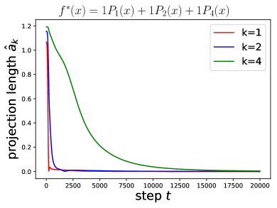
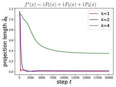
Refer to caption
(a) projection onto training data
Refer to caption
(b) projection onto test data
Refer to caption
(c) projection onto training data
Refer to caption
(d) projection onto test data
Figure 7: Convergence curve for projection length onto vectors (determined by training data) and functions (estimated by test data). We can see that for low-order Gegenbauer polynomials, the network learns the function while for the high-order Gegenbauer polynomial, the network overfits the training data.

References

  • Advani and Saxe (2017) Advani, M. S. and Saxe, A. M. (2017). High-dimensional dynamics of generalization error in neural networks. arXiv preprint arXiv:1710.03667 .
  • Allen-Zhu and Li (2019) Allen-Zhu, Z. and Li, Y. (2019). What can ResNet learn efficiently, going beyond kernels? In Advances in Neural Information Processing Systems.
  • Allen-Zhu et al. (2019) Allen-Zhu, Z., Li, Y. and Song, Z. (2019). A convergence theory for deep learning via over-parameterization. In International Conference on Machine Learning.
  • Andoni et al. (2014) Andoni, A., Panigrahy, R., Valiant, G. and Zhang, L. (2014). Learning polynomials with neural networks. In International Conference on Machine Learning.
  • Arora et al. (2019a) Arora, S., Du, S., Hu, W., Li, Z. and Wang, R. (2019a). Fine-grained analysis of optimization and generalization for overparameterized two-layer neural networks. In International Conference on Machine Learning.
  • Arora et al. (2019b) Arora, S., Du, S. S., Hu, W., Li, Z., Salakhutdinov, R. and Wang, R. (2019b). On exact computation with an infinitely wide neural net. In Advances in Neural Information Processing Systems.
  • Atkinson and Han (2012) Atkinson, K. and Han, W. (2012). Spherical harmonics and approximations on the unit sphere: an introduction, vol. 2044. Springer Science & Business Media.
  • Bach (2017) Bach, F. (2017). Breaking the curse of dimensionality with convex neural networks. Journal of Machine Learning Research 18 1–53.
  • Basri et al. (2020) Basri, R., Galun, M., Geifman, A., Jacobs, D., Kasten, Y. and Kritchman, S. (2020). Frequency bias in neural networks for input of non-uniform density. arXiv preprint arXiv:2003.04560 .
  • Basri et al. (2019) Basri, R., Jacobs, D., Kasten, Y. and Kritchman, S. (2019). The convergence rate of neural networks for learned functions of different frequencies. In Advances in Neural Information Processing Systems.
  • Bietti and Mairal (2019) Bietti, A. and Mairal, J. (2019). On the inductive bias of neural tangent kernels. In Advances in Neural Information Processing Systems.
  • Bordelon et al. (2020) Bordelon, B., Canatar, A. and Pehlevan, C. (2020). Spectrum dependent learning curves in kernel regression and wide neural networks. arXiv preprint arXiv:2002.02561 .
  • Cao and Gu (2019) Cao, Y. and Gu, Q. (2019). Generalization bounds of stochastic gradient descent for wide and deep neural networks. In Advances in Neural Information Processing Systems.
  • Chen and Xu (2020) Chen, L. and Xu, S. (2020). Deep neural tangent kernel and laplace kernel have the same rkhs. arXiv preprint arXiv:2009.10683 .
  • Chizat et al. (2019) Chizat, L., Oyallon, E. and Bach, F. (2019). On lazy training in differentiable programming. In Advances in Neural Information Processing Systems.
  • Cho and Saul (2009) Cho, Y. and Saul, L. K. (2009). Kernel methods for deep learning. In Advances in neural information processing systems.
  • Collobert and Weston (2008) Collobert, R. and Weston, J. (2008). A unified architecture for natural language processing: Deep neural networks with multitask learning. In International Conference on Machine Learning.
  • Du et al. (2019a) Du, S., Lee, J., Li, H., Wang, L. and Zhai, X. (2019a). Gradient descent finds global minima of deep neural networks. In International Conference on Machine Learning.
  • Du et al. (2019b) Du, S. S., Zhai, X., Poczos, B. and Singh, A. (2019b). Gradient descent provably optimizes over-parameterized neural networks. In International Conference on Learning Representations.
  • Frye and Efthimiou (2012) Frye, C. and Efthimiou, C. J. (2012). Spherical harmonics in p dimensions. arXiv preprint arXiv:1205.3548 .
  • Ghorbani et al. (2019) Ghorbani, B., Mei, S., Misiakiewicz, T. and Montanari, A. (2019). Linearized two-layers neural networks in high dimension. arXiv preprint arXiv:1904.12191 .
  • Gunasekar et al. (2018a) Gunasekar, S., Lee, J., Soudry, D. and Srebro, N. (2018a). Characterizing implicit bias in terms of optimization geometry. In International Conference on Machine Learning.
  • Gunasekar et al. (2018b) Gunasekar, S., Lee, J. D., Soudry, D. and Srebro, N. (2018b). Implicit bias of gradient descent on linear convolutional networks. In Advances in Neural Information Processing Systems.
  • Gunasekar et al. (2017) Gunasekar, S., Woodworth, B. E., Bhojanapalli, S., Neyshabur, B. and Srebro, N. (2017). Implicit regularization in matrix factorization. In Advances in Neural Information Processing Systems.
  • He et al. (2015) He, K., Zhang, X., Ren, S. and Sun, J. (2015). Delving deep into rectifiers: Surpassing human-level performance on imagenet classification. In Proceedings of the IEEE international conference on computer vision.
  • He et al. (2016) He, K., Zhang, X., Ren, S. and Sun, J. (2016). Deep residual learning for image recognition. In Proceedings of the IEEE conference on computer vision and pattern recognition.
  • Hinton et al. (2012) Hinton, G., Deng, L., Yu, D., Dahl, G., Mohamed, A.-r., Jaitly, N., Senior, A., Vanhoucke, V., Nguyen, P., Kingsbury, B. et al. (2012). Deep neural networks for acoustic modeling in speech recognition. IEEE Signal processing magazine 29.
  • Jacot et al. (2018) Jacot, A., Gabriel, F. and Hongler, C. (2018). Neural tangent kernel: Convergence and generalization in neural networks. In Advances in neural information processing systems.
  • Jacot et al. (2020) Jacot, A., Şimşek, B., Spadaro, F., Hongler, C. and Gabriel, F. (2020). Implicit regularization of random feature models. arXiv preprint arXiv:2002.08404 .
  • Ji and Telgarsky (2020) Ji, Z. and Telgarsky, M. (2020). Polylogarithmic width suffices for gradient descent to achieve arbitrarily small test error with shallow relu networks. In International Conference on Learning Representations.
  • Lee et al. (2019) Lee, J., Xiao, L., Schoenholz, S. S., Bahri, Y., Sohl-Dickstein, J. and Pennington, J. (2019). Wide neural networks of any depth evolve as linear models under gradient descent. arXiv preprint arXiv:1902.06720 .
  • Li and Liang (2018) Li, Y. and Liang, Y. (2018). Learning overparameterized neural networks via stochastic gradient descent on structured data. In Advances in Neural Information Processing Systems.
  • Li et al. (2018) Li, Y., Ma, T. and Zhang, H. (2018). Algorithmic regularization in over-parameterized matrix sensing and neural networks with quadratic activations. In Conference On Learning Theory.
  • Nacson et al. (2018) Nacson, M. S., Srebro, N. and Soudry, D. (2018). Stochastic gradient descent on separable data: Exact convergence with a fixed learning rate. arXiv preprint arXiv:1806.01796 .
  • Nakkiran et al. (2019) Nakkiran, P., Kaplun, G., Kalimeris, D., Yang, T., Edelman, B. L., Zhang, F. and Barak, B. (2019). Sgd on neural networks learns functions of increasing complexity. In Advances in Neural Information Processing Systems.
  • Rahaman et al. (2019) Rahaman, N., Baratin, A., Arpit, D., Draxler, F., Lin, M., Hamprecht, F., Bengio, Y. and Courville, A. (2019). On the spectral bias of neural networks. In International Conference on Machine Learning.
  • Rosasco et al. (2010) Rosasco, L., Belkin, M. and Vito, E. D. (2010). On learning with integral operators. Journal of Machine Learning Research 11 905–934.
  • Smale and Zhou (2007) Smale, S. and Zhou, D.-X. (2007). Learning theory estimates via integral operators and their approximations. Constructive approximation 26 153–172.
  • Smale and Zhou (2009) Smale, S. and Zhou, D.-X. (2009). Geometry on probability spaces. Constructive Approximation 30 311.
  • Soudry et al. (2018) Soudry, D., Hoffer, E., Nacson, M. S., Gunasekar, S. and Srebro, N. (2018). The implicit bias of gradient descent on separable data. The Journal of Machine Learning Research 19 2822–2878.
  • Su and Yang (2019) Su, L. and Yang, P. (2019). On learning over-parameterized neural networks: A functional approximation prospective. In Advances in Neural Information Processing Systems.
  • Vempala and Wilmes (2019) Vempala, S. and Wilmes, J. (2019). Gradient descent for one-hidden-layer neural networks: Polynomial convergence and sq lower bounds. In Conference on Learning Theory.
  • Vershynin (2010) Vershynin, R. (2010). Introduction to the non-asymptotic analysis of random matrices. arXiv preprint arXiv:1011.3027 .
  • Xu (2018) Xu, Z. J. (2018). Understanding training and generalization in deep learning by fourier analysis. arXiv preprint arXiv:1808.04295 .
  • Xu et al. (2019a) Xu, Z.-Q. J., Zhang, Y., Luo, T., Xiao, Y. and Ma, Z. (2019a). Frequency principle: Fourier analysis sheds light on deep neural networks. arXiv preprint arXiv:1901.06523 .
  • Xu et al. (2019b) Xu, Z.-Q. J., Zhang, Y. and Xiao, Y. (2019b). Training behavior of deep neural network in frequency domain. In International Conference on Neural Information Processing. Springer.
  • Yang and Salman (2019) Yang, G. and Salman, H. (2019). A fine-grained spectral perspective on neural networks. arXiv preprint arXiv:1907.10599 .
  • Zhang et al. (2017) Zhang, C., Bengio, S., Hardt, M., Recht, B. and Vinyals, O. (2017). Understanding deep learning requires rethinking generalization. In International Conference on Learning Representations.
  • Zou et al. (2019) Zou, D., Cao, Y., Zhou, D. and Gu, Q. (2019). Gradient descent optimizes over-parameterized deep ReLU networks. Machine Learning .
  • Zou and Gu (2019) Zou, D. and Gu, Q. (2019). An improved analysis of training over-parameterized deep neural networks. In Advances in Neural Information Processing Systems.