Multi-resolution Graph Neural Network for
Identifying Disease-specific Variations in Brain Connectivity

Abstract

Convolution Neural Network (CNN) recently have been adopted in several neuroimaging studies for diagnosis capturing disease-specific changes in the brain. While many of these methods are designed to work with images in $\mathbb{R}^{n}$ exploiting regular structure of the domain, they are not well-suited to analyze data with irregular structure such as brain connectivity. As there is significant interest in understanding the altered interactions between different brain regions that lead to neuro-disorders, it is important to develop data-driven methods that work with a population of graph data for traditional prediction tasks. In this regime, we propose a novel CNN-based framework with adaptive graph transforms to learn the most disease-relevant connectome feature maps which have the highest discrimination power across diagnostic categories. The backbone of our framework is a multi-resolution representation of the graph matrix which is steered by a set of wavelet-like graph transforms. In this context, our supervised graph learning framework outperforms conventional graph methods that predict diagnostic label only based on the underlying individual graph. Our extensive experiments on two real datasets of functional and structural brain networks show that our multi-resolution framework achieves significantly higher accuracy, precision and recall in predicting diagnostic labels and identifying disease-specific brain connectivities that are associated with brain disorders such as Attention-Deficit/Hyperactivity Disorder (ADHD) and Alzheimer’s Disease (AD).

1 Introduction

Consider a supervised learning setting where a population of graphs $\{G_{i}\}_{i=1}^{N}$ with labels $\{y_{i}\}_{i=1}^{N}$ are given for regression, classification or statistical inference tasks (without node signals). The overall goal here would be to learn a function $f(G_{i})$ that takes a graph $G_{i}$ as an input to accurately predict an outcome $\hat{y}_{i}$ for the graph, i.e., $\hat{y}_{i}=f(G_{i})$. This setting is more challenging than traditional image analyses that operate with data in $\mathbb{R}^{n}$, since individual graphs have arbitrary structure. However, with substantial set of recent data that live in non-Euclidean spaces such as point clouds [21, 33], 3D surface meshes [49, 23], geophysical data [31] and social networks [22], analyzing a population of networks incorporating their inherent topology is emerging in recent scopes of machine learning and computer vision communities. Such a setting is actually quite common in many brain imaging studies that deal with images or image-derived measures in complex domains such as cortical thickness on brain surfaces or brain connectivity, whose main goal is to identify “interpretable” disease specific variation in the brain [3, 44, 47].

Figure 1: Example of multi-resolution representation of brain connectivity in different scales. First figure: original brain network, Second - Fourth: brain network at different scales (i.e., $s_{1}$=$1.2$, $s_{2}$=$1.5$ and $s_{3}$=$1.7$.)

Many neuroimaging studies operate with data from a population of cohort that can be stratified into two or more groups (e.g., diseased vs. control). Given images or image-derived measures acquired from the participants, after registering the images to a common template space (i.e., for voxel-wise correspondence across images), contrasting the different groups at each voxel over the whole brain identifies those regions in the brain that are affected by the variable of interest (e.g., disease or risk factors) [10, 24, 40]. While such regional brain analyses have a rich history of informing spatial variation from various brain diseases, they still suffer from sensitivity issues due to poor correlation between cognitive changes and pathological features from scanned images [17]. Recent studies motivate that characterizing changes in the brain connectivity or network (i.e., graph) that comprise several affected regions yield a better understanding of the brain over traditional spatial analyses [12, 27, 3]. Unfortunately, there exist few frameworks that are capable of performing traditional inference tasks (e.g., classification or regression) on such graph data.

The most critical challenge in the connectivity analysis tasks is that the data are in irregular structure. For regular images in $\mathbb{R}^{n}$, several methods utilize image filtering [41, 15, 18, 20] to increase sensitivity, which take advantage of the regular lattice structure of the domain. For signals defined in non-Euclidean spaces, e.g., a function $f(n)$ that is defined on sampled points $n$ (e.g., graph nodes), recent methods use convolutions on graphs that require special definition of data transformation such as wavelet transform on manifolds [7, 9, 30]. However, when the object of interest is the graph itself and not the signal on data points, the methods described above are not directly applicable. On the other hand, graph kernels embeds graphs directly into a vector space to adopt traditional classification methods that compare local substructures among graphs [14, 34, 37]. Unfortunately, typical kernel techniques are not adaptive and the results may significantly vary depending on the kernel types [42]. Alternative deep learning methods for graph objects such as [48, 38] lose interpretability in space particulary with dense graphs. In the end, there exist very few methods that are capable of adaptively transforming the graph data incorporating the inherent structure of the graphs to increase the sensitivity and maintain location-wise interpretability simultaneously. Especially in the medical imaging studies where the sample-size is small (typically up to only a few hundreds), such a method is highly appreciated when the focus is to detect even subtle changes in brain connectivity yet the data remain extremely high-dimensional.

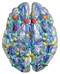
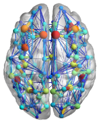
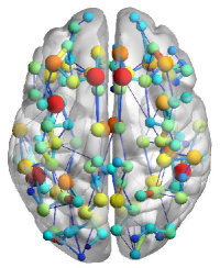
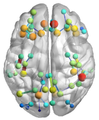
To tackle the issues addressed above, we propose a new convolution neural network (CNN) framework for graph data that derives flexible multi-resolution features (an example shown in Fig. 1) that are highly capable of distinguishing graph from different classes. The core component of our CNN is an adaptive graph transform — we adopt ideas from harmonic analysis on graphs to define a wavelet-like transform that provides novel descriptors at multiple scales for a positive semi-definite (p.s.d.) matrix such as connectivity matrix. The transform yields coefficients by a linear combination of a kernel function (i.e., a band-pass filter) with scaling parameters and orthogonal basis, which shares commonality with traditional continuous wavelet transform that performs band-pass filtering at multiple scales in the frequency space [26]. With a non-linear activation function on the coefficients, we get a multi-resolution feature map of graphs that is trained for graph classification.

In the end, our CNN framework can that not only predict a label (i.e., a disease) of a graph (i.e., a brain network), but also identify which of the individual edges are significantly associated with the prediction. This edge identification is important considering our brain connectivity analysis application, since it will tell us which of the brain connectivities are significantly related to disease-specific variables. Parameterizing a kernel with the notion of scales enables efficient training on the scale parameter and accurate prediction. The main contributions of our work here are, 1) we propose a CNN framework for graphs that can efficiently train and predict labels for a given set of graphs, 2) the proposed algorithm can identify which of the edges in the graphs are significantly affecting the prediction, 3) we provide extensive empirical results on both real functional and structural brain connectivity data (Attention-Deficit/Hyperactivity Disorder (ADHD) dataset and Alzheimer’s Disease (AD) dataset respectively) to validate our framework. Interestingly, the discoveries that we report in our experiments align with other on-going ADHD and AD studies suggesting that our findings are sound, and our framework has potential to be applied to the analyses of various other neurodegenerative diseases.

2 Preliminary: Multi-resolution on Graphs

Our method is built on the philosophy that multi-resolution representation of data driven by convolution will provide a robust means for comparisons of the data from different classes. One of the fundamental approaches to derive the multi-resolution representation is to perform wavelet transform, and we provide a brief review of the wavelet transform and its extension on graphs which will be used to describe our framework in later sections.

2.1 Continuous Wavelet Transform

The concept of a wavelet transform is similar to that of Fourier transform, i.e., both transforms represent a signal as a linear combination of bases and corresponding coefficients. That is, Fourier transform uses $\sin()$ bases to transform an original signal to its Fourier coefficients, and a wavelet transform uses a mother wavelet $\psi$ as the basis, which is a localized and oscillating function. While the $\sin()$ for Fourier transform has infinite support and is localized in frequency space only, the wavelet bases $\psi$ is localized in both time and frequency [35]. A mother wavelet $\psi_{s,a}$ has a scale parameter $s$ and a translation parameter $a$ as $\psi_{s,a}(x)=\frac{1}{s}\psi(\frac{x-a}{s})$ where $s$ controls the dilation and $a$ changes localization of $\psi_{s,a}$. The wavelet transform using $\psi_{s,a}$ as the bases transforms $f(x)$ as

$$\footnotesize W_{f}(s,a)=\langle f,\psi\rangle=\frac{1}{s}\int f(x)\psi^{*}(\frac{x-a}{s})\mathrm{d}x$$ (1)

where $W_{f}(s,a)$ is the wavelet coefficient at scale $s$ and at location $a$, and $\psi^{*}$ is the complex conjugate of $\psi$. Using the coefficients $W_{f}(s,a)$ and the bases $\psi_{s,a}$, we obtain a wavelet expansion of $f(x)$ as a linear combination of them.

Interestingly, if we set $\bar{\psi}_{s}(x)=\frac{1}{s}\psi^{*}(\frac{-x}{s})$, the wavelet transform in (1) can be interpreted as a convolution as

$$W_{f}(s,a) =\frac{1}{s}\int f(x)\psi^{*}(\frac{x-a}{s})\mathrm{d}x$$ (2)

$$=\int\bar{\psi}_{s}(a-x)f(x)\mathrm{d}x$$ (3)

$$=(\bar{\psi}_{s}(x)\star f)(a).$$ (4)

The key in wavelet expansion is that the mother wavelets $\psi_{s}$ at different scales behave as band-pass filters focusing on specific bandwidths in the frequency space. Such behavior offers the multi-resolution representations of the original signal capturing local contexts in various receptive fields.

2.2 Multi-resolution in Non-Euclidean Spaces

Defining a wavelet transform in the Euclidean setting (represented as a regular lattice) was convenient since one can easily design the shape of a mother wavelet for bases. However, in a non-Euclidean setting where the domain is irregular (e.g., a graph), it is difficult to define the key parameters for a mother wavelet such as scale and translation. This is because of the irregularity in the domain, e.g., the distance between vertices and the number of edges in a graph are not uniform, and thus makes it difficult to define a localized mother wavelet at a specific scale. Due to this issue, it has been difficult to adopt the traditional wavelet transform for analyses of data with arbitrary structure.

The breakthrough was to utilize a dual space. The key idea was to define a mother wavelet $\psi_{s}$ in a simple 1D dual space (i.e., an analogue of frequency space) instead of the complex original domain. Recall that the wavelets are band-pass filters in the frequency space. Therefore, if we first construct a localized band-pass filter in the dual domain and transform it back to the original graph space, it would implement a localized mother wavelet on the graph vertices at a specific scale. Such process requires 1) a localized kernel function (i.e., band-pass filter) and 2) orthogonal bases for graphs to define the dual space. Specifically in [13], spectral graph theory was used to define an orthogonal transform.

A graph $G=\{V,E\}$ defined by a vertex set $V$ and an edge set $E$ (with corresponding edge weights $e$) is typically represented as a form of matrix. Given $|V|=N$, an adjacency matrix $A_{N\times N}$ is defined by the connections among the vertices, i.e., the non-zero $a_{i,j}$ in $A$ represents the connection between the $i$-th and $j$-th vertices. A degree matrix $D_{N\times N}$ is a diagonal matrix where the $i$-th diagonal is the sum of edge weights connected to the $i$-th vertex. Subtracting these two matrices defines a graph Laplacian as $\mathcal{L}=D-A$, which is a positive semi-definite (p.s.d.), symmetric and self-adjoint operator. The eigendecomposition of $\mathcal{L}$ yields eigenvalues $\lambda_{l}\geq 0$ and eigenvectors $u_{l}$ where $l=1,\cdots N$, where $u_{l}$ are orthonormal. The $u_{l}$ can be used to define the graph Fourier transform which offers the transform of a signal/measurement on graph nodes/vertices to the frequency domain as

$$\footnotesize\hat{f}(l)=\sum_{n=1}^{N}u^{*}_{l}(n)f(n)~{}\mbox{and}~{}f(n)=\sum_{l=1}^{N}\hat{f}(l)u_{l}(n)$$ (5)

where $\hat{f}(l)$ is the resultant graph Fourier coefficient.

Then, a mother wavelet $\psi_{s}$ can be constructed in the graph Fourier space as a kernel function $k()$ (i.e., localized band-pass filter), and localized on a graph node $n$ by a dirac delta function $\delta_{n}$ through the inverse transform. Using $\langle\delta_{n},u_{l}\rangle=u_{l}^{*}(n)$, the mother wavelet $\psi_{s,n}$ at vertex $n$ at scale $s$ is defined as

$$\footnotesize\psi_{s,n}(m)=\sum_{l=0}^{N-1}k(s\lambda_{l})u_{l}^{*}(n)u_{l}(m)$$ (6)

where $s$ manages dilation of $\psi_{s}$. Using $\psi$ as the bases, the wavelet transform for $f(n)$ on graph nodes is defined as

$$\footnotesize W_{f}(s,n)=\langle f,\psi_{s,n}\rangle=\sum_{l=0}^{N-1}k(s\lambda_{l})\hat{f}(l)u_{l}(n)$$ (7)

which yields wavelet coefficients $W_{f}(s,n)$. Following the reformulation in (4), this operation in (7) can be also viewed as a convolution which will be a key concept for convolution neural network for “graphs” to be introduced later.

3 Multi-resolution Neural Network Framework for Graphs

In the problem posed in this paper, we assume that a set of graphs are provided with a label $y$ assigned for each graph $G$, and each graph is represented as its adjacency matrix form $A$. Here, we consider undirected graph setting whose each positive element $a_{ij}$ denotes the edge weight (i.e., measure of association) between the $i$-th and $j$-th nodes, while zero elements denote no connection between two different nodes. In the following, we introduce a novel transform for graph matrices and use it to design a convolution neural network that predicts labels $\hat{y}$ for graphs $G$.

3.1 Multi-resolution View of Graphs

Consider a graph (e.g., brain network) represented as an adjacency matrix $A$ and its Laplacian $\mathcal{L}$. In (6), the eigenvectors from $\mathcal{L}$ and a kernel function $k()$ were used to define a wavelet basis that is used to derive multi-resolution representation of a function $f(n)$ defined on graph nodes. On the other hand, in our case, we do not have a function $f(n)$ and need a means to define “multi-resolution view for edges”, which will differentiate our method from others previous works [16, 7]. In the following, we choose to continue with graph Laplacian to define a novel graph transform since it is a p.s.d. operator whose eigenvalues are all greater than or equal to 0 and their eigenvector are orthonormal. An outer-product of the eigenvectors will be used as bases for the transform which are still orthonormal.

For a given graph, its corresponding Laplacian representation $\mathcal{L}$ can be decomposed with eigenvalues and eigenvectors in the following way,

$$\footnotesize\mathcal{L}=\overset{N-1}{\underset{l=0}{\sum}}\lambda_{l}u_{l}u_{l}^{T}=U\Lambda U^{T}$$ (8)

where $U=[u_{0},u_{1},\cdots,u_{N-1}]$ and $\Lambda$ is a diagonal matrix whose $l$-th diagonal element is $\lambda_{l}$. Equation (6) suggests defining scaling in a dual space, hence we define a basis as

$$\footnotesize\Psi_{s}=Uk(s\Lambda)U^{T}.$$ (9)

We use this $\Psi_{s}$ to transform the Laplacian $\mathcal{L}$ as

$$\beta_{\mathcal{L}}(s) =\langle\mathcal{L},\Psi_{s}\rangle$$ (10)

$$=(Uk(s\Lambda)U^{T})^{T}U\Lambda U^{T}$$ (11)

$$=Uk(s\Lambda)U^{T}U\Lambda U^{T}$$ (12)

$$=Uk(s\Lambda)\Lambda U^{T}$$ (13)

where $\beta_{\mathcal{L}}(s)$ is the resultant coefficient matrix at scale $s$.

Lemma 1.

(Graph Admissibility Condition) Given a kernel dependent normalization constant $C_{k}=\int_{0}^{\infty}\frac{k(x)^{2}}{x}dx<\infty$, the original graph Laplacian can be perfectly reconstructed via an inverse transformation.

Proof.

Projecting the coefficients $\beta_{\mathcal{L}}(s)$ back to the original domain, we get

$$\frac{1}{C_{k}}\int_{0}^{\infty}\beta_{\mathcal{L}}(s)\Psi_{s}\frac{ds}{s} =\frac{1}{C_{k}}\int_{0}^{\infty}Uk(s\Lambda)\Lambda U^{T}Uk(s\Lambda)U^{T}\frac{ds}{s}$$ (14)

$$=\frac{1}{C_{k}}\int_{0}^{\infty}Uk(s\Lambda)^{2}\Lambda U^{T}\frac{ds}{s}$$ (15)

$$=U[\frac{1}{C_{k}}\int_{0}^{\infty}\frac{k(s\Lambda)^{2}}{s}ds]\Lambda U^{T}$$ (16)

$$=\mathcal{L}$$ (17)

∎

The Lemma above follows the traditional admissibility condition in the continuous wavelet transform [26] integrating multi-resolution wavelet coefficients over the scale $s$, and let us concretely define multi-resolution representation of $\mathcal{L}$ at different scales $s$. Focusing on a specific scale $s$, the representation of $\mathcal{L}_{s}$ then becomes

$$\mathcal{L}_{s} =Uk(s\Lambda)U^{T}((Uk(s\Lambda)U^{T})^{T}U\Lambda U^{T})$$ (18)

$$=Uk(s\Lambda)^{2}\Lambda U^{T}$$

The shapes of $k()$ will determine the shape of wavelet-like basis for the $\mathcal{L}$ and its multi-resolution views. In the later sections, we will use this transform to derive novel representations of a graph which will be used to define a CNN framework for graphs.

3.2 Fast Approximation of Matrix Transform

The transform in 3.1 requires eigendecompostion of a graph Laplacian (or estimating partial set of eigenvectors) which is computationally burdening. It may become a bottleneck when a graph has large number of nodes or there are multiple graphs matrices to transform. This is especially true considering our future applications where we will process multiple graphs to perform classification or regression. We therefore suggest an approximation of the transform in (18) that significantly reduces computation with marginal error inspired by the approach in [13].

Let’s assume $g(\Lambda)=\Lambda k(s\Lambda)^{2}$ and $\tilde{\Lambda}=\frac{2}{\lambda_{max}}\Lambda-I_{N}$ since the largest eigenvalue of a normalized graph Laplacian is bounded at 2. Then, $\tilde{\Lambda}=\Lambda-I_{N}$ and $g(\tilde{\Lambda})=g(\Lambda-I_{N})$. If we expand $g(\Lambda)$ at $I_{N}$, then we get

$$g(\Lambda) =\overset{\infty}{\underset{n=0}{\sum}}\frac{g^{(n)}(I_{N})}{n!}(\Lambda-I_{N})^{n}$$ (19)

$$=\overset{\infty}{\underset{n=0}{\sum}}\frac{g^{(n)}(0_{N})}{n!}\tilde{\Lambda}^{n}.$$

Considering that the elements of $\tilde{\Lambda}$ are in the range [-1, 1], we assume there exists a positive $K$ where if $n>K$, $\tilde{\Lambda}^{n}\rightarrow 0$. Then $g(\Lambda)$ can be further approximated as

$$\footnotesize g(\Lambda)\approx\overset{K}{\underset{n=0}{\sum}}\frac{g^{(n)}(0_{N})}{n!}\tilde{\Lambda}^{n}.$$ (20)

Since $U\Lambda^{m}U^{T}=(U\Lambda U^{T})^{m}$, $\mathcal{L}_{s}$ now can be written as

$$\mathcal{L}_{s} =Ug(\Lambda)U^{T}$$ (21)

$$\approx\overset{K}{\underset{n=0}{\sum}}\frac{g^{(n)}(0_{N})}{n!}U\tilde{\Lambda}^{n}U^{T}$$ (22)

$$\approx\overset{K}{\underset{n=0}{\sum}}\frac{g^{(n)}(0_{N})}{n!}\tilde{\mathcal{L}}^{n}$$ (23)

where $\tilde{\mathcal{L}}=\mathcal{L}-I_{N\times N}$. Using this approximation for the matrix transform, we can make our framework (to be introduced in section 3.3) more efficient and practical to be used in various application domains where the graph size is large or there are a number of graphs to transform.

Figure 2: Overall architecture of our framework. A graph representing matrix is transformed to yield multi-resolution representations, and then fully connected (FC) DNN is applied at the end. Error is backpropagated to train the weights $\mathbf{W^{h}}$ in the FC and adaptively update the scales $\mathbf{s}$ to obtain the optimal representations.

3.3 Multi-resolution Graph Neural Network

Based on the transform introduced in section 3.1, we propose Multi-resolution Graph Neural Network (MGNN) which is a novel convolution neural network framework that utilizes multi-scale representation of graphs (not the signal on the nodes) for classification of graph data. Fig.2 illustrates the overall pipeline of our MGNN, which demonstrates two main components (i.e., convolution and fully connected (FC) layers) in the MGNN.

• Convolution layer: When a graph is inputted to this layer, it returns multi-resolution representations of the graph using the transform in (18) as a tensor, i.e., $|\mathbf{s}|\times N\times N$ where $|\mathbf{s}|$ is the total number of scales. The convolution layer contains $|\mathbf{s}|$ units that represent different resolution of the graph representation.

• FC Layer: this component is a Deep Neural Network (DNN) classifier that takes the multi-resolution features of a graph as an input and predicts its class label. It is a fully connected layer with hidden layers, and connected to $L$ output units (i.e., output layer) where $L$ is the number of available classes. The values computed at each output unit, when normalized, represent the probability of an input belong to a specific class.

The schematic of the MGNN is given in Fig. 2 and it is trained to learn two sets of parameters: 1) scale parameters $\mathbf{s}$ that define the optimal resolutions of a graph for a classification task, and 2) weights $\mathbf{W}^{h}$ associated with the edges between the layers in DNN. One note is that we are not performing pooling which is quite common in many CNN architectures. While it is important to increase efficiency of the algorithm, however without an invertable method for pooling, we want to maintain spatial interpretability especially for neuroimaging applications.

3.4 Training MGNN

Given a training set with $N_{G}$ number of individual graphs $G$ with corresponding labels $y$, the learning process consists of feedforward and backpropagation steps. In the feedforward propagation of MGNN, a graph $G$ is inputted to the neural network as a form of graph Laplacian, and the probability that the $G$ belongs to a particular class is computed at the output layer. Suppose we are given an input graph $G$ with $N$ vertices and a set of initial scales $\mathbf{s}$. First, using the operation in (18), the input $G$ is transformed to $\mathcal{L}_{s}$. Since each $\mathcal{L}_{s}$ is represented as a matrix and when there are $|\mathbf{s}|$ of them, these $\mathcal{L}_{s}$ are combined to consist a tensor as

$$\footnotesize M=\mathcal{L}_{1}\cup\mathcal{L}_{2}\cup\cdots\cup\mathcal{L}_{s}\cup\cdots\cup\mathcal{L}_{|\mathbf{s}|}$$ (24)

which is a feature map $M$ that consists a hidden layer.

In the first layer of DNN module with $T$ hidden units, at each $t$-th hidden unit, the learned features in hidden units are linearly combined with corresponding weights in the first layer of DNN as

$$\footnotesize z_{t}=\overset{|\mathbf{s}|,N,N}{\underset{s,p,q}{\sum}}w^{h}_{t,spq}m_{spq},$$ (25)

where $m_{spq}$ represents a feature in multi-scale graph representation $M$ (i.e., an element at $(p,q)$ in $s$-th scale) and $w^{h}_{t,spq}$ denotes the weight on a connection between a hidden unit $m_{spq}$ to the $t$-th hidden unit of the following layer. In the middle of the FC layer, we used leaky Rectified Linear Unit (leaky-Relu) as an activation function for the $z_{t}$ in each hidden layer in DNN. In the output layer of DNN, a soft-max function was utilized to get the final outcome $o_{l}$ for the $l$-th output unit.

Once the output $o_{l}$ is obtained from the feedforward system above, an error can be computed between the $o_{l}$ and the target value $y_{l}$, i.e., a label with one-hot-encoding for the input graph. In our framework, we used cross-entropy as a measure of classification error as follows:

$$\footnotesize J(\mathbf{s},\mathbf{W}^{h})=-\frac{1}{N_{G}}\overset{N_{G}}{\underset{i=1}{\sum}}\overset{L}{\underset{l=1}{\sum}}\left(y_{il}\ln o_{il}+(1-y_{il})\ln(1-o_{il})\right)$$ (26)

where $N_{G}$ and $L$ are the total number of graphs and the total number of available classes respectively, and $y_{il}$ and $o_{il}$ represents target value and the predicted output at $l$-th output unit of $i$-th input sample respectively. Our framework “adaptively” learns scale parameters $\mathbf{s}$ for novel graph representations and $\mathbf{W}^{h}$ in the FC layer by primarily minimizing the classification error in (26). We backpropagate this error to update these parameters.

In a traditional wavelet transform, the $\mathbf{s}$ is fixed to yield a few theoretical guarantees, however, we will freely explore different aspects of $\mathbf{s}$ to find the optimal resolutions with the smallest loss. Additional regularizations for these parameters will be discussed in a later section.

With the derivatives of error function with respect to connections between different layers in the MGNN, we can further write the gradient of total error function as

$$\footnotesize\nabla J(\mathbf{s},\mathbf{W}^{h})=\frac{1}{N_{G}}\overset{N_{G}}{\underset{i=1}{\sum}}\nabla J_{i}(\mathbf{s},\mathbf{W}^{h})$$ (27)

where $\nabla J_{i}(\mathbf{s},\mathbf{W}^{h})$ is the gradient calculated based on the $i$-th input graph, and this gradient will be used for gradient descent with regularizers described in the following section.

3.4.1 Regularization in MGNN

In order to avoid the overfitting (especially with small sample size) and achieve desirable properties in the learned parameters, we impose the following constraints in our model.

First of all, we assume that not all edges in the graphs are responsible for prediction of class labels, rather only a few of them are highly associated with the variable of interest. This is a natural assumption considering our neuroimaging experiment that will follow later, where changes due to a brain disorder usually do not manifest over the whole brain but sparsely appear in different ROIs in the brain. We therefore impose an $\ell_{1}$-norm constraint to the first layer of $\mathbf{W}^{h}$ which includes the fully connected weights. We expect that this constraint will set many of the elements in the first layer of $\mathbf{W}^{h}$ to zeros and identify the edges that are significantly related the prediction of class labels. Unlike the sparsity property of the first layer of $\mathbf{W}^{h}$, we expect $\mathbf{s}$ to be smooth in a reasonable range so that we obtain a multi-resolution view of the graph instead of getting few extreme views of it, i.e., avoid $\mathbf{s}$ from diverging.

Based on both the multi-resolution graph representation and the constraints mentioned above, a new objective function for a graph classification problem is written as

$$\footnotesize\tilde{J}(\mathbf{s},\mathbf{W}^{h})=J(\mathbf{s},\mathbf{W}^{h})+\frac{\theta_{1}}{2N_{G}}|\mathbf{W}_{1}^{h}|_{1}+\frac{\theta_{2}}{2N_{G}}||\mathbf{s}||_{2}$$ (28)

where $\mathbf{W}_{1}^{h}$ represents the weights of the first layer of DNN module, $\theta_{1}$ and $\theta_{2}$ are the regularization constants for $\ell_{1}$-norm and $\ell_{2}$-norm respectively.

The partial derivative of this new objective function w.r.t. the weight from hidden layer to the output layer becomes

$$\footnotesize\frac{\partial\tilde{J}(\mathbf{s},\mathbf{W}^{h})}{\partial w^{h}_{t,spq}}=\frac{1}{N_{G}}\left(\overset{N_{G}}{\underset{i=1}{\sum}}\frac{\partial J_{i}(\mathbf{s},\mathbf{W}^{h})}{\partial w^{h}_{t,spq}}+\frac{\theta_{1}}{2}\text{sign}(w^{h}_{t,spq})\right),$$ (29)

and similarly, the partial derivative of (28) with respect to $\mathbf{s}$ from the convolution layer to the hidden layer is given by

$$\footnotesize\frac{\partial\tilde{J}(\mathbf{s},\mathbf{W}^{h})}{\partial s}=\frac{1}{N_{G}}\left(\overset{N_{G}}{\underset{i=1}{\sum}}\frac{\partial J_{i}(\mathbf{s},\mathbf{W}^{h})}{\partial s}+\theta_{2}s\right).$$ (30)

With these derivatives, we can now minimize the final objective function (28) and update the parameters of our model using gradient descent with different learning rates $\gamma_{W}$ and $\gamma_{s}$ for $\mathbf{W}^{h}$ and $\mathbf{s}$ respectively.

4 Experiments

In this section, we perform two sets experiments on two real datasets. The ADHD-200 dataset contains resting state functional magnetic resonance images (rs-fMRI) from which we construct functional brain connectivity, whereas we utilize structural brain connectivity from Alzheimer’s Disease Neuroimaging Initive (ADNI) dataset to perform individual analysis for ADHD and AD respectively.

4.1 Datasets

Here, we introduce the following two real independent datasets that are used to validate our MGNN framework.

ADHD-200 dataset. Our experiments were conducted on the public ADHD-200 dataset with data collected from 973 participants in eight different sites [1]. We adopted rs-fMRI data which were registered to Automated Anatomical Labeling (AAL) atlas with 116 regions of interest (ROIs). We used Pearson’s correlation coefficients between different ROIs construct functional brain connectivity for each participant, i.e., a $116\times 116$ adjacency matrix whose rows and columns correspond to ROIs. We had four labels depending on the progression of the ADHD: 1) Typically Developing Children (TDC), 2) ADHD-Combined (ADHD-C), 3) ADHD-Hyperactive/Impulsive (ADHD-H/I) and 4) ADHD-Inattentive (ADHD-I). We removed ADHD-H/I group since it had only 11 samples; taking all the available samples (without any artifact), we ended up with total of $N=756$ samples for our experiment. The demographic of ADHD-200 dataset is given in Table 1.

Table 1: Demographics of ADHD-200 Dataset

Category	TDC	ADHD-C	ADHD-I
# of Subjects	487	159	110
Age (mean, std)	12.2(3.3)	11.2(3.0)	12.0(2.6)
Gender (M/F)	258/229	130/29	85/25

ADNI dataset. ADNI dataset is a public dataset for longitudinal AD study. From the initiative, we obtained Diffusion Tensor Images (DTI), and individual images were processed by tractography pipeline to extract structural brain networks using Destrieux atlas with 148 ROIs. Each brain network is representated as an adjacencey matrix whose elements denote number of neuron fiber tracts connecting two different ROIs. The dataset includes 5 classes: 1) AD, 2) Cognitively Normal (CN), 3) Early Mild Cognitive Impairment (EMCI), 4) Late Mild Cognitive Impairment (LMCI) and 5) Significant Memory Concern (SMC), and the demographics of the ADNI dataset can be found in Table 2. In our experiment, we merged CN and EMCI groups as Pre-clinical AD group and combined LMCI and AD groups as Prodromal AD group to ensure sufficient sample size and compare their differences.

Table 2: Demographics of ADNI dataset

Category	AD	CN	EMCI	LMCI	SMC
# of Subjects	77	109	167	94	59
Age (mean, std)	76.1 (7.05)	73.9 (5.8)	72 (7.48)	72.6 (6.46)	73.6 (4.91)
Gender (M/F)	47/30	57/52	106/61	51/43	21/38

4.2 Experimental Settings

Performance measures. We used 3-fold cross validation (CV) to evaluate our model and baselines with unbiased result. Evaluation measures were accuracy, weighted precision and weighted recall averaged across the CV. We used weighted precision and recall since the class distributions in our datasets were skewed, and these weights were given according to the number of samples in each class.

Parameters. In our experiments, we utilized Adam optimizer for back-propagation. Our kernel function was defined as $k_{s}(x)=sxe^{-sx}$ to ensure that the $k()$ behaves as a band-pass filter (i.e., it achieves 0 at the origin), and the total number of scales to derive multi-resolution representation was $|\mathbf{s}|=5$. Weights were randomly initialized with Xavier initialization and the scales were uniformly selected between $[0,2.5]$. To avoid overfitting, we used dropout of rate $0.2$. $\ell_{1}$-norm was applied on the first layer of DNN with hyper-parameter $0.0001$ to achieve sparsity. $\ell_{2}$-norm was adopted on scales with hyper-parameter $0.001$. The input of DNN module was fixed as 50 and the number of nodes in hidden layers were set to 2000, 128 and 32, respectively. Moreover, LeakyReLU activation function was applied on the output of each hidden layer. Considering the imbalance property in our datasets, we chose to evenly sample training data from each class during the training process. The learning rate of scaling parameters was set to $\gamma_{s}=0.05$, and that of weight parameters was set to $0.01$. For the approximation, the degree of Taylor expansion $K=30$.

Baselines. We used Support Vector Machine with an RBF kernel (RBF-SVM), Logistic regression (LR), graph kernel methods (i.e., Shortest Path (SP) [2] and Weisfeiler-Lehman (WL) [36]) with SVM, and two deep learning frameworks (i.e., graph2vec [29] and Dynamic Graph CNN (DGCNN) [46]) as baselines to compare performances with our MGNN. To deal with the problem of imbalanced dataset, the training dataset was first oversampled using SMOTE [4] before fed into baseline methods. If the method required node features, degree was used as the node feature.

4.3 Functional Brain Connectivity Analysis on ADHD-200

In this section, we analyzed brain connectivity across $116$ ROIs from $N=756$ participants in the ADHD-200 dataset. Each brain connectivity was given as an adjacency matrix in size $116\times 116$ whose individual element was the functional connectivity between two different ROIs in the brain. As described in 4.1, there were three classes which we predicted, and the trained parameters informed which multi-resolution representations were useful and which individual connectivities were responsible for the prediction. As the participants in this dataset are adolescents whose brains are actively developing (high variation), characterizing the differences among these groups was a difficult task.

Table 3: Classification Performances on ADHD-200

Model	Accuracy	wPrecision	wRecall
SVM (RBF)	0.624	0.530	0.624
LR	0.592	0.567	0.592
SP-SVM	0.488	0.495	0.488
WL-SVM	0.516	0.468	0.516
DNN	0.626	0.566	0.626
graph2vec	0.390	0.480	0.390
DGCNN	0.576	0.420	0.576
MGNN (ours)	0.649	0.566	0.649

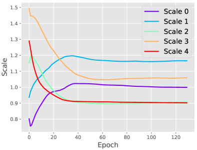
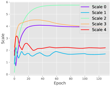
Our results are summarized in Table 3. During our experiments, because the label distribution in the dataset was imbalanced, we have experienced many cases where these algorithms bias towards predicting all testing instances as a single class (i.e., TDC) simply to achieve high accuracy. The parameters for baseline methods were tuned carefully so that such case does not happen, and this effort is shown with high weighted precisions and recalls. MGNN achieved highest accuracy as well as weighted recall compared to all baseline methods except for weighted precision, which was still comparable to the best result with LR. Graph kernel methods with SVM performed even worse than SVM with RBF kernel, it may be because these algorithms are designed to take binary adjacency matrices only instead of weighted ones. Considering that the dataset was imbalanced, it is important that we obtained the highest weighted recall covering even the classes with the less number of samples. DNN was a fully connected neural network that we used; comparing the results from MGNN and DNN, we can see that the multi-resolution representation helped improve the result. Fig.  3 shows the convergence of the scales for multi-resolution, and the one for ADHD experiment is given in the left panel. Interestingly, even if we initially start with $|\mathbf{s}|=5$, some of the scales converged to the same value. They quickly converged — this is important since it would have taken much longer or not even possible to train with small training set if we did not use a parametric kernel.

Figure 3: Convergence of scales w.r.t. epoch during training. Left: ADHD-200 dataset, Right: ADNI dataset.

Figure 4: Top-10 significant brain connectivities that distinguished different groups (i.e., classes). Edge thickness denote average trained edge weight and node size denote its degree. Left panel: results from ADHD analysis, Right panel: results from AD analysis. 1) In the left panel: Top: Sagittal view (left hemisphere), Superior view, Sagittal view (right hemisphere); Bottom: Sagittal view (right hemisphere), Inferior view, Sagittal view (left hemisphere). 2) In the right panel: various views on L: left hemisphere; R: right hemisphere.

Table 4: Top-10 Significant Connectivity from ADHD-200

Row(ROI label [43])	Col(ROI label)
6 (Frontal_Sup_Orb_R)	9 (Frontal_Mid_Orb_L)
7 (Frontal_Mid_L)	24 (Frontal_Sup_Medial_R)
7 (Frontal_Mid_L)	23 (Frontal_Sup_Medial_L)
7 (Frontal_Mid_L)	31 (Cingulum_Ant_L)
7 (Frontal_Mid_L)	32 (Cingulum_Ant_R)
4 (Frontal_Sup_R)	1 (Precentral_L)
107 (Cerebelum_10_L)	108 (Cerebelum_10_R)
70 (Paracentral_Lobule_R)	104 (Cerebelum_8_R)
8 (Frontal_Mid_R)	101 (Cerebelum_7b_L)
64 (SupraMarginal_R)	54 (Occipital_Inf_R)

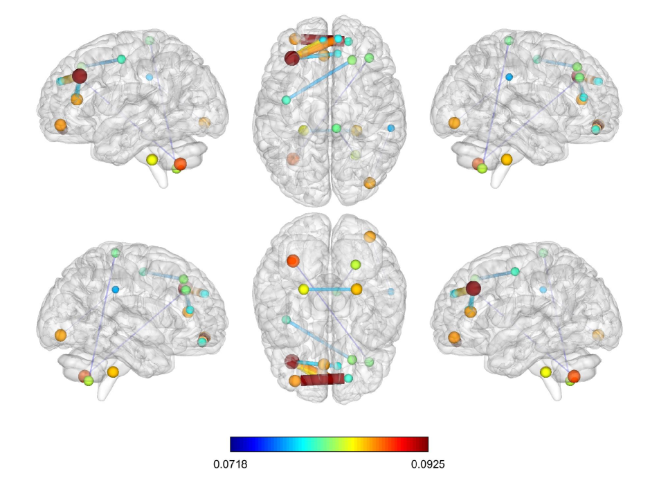
To help clinical interpretation of our findings, we take average of all the trained edge weights that are connected to the trained $\mathcal{L}_{s}$, resize them to the adjacency matrix size, and visualize it as a brain network as in Fig. 4 (left). The top-10 connectivities with the highest average weights are shown for sparsity — these are the most important connectivities in our classification; the thickness of the edges corresponds to the edge weight, and the size of the nodes corresponds to the degree of each ROI. The list of the 10 connections is given in Table 4 that span across 17 ROIs (full ROI names can be found in [43]). We observed that several of them overlapped in Cerebellum [32, 5, 19] and Frontal region [28, 25]; these results are well documented in many ADHD literature.

4.4 Structural Brain Connectivity Analysis on AD

In addition to the functional connectivity analysis on ADHD in section 4.3, we performed structural connectivity analysis on AD. This was a binary classification problem i.e., Pre-clinical AD versus Prodromal AD group to identify differences between the two groups. Instead of classifying 4 groups independently, we chose to perform two group analysis since it benefits increase in sample sizes for each group and let us clearly see the differences between the two groups (i.e., Pre-clinical AD vs. Prodromal AD). We performed 3-fold cross validation multiple times with several settings and reported the best results. The convergence of trained scales can be found in Fig. 3 (right), where we initially start with 5 scales but eventually converge to 4 scales. It suggests that we do not need too many scales to achieve high classification accuracy; but rather only a few optimal scales may be useful for the task.

Table 5: Classification Performances on ADNI Dataset

Model	Accuracy	wPrecision	wRecall
SVM	0.503	0.591	0.503
LR	0.702	0.700	0.702
SP-SVM	0.426	0.535	0.426
WL-SVM	0.456	0.466	0.456
DNN	0.736	0.736	0.736
graph2vec	0.458	0.632	0.458
DGCNN	0.624	0.646	0.624
MGNN (ours)	0.774	0.772	0.774

The classification results are summarized in Table 5. Comparing the different results on accuracy, weighted precision and recall from all baseline models and MGNN, our result outperformed other baseline methods in all evaluation categories. Considering that the decision boundary exists between EMCI and LMCI in the disease spectrum and the differences between them are very subtle, this was not an easy task. As seen in the results with the baseline methods, it was difficult to achieve good performance with brain connectivity classification. Only Neural Network methods (i.e., LR, DNN and DGCNN) yielded reasonable results.

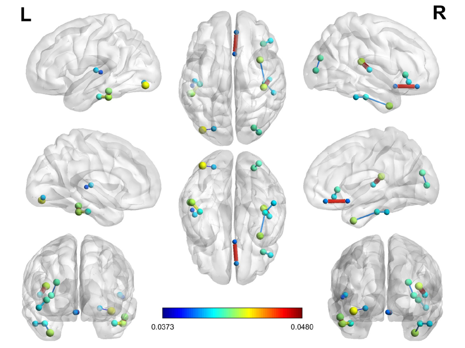
Again, the top-10 connectivities with the largest average of trained weights are visualized in Fig. 4 (right), which are the most significant edges for classifying Pre-clinical and Prodromal AD. The list of these connectivities are given in Table 6 which come from 18 different ROIs (full ROI names can be found in [8]). We observed several temporal regions (i.e., inferior temporal gyrus, inferior temporal sulcus, temporal pole, transverse temporal sulcus) [11, 6] as well as lateral and collateral fissure [39, 45], and many others, which are corroborated by various AD literature.

Table 6: Top-10 Significant Connectivity from ADNI

Row (ROI label [8])	Col (ROI label)
115 (rLat_Fis-post)	107 (rG_temp_sup-G_T_transv)
72 (lS_temporal_inf)	37 (lG_temporal_inf)
106 (rG_subcallosal)	144 (rS_suborbital)
50 (lS_collat_transv_ant)	37 (lG_temporal_inf)
124 (rS_collat_transv_ant)	111 (rG_temporal_inf)
113 (rLat_Fis-ant-Horizont)	87 (rG_front_inf-Orbital)
117 (rPole_temporal)	124 (rS_collat_transv_ant)
131 (rS_oc_middle_and_Lunatus)	132 (rS_oc_sup_and_transversal)
2 (lG_and_S_occipital_inf)	51 (lS_collat_transv_post)
74 (lS_temporal_transverse)	33 (lG_temp_sup-G_T_transv)

5 Conclusion

In this paper, we developed a novel convolution neural network framework that is designed to perform traditional classification tasks with a population of graphs. We first defined a novel graph transform to derive its multi-resolution representations of a graph matrix (not a signal on the nodes), and used them as a means to obtain feature maps that are better suited to perform classification on graphs. Using a parametric kernel, our framework, i.e., MGNN, can train well with relatively small training samples and its effectiveness was validated with extensive experiments on two independent datasets: 1) functional brain connectivity (ADHD-200) and 2) structural brain connectivity (ADNI) datasets. We achieved improved performances over existing baselines, and the results yielded clinically sound results on ADHD and AD that are supported by existing literature. We believe that our MGNN has significant potential to be practically applied to those application domains with graph data where they still suffer from lack of samples.

References

- [1] Pierre Bellec, Carlton Chu, Francois Chouinard-Decorte, et al. The neuro bureau ADHD-200 preprocessed repository. Neuroimage, 144:275–286, 2017.
- [2] Karsten M Borgwardt and Hans-Peter Kriegel. Shortest-path kernels on graphs. In ICDM, pages 8–pp. IEEE, 2005.
- [3] Ed Bullmore and Olaf Sporns. Complex brain networks: graph theoretical analysis of structural and functional systems. Nature Reviews Neuroscience, 10(3):186, 2009.
- [4] Nitesh V Chawla, Kevin W Bowyer, Lawrence O Hall, et al. SMOTE: synthetic minority over-sampling technique. Journal of artificial intelligence research, 16:321–357, 2002.
- [5] Joan M Coffin, Susan Baroody, Kimberly Schneider, and Joshua O’Neill. Impaired cerebellar learning in children with prenatal alcohol exposure: a comparative study of eyeblink conditioning in children with ADHD and dyslexia. Cortex, 41(3):389–398, 2005.
- [6] A Convit, J De Asis, MJ De Leon, CY Tarshish, S De Santi, and H Rusinek. Atrophy of the medial occipitotemporal, inferior, and middle temporal gyri in non-demented elderly predict decline to Alzheimer’s disease. Neurobiology of aging, 21(1):19–26, 2000.
- [7] Michaël Defferrard, Xavier Bresson, and Pierre Vandergheynst. Convolutional neural networks on graphs with fast localized spectral filtering. In NIPS, pages 3844–3852, 2016.
- [8] Christophe Destrieux, Bruce Fischl, Anders Dale, and Eric Halgren. Automatic parcellation of human cortical gyri and sulci using standard anatomical nomenclature. Neuroimage, 53(1):1–15, 2010.
- [9] David K Duvenaud, Dougal Maclaurin, Jorge Iparraguirre, et al. Convolutional networks on graphs for learning molecular fingerprints. In NIPS, pages 2224–2232, 2015.
- [10] Karl J Friston. Statistical parametric mapping. In Neuroscience Databases, pages 237–250. Springer, 2003.
- [11] Clare J Galton, Karalyn Patterson, K Graham, et al. Differing patterns of temporal atrophy in Alzheimer’s disease and semantic dementia. Neurology, 57(2):216–225, 2001.
- [12] Michael D Greicius, Ben Krasnow, Allan L Reiss, et al. Functional connectivity in the resting brain: a network analysis of the default mode hypothesis. Proceedings of the National Academy of Sciences, 100(1):253–258, 2003.
- [13] D.K. Hammond, P. Vandergheynst, and R. Gribonval. Wavelets on graphs via spectral graph theory. Applied and Computational Harmonic Analysis, 30(2):129 – 150, 2011.
- [14] Hisashi Kashima and Akihiro Inokuchi. Kernels for graph classification. In ICDM workshop on active mining, volume 2002, 2002.
- [15] Robert Keys. Cubic convolution interpolation for digital image processing. IEEE transactions on acoustics, speech, and signal processing, 29(6):1153–1160, 1981.
- [16] Thomas N Kipf and Max Welling. Semi-supervised classification with graph convolutional networks. ICLR, 2017.
- [17] David S. Knopman, Clifford R. Jack Jr., et al. Brain injury biomarkers are not dependent on -amyloid in normal elderly. Annals of neurology, 73(4):472–480, 2013.
- [18] Alex Krizhevsky, Ilya Sutskever, and Geoffrey E Hinton. Imagenet classification with deep convolutional neural networks. In NIPS, pages 1097–1105, 2012.
- [19] Aaron Kucyi, Michael J Hove, Joseph Biederman, et al. Disrupted functional connectivity of cerebellar default network areas in attention-deficit/hyperactivity disorder. Human brain mapping, 36(9):3373–3386, 2015.
- [20] Steve Lawrence, C Lee Giles, Ah Chung Tsoi, and Andrew D Back. Face recognition: A convolutional neural-network approach. IEEE Transactions on Neural Networks, 8(1):98–113, 1997.
- [21] Huu M. Le, Thanh-Toan Do, Tuan Hoang, et al. SDRSAC: Semidefinite-based randomized approach for robust point cloud registration without correspondences. In CVPR, June 2019.
- [22] Juzheng Li, Jun Zhu, and Bo Zhang. Discriminative deep random walk for network classification. In Association for Computational Linguistics, pages 1004–1013, 2016.
- [23] Shiwei Li, Zixin Luo, Mingmin Zhen, et al. Cross-atlas convolution for parameterization invariant learning on textured mesh surface. In CVPR, June 2019.
- [24] Michael L Lipton, Erik Gellella, Calvin Lo, et al. Multifocal white matter ultrastructural abnormalities in mild traumatic brain injury with cognitive disability: a voxel-wise analysis of diffusion tensor imaging. Journal of neurotrauma, 25(11):1335–1342, 2008.
- [25] Dawn V Loge, R Dennis Staton, and William W Beatty. Performance of children with ADHD on tests sensitive to frontal lobe dysfunction. Journal of the American Academy of Child & Adolescent Psychiatry, 29(4):540–545, 1990.
- [26] Stéphane Mallat. A wavelet tour of signal processing. Academic press, 1999.
- [27] AR Mclntosh and F Gonzalez-Lima. Structural equation modeling and its application to network analysis in functional brain imaging. Human brain mapping, 2(1-2):2–22, 1994.
- [28] Michael Murias, James M Swanson, and Ramesh Srinivasan. Functional connectivity of frontal cortex in healthy and ADHD children reflected in EEG coherence. Cerebral Cortex, 17(8):1788–1799, 2006.
- [29] Annamalai Narayanan, Mahinthan Chandramohan, Rajasekar Venkatesan, et al. graph2vec: Learning distributed representations of graphs. arXiv preprint arXiv:1707.05005, 2017.
- [30] Mathias Niepert, Mohamed Ahmed, and Konstantin Kutzkov. Learning convolutional neural networks for graphs. In ICML, pages 2014–2023, 2016.
- [31] Nikos G Papadopoulos, Myeong-Jong Yi, Jung-Ho Kim, et al. Geophysical investigation of tumuli by means of surface 3D electrical resistivity tomography. Journal of Applied Geophysics, 70(3):192–205, 2010.
- [32] Thomas Raberger and Heinz Wimmer. On the automaticity/cerebellar deficit hypothesis of dyslexia: balancing and continuous rapid naming in dyslexic and ADHD children. Neuropsychologia, 41(11):1493–1497, 2003.
- [33] Yongming Rao, Jiwen Lu, and Jie Zhou. Spherical fractal convolutional neural networks for point cloud recognition. In CVPR, June 2019.
- [34] Kaspar Riesen and Horst Bunke. Graph classification based on vector space embedding. International Journal of Pattern Recognition and Artificial Intelligence, 23(06):1053–1081, 2009.
- [35] S.Haykin and B. Van Veen. Signals and Systems. Wiley, 2005.
- [36] Nino Shervashidze, Pascal Schweitzer, Erik Jan van Leeuwen, et al. Weisfeiler-lehman graph kernels. Journal of Machine Learning Research, 12(Sep):2539–2561, 2011.
- [37] Nino Shervashidze, SVN Vishwanathan, Tobias Petri, et al. Efficient graphlet kernels for large graph comparison. In Artificial Intelligence and Statistics, pages 488–495, 2009.
- [38] Martin Simonovsky and Nikos Komodakis. Dynamic edge-conditioned filters in convolutional neural networks on graphs. In CVPR, pages 3693–3702, 2017.
- [39] Martin Sjöbeck, Christina Elfgren, Elna-Marie Larsson, et al. Alzheimer’s disease (AD) and executive dysfunction. a case-control study on the significance of frontal white matter changes detected by diffusion tensor imaging (DTI). Archives of gerontology and geriatrics, 50(3):260–266, 2010.
- [40] Stephen M Smith, Mark Jenkinson, Heidi Johansen-Berg, et al. Tract-based spatial statistics: voxelwise analysis of multi-subject diffusion data. Neuroimage, 31(4):1487–1505, 2006.
- [41] Christian Szegedy, Wei Liu, Yangqing Jia, et al. Going deeper with convolutions. In CVPR, pages 1–9, 2015.
- [42] Antoine Jean-Pierre Tixier, Giannis Nikolentzos, Polykarpos Meladianos, and Michalis Vazirgiannis. Graph classification with 2D convolutional neural networks. arXiv preprint arXiv:1708.02218, 2017.
- [43] Nathalie Tzourio-Mazoyer, Brigitte Landeau, Dimitri Papathanassiou, et al. Automated anatomical labeling of activations in SPM using a macroscopic anatomical parcellation of the MNI MRI single-subject brain. Neuroimage, 15(1):273–289, 2002.
- [44] Martijn P Van Den Heuvel and Hilleke E Hulshoff Pol. Exploring the brain network: a review on resting-state fMRI functional connectivity. European neuropsychopharmacology, 20(8):519–534, 2010.
- [45] Jianli Wang, Paul J Eslinger, Richard L Doty, et al. Olfactory deficit detected by fMRI in early Alzheimer’s disease. Brain research, 1357:184–194, 2010.
- [46] Yue Wang, Yongbin Sun, Ziwei Liu, et al. Dynamic graph CNN for learning on point clouds. ACM Transactions on Graphics (TOG), 2019.
- [47] Gagan S Wig, Bradley L Schlaggar, and Steven E Petersen. Concepts and principles in the analysis of brain networks. Annals of the New York Academy of Sciences, 1224(1):126–146, 2011.
- [48] Muhan Zhang, Zhicheng Cui, Marion Neumann, and Yixin Chen. An end-to-end deep learning architecture for graph classification. In AAAI, 2018.
- [49] Hao Zhu, Xinxin Zuo, Sen Wang, Xun Cao, and Ruigang Yang. Detailed human shape estimation from a single image by hierarchical mesh deformation. In CVPR, June 2019.