Periodic mode changing in PSR J1048$-$5832

Abstract

By analysing the data acquired from the Parkes 64-m radio telescope at 1369 MHz, we report on the phase-stationary non-drift amplitude modulation observed in PSR J1048$-$5832. The high-sensitivity observations revealed that the central and trailing components of the pulse profile of this pulsar switch between a strong mode and a weak mode periodically. However, the leading component remains unchanged. Polarization properties of the strong and weak modes are investigated. Considering the similarity to mode changing, we argue that the periodic amplitude modulation in PSR J1048$-$5832 is periodic mode changing. The fluctuation spectral analysis showed that the modulation period is very short ($\sim$2.1 s or $17P_{1}$), where $P_{1}$ is the rotation period of the pulsar. We find that this periodic amplitude modulation is hard to explain by existing models that account for the periodic phenomena in pulsars like subpulse drifting.

1 Introduction

For a given pulsar, even though the individual pulses vary in shape, the mean pulse profile is highly stable with time. However, some pulsars are observed to show emission variability over a wide range of time-scales. It is well known that the Crab pulsar emits occasional high-intensity nanosecond bursts that are called giant pulses (e.g. Hankins et al. 2003). High time resolution observations revealed structure on timescales of a few microseconds in PSR J1136+1551 (Bartel, 1978) which is known as microstructure. The phenomenon of pulse nulling was observed in a lot of pulsars, in which pulsed emission suddenly turns off for several pulse periods and then just as suddenly turns on (Ritchings, 1976; Rankin, 1986; Biggs, 1992; Vivekanand, 1995; Wang et al., 2007; Burke-Spolaor et al., 2012; Gajjar et al., 2012). Mode changing is another kind of emission change where pulsars switch between two or more emission states (e.g. Wang et al. 2007). The time-scale of mode changing and nulling ranges from seconds to hours. Intermittent pulsars switch between on and off emission states with cycles times of days or even years (Kramer et al., 2006; Camilo et al., 2012; Lorimer et al., 2012; Lyne et al., 2017).

Although most of these emission changes are largely considered to be random processes, some changes are reported to show periodicities. Subpulse drifting is the best-known periodic emission variation in which subpulses drift in pulse phase or longitude across a sequence of single pulses (e.g. Weltevrede et al. 2006). The subpulse drifting is a periodic pattern with a characteristic spacing of the subpulses in pulse longitude ($P_{2}$) and pulse number ($P_{3}$). Periodic nulling is another common periodic change. Observations reveal that pulsar nulling is not always a stochastic process (Redman & Rankin, 2009). In some cases, the transitions between the null and the burst states have shown periodicities (Rankin & Wright, 2007, 2008; Herfindal & Rankin, 2007, 2009; Rankin et al., 2013; Basu et al., 2017). In recent years, the periodic non-drift amplitude modulation, which looks very similar to periodic nulling, has been reported in a number of pulsars (Basu et al., 2016; Mitra & Rankin, 2017; Yan et al., 2019). It was reported that the periodic phase-stationary amplitude fluctuation is associated with the presence of a core component in the pulse profile (Basu et al., 2016, 2019a).

PSR J1048$-$5832 (B1046$-$58) is a young (20.3 kyr) pulsar, discovered during a 1.5 GHz Parkes survey of the Galactic plane. It is located in the Carina region at low Galactic latitude and has a spin period of 123.7 ms (Johnston et al., 1992). High-resolution X-ray observations by the Chandra telescope revealed the existence of a faint asymmetric pulsar wind nebula (PWN) surrounding this pulsar. However, no pulsed X-ray emission has been detected from the pulsar (Gonzalez et al., 2006). By analysing the EGRET data, Kaspi et al. (2000) found possible $\gamma$-ray pulsations at $E\ >$ 400 MeV and proposed that PSR J1048$-$5832 was the counterpart of the unidentified $\gamma$-ray source 3EG J1048$-$5840. More recently, $\gamma$-ray pulsations with a double-peaked pulse profile (Abdo et al., 2009) were clearly detected from the pulsar for the first time at $E\ >$ 100 MeV by the Fermi telescope. Radio observations show that the pulsar has a complex profile and the profile varies significantly with frequency (Karastergiou et al., 2005; Johnston et al., 2006). At 1.4 GHz, on average, the leading and central components of the pulse profile exhibit a high degree of linear polarization while the trailing component shows a very low fractional linear polarization (Johnston & Kerr, 2018).

In this paper, we present the results of single-pulse observations at 1.4 GHz for PSR J1048$-$5832 that were made with the Parkes 64-m radio telescope. We aim to explore previously unknown properties of the periodic mode changing in PSR J1048$-$5832. Details of the observations and data processing are given in Section 2. Properties of the observed periodic intensity modulations are presented in Section 3 and the implications of the results are discussed in Section 4. We conclude the paper in Section 5.

2 Observations

The observational data used in our analyses were downloaded from the Parkes Pulsar Data Archive which is publicly available online (Hobbs et al., 2011). The single-pulse observations were made using the Parkes 64-m radio telescope on 2016 April 26 with the the H-OH receiver (Thomas et al., 1990) and the fourth-generation Parkes digital filterbank system PDFB4. See Manchester et al. (2013) for further details of the receiver and backend systems. For the observations reported in this paper, the total bandwidth was 256 MHz centred at 1369 MHz with 512 channels across the band. The data which were sampled every 256 $\mu$s last for 0.5 h and contain 14594 pulses.

The data were first reduced using the DSPSR package (van Straten & Bailes, 2011) to de-disperse and produce single-pulse integrations which preserve information on individual pulses. The pulsar’s rotational ephemeris was taken from the ATNF Pulsar Catalogue V1.60 (Manchester et al., 2005). The single-pulse integrations were recorded using the PSRFITS data format (Hotan et al., 2004) with 256 phase bins per rotation period. Strong narrow-band radio-frequency interference (RFI) and broad-band impulsive RFI in the archive files were removed in affected frequency channels and time sub-integrations, respectively. After RFI mitigation, the single-pulse integrations were processed using the PSRCHIVE pulsar data analysis system (Hotan et al., 2004). The PSRSALSA package (Weltevrede, 2016) which is freely available online, was used to carry out the analysis of fluctuation spectra. Following Yan et al. (2011), we carried out the flux density and polarization calibration for later polarization analysis. The rotation measure (RM) value ($-155~{}\mathrm{rad~{}m^{-2}}$) was obtained from Qiao et al. (1995). Stokes parameters were in accordance with the conventions outlined by van Straten et al. (2010).

3 Results

Single-pulse properties of PSR J1048$-$5832 have not been published before. We present and discuss the single-pulse properties for PSR J1048$-$5832 in this section.

3.1 Nulling or mode changing?

A pulse stack of 400 successive pulses is plotted in Fig. 1. The pulse stack clearly shows periodic modulation for the central and trailing components, while the modulation in the leading component cannot be seen clearly. Pulse energy variations for the same pulse sequence as in Fig. 1 are shown in Fig. 2. The pulse energy distributions for the on-pulse and off-pulse windows for all pulses are presented in Fig. 3. The on-pulse energy was determined for each individual pulse by summing the intensities of the pulse phase bins within the on-pulse region. The on-pulse window was defined as the total longitude range of the integrated pulse profile over which the pulse intensity significantly exceeds the baseline noise (3$\sigma$). The off-pulse energy was calculated in the same way using an off-pulse window of the same duration. In Fig. 3, the off-pulse energy histogram shows a narrow Gaussian distribution peaked about zero, while the broader on-pulse energy distribution shows two Gaussian-like components corresponding to a weak mode and a strong mode.

Fig. 1 gives the impression that the periodic modulation might be periodic nulling. However, Fig. 2 and 3 show that the observed periodic modulation is rather different from pulse nulling in two key aspects. Firstly, the pulse energy effectively drops to zero in real null states, but the pulse energy in Fig. 2 is often larger than zero even during the apparent “null” states. Secondly, real nulls have a similar energy distribution to the off-pulse noise. Hence, a nulling pulsar tends to show a bimodal distribution in the on-pulse energy histogram with two peaks, one at the zero energy and the other at the mean pulse energy. Fig. 3 does show a bimodal on-pulse energy distribution with two peaks, but both peaks are obviously larger than zero. This implies that the mean pulse energy in the apparent “null” states is larger than zero which conflicts with real null pulses. The polarization analysis in subsection  3.4 shows that the central and trailing components of the pulse profile switch between a stable strong mode and a stable weak mode periodically while the leading component remains unaffected by the modulation. This is very similar to mode changing. Therefore, in this paper, we argue that the observed periodic modulation in PSR J1048$-$5832 is in fact periodic mode changing rather than periodic pulse nulling.

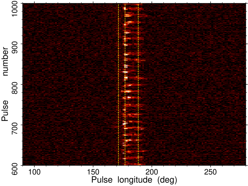
Figure 1: A single-pulse stack of 400 successive pulses. The three vertical dashed lines show the longitudes of the leading, central and trailing pulse peaks of the mean pulse profile respectively.

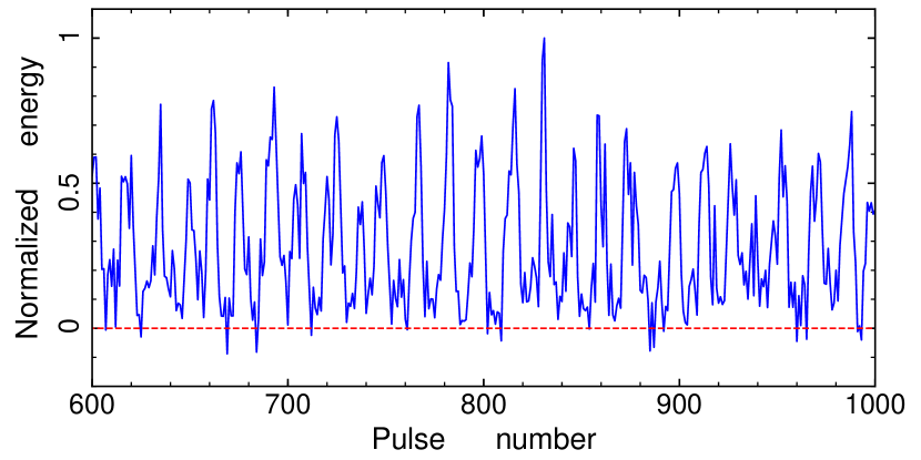
Figure 2: Pulse energy variations for the pulse sequence shown in Fig. 1.

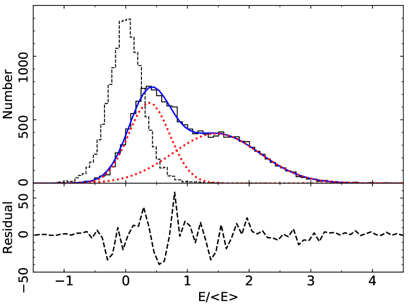
Figure 3: Pulse energy distributions for the on-pulse (solid histogram) and off-pulse (dashed histogram) regions. The energies are normalised by the mean on-pulse energy. The blue solid line represents the fitting for the on-pulse energy distribution based on the combination of two Gaussian components (red dotted lines). The lower panel shows the fit residuals.

3.2 Fluctuation spectra

Fig. 1 clearly shows an apparently periodic modulation for the central and trailing components. To investigate the periodicity further, we plotted the longitude-resolved modulation index, the longitude-resolved fluctuation spectrum (LRFS, Backer, 1970) and the two-dimensional fluctuation spectrum (2DFS, Edwards & Stappers, 2002) in Fig. 4. The longitude-resolved modulation index $m_{i}$ (points with error bars in the top panel) is a measure of the amount of intensity variability from pulse to pulse for each pulse longitude, defined by

$$m_{i}=\frac{\sigma_{i}}{\mu_{i}},$$ (1)

where $\mu_{i}$ and $\sigma_{i}$ are the average intensity and standard deviation at phase bin $i$ respectively. The LRFS and 2DFS are effective for analysing subpulse modulation. The LRFS can be used to determine which pulse phase bins present periodic subpulse modulation and with which periodicities, while the 2DFS can be used to identify whether the subpulse drifts in pulse longitude from pulse to pulse. The vertical frequency axis of both the LRFS and 2DFS corresponds to $P_{1}/P_{3}$, where $P_{1}$ is the rotation period of the pulsar and $P_{3}$ represents the periodicity of intensity modulation that can be seen in the single-pulse stack (Fig. 1). The horizontal frequency axis of the 2DFS corresponds to $P_{1}/P_{2}$, where $P_{2}$ represents the characteristic horizontal time separation between drifting bands. For more details regarding the techniques of analysis, please refer to Weltevrede et al. (2006).

From Fig. 4, we can see that the leading component and the saddle region between the central and trailing components have the lowest modulation index. However, the average intensity is much higher for the saddle region. From the definition of modulation index (Equation (1)), there is just a very weak modulation for the leading component. The side panel of the LRFS shows a clear spectral peak occurring between 0.0571 and 0.0581 cycles per period (cpp). This spectral feature corresponds to the characteristic $P_{3}$ of $17.4\pm 0.2\;P_{1}$ for the periodic modulation. In the LRFS, the spectral feature is stronger in the central and trailing components, implying that most of the periodic modulation power is associated with these components. In addition to the well-defined spectral feature, there are white noise components which are clearly seen as two vertical darker bands in the LRFS around the leading edge of the central component and the peak of the trailing component respectively. These indicate non-periodic stochastic fluctuations at these pulse longitudes. The 2DFS is basically symmetric about the vertical axis, so subpulses in successive pulses do not drift on average to later or earlier pulse longitudes.

Furthermore, to make it clear whether there is any low level periodic behavior in the leading component hidden by the high signal to noise variations in the other two components, we plotted the 2DFS only for the leading component in Fig. 5. A red-noise-like component is strongest below $P_{1}/P_{3}$ = 0.005 cpp, corresponding to fluctuation on a timescale of 200 pulse periods and above. There is no visible periodic feature in the leading component around $P_{3}\simeq 17.4P_{1}$.

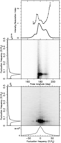
Figure 4: Fluctuation analysis for PSR J1048$-$5832. The mean pulse profile (solid line) and longitude-resolved modulation index (points with error bars) are shown in the top panel. The LRFS with a side panel showing the horizontally integrated power is given below this panel. The 2DFS with side panels showing horizontally (left) and vertically (bottom) integrated power is plotted below the LRFS.

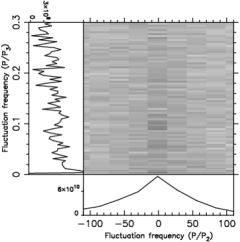
Figure 5: The 2DFS for the leading component. See Fig. 4 for further details.

3.3 Mode separation

To obtain the relative abundances of the strong and weak modes, modeling of the on-pulse energy histogram was carried out by fitting two Gaussian functions. We used the curve_fit function of the scipy python module, which uses non-linear least squares to fit a function to data, to fit the sum of two Gaussian functions to the histogram and the parameters of the fitted Gaussians are listed in Table 1. The results are presented in Fig. 3 which shows that the two modes overlap with no clear boundary between them. Then the relative abundances of each mode can be simply obtained by calculating the area under each Gaussian function. The results show that this pulsar spends 43% in the weak mode and 57% in the strong mode.

Table 1: Parameters of fitted Gaussian functions.

Mode	Amplitude	Mean	Standard Deviation
Weak mode	634	0.38	0.33
Strong mode	391	1.47	0.71

Separation of the strong and weak modes is required for more detailed investigation. However, the above mentioned Gaussian fitting method cannot distinguish pulses in the overlapped area of the two Gaussian functions. Following Bhattacharyya et al. (2010), we identified the two modes by comparing the on-pulse energy of individual pulses with the system noise level. The uncertainty in the on-pulse energy $\sigma_{\rm on}$ is given by $\sqrt{N_{\rm on}}\sigma_{\rm off}$ , where $N_{\rm on}$ is the number of on-pulse phase bins, estimated from the mean pulse profile, and $\sigma_{\rm off}$ is the rms of the off-pulse region for individual pulses. Pulses with on-pulse energy smaller than $3\sigma_{\rm on}$ were classified as weak-mode pulses and the others were classified as strong-mode pulses. Fig. 6 shows the results of the state separation for the same pulse energy sequence as Fig. 2. By performing the state separation in this way for all data, we found that 65% of the time for PSR J1048$-$5832 was in the strong mode and 35% was in the weak mode. There are some differences in values of the relative abundances of the strong and weak modes obtained using two methods. This is because neither method can completely separate the two modes. In the absence of perfect mode separation, we acknowledge that there is always a possibility of mode mixing which may affect the conclusions in our subsequent analysis for profile shape evolution, polarization, etc.

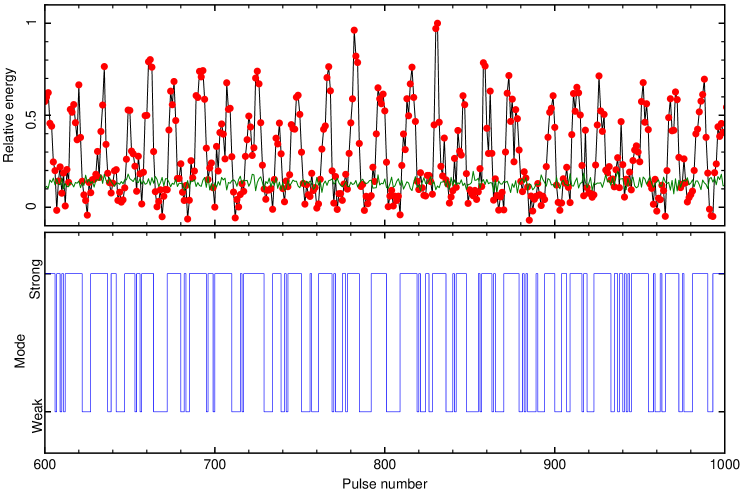
Figure 6: The same pulse energy sequence as Fig. 2 (upper panel) with the corresponding identified strong/weak mode (lower panel). In the upper panel, a red dot is the on-pulse energy of a given pulse and the green line represents the three times level of the uncertainty in the pulse energy estimate for individual pulses (see text for details). Pulses for which pulse energy below the green line were tagged as weak-mode pulses and pulses above the green line were tagged as strong-mode pulses.

3.4 Polarization

To compare the weak mode and the strong mode further, we analysed the polarization properties for both modes. We show mode-separated polarization profiles in Fig. 7, and Table 2 gives a summary of the flux density and polarization parameters for different modes. Columns (2) to (4) give the peak flux density for the leading ($S_{\rm pk,leading}$), central ($S_{\rm pk,central}$) and trailing ($S_{\rm pk,trailing}$) components respectively. The next column gives the mean flux density $S$. Pulse width at 50 per cent of the peak flux density $W_{50}$ is given next. The next three columns give the fractional linear polarization $\langle L\rangle/S$, the fractional net circular polarization $\langle V\rangle/S$ and the fractional absolute circular polarization $\langle|V|\rangle/S$, where $\langle\rangle$ means an average across the pulse profile. Polarization properties of each profile component in different modes are given in Table 3. We defined the outer boundaries of the leading and trailing components as the first point and the last point where the pulse intensity significantly exceeds the baseline noise (3$\sigma$) respectively, while the inner boundaries were defined as the points of minimal intensity between adjacent components. The width of a given component was measured as the longitude range between its two boundaries. The second column $\phi_{\mathrm{pk}}$ in each mode in Table 3 represents the longitudinal position of component peaks.

In Fig. 7, the polarization profile for the average profile in the left panel is in good agreement with previously published results (Rookyard et al., 2015; Johnston & Kerr, 2018). The pulse profile has multiple overlapping features. The leading and the central parts of the profile have very high fractional linear polarization, whereas the trailing part of the profile is essentially unpolarized. Except for the central component, circular polarization is quite weak. The position angle (PA) swing is S-shaped through the profile and relatively shallow in the leading and trailing components. This means that neither the leading component nor the trailing component can be core emission. Based on a rotating vector model (RVM, Radhakrishnan & Cooke, 1969) fit to the PA variations and other constraints, Rookyard et al. (2015) gave an estimate of the impact parameter (the closest approach of the line of sight to the magnetic axis) $0\degr<\beta<7\aas@@fstack{\circ}5$ and suggested that magnetic axis was relatively aligned with the rotation axis, with an inclination angle $\alpha<50\degr$. With the constraints on $\alpha$ and $\beta$ reported by Rookyard et al. (2015), we carried out an RVM fit to the PA swing for the average profile using the ppolFit program of PSRSALSA. The S-shaped solid curve in the top left panel in Fig. 7 shows the best fit to the PA with $\alpha=4\aas@@fstack{\circ}1$ and $\beta=0\aas@@fstack{\circ}7$. The best fit has a reduced $\chi^{2}=5.4$ . The impact parameter $\beta$ is quite small implying that the central component is probably the core component. The strong mode has very similar polarization properties, which just shows stronger central and trailing components. However, the weak mode shows a very different polarization profile. The leading component is the weakest in the strong mode whereas the trailing component is the weakest in the weak mode. The central component in the weak mode is also relatively weak. The central component remains nearly 100 per cent linearly polarized in different modes. The trailing component is essentially unpolarized in the strong mode, while it becomes 100 per cent linearly polarized in the weak mode. The fractional circular polarization in the weak mode is relatively high with a sense reversal between the leading and central components. Both the PA swing and the overall pulse width are identical for the two modes and such behavior has also been seen in PSRs J1822$-$2256 (Basu & Mitra, 2018) and J2006$-$0807 (Basu et al., 2019b), which suggests that the emission of the two modes comes from the same general emission region. Additionally, we compare total intensity of the two modes in Fig. 8. This figure clearly shows that the total intensity of the leading component remains unchanged in the two modes. That is, the main difference between the two modes lies in the central and trailing components. This implies that the observed periodic mode changing arises from variations in the central and trailing components while the leading component is not affected by the mode changing.

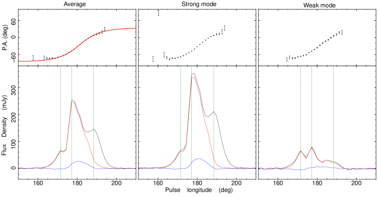
Figure 7: Polarization profiles for the average of all pulses (left), the strong-mode pulses (middle), and the weak-mode pulses (right). The lower panels show the pulse profiles for total intensity (black line), linearly polarized intensity (red line), and circularly polarized intensity (blue line). The upper panels give the position angles of the linearly polarized emission. The three vertical lines show the longitudes of the leading, central and trailing pulse peaks of the mean pulse profile for all pulses respectively. The S-shaped solid line in the top left panel represents the best fit of the PA swing.

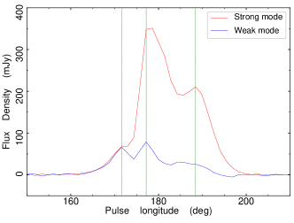
Figure 8: The comparison of the average profile for pulses in the strong mode and the weak mode. The three vertical lines show the longitudes of the leading, central and trailing pulse peaks of the mean pulse profile for all pulses respectively.

Table 2: Flux density and polarization parameters for the strong and weak modes.

Mode	$S_{\rm pk,leading}$	$S_{\rm pk,central}$	$S_{\rm pk,trailing}$	$S$	$W_{50}$	$\left.\left\langle{L}\right\rangle\middle/S\right.$	$\left.\left\langle{V}\right\rangle\middle/S\right.$	$\left.\left\langle\left|{V}\right|\right\rangle\middle/S\right.$
	(mJy)	(mJy)	(mJy)	(mJy)	($\degr$)	(%)	(%)	(%)
Average	66	253	145	10.1	14.9	74.6	6.2	7.2
Strong mode	67	348	211	16.1	15.1	69.3	5.8	6.7
Weak mode	66	79	25	3.9	10.4	95.6	2.0	10.8

Table 3: Polarization parameters of each pulse profile component for the strong and weak modes.

Component	Strong mode						Weak mode
	Width	$\phi_{\mathrm{pk}}$	$\left.\left\langle{L}\right\rangle\middle/S\right.$	$\left.\left\langle{V}\right\rangle\middle/S\right.$	$\left.\left\langle\left|{V}\right|\right\rangle\middle/S\right.$		Width	$\phi_{\mathrm{pk}}$	$\left.\left\langle{L}\right\rangle\middle/S\right.$	$\left.\left\langle{V}\right\rangle\middle/S\right.$	$\left.\left\langle\left|{V}\right|\right\rangle\middle/S\right.$
	($\degr$)	($\degr$)	(%)	(%)	(%)		($\degr$)	($\degr$)	(%)	(%)	(%)
Leading component	9.9	172.2	91.9	$-2.0$	3.3		11.3	172.2	92.3	$-9.7$	9.7
Central component	12.7	179.3	91.8	9.1	9.1		8.5	177.9	100.0	8.3	9.0
Trailing component	14.1	189.2	24.2	1.7	3.1		16.9	186.4	90.0	9.0	17.9

4 Discussion

More and more periodic amplitude fluctuation phenomena have been observed in radio pulsar emission. Basu et al. (2016) carried out a detailed fluctuation spectral analysis for 123 pulsars that were observed at 333 and/or 618 MHz by the GMRT telescope. They revealed periodic features in 57 pulsars, including 29 pulsars where the periodic features show no phase variation but periodic amplitude fluctuation. They discovered the dependence of the drifting phenomenon on the spin-down luminosity $\dot{E}$. In those 57 pulsars, subpulse drifting is only seen in pulsars with $\dot{E}<5\times$10${}^{32}\ {\rm erg\,s^{-1}}$ and the drifting periodicity $P_{3}$ is anticorrelated with $\dot{E}$, whereas other pulsars with $\dot{E}>5\times$10${}^{32}\ {\rm erg\,s^{-1}}$ all showed phase-stationary non-drift amplitude modulation. Basu et al. (2019a) verified this dependence using a larger sample of drifting measurements. PSR J1048$-$5832 has an $\dot{E}=2\times$10${}^{36}\ {\rm erg\,s^{-1}}$ (Wang et al., 2000), and thus lies in the non-drift amplitude modulation group.

Based on empirical classification for the pulse profiles of radio pulsars, Rankin (1983, 1990, 1993) suggested a core/cone model for the radio emission beam. In this model, the emission beam consists of multiple nested cones around a central core component. Different numbers of pulse components result from different line of sight (LOS) trajectories across the beam. Basu et al. (2016) found that the periodic non-drift amplitude modulation was usually found in pulsars with core components. By analysing phase variations corresponding to the drifting features, Basu et al. (2019a) proposed a classification scheme for the phenomenon of subpulse drifting, and they argued that the drifting classification was associated with the profile types and LOS geometry. The periodic non-drift amplitude modulation corresponds to an LOS close to the beam center that sweeps across both the core and the cone regions. In this case, pulsars show the presence of a central core component in their profiles where the drifting is absent, while the conal components show relatively smaller phase variations. However, PSR J1048$-$5832 does not match the pattern. Polarization profiles suggest that the leading and trailing components may be conal components (see Fig. 7) and the small impact parameter implies that the central component is probably the core component. But the fluctuation spectra shown in Fig. 4 show that the central component and the trailing conal component exhibit strong periodic modulation, while the leading conal component is unmodulated, which is not consistent with the simple LOS geometry model of Basu et al. (2019a).

Periodic nulling has been reported in some pulsars (Herfindal & Rankin, 2007, 2009; Rankin & Wright, 2008; Rankin et al., 2013; Gajjar et al., 2014; Gajjar et al., 2017; Basu et al., 2017; Basu & Mitra, 2018; Basu et al., 2019b; Basu & Mitra, 2019). Observed periodicities in the amplitude modulation of some components of some pulsars are very similar to periodic nulling, and therefore Basu et al. (2017) suggested that they have a common origin. This supports the argument of Wang et al. (2007) that nulling and mode changing are different manifestations of the same phenomenon. Here we therefore suggest that periodic nulling is the extreme form of periodic mode changing and that the two phenomena are just different categories of the same physical phenomenon. Some investigators argue that periodic nulling can be explained by the rotating subbeam carousel model (Herfindal & Rankin, 2007), in which the evenly spaced conal subbeams rotate around a central core component. Empty LOS cuts or extinguished subbeams can repeat after certain spin periods of the pulsar, thus giving rise to periodic nulling. However, Basu et al. (2017) found that the missing LOS model did not adequately explain the periodic nulling observed in pulsars with core components. Additionally, (Gajjar et al., 2017) found that the missing LOS model is probably not applicable to the quasi-periodic changes between the null and burst states seen in PSR J1741$-$0840. For the periodic amplitude modulation of PSR J1048$-5832$ reported in this paper, the probable central core component and the trailing conal component switch between a strong mode and a weak mode periodically. The weak mode shows relatively weak emission, but not complete nulls. This does not fit very well with the missing LOS model. Furthermore, the leading conal component is not modulated, which cannot be explained with the rotating subbeam carousel model. The polarization difference of the trailing component in different modes is also not readily explained with the carousel model.

Mitra & Rankin (2017) reported a similar periodic non-drift modulation in PSR B1946+35, in which the highly periodic amplitude modulation was seen in the core component. This could also not be explained using the carousel model and was considered as an entirely new phenomenon. In a recent work by Basu & Mitra (2019), the periodic amplitude modulation has also been seen in the core single pulsar PSR J0826+2637. A periodic phase-stationary intensity modulation occurring in the interpulse and the main pulse was observed in PSR J1825$-$0935 (Fowler & Wright, 1982; Gil et al., 1994; Backus et al., 2010; Latham et al., 2012; Hermsen et al., 2017; Yan et al., 2019). Similar to PSR J1048$-5832$, the main pulse of PSR J1825$-$0935 is partially modulated with an unmodulated trailing component. The periodic amplitude modulation in PSRs J1048$-$58321, B1946+35, J0826+2637 and J1825$-$0935 is probably regular switching between two emission states, i.e., mode changing. We argue that this amplitude modulation is periodic mode changing which results from similarly periodic fluctuations in the magnetospheric field currents that are not directly related to subpulse drifting.

5 Conclusions

We report here a periodic phase-stationary non-drift amplitude modulation observed in PSR J1048$-$5832 using the Parkes 64-m radio telescope. As argued above, the amplitude modulation cannot be reconciled with the subpulse drifting phenomenon in any existing geometrical context. It seems to require emission-state changing in the magnetospheric field currents with the same periodicity. This is similar to the mode changing phenomenon, though the time-scale of mode changing is usually longer. Therefore we suggest the periodic amplitude modulation in PSR J1048$-$5832 is periodic mode changing. Discovering and observing more samples with this amplitude modulation using large radio telescopes such as FAST will throw more light on the nature of this phenomenon.

References

- (1)
- Abdo et al. (2009) Abdo A. A., et al., 2009, ApJ, 706, 1331
- Backer (1970) Backer D. C., 1970, Nature, 227, 692
- Backus et al. (2010) Backus I., Mitra D., Rankin J. M., 2010, MNRAS, 404, 30
- Bartel (1978) Bartel N., 1978, A&A, 62, 393
- Basu & Mitra (2018) Basu R., Mitra D., 2018, MNRAS, 476, 1345
- Basu & Mitra (2019) Basu R., Mitra D., 2019, MNRAS, 487, 4536
- Basu et al. (2016) Basu R., Mitra D., Melikidze G. I., Maciesiak K., Skrzypczak A., Szary A., 2016, ApJ, 833, 29
- Basu et al. (2017) Basu R., Mitra D., Melikidze G. I., 2017, ApJ, 846, 109
- Basu et al. (2019a) Basu R., Mitra D., Melikidze G. I., Skrzypczak A., 2019a, MNRAS, 482, 3757
- Basu et al. (2019b) Basu R., Paul A., Mitra D., 2019b, MNRAS, 486, 5216
- Bhattacharyya et al. (2010) Bhattacharyya B., Gupta Y., Gil J., 2010, MNRAS, 408, 407
- Biggs (1992) Biggs J. D., 1992, ApJ, 394, 574
- Burke-Spolaor et al. (2012) Burke-Spolaor S., et al., 2012, MNRAS, 423, 1351
- Camilo et al. (2012) Camilo F., Ransom S. M., Chatterjee S., Johnston S., Demorest P., 2012, ApJ, 746, 63
- Edwards & Stappers (2002) Edwards R. T., Stappers B. W., 2002, A&A, 393, 733
- Fowler & Wright (1982) Fowler L. A., Wright G. A. E., 1982, A&A, 109, 279
- Gajjar et al. (2012) Gajjar V., Joshi B. C., Kramer M., 2012, MNRAS, 424, 1197
- Gajjar et al. (2014) Gajjar V., Joshi B. C., Wright G., 2014, MNRAS, 439, 221
- Gajjar et al. (2017) Gajjar V., Yuan J. P., Yuen R., Wen Z. G., Liu Z. Y., Wang N., 2017, ApJ, 850, 173
- Gil et al. (1994) Gil J. A., et al., 1994, A&A, 282, 45
- Gonzalez et al. (2006) Gonzalez M. E., Kaspi V. M., Pivovaroff M. J., Gaensler B. M., 2006, ApJ, 652, 569
- Hankins et al. (2003) Hankins T. H., Kern J. S., Weatherall J. C., Eilek J. A., 2003, Nature, 422
- Herfindal & Rankin (2007) Herfindal J. L., Rankin J. M., 2007, MNRAS, 380, 430
- Herfindal & Rankin (2009) Herfindal J. L., Rankin J. M., 2009, MNRAS, 393, 1391
- Hermsen et al. (2017) Hermsen W., et al., 2017, MNRAS, 466, 1688
- Hobbs et al. (2011) Hobbs G., et al., 2011, PASA, 28, 202
- Hotan et al. (2004) Hotan A. W., van Straten W., Manchester R. N., 2004, PASA, 21, 302
- Johnston & Kerr (2018) Johnston S., Kerr M., 2018, MNRAS, 474, 4629
- Johnston et al. (1992) Johnston S., Lyne A. G., Manchester R. N., Kniffen D. A., D’Amico N., Lim J., Ashworth M., 1992, MNRAS, 255, 401
- Johnston et al. (2006) Johnston S., Karastergiou A., Willett K., 2006, MNRAS, 369, 1916
- Karastergiou et al. (2005) Karastergiou A., Johnston S., Manchester R. N., 2005, MNRAS, 359, 481
- Kaspi et al. (2000) Kaspi V. M., Lackey J. R., Mattox J., Manchester R. N., Bailes M., Pace R., 2000, ApJ, 528, 445
- Kramer et al. (2006) Kramer M., Lyne A. G., O’Brien J. T., Jordan C. A., Lorimer D. R., 2006, Science, 312, 549
- Latham et al. (2012) Latham C., Mitra D., Rankin J., 2012, MNRAS, 427, 180
- Lorimer et al. (2012) Lorimer D. R., Lyne A. G., McLaughlin M. A., Kramer M., Pavlov G. G., Chang C., 2012, ApJ, 758, 141
- Lyne et al. (2017) Lyne A. G., et al., 2017, ApJ, 834, 72
- Manchester et al. (2005) Manchester R. N., Hobbs G. B., Teoh A., Hobbs M., 2005, AJ, 129, 1993
- Manchester et al. (2013) Manchester R. N., et al., 2013, PASA, 30, e017
- Mitra & Rankin (2017) Mitra D., Rankin J., 2017, MNRAS, 468, 4601
- Qiao et al. (1995) Qiao G. J., Manchester R. N., Lyne A. G., Gould D. M., 1995, MNRAS, 274, 572
- Radhakrishnan & Cooke (1969) Radhakrishnan V., Cooke D. J., 1969, Astrophys. Lett., 3, 225
- Rankin (1983) Rankin J. M., 1983, ApJ, 274, 333
- Rankin (1986) Rankin J. M., 1986, ApJ, 301, 901
- Rankin (1990) Rankin J. M., 1990, ApJ, 352, 247
- Rankin (1993) Rankin J. M., 1993, ApJ, 405, 285
- Rankin & Wright (2007) Rankin J. M., Wright G. A. E., 2007, MNRAS, 379, 507
- Rankin & Wright (2008) Rankin J. M., Wright G. A. E., 2008, MNRAS, 385, 1923
- Rankin et al. (2013) Rankin J. M., Wright G. A. E., Brown A. M., 2013, MNRAS, 433, 445
- Redman & Rankin (2009) Redman S. L., Rankin J. M., 2009, MNRAS, 395, 1529
- Ritchings (1976) Ritchings R. T., 1976, MNRAS, 176, 249
- Rookyard et al. (2015) Rookyard S. C., Weltevrede P., Johnston S., 2015, MNRAS, 446, 3367
- Thomas et al. (1990) Thomas B. M., Greene K. J., James G. L., 1990, I.E.E.E. Trans. Ant. Propag., 38, 1898
- van Straten & Bailes (2011) van Straten W., Bailes M., 2011, PASA, 28, 1
- van Straten et al. (2010) van Straten W., Manchester R. N., Johnston S., Reynolds J. E., 2010, PASA, 27, 104
- Vivekanand (1995) Vivekanand M., 1995, MNRAS, 274, 785
- Wang et al. (2000) Wang N., Manchester R. N., Pace R., Bailes M., Kaspi V. M., Stappers B. W., Lyne A. G., 2000, MNRAS, 317, 843
- Wang et al. (2007) Wang N., Manchester R. N., Johnston S., 2007, MNRAS, 377, 1383
- Weltevrede (2016) Weltevrede P., 2016, A&A, 590, A109
- Weltevrede et al. (2006) Weltevrede P., Edwards R. T., Stappers B. W., 2006, A&A, 445, 243
- Yan et al. (2011) Yan W. M., et al., 2011, MNRAS, 414, 2087
- Yan et al. (2019) Yan W. M., Manchester R. N., Wang N., Yuan J. P., Wen Z. G., Lee K. J., 2019, MNRAS, 485, 3241