Computing the Small-Scale Galaxy Power Spectrum and Bispectrum in Configuration-Space

Oliver H. E. Philcox1,2 and Daniel J. Eisenstein2
1Department of Astrophysical Sciences, Princeton University, Princeton, NJ 08544, USA
2Center for Astrophysics | Harvard & Smithsonian, 60 Garden St., MA 02138, USA
E-mail: ohep2@alumni.cam.ac.uk
(Accepted 2019 November 26. Received 2019 October 20; in original form 2019 June 19)
Abstract

We present a new class of estimators for computing small-scale power spectra and bispectra in configuration-space via weighted pair- and triple-counts, with no explicit use of Fourier transforms. Particle counts are truncated at R0100h1Mpcsimilar-tosubscript𝑅0100superscript1MpcR_{0}\sim 100h^{-1}\,\mathrm{Mpc} via a continuous window function, which has negligible effect on the measured power spectrum multipoles at small scales. This gives a power spectrum algorithm with complexity 𝒪(NnR03)𝒪𝑁𝑛superscriptsubscript𝑅03\mathcal{O}(NnR_{0}^{3}) (or 𝒪(Nn2R06)𝒪𝑁superscript𝑛2superscriptsubscript𝑅06\mathcal{O}(Nn^{2}R_{0}^{6}) for the bispectrum), measuring N𝑁N galaxies with number density n𝑛n. Our estimators are corrected for the survey geometry and have neither self-count contributions nor discretization artifacts, making them ideal for high-k𝑘k analysis. Unlike conventional Fourier transform based approaches, our algorithm becomes more efficient on small scales (since a smaller R0subscript𝑅0R_{0} may be used), thus we may efficiently estimate spectra across k𝑘k-space by coupling this method with standard techniques. We demonstrate the utility of the publicly available power spectrum algorithm by applying it to BOSS DR12 simulations to compute the high-k𝑘k power spectrum and its covariance. In addition, we derive a theoretical rescaled-Gaussian covariance matrix, which incorporates the survey geometry and is found to be in good agreement with that from mocks. Computing configuration- and Fourier-space statistics in the same manner allows us to consider joint analyses, which can place stronger bounds on cosmological parameters; to this end we also discuss the cross-covariance between the two-point correlation function and the small-scale power spectrum.

keywords:
methods: statistical, numerical – Cosmology: large-scale structure of Universe, theory – galaxies: statistics
pubyear: 2019pagerange: Computing the Small-Scale Galaxy Power Spectrum and Bispectrum in Configuration-SpaceD

1 Introduction

Along with the two-point correlation function (2PCF), the galaxy power spectrum P(𝐤)𝑃𝐤P(\mathbf{k}) is the most commonly used tool in the analysis and interpretation of large cosmological surveys. Simply from considering the angle-averaged power spectrum monopole, we can constrain a variety of effects, most notably Baryon Acoustic Oscillations (BAO) on scales close to 100h1Mpc100superscript1Mpc100h^{-1}\mathrm{Mpc} (e.g. Eisenstein et al., 2005; Anderson et al., 2014; Gil-Marín et al., 2016a, b; Beutler et al., 2017a; Alam et al., 2017). This encodes a wealth of cosmological information regarding the Universe’s expansion history and composition, allowing high precision measurements of the Hubble expansion parameter and the relation between angular diameter distance and redshift.

Additional constraints are obtained by considering the dependence of the power spectrum on μ𝜇\mu, the cosine of the angle between the galaxy separation vector and the line-of-sight (LoS). The anisotropic power spectrum P(k,μ)𝑃𝑘𝜇P(k,\mu) has been measured by various surveys (e.g. Tegmark et al., 2006; Yamamoto et al., 2008; Blake et al., 2011; Nishimichi & Oka, 2014; Bianchi et al., 2015; Scoccimarro, 2015; Hand et al., 2017) and allows us to probe a variety of phenomena including redshift space distortions (RSD; Kaiser 1987) and the Alcock-Paczynski (AP; Alcock & Paczynski 1979) effect. The former arises from peculiar velocities biasing the conversion between redshift and comoving distance, whilst the latter is due to an incorrect assumed fiducial cosmology giving anisotropy artifacts in the clustering dataset. Both effects are useful in cosmological analyses, e.g. by placing constraints on the growth of structure through the σ8subscript𝜎8\sigma_{8} parameter (e.g. Beutler et al., 2017b), and allowing tests of General Relativity on the largest scales (e.g. Guzzo et al., 2008). In anisotropic analyses, we must be aware of wide-angle effects, which arise if the varying LoS between pairs is not fully accounted for (Szalay et al., 1998; Szapudi, 2004), although these tend to be subdominant on small scales (Samushia et al., 2012; Yoo & Seljak, 2015). The varying LoS makes Fourier methods more difficult to apply; this is ameliorated using LoS approximations such as in Yamamoto et al. (2006) and Blake et al. (2011), which are included in most modern analyses.

A further tranche of cosmological information is provided by the bispectrum, particularly with regards to the Universe’s non-Gaussianity (e.g. Scoccimarro et al., 1999a; Sefusatti et al., 2006). As our library of cosmological survey data grows greater, the bispectrum will become increasingly important, giving a complementary probe of many parameters. Whilst a number of analyses have included this information (e.g. Feldman et al., 2001; Scoccimarro et al., 2001; Verde et al., 2002; Gil-Marín et al., 2015a, b), it is still seldom used compared to the power spectrum, though Gil-Marín et al. (2017) and Pearson & Samushia (2018) provide exciting examples of its utility. In the first paper, the bispectrum is combined with the power spectrum giving improved constraints on RSD and AP parameters, whilst the second provides the first measurement of bispectrum BAO features at high significance. In general, however, the bispectrum is far less understood than the power spectrum and its computation is significantly more expensive.

Conventional algorithms (e.g. Feldman et al. 1994; Yamamoto et al. 2006; Fergusson et al. 2012; Schmittfull et al. 2013; Scoccimarro 2015; Bianchi et al. 2015; Sugiyama et al. 2019) measure the power spectrum and bispectrum through Fast Fourier Transforms (FFTs), transforming the measured density fields of galaxy and random-position catalogs to accurately constrain large-scale clustering (corresponding to small wavevector k𝑘k). An integral part of this approach is the discretization of galaxies onto a regular grid in configuration-space; the bias produced by this approximation can be reduced by using a finer grid. Measuring spectra on particularly small scales (large k𝑘k) is difficult however, since the grid density must scale as k1superscript𝑘1k^{-1}, requiring significant computational power. In addition, Fourier-transform based methods suffer on small-scales from the inclusion of self-counts, leading to high-k𝑘k spectra approximately consistent with white-noise. For the power spectrum, this strictly affects only the monopole (=00\ell=0) and is usually subtracted off in the Poissonian limit, though recent analyses have found some evidence for more complex behavior (Gil-Marín et al., 2016a), due to non-Poissonian sampling of the underlying density field and discretization effects. Many future galaxy surveys will focus on creating catalogs with far higher number density that previously used; this will pose new challenges for cosmology since we will require efficient methods to compute small-scale power spectra and bispectra, and accurate models to compare them to. The latter requirement is particularly non-trivial; at small k𝑘k,we move deeply into the non-linear, and non-Gaussian, regime, where perturbation theory becomes less useful thus we must look for alternative methods, e.g. using simulations. Our primary goal in this work is to propose a method to assist with the first problem.

The principal idea of this paper is that the power spectrum P(𝐤)𝑃𝐤P(\mathbf{k}) (defined as the Fourier transform of the 2PCF) can be written as a configuration-space pair-count across the survey, weighted by ei𝐤𝐫superscript𝑒𝑖𝐤𝐫e^{i\mathbf{k}\cdot\mathbf{r}} for pair separation vector 𝐫𝐫\mathbf{r}. This is fully analogous to standard 2PCF estimators, and our method can be seen as an extension of treatments that Fourier transform the binned correlation function (Jing & Börner, 2001; Li et al., 2016), though avoiding errors from configuration-space binning and introducing a controlled apodization scheme. Averaging over angle, the multipole powers P(k)subscript𝑃𝑘P_{\ell}(k) can be similarly written as pair-counts, instead weighting by j(kr)L(𝐫𝐱)subscript𝑗𝑘𝑟subscript𝐿𝐫𝐱j_{\ell}(kr)L_{\ell}(\mathbf{r}\cdot\mathbf{x}) for pair mid-point 𝐱𝐱\mathbf{x}, spherical Bessel function jsubscript𝑗j_{\ell} and Legendre polynomial Lsubscript𝐿L_{\ell}. To measure the true power, we must consider all particle pairs separated by arbitrarily large distances, which is computationally expensive. Instead, we propose to truncate the pair-count at some R0100h1Mpcsimilar-tosubscript𝑅0100superscript1MpcR_{0}\sim 100h^{-1}\mathrm{Mpc} via a smooth window W(r;R0)𝑊𝑟subscript𝑅0W(r;R_{0}). This allows us to quickly measure the convolved power [PW~](𝐤)delimited-[]𝑃~𝑊𝐤\left[P\ast\widetilde{W}\right](\mathbf{k}), which is shown to be highly consistent with the true power on small-scales (0.2hMpc1greater-than-or-equivalent-toabsent0.2superscriptMpc1\gtrsim 0.2h\,\mathrm{Mpc}^{-1}). As noted in Li et al. (2016), by basing our estimator on the Landy & Szalay (1993) 2PCF formalism, it is naturally corrected for the survey geometry, avoiding the need for later deconvolution, and has no contribution from self-counts. The estimator is highly efficient at small k𝑘k (where R0subscript𝑅0R_{0} can be small) and may be paired with traditional FFT-based techniques to measure the power spectrum on all scales. Furthermore, it is highly applicable to N-body simulations, due to the avoidance of large, memory-intensive meshes and wide availability of fast pair-counting routines. The algorithm may be simply extended to the bispectrum, which instead involves weighted triple-counts, again truncated at R0subscript𝑅0R_{0}. Computing spectra and correlation functions on the same footing naturally allows joint analyses, and a strong motivation for this work is that it enables us to robustly compute cross-covariance matrices between configuration- and Fourier-space statistics, following techniques developed for the correlation functions (O’Connell et al., 2016; O’Connell & Eisenstein, 2019; Philcox et al., 2019; Philcox & Eisenstein, 2019). This will be of paramount importance in future analyses, where we must use multiple statistics in concert to obtain strongest constraints on cosmological parameters.

We apply the method to mock galaxy catalogs appropriate to the Baryon Oscillation Spectroscopic Survey (BOSS; Dawson et al., 2013; Alam et al., 2015, 2017) Data Release 12 (DR12; Alam et al., 2015) dataset of Sloan Digital Sky Survey III (SDSS-III; Eisenstein et al., 2011) to produce power spectrum estimates up to k=1h1Mpc𝑘1superscript1Mpck=1h^{-1}\mathrm{Mpc} which are reasonably well fit by simple non-linear RSD models. We additionally compute theoretical covariance matrices following a similar prescription to O’Connell et al. (2016), with non-Gaussianity incorporated via a simple shot-noise rescaling. These are shown to fit well with the high-k𝑘k monopole and quadrupole covariances and may be used to produce fast estimates of the covariances without requiring a large suite of mocks, as well as to compute cross-covariances between the 2PCF and the power spectrum. The code used in this paper has been made publicly available with extensive documentation.111HIPSTER: HIgh-k Power SpecTrum EstimatoR (HIPSTER.readthedocs.io)

The outline of this paper is as follows. We begin by introducing our configuration-space power spectrum estimators for both isotropic and anisotropic power in Sec. 2, before we consider the effect of pair-separation window functions and the survey geometry in Secs. 3 & 4. Theoretical covariance matrices are discussed in Sec. 5, before we compute both the power and its covariance from mock galaxy catalogs in Sec. 6. We end with a discussion of generalization to the bispectrum in Sec. 7 and conclude in Sec. 8. Appendices A to D contain mathematical derivations and useful results linking the 2PCF and power spectrum multipoles.

2 Idealized Power Spectrum Estimators

We begin by presenting estimators for the power spectrum in the form of weighted pair-counts over all galaxies in a survey of arbitrary geometry. Sec. 2.1 introduces our approach in continuous form before we consider isotropic and Legendre binning in Secs. 2.2 and 2.3 respectively. The exclusion of self-counts (and hence shot-noise) in our estimators is discussed in Sec. 2.4.

2.1 Unbinned Power Integrals

The first step in our analysis is to define the power spectrum, P(𝐤)𝑃𝐤P(\mathbf{k}), as the Fourier transform of the (unbinned) redshift-space anisotropic two-point correlation function (2PCF) ξ(𝐫)𝜉𝐫\xi(\mathbf{r}). This differs from standard approaches, which define the power as the average of the Fourier-transformed overdensity field (e.g. Feldman et al., 1994; Bianchi et al., 2015), and is useful since we can account for non-uniform survey geometries and window-function effects in the estimator directly, obviating the need for deconvolution, or the comparison of the power spectrum with window-convolved models (e.g. Yamamoto et al., 2006; Beutler et al., 2017a; Wilson et al., 2017). In addition, we do not need to grid the particles, making this approach ideal for high-k𝑘k power estimation. Following the FKP (Feldman et al., 1994) pair-counting estimator, we define

P(𝐤)=[ξ(𝐫)](𝐤)=[NN(𝐫)RR(𝐫)](𝐤)d3𝐫NN(𝐫)RR(𝐫)ei𝐤𝐫𝑃𝐤delimited-[]𝜉𝐫𝐤delimited-[]𝑁𝑁𝐫𝑅𝑅𝐫𝐤superscript𝑑3𝐫𝑁𝑁𝐫𝑅𝑅𝐫superscript𝑒𝑖𝐤𝐫\displaystyle P(\mathbf{k})=\mathcal{F}\left[\xi(\mathbf{r})\right](\mathbf{k})=\mathcal{F}\left[\frac{NN(\mathbf{r})}{RR(\mathbf{r})}\right](\mathbf{k})\equiv\int d^{3}\mathbf{r}\,\frac{NN(\mathbf{r})}{RR(\mathbf{r})}e^{i\mathbf{k}\cdot\mathbf{r}} (2.1)

with N=DR𝑁𝐷𝑅N=D-R for data and random counts D𝐷D and R𝑅R respectively.222Throughout this work we assume the random counts to be reweighted such that the mean weighted number densities of data and random points agree. The random counts are thus invariant to the exact number of randoms used. The 2PCF is simply the ratio of data-minus-random and random pair-counts, here taken as a continuous (unbinned) functions of position 𝐫𝐫\mathbf{r}. These are defined via

NN(𝐫)𝑁𝑁𝐫\displaystyle NN(\mathbf{r}) =\displaystyle= d3𝐫id3𝐫jn(𝐫i)n(𝐫j)w(𝐫i)w(𝐫j)δ(𝐫i)δ(𝐫j)δ(D)(𝐫[𝐫i𝐫j])superscript𝑑3subscript𝐫𝑖superscript𝑑3subscript𝐫𝑗𝑛subscript𝐫𝑖𝑛subscript𝐫𝑗𝑤subscript𝐫𝑖𝑤subscript𝐫𝑗𝛿subscript𝐫𝑖𝛿subscript𝐫𝑗superscript𝛿𝐷𝐫delimited-[]subscript𝐫𝑖subscript𝐫𝑗\displaystyle\int d^{3}\mathbf{r}_{i}\,d^{3}\mathbf{r}_{j}\,n(\mathbf{r}_{i})n(\mathbf{r}_{j})w(\mathbf{r}_{i})w(\mathbf{r}_{j})\delta(\mathbf{r}_{i})\delta(\mathbf{r}_{j})\delta^{(D)}(\mathbf{r}-[\mathbf{r}_{i}-\mathbf{r}_{j}]) (2.2)
RR(𝐫)𝑅𝑅𝐫\displaystyle RR(\mathbf{r}) =\displaystyle= d3𝐫id3𝐫jn(𝐫i)n(𝐫j)w(𝐫i)w(𝐫j)δ(D)(𝐫[𝐫i𝐫j])superscript𝑑3subscript𝐫𝑖superscript𝑑3subscript𝐫𝑗𝑛subscript𝐫𝑖𝑛subscript𝐫𝑗𝑤subscript𝐫𝑖𝑤subscript𝐫𝑗superscript𝛿𝐷𝐫delimited-[]subscript𝐫𝑖subscript𝐫𝑗\displaystyle\int d^{3}\mathbf{r}_{i}\,d^{3}\mathbf{r}_{j}\,n(\mathbf{r}_{i})n(\mathbf{r}_{j})w(\mathbf{r}_{i})w(\mathbf{r}_{j})\delta^{(D)}(\mathbf{r}-[\mathbf{r}_{i}-\mathbf{r}_{j}])

where n𝑛n, w𝑤w and δ𝛿\delta are the (continuous) survey number density, weights and overdensities, and δ(D)superscript𝛿𝐷\delta^{(D)} is a Dirac delta-function.333We do not explicitly include the dependence on the LoS (given by 12(𝐫i+𝐫j)12subscript𝐫𝑖subscript𝐫𝑗\tfrac{1}{2}(\mathbf{r}_{i}+\mathbf{r}_{j})); our expressions are thus implicitly integrated over this. These reduce to the standard pair-count forms (e.g. Landy & Szalay, 1993; O’Connell et al., 2016) when integrated over some 𝐫𝐫\mathbf{r}-bin, which replaces the Dirac deltas with binning functions Θa(𝐫)superscriptΘ𝑎𝐫\Theta^{a}(\mathbf{r}) which are unity for 𝐫𝐫\mathbf{r} in bin a𝑎a and zero else. For an ideal uniform unbounded survey of volume V𝑉V (where the weight w𝑤w and uncorrelated number density n𝑛n are independent of position), the RR𝑅𝑅RR counts in bin a𝑎a with center 𝐫asubscript𝐫𝑎\mathbf{r}_{a} and width δ𝐫a𝛿subscript𝐫𝑎\delta\mathbf{r}_{a} are simply

RRideala𝑅subscriptsuperscript𝑅𝑎ideal\displaystyle RR^{a}_{\mathrm{ideal}} \displaystyle\approx RR(𝐫a)δ𝐫d3𝐫id3𝐫jn(𝐫i)n(𝐫j)w(𝐫i)w(𝐫j)δ(𝐫i)δ(𝐫j)Θa(𝐫i𝐫j)𝑅𝑅subscript𝐫𝑎𝛿𝐫superscript𝑑3subscript𝐫𝑖superscript𝑑3subscript𝐫𝑗𝑛subscript𝐫𝑖𝑛subscript𝐫𝑗𝑤subscript𝐫𝑖𝑤subscript𝐫𝑗𝛿subscript𝐫𝑖𝛿subscript𝐫𝑗superscriptΘ𝑎subscript𝐫𝑖subscript𝐫𝑗\displaystyle RR(\mathbf{r}_{a})\delta\mathbf{r}\approx\int d^{3}\mathbf{r}_{i}\,d^{3}\mathbf{r}_{j}\,n(\mathbf{r}_{i})n(\mathbf{r}_{j})w(\mathbf{r}_{i})w(\mathbf{r}_{j})\delta(\mathbf{r}_{i})\delta(\mathbf{r}_{j})\Theta^{a}(\mathbf{r}_{i}-\mathbf{r}_{j})
=\displaystyle= V(nw)2d3𝐫ijΘa(𝐫ij)=V(nw)2δ𝐫a𝑉superscript𝑛𝑤2superscript𝑑3subscript𝐫𝑖𝑗superscriptΘ𝑎subscript𝐫𝑖𝑗𝑉superscript𝑛𝑤2𝛿subscript𝐫𝑎\displaystyle V(nw)^{2}\int d^{3}\mathbf{r}_{ij}\,\Theta^{a}(\mathbf{r}_{ij})=V(nw)^{2}\delta\mathbf{r}_{a}

for 𝐫ij=𝐫i𝐫jsubscript𝐫𝑖𝑗subscript𝐫𝑖subscript𝐫𝑗\mathbf{r}_{ij}=\mathbf{r}_{i}-\mathbf{r}_{j}, noting that this becomes exact in the limit of thin-bins. Following Padmanabhan et al. (2007), Percival & White (2009), Xu et al. (2010) and Philcox & Eisenstein (2019), we introduce a survey-correction function ΦΦ\Phi, which allows us to incorporate the geometric effects arising from non-uniformities and survey boundaries by relating the ideal and true pair-counts, via the definition

RR(𝐫)V(nw)2¯Φ(𝐫)𝑅𝑅𝐫𝑉¯superscript𝑛𝑤2Φ𝐫\displaystyle RR(\mathbf{r})\equiv\frac{V\overline{(nw)^{2}}}{\Phi(\mathbf{r})} (2.4)

where an overbar indicates averaging with respect to the survey volume. In r,μ𝑟𝜇r,\mu-coordinates444Note that we restrict to μ[0,1)𝜇01\mu\in[0,1) identifying μ𝜇-\mu with μ𝜇\mu, giving an extra factor of 2. (where arccosμ𝜇\arccos{\mu} is the angle between the pair separation vector and the local LoS), for thin bins centered at ra,μbsubscript𝑟𝑎subscript𝜇𝑏r_{a},\mu_{b} with r[ra,min,ra,max]𝑟subscript𝑟𝑎minsubscript𝑟𝑎maxr\in[r_{a,\mathrm{min}},r_{a,\mathrm{max}}], we obtain volume δ𝐫=4π/3(ra,max3ra,min3)δμb𝛿𝐫4𝜋3superscriptsubscript𝑟𝑎max3superscriptsubscript𝑟𝑎min3𝛿subscript𝜇𝑏\delta\mathbf{r}=4\pi/3\left(r_{a,\mathrm{max}}^{3}-r_{a,\mathrm{min}}^{3}\right)\delta\mu_{b}. An estimator for ΦΦ\Phi is given by the ratio of pair counts in a given bin;

Φ^(ra,μb)=4πV(nw)2¯(ra,max3ra,min3)δμb3RRba^Φsubscript𝑟𝑎subscript𝜇𝑏4𝜋𝑉¯superscript𝑛𝑤2superscriptsubscript𝑟𝑎max3superscriptsubscript𝑟𝑎min3𝛿subscript𝜇𝑏3𝑅subscriptsuperscript𝑅𝑎𝑏\displaystyle\hat{\Phi}(r_{a},\mu_{b})=\frac{4\pi V\overline{(nw)^{2}}\left(r_{a,\mathrm{max}}^{3}-r_{a,\mathrm{min}}^{3}\right)\delta\mu_{b}}{3RR^{a}_{b}} (2.5)

where RRba𝑅subscriptsuperscript𝑅𝑎𝑏RR^{a}_{b} is the true RR𝑅𝑅RR pair-count in this bin computed via exhaustive pair-counting e.g. using corrfunc555corrfunc.readthedocs.io (Sinha & Garrison, 2017). The function ΦΦ\Phi is expected to be smooth and close to unity, with deviations arising from non-uniformities in the survey and the finite domain. In practice, Eq. 2.5 is used to compute values of ΦΦ\Phi for each bin which are then fit to smooth functions to define Φ(𝐫)=Φ(r,μ)Φ𝐫Φ𝑟𝜇\Phi(\mathbf{r})=\Phi(r,\mu) and hence a functional form for RR(𝐫)𝑅𝑅𝐫RR(\mathbf{r}). Since ΦΦ\Phi is expected to be smooth we do not require excessively large random catalogs to compute this. The impact of the survey-correction function on the measured power spectrum is discussed in Sec. 4.

Following these definitions, P(𝐤P(\mathbf{k}) becomes

P(𝐤)𝑃𝐤\displaystyle P(\mathbf{k}) =\displaystyle= d3𝐫NN(𝐫)Φ(𝐫)V(nw)2¯ei𝐤𝐫=1V(nw)2¯d3𝐫d3𝐫id3𝐫jn(𝐫i)n(𝐫j)w(𝐫i)w(𝐫j)δ(𝐫i)δ(𝐫j)δ(D)(𝐫[𝐫i𝐫j])Φ(𝐫)ei𝐤𝐫superscript𝑑3𝐫𝑁𝑁𝐫Φ𝐫𝑉¯superscript𝑛𝑤2superscript𝑒𝑖𝐤𝐫1𝑉¯superscript𝑛𝑤2superscript𝑑3𝐫superscript𝑑3subscript𝐫𝑖superscript𝑑3subscript𝐫𝑗𝑛subscript𝐫𝑖𝑛subscript𝐫𝑗𝑤subscript𝐫𝑖𝑤subscript𝐫𝑗𝛿subscript𝐫𝑖𝛿subscript𝐫𝑗superscript𝛿𝐷𝐫delimited-[]subscript𝐫𝑖subscript𝐫𝑗Φ𝐫superscript𝑒𝑖𝐤𝐫\displaystyle\int d^{3}\mathbf{r}\,\frac{NN(\mathbf{r})\Phi(\mathbf{r})}{V\overline{(nw)^{2}}}e^{i\mathbf{k}\cdot\mathbf{r}}=\frac{1}{V\overline{(nw)^{2}}}\int d^{3}\mathbf{r}\,d^{3}\mathbf{r}_{i}\,d^{3}\mathbf{r}_{j}\,n(\mathbf{r}_{i})n(\mathbf{r}_{j})w(\mathbf{r}_{i})w(\mathbf{r}_{j})\delta(\mathbf{r}_{i})\delta(\mathbf{r}_{j})\delta^{(D)}(\mathbf{r}-[\mathbf{r}_{i}-\mathbf{r}_{j}])\Phi(\mathbf{r})e^{i\mathbf{k}\cdot\mathbf{r}}
=\displaystyle= 1V(nw)2¯d3𝐫id3𝐫jn(𝐫i)n(𝐫j)w(𝐫i)w(𝐫j)δ(𝐫i)δ(𝐫j)Φ(𝐫i𝐫j)ei𝐤(𝐫i𝐫j)1𝑉¯superscript𝑛𝑤2superscript𝑑3subscript𝐫𝑖superscript𝑑3subscript𝐫𝑗𝑛subscript𝐫𝑖𝑛subscript𝐫𝑗𝑤subscript𝐫𝑖𝑤subscript𝐫𝑗𝛿subscript𝐫𝑖𝛿subscript𝐫𝑗Φsubscript𝐫𝑖subscript𝐫𝑗superscript𝑒𝑖𝐤subscript𝐫𝑖subscript𝐫𝑗\displaystyle\frac{1}{V\overline{(nw)^{2}}}\int d^{3}\mathbf{r}_{i}\,d^{3}\mathbf{r}_{j}\,n(\mathbf{r}_{i})n(\mathbf{r}_{j})w(\mathbf{r}_{i})w(\mathbf{r}_{j})\delta(\mathbf{r}_{i})\delta(\mathbf{r}_{j})\Phi(\mathbf{r}_{i}-\mathbf{r}_{j})e^{i\mathbf{k}\cdot(\mathbf{r}_{i}-\mathbf{r}_{j})}

integrating over the Delta function in the final line. This can be compared to the standard FKP power spectrum estimator (Feldman et al., 1994);

PFKP(𝐤)subscript𝑃FKP𝐤\displaystyle P_{\mathrm{FKP}}(\mathbf{k}) =\displaystyle= 1Id3𝐫id3𝐫jn(𝐫i)n(𝐫j)w(𝐫i)w(𝐫j)δ(𝐫i)δ(𝐫i)ei𝐤(𝐫i𝐫j)Pshot(𝐤)1𝐼superscript𝑑3subscript𝐫𝑖superscript𝑑3subscript𝐫𝑗𝑛subscript𝐫𝑖𝑛subscript𝐫𝑗𝑤subscript𝐫𝑖𝑤subscript𝐫𝑗𝛿subscript𝐫𝑖𝛿subscript𝐫𝑖superscript𝑒𝑖𝐤subscript𝐫𝑖subscript𝐫𝑗subscript𝑃shot𝐤\displaystyle\frac{1}{I}\int d^{3}\mathbf{r}_{i}\,d^{3}\mathbf{r}_{j}\,n(\mathbf{r}_{i})n(\mathbf{r}_{j})w(\mathbf{r}_{i})w(\mathbf{r}_{j})\delta(\mathbf{r}_{i})\delta(\mathbf{r}_{i})e^{i\mathbf{k}\cdot(\mathbf{r}_{i}-\mathbf{r}_{j})}-P_{\mathrm{shot}}(\mathbf{k}) (2.7)
I𝐼\displaystyle I =\displaystyle= d3𝐫n2(𝐫)w2(𝐫)V(nw)2¯superscript𝑑3𝐫superscript𝑛2𝐫superscript𝑤2𝐫𝑉¯superscript𝑛𝑤2\displaystyle\int d^{3}\mathbf{r}\,n^{2}(\mathbf{r})w^{2}(\mathbf{r})\equiv V\overline{(nw)^{2}}

in our notation.666Our n(𝐫)δ(𝐫)𝑛𝐫𝛿𝐫n(\mathbf{r})\delta(\mathbf{r}) function may be identified with ng(𝐫)αns(𝐫)subscript𝑛𝑔𝐫𝛼subscript𝑛𝑠𝐫n_{g}(\mathbf{r})-\alpha n_{s}(\mathbf{r}) in Feldman et al. (1994), for α=1𝛼1\alpha=1. We also assume the continuous limit, such their n¯(𝐫)¯𝑛𝐫\bar{n}(\mathbf{r}) is equal to our n(𝐫)𝑛𝐫n(\mathbf{r}). Note that, unlike the FKP integral, our P(𝐤)𝑃𝐤P(\mathbf{k}) does not include a Poissonian shot-noise term, as discussed in Sec. 2.4. In addition, it does not contain the correction function ΦΦ\Phi, with normalization provided simply by the idealized pair counts V(nw)2¯𝑉¯superscript𝑛𝑤2V\overline{(nw)^{2}}; this means that the FKP estimator is not corrected for the survey geometry, requiring deconvolution in post-processing (or convolution of power spectrum models with the Fourier transform of the window function). In the ideal periodic survey limit, the survey correction factor ΦΦ\Phi is unity everywhere thus the two estimators agree (up to the shot-noise term). By introducing ΦΦ\Phi into our estimator, we are able to account for window-function effects directly in our power spectrum estimator. This is discussed in detail in Sec. 4.

One effect that we do not include in our P(𝐤)𝑃𝐤P(\mathbf{k}) integral is that of the ‘integral constraint’ (e.g. Peacock & Nicholson, 1991; Beutler et al., 2014). In typical analyses, we assume that the average density of our survey matches that of the Universe, i.e. that P(𝟎)=0𝑃00P(\mathbf{0})=0. Due to the existence of modes larger than the survey which modulate the local average density, this biases our power spectrum estimate, giving an underestimate of the large-scale power (for modes where 2π/k2𝜋𝑘2\pi/k is comparable to the survey size L𝐿L). Since we are only interested in k1/Lmuch-greater-than𝑘1𝐿k\gg 1/L in this analysis, the effect may be safely neglected.

2.2 Isotropic Estimator

The isotropic power in a |𝐤|𝐤|\mathbf{k}|-bin a𝑎a is given as an angular integral over Eq. 2.1;

Pasuperscript𝑃𝑎\displaystyle P^{a} =\displaystyle= 1Vshelld3𝐤Θa(|𝐤|)P(𝐤)=1V(nw)2¯Vshelld3𝐤Θa(|𝐤|)d3𝐫id3𝐫jn(𝐫i)n(𝐫j)w(𝐫i)w(𝐫j)δ(𝐫i)δ(𝐫j)Φ(𝐫i𝐫j)ei𝐤(𝐫i𝐫j)1subscript𝑉shellsuperscript𝑑3𝐤superscriptΘ𝑎𝐤𝑃𝐤1𝑉¯superscript𝑛𝑤2subscript𝑉shellsuperscript𝑑3𝐤superscriptΘ𝑎𝐤superscript𝑑3subscript𝐫𝑖superscript𝑑3subscript𝐫𝑗𝑛subscript𝐫𝑖𝑛subscript𝐫𝑗𝑤subscript𝐫𝑖𝑤subscript𝐫𝑗𝛿subscript𝐫𝑖𝛿subscript𝐫𝑗Φsubscript𝐫𝑖subscript𝐫𝑗superscript𝑒𝑖𝐤subscript𝐫𝑖subscript𝐫𝑗\displaystyle\frac{1}{V_{\mathrm{shell}}}\int d^{3}\mathbf{k}\,\Theta^{a}(|\mathbf{k}|)P(\mathbf{k})=\frac{1}{V\overline{(nw)^{2}}V_{\mathrm{shell}}}\int d^{3}\mathbf{k}\,\Theta^{a}(|\mathbf{k}|)\int d^{3}\mathbf{r}_{i}\,d^{3}\mathbf{r}_{j}\,n(\mathbf{r}_{i})n(\mathbf{r}_{j})w(\mathbf{r}_{i})w(\mathbf{r}_{j})\delta(\mathbf{r}_{i})\delta(\mathbf{r}_{j})\Phi(\mathbf{r}_{i}-\mathbf{r}_{j})e^{i\mathbf{k}\cdot(\mathbf{r}_{i}-\mathbf{r}_{j})} (2.8)

where Vshellsubscript𝑉shellV_{\mathrm{shell}} is the volume of the shell defined by the binning function Θa(|𝐤|)superscriptΘ𝑎𝐤\Theta^{a}(|\mathbf{k}|). This is similar to the 2PCF integrals introduced in O’Connell et al. (2016), except that we bin in 𝐤𝐤\mathbf{k}-space rather than 𝐫𝐫\mathbf{r}-space with an ei𝐤(𝐫i𝐫j)superscript𝑒𝑖𝐤subscript𝐫𝑖subscript𝐫𝑗e^{i\mathbf{k}\cdot(\mathbf{r}_{i}-\mathbf{r}_{j})} kernel. The 𝐤𝐤\mathbf{k}-dependence is simplified by defining the kernel

Aa(𝐫i𝐫j)superscript𝐴𝑎subscript𝐫𝑖subscript𝐫𝑗\displaystyle A^{a}(\mathbf{r}_{i}-\mathbf{r}_{j}) \displaystyle\equiv 1Vshelld3𝐤Θa(|𝐤|)ei𝐤(𝐫i𝐫j)1subscript𝑉shellsuperscript𝑑3𝐤superscriptΘ𝑎𝐤superscript𝑒𝑖𝐤subscript𝐫𝑖subscript𝐫𝑗\displaystyle\frac{1}{V_{\mathrm{shell}}}\int d^{3}\mathbf{k}\,\Theta^{a}(|\mathbf{k}|)e^{i\mathbf{k}\cdot(\mathbf{r}_{i}-\mathbf{r}_{j})}
=\displaystyle= 1Vshellk2𝑑k𝑑ϕk𝑑μkΘa(k)eik|𝐫i𝐫j|[𝐤,𝐫i𝐫j]1subscript𝑉shellsuperscript𝑘2differential-d𝑘differential-dsubscriptitalic-ϕ𝑘differential-dsubscript𝜇𝑘superscriptΘ𝑎𝑘superscript𝑒𝑖𝑘subscript𝐫𝑖subscript𝐫𝑗𝐤subscript𝐫𝑖subscript𝐫𝑗\displaystyle\frac{1}{V_{\mathrm{shell}}}\int k^{2}\,dk\,d\phi_{k}\,d\mu_{k}\,\Theta^{a}(k)e^{ik|\mathbf{r}_{i}-\mathbf{r}_{j}|\measuredangle[\mathbf{k}\,,\mathbf{r}_{i}-\mathbf{r}_{j}]}

where the polar and azimuthal angles of 𝐤𝐤\mathbf{k} are denoted by arccosμksubscript𝜇𝑘\arccos{\mu_{k}} and ϕksubscriptitalic-ϕ𝑘\phi_{k} respectively. For simplicity, we define [𝐱,𝐲]𝐱𝐲\measuredangle[\mathbf{x}\,,\mathbf{y}] as the cosine of the angle between vectors 𝐱𝐱\mathbf{x} and 𝐲𝐲\mathbf{y}, i.e. 𝐱^𝐲^^𝐱^𝐲\hat{\mathbf{x}}\cdot\hat{\mathbf{y}}, denoting unit vectors with hats. Assuming the binning function Θa(k)superscriptΘ𝑎𝑘\Theta^{a}(k) to have unit support for k[ka,min,ka,max]𝑘subscript𝑘𝑎minsubscript𝑘𝑎maxk\in[k_{a,\mathrm{min}},k_{a,\mathrm{max}}] we obtain

Aa(𝐫i𝐫j)superscript𝐴𝑎subscript𝐫𝑖subscript𝐫𝑗\displaystyle A^{a}(\mathbf{r}_{i}-\mathbf{r}_{j}) =\displaystyle= 2πVshellk2𝑑k𝑑μkΘa(k)eik|𝐫i𝐫j|μk=3ka,max3ka,min3ka,minka,maxk2𝑑kj0(k|𝐫i𝐫j|)2𝜋subscript𝑉shellsuperscript𝑘2differential-d𝑘differential-dsubscript𝜇𝑘superscriptΘ𝑎𝑘superscript𝑒𝑖𝑘subscript𝐫𝑖subscript𝐫𝑗subscript𝜇𝑘3superscriptsubscript𝑘𝑎max3superscriptsubscript𝑘𝑎min3superscriptsubscriptsubscript𝑘𝑎minsubscript𝑘𝑎maxsuperscript𝑘2differential-d𝑘subscript𝑗0𝑘subscript𝐫𝑖subscript𝐫𝑗\displaystyle\frac{2\pi}{V_{\mathrm{shell}}}\int k^{2}dk\,d\mu_{k}\,\Theta^{a}(k)e^{ik|\mathbf{r}_{i}-\mathbf{r}_{j}|\mu_{k}}=\frac{3}{k_{a,\mathrm{max}}^{3}-k_{a,\mathrm{min}}^{3}}\int_{k_{a,\mathrm{min}}}^{k_{a,\mathrm{max}}}k^{2}dk\,j_{0}(k|\mathbf{r}_{i}-\mathbf{r}_{j}|)
=\displaystyle= 3ka,max3ka,min3[k2j1(k|𝐫i𝐫j|)|𝐫i𝐫j|]ka,minka,maxj0(ka|𝐫i𝐫j|),3superscriptsubscript𝑘𝑎max3superscriptsubscript𝑘𝑎min3superscriptsubscriptdelimited-[]superscript𝑘2subscript𝑗1𝑘subscript𝐫𝑖subscript𝐫𝑗subscript𝐫𝑖subscript𝐫𝑗subscript𝑘𝑎minsubscript𝑘𝑎maxsubscript𝑗0subscript𝑘𝑎subscript𝐫𝑖subscript𝐫𝑗\displaystyle\frac{3}{k_{a,\mathrm{max}}^{3}-k_{a,\mathrm{min}}^{3}}\left[\frac{k^{2}j_{1}(k|\mathbf{r}_{i}-\mathbf{r}_{j}|)}{|\mathbf{r}_{i}-\mathbf{r}_{j}|}\right]_{k_{a,\mathrm{min}}}^{k_{a,\mathrm{max}}}\approx j_{0}(k_{a}|\mathbf{r}_{i}-\mathbf{r}_{j}|),

where jnsubscript𝑗𝑛j_{n} is the nlimit-from𝑛n-th order spherical Bessel function of the first kind, choosing the 𝐤𝐤\mathbf{k}-space polar axis to be aligned along 𝐫i𝐫jsubscript𝐫𝑖subscript𝐫𝑗\mathbf{r}_{i}-\mathbf{r}_{j} such that [𝐤,𝐫i𝐫j]=μk𝐤subscript𝐫𝑖subscript𝐫𝑗subscript𝜇𝑘\measuredangle[\mathbf{k},\mathbf{r}_{i}-\mathbf{r}_{j}]=\mu_{k}. In the thin-bin limit, Vshell4πka2Δksubscript𝑉shell4𝜋superscriptsubscript𝑘𝑎2Δ𝑘V_{\mathrm{shell}}\approx 4\pi k_{a}^{2}\Delta k and we may use the approximate j0subscript𝑗0j_{0} solution. The kernel depends only on the pair separation and the chosen binning, with wider bins leading to a greater phase shift between the j1subscript𝑗1j_{1} functions and hence smaller oscillations at large k𝑘k. This gives the configuration-space isotropic power spectrum integral

Pa=1V(nw)2¯d3𝐫id3𝐫jn(𝐫i)n(𝐫j)w(𝐫i)w(𝐫j)δ(𝐫i)δ(𝐫j)Aa(𝐫i𝐫j)Φ(𝐫i𝐫j).superscript𝑃𝑎1𝑉¯superscript𝑛𝑤2superscript𝑑3subscript𝐫𝑖superscript𝑑3subscript𝐫𝑗𝑛subscript𝐫𝑖𝑛subscript𝐫𝑗𝑤subscript𝐫𝑖𝑤subscript𝐫𝑗𝛿subscript𝐫𝑖𝛿subscript𝐫𝑗superscript𝐴𝑎subscript𝐫𝑖subscript𝐫𝑗Φsubscript𝐫𝑖subscript𝐫𝑗\displaystyle P^{a}=\frac{1}{V\overline{(nw)^{2}}}\int d^{3}\mathbf{r}_{i}d^{3}\mathbf{r}_{j}n(\mathbf{r}_{i})n(\mathbf{r}_{j})w(\mathbf{r}_{i})w(\mathbf{r}_{j})\delta(\mathbf{r}_{i})\delta(\mathbf{r}_{j})A^{a}(\mathbf{r}_{i}-\mathbf{r}_{j})\Phi(\mathbf{r}_{i}-\mathbf{r}_{j}). (2.11)

Practically this may be estimated by pair-counting, using

P^a=DD~a2DR~a+RR~aV(nw)2¯superscript^𝑃𝑎superscript~𝐷𝐷𝑎2superscript~𝐷𝑅𝑎superscript~𝑅𝑅𝑎𝑉¯superscript𝑛𝑤2\displaystyle\hat{P}^{a}=\frac{\widetilde{DD}^{a}-2\,\widetilde{DR}^{a}+\widetilde{RR}^{a}}{V\overline{(nw)^{2}}} (2.12)

with the modified pair-counts defined via

XY~asuperscript~𝑋𝑌𝑎\displaystyle\widetilde{XY}^{a} =\displaystyle= iXjY,ij if X=YwiwjAijaΦijsubscript𝑖𝑋subscriptformulae-sequence𝑗𝑌𝑖𝑗 if 𝑋𝑌subscript𝑤𝑖subscript𝑤𝑗subscriptsuperscript𝐴𝑎𝑖𝑗subscriptΦ𝑖𝑗\displaystyle\sum_{i\in X}\sum_{j\in Y,\,i\neq j\text{ if }X=Y}w_{i}w_{j}A^{a}_{ij}\Phi_{ij} (2.13)

for X,Y{D,R}𝑋𝑌𝐷𝑅X,Y\in\{D,R\}, where i𝑖i and j𝑗j are drawn from fields X𝑋X and Y𝑌Y respectively (excluding i=j𝑖𝑗i=j self-counts and with the random counts rescaled to ensure that the galaxy and random fields have the same mean number density). This corresponds to the discrete limit of Eq. 2.11, with number densities being replaced by summations over delta functions centered at each particle position. Notably, there is no restriction on the |𝐫i𝐫j|subscript𝐫𝑖subscript𝐫𝑗|\mathbf{r}_{i}-\mathbf{r}_{j}| separations appearing here, since all contribute to a given k𝑘k-mode. In practice we are limited by (a) the survey size and (b) computation time, requiring the inclusion of a pair-separation window function, as discussed in Sec. 3. It is also interesting to note that this formalism does not explicitly require P^asuperscript^𝑃𝑎\hat{P}^{a} to be positive, unlike the FKP estimator (which depends on |N~(𝐤)|2superscript~𝑁𝐤2|\widetilde{N}(\mathbf{k})|^{2}). This is not found to be an issue in practice.

2.3 Legendre Moments of the Anisotropic Power Spectrum

Analogous to Bianchi et al. (2015), we can define the Legendre moments of the anisotropic power spectrum from our P(𝐤)𝑃𝐤P(\mathbf{k}) form (Eq. 2.1), with the estimator in multipole \ell being

Pasubscriptsuperscript𝑃𝑎\displaystyle P^{a}_{\ell} =\displaystyle= 2+1V(nw)2¯Vshelld3𝐫id3𝐫jd3𝐤Θa(|𝐤|)n(𝐫i)n(𝐫j)w(𝐫i)w(𝐫j)δ(𝐫i)δ(𝐫j)Φ(𝐫i𝐫j)×ei𝐤(𝐫i𝐫j)L([𝐤,12(𝐫i+𝐫j)])21𝑉¯superscript𝑛𝑤2subscript𝑉shellsuperscript𝑑3subscript𝐫𝑖superscript𝑑3subscript𝐫𝑗superscript𝑑3𝐤superscriptΘ𝑎𝐤𝑛subscript𝐫𝑖𝑛subscript𝐫𝑗𝑤subscript𝐫𝑖𝑤subscript𝐫𝑗𝛿subscript𝐫𝑖𝛿subscript𝐫𝑗Φsubscript𝐫𝑖subscript𝐫𝑗superscript𝑒𝑖𝐤subscript𝐫𝑖subscript𝐫𝑗subscript𝐿𝐤12subscript𝐫𝑖subscript𝐫𝑗\displaystyle\frac{2\ell+1}{V\overline{(nw)^{2}}V_{\mathrm{shell}}}\int d^{3}\mathbf{r}_{i}d^{3}\mathbf{r}_{j}d^{3}\mathbf{k}\,\Theta^{a}(|\mathbf{k}|)n(\mathbf{r}_{i})n(\mathbf{r}_{j})w(\mathbf{r}_{i})w(\mathbf{r}_{j})\delta(\mathbf{r}_{i})\delta(\mathbf{r}_{j})\Phi(\mathbf{r}_{i}-\mathbf{r}_{j})\times e^{i\mathbf{k}\cdot(\mathbf{r}_{i}-\mathbf{r}_{j})}L_{\ell}(\measuredangle[\mathbf{k}\,,\tfrac{1}{2}(\mathbf{r}_{i}+\mathbf{r}_{j})]) (2.14)

for Legendre polynomial Lsubscript𝐿L_{\ell}, evaluated at the angle between the 𝐤𝐤\mathbf{k}-vector and the mid-point of 𝐫isubscript𝐫𝑖\mathbf{r}_{i} and 𝐫jsubscript𝐫𝑗\mathbf{r}_{j}. This is simply the integral of P(𝐤)𝑃𝐤P(\mathbf{k}) weighted by Legendre polynomials, switching the order of integration such that we integrate over 𝐤𝐤\mathbf{k} before 𝐫i+𝐫jsubscript𝐫𝑖subscript𝐫𝑗\mathbf{r}_{i}+\mathbf{r}_{j}. Note that this choice of angle between 𝐤𝐤\mathbf{k} and the galaxy pair is not unique; various options exist which differ by 𝒪(θ2)𝒪superscript𝜃2\mathcal{O}(\theta^{2}) for survey opening angle θ𝜃\theta (Slepian & Eisenstein, 2015a). The impacts of this are negligible for k0.1hMpc1greater-than-or-equivalent-to𝑘0.1superscriptMpc1k\gtrsim 0.1h\,\mathrm{Mpc}^{-1} (Samushia et al., 2015) and are hence not considered in this paper. Note that we again neglect any contribution from self-counts (cf. Sec. 2.4).

As before, consider the kernel function

Aa(𝐫i,𝐫j)2+1Vshelld3𝐤Θa(|𝐤|)ei𝐤𝐮L([𝐤,𝐱])superscriptsubscript𝐴𝑎subscript𝐫𝑖subscript𝐫𝑗21subscript𝑉shellsuperscript𝑑3𝐤superscriptΘ𝑎𝐤superscript𝑒𝑖𝐤𝐮subscript𝐿𝐤𝐱\displaystyle A_{\ell}^{a}(\mathbf{r}_{i}\,,\mathbf{r}_{j})\equiv\frac{2\ell+1}{V_{\mathrm{shell}}}\int d^{3}\mathbf{k}\,\Theta^{a}(|\mathbf{k}|)e^{i\mathbf{k}\cdot\mathbf{u}}L_{\ell}(\measuredangle[\mathbf{k},\mathbf{x}]) (2.15)

denoting the local LoS vector and separation vector by 𝐱=(𝐫i+𝐫j)/2𝐱subscript𝐫𝑖subscript𝐫𝑗2\mathbf{x}=(\mathbf{r}_{i}+\mathbf{r}_{j})/2 and 𝐮=𝐫i𝐫j𝐮subscript𝐫𝑖subscript𝐫𝑗\mathbf{u}=\mathbf{r}_{i}-\mathbf{r}_{j} respectively. In appendix A, this is shown to have the approximate form (for Δkkamuch-less-thanΔ𝑘subscript𝑘𝑎\Delta k\ll k_{a})

Aa(𝐫i,𝐫j)(1)/2(2+1)L(𝐱𝐮)j(kau),superscriptsubscript𝐴𝑎subscript𝐫𝑖subscript𝐫𝑗superscript1221subscript𝐿𝐱𝐮subscript𝑗subscript𝑘𝑎𝑢\displaystyle A_{\ell}^{a}(\mathbf{r}_{i}\,,\mathbf{r}_{j})\approx(-1)^{\ell/2}(2\ell+1)L_{\ell}(\mathbf{x}\cdot\mathbf{u})j_{\ell}(k_{a}u), (2.16)

with the full solution expressible either as a generalized hypergeometric function or in terms of spherical Bessel functions and the Sine integral, both of which are stated in appendix A. The latter form is adopted in this paper for computational efficiency. With this kernel, the anisotropic power spectrum integral becomes

Pa=1V(nw)2¯d3𝐫id3𝐫jn(𝐫i)n(𝐫j)w(𝐫i)w(𝐫j)δ(𝐫i)δ(𝐫j)Aa(𝐫i𝐫j)Φ(𝐫i𝐫j)superscriptsubscript𝑃𝑎1𝑉¯superscript𝑛𝑤2superscript𝑑3subscript𝐫𝑖superscript𝑑3subscript𝐫𝑗𝑛subscript𝐫𝑖𝑛subscript𝐫𝑗𝑤subscript𝐫𝑖𝑤subscript𝐫𝑗𝛿subscript𝐫𝑖𝛿subscript𝐫𝑗subscriptsuperscript𝐴𝑎subscript𝐫𝑖subscript𝐫𝑗Φsubscript𝐫𝑖subscript𝐫𝑗\displaystyle P_{\ell}^{a}=\frac{1}{V\overline{(nw)^{2}}}\int d^{3}\mathbf{r}_{i}\,d^{3}\mathbf{r}_{j}\,n(\mathbf{r}_{i})n(\mathbf{r}_{j})w(\mathbf{r}_{i})w(\mathbf{r}_{j})\delta(\mathbf{r}_{i})\delta(\mathbf{r}_{j})A^{a}_{\ell}(\mathbf{r}_{i}-\mathbf{r}_{j})\Phi(\mathbf{r}_{i}-\mathbf{r}_{j}) (2.17)

analogous to the anisotropic 2PCF estimators in Legendre bins (Philcox & Eisenstein, 2019), just with a different kernel function. As for the isotropic case (Eq. 2.12) this may be computed by pair-counting, replacing Aasuperscript𝐴𝑎A^{a} with Aasubscriptsuperscript𝐴𝑎A^{a}_{\ell} in Eqs. 2.13. It is important to note that our estimators do not require the Yamamoto et al. (2006) approximation, which approximates the LoS as 𝐫isubscript𝐫𝑖\mathbf{r}_{i} rather than (𝐫i+𝐫j)/2subscript𝐫𝑖subscript𝐫𝑗2(\mathbf{r}_{i}+\mathbf{r}_{j})/2 (although they could be easily derived in this approximation). However, since all major LoS angle approximations (including that of Yamamoto et al. 2006) have an 𝒪(θ2)𝒪superscript𝜃2\mathcal{O}(\theta^{2}) error, this is not a significant benefit.

2.4 Self-Counts & Shot-Noise

We here briefly discuss the omission of self-counts in the above estimators, and their relation to shot-noise. For a discrete Poisson-sampled galaxy survey with galaxies (random positions) located at {𝐫i(g)}subscriptsuperscript𝐫𝑔𝑖\{\mathbf{r}^{(g)}_{i}\} ({𝐫i(r)}subscriptsuperscript𝐫𝑟𝑖\{\mathbf{r}^{(r)}_{i}\}) for i=1,2,,Ng𝑖12subscript𝑁𝑔i=1,2,...,N_{g} (i=1,2,,Nr𝑖12subscript𝑁𝑟i=1,2,...,N_{r}), we can write the number densities as a sum over Dirac delta functions

ng(𝐫)subscript𝑛𝑔𝐫\displaystyle n_{g}(\mathbf{r}) =\displaystyle= i=1Ngδ(D)(𝐫𝐫i(g)),nr(𝐫)=NgNri=1Nrδ(D)(𝐫𝐫i(r))superscriptsubscript𝑖1subscript𝑁𝑔superscript𝛿𝐷𝐫subscriptsuperscript𝐫𝑔𝑖subscript𝑛𝑟𝐫subscript𝑁𝑔subscript𝑁𝑟superscriptsubscript𝑖1subscript𝑁𝑟superscript𝛿𝐷𝐫subscriptsuperscript𝐫𝑟𝑖\displaystyle\sum_{i=1}^{N_{g}}\delta^{(D)}(\mathbf{r}-\mathbf{r}^{(g)}_{i}),\qquad n_{r}(\mathbf{r})=\frac{N_{g}}{N_{r}}\sum_{i=1}^{N_{r}}\delta^{(D)}(\mathbf{r}-\mathbf{r}^{(r)}_{i}) (2.18)

(ignoring weights and renormalizing the random number density to match the galaxies), which have discrete Fourier transforms

n~g(𝐤)=1Ngi=1Ngei𝐤𝐫i(g),n~r(𝐤)=NgNr2i=1Nrei𝐤𝐫i(r).formulae-sequencesubscript~𝑛𝑔𝐤1subscript𝑁𝑔superscriptsubscript𝑖1subscript𝑁𝑔superscript𝑒𝑖𝐤superscriptsubscript𝐫𝑖𝑔subscript~𝑛𝑟𝐤subscript𝑁𝑔superscriptsubscript𝑁𝑟2superscriptsubscript𝑖1subscript𝑁𝑟superscript𝑒𝑖𝐤superscriptsubscript𝐫𝑖𝑟\displaystyle\widetilde{n}_{g}(\mathbf{k})=\frac{1}{N_{g}}\sum_{i=1}^{N_{g}}e^{i\mathbf{k}\cdot\mathbf{r}_{i}^{(g)}},\qquad\widetilde{n}_{r}(\mathbf{k})=\frac{N_{g}}{N_{r}^{2}}\sum_{i=1}^{N_{r}}e^{i\mathbf{k}\cdot\mathbf{r}_{i}^{(r)}}. (2.19)

Using conventional methods, the power spectrum estimator is essentially given by |n~g(𝐤)|2|n~r(𝐤)|2superscriptsubscript~𝑛𝑔𝐤2superscriptsubscript~𝑛𝑟𝐤2|\widetilde{n}_{g}(\mathbf{k})|^{2}-|\widetilde{n}_{r}(\mathbf{k})|^{2} with

|n~g(𝐤)|2=1Ng2i=1Ngj=1Ngei𝐤(𝐫i(g)𝐫j(g))=1Ng2i=1Ngjiei𝐤(𝐫i(g)𝐫j(g))+1Ngsuperscriptsubscript~𝑛𝑔𝐤21superscriptsubscript𝑁𝑔2superscriptsubscript𝑖1subscript𝑁𝑔superscriptsubscript𝑗1subscript𝑁𝑔superscript𝑒𝑖𝐤superscriptsubscript𝐫𝑖𝑔superscriptsubscript𝐫𝑗𝑔1superscriptsubscript𝑁𝑔2superscriptsubscript𝑖1subscript𝑁𝑔subscript𝑗𝑖superscript𝑒𝑖𝐤superscriptsubscript𝐫𝑖𝑔superscriptsubscript𝐫𝑗𝑔1subscript𝑁𝑔\displaystyle|\widetilde{n}_{g}(\mathbf{k})|^{2}=\frac{1}{N_{g}^{2}}\sum_{i=1}^{N_{g}}\sum_{j=1}^{N_{g}}e^{i\mathbf{k}\cdot(\mathbf{r}_{i}^{(g)}-\mathbf{r}_{j}^{(g)})}=\frac{1}{N_{g}^{2}}\sum_{i=1}^{N_{g}}\sum_{j\neq i}e^{i\mathbf{k}\cdot(\mathbf{r}_{i}^{(g)}-\mathbf{r}_{j}^{(g)})}+\frac{1}{N_{g}} (2.20)

(with an analogous expression for the random positions), separating out the i=j𝑖𝑗i=j self-count term and ignoring the effects of discretization. In this limit, the self-count term is simply the familiar Ng1superscriptsubscript𝑁𝑔1N_{g}^{-1} shot-noise. Additionally, the self-counts may be thought of as the Fourier transform of the zero-separation 2PCF ξ(𝟎)𝜉0\xi(\mathbf{0}), which results in a white-noise monopole nw2¯/(nw)2¯¯𝑛superscript𝑤2¯superscript𝑛𝑤2\overline{nw^{2}}/\overline{(nw)^{2}} (using Φ(𝟎)=1Φ01\Phi(\mathbf{0})=1) that reduces to n1superscript𝑛1n^{-1} shot-noise for a uniform Poissonian survey (e.g. Feldman et al., 1994; Bianchi et al., 2015; Gil-Marín et al., 2016a).

In realistic contexts, galaxy sampling is not expected to be exactly Poissonian, since there exists an ‘exclusion radius’ around each central galaxy, below which we cannot sample another galaxy. This results in the self-count term being more complex in form, requiring consideration of non-Poissonian ‘shot-noise’ in Fourier-transform based approaches (e.g. Gil-Marín et al., 2016a).777We should additionally include the effects of discretization, which may be partially ameliorated by better particle assignment schemes, e.g. Cui et al. (2008). In our approach, we estimate Eq. 2.20 by counting pairs directly in configuration-space, but do not include any self-counts, i.e. we assert ij𝑖𝑗i\neq j in the modified pair-counts (Eq. 2.13) and only include pairs with |𝐫i𝐫j|>0subscript𝐫𝑖subscript𝐫𝑗0|\mathbf{r}_{i}-\mathbf{r}_{j}|>0. By avoiding self-counts, we ensure that our method correctly computes the power spectrum as the Fourier transform of the correlation function (with no need to consider shot-noise, discretization effects or sampling).

3 Pair-Separation Window Functions in the Power Spectrum

In practice, the above expressions for the power spectrum are difficult to compute, since the pair-count integrals (Eqs. 2.11 & 2.17) have non-trivial contributions from pairs separated by large distances, requiring every pair in the survey to be counted. To ameliorate this, we introduce a pair-separation window function W(𝐫i𝐫j;R0)𝑊subscript𝐫𝑖subscript𝐫𝑗subscript𝑅0W(\mathbf{r}_{i}-\mathbf{r}_{j};R_{0}), considering only pairs up to some truncation radius R0subscript𝑅0R_{0}. This greatly expedites computation, yet has the effect of convolving P(𝐤)𝑃𝐤P(\mathbf{k}) with the window Fourier transform W~~𝑊\widetilde{W} as discussed in Sec. 3.2. In Sec. 3.3, this is shown to have minimal effect on the small-scale power spectrum.

3.1 Choice of Window Function

The simplest form for W𝑊W is that of a spherical top-hat filter, yet this gives large unwanted oscillations in Fourier space, significantly affecting the measured power. We here adopt a piecewise-continuous spherical window function

W(𝐫;R0)𝑊𝐫subscript𝑅0\displaystyle W(\mathbf{r};R_{0}) \displaystyle\equiv f(|𝐫|R0)𝑓𝐫subscript𝑅0\displaystyle f\left(\frac{|\mathbf{r}|}{R_{0}}\right) (3.1)
f(x)𝑓𝑥\displaystyle f(x) =\displaystyle= {1if 0x<1/218(2x1)3+8(2x1)4if 1/2x<3/464(x1)3128(x1)4if 3/4x<10else,cases1if 0𝑥1218superscript2𝑥138superscript2𝑥14if 12𝑥3464superscript𝑥13128superscript𝑥14if 34𝑥10else,\displaystyle\begin{cases}1&\text{if }0\leq x<1/2\\ 1-8\left(2x-1\right)^{3}+8\left(2x-1\right)^{4}&\text{if }1/2\leq x<3/4\\ -64\left(x-1\right)^{3}-128\left(x-1\right)^{4}&\text{if }3/4\leq x<1\\ 0&\text{else,}\end{cases}

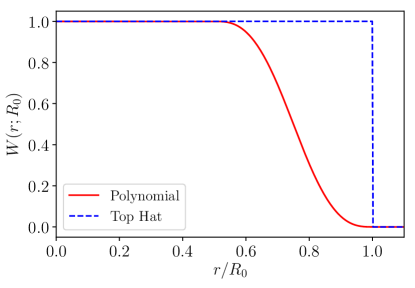
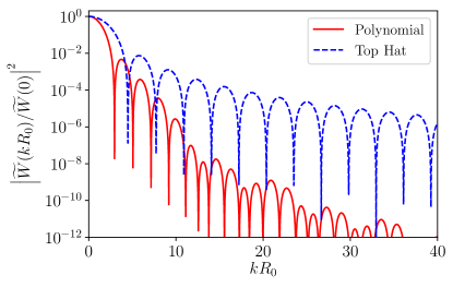
with coefficients chosen to ensure that the function, along with its first and second derivatives, are continuous at the break-points (necessary to avoid broad wings in the Fourier spectrum). The real- and power-space parts of W(𝐫;R0)𝑊𝐫subscript𝑅0W(\mathbf{r};R_{0}) are plotted in Fig. 1 alongside a top-hat window for comparison. By construction, our piecewise-continuous polynomial function has a smooth fall-off with respect to the radial coordinate, but is large for most r=|𝐫|<R0𝑟𝐫subscript𝑅0r=|\mathbf{r}|<R_{0}. The power spectrum of the polynomial window is significantly narrower than that of the top-hat function, with stronger decay with respect to k𝑘k resulting from the greater smoothness in real-space. This leads to reduced bias in the small-scale galaxy power spectrum measurement. In addition, this apodizes the survey-correction factor Φ(r,μ)Φ𝑟𝜇\Phi(r,\mu), both increasing its smoothness and giving zero weight to separations at large r𝑟r where ΦΦ\Phi departs strongly from unity.

Refer to caption
(a) Window Function, W(|𝐫|;R0)𝑊𝐫subscript𝑅0W(|\mathbf{r}|;R_{0})
Refer to caption
(b) Fourier Transformed Window W~(|𝐤|;R0)~𝑊𝐤subscript𝑅0\widetilde{W}(|\mathbf{k}|;R_{0})
Figure 1: Real and Fourier-space plots of the (radial) pair-separation window function WR0subscript𝑊subscript𝑅0W_{R_{0}}. Here, R0subscript𝑅0R_{0} is the truncation scale of the window (typically R0100h1Mpcsimilar-tosubscript𝑅0100superscript1MpcR_{0}\sim 100h^{-1}\mathrm{Mpc}), and we plot both the utilized polynomial window (Eq. 3.1) and a spherical top-hat function. The Fourier space window functions are computed from Hankel transforms of W(𝐫;R0)𝑊𝐫subscript𝑅0W(\mathbf{r};R_{0}) and are here displayed in power-space, normalized by the |𝐤|=0𝐤0|\mathbf{k}|=0 value to aid comparison. We note that the polynomial power spectrum exhibits much stronger fall-off with |𝐤|𝐤|\mathbf{k}| than the top-hat window, due to its smoothness up to the second radial derivative.

Using this window function, the anisotropic power spectrum integral becomes

Pa(R0)subscriptsuperscript𝑃𝑎subscript𝑅0\displaystyle P^{a}_{\ell}(R_{0}) =\displaystyle= 1V(nw)2¯d3𝐫id3𝐫jn(𝐫i)n(𝐫j)w(𝐫i)w(𝐫j)δ(𝐫i)δ(𝐫j)Aa(𝐫i𝐫j)Φ(𝐫i𝐫j)W(𝐫i𝐫j;R0)1𝑉¯superscript𝑛𝑤2superscript𝑑3subscript𝐫𝑖superscript𝑑3subscript𝐫𝑗𝑛subscript𝐫𝑖𝑛subscript𝐫𝑗𝑤subscript𝐫𝑖𝑤subscript𝐫𝑗𝛿subscript𝐫𝑖𝛿subscript𝐫𝑗subscriptsuperscript𝐴𝑎subscript𝐫𝑖subscript𝐫𝑗Φsubscript𝐫𝑖subscript𝐫𝑗𝑊subscript𝐫𝑖subscript𝐫𝑗subscript𝑅0\displaystyle\frac{1}{V\overline{(nw)^{2}}}\int d^{3}\mathbf{r}_{i}\,d^{3}\mathbf{r}_{j}\,n(\mathbf{r}_{i})n(\mathbf{r}_{j})w(\mathbf{r}_{i})w(\mathbf{r}_{j})\delta(\mathbf{r}_{i})\delta(\mathbf{r}_{j})A^{a}_{\ell}(\mathbf{r}_{i}-\mathbf{r}_{j})\Phi(\mathbf{r}_{i}-\mathbf{r}_{j})W(\mathbf{r}_{i}-\mathbf{r}_{j};R_{0}) (3.2)

with =00\ell=0 giving the isotropic estimator. This converges to the true power, Pasuperscriptsubscript𝑃𝑎P_{\ell}^{a}, in the limit R0subscript𝑅0R_{0}\rightarrow\infty. This may again be computed using pair-counting, where the pair-counts are now defined as

XY~R0a=iXjY,ij if X=YwiwjAijaΦijWijR0subscriptsuperscript~𝑋𝑌𝑎subscript𝑅0subscript𝑖𝑋subscriptformulae-sequence𝑗𝑌𝑖𝑗 if 𝑋𝑌subscript𝑤𝑖subscript𝑤𝑗subscriptsuperscript𝐴𝑎𝑖𝑗subscriptΦ𝑖𝑗superscriptsubscript𝑊𝑖𝑗subscript𝑅0\displaystyle\widetilde{XY}^{a}_{R_{0}}=\sum_{i\in X}\sum_{j\in Y,i\neq j\text{ if }X=Y}w_{i}w_{j}A^{a}_{ij}\Phi_{ij}W_{ij}^{R_{0}} (3.3)

for X,Y[D,R]𝑋𝑌𝐷𝑅X,Y\in[D,R], drawing i𝑖i from X𝑋X and j𝑗j from Y𝑌Y. Here AijaAa(𝐫i𝐫j)subscriptsuperscript𝐴𝑎𝑖𝑗superscript𝐴𝑎subscript𝐫𝑖subscript𝐫𝑗A^{a}_{ij}\equiv A^{a}(\mathbf{r}_{i}-\mathbf{r}_{j}) and WijR0W(𝐫i𝐫j;R0)subscriptsuperscript𝑊subscript𝑅0𝑖𝑗𝑊subscript𝐫𝑖subscript𝐫𝑗subscript𝑅0W^{R_{0}}_{ij}\equiv W(\mathbf{r}_{i}-\mathbf{r}_{j};R_{0}).

3.2 Power Spectrum Modification

The windowed 3D power spectrum, P(𝐤;R0)𝑃𝐤subscript𝑅0P(\mathbf{k};R_{0}), may be written using Eq. 2.1 as

P(𝐤;R0)𝑃𝐤subscript𝑅0\displaystyle P(\mathbf{k};R_{0}) =\displaystyle= 1V(nw)2¯d3𝐫id3𝐫jn(𝐫i)n(𝐫j)w(𝐫i)w(𝐫j)δ(𝐫i)δ(𝐫j)ei𝐤(𝐫i𝐫j)Φ(𝐫i𝐫j)W(𝐫i𝐫j;R0)1𝑉¯superscript𝑛𝑤2superscript𝑑3subscript𝐫𝑖superscript𝑑3subscript𝐫𝑗𝑛subscript𝐫𝑖𝑛subscript𝐫𝑗𝑤subscript𝐫𝑖𝑤subscript𝐫𝑗𝛿subscript𝐫𝑖𝛿subscript𝐫𝑗superscript𝑒𝑖𝐤subscript𝐫𝑖subscript𝐫𝑗Φsubscript𝐫𝑖subscript𝐫𝑗𝑊subscript𝐫𝑖subscript𝐫𝑗subscript𝑅0\displaystyle\frac{1}{V\overline{(nw)^{2}}}\int d^{3}\mathbf{r}_{i}\,d^{3}\mathbf{r}_{j}\,n(\mathbf{r}_{i})n(\mathbf{r}_{j})w(\mathbf{r}_{i})w(\mathbf{r}_{j})\delta(\mathbf{r}_{i})\delta(\mathbf{r}_{j})\,e^{i\mathbf{k}\cdot(\mathbf{r}_{i}-\mathbf{r}_{j})}\Phi(\mathbf{r}_{i}-\mathbf{r}_{j})W(\mathbf{r}_{i}-\mathbf{r}_{j};R_{0})
=\displaystyle= 1V(nw)2¯d3𝐫id3𝐫jn(𝐫i)n(𝐫j)w(𝐫i)w(𝐫j)δ(𝐫i)δ(𝐫j)Φ(𝐫i𝐫j)d3𝐩(2π)3ei(𝐤𝐩)(𝐫i𝐫j)W~(𝐩;R0)1𝑉¯superscript𝑛𝑤2superscript𝑑3subscript𝐫𝑖superscript𝑑3subscript𝐫𝑗𝑛subscript𝐫𝑖𝑛subscript𝐫𝑗𝑤subscript𝐫𝑖𝑤subscript𝐫𝑗𝛿subscript𝐫𝑖𝛿subscript𝐫𝑗Φsubscript𝐫𝑖subscript𝐫𝑗superscript𝑑3𝐩superscript2𝜋3superscript𝑒𝑖𝐤𝐩subscript𝐫𝑖subscript𝐫𝑗~𝑊𝐩subscript𝑅0\displaystyle\frac{1}{V\overline{(nw)^{2}}}\int d^{3}\mathbf{r}_{i}\,d^{3}\mathbf{r}_{j}\,n(\mathbf{r}_{i})n(\mathbf{r}_{j})w(\mathbf{r}_{i})w(\mathbf{r}_{j})\delta(\mathbf{r}_{i})\delta(\mathbf{r}_{j})\Phi(\mathbf{r}_{i}-\mathbf{r}_{j})\int\frac{d^{3}\mathbf{p}}{(2\pi)^{3}}e^{i(\mathbf{k}-\mathbf{p})\cdot(\mathbf{r}_{i}-\mathbf{r}_{j})}\widetilde{W}(\mathbf{p};R_{0})
=\displaystyle= d3𝐩(2π)3P(𝐤𝐩)W~(𝐩;R0)=1(2π)3[PW~R0](𝐤)=[ξ(𝐫)W(𝐫;R0)](𝐤).superscript𝑑3𝐩superscript2𝜋3𝑃𝐤𝐩~𝑊𝐩subscript𝑅01superscript2𝜋3delimited-[]𝑃subscript~𝑊subscript𝑅0𝐤delimited-[]𝜉𝐫𝑊𝐫subscript𝑅0𝐤\displaystyle\int\frac{d^{3}\mathbf{p}}{(2\pi)^{3}}\,P(\mathbf{k}-\mathbf{p})\widetilde{W}(\mathbf{p};R_{0})=\frac{1}{(2\pi)^{3}}\left[P\ast\widetilde{W}_{R_{0}}\right](\mathbf{k})=\mathcal{F}\left[\xi(\mathbf{r})W(\mathbf{r};R_{0})\right](\mathbf{k}).

Here we have expressed W(𝐫i𝐫j;R0)𝑊subscript𝐫𝑖subscript𝐫𝑗subscript𝑅0W(\mathbf{r}_{i}-\mathbf{r}_{j};R_{0}) in terms of its Fourier transform, noting that this gives a simple convolution of the true power, P(𝐤)𝑃𝐤P(\mathbf{k}), with the Fourier-transformed window function W~R0(𝐤)subscript~𝑊subscript𝑅0𝐤\widetilde{W}_{R_{0}}(\mathbf{k}). For the isotropic case, integrating over ΩksubscriptΩ𝑘\Omega_{k} gives

P(k;R0)𝑃𝑘subscript𝑅0\displaystyle P(k;R_{0}) =\displaystyle= 1(2π)3dΩk4π[PW~R0](𝐤)1superscript2𝜋3𝑑subscriptΩ𝑘4𝜋delimited-[]𝑃subscript~𝑊subscript𝑅0𝐤\displaystyle\frac{1}{(2\pi)^{3}}\int\frac{d\Omega_{k}}{4\pi}\left[P\ast\widetilde{W}_{R_{0}}\right](\mathbf{k}) (3.5)

which may be written in terms of the isotropic 2PCF ξ(r)𝜉𝑟\xi(r) and the (radial) W(𝐫;R0)𝑊𝐫subscript𝑅0W(\mathbf{r};R_{0}) function as

P(k;R0)𝑃𝑘subscript𝑅0\displaystyle P(k;R_{0}) =\displaystyle= dΩk4πd3𝐫ei𝐤𝐫ξ(𝐫)W(𝐫;R0)=12𝑑μkd3𝐫eikrμkξ(𝐫)W(𝐫;R0)𝑑subscriptΩ𝑘4𝜋superscript𝑑3𝐫superscript𝑒𝑖𝐤𝐫𝜉𝐫𝑊𝐫subscript𝑅012differential-dsubscript𝜇𝑘superscript𝑑3𝐫superscript𝑒𝑖𝑘𝑟subscript𝜇𝑘𝜉𝐫𝑊𝐫subscript𝑅0\displaystyle\int\frac{d\Omega_{k}}{4\pi}\int d^{3}\mathbf{r}\,e^{i\mathbf{k}\cdot\mathbf{r}}\xi(\mathbf{r})W(\mathbf{r};R_{0})=\frac{1}{2}\int d\mu_{k}\int d^{3}\mathbf{r}\,e^{ikr\mu_{k}}\xi(\mathbf{r})W(\mathbf{r};R_{0})
=\displaystyle= 0r2𝑑r11𝑑μr02π𝑑ϕrj0(kr)ξ(r,μr)W(r;R0)=4π0r2𝑑rξ(r)W(r;R0)j0(kr)superscriptsubscript0superscript𝑟2differential-d𝑟superscriptsubscript11differential-dsubscript𝜇𝑟superscriptsubscript02𝜋differential-dsubscriptitalic-ϕ𝑟subscript𝑗0𝑘𝑟𝜉𝑟subscript𝜇𝑟𝑊𝑟subscript𝑅04𝜋superscriptsubscript0superscript𝑟2differential-d𝑟𝜉𝑟𝑊𝑟subscript𝑅0subscript𝑗0𝑘𝑟\displaystyle\int_{0}^{\infty}r^{2}dr\,\int_{-1}^{1}d\mu_{r}\,\int_{0}^{2\pi}d\phi_{r}\,j_{0}(kr)\xi(r,\mu_{r})W(r;R_{0})=4\pi\int_{0}^{\infty}r^{2}dr\,\xi(r)W(r;R_{0})j_{0}(kr)

(before radial binning), where j0subscript𝑗0j_{0} is a zeroth-order spherical Bessel function of the first kind. Here we have aligned 𝐤𝐤\mathbf{k} with 𝐫𝐫\mathbf{r} in the first line (such that 𝐤𝐫=krμk𝐤𝐫𝑘𝑟subscript𝜇𝑘\mathbf{k}\cdot\mathbf{r}=kr\mu_{k}) and noted that 11𝑑μrξ(r,μr)=ξ(r)superscriptsubscript11differential-dsubscript𝜇𝑟𝜉𝑟subscript𝜇𝑟𝜉𝑟\int_{-1}^{1}d\mu_{r}\xi(r,\mu_{r})=\xi(r). (This is also derived as the =00\ell=0 case of the result of appendix B for A(𝐫)=ξ(𝐫)W(𝐫;R0)𝐴𝐫𝜉𝐫𝑊𝐫subscript𝑅0A(\mathbf{r})=\xi(\mathbf{r})W(\mathbf{r};R_{0}), A~(𝐤)=P(𝐤;R0)~𝐴𝐤𝑃𝐤subscript𝑅0\widetilde{A}(\mathbf{k})=P(\mathbf{k};R_{0}).) This simple form will be used below to assess the effects of the polynomial window on the measured power spectrum.

For the anisotropic power spectrum multipoles, we adopt a similar approach, computing the angular integrals of P(𝐤)𝑃𝐤P(\mathbf{k}) weighted by Legendre polynomials. Notably, these depend on the LoS of a particular pair of points, 𝐱=12(𝐫i+𝐫j)𝐱12subscript𝐫𝑖subscript𝐫𝑗\mathbf{x}=\tfrac{1}{2}(\mathbf{r}_{i}+\mathbf{r}_{j}), thus we must integrate over ΩksubscriptΩ𝑘\Omega_{k} before averaging over the LoS of galaxy pairs. This is made possible by noting that the quantities ξ(𝐫)W(𝐫;R0)𝜉𝐫𝑊𝐫subscript𝑅0\xi(\mathbf{r})W(\mathbf{r};R_{0}) appearing in Eq. 3.2 are strictly the integrals of ξ(𝐫;𝐱)W(𝐫;R0)𝜉𝐫𝐱𝑊𝐫subscript𝑅0\xi(\mathbf{r};\mathbf{x})W(\mathbf{r};R_{0}) over 𝐱𝐱\mathbf{x}, where ξ(𝐫;𝐱)𝜉𝐫𝐱\xi(\mathbf{r};\mathbf{x}) is the local 2PCF measurement for galaxies at mid-point 𝐱𝐱\mathbf{x}. Using the linearity of Fourier transforms to switch the order of integration we obtain

P(k;R0)subscript𝑃𝑘subscript𝑅0\displaystyle P_{\ell}(k;R_{0}) =\displaystyle= (2+1)d3𝐱VdΩk4π[ξ(𝐫;𝐱)W(𝐫;R0)]L(𝐤^𝐱^)21superscript𝑑3𝐱𝑉𝑑subscriptΩ𝑘4𝜋delimited-[]𝜉𝐫𝐱𝑊𝐫subscript𝑅0subscript𝐿^𝐤^𝐱\displaystyle(2\ell+1)\int\frac{d^{3}\mathbf{x}}{V}\int\frac{d\Omega_{k}}{4\pi}\mathcal{F}\left[\xi(\mathbf{r};\mathbf{x})W(\mathbf{r};R_{0})\right]L_{\ell}(\hat{\mathbf{k}}\cdot\hat{\mathbf{x}})
=\displaystyle= 1(2π)3d3𝐱V{(2+1)dΩk4π[PW~](𝐤)L(𝐤^𝐱^)}=1(2π)3[PW~](k)1superscript2𝜋3superscript𝑑3𝐱𝑉21𝑑subscriptΩ𝑘4𝜋delimited-[]𝑃~𝑊𝐤subscript𝐿^𝐤^𝐱1superscript2𝜋3delimited-⟨⟩subscriptdelimited-[]𝑃~𝑊𝑘\displaystyle\frac{1}{(2\pi)^{3}}\int\frac{d^{3}\mathbf{x}}{V}\left\{(2\ell+1)\int\frac{d\Omega_{k}}{4\pi}\left[P\ast\widetilde{W}\right](\mathbf{k})L_{\ell}(\hat{\mathbf{k}}\cdot\hat{\mathbf{x}})\right\}=\frac{1}{(2\pi)^{3}}\left\langle{}\left[P\ast\widetilde{W}\right]_{\ell}\right\rangle(k)

thus the power spectrum multipoles are simply related to the multipoles of the convolution of P(𝐤)𝑃𝐤P(\mathbf{k}) and W~(𝐤)~𝑊𝐤\widetilde{W}(\mathbf{k}) (with angle brackets indicating averaging over the LoS). Although this result has been derived for a LoS angle convention (choosing 𝐱𝐱\mathbf{x} to be the mid-point of the two galaxies), it applies equally well to other conventions, e.g. the Yamamoto et al. (2006) approximation, setting 𝐱=𝐫j𝐱subscript𝐫𝑗\mathbf{x}=\mathbf{r}_{j} or the flat-sky approximation, with 𝐱=const.𝐱const\mathbf{x}=\mathrm{const.}

Analogous to the isotropic case, P(k;R0)subscript𝑃𝑘subscript𝑅0P_{\ell}(k;R_{0}) may be expressed in terms of the 2PCF multipoles ξ(r)subscript𝜉𝑟\xi_{\ell}(r), noting that the power spectrum multipoles are those of the Fourier transform of ξ(𝐫)W(𝐫;R0)𝜉𝐫𝑊𝐫subscript𝑅0\xi(\mathbf{r})W(\mathbf{r};R_{0}). In appendix B, we show that the configuration- and Fourier-space multipoles of a function A(𝐫)𝐴𝐫A(\mathbf{r}) are related by

A~(k)=4πi0r2𝑑rA(r)j(kr)subscript~𝐴𝑘4𝜋superscript𝑖superscriptsubscript0superscript𝑟2differential-d𝑟subscript𝐴𝑟subscript𝑗𝑘𝑟\displaystyle\widetilde{A}_{\ell}(k)=4\pi i^{\ell}\int_{0}^{\infty}r^{2}dr\,A_{\ell}(r)j_{\ell}(kr) (3.8)

(applicable both for fixed and moving lines-of-sight); setting A(𝐫)=ξ(𝐫)W(𝐫;R0)𝐴𝐫𝜉𝐫𝑊𝐫subscript𝑅0A(\mathbf{r})=\xi(\mathbf{r})W(\mathbf{r};R_{0}) and hence A~(𝐤)=P(𝐤;R0)~𝐴𝐤𝑃𝐤subscript𝑅0\widetilde{A}(\mathbf{k})=P(\mathbf{k};R_{0}) implies

P(k;R0)=4πi0r2𝑑rξ(r)W(r;R0)j(kr)subscript𝑃𝑘subscript𝑅04𝜋superscript𝑖superscriptsubscript0superscript𝑟2differential-d𝑟subscript𝜉𝑟𝑊𝑟subscript𝑅0subscript𝑗𝑘𝑟\displaystyle P_{\ell}(k;R_{0})=4\pi i^{\ell}\int_{0}^{\infty}r^{2}dr\,\xi_{\ell}(r)W(r;R_{0})j_{\ell}(kr) (3.9)

since [ξ(𝐫)W(𝐫;R0)]=ξ(r)W(r;R0)subscriptdelimited-[]𝜉𝐫𝑊𝐫subscript𝑅0subscript𝜉𝑟𝑊𝑟subscript𝑅0\left[\xi(\mathbf{r})W(\mathbf{r};R_{0})\right]_{\ell}=\xi_{\ell}(r)W(r;R_{0}), due to W𝑊W being isotropic. Notably, there is no multipole mixing induced by our pair-separation window function.

3.3 Assessing the Impact of the Pair-Separation Limit R0subscript𝑅0R_{0}

From Eqs. 3.2 & 3.9 we can predict the effects of the window function on measurements of the power spectrum multipoles for various k𝑘k. Here, we assume an ideal infinite survey (such that n,w𝑛𝑤n,w are constant and Φ(𝐫)=1Φ𝐫1\Phi(\mathbf{r})=1 for all 𝐫𝐫\mathbf{r}), using a smooth 2PCF input derived from Hankel transforms of a matter power spectrum computed in CAMB888camb.info (Lewis & Bridle, 2002). For simplicity, we assume a linear power spectrum at redshift z=0.57𝑧0.57z=0.57 with the cosmology {Ωb=0.048,ΩΛ=0.71,h=0.7}formulae-sequencesubscriptΩ𝑏0.048formulae-sequencesubscriptΩΛ0.710.7\{\Omega_{b}=0.048,\Omega_{\Lambda}=0.71,h=0.7\}, but add Kaiser redshift space distortions (RSD) to create a non-trivial quadrupole and hexadecapole. We adopt Kaiser parameter β=0.774𝛽0.774\beta=0.774 and bias b=2𝑏2b=2 to emulate the BOSS DR12 CMASS sample (Gil-Marín et al., 2016a). No Finger-of-God (FoG) effects are included in this 2PCF since they are more difficult to model. Although the model is clearly not representative of the true P(k)subscript𝑃𝑘P_{\ell}(k), we expected it to be a good predictor of pair-separation window function biases.

In Fig. 2 we plot the ratio of windowed to true anisotropic power as a function of k𝑘k for three sets of multipoles \ell and truncation radii, obtained from numerical integration of Eq. 3.9. Notably there is a significant overestimate (underestimate) of monopole (quadrupole and hexadecapole) power on large scales (small k𝑘k) when using the window function, but the ratio converges to unity at large k𝑘k. Broader window functions are seen to have a smaller impact on the windowed power spectrum, as expected, and the impact is seen to be more significant at higher multipoles. For R0100h1Mpcgreater-than-or-equivalent-tosubscript𝑅0100superscript1MpcR_{0}\gtrsim 100h^{-1}\mathrm{Mpc}, we obtain sub-percent agreement between windowed and true power for k0.2hMpc1greater-than-or-equivalent-to𝑘0.2superscriptMpc1k\gtrsim 0.2h\,\mathrm{Mpc}^{-1}, indicating that our estimator will work well in this regime. In addition, we note that these plots do not include k𝑘k-space binning; using wide k𝑘k bins will reduce the oscillatory behaviour of P(k;R0)/P(k)subscript𝑃𝑘subscript𝑅0subscript𝑃𝑘P_{\ell}(k;R_{0})/P_{\ell}(k) with respect to k𝑘k and hence give improve the accuracy with which power can be measured.

Refer to caption
Refer to caption
Figure 2: Comparison of windowed to true power spectrum moments using the polynomial window function (Eq. 3.1), computed for various multipoles and truncation scales, R0subscript𝑅0R_{0} (in h1Mpcsuperscript1Mpch^{-1}\mathrm{Mpc}). The upper and lower plots show the same data on logarithmic and linear scales respectively. Forecasts are obtained for a uniform unbounded survey (with correction function Φ=1Φ1\Phi=1 everywhere), utilizing a smooth two-point correlation function derived from the linear matter power spectrum at z=0.57𝑧0.57z=0.57 (from CAMB), with anisotropies included solely via the Kaiser redshift-space distortion (RSD) prescription, noting that we expect only weak dependence on the exact form of the power spectrum. For all multipoles, the windowed power matches the true power to high accuracy at large k𝑘k, but we observe larger deviations at small k𝑘k, especially for higher multipoles. For R0100h1Mpcgreater-than-or-equivalent-tosubscript𝑅0100superscript1MpcR_{0}\gtrsim 100h^{-1}\mathrm{Mpc}, we achieve sub-percent accuracy with the windowed power spectrum on scales k>0.2hMpc1𝑘0.2superscriptMpc1k>0.2h\,\mathrm{Mpc}^{-1}.

4 Dependence on Survey Geometry

The survey-correction function Φ(𝐫)=RRideal(𝐫)/RR(𝐫)Φ𝐫𝑅subscript𝑅ideal𝐫𝑅𝑅𝐫\Phi(\mathbf{r})=RR_{\mathrm{ideal}}(\mathbf{r})/RR(\mathbf{r}) (Eq. 2.4) allows us to assess the impact of the survey geometry on the measured power spectrum. First, recall that our (boundary corrected) power spectrum estimator is derived simply from the Fourier transform of the Landy & Szalay (1993) estimator, i.e.

P(𝐤)=[NN(𝐫)RR(𝐫)](𝐤)𝑃𝐤delimited-[]𝑁𝑁𝐫𝑅𝑅𝐫𝐤\displaystyle P(\mathbf{k})=\mathcal{F}\left[\frac{NN(\mathbf{r})}{RR(\mathbf{r})}\right](\mathbf{k}) (4.1)

(cf. Eq. 2.1, here ignoring the pair-count window). If we had instead used the FKP estimator (Eq. 2.7), we would have measured

Puncorr(𝐤)=[NN(𝐫)RRideal(𝐫)]=[NN(𝐫)RR(𝐫)Φ(𝐫)]=[ξ(𝐫)Φ1(𝐫)]=1(2π)3[P[Φ1]](𝐤)superscript𝑃uncorr𝐤delimited-[]𝑁𝑁𝐫𝑅subscript𝑅ideal𝐫delimited-[]𝑁𝑁𝐫𝑅𝑅𝐫Φ𝐫delimited-[]𝜉𝐫superscriptΦ1𝐫1superscript2𝜋3delimited-[]𝑃delimited-[]superscriptΦ1𝐤\displaystyle P^{\mathrm{uncorr}}(\mathbf{k})=\mathcal{F}\left[\frac{NN(\mathbf{r})}{RR_{\mathrm{ideal}}(\mathbf{r})}\right]=\mathcal{F}\left[\frac{NN(\mathbf{r})}{RR(\mathbf{r})\Phi(\mathbf{r})}\right]=\mathcal{F}\left[\xi(\mathbf{r})\Phi^{-1}(\mathbf{r})\right]=\frac{1}{(2\pi)^{3}}\left[P\ast\mathcal{F}[\Phi^{-1}]\right](\mathbf{k}) (4.2)

applying the convolution theorem and noting that the factor I=V(nw)2¯𝐼𝑉¯superscript𝑛𝑤2I=V\overline{(nw)^{2}} appearing in the denominator of the FKP estimator is simply the idealized survey pair-counts. The uncorrected power spectrum is thus a convolution of the corrected power with the Fourier transform of the reciprocal correction function. With the inclusion of the pair-wise window function, both Puncorr(𝐤)superscript𝑃uncorr𝐤P^{\mathrm{uncorr}}(\mathbf{k}) and P(𝐤)𝑃𝐤P(\mathbf{k}) are further convolved with W~(𝐤;R0)~𝑊𝐤subscript𝑅0\widetilde{W}(\mathbf{k};R_{0}).

To investigate this, we consider the expansion of Puncorrsuperscript𝑃uncorrP^{\mathrm{\,uncorr}} into Legendre multipoles, utilizing the result of appendix C, which states that, for an arbitrary function ω(𝐫)𝜔𝐫\omega(\mathbf{r}), the multipoles of 𝒫(𝐤)=[ξ(𝐫)ω(𝐫)]𝒫𝐤delimited-[]𝜉𝐫𝜔𝐫\mathcal{P}(\mathbf{k})=\mathcal{F}\left[\xi(\mathbf{r})\omega(\mathbf{r})\right] are given by

𝒫(k)subscript𝒫𝑘\displaystyle\mathcal{P}_{\ell}(k) =\displaystyle= (2+1)1,2(12000)2𝒢;1,2(k)21subscriptsubscript1subscript2superscriptsubscript1subscript20002subscript𝒢subscript1subscript2𝑘\displaystyle(2\ell+1)\sum_{\ell_{1},\ell_{2}}\left(\begin{array}[]{ccc}\ell_{1}&\ell_{2}&\ell\\ 0&0&0\end{array}\right)^{2}\mathcal{G}_{\ell;\ell_{1},\ell_{2}}(k) (4.5)
𝒢;1,2(k)subscript𝒢subscript1subscript2𝑘\displaystyle\mathcal{G}_{\ell;\ell_{1},\ell_{2}}(k) =\displaystyle= 4πi0r2𝑑rj(kr)ξ1(r)ω2(r).4𝜋superscript𝑖superscriptsubscript0superscript𝑟2differential-d𝑟subscript𝑗𝑘𝑟subscript𝜉subscript1𝑟subscript𝜔subscript2𝑟\displaystyle 4\pi i^{\ell}\int_{0}^{\infty}r^{2}dr\,\,j_{\ell}(kr)\xi_{\ell_{1}}(r)\omega_{\ell_{2}}(r).

in terms of a Wigner 3j3𝑗3j symbol (NIST, DLMF, Sec. 34.2), with the summations over 1subscript1\ell_{1} and 2subscript2\ell_{2} restricted to those values allowed by the 3j3𝑗3j selection rules. This applies to both constant and moving lines-of-sight. Here ω(𝐫)=Φ1(𝐫)W(𝐫;R0)𝜔𝐫superscriptΦ1𝐫𝑊𝐫subscript𝑅0\omega(\mathbf{r})=\Phi^{-1}(\mathbf{r})W(\mathbf{r};R_{0}) (reintroducing the pair-separation window function) giving

Puncorr(k;R0)subscriptsuperscript𝑃uncorr𝑘subscript𝑅0\displaystyle P^{\mathrm{uncorr}}_{\ell}(k;R_{0}) =\displaystyle= (2+1)12(12000)2;1,2(k;R0)21subscriptsubscript1subscript2superscriptsubscript1subscript20002subscriptsubscript1subscript2𝑘subscript𝑅0\displaystyle(2\ell+1)\sum_{\ell_{1}\ell_{2}}\left(\begin{array}[]{ccc}\ell&\ell_{1}&\ell_{2}\\ 0&0&0\\ \end{array}\right)^{2}\mathcal{H}_{\ell;\ell_{1},\ell_{2}}(k;R_{0}) (4.8)
;1,2(k;R0)subscriptsubscript1subscript2𝑘subscript𝑅0\displaystyle\mathcal{H}_{\ell;\ell_{1},\ell_{2}}(k;R_{0}) =\displaystyle= 4πi0r2𝑑rξ1(r)[Φ1]2(r)W(r;R0)j(kr)4𝜋superscript𝑖superscriptsubscript0superscript𝑟2differential-d𝑟subscript𝜉subscript1𝑟subscriptdelimited-[]superscriptΦ1subscript2𝑟𝑊𝑟subscript𝑅0subscript𝑗𝑘𝑟\displaystyle 4\pi i^{\ell}\int_{0}^{\infty}r^{2}dr\,\xi_{\ell_{1}}(r)[\Phi^{-1}]_{\ell_{2}}(r)W(r;R_{0})j_{\ell}(kr)

which may be compared with Eq. 3.9, which defines P(k;R0)subscript𝑃𝑘subscript𝑅0P_{\ell}(k;R_{0}). This clearly shows how ignoring the survey correction function ΦΦ\Phi introduces bias and multipole mixing into the windowed power spectrum.

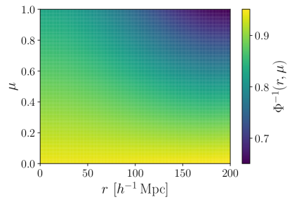
To illustrate this, we consider the corrected and uncorrected power using a survey correction function, ΦΦ\Phi, appropriate for the BOSS DR12 CMASS-N dataset (Dawson et al., 2013). This is computed by measuring the true RR𝑅𝑅RR pair-counts in 400 radial and 100 angular bins via exhaustive pair-counting using corrfunc and comparing these to the expected value, given the normalization of V(nw)2¯53h3Mpc3𝑉¯superscript𝑛𝑤253superscript3superscriptMpc3V\overline{(nw)^{2}}\approx 53h^{3}\,\mathrm{Mpc}^{-3}. The observed values of Φ1superscriptΦ1\Phi^{-1} (defined by Eq. 2.5) are then fit with spline curves in Legendre multipole space, giving a smooth Φ(r,μ)Φ𝑟𝜇\Phi(r,\mu) representation. In Fig. 3, we show Φ1superscriptΦ1\Phi^{-1} as a function of spatial position. As expected, Φ11superscriptΦ11\Phi^{-1}\rightarrow 1 on small radial scales (when few pairs cross the survey boundary), but Φ1superscriptΦ1\Phi^{-1} is reduced at larger r𝑟r, especially for pairs parallel to the LoS μ1𝜇1\mu\approx 1, since these pairs are more likely to cross the survey boundary. Φ1(r,μ)superscriptΦ1𝑟𝜇\Phi^{-1}(r,\mu) is clearly observed to be smooth here.
Refer to caption
Figure 3: Reciprocal of the survey-correction function Φ(𝐫)Φ𝐫\Phi(\mathbf{r}) for the BOSS DR12 CMASS-N survey (Dawson et al., 2013) as a function of distance and angle of a particle pair from the LoS. Φ1superscriptΦ1\Phi^{-1} is the ratio of the true RR𝑅𝑅RR pair-counts (computed from exhaustive pair-counting with corrfunc (Sinha & Garrison, 2017)) to those expected for a uniform, infinite survey, and deviations from unity show the effects of the survey geometry. As expected, deviations are largest for widely separated pairs oriented along the LoS. This plot is generated by fitting smooth splines to the Legendre moments of the measured grid of ΦΦ\Phi values.

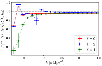
Using a smooth mock 2PCF derived from a linear power spectrum with RSD added via the Kaiser prescription (as in Sec. 3.3), we may compute the ratio of uncorrected to corrected power via Eqs. 4.8 & 3.9, utilizing the Legendre multipoles of Φ1superscriptΦ1\Phi^{-1} (up to =66\ell=6) used to create Fig. 3. Fig. 4 shows this, with numerical integration used to evaluate the power integrals for various k𝑘k and multipoles [0,2,4]024\ell\in[0,2,4]. On the large scales probed here, we note only small effects on the isotropic power spectrum (=00\ell=0), at the sub-percent level for k0.2hMpc1greater-than-or-equivalent-to𝑘0.2superscriptMpc1k\gtrsim 0.2h\,\mathrm{Mpc}^{-1}. For higher multipoles, the difference between the corrected and uncorrected power is more striking, with the quadrupole (hexadecapole) measurements differing at the 1%percent11\% (20%percent2020\%) level for k0.2hMpc1𝑘0.2superscriptMpc1k\approx 0.2h\,\mathrm{Mpc}^{-1}. The large difference in the measured hexadecapole is as expected since the hexadecapole is intrinsically a very small signal. It is clear, therefore, that proper consideration of the survey window functions is needed even on small scales. Standard Fourier transform approaches must do this via deconvolution with the survey mask power spectrum; our method here differs since it is performed directly as the power is estimated, not in post-processing. Although the results above are presented for a specific linear power spectrum, we do not expect them to have strong dependence on the exact power spectrum form.

Refer to caption
Figure 4: Comparison of the survey-geometry uncorrected and corrected measured power spectrum multipoles for simulated observations of the BOSS DR12 CMASS-N region, using a mock correlation function computed from a linear power spectrum in CAMB (Lewis & Bridle, 2002) with Kaiser RSD anisotropies added. We note that the high-k𝑘k uncorrected power spectrum is equivalent to that used in Bianchi et al. (2015) (or Feldman et al. (1994) for the monopole) without any deconvolution. The two plots are identical, but with different scales. These are derived from Eqs. 4.8 & 3.9, using a polynomial pair-separation window function truncated at 200h1Mpc200superscript1Mpc200h^{-1}\mathrm{Mpc}, with the inclusion of the reciprocal survey correction factor Φ1superscriptΦ1\Phi^{-1} (shown in Fig. 3) in the uncorrected power spectrum accounting for the lack of consideration of the survey-geometry. To account for small errors (at the few percent level) in the normalization of ΦΦ\Phi, the curves are normalized by their power at k=2𝑘2k=2 (where the geometry should have no significant effect). We note significant deviations from unity on small scales, especially for higher multipoles. Fig. 7 gives the analogous plot applied to full simulated galaxy catalogs.

5 Power Spectrum Covariances

One motivation for estimating power spectra in configuration-space is the ability to generate survey-dependent covariance matrices using the techniques developed for correlation function covariances. In addition, computing the power spectrum and 2PCF in the same manner means that we can compute cross-covariances between statistics, facilitating robust joint analyses that will be important in upcoming galaxy surveys. We here discuss the form and implementation of these covariances, noting that they are fully analogous to the 2PCF and 3PCF covariances first presented in O’Connell et al. (2016) and Philcox & Eisenstein (2019), with the addition of pair-wise window functions and a modified kernel.

5.1 Theoretical Covariance Estimators

5.1.1 Autocovariance of P(k)subscript𝑃𝑘P_{\ell}(k)

The covariance matrix of the windowed anisotropic power spectrum for an arbitrary survey geometry may be derived directly from our estimators (Eq. 3.2). We begin by writing the power spectrum estimator in discrete form;

P^a=1V(nw)2¯ijninjwiwjδiδjA,ijaΦijWijR0superscriptsubscript^𝑃𝑎1𝑉¯superscript𝑛𝑤2subscript𝑖𝑗subscript𝑛𝑖subscript𝑛𝑗subscript𝑤𝑖subscript𝑤𝑗subscript𝛿𝑖subscript𝛿𝑗subscriptsuperscript𝐴𝑎𝑖𝑗subscriptΦ𝑖𝑗superscriptsubscript𝑊𝑖𝑗subscript𝑅0\displaystyle\hat{P}_{\ell}^{a}=\frac{1}{V\overline{(nw)^{2}}}\sum_{i\neq j}n_{i}n_{j}w_{i}w_{j}\delta_{i}\delta_{j}A^{a}_{\ell,ij}\Phi_{ij}W_{ij}^{R_{0}} (5.1)

where the summations are over small volumes containing at most one galaxy and subscripts denote the function arguments, e.g. δiδ(𝐫i)subscript𝛿𝑖𝛿subscript𝐫𝑖\delta_{i}\equiv\delta(\mathbf{r}_{i}) and ΦijΦ(𝐫i𝐫j)subscriptΦ𝑖𝑗Φsubscript𝐫𝑖subscript𝐫𝑗\Phi_{ij}\equiv\Phi(\mathbf{r}_{i}-\mathbf{r}_{j}). Defining the covariance in radial bins a,b𝑎𝑏a,b and Legendre moments p,q𝑝𝑞p,q as

cov(P^pa,P^qb)P^paP^qbP^paP^qbcovsubscriptsuperscript^𝑃𝑎𝑝subscriptsuperscript^𝑃𝑏𝑞delimited-⟨⟩subscriptsuperscript^𝑃𝑎𝑝subscriptsuperscript^𝑃𝑏𝑞delimited-⟨⟩subscriptsuperscript^𝑃𝑎𝑝delimited-⟨⟩subscriptsuperscript^𝑃𝑏𝑞\displaystyle\operatorname{cov}(\hat{P}^{a}_{p}\,,\,\hat{P}^{b}_{q})\equiv\langle{\hat{P}^{a}_{p}\hat{P}^{b}_{q}\rangle}-\langle{\hat{P}^{a}_{p}\rangle}\langle{\hat{P}^{b}_{q}\rangle} (5.2)

(suppressing the R0subscript𝑅0R_{0} truncation radius argument henceforth) we can insert Eq. 5.1 to yield

cov(P^pa,P^qb)=1(V(nw)2¯)2ijklninjnknlwiwjwkwlAp,ijaAq,klbΦijΦklWijR0WklR0[δiδjδkδlδiδjδkδl].covsubscriptsuperscript^𝑃𝑎𝑝subscriptsuperscript^𝑃𝑏𝑞1superscript𝑉¯superscript𝑛𝑤22subscript𝑖𝑗subscript𝑘𝑙subscript𝑛𝑖subscript𝑛𝑗subscript𝑛𝑘subscript𝑛𝑙subscript𝑤𝑖subscript𝑤𝑗subscript𝑤𝑘subscript𝑤𝑙superscriptsubscript𝐴𝑝𝑖𝑗𝑎superscriptsubscript𝐴𝑞𝑘𝑙𝑏subscriptΦ𝑖𝑗subscriptΦ𝑘𝑙subscriptsuperscript𝑊subscript𝑅0𝑖𝑗subscriptsuperscript𝑊subscript𝑅0𝑘𝑙delimited-[]delimited-⟨⟩subscript𝛿𝑖subscript𝛿𝑗subscript𝛿𝑘subscript𝛿𝑙delimited-⟨⟩subscript𝛿𝑖subscript𝛿𝑗delimited-⟨⟩subscript𝛿𝑘subscript𝛿𝑙\displaystyle\operatorname{cov}(\hat{P}^{a}_{p}\,,\,\hat{P}^{b}_{q})=\frac{1}{\left(V\overline{(nw)^{2}}\right)^{2}}\sum_{i\neq j}\sum_{k\neq l}n_{i}n_{j}n_{k}n_{l}w_{i}w_{j}w_{k}w_{l}A_{p,ij}^{a}A_{q,kl}^{b}\Phi_{ij}\Phi_{kl}W^{R_{0}}_{ij}W^{R_{0}}_{kl}\left[\langle{\delta_{i}\delta_{j}\delta_{k}\delta_{l}\rangle}-\langle{\delta_{i}\delta_{j}\rangle}\langle{\delta_{k}\delta_{l}\rangle}\right]. (5.3)

As in O’Connell et al. (2016), the double summation may be expanded into three terms involving two, three and four points in space and we can use Wick’s theorem with the shot-noise contraction approximation δi2(1+δi)/nisuperscriptsubscript𝛿𝑖21subscript𝛿𝑖subscript𝑛𝑖\delta_{i}^{2}\approx(1+\delta_{i})/n_{i} to evaluate the expectation terms arising. This gives the full covariance;

cov(P^pa,P^qb)covsubscriptsuperscript^𝑃𝑎𝑝subscriptsuperscript^𝑃𝑏𝑞\displaystyle\operatorname{cov}(\hat{P}^{a}_{p}\,,\,\hat{P}^{b}_{q}) =\displaystyle= Cpqab4+Cpqab3+Cpqab2superscriptsubscriptsuperscript𝐶𝑎𝑏𝑝𝑞4superscriptsubscriptsuperscript𝐶𝑎𝑏𝑝𝑞3superscriptsubscriptsuperscript𝐶𝑎𝑏𝑝𝑞2\displaystyle{}^{4}C^{ab}_{pq}+{}^{3}C^{ab}_{pq}+{}^{2}C^{ab}_{pq} (5.4)
Cpqab4superscriptsubscriptsuperscript𝐶𝑎𝑏𝑝𝑞4\displaystyle{}^{4}C^{ab}_{pq} =\displaystyle= 1(V(nw)2¯)2ijklninjnknlwiwjwkwlAp,ijaAq,klbΦijΦklWijR0WklR0(ξijkl(4)+2ξikξjl)1superscript𝑉¯superscript𝑛𝑤22subscript𝑖𝑗𝑘𝑙subscript𝑛𝑖subscript𝑛𝑗subscript𝑛𝑘subscript𝑛𝑙subscript𝑤𝑖subscript𝑤𝑗subscript𝑤𝑘subscript𝑤𝑙superscriptsubscript𝐴𝑝𝑖𝑗𝑎superscriptsubscript𝐴𝑞𝑘𝑙𝑏subscriptΦ𝑖𝑗subscriptΦ𝑘𝑙subscriptsuperscript𝑊subscript𝑅0𝑖𝑗subscriptsuperscript𝑊subscript𝑅0𝑘𝑙subscriptsuperscript𝜉4𝑖𝑗𝑘𝑙2subscript𝜉𝑖𝑘subscript𝜉𝑗𝑙\displaystyle\frac{1}{\left(V\overline{(nw)^{2}}\right)^{2}}\sum_{i\neq j\neq k\neq l}n_{i}n_{j}n_{k}n_{l}w_{i}w_{j}w_{k}w_{l}A_{p,ij}^{a}A_{q,kl}^{b}\Phi_{ij}\Phi_{kl}W^{R_{0}}_{ij}W^{R_{0}}_{kl}\left(\xi^{(4)}_{ijkl}+2\xi_{ik}\xi_{jl}\right)
Cpqab3superscriptsubscriptsuperscript𝐶𝑎𝑏𝑝𝑞3\displaystyle{}^{3}C^{ab}_{pq} =\displaystyle= 4×1(V(nw)2¯)2ijkninjnkwi(wj)2wkAp,ijaAq,jkbΦijΦjkWijR0WjkR0(ζijk+ξik)41superscript𝑉¯superscript𝑛𝑤22subscript𝑖𝑗𝑘subscript𝑛𝑖subscript𝑛𝑗subscript𝑛𝑘subscript𝑤𝑖superscriptsubscript𝑤𝑗2subscript𝑤𝑘superscriptsubscript𝐴𝑝𝑖𝑗𝑎superscriptsubscript𝐴𝑞𝑗𝑘𝑏subscriptΦ𝑖𝑗subscriptΦ𝑗𝑘subscriptsuperscript𝑊subscript𝑅0𝑖𝑗subscriptsuperscript𝑊subscript𝑅0𝑗𝑘subscript𝜁𝑖𝑗𝑘subscript𝜉𝑖𝑘\displaystyle 4\times\frac{1}{\left(V\overline{(nw)^{2}}\right)^{2}}\sum_{i\neq j\neq k}n_{i}n_{j}n_{k}w_{i}(w_{j})^{2}w_{k}A_{p,ij}^{a}A_{q,jk}^{b}\Phi_{ij}\Phi_{jk}W^{R_{0}}_{ij}W^{R_{0}}_{jk}\left(\zeta_{ijk}+\xi_{ik}\right)
Cpqab2superscriptsubscriptsuperscript𝐶𝑎𝑏𝑝𝑞2\displaystyle{}^{2}C^{ab}_{pq} =\displaystyle= 2×1(V(nw)2¯)2ijninj(wiwj)2Ap,ijaAq,ijb(ΦijWijR0)2(1+ξij)21superscript𝑉¯superscript𝑛𝑤22subscript𝑖𝑗subscript𝑛𝑖subscript𝑛𝑗superscriptsubscript𝑤𝑖subscript𝑤𝑗2superscriptsubscript𝐴𝑝𝑖𝑗𝑎superscriptsubscript𝐴𝑞𝑖𝑗𝑏superscriptsubscriptΦ𝑖𝑗subscriptsuperscript𝑊subscript𝑅0𝑖𝑗21subscript𝜉𝑖𝑗\displaystyle 2\times\frac{1}{\left(V\overline{(nw)^{2}}\right)^{2}}\sum_{i\neq j}n_{i}n_{j}(w_{i}w_{j})^{2}A_{p,ij}^{a}A_{q,ij}^{b}\left(\Phi_{ij}W^{R_{0}}_{ij}\right)^{2}\left(1+\xi_{ij}\right)

where ζijksubscript𝜁𝑖𝑗𝑘\zeta_{ijk} and ξijkl(4)subscriptsuperscript𝜉4𝑖𝑗𝑘𝑙\xi^{(4)}_{ijkl} are the connected three- and four-point correlation functions (3PCF and 4PCF) respectively. These can be converted into integral expressions by replacing id3𝐫isubscript𝑖superscript𝑑3subscript𝐫𝑖\sum_{i}\rightarrow\int d^{3}\mathbf{r}_{i}, XiX(𝐫i)subscript𝑋𝑖𝑋subscript𝐫𝑖X_{i}\rightarrow X(\mathbf{r}_{i}) and XijY(𝐫i𝐫j)subscript𝑋𝑖𝑗𝑌subscript𝐫𝑖subscript𝐫𝑗X_{ij}\rightarrow Y(\mathbf{r}_{i}-\mathbf{r}_{j}) for variables X,Y𝑋𝑌X,Y. In previous work (O’Connell et al., 2016; O’Connell & Eisenstein, 2019; Philcox et al., 2019; Philcox & Eisenstein, 2019), we have included a shot-noise rescaling parameter, α𝛼\alpha, to encapsulate non-Gaussianity in our model by rescaling the two- and three-point covariance integrals (or summations) and neglecting any non-Gaussian contributions. Note that our power estimator focuses on small-scales, where we expect non-Gaussianity to dominate, thus it is not immediately apparent whether our covariance model will be sufficient. In addition, we have not explicitly accounted for the effects of power spectrum modes larger than the survey volume on the covariance, which can be shown to be non-negligible at large k𝑘k (e.g. de Putter et al., 2012). With the above approximations, our estimator becomes

cov(P^pa,P^qb)covsubscriptsuperscript^𝑃𝑎𝑝subscriptsuperscript^𝑃𝑏𝑞\displaystyle\operatorname{cov}(\hat{P}^{a}_{p}\,,\,\hat{P}^{b}_{q}) =\displaystyle= Cpqab4+α×Cpqab3+α2×Cpqab2superscriptsubscriptsuperscript𝐶𝑎𝑏𝑝𝑞4𝛼superscriptsubscriptsuperscript𝐶𝑎𝑏𝑝𝑞3superscript𝛼2superscriptsubscriptsuperscript𝐶𝑎𝑏𝑝𝑞2\displaystyle{}^{4}C^{ab}_{pq}+\alpha\times{}^{3}C^{ab}_{pq}+\alpha^{2}\times{}^{2}C^{ab}_{pq} (5.5)

with identical definitions for the two-, three- and four-point matrices, except dropping the 3PCF and 4PCF terms. Techniques with which to compute these covariances efficiently are discussed in Sec. 5.2.

5.1.2 Cross Covariance of P(k)subscript𝑃𝑘P_{\ell}(k) and ξ(r)subscript𝜉𝑟\xi_{\ell}(r)

We may similarly derive the cross-covariance matrices between the P(k)subscript𝑃𝑘P_{\ell}(k) multipoles and the anisotropic 2PCF, assuming the latter to be binned in Legendre multipoles (as in Philcox & Eisenstein 2019). For Legendre multipoles p𝑝p and q𝑞q and radial bins a𝑎a and b𝑏b (in configuration- and Fourier-space respectively), we may define

cov(P^pa,ξqb)=P^paξ^qbP^paξqb.covsubscriptsuperscript^𝑃𝑎𝑝subscriptsuperscript𝜉𝑏𝑞delimited-⟨⟩subscriptsuperscript^𝑃𝑎𝑝subscriptsuperscript^𝜉𝑏𝑞delimited-⟨⟩subscriptsuperscript^𝑃𝑎𝑝delimited-⟨⟩subscriptsuperscript𝜉𝑏𝑞\displaystyle\operatorname{cov}(\hat{P}^{a}_{p}\,,\,\xi^{b}_{q})=\langle{\hat{P}^{a}_{p}\hat{\xi}^{b}_{q}\rangle}-\langle{\hat{P}^{a}_{p}\rangle}\langle{\xi^{b}_{q}\rangle}. (5.6)

where the 2PCF estimator is given by

ξ^a=2+14π3V(nw)2¯(ra,max3ra,min3)ijninjwiwjΘa(rij)Φ(ra,μij)L(μij)δiδjsuperscriptsubscript^𝜉𝑎214𝜋3𝑉¯superscript𝑛𝑤2superscriptsubscript𝑟𝑎max3superscriptsubscript𝑟𝑎min3subscript𝑖𝑗subscript𝑛𝑖subscript𝑛𝑗subscript𝑤𝑖subscript𝑤𝑗superscriptΘ𝑎subscript𝑟𝑖𝑗Φsubscript𝑟𝑎subscript𝜇𝑖𝑗subscript𝐿subscript𝜇𝑖𝑗subscript𝛿𝑖subscript𝛿𝑗\displaystyle\hat{\xi}_{\ell}^{a}=\frac{2\ell+1}{\frac{4\pi}{3}V\overline{(nw)^{2}}\left(r_{a,\mathrm{max}}^{3}-r_{a,\mathrm{min}}^{3}\right)}\sum_{i\neq j}n_{i}n_{j}w_{i}w_{j}\Theta^{a}(r_{ij})\Phi(r_{a},\mu_{ij})L_{\ell}(\mu_{ij})\delta_{i}\delta_{j} (5.7)

(cf. Philcox & Eisenstein (2019)), where we note that μijsubscript𝜇𝑖𝑗\mu_{ij} is the cosine of the angle between the LoS and the mid-point of 𝐫isubscript𝐫𝑖\mathbf{r}_{i} and 𝐫jsubscript𝐫𝑗\mathbf{r}_{j} and ΦΦ\Phi takes the radial value at the bin-center not rijsubscript𝑟𝑖𝑗r_{ij}. Analogous to the P(k)subscript𝑃𝑘P_{\ell}(k) autocovariance, we can define the Gaussian cross-covariance matrix (with shot-noise rescaling α𝛼\alpha) as

cov(P^pa,ξqb)covsubscriptsuperscript^𝑃𝑎𝑝subscriptsuperscript𝜉𝑏𝑞\displaystyle\operatorname{cov}(\hat{P}^{a}_{p}\,,\,\xi^{b}_{q}) =\displaystyle= Cpqab4+α×Cpqab3+α2×Cpqab2superscriptsubscriptsuperscript𝐶𝑎𝑏𝑝𝑞4𝛼superscriptsubscriptsuperscript𝐶𝑎𝑏𝑝𝑞3superscript𝛼2superscriptsubscriptsuperscript𝐶𝑎𝑏𝑝𝑞2\displaystyle{}^{4}C^{ab}_{pq}+\alpha\times{}^{3}C^{ab}_{pq}+\alpha^{2}\times{}^{2}C^{ab}_{pq} (5.8)
Cpqab4superscriptsubscriptsuperscript𝐶𝑎𝑏𝑝𝑞4\displaystyle{}^{4}C^{ab}_{pq} =\displaystyle= 2q+14π3V(nw)2¯(ra,max3ra,min3)ijklninjnknlwiwjwkwlAp,ijaΦ(rij,μij)WijR0Θb(rkl)Lq(μkl)Φ(rb,μkl)(2ξikξjl)2𝑞14𝜋3𝑉¯superscript𝑛𝑤2superscriptsubscript𝑟𝑎max3superscriptsubscript𝑟𝑎min3subscript𝑖𝑗𝑘𝑙subscript𝑛𝑖subscript𝑛𝑗subscript𝑛𝑘subscript𝑛𝑙subscript𝑤𝑖subscript𝑤𝑗subscript𝑤𝑘subscript𝑤𝑙superscriptsubscript𝐴𝑝𝑖𝑗𝑎Φsubscript𝑟𝑖𝑗subscript𝜇𝑖𝑗subscriptsuperscript𝑊subscript𝑅0𝑖𝑗superscriptΘ𝑏subscript𝑟𝑘𝑙subscript𝐿𝑞subscript𝜇𝑘𝑙Φsubscript𝑟𝑏subscript𝜇𝑘𝑙2subscript𝜉𝑖𝑘subscript𝜉𝑗𝑙\displaystyle\frac{2q+1}{\frac{4\pi}{3}V\overline{(nw)^{2}}\left(r_{a,\mathrm{max}}^{3}-r_{a,\mathrm{min}}^{3}\right)}\sum_{i\neq j\neq k\neq l}n_{i}n_{j}n_{k}n_{l}w_{i}w_{j}w_{k}w_{l}A_{p,ij}^{a}\Phi(r_{ij},\mu_{ij})W^{R_{0}}_{ij}\Theta^{b}(r_{kl})L_{q}(\mathbf{\mu}_{kl})\Phi(r_{b},\mu_{kl})\left(2\xi_{ik}\xi_{jl}\right)
Cpqab3superscriptsubscriptsuperscript𝐶𝑎𝑏𝑝𝑞3\displaystyle{}^{3}C^{ab}_{pq} =\displaystyle= 4×2q+14π3V(nw)2¯(ra,max3ra,min3)ijkninjnkwi(wj)2wkAp,ijaΦ(rij,μij)WijR0Θb(rjk)Lq(μjk)Φ(rb,μjk)(ξik)42𝑞14𝜋3𝑉¯superscript𝑛𝑤2superscriptsubscript𝑟𝑎max3superscriptsubscript𝑟𝑎min3subscript𝑖𝑗𝑘subscript𝑛𝑖subscript𝑛𝑗subscript𝑛𝑘subscript𝑤𝑖superscriptsubscript𝑤𝑗2subscript𝑤𝑘superscriptsubscript𝐴𝑝𝑖𝑗𝑎Φsubscript𝑟𝑖𝑗subscript𝜇𝑖𝑗subscriptsuperscript𝑊subscript𝑅0𝑖𝑗superscriptΘ𝑏subscript𝑟𝑗𝑘subscript𝐿𝑞subscript𝜇𝑗𝑘Φsubscript𝑟𝑏subscript𝜇𝑗𝑘subscript𝜉𝑖𝑘\displaystyle 4\times\frac{2q+1}{\frac{4\pi}{3}V\overline{(nw)^{2}}\left(r_{a,\mathrm{max}}^{3}-r_{a,\mathrm{min}}^{3}\right)}\sum_{i\neq j\neq k}n_{i}n_{j}n_{k}w_{i}(w_{j})^{2}w_{k}A_{p,ij}^{a}\Phi(r_{ij},\mu_{ij})W^{R_{0}}_{ij}\Theta^{b}(r_{jk})L_{q}(\mathbf{\mu}_{jk})\Phi(r_{b},\mu_{jk})\left(\xi_{ik}\right)
Cpqab2superscriptsubscriptsuperscript𝐶𝑎𝑏𝑝𝑞2\displaystyle{}^{2}C^{ab}_{pq} =\displaystyle= 2×2q+14π3V(nw)2¯(ra,max3ra,min3)ijninj(wiwj)2Ap,ijaΦ(rij,μij)WijR0Θb(rij)Lq(μij)Φ(rb,μij)(1+ξij)22𝑞14𝜋3𝑉¯superscript𝑛𝑤2superscriptsubscript𝑟𝑎max3superscriptsubscript𝑟𝑎min3subscript𝑖𝑗subscript𝑛𝑖subscript𝑛𝑗superscriptsubscript𝑤𝑖subscript𝑤𝑗2superscriptsubscript𝐴𝑝𝑖𝑗𝑎Φsubscript𝑟𝑖𝑗subscript𝜇𝑖𝑗subscriptsuperscript𝑊subscript𝑅0𝑖𝑗superscriptΘ𝑏subscript𝑟𝑖𝑗subscript𝐿𝑞subscript𝜇𝑖𝑗Φsubscript𝑟𝑏subscript𝜇𝑖𝑗1subscript𝜉𝑖𝑗\displaystyle 2\times\frac{2q+1}{\frac{4\pi}{3}V\overline{(nw)^{2}}\left(r_{a,\mathrm{max}}^{3}-r_{a,\mathrm{min}}^{3}\right)}\sum_{i\neq j}n_{i}n_{j}(w_{i}w_{j})^{2}A_{p,ij}^{a}\Phi(r_{ij},\mu_{ij})W^{R_{0}}_{ij}\Theta^{b}(r_{ij})L_{q}(\mathbf{\mu}_{ij})\Phi(r_{b},\mu_{ij})\left(1+\xi_{ij}\right)

(noting that there is a (2p+1)2𝑝1(2p+1) factor absorbed in the kernel Ap,ijasuperscriptsubscript𝐴𝑝𝑖𝑗𝑎A_{p,ij}^{a}). We note the inclusion of radial binning functions here as well as Legendre polynomials and survey-correction factors. This may be computed by pair-, triple- and quad-counting, with a quad giving contributions to a single 2PCF radial bin, but all k𝑘k-space bins and Legendre multipoles.

The above auto and cross-covariances may be generalized to the multi-field case, giving the cross-covariances between auto- and cross-power spectra of multiple tracer galaxies. The cross-spectrum estimators are defined in a similar fashion to Eq. 2.12, except that we now include pair-counts from two data and random fields (e.g. replacing modified DD𝐷𝐷DD counts with modified DSDTsuperscript𝐷𝑆superscript𝐷𝑇D^{S}D^{T} counts for fields S,T𝑆𝑇S,T). The covariances will take a similar form to those in Philcox et al. (2019, Sec. 6) and Philcox & Eisenstein (2019, Sec. 3.3), with the inclusion of the Aasubscriptsuperscript𝐴𝑎A^{a}_{\ell} kernel functions and pair-separation windows WR0superscript𝑊subscript𝑅0W^{R_{0}}. They may be computed in a similar fashion to the single-field case.

5.2 Implementation of the Gaussian Power Covariance Matrix

In practice, the survey-geometry-dependent covariance integrals (Eqs. 5.4) are difficult to compute, even in the fully Gaussian (yet non-linear) limit. Previously, integrals have been computed using the RascalC code (Philcox et al., 2019),999RascalC.readthedocs.io selecting sets of four particles in space and adding them to the relevant bins. Unlike for 2PCF covariances, each chosen quad will now contribute to all k𝑘k-bins and Legendre moments, implying that an entire matrix must be computed for every quad drawn. This is grossly inefficient, especially given that we must compute generalized hypergeometric functions or Sine integrals for each k𝑘k-bin for >00\ell>0, and we here consider an alternative solution.

Considering first the two-point matrix Cpqab2superscriptsubscriptsuperscript𝐶𝑎𝑏𝑝𝑞2{}^{2}C^{ab}_{pq}, we note that all k𝑘k-dependence arises from the kernel functions Ap,ijasuperscriptsubscript𝐴𝑝𝑖𝑗𝑎A_{p,ij}^{a} and Aq,ijbsuperscriptsubscript𝐴𝑞𝑖𝑗𝑏A_{q,ij}^{b}, which depend only on rijsubscript𝑟𝑖𝑗r_{ij} and μijsubscript𝜇𝑖𝑗\mu_{ij}, and further, that the two dependencies are separable. Denoting the reduced kernel as 𝒜pa(|𝐫i𝐫j|)superscriptsubscript𝒜𝑝𝑎subscript𝐫𝑖subscript𝐫𝑗\mathcal{A}_{p}^{a}(|\mathbf{r}_{i}-\mathbf{r}_{j}|), we define

Apa(𝐫i,𝐫j)(2p+1)Lp(𝐱^𝐮^)𝒜pa(u)superscriptsubscript𝐴𝑝𝑎subscript𝐫𝑖subscript𝐫𝑗2𝑝1subscript𝐿𝑝^𝐱^𝐮superscriptsubscript𝒜𝑝𝑎𝑢\displaystyle A_{p}^{a}(\mathbf{r}_{i},\mathbf{r}_{j})\equiv(2p+1)L_{p}(\hat{\mathbf{x}}\cdot\hat{\mathbf{u}})\mathcal{A}_{p}^{a}(u)
\displaystyle\Rightarrow 𝒜pa(u)=3(1)p/2u3(ka,max3ka,min3)[Dp(ka,maxu)Dp(ka,minu)]superscriptsubscript𝒜𝑝𝑎𝑢3superscript1𝑝2superscript𝑢3superscriptsubscript𝑘𝑎max3superscriptsubscript𝑘𝑎min3delimited-[]subscript𝐷𝑝subscript𝑘𝑎max𝑢subscript𝐷𝑝subscript𝑘𝑎min𝑢\displaystyle\mathcal{A}_{p}^{a}(u)=\frac{3(-1)^{p/2}}{u^{3}\left(k_{a,\mathrm{max}}^{3}-k_{a,\mathrm{min}}^{3}\right)}\left[D_{p}(k_{a,\mathrm{max}}u)-D_{p}(k_{a,\mathrm{min}}u)\right]

where 𝐮=𝐫i𝐫j𝐮subscript𝐫𝑖subscript𝐫𝑗\mathbf{u}=\mathbf{r}_{i}-\mathbf{r}_{j} and 𝐱=(𝐫i+𝐫j)/2𝐱subscript𝐫𝑖subscript𝐫𝑗2\mathbf{x}=(\mathbf{r}_{i}+\mathbf{r}_{j})/2 as before. The two-point covariance matrix may thus be written as a weighted expectation of 𝒜pa𝒜qbsubscriptsuperscript𝒜𝑎𝑝subscriptsuperscript𝒜𝑏𝑞\mathcal{A}^{a}_{p}\mathcal{A}^{b}_{q} over u=|𝐫i𝐫j|𝑢subscript𝐫𝑖subscript𝐫𝑗u=|\mathbf{r}_{i}-\mathbf{r}_{j}|;

Cpqab2=0R0𝑑u𝒜pa(u)𝒜qb(u)×Ωpq2(u).superscriptsuperscriptsubscript𝐶𝑝𝑞𝑎𝑏2superscriptsubscript0subscript𝑅0differential-d𝑢subscriptsuperscript𝒜𝑎𝑝𝑢subscriptsuperscript𝒜𝑏𝑞𝑢superscriptsubscriptΩ𝑝𝑞2𝑢\displaystyle{}^{2}C_{pq}^{ab}=\int_{0}^{R_{0}}du\,\mathcal{A}^{a}_{p}(u)\mathcal{A}^{b}_{q}(u)\times{}^{2}\Omega_{pq}(u). (5.10)

with the integrand critically having only finite support. Here Ωpq2(u)superscriptsubscriptΩ𝑝𝑞2𝑢{}^{2}\Omega_{pq}(u) is the two-point integral including the Legendre polynomial factors, integrated over all dimensions except |𝐫i𝐫j|subscript𝐫𝑖subscript𝐫𝑗|\mathbf{r}_{i}-\mathbf{r}_{j}|. This is simply an unnormalized PDF for u𝑢u and is expected to be smooth. Estimates for Ωpq2(u)superscriptsubscriptΩ𝑝𝑞2𝑢{}^{2}\Omega_{pq}(u) in some configuration-space bins {c}𝑐\{c\} with width {Δrc}Δsubscript𝑟𝑐\{\Delta r_{c}\} may be determined from the two-point integral (here expressed in discrete form)

Ωpqc2(R0)=2×(2p+1)(2q+1)(V(nw)2¯)2ijninj(wiwj)2Lp(μij)Lq(μij)(ΦijWijR0)2(1+ξij)×ΘijcΔrcsuperscriptsubscriptsuperscriptΩ𝑐𝑝𝑞2subscript𝑅022𝑝12𝑞1superscript𝑉¯superscript𝑛𝑤22subscript𝑖𝑗subscript𝑛𝑖subscript𝑛𝑗superscriptsubscript𝑤𝑖subscript𝑤𝑗2subscript𝐿𝑝subscript𝜇𝑖𝑗subscript𝐿𝑞subscript𝜇𝑖𝑗superscriptsubscriptΦ𝑖𝑗subscriptsuperscript𝑊subscript𝑅0𝑖𝑗21subscript𝜉𝑖𝑗subscriptsuperscriptΘ𝑐𝑖𝑗Δsubscript𝑟𝑐\displaystyle{}^{2}\Omega^{c}_{pq}(R_{0})=2\times\frac{(2p+1)(2q+1)}{\left(V\overline{(nw)^{2}}\right)^{2}}\sum_{i\neq j}n_{i}n_{j}(w_{i}w_{j})^{2}L_{p}(\mu_{ij})L_{q}(\mu_{ij})\left(\Phi_{ij}W^{R_{0}}_{ij}\right)^{2}\left(1+\xi_{ij}\right)\times\frac{\Theta^{c}_{ij}}{\Delta r_{c}} (5.11)

where the radial binning function ΘcsuperscriptΘ𝑐\Theta^{c} picks out values of |𝐫i𝐫j|subscript𝐫𝑖subscript𝐫𝑗|\mathbf{r}_{i}-\mathbf{r}_{j}| in the bin c𝑐c. This may be computed simply via pair-counting (and fit to a smooth function), since each pair only adds (max/2+1)2superscriptsubscriptmax212(\ell_{\mathrm{max}}/2+1)^{2} Legendre bins (up to a maximum moment maxsubscriptmax\ell_{\mathrm{max}}) rather than (max/2+1)2×nk2superscriptsubscriptmax212superscriptsubscript𝑛𝑘2(\ell_{\mathrm{max}}/2+1)^{2}\times n_{k}^{2} for a total of nksubscript𝑛𝑘n_{k} k𝑘k-space bins. The two-point covariance matrix determination thus reduces to estimating a one-dimensional a k𝑘k-space binning independent function Ωpq2(u;R0)superscriptsubscriptΩ𝑝𝑞2𝑢subscript𝑅0{}^{2}\Omega_{pq}(u;R_{0}) and reconstructing the covariance in post-processing.

We may derive analogous expressions for the three- and four-point covariances, noting that the k𝑘k-dependence is now a function of two configuration-space separations, each limited to the region [0,R0]0subscript𝑅0[0,R_{0}]. We similarly obtain

Cpqab3=0R0𝑑u10R0𝑑u2𝒜pa(u1)𝒜qb(u2)×Ωpq3(u1,u2;R0)superscriptsuperscriptsubscript𝐶𝑝𝑞𝑎𝑏3superscriptsubscript0subscript𝑅0differential-dsubscript𝑢1superscriptsubscript0subscript𝑅0differential-dsubscript𝑢2subscriptsuperscript𝒜𝑎𝑝subscript𝑢1subscriptsuperscript𝒜𝑏𝑞subscript𝑢2superscriptsubscriptΩ𝑝𝑞3subscript𝑢1subscript𝑢2subscript𝑅0\displaystyle{}^{3}C_{pq}^{ab}=\int_{0}^{R_{0}}du_{1}\int_{0}^{R_{0}}du_{2}\,\mathcal{A}^{a}_{p}(u_{1})\mathcal{A}^{b}_{q}(u_{2})\times{}^{3}\Omega_{pq}(u_{1},u_{2};R_{0}) (5.12)
Cpqab4=0R0𝑑u10R0𝑑u2𝒜pa(u1)𝒜qb(u2)×Ωpq4(u1,u2;R0)superscriptsuperscriptsubscript𝐶𝑝𝑞𝑎𝑏4superscriptsubscript0subscript𝑅0differential-dsubscript𝑢1superscriptsubscript0subscript𝑅0differential-dsubscript𝑢2subscriptsuperscript𝒜𝑎𝑝subscript𝑢1subscriptsuperscript𝒜𝑏𝑞subscript𝑢2superscriptsubscriptΩ𝑝𝑞4subscript𝑢1subscript𝑢2subscript𝑅0\displaystyle{}^{4}C_{pq}^{ab}=\int_{0}^{R_{0}}du_{1}\int_{0}^{R_{0}}du_{2}\,\mathcal{A}^{a}_{p}(u_{1})\mathcal{A}^{b}_{q}(u_{2})\times{}^{4}\Omega_{pq}(u_{1},u_{2};R_{0})

where the (two-dimensional) Ω3superscriptΩ3{}^{3}\Omega and Ω4superscriptΩ4{}^{4}\Omega unnormalized PDFs may be found from estimates in configuration-space bins c,d𝑐𝑑c,d;

Ωpqcd3(R0)=4×(2p+1)(2q+1)(V(nw)2¯)2ijkninjnkwi(wj)2wkLp(μij)Lq(μjk)ΦijΦjkWijR0WjkR0(ξik)×ΘijcΘjkdΔrcΔrdsuperscriptsubscriptsuperscriptΩ𝑐𝑑𝑝𝑞3subscript𝑅042𝑝12𝑞1superscript𝑉¯superscript𝑛𝑤22subscript𝑖𝑗𝑘subscript𝑛𝑖subscript𝑛𝑗subscript𝑛𝑘subscript𝑤𝑖superscriptsubscript𝑤𝑗2subscript𝑤𝑘subscript𝐿𝑝subscript𝜇𝑖𝑗subscript𝐿𝑞subscript𝜇𝑗𝑘subscriptΦ𝑖𝑗subscriptΦ𝑗𝑘subscriptsuperscript𝑊subscript𝑅0𝑖𝑗subscriptsuperscript𝑊subscript𝑅0𝑗𝑘subscript𝜉𝑖𝑘subscriptsuperscriptΘ𝑐𝑖𝑗subscriptsuperscriptΘ𝑑𝑗𝑘Δsubscript𝑟𝑐Δsubscript𝑟𝑑\displaystyle{}^{3}\Omega^{cd}_{pq}(R_{0})=4\times\frac{(2p+1)(2q+1)}{\left(V\overline{(nw)^{2}}\right)^{2}}\sum_{i\neq j\neq k}n_{i}n_{j}n_{k}w_{i}(w_{j})^{2}w_{k}L_{p}(\mu_{ij})L_{q}(\mu_{jk})\Phi_{ij}\Phi_{jk}W^{R_{0}}_{ij}W^{R_{0}}_{jk}\left(\xi_{ik}\right)\times\frac{\Theta^{c}_{ij}\Theta^{d}_{jk}}{\Delta r_{c}\Delta r_{d}} (5.13)
Ωpqcd4(R0)=(2p+1)(2q+1)(V(nw)2¯)2ijklninjnknlwiwjwkwlLp(μij)Lq(μkl)ΦijΦklWijR0WklR0(2ξikξjl)×ΘijcΘkldΔrcΔrd.superscriptsubscriptsuperscriptΩ𝑐𝑑𝑝𝑞4subscript𝑅02𝑝12𝑞1superscript𝑉¯superscript𝑛𝑤22subscript𝑖𝑗𝑘𝑙subscript𝑛𝑖subscript𝑛𝑗subscript𝑛𝑘subscript𝑛𝑙subscript𝑤𝑖subscript𝑤𝑗subscript𝑤𝑘subscript𝑤𝑙subscript𝐿𝑝subscript𝜇𝑖𝑗subscript𝐿𝑞subscript𝜇𝑘𝑙subscriptΦ𝑖𝑗subscriptΦ𝑘𝑙subscriptsuperscript𝑊subscript𝑅0𝑖𝑗subscriptsuperscript𝑊subscript𝑅0𝑘𝑙2subscript𝜉𝑖𝑘subscript𝜉𝑗𝑙subscriptsuperscriptΘ𝑐𝑖𝑗subscriptsuperscriptΘ𝑑𝑘𝑙Δsubscript𝑟𝑐Δsubscript𝑟𝑑\displaystyle{}^{4}\Omega^{cd}_{pq}(R_{0})=\frac{(2p+1)(2q+1)}{\left(V\overline{(nw)^{2}}\right)^{2}}\sum_{i\neq j\neq k\neq l}n_{i}n_{j}n_{k}n_{l}w_{i}w_{j}w_{k}w_{l}L_{p}(\mu_{ij})L_{q}(\mu_{kl})\Phi_{ij}\Phi_{kl}W^{R_{0}}_{ij}W^{R_{0}}_{kl}\left(2\xi_{ik}\xi_{jl}\right)\times\frac{\Theta^{c}_{ij}\Theta^{d}_{kl}}{\Delta r_{c}\Delta r_{d}}.

Note that this is fully analogous to the Legendre-binned 2PCF covariance of Philcox & Eisenstein (2019); the only difference is the inclusion of pair-separation windows W(rij;R0)𝑊subscript𝑟𝑖𝑗subscript𝑅0W(r_{ij};R_{0}) and the promotion of ΦΦ\Phi to be a function of both r𝑟r and μ𝜇\mu (for 2PCF covariances in Legendre bins, ΦΦ\Phi is averaged over the desired radial bin). These expressions may be computed via pair-, triple- and quad-counting, with only a small modification to RascalC. Notably this is far easier to compute than the full power spectrum covariances, since the latter require a large matrix to be computed for each quad selected.

Unlike previous 2PCF covariances, we must sample the ΩΩ\Omega matrices down to u=0𝑢0u=0; this requires a minor change to the sampling strategies discussed in Philcox et al. (2019). To do this, we multiply the previously used ξ𝜉\xi-weighted importance sampling probability kernels by a factor (1+5a2/(a+r)2)15superscript𝑎2superscript𝑎𝑟2(1+5a^{2}/(a+r)^{2}) for cell separation r𝑟r and width a𝑎a, and use a (r+a)3superscript𝑟𝑎3(r+a)^{-3} kernel for ij𝑖𝑗i-j separations. This allows for efficient sampling down to the minimum pair-separation in the random catalogs utilized.

6 Application to Simulated Data

In this section we apply the algorithms described above to simulated data to justify our analysis. We begin with a brief note on the choice of R0subscript𝑅0R_{0} before considering the small-scale power estimator and its covariance in Secs. 6.2 and 6.3 respectively.

6.1 Choice of Truncation Radius and Binning-Widths

Two important hyperparameters in the power spectrum estimators are the truncation scale and binning widths. When performing pair-counts across a catalog with N𝑁N members, the total of operations scales as N×nVR0𝑁𝑛subscript𝑉subscript𝑅0N\times nV_{R_{0}} for number density n𝑛n and VR0=4πR03/3subscript𝑉subscript𝑅04𝜋superscriptsubscript𝑅033V_{R_{0}}=4\pi R_{0}^{3}/3 since nVR0𝑛subscript𝑉subscript𝑅0nV_{R_{0}} is the number of secondary particles located within distance R0subscript𝑅0R_{0} of a given primary. The computation time hence scales as R03superscriptsubscript𝑅03R_{0}^{3}, although we obtain more accurate results with a larger truncation radius (Sec. 3.3 & Fig. 2). In this section, we consider R0=50h1Mpcsubscript𝑅050superscript1MpcR_{0}=50h^{-1}\mathrm{Mpc} and 100h1Mpc100superscript1Mpc100h^{-1}\mathrm{Mpc}, with the latter giving sub-percent accuracies in P(k;R0)subscript𝑃𝑘subscript𝑅0P_{\ell}(k;R_{0}) for k0.25hMpc1greater-than-or-equivalent-to𝑘0.25superscriptMpc1k\gtrsim 0.25h\,\mathrm{Mpc}^{-1} at reasonable computation times.

As noted in Sec. 3.2, the pair-separation window function has the effect of convolving the true power with the Fourier transformed window W~(k;R0)~𝑊𝑘subscript𝑅0\widetilde{W}(k;R_{0}), which has characteristic scale k3/R0similar-to𝑘3subscript𝑅0k\sim 3/R_{0} (Fig. 1b), which effectively sets the binning scale Δk3/R0greater-than-or-equivalent-toΔ𝑘3subscript𝑅0\Delta k\gtrsim 3/R_{0}. Using smaller ΔkΔ𝑘\Delta k will result in significant correlations between neighbouring bins, making the covariance matrix less diagonal and harder to invert, thus setting a minimum scale for ΔkΔ𝑘\Delta k. In the ideal (unwindowed) limit, the monopole survey covariance matrix takes the form

Cidealab=(2π)3V[2P2(ka)4πka2Δkδab+T¯ab]subscriptsuperscript𝐶𝑎𝑏idealsuperscript2𝜋3𝑉delimited-[]2superscript𝑃2subscript𝑘𝑎4𝜋superscriptsubscript𝑘𝑎2Δ𝑘subscript𝛿𝑎𝑏subscript¯𝑇𝑎𝑏\displaystyle C^{ab}_{\mathrm{ideal}}=\frac{(2\pi)^{3}}{V}\left[\frac{2P^{2}(k_{a})}{4\pi k_{a}^{2}\Delta k}\delta_{ab}+\bar{T}_{ab}\right] (6.1)

(Scoccimarro et al., 1999b), with a diagonal term proportional to Pi2superscriptsubscript𝑃𝑖2P_{i}^{2} and a non-Gaussian off-diagonal term depending on the reduced trispectrum T¯absubscript¯𝑇𝑎𝑏\bar{T}_{ab}, which is the quadrilateral trispectrum T(𝐤,𝐤,𝐤,𝐤)𝑇𝐤𝐤superscript𝐤superscript𝐤T(\mathbf{k},-\mathbf{k},\mathbf{k}^{\prime},-\mathbf{k}^{\prime}) averaged over 𝐤,𝐤𝐤superscript𝐤\mathbf{k},\mathbf{k}^{\prime} in bins a,b𝑎𝑏a,b. The non-Gaussian off-diagonal term gives non-negligible correlations between different k𝑘k-bins at large k𝑘k, and is found to be largely insensitive to the binning used (Mohammed et al., 2017) thus does not affect our choice of ΔkΔ𝑘\Delta k.

Although in this paper we use linear binning in k𝑘k-space with a fixed R0subscript𝑅0R_{0}, in future analyses it may be more convenient to use logarithmic bins in k𝑘k-space. In this case one should use a k𝑘k-dependent truncation radius R0subscript𝑅0R_{0} to reduce correlations between bins. Assuming a binning of Δlog10k=βΔsubscript10𝑘𝛽\Delta\log_{10}k=\beta, we require R0(k)3×[log(10)βk]1greater-than-or-equivalent-tosubscript𝑅0𝑘3superscriptdelimited-[]10𝛽𝑘1R_{0}(k)\gtrsim 3\times\left[\log(10)\beta k\right]^{-1} in this instance. Using a k𝑘k-dependent binning is somewhat less efficient (and thus not adopted here), since we must still sample all pairs up to the maximum truncation radius R0(kmin)subscript𝑅0subscript𝑘minR_{0}(k_{\mathrm{min}}), although we would no longer need to compute the contributions to all k𝑘k-space bins for a given pair, only those with r<R0(k)𝑟subscript𝑅0𝑘r<R_{0}(k) for pair-separation r𝑟r.

6.2 Anisotropic Power Estimates

6.2.1 Experimental Methodology

To show the utility of the above estimators for small-scale power spectrum estimation we apply them to Quick Particle Mesh (QPM, White et al., 2014) mock galaxy simulations, which emulate the NGC CMASS dataset (Dawson et al., 2013) of the BOSS SDSS-III survey. Each simulation contains the positions and FKP weights of 640000similar-toabsent640000\sim 640000 galaxies, and are converted into a Cartesian coordinate space assuming the cosmology {Ωm=0.29,Ωk=0,wΛ=1}formulae-sequencesubscriptΩ𝑚0.29formulae-sequencesubscriptΩ𝑘0subscript𝑤Λ1\{\Omega_{m}=0.29,\Omega_{k}=0,w_{\Lambda}=-1\} (Vargas-Magaña et al., 2018). In addition, we use a set of 32292068 random particle positions (approximately 50 more randoms than galaxies) computed for the same survey geometry, which allow evaluation of the DR~~𝐷𝑅\widetilde{DR} and RR~~𝑅𝑅\widetilde{RR} pair-counts, as in correlation function estimation.

Since the method of this paper has been shown to work well at high-k𝑘k, we principally use linear binning with R0=100h1Mpcsubscript𝑅0100superscript1MpcR_{0}=100h^{-1}\mathrm{Mpc}, Δk=0.05hMpc1Δ𝑘0.05superscriptMpc1\Delta k=0.05h\,\mathrm{Mpc}^{-1} (consistent with Sec. 6.1) and k[0.05,1]𝑘0.051k\in[0.05,1] for {0,2,4}024\ell\in\{0,2,4\} (noting that higher multipoles are expected to be small and difficult to measure) giving a total of 19×3=571935719\times 3=57 bins. To assess the effects of the truncation scale on the measured power, we additionally consider power spectra with R0=50h1Mpcsubscript𝑅050superscript1MpcR_{0}=50h^{-1}\mathrm{Mpc}, Δk=0.1hMpc1Δ𝑘0.1superscriptMpc1\Delta k=0.1h\,\mathrm{Mpc}^{-1} and k[0.1,1]𝑘0.11k\in[0.1,1], giving a total of 9×3=2793279\times 3=27 bins. The survey correction function ΦΦ\Phi (shown in Fig. 3) is found from standard pair-counting using corrfunc as in Sec. 4. Multipoles of the inverse function Φ1superscriptΦ1\Phi^{-1} were found to be well described by polynomials of quadratic order; the coefficients of these are stored to allow the modified pair-counting algorithm to compute ΦΦ\Phi for each set of (r,μ)𝑟𝜇(r,\mu) separations.

To compute the modified pair-counts for two fields X𝑋X and Y𝑌Y (defined by Eq. 3.3), we first sort the particles into a cuboidal grid with cells of size 20Mpc/hsimilar-toabsent20Mpc\sim 20\,\mathrm{Mpc}/h. It is important to note that this is purely to allow us to efficiently find particles up to some truncation scale; we do not discretize the particles into a regular grid of coordinates. For each primary grid-cell, we iterate over all secondary grid-cells at separation R0less-than-or-similar-toabsentsubscript𝑅0\lesssim R_{0} (including the primary), and for each, evaluate the contributions to all pair-count bins from each pair of particles found therein (excluding self-counts). To allow fast computation of the kernel functions D(k|𝐫i𝐫j|)subscript𝐷𝑘subscript𝐫𝑖subscript𝐫𝑗D_{\ell}(k|\mathbf{r}_{i}-\mathbf{r}_{j}|) (Eq. A.8), we pre-compute this function for 105superscript10510^{5} values of k|𝐫i𝐫j|[0,kmaxR0]𝑘subscript𝐫𝑖subscript𝐫𝑗0subscript𝑘maxsubscript𝑅0k|\mathbf{r}_{i}-\mathbf{r}_{j}|\in[0,k_{\mathrm{max}}R_{0}] and use linear interpolation throughout the pair-counting.

DD~~𝐷𝐷\widetilde{DD} and DR~~𝐷𝑅\widetilde{DR} are found via exhaustive pair-counting of the data and random fields described above. For the modified RR~~𝑅𝑅\widetilde{RR} counts, we instead partition the random particles into 50 random disjoint subsets and compute the pair-counts for each set with itself, before co-adding the sets of counts (following Landy & Szalay (1993), Slepian & Eisenstein (2015b) and 2019arXiv190501133K, which show this to be the most efficient method to compute random counts at fixed computational cost). We hence obtain 505050 times the number of DR~~𝐷𝑅\widetilde{DR} and RR~~𝑅𝑅\widetilde{RR} counts as for DD~~𝐷𝐷\widetilde{DD}, thus we expect any effects arising from the finite number of random positions to be largely subdominant. The full pair-counting takes 30similar-toabsent30\sim 30 minutes for the RR~~𝑅𝑅\widetilde{RR} and DR~~𝐷𝑅\widetilde{DR} counts on a modern 20-core machine (and is easily parallelized). The utility of our method is seen via comparison to FFT-based approaches. These have computation time scaling as NgridlogNgridkmaxlogkmaxsimilar-tosubscript𝑁gridsubscript𝑁gridsubscript𝑘maxsubscript𝑘maxN_{\mathrm{grid}}\log N_{\mathrm{grid}}\sim k_{\mathrm{max}}\log k_{\mathrm{max}} (for Ngridsubscript𝑁gridN_{\mathrm{grid}} cells along each axis of the discretization grid) which becomes large on small scales. In contrast, the pair counts are computed faster at higher k𝑘k, since we may use a smaller truncation radius R0subscript𝑅0R_{0}. Note however that the pair counting work scales as 𝒪(Nn)𝒪𝑁𝑛\mathcal{O}(Nn) for N𝑁N particles of number density n𝑛n, whilst the FFT-based approaches have a weaker scaling with the sample density. Initial testing has shown our algorithm to be faster for BOSS-like surveys at mildly non-linear wavenumbers.

6.2.2 Analysis for a single QPM Mock
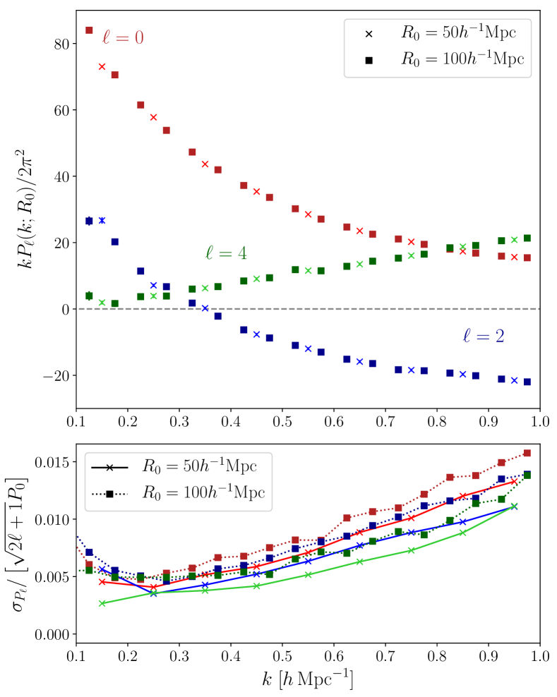
Refer to caption
Figure 5: Upper: Small-scale power spectrum multipoles (upper plot) computed for {0,2,4}024\ell\in\{0,2,4\} for a single QPM mock using the configuration-space power spectrum estimator (Eq. 3.3). We display results counting pairs of particles up to truncation radii of R0=50h1Mpcsubscript𝑅050superscript1MpcR_{0}=50h^{-1}\mathrm{Mpc} and 100h1Mpc100superscript1Mpc100h^{-1}\mathrm{Mpc} in crosses and squares using the linear bins of Δk=0.1hMpc1Δ𝑘0.1superscriptMpc1\Delta k=0.1h\,\mathrm{Mpc}^{-1} and 0.05hMpc10.05superscriptMpc10.05h\,\mathrm{Mpc}^{-1} respectively to minimize cross-talk between bins. We note that the quadrupole spectrum becomes negative for k0.3hMpc1greater-than-or-equivalent-to𝑘0.3superscriptMpc1k\gtrsim 0.3h\,\mathrm{Mpc}^{-1} due to the Finger of God (FoG) effect. We caution that, although the two datasets appear highly consistent here, the error from truncation at R0=50h1Mpcsubscript𝑅050superscript1MpcR_{0}=50h^{-1}\mathrm{Mpc} swamps the statistical error on small scales (cf. Fig. 6). Lower: Standard deviations of the above P(k)subscript𝑃𝑘P_{\ell}(k) measurements for both truncation radii, computed from the variance of 200 QPM mock power spectrum measurements. These are rescaled by the expected ideal isotropic power spectrum scaling of σP(k)2+1P0(k)proportional-tosubscript𝜎subscript𝑃𝑘21subscript𝑃0𝑘\sigma_{P_{\ell}}(k)\propto\sqrt{2\ell+1}P_{0}(k) and are not normalized by Nmockssubscript𝑁mocks\sqrt{N_{\mathrm{mocks}}}, i.e. they represent the error on a single survey measurement. The variances decrease slightly with R0subscript𝑅0R_{0} due to the greater binning width, since this includes more k𝑘k-modes (which are uncorrelated in the Gaussian limit) and leads to greater cancellation between the two D(kr)subscript𝐷𝑘𝑟D_{\ell}(kr) kernels (Eq. A.8).
Refer to caption
Figure 6: Difference between measured QPM power spectrum multipoles (as in Fig. 6) using pair separation truncation radii of R0=50h1Mpcsubscript𝑅050superscript1MpcR_{0}=50h^{-1}\mathrm{Mpc} and R0=100h1Mpcsubscript𝑅0100superscript1MpcR_{0}=100h^{-1}\mathrm{Mpc} in units of the power spectrum error σP(k)subscript𝜎subscript𝑃𝑘\sigma_{P_{\ell}}(k) for R0=100h1Mpcsubscript𝑅0100superscript1MpcR_{0}=100h^{-1}\mathrm{Mpc}. Both datasets are computed using linear k𝑘k-space binning of Δk=0.05hMpc1Δ𝑘0.05superscriptMpc1\Delta k=0.05h\,\mathrm{Mpc}^{-1} (indicated by horizontal error bars) to allow comparison and vertical error bars show the variances across 100 QPM mocks. A slight horizontal offset between multipoles is included for visualization and both plots show the same results but with different k𝑘k-ranges and vertical scales. Beyond k0.4hMpc1similar-to𝑘0.4superscriptMpc1k\sim 0.4h\,\mathrm{Mpc}^{-1} the errors arising from the truncation radius become negligible compared to the statistical errors, with the difference consistent with zero. This is of a similar form to the idealized power ratios of Fig. 2, but we here elect to plot only the difference in power spectra to avoid large deviations from unity when P2(k)0subscript𝑃2𝑘0P_{2}(k)\approx 0, due the the FoG effect. The differences between datasets are expected to arise due to the convolution of the true power with Fourier-space pair-separation windows, W~(k;R0)~𝑊𝑘subscript𝑅0\widetilde{W}(k;R_{0}), of different widths.

Fig. 6 shows the small-scale power spectrum multipoles for the first QPM mock, as well as fractional errors obtained from 200 independent mocks for both aforementioned truncation radii. We note excellent agreement between the two datasets, which is explored further in Fig. 6. The monopole is seen to decrease to small levels with increasing k𝑘k as expected, and we do not find any evidence for a shot-noise plateau (which would give a positive linear asymptote in kP0(k)𝑘subscript𝑃0𝑘kP_{0}(k) for large k𝑘k), as discussed in Sec. 2.4. In addition, the monopole is measured to extremely high precision, at the sub-percent level for much of the range of k𝑘k, with the error bars in the top plot being too small to see. We note that the quadrupole becomes negative for k0.3hMpc1greater-than-or-equivalent-to𝑘0.3superscriptMpc1k\gtrsim 0.3h\,\mathrm{Mpc}^{-1}, which is a result of the FoG effect which dominates at high k𝑘k. FoG has the effect of convolving the true power spectrum with a smoothing kernel along the LoS, which boosts the ksubscript𝑘parallel-tok_{\parallel} power, giving the opposite effect to the Kaiser phenomenon, hence leading to P2(k)<0subscript𝑃2𝑘0P_{2}(k)<0. In this sample, we note the hexadecapole to be small, as expected, with relatively strong constraints obtained on small scales.

In the ideal survey limit with isotropic (and Gaussian) P(𝐤)𝑃𝐤P(\mathbf{k}), the error bars should scale as σP2+1P0(k)proportional-tosubscript𝜎subscript𝑃21subscript𝑃0𝑘\sigma_{P_{\ell}}\propto\sqrt{2\ell+1}P_{0}(k); in the lower part of Fig. 6, the scaling is found to be roughly accurate, though we note larger errors at high-k𝑘k, likely due to the growing importance of higher P(k)subscript𝑃𝑘P_{\ell}(k) multipoles. We also note a small increase in the variance of the power spectrum when moving from R0=50h1Mpcsubscript𝑅050superscript1MpcR_{0}=50h^{-1}\mathrm{Mpc} to R0=100h1Mpcsubscript𝑅0100superscript1MpcR_{0}=100h^{-1}\mathrm{Mpc} which may seem counter-intuitive, since we are utilizing more pairs and obtaining a less well constrained result. This may be rationalized by noting that the bin-spacing (ΔkΔ𝑘\Delta k) is increased by a factor of two between the two datasets (cf. Sec. 6.1) in order to minimize the correlations between neighbouring k𝑘k-bins. Larger ΔkΔ𝑘\Delta k implies an average over a larger range of k𝑘k-modes, which, in the Gaussian limit, are independent, leading to a reduced variance at larger R0subscript𝑅0R_{0}. If the bin-size were kept constant, we would still expect reduced variance, since the diagonal power would be distributed into nearby bins due to the convolution with the pair-separation window W~(k;R0)~𝑊𝑘subscript𝑅0\widetilde{W}(k;R_{0}), whose breadth increases with R0subscript𝑅0R_{0}.

Refer to caption
Figure 7: Ratio of small-scale power spectrum multipoles (a) uncorrected for the survey geometry and (b) corrected, incorporating the survey correction function ΦΦ\Phi (Eq. 2.5), as used in the rest of this paper. We plot the mean and variance of the ratios computed from 20 QPM mocks utilizing a pair-separation truncation radius of R0=100h1Mpcsubscript𝑅0100superscript1MpcR_{0}=100h^{-1}\mathrm{Mpc}. Neither set of multipoles have contributions from shot-noise, since we exclude self-counts in our configuration-space estimator. The uncorrected power monopole P0uncorr(k;R0)superscriptsubscript𝑃0uncorr𝑘subscript𝑅0P_{0}^{\mathrm{\,uncorr}}(k;R_{0}) is equivalent to the FKP power spectrum estimator for large R0subscript𝑅0R_{0} and the higher multipoles are equal to the Bianchi et al. (2015) estimator, except without the Yamamoto et al. (2006) angle approximations (which are negligible at high-k𝑘k). We note significant survey-window-function effects at small k𝑘k, but no significant effects at k0.4hMpc1greater-than-or-equivalent-to𝑘0.4superscriptMpc1k\gtrsim 0.4h\,\mathrm{Mpc}^{-1} except for a slight renormalization (with the ratio tending to 0.954absent0.954\approx 0.954). This is analogous to Fig. 4 except utilizing full simulated data appropriate for BOSS DR12 (and includes additional effects such as the FoG giving different hexadecapole behavior, resulting in the larger deviations between datasets at small k𝑘k).

The effect of R0subscript𝑅0R_{0} on the power spectrum multipoles is considered in Fig. 6, where we consider the difference between P(k;R0)subscript𝑃𝑘subscript𝑅0P_{\ell}(k;R_{0}) at the two values of R0subscript𝑅0R_{0}, normalizing by the statistical error σP(k)subscript𝜎subscript𝑃𝑘\sigma_{P_{\ell}}(k) at the larger R0subscript𝑅0R_{0}. This utilizes Δk=0.05hMpc1Δ𝑘0.05superscriptMpc1\Delta k=0.05h\,\mathrm{Mpc}^{-1} binning for both choices of R0subscript𝑅0R_{0} to allow comparison. The differences between datasets are heuristically similar to those found in the simple forecasts used in Fig. 2, though we now plot the difference in P(k)subscript𝑃𝑘P_{\ell}(k) rather than the ratio, to avoid errors when P2(k)0subscript𝑃2𝑘0P_{2}(k)\approx 0. On large scales, there is significant differences between the datasets which swamp the statistical error, implying that R0=50hMpc1subscript𝑅050superscriptMpc1R_{0}=50h\,\mathrm{Mpc}^{-1} should not be used to measure the k0.3hMpc1less-than-or-similar-to𝑘0.3superscriptMpc1k\lesssim 0.3h\,\mathrm{Mpc}^{-1} power spectrum. For large k𝑘k however, we note excellent agreement between the two datasets, with deviations consistent with zero (given the statistical error) similar to that found in Fig. 2. This clearly demonstrates that R0=50h1Mpcsubscript𝑅050superscript1MpcR_{0}=50h^{-1}\mathrm{Mpc} is a fine (and fast) approximation for measuring very small-scale power. Differences between the simple forecasts and the behavior of Fig. 6 result from the simplifications in the physical model of the former case (which did not include FoG effects) and the binning in k𝑘k-space.

6.2.3 Effects of the Survey-Correction Function ΦΦ\Phi

Using the above estimators, we may assess the dependence of the power spectrum multipoles on the survey-correction function ΦΦ\Phi, analogous to Sec. 4. This (defined as a ratio of RR𝑅𝑅RR pair-counts in Eq. 2.5) was introduced to correct for the non-uniform finite survey geometry and in Fig. 4 was forecasted to significantly effect the mid-k𝑘k power spectrum of higher multipoles. To fully investigate this, we estimate P(k)subscript𝑃𝑘P_{\ell}(k) from QPM mocks with R0=100h1Mpcsubscript𝑅0100superscript1MpcR_{0}=100h^{-1}\mathrm{Mpc} in the same manner as before, but do not include the correction function (i.e. set Φ(r,μ)=1Φ𝑟𝜇1\Phi(r,\mu)=1 for all r𝑟r and μ𝜇\mu). The ratios of these powers are shown in Fig. 7, and we note heuristically similar behavior to Fig. 4, with a large underestimate observed for the hexadecapole, and oscillatory behavior for the lower multipoles whose amplitude falls at large k𝑘k. Here, we note a weaker dependence of the hexadecapole on ΦΦ\Phi than before; this is likely due to the lack of inclusion of FoG effects in the previous forecasting. At large k𝑘k all ratios are seen to converge to 0.95absent0.95\approx 0.95, with the survey-correction function seen to cause an additional slight change in the normalization. Additionally, the error bars show little variation in the uncorrected-to-corrected power ratios with different QPM mocks (except for the small and poorly constrained quadrupole) indicating that this is a true effect of the survey geometry.

6.2.4 Comparison with Simple Models of Anisotropy

For this analysis we will adopt the simple model of Percival & White (2009, Eq. 21) incorporating both Kaiser and FoG effects;

P(k,μ)𝑃𝑘𝜇\displaystyle P(k,\mu) =\displaystyle= b2(1+βμ2)2PNL(k)F(k,μ2)superscript𝑏2superscript1𝛽superscript𝜇22subscript𝑃NL𝑘𝐹𝑘superscript𝜇2\displaystyle b^{2}(1+\beta\mu^{2})^{2}P_{\mathrm{NL}}(k)F(k,\mu^{2}) (6.2)
F(k,μ2)𝐹𝑘superscript𝜇2\displaystyle F(k,\mu^{2}) =\displaystyle= [1+(kμσFoG)2]1superscriptdelimited-[]1superscript𝑘𝜇subscript𝜎FoG21\displaystyle\left[1+(k\mu\sigma_{\mathrm{FoG}})^{2}\right]^{-1}

for (local) bias parameter b𝑏b, Kaiser parameter β=f/b𝛽𝑓𝑏\beta=f/b and FoG velocity dispersion σFoGsubscript𝜎FoG\sigma_{\mathrm{FoG}}. The factor F(k,μ2)𝐹𝑘superscript𝜇2F(k,\mu^{2}) adds Lorentzian FoG effects (Cole et al., 1995; Hamilton, 1998) to the standard Kaiser power spectrum (Kaiser, 1987; Percival & White, 2009), using a non-linear matter power spectrum PNL(k)subscript𝑃NL𝑘P_{\mathrm{NL}}(k), assuming only linear local galaxy bias and no velocity bias. We stress that this is included only to give context and show the approximate impacts of the various RSD effects on the power spectrum. They do not represent our best models, which would incorporate velocity biases and higher order loop corrections. For a redshift-space power spectrum model accurate to k=0.4hMpc1𝑘0.4superscriptMpc1k=0.4h\,\mathrm{Mpc}^{-1}, see Hand et al. (2017).

The non-linear power spectrum is computed via the ‘halofit’ prescription of Mead et al. (2015) using the cosmology {Ωb=0.048,ΩΛ=0.71,h=0.7}formulae-sequencesubscriptΩ𝑏0.048formulae-sequencesubscriptΩΛ0.710.7\{\Omega_{b}=0.048,\Omega_{\Lambda}=0.71,h=0.7\} (matching that used by the White et al. (2014) Quick Particle Mesh (QPM) BOSS DR12 mock catalogs). In the analysis of Gil-Marín et al. (2016a) using the CMASS QPM mocks, the values of b,β,σFoG𝑏𝛽subscript𝜎𝐹𝑜𝐺b,\beta,\sigma_{FoG} were constrained to b=1.74±0.03𝑏plus-or-minus1.740.03b=1.74\pm 0.03, β=0.64±0.05𝛽plus-or-minus0.640.05\beta=0.64\pm 0.05 and σFoG=3.35±0.32subscript𝜎FoGplus-or-minus3.350.32\sigma_{\mathrm{FoG}}=3.35\pm 0.32 in a somewhat more complex model; we adopt these parameters here as a rough estimate. From Eq. 6.2, we may compute the Legendre moments of the model spectrum via the standard integral

P(k)=2+1211𝑑μP(k,μ)L(μ);subscript𝑃𝑘212superscriptsubscript11differential-d𝜇𝑃𝑘𝜇subscript𝐿𝜇\displaystyle P_{\ell}(k)=\frac{2\ell+1}{2}\int_{-1}^{1}d\mu\,P(k,\mu)L_{\ell}(\mu); (6.3)

here we use the full forms tabulated in Lee (2018).
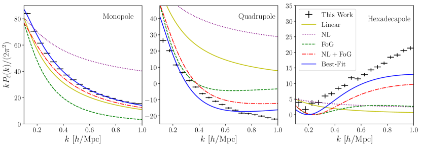
Refer to caption
Figure 8: Comparison of observed (crosses) and model (lines) small-scale power spectrum multipoles (for {0,2,4}024\ell\in\{0,2,4\}) with a variety of simple theoretical RSD models. These models are presented only for context; other models likely provide more accuracy. Observational multipoles are from the QPM results shown in Fig. 6 with R0=100h1Mpcsubscript𝑅0100superscript1MpcR_{0}=100h^{-1}\mathrm{Mpc}, as discussed in Sec. 6.2. The linear power spectrum is computed from CAMB (Lewis & Bridle, 2002) using cosmology appropriate for the QPM mocks at redshift z=0.57𝑧0.57z=0.57. Redshift space distortions (RSD) are added to all models via the Kaiser prescription for (local) bias and β𝛽\beta parameters 1.74 and 0.64 respectively. The ‘NL’ models include a non-linear power spectrum from ‘halofit’ (Mead et al., 2015) at the same redshift and ‘FoG’ models add a Lorentzian Finger of God kernel function (Eq. 6.2) with σFoG=3.35subscript𝜎FoG3.35\sigma_{\mathrm{FoG}}=3.35. All parameters are taken from the DR12 QPM analysis of Gil-Marín et al. (2016a). The ‘best-fit’ model includes both non-linear and FoG effects using a new parameter fit. We note that our simple model does not exactly match that used in the DR12 analysis and is clearly inadequate at higher multipoles (as expected).

In Fig. 8 we plot the R0=100h1Mpcsubscript𝑅0100superscript1MpcR_{0}=100h^{-1}\mathrm{Mpc} power spectrum estimates for a single QPM mock (as above) alongside a variety of models based on Eq. 6.2. These use the aforementioned DR12 analysis parameters, assessing the effects of power spectrum non-linearities and the FoG phenomenon (simply tested by using a linear power spectrum and setting σFoG=0subscript𝜎FoG0\sigma_{\mathrm{FoG}}=0 respectively). For the monopole spectrum we note surprisingly good agreement between the data and the ‘fiducial’ spectrum (simply a linear Kaiser spectrum), with non-linearities and FoG having opposing effects on P0(k)subscript𝑃0𝑘P_{0}(k) which almost cancel. This highlights the use of the higher multipoles in constraining cosmological parameters. In the quadrupole, models without FoG are seen to significantly overestimate the measured power (additionally constraining it to be everywhere positive), with the best approximation given by the inclusion of both FoG and non-linearity. Similar effects are seen for the hexadecapole, with a characteristic minimum in kP4(k)𝑘subscript𝑃4𝑘kP_{4}(k) around 0.2hMpc10.2superscriptMpc10.2h\,\mathrm{Mpc}^{-1} caused by FoG.

Note that the best-fit parameters from the DR12 analysis may not match those required by our somewhat simpler model here; to fully assess how the power spectrum can be fitted by Eq. 6.2, we must optimize for the parameters χ={b,β,σFoG}𝜒𝑏𝛽subscript𝜎FoG\chi=\{b,\beta,\sigma_{\mathrm{FoG}}\}. This is done by minimizing the negative log likelihood

log(χ)=12(𝐏modelT(χ)𝚿QPM𝐏model(χ))+const.𝜒12subscriptsuperscript𝐏𝑇model𝜒subscript𝚿QPMsubscript𝐏model𝜒const\displaystyle-\log\mathcal{L}(\chi)=\frac{1}{2}\left(\mathbf{P}^{T}_{\mathrm{model}}(\chi)\mathbf{\Psi}_{\mathrm{QPM}}\mathbf{P}_{\mathrm{model}}(\chi)\right)+\mathrm{const.} (6.4)

where 𝐏modelsubscript𝐏model\mathbf{P}_{\mathrm{model}} is the (stacked) vector of power spectrum multipoles and 𝚿QPMsubscript𝚿QPM\mathbf{\Psi}_{\mathrm{QPM}} is the QPM precision matrix (see Sec. 6.3) which is independent of the modeling parameters χ𝜒\chi. The errors on the derived parameters χsuperscript𝜒\chi^{*} may be estimated via a standard Fisher forecast giving error on the i𝑖i-th parameter

σχi(𝔽1)iisubscript𝜎subscript𝜒𝑖subscriptsuperscript𝔽1𝑖𝑖\displaystyle\sigma_{\chi_{i}}\approx\sqrt{\left(\mathbb{F}^{-1}\right)_{ii}} (6.5)

for Fisher matrix

𝔽ij=𝐏modelTχi𝚿QPM𝐏modelχj|χ=χsubscript𝔽𝑖𝑗evaluated-atsubscriptsuperscript𝐏𝑇modelsubscript𝜒𝑖subscript𝚿QPMsubscript𝐏modelsubscript𝜒𝑗𝜒superscript𝜒\displaystyle\mathbb{F}_{ij}=\left.\frac{\partial\mathbf{P}^{T}_{\mathrm{model}}}{\partial\chi_{i}}\mathbf{\Psi}_{\mathrm{QPM}}\frac{\partial\mathbf{P}_{\mathrm{model}}}{\partial\chi_{j}}\right|_{\chi=\chi^{*}} (6.6)

which has a simple form since the precision matrix is independent of the model parameters in this case. Using the R0=100h1Mpcsubscript𝑅0100superscript1MpcR_{0}=100h^{-1}\mathrm{Mpc} dataset and the (noisy) QPM precision matrix discussed in Sec. 6.3, we obtain the optimal parameters b=1.95±0.01superscript𝑏plus-or-minus1.950.01b^{*}=1.95\pm 0.01, β=0.48±0.02superscript𝛽plus-or-minus0.480.02\beta^{*}=0.48\pm 0.02 and σFoG=3.54±0.02superscriptsubscript𝜎FoGplus-or-minus3.540.02\sigma_{\mathrm{FoG}}^{*}=3.54\pm 0.02, significantly different from the DR12 analysis due to the simpler model applied here. This model is also shown in Fig. 8 and gives excellent agreement with the monopole power spectrum up to k=1hMpc1𝑘1superscriptMpc1k=1h\,\mathrm{Mpc}^{-1}. The quadrupole spectrum is broadly in agreement up to k0.5hMpc1similar-to𝑘0.5superscriptMpc1k\sim 0.5h\,\mathrm{Mpc}^{-1} and we note an underestimation of the hexadecapole at all scales. This indicates that we require a more sophisticated model to fit the higher-order power multipoles, such as Effective Field Theory. The quoted errors above are very small; this is a result of the very small statistical errors on the monopole and quadrupole. Note that (a) this does not imply that our model is correct, and these are an underestimate since we have not included systematic errors arising from, for example, the pair-separation window function bias, which is non-negligible at small k𝑘k, and (b) the statistical error bars are slightly biased by noise in the precision matrix.

6.3 Covariance Matrix Estimates

The covariance matrix of the above anisotropic power estimates is here computed in two manners; (a) by numerically computing the covariance across the 200 individual QPM power estimates and (b) using the shot-noise rescaled Gaussian prescription of Sec. 5. Whilst it is possible to get far less noisy estimates of the covariance by the latter approach, it is not certain a priori how strongly we are biased by the exclusion of non-Gaussian terms at high-k𝑘k.

6.3.1 QPM Covariance Matrix

Denoting an estimate of the p𝑝p-th multipole power in k𝑘k-space bin a𝑎a from mock i𝑖i as P^p,(i)asubscriptsuperscript^𝑃𝑎𝑝𝑖\hat{P}^{a}_{p,(i)}, the QPM covariance matrix in radial bins a,b𝑎𝑏a,b and Legendre moments p,q𝑝𝑞p,q obtained from Nmocks=200subscript𝑁mocks200N_{\mathrm{mocks}}=200 mocks is defined as

𝐂pqab=1Nmocks1i=1Nmocks[P^p,(i)aP¯pa][P^q,(i)bP¯qb]superscriptsubscript𝐂𝑝𝑞𝑎𝑏1subscript𝑁mocks1superscriptsubscript𝑖1subscript𝑁mocksdelimited-[]subscriptsuperscript^𝑃𝑎𝑝𝑖subscriptsuperscript¯𝑃𝑎𝑝delimited-[]subscriptsuperscript^𝑃𝑏𝑞𝑖subscriptsuperscript¯𝑃𝑏𝑞\displaystyle\mathbf{C}_{pq}^{ab}=\frac{1}{N_{\mathrm{mocks}}-1}\sum_{i=1}^{N_{\mathrm{mocks}}}\left[\hat{P}^{a}_{p,(i)}-\overline{P}^{a}_{p}\right]\left[\hat{P}^{b}_{q,(i)}-\overline{P}^{b}_{q}\right] (6.7)

for power spectrum mean

P¯pa=1Nmocksi=1NmocksP^p,(i)a.subscriptsuperscript¯𝑃𝑎𝑝1subscript𝑁mockssuperscriptsubscript𝑖1subscript𝑁mockssubscriptsuperscript^𝑃𝑎𝑝𝑖\displaystyle\overline{P}^{a}_{p}=\frac{1}{N_{\mathrm{mocks}}}\sum_{i=1}^{N_{\mathrm{mocks}}}\hat{P}^{a}_{p,(i)}. (6.8)

This may be used to find the correlation matrix 𝐑pqabsubscriptsuperscript𝐑𝑎𝑏𝑝𝑞\mathbf{R}^{ab}_{pq} which is defined by

𝐑pqab=𝐂pqab𝐂ppaa𝐂qqbbsuperscriptsubscript𝐑𝑝𝑞𝑎𝑏superscriptsubscript𝐂𝑝𝑞𝑎𝑏superscriptsubscript𝐂𝑝𝑝𝑎𝑎superscriptsubscript𝐂𝑞𝑞𝑏𝑏\displaystyle\mathbf{R}_{pq}^{ab}=\frac{\mathbf{C}_{pq}^{ab}}{\sqrt{\mathbf{C}_{pp}^{aa}\mathbf{C}_{qq}^{bb}}} (6.9)

with unity along the p=q𝑝𝑞p=q, a=b𝑎𝑏a=b leading diagonal by construction. This is shown for the two choice of R0subscript𝑅0R_{0} in Fig. 9, using the Δk=5/R0Δ𝑘5subscript𝑅0\Delta k=5/R_{0} binning as before, to ensure minimal cross-talk between k𝑘k-bins induced by the pair-separation window function. Notably we observe a significant positive correlation between all k𝑘k-bins at the same Legendre multipole especially at larger k𝑘k; this may result from non-Gaussian terms (cf. trispectrum terms discussed in Sec.  6.1), the effects of the non-trivial survey geometry or additional mixing between k𝑘k-bins induced by the pair-separation window W~(k;R0)~𝑊𝑘subscript𝑅0\widetilde{W}(k;R_{0}). In addition, we note small negative correlations between the quadrupole and other multipoles and very weak correlations between the hexadecapole and monopole.
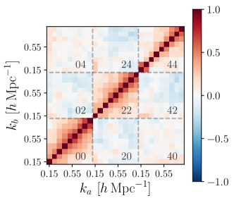
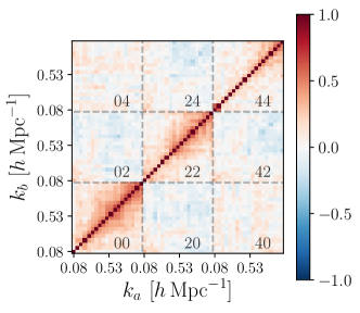
Refer to caption
(a) R0=50h1Mpcsubscript𝑅050superscript1MpcR_{0}=50h^{-1}\mathrm{Mpc}, Δk=0.1hMpc1Δ𝑘0.1superscriptMpc1\Delta k=0.1h\,\mathrm{Mpc}^{-1}
Refer to caption
(b) R0=100h1Mpcsubscript𝑅0100superscript1MpcR_{0}=100h^{-1}\mathrm{Mpc}, Δk=0.05hMpc1Δ𝑘0.05superscriptMpc1\Delta k=0.05h\,\mathrm{Mpc}^{-1}
Figure 9: Correlation matrix for small-scale power spectrum multipoles measured from 200 QPM mocks using the configuration-space power estimator (Eq. 3.3) with pair-counts truncated at two radii R0subscript𝑅0R_{0} (with associated powers shown in Fig. 6). The correlation matrix is defined by Eq. 6.9 and we display all combinations of Legendre multipoles in each (symmetric) figure. The dotted lines demarcate submatrices for different pairs of Legendre multipoles (e.g. (02)02(02) indicates the cross-covariance between =00\ell=0 and =22\ell=2) with a total of 9 (19) radial bins in each for R0=50subscript𝑅050R_{0}=50 (100100100) h1Mpcsuperscript1Mpch^{-1}\mathrm{Mpc}. We note negative correlations with the =22\ell=2 multipoles and significant off-diagonal correlations increasing to larger k𝑘k due to the survey selection function, the pairwise window function and non-Gaussianity.

The precision matrix is formally defined as the inverse of the covariance matrix, yet, in the limit of finite mocks, this introduces a bias to the estimate which causes bias in the derived parameter variances. Assuming Wishart noise (Wishart, 1928), we apply the Hartlap et al. (2007) correction factor to obtain the QPM precision matrix estimate

𝚿pqab=NmocksNbins2Nmocks1(𝐂pqab)1superscriptsubscript𝚿𝑝𝑞𝑎𝑏subscript𝑁mockssubscript𝑁bins2subscript𝑁mocks1superscriptsuperscriptsubscript𝐂𝑝𝑞𝑎𝑏1\displaystyle\mathbf{\Psi}_{pq}^{ab}=\frac{N_{\mathrm{mocks}}-N_{\mathrm{bins}}-2}{N_{\mathrm{mocks}}-1}\left(\mathbf{C}_{pq}^{ab}\right)^{-1} (6.10)

where Nbinssubscript𝑁binsN_{\mathrm{bins}} is the total number of bins across all multipoles. This is shown in Fig. 10 in the same fashion as above, and has an approximately tridiagonal form, with strong positive diagonal contributions for p=q𝑝𝑞p=q and significant negative next-to-diagonal terms but little additional power. As expected, the precision matrix elements are largest for the monopole as this is known most precisely (cf. Fig. 6). This precision matrix may be used to compute Fisher forecasts, as in Sec. 6.2.4.
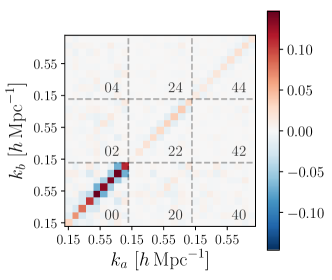
Refer to caption
(a) R0=50h1Mpcsubscript𝑅050superscript1MpcR_{0}=50h^{-1}\mathrm{Mpc}
Refer to caption
(b) R0=100h1Mpcsubscript𝑅0100superscript1MpcR_{0}=100h^{-1}\mathrm{Mpc}
Figure 10: Sample QPM precision matrices 𝚿pqabsuperscriptsubscript𝚿𝑝𝑞𝑎𝑏\mathbf{\Psi}_{pq}^{ab} (defined by Eq. 6.10) for the two covariance matrices shown in Fig. 9. These are divided by k1k2subscript𝑘1subscript𝑘2k_{1}k_{2} for ease of visualization.These use 200 mocks as before and we note a strong diagonal and next-to-diagonal term for p=q𝑝𝑞p=q but little other power. These can be used in Fisher forecasting to find the constraints on derived model parameters such as RSD parameters.

6.3.2 Theoretical Covariance Matrix

To compute the theoretical rescaled-Gaussian covariances, we adopt the implementation described in Sec. 5.2, first computing the weighting functions {Ωpq2(u),Ωpq3(u1,u2),Ωpq4(u1,u2)}superscriptsubscriptΩ𝑝𝑞2𝑢superscriptsubscriptΩ𝑝𝑞3subscript𝑢1subscript𝑢2superscriptsubscriptΩ𝑝𝑞4subscript𝑢1subscript𝑢2\left\{{}^{2}\Omega_{pq}(u),{}^{3}\Omega_{pq}(u_{1},u_{2}),{}^{4}\Omega_{pq}(u_{1},u_{2})\right\} across the domain [0,R0]0subscript𝑅0[0,R_{0}]. This is performed using a modified version of the RascalC as previously noted, and we produce estimates of the ΩpqsubscriptΩ𝑝𝑞\Omega_{pq} functions (Eqs. 5.11 & 5.13) in 1000 radial bins with Δr=0.1h1MpcΔ𝑟0.1superscript1Mpc\Delta r=0.1h^{-1}\mathrm{Mpc} regularly spaced in [0,R0]0subscript𝑅0[0,R_{0}], computed for 1013similar-toabsentsuperscript1013\sim 10^{13} quads of particles in 200similar-toabsent200\sim 200 CPU-hours. The two-, three- and four-point weighting functions for all combinations of Legendre moments (p,q)𝑝𝑞(p,q) are shown in Fig. 11 (and we note that these appear to be smooth, with Ωpq(u)0subscriptΩ𝑝𝑞𝑢0\Omega_{pq}(u)\rightarrow 0 as uR0𝑢subscript𝑅0u\rightarrow R_{0} for all functions, as expected. Notably, the ΩΩ\Omega functions are large and positive for p=q𝑝𝑞p=q elements, with negative terms arising for combinations of the quadrupole with other multipoles.
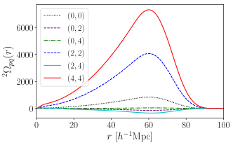
Refer to caption
(a) Two-point, Ωpq2(r)superscriptsubscriptΩ𝑝𝑞2𝑟{}^{2}\Omega_{pq}(r)
Refer to caption
(b) Three-point, Ωpq3(r1,r2)superscriptsubscriptΩ𝑝𝑞3subscript𝑟1subscript𝑟2{}^{3}\Omega_{pq}(r_{1},r_{2})
Refer to caption
(c) Four-point, Ωpq4(r1,r2)superscriptsubscriptΩ𝑝𝑞4subscript𝑟1subscript𝑟2{}^{4}\Omega_{pq}(r_{1},r_{2})
Figure 11: Gaussian covariance unnormalized probability density functions (PDFs) for the two-, three- and four-point power spectrum covariance matrices at R0=100h1Mpcsubscript𝑅0100superscript1MpcR_{0}=100h^{-1}\mathrm{Mpc}, as defined in Eqs. 5.11 & 5.13, here using Δk=0.1h1MpcΔ𝑘0.1superscript1Mpc\Delta k=0.1h^{-1}\mathrm{Mpc} radial bins. These are used to compute the expected rescaled-Gaussian power spectrum covariance matrices via Eqs. 5.10 & 5.12, shown in Fig. 11. Physically these are the distribution functions of pair-wise separations, weighted by the survey correction functions, pair-separation windows, number densities and correlation functions, such that the covariance matrices can be defined as a integral over these with a k𝑘k-dependent kernel. The two-point integral is shown in the leftmost plot, which is diagonal for each set of Legendre indices with lines labelled by (p,q)𝑝𝑞(p,q) representing the Ωpq2(r)superscriptsubscriptΩ𝑝𝑞2𝑟{}^{2}\Omega_{pq}(r) function. The Ωpq3superscriptsubscriptΩ𝑝𝑞3{}^{3}\Omega_{pq} and Ωpq4superscriptsubscriptΩ𝑝𝑞4{}^{4}\Omega_{pq} matrices are plotted in the same style as Figs. 9 & 10 except in configuration-space.

These are combined via Eqs. 5.10 & 5.12 to form the full Gaussian covariance matrix components, which are displayed in Fig. 12. Since the ΩpqsubscriptΩ𝑝𝑞\Omega_{pq} matrices are well converged, the integrals over r𝑟r are approximated simply by summations; for less well converged matrices one could fit ΩpqsubscriptΩ𝑝𝑞\Omega_{pq} to smooth functions before performing the k𝑘k-space kernel weighted integration. Although the four-point terms are dominant on large scales (small k𝑘k), the two- and three-point covariance matrix terms are the leading contributions at large k𝑘k. The latter terms are sourced by shot-noise contractions (appearing in the covariances not the power spectra) which are expected to dominate on small-scales when the power is subdominant. In addition, we note significant off-diagonal power in the two-point matrix and (at small k𝑘k) the higher-point matrices. Since these do not include non-Gaussian terms, this is expected to arise from k𝑘k-bin mixing or survey geometry effects, not from any intrinsic 4PCF terms.
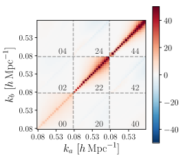
Refer to caption
(a) Two-point, Cpqab2×kakbsuperscriptsuperscriptsubscript𝐶𝑝𝑞𝑎𝑏2subscript𝑘𝑎subscript𝑘𝑏{}^{2}C_{pq}^{ab}\times k_{a}k_{b}
Refer to caption
(b) Three-point, Cpqab3×kakbsuperscriptsuperscriptsubscript𝐶𝑝𝑞𝑎𝑏3subscript𝑘𝑎subscript𝑘𝑏{}^{3}C_{pq}^{ab}\times k_{a}k_{b}
Refer to caption
(c) Four-point, Cpqab4×kakbsuperscriptsuperscriptsubscript𝐶𝑝𝑞𝑎𝑏4subscript𝑘𝑎subscript𝑘𝑏{}^{4}C_{pq}^{ab}\times k_{a}k_{b}
Figure 12: Two-, three- and four-point theoretical Gaussian covariance matrices, as defined in Eq. 5.4, here using R0=100h1Mpcsubscript𝑅0100superscript1MpcR_{0}=100h^{-1}\mathrm{Mpc} and 19 k𝑘k-bins linearly spaced in [0.15,1]0.151[0.15,1] (matching that of Fig. 9). Matrices are multiplied by kakbsubscript𝑘𝑎subscript𝑘𝑏k_{a}k_{b} for visibility. The individual terms are given by integrals of the 2PCF ξ𝜉\xi and kernel functions Apa(r)subscriptsuperscript𝐴𝑎𝑝𝑟A^{a}_{p}(r) over two to four copies of the survey. Two- and three-point terms arise from shot-noise contributions to the covariance. Here, they are computed from integrating k𝑘k-space kernel functions over the smooth distributions functions of Fig. 11, according to Eqs. 5.10 & 5.12. These may be summed via Eq. 5.5 to form a full estimate of the covariance matrix, with shot-noise rescaling parameter α𝛼\alpha encapsulating some non-Gaussianity. The three- and four-point covariance terms are seen to dominate at small k𝑘k, with largest contributions on very small scales from the two-point term. We note clear off-diagonal terms here resulting from the non-uniform survey geometry and the pair-separation window function.

The full theoretical covariance matrix is found from Eq. 5.5, with a shot-noise rescaling parameter α𝛼\alpha allowing inclusion of some non-Gaussianity. Here the parameter is constrained by fitting the theoretical to QPM covariance matrix; one could also compute this from a single survey via jackknife approaches (cf.  O’Connell & Eisenstein, 2019; Philcox et al., 2019). The two matrices are compared via the 1subscript1\mathcal{L}_{1} likelihood

log1(α)=2DKL(Ψ(α),𝐂QPM)=trace[Ψ(α)𝐂QPM]logdet𝐂QPMlogdetΨ(α)Nbinssubscript1𝛼2subscript𝐷𝐾𝐿Ψ𝛼subscript𝐂QPMtraceΨ𝛼subscript𝐂QPMsubscript𝐂QPMΨ𝛼subscript𝑁bins\displaystyle-\log\mathcal{L}_{1}(\alpha)=2D_{KL}\left(\Psi(\alpha),\mathbf{C}_{\mathrm{QPM}}\right)=\operatorname{trace}[\Psi(\alpha)\mathbf{C}_{\mathrm{QPM}}]-\log\det\mathbf{C}_{\mathrm{QPM}}-\log\det\Psi(\alpha)-N_{\mathrm{bins}} (6.11)

where DKLsubscript𝐷𝐾𝐿D_{KL} is the Kullback-Leibler (KL) divergence (Kullback & Leibler, 1951). Note that this depends on the theoretical precision matrix; since this is computed at low noise, we can assume Ψ(α)=C1(α)Ψ𝛼superscript𝐶1𝛼\Psi(\alpha)=C^{-1}(\alpha) with minimal error. Numerical minimization of this likelihood gives an optimal shot-noise rescaling parameter α=1.13superscript𝛼1.13\alpha^{*}=1.13.

6.3.3 Covariance Matrix Comparison

A simple method by which to compare the QPM and theory covariance matrices is the KL divergence used in Eq. 6.11. As shown in Philcox et al. (2019, Appendix D), the expected KL divergence between the two matrices is approximately given by

DKL(Ψ,𝐂QPM)Nbins(Nbins+1)4Nmocksdelimited-⟨⟩subscript𝐷𝐾𝐿Ψsubscript𝐂QPMsubscript𝑁binssubscript𝑁bins14subscript𝑁mocks\displaystyle\langle{D_{KL}(\Psi,\mathbf{C}_{\mathrm{QPM}})\rangle}\approx\frac{N_{\mathrm{bins}}(N_{\mathrm{bins}}+1)}{4N_{\mathrm{mocks}}} (6.12)

(assuming a smooth precision matrix). Here, the true KL divergence is found to be 5.35.35.3 compared to an expected value of 4.34.34.3. Since this only becomes exact in the limit of NmocksNbinsmuch-greater-thansubscript𝑁mockssubscript𝑁binsN_{\mathrm{mocks}}\gg N_{\mathrm{bins}} we conclude that the matrices appear broadly consistent at this level.
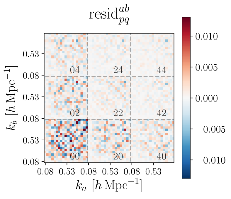
Refer to caption
Figure 13: Residual matrix between the QPM precision matrix (Fig. 10) and the theoretical precision matrix computed from the shot-noise-rescaled Gaussian terms of Fig. 12, i.e. Eq. 6.13, using shot-noise rescaling α=1.13𝛼1.13\alpha=1.13. The residual is normalized by kakbsubscript𝑘𝑎subscript𝑘𝑏k_{a}k_{b} for visualization and uses R0=100h1Mpcsubscript𝑅0100superscript1MpcR_{0}=100h^{-1}\mathrm{Mpc} and Δk=0.05hMpc1Δ𝑘0.05superscriptMpc1\Delta k=0.05h\,\mathrm{Mpc}^{-1}, displaying all cross-covariances for {0,2,4}024\ell\in\{0,2,4\} as before. The residual matrix appears mostly consistent with noise here. A more obvious comparison of these covariances is presented in Fig. 14.
Refer to caption
Figure 14: Discriminant matrix encapsulating the differences between theory (Fig. 12 with α=1.13𝛼1.13\alpha=1.13) and simulation (Figs. 9 & 10) covariance matrices for QPM mocks, as defined in Eq. 6.14. For identical covariance matrices, the discriminant matrix will be equal to zero in the limit of zero noise; systematic differences from zero indicate biases in the theoretical model. We note no obvious biases in the monopole matrices, with a slight positive bias in the two-point matrix at small k𝑘k and a small diagonal bias at large k𝑘k in the p=q=4𝑝𝑞4p=q=4 matrix. This could be removed using an improved model for non-Gaussianity in the covariance matrix, for example hierarchical models.

A more graphic method is to consider the matrix residual, given by the rescaled difference between the precision matrices;

residpqab=(Ψ(α)𝚿QPM)pqabkakb.subscriptsuperscriptresid𝑎𝑏𝑝𝑞subscriptsuperscriptΨsuperscript𝛼subscript𝚿QPM𝑎𝑏𝑝𝑞subscript𝑘𝑎subscript𝑘𝑏\displaystyle\mathrm{resid}^{ab}_{pq}=\frac{\left(\Psi(\alpha^{*})-\mathbf{\Psi}_{\mathrm{QPM}}\right)^{ab}_{pq}}{k_{a}k_{b}}. (6.13)

Any significant departures of this from zero indicate systematic differences between the matrices. Note that we here compare the precision matrices rather than the covariances since these are more relevant cosmologically. Fig. 14 displays this matrix and the behavior appears largely consistent with noise, with larger fluctuations observed for the =00\ell=0 multipoles as expected, since these include the dominant power in the precision matrices. We note a slight underestimation of the p=q=4𝑝𝑞4p=q=4 matrix diagonal in the theoretical matrix which is likely due to the lack of inclusion of non-Gaussianity in the model. At this level of noise, it is difficult to see any major systematic differences between matrices.

An additional test uses the ‘discriminant’ matrix which we define as

discpqab=(Ψ(α)T𝐂QPMΨ(α)𝕀)pqabsubscriptsuperscriptdisc𝑎𝑏𝑝𝑞subscriptsuperscriptsuperscriptΨsuperscript𝛼𝑇subscript𝐂QPMΨsuperscript𝛼𝕀𝑎𝑏𝑝𝑞\displaystyle\mathrm{disc}^{ab}_{pq}=\left(\sqrt{\Psi(\alpha^{*})}^{T}\mathbf{C}_{\mathrm{QPM}}\sqrt{\Psi(\alpha^{*})}-\mathbb{I}\right)^{ab}_{pq} (6.14)

where Ψ(α)Ψsuperscript𝛼\sqrt{\Psi(\alpha^{*})} indicates the Cholesky factorization of the theoretical precision matrix. For identical covariance matrices in the zero-noise limit, we expect Ψ(α)=𝐂QPM1Ψsuperscript𝛼superscriptsubscript𝐂QPM1\Psi(\alpha^{*})=\mathbf{C}_{\mathrm{QPM}}^{-1} thus discpqab=𝟎subscriptsuperscriptdisc𝑎𝑏𝑝𝑞0\mathrm{disc}^{ab}_{pq}=\mathbf{0}. Any systematic deviations from zero indicate shortcomings in our theoretical matrices. This is plotted in Fig. 14 for the same matrices as before, and we note no significant departures from zero for the monopole covariances implying that these terms are well estimated. For the p=q=2𝑝𝑞2p=q=2 quadrupole autocovariance there is a clear bias for small k𝑘k, indicating that our model is insufficient there. This likely arises from non-Gaussianity since the non-Gaussian terms only appear in the three- and four-point theoretical covariance matrices which dominate at small k𝑘k. We additionally note a slight negative diagonal bias for p=q=4𝑝𝑞4p=q=4. Overall, we note remarkable agreement between the rescaled-Gaussian theory and QPM mock covariance matrices for most monopoles, with the exception of the k0.3hMpc1less-than-or-similar-to𝑘0.3superscriptMpc1k\lesssim 0.3h\,\mathrm{Mpc}^{-1} quadrupole autocovariance. Increasing the model complexity is expected to further improve the fit; a simple approach to this is via hierarchical 3PCF and 4PCF models (e.g. Peebles & Groth, 1975; Groth & Peebles, 1977) that add an additional free hierarchical parameter Q𝑄Q which could be fit to mocks or jackknifes.

7 Bispectrum Estimators

We conclude by outlining estimators for the isotropic bispectrum in a similar fashion to the above, with computation possible via weighted triple-counting. We defer considerations of the bispectrum covariance and power spectrum - bispectrum cross-covariance to future work, although note that this may be derived as for the power spectrum and estimated using small modifications to the 3PCF covariance algorithm of Philcox & Eisenstein (2019).

7.1 Idealized Estimator

We start with the definition of the bispectrum as the transform of the three-point correlation function (3PCF) ζ𝜁\zeta;

δ(D)(𝐤1+𝐤2+𝐤3)B(𝐤1,𝐤2,𝐤3)B(𝐤1,𝐤2)=d3𝐱1d3𝐱2ei[𝐤1𝐱1+𝐤2𝐱2]ζ(𝐱1,𝐱2)superscript𝛿𝐷subscript𝐤1subscript𝐤2subscript𝐤3𝐵subscript𝐤1subscript𝐤2subscript𝐤3𝐵subscript𝐤1subscript𝐤2superscript𝑑3subscript𝐱1superscript𝑑3subscript𝐱2superscript𝑒𝑖delimited-[]subscript𝐤1subscript𝐱1subscript𝐤2subscript𝐱2𝜁subscript𝐱1subscript𝐱2\displaystyle\delta^{(D)}(\mathbf{k}_{1}+\mathbf{k}_{2}+\mathbf{k}_{3})\,B(\mathbf{k}_{1},\mathbf{k}_{2},\mathbf{k}_{3})\equiv B(\mathbf{k}_{1},\mathbf{k}_{2})=\int d^{3}\mathbf{x}_{1}\,d^{3}\mathbf{x}_{2}\,e^{i[\mathbf{k}_{1}\cdot\mathbf{x}_{1}+\mathbf{k}_{2}\cdot\mathbf{x}_{2}]}\zeta(\mathbf{x}_{1},\mathbf{x}_{2}) (7.1)

for Dirac delta function δ(D)superscript𝛿𝐷\delta^{(D)} enforcing the triangle condition on the wavevector 𝐤isubscript𝐤𝑖\mathbf{k}_{i}. On the right hand side, this condition has been used, and we write the 3PCF as a function of two triangle sides, 𝐱1subscript𝐱1\mathbf{x}_{1} and 𝐱2subscript𝐱2\mathbf{x}_{2}. Using the Szapudi & Szalay (1998) 3PCF estimator, we may proceed analogously to the power spectrum case, writing

B(𝐤1,𝐤2)=d3𝐱1d3𝐱2ei[𝐤1𝐱1+𝐤2𝐱2]NNN(𝐱1,𝐱2)RRR(𝐱1,𝐱2)𝐵subscript𝐤1subscript𝐤2superscript𝑑3subscript𝐱1superscript𝑑3subscript𝐱2superscript𝑒𝑖delimited-[]subscript𝐤1subscript𝐱1subscript𝐤2subscript𝐱2𝑁𝑁𝑁subscript𝐱1subscript𝐱2𝑅𝑅𝑅subscript𝐱1subscript𝐱2\displaystyle B(\mathbf{k}_{1},\mathbf{k}_{2})=\int d^{3}\mathbf{x}_{1}\,d^{3}\mathbf{x}_{2}\,e^{i[\mathbf{k}_{1}\cdot\mathbf{x}_{1}+\mathbf{k}_{2}\cdot\mathbf{x}_{2}]}\frac{NNN(\mathbf{x}_{1},\mathbf{x}_{2})}{RRR(\mathbf{x}_{1},\mathbf{x}_{2})} (7.2)

for triple-counts NNN𝑁𝑁𝑁NNN and RRR𝑅𝑅𝑅RRR. These are defined as

RRR(𝐱1,𝐱2)𝑅𝑅𝑅subscript𝐱1subscript𝐱2\displaystyle RRR(\mathbf{x}_{1},\mathbf{x}_{2}) \displaystyle\equiv {i=13d3𝐫in(𝐫i)w(𝐫i)}[δ(D)(𝐱1(𝐫1𝐫3))δ(D)(𝐱2(𝐫2𝐫3))+(5 perms. of {𝐫1,𝐫2,𝐫3})]superscriptsubscriptproduct𝑖13superscript𝑑3subscript𝐫𝑖𝑛subscript𝐫𝑖𝑤subscript𝐫𝑖delimited-[]superscript𝛿𝐷subscript𝐱1subscript𝐫1subscript𝐫3superscript𝛿𝐷subscript𝐱2subscript𝐫2subscript𝐫35 perms. of {𝐫1,𝐫2,𝐫3}\displaystyle\int\left\{\prod_{i=1}^{3}d^{3}\mathbf{r}_{i}\,n(\mathbf{r}_{i})w(\mathbf{r}_{i})\right\}\left[\delta^{(D)}(\mathbf{x}_{1}-(\mathbf{r}_{1}-\mathbf{r}_{3}))\delta^{(D)}(\mathbf{x}_{2}-(\mathbf{r}_{2}-\mathbf{r}_{3}))+\left(\text{5 perms. of $\{\mathbf{r}_{1},\mathbf{r}_{2},\mathbf{r}_{3}\}$}\right)\right] (7.3)
NNN(𝐱1,𝐱2)𝑁𝑁𝑁subscript𝐱1subscript𝐱2\displaystyle NNN(\mathbf{x}_{1},\mathbf{x}_{2}) \displaystyle\equiv {i=13d3𝐫in(𝐫i)w(𝐫i)δ(𝐫i)}[δ(D)(𝐱1(𝐫1𝐫3))δ(D)(𝐱2(𝐫2𝐫3))+(5 perms. of {𝐫1,𝐫2,𝐫3})].superscriptsubscriptproduct𝑖13superscript𝑑3subscript𝐫𝑖𝑛subscript𝐫𝑖𝑤subscript𝐫𝑖𝛿subscript𝐫𝑖delimited-[]superscript𝛿𝐷subscript𝐱1subscript𝐫1subscript𝐫3superscript𝛿𝐷subscript𝐱2subscript𝐫2subscript𝐫35 perms. of {𝐫1,𝐫2,𝐫3}\displaystyle\int\left\{\prod_{i=1}^{3}d^{3}\mathbf{r}_{i}\,n(\mathbf{r}_{i})w(\mathbf{r}_{i})\delta(\mathbf{r}_{i})\right\}\left[\delta^{(D)}(\mathbf{x}_{1}-(\mathbf{r}_{1}-\mathbf{r}_{3}))\delta^{(D)}(\mathbf{x}_{2}-(\mathbf{r}_{2}-\mathbf{r}_{3}))+\left(\text{5 perms. of $\{\mathbf{r}_{1},\mathbf{r}_{2},\mathbf{r}_{3}\}$}\right)\right].

For thin k𝑘k-space bins (a,b)𝑎𝑏(a,b) with center (𝐱a,𝐱b)subscript𝐱𝑎subscript𝐱𝑏(\mathbf{x}_{a},\mathbf{x}_{b}) and size δ𝐱𝛿𝐱\delta\mathbf{x}, in the ideal survey limit (with uniform n𝑛n, w𝑤w) we obtain;

RRRab𝑅𝑅superscript𝑅𝑎𝑏\displaystyle RRR^{ab} \displaystyle\approx RRR(𝐱a,𝐱b)(δ𝐱)2=(nw)3d3𝐫1d3𝐫2d3𝐫3[Θa(𝐫1𝐫3)Θb(𝐫2𝐫3)+(5 perms.)]𝑅𝑅𝑅subscript𝐱𝑎subscript𝐱𝑏superscript𝛿𝐱2superscript𝑛𝑤3superscript𝑑3subscript𝐫1superscript𝑑3subscript𝐫2superscript𝑑3subscript𝐫3delimited-[]superscriptΘ𝑎subscript𝐫1subscript𝐫3superscriptΘ𝑏subscript𝐫2subscript𝐫35 perms.\displaystyle RRR(\mathbf{x}_{a},\mathbf{x}_{b})\left(\delta\mathbf{x}\right)^{2}=(nw)^{3}\int d^{3}\mathbf{r}_{1}\,d^{3}\mathbf{r}_{2}\,d^{3}\mathbf{r}_{3}\,\left[\Theta^{a}(\mathbf{r}_{1}-\mathbf{r}_{3})\Theta^{b}(\mathbf{r}_{2}-\mathbf{r}_{3})+\left(\text{5 perms.}\right)\right]
=\displaystyle= 6V(nw)3(δ𝐱)26𝑉superscript𝑛𝑤3superscript𝛿𝐱2\displaystyle 6V(nw)^{3}\left(\delta\mathbf{x}\right)^{2}

using binning functions Θc(𝐱)superscriptΘ𝑐𝐱\Theta^{c}(\mathbf{x}) which are unity if 𝐱𝐱\mathbf{x} is in bin c𝑐c and zero else. As before, this permits the modeling of a general RRR𝑅𝑅𝑅RRR count as

RRR(𝐱1,𝐱2)=6V(nw)3¯Φ(𝐱1,𝐱2)𝑅𝑅𝑅subscript𝐱1subscript𝐱26𝑉¯superscript𝑛𝑤3Φsubscript𝐱1subscript𝐱2\displaystyle RRR(\mathbf{x}_{1},\mathbf{x}_{2})=\frac{6V\overline{(nw)^{3}}}{\Phi(\mathbf{x}_{1},\mathbf{x}_{2})} (7.5)

for survey correction factor Φ(𝐱1,𝐱2)Φsubscript𝐱1subscript𝐱2\Phi(\mathbf{x}_{1},\mathbf{x}_{2}) now depending on three points in space (parametrized by two separation vectors). Analogous to the power spectrum definition, we may write the bispectrum as

B(𝐤1,𝐤2)𝐵subscript𝐤1subscript𝐤2\displaystyle B(\mathbf{k}_{1},\mathbf{k}_{2}) =\displaystyle= 16V(nw)3¯{i=13d3𝐫in(𝐫i)w(𝐫i)δ(𝐫i)}[Φ(𝐫1𝐫3,𝐫2𝐫3)ei[𝐤1(𝐫1𝐫3)+𝐤2(𝐫2𝐫3)]+(5 perms.)]16𝑉¯superscript𝑛𝑤3superscriptsubscriptproduct𝑖13superscript𝑑3subscript𝐫𝑖𝑛subscript𝐫𝑖𝑤subscript𝐫𝑖𝛿subscript𝐫𝑖delimited-[]Φsubscript𝐫1subscript𝐫3subscript𝐫2subscript𝐫3superscript𝑒𝑖delimited-[]subscript𝐤1subscript𝐫1subscript𝐫3subscript𝐤2subscript𝐫2subscript𝐫35 perms.\displaystyle\frac{1}{6V\overline{(nw)^{3}}}\int\left\{\prod_{i=1}^{3}d^{3}\mathbf{r}_{i}\,n(\mathbf{r}_{i})w(\mathbf{r}_{i})\delta(\mathbf{r}_{i})\right\}\left[\Phi(\mathbf{r}_{1}-\mathbf{r}_{3},\mathbf{r}_{2}-\mathbf{r}_{3})e^{i\left[\mathbf{k}_{1}\cdot(\mathbf{r}_{1}-\mathbf{r}_{3})+\mathbf{k}_{2}\cdot(\mathbf{r}_{2}-\mathbf{r}_{3})\right]}+\left(\text{5 perms.}\right)\right]
=\displaystyle= 1V(nw)3¯{i=13d3𝐫in(𝐫i)w(𝐫i)δ(𝐫i)}Φ(𝐫1𝐫3,𝐫2𝐫3)ei[𝐤1(𝐫1𝐫3)+𝐤2(𝐫2𝐫3)]1𝑉¯superscript𝑛𝑤3superscriptsubscriptproduct𝑖13superscript𝑑3subscript𝐫𝑖𝑛subscript𝐫𝑖𝑤subscript𝐫𝑖𝛿subscript𝐫𝑖Φsubscript𝐫1subscript𝐫3subscript𝐫2subscript𝐫3superscript𝑒𝑖delimited-[]subscript𝐤1subscript𝐫1subscript𝐫3subscript𝐤2subscript𝐫2subscript𝐫3\displaystyle\frac{1}{V\overline{(nw)^{3}}}\int\left\{\prod_{i=1}^{3}d^{3}\mathbf{r}_{i}\,n(\mathbf{r}_{i})w(\mathbf{r}_{i})\delta(\mathbf{r}_{i})\right\}\Phi(\mathbf{r}_{1}-\mathbf{r}_{3},\mathbf{r}_{2}-\mathbf{r}_{3})e^{i\left[\mathbf{k}_{1}\cdot(\mathbf{r}_{1}-\mathbf{r}_{3})+\mathbf{k}_{2}\cdot(\mathbf{r}_{2}-\mathbf{r}_{3})\right]}

integrating over the Dirac delta functions in the NNN𝑁𝑁𝑁NNN definition to set 𝐱1,𝐱2subscript𝐱1subscript𝐱2\mathbf{x}_{1},\mathbf{x}_{2} in ΦΦ\Phi, and noting that the second line follows since Φ(𝐫i𝐫j,𝐫i𝐫k)Φsubscript𝐫𝑖subscript𝐫𝑗subscript𝐫𝑖subscript𝐫𝑘\Phi(\mathbf{r}_{i}-\mathbf{r}_{j},\mathbf{r}_{i}-\mathbf{r}_{k}) is symmetric under any permutation of {i,j,k}𝑖𝑗𝑘\{i,j,k\}. Here we note that, in the limit of an ideal survey, where Φ=1Φ1\Phi=1 everywhere, this is identical to the standard estimator, which can be written as

δ(D)(𝐤1+𝐤2+𝐤3)B(𝐤1,𝐤2)superscript𝛿𝐷subscript𝐤1subscript𝐤2subscript𝐤3𝐵subscript𝐤1subscript𝐤2\displaystyle\delta^{(D)}(\mathbf{k}_{1}+\mathbf{k}_{2}+\mathbf{k}_{3})\,B(\mathbf{k}_{1},\mathbf{k}_{2}) =\displaystyle= F~3(𝐤1)F~3(𝐤2)F~3(𝐤3)subscript~𝐹3subscript𝐤1subscript~𝐹3subscript𝐤2subscript~𝐹3subscript𝐤3\displaystyle\widetilde{F}_{3}(\mathbf{k}_{1})\widetilde{F}_{3}(\mathbf{k}_{2})\widetilde{F}_{3}(\mathbf{k}_{3}) (7.7)
F3(𝐫)subscript𝐹3𝐫\displaystyle F_{3}(\mathbf{r}) =\displaystyle= (I3)1/3n(𝐫)w(𝐫)δ(𝐫)superscriptsubscript𝐼313𝑛𝐫𝑤𝐫𝛿𝐫\displaystyle\left(I_{3}\right)^{-1/3}n(\mathbf{r})w(\mathbf{r})\delta(\mathbf{r})
I3subscript𝐼3\displaystyle I_{3} =\displaystyle= d3𝐫n3(𝐫)w3(𝐫)V(nw)3¯.superscript𝑑3𝐫superscript𝑛3𝐫superscript𝑤3𝐫𝑉¯superscript𝑛𝑤3\displaystyle\int d^{3}\mathbf{r}\,n^{3}(\mathbf{r})w^{3}(\mathbf{r})\equiv V\overline{(nw)^{3}}.

(e.g. Fergusson et al., 2012; Schmittfull et al., 2013; Scoccimarro, 2015). The two vectors 𝐤1subscript𝐤1\mathbf{k}_{1} and 𝐤2subscript𝐤2\mathbf{k}_{2} fully describe the bispectrum geometry; for the isotropic bispectrum estimator we parametrize simply by the lengths k1,k2subscript𝑘1subscript𝑘2k_{1},k_{2} and the Legendre polynomial of the angle between them. For k𝑘k-bins a,b𝑎𝑏a,b (of volume vasubscript𝑣𝑎v_{a}, vbsubscript𝑣𝑏v_{b}) and Legendre moment \ell the estimator becomes

Babsuperscriptsubscript𝐵𝑎𝑏\displaystyle B_{\ell}^{ab} =\displaystyle= 1vavbd3𝐤1d3𝐤2B(𝐤1,𝐤2)Θa(|𝐤1|)Θb(|𝐤2|)L(𝐤^1𝐤^2)1subscript𝑣𝑎subscript𝑣𝑏superscript𝑑3subscript𝐤1superscript𝑑3subscript𝐤2𝐵subscript𝐤1subscript𝐤2superscriptΘ𝑎subscript𝐤1superscriptΘ𝑏subscript𝐤2subscript𝐿subscript^𝐤1subscript^𝐤2\displaystyle\frac{1}{v_{a}v_{b}}\int d^{3}\mathbf{k}_{1}\,d^{3}\mathbf{k}_{2}\,B(\mathbf{k}_{1},\mathbf{k}_{2})\Theta^{a}(|\mathbf{k}_{1}|)\Theta^{b}(|\mathbf{k}_{2}|)L_{\ell}(\hat{\mathbf{k}}_{1}\cdot\hat{\mathbf{k}}_{2})
=\displaystyle= 1V(nw)3¯vavbd3𝐤1d3𝐤2Θa(|𝐤1|)Θb(|𝐤2|)L(𝐤^1𝐤^2)i=13[d3𝐫in(𝐫i)w(𝐫i)δ(𝐫i)]Φ(𝐫1𝐫3,𝐫2𝐫3)ei𝐤1𝐫1ei𝐤2𝐫2ei(𝐤1+𝐤2)𝐫3.1𝑉¯superscript𝑛𝑤3subscript𝑣𝑎subscript𝑣𝑏superscript𝑑3subscript𝐤1superscript𝑑3subscript𝐤2superscriptΘ𝑎subscript𝐤1superscriptΘ𝑏subscript𝐤2subscript𝐿subscript^𝐤1subscript^𝐤2superscriptsubscriptproduct𝑖13delimited-[]superscript𝑑3subscript𝐫𝑖𝑛subscript𝐫𝑖𝑤subscript𝐫𝑖𝛿subscript𝐫𝑖Φsubscript𝐫1subscript𝐫3subscript𝐫2subscript𝐫3superscript𝑒𝑖subscript𝐤1subscript𝐫1superscript𝑒𝑖subscript𝐤2subscript𝐫2superscript𝑒𝑖subscript𝐤1subscript𝐤2subscript𝐫3\displaystyle\frac{1}{V\overline{(nw)^{3}}v_{a}v_{b}}\int d^{3}\mathbf{k}_{1}\,d^{3}\mathbf{k}_{2}\,\Theta^{a}(|\mathbf{k}_{1}|)\Theta^{b}(|\mathbf{k}_{2}|)L_{\ell}(\hat{\mathbf{k}}_{1}\cdot\hat{\mathbf{k}}_{2})\int\prod_{i=1}^{3}\left[d^{3}\mathbf{r}_{i}\,n(\mathbf{r}_{i})w(\mathbf{r}_{i})\delta(\mathbf{r}_{i})\right]\Phi(\mathbf{r}_{1}-\mathbf{r}_{3},\mathbf{r}_{2}-\mathbf{r}_{3})e^{i\mathbf{k}_{1}\cdot\mathbf{r}_{1}}e^{i\mathbf{k}_{2}\cdot\mathbf{r}_{2}}e^{-i(\mathbf{k}_{1}+\mathbf{k}_{2})\cdot\mathbf{r}_{3}}.

inserting Eq. 7.1 in the second line. Analogously to the anisotropic power spectrum estimator (Sec. 2), we consider the kernel function

Aab(𝐫1,𝐫2;𝐫3)subscriptsuperscript𝐴𝑎𝑏subscript𝐫1subscript𝐫2subscript𝐫3\displaystyle A^{ab}_{\ell}(\mathbf{r}_{1},\mathbf{r}_{2};\mathbf{r}_{3}) \displaystyle\equiv 1vavbd3𝐤1d3𝐤2Θa(|𝐤1|)Θb(|𝐤2|)L(𝐤^1𝐤^2)1subscript𝑣𝑎subscript𝑣𝑏superscript𝑑3subscript𝐤1superscript𝑑3subscript𝐤2superscriptΘ𝑎subscript𝐤1superscriptΘ𝑏subscript𝐤2subscript𝐿subscript^𝐤1subscript^𝐤2\displaystyle\frac{1}{v_{a}v_{b}}\int d^{3}\mathbf{k}_{1}\,d^{3}\mathbf{k}_{2}\Theta^{a}(|\mathbf{k}_{1}|)\Theta^{b}(|\mathbf{k}_{2}|)L_{\ell}(\hat{\mathbf{k}}_{1}\cdot\hat{\mathbf{k}}_{2})
\displaystyle\approx (1)P(𝐱^𝐲^)j(kax)j(kby)superscript1subscript𝑃^𝐱^𝐲subscript𝑗subscript𝑘𝑎𝑥subscript𝑗subscript𝑘𝑏𝑦\displaystyle(-1)^{\ell}P_{\ell}(\hat{\mathbf{x}}\cdot\hat{\mathbf{y}})j_{\ell}(k_{a}x)j_{\ell}(k_{b}y)

using the approximate form derived in appendix D for 𝐱=𝐫1𝐫3𝐱subscript𝐫1subscript𝐫3\mathbf{x}=\mathbf{r}_{1}-\mathbf{r}_{3} and 𝐲=𝐫2𝐫3𝐲subscript𝐫2subscript𝐫3\mathbf{y}=\mathbf{r}_{2}-\mathbf{r}_{3}. The full form is also given in appendix D, depending again on generalized hypergeometric functions or Sine integrals.

We thus arrive at a closed form for the bispectrum integral depending only on the particle separations and bins;

Bab=1V(nw)3¯i=13[d3𝐫in(𝐫i)w(𝐫i)δ(𝐫i)]Φ(𝐫1𝐫3,𝐫2𝐫3)Aab(𝐫1,𝐫2;𝐫3)Φ(𝐫1𝐫3,𝐫2𝐫3)subscriptsuperscript𝐵𝑎𝑏1𝑉¯superscript𝑛𝑤3superscriptsubscriptproduct𝑖13delimited-[]superscript𝑑3subscript𝐫𝑖𝑛subscript𝐫𝑖𝑤subscript𝐫𝑖𝛿subscript𝐫𝑖Φsubscript𝐫1subscript𝐫3subscript𝐫2subscript𝐫3subscriptsuperscript𝐴𝑎𝑏subscript𝐫1subscript𝐫2subscript𝐫3Φsubscript𝐫1subscript𝐫3subscript𝐫2subscript𝐫3\displaystyle B^{ab}_{\ell}=\frac{1}{V\overline{(nw)^{3}}}\int\prod_{i=1}^{3}\left[d^{3}\mathbf{r}_{i}\,n(\mathbf{r}_{i})w(\mathbf{r}_{i})\delta(\mathbf{r}_{i})\right]\Phi(\mathbf{r}_{1}-\mathbf{r}_{3},\mathbf{r}_{2}-\mathbf{r}_{3})A^{ab}_{\ell}(\mathbf{r}_{1},\mathbf{r}_{2};\mathbf{r}_{3})\Phi(\mathbf{r}_{1}-\mathbf{r}_{3},\mathbf{r}_{2}-\mathbf{r}_{3}) (7.10)

which may be computed by triple-counting data and randoms analogous to the Szapudi & Szalay (1998) 3PCF estimator. The bispectrum estimator is thus

B^ab=NNN~ab3NNR~ab+3NRR~abRRR~abV(nw)3¯,subscriptsuperscript^𝐵𝑎𝑏subscriptsuperscript~𝑁𝑁𝑁𝑎𝑏3subscriptsuperscript~𝑁𝑁𝑅𝑎𝑏3subscriptsuperscript~𝑁𝑅𝑅𝑎𝑏subscriptsuperscript~𝑅𝑅𝑅𝑎𝑏𝑉¯superscript𝑛𝑤3\displaystyle\hat{B}^{ab}_{\ell}=\frac{\widetilde{NNN}^{ab}_{\ell}-3\widetilde{NNR}^{ab}_{\ell}+3\widetilde{NRR}^{ab}_{\ell}-\widetilde{RRR}^{ab}_{\ell}}{V\overline{(nw)^{3}}}, (7.11)

defining the generalized triple-count XYZ~absubscriptsuperscript~𝑋𝑌𝑍𝑎𝑏\widetilde{XYZ}^{ab}_{\ell} over fields X,Y,Z{D,R}𝑋𝑌𝑍𝐷𝑅X,Y,Z\in\{D,R\} as

XYZ~ab=iXjYkZwiwjwkAab(𝐫i,𝐫j;𝐫k)Φ(𝐫i𝐫k,𝐫j𝐫k)subscriptsuperscript~𝑋𝑌𝑍𝑎𝑏subscript𝑖𝑋subscript𝑗superscript𝑌subscript𝑘superscript𝑍subscript𝑤𝑖subscript𝑤𝑗subscript𝑤𝑘superscriptsubscript𝐴𝑎𝑏subscript𝐫𝑖subscript𝐫𝑗subscript𝐫𝑘Φsubscript𝐫𝑖subscript𝐫𝑘subscript𝐫𝑗subscript𝐫𝑘\displaystyle\widetilde{XYZ}^{ab}_{\ell}=\sum_{i\in X}\sum_{j\in Y^{*}}\sum_{k\in Z^{*}}w_{i}w_{j}w_{k}A_{\ell}^{ab}(\mathbf{r}_{i},\mathbf{r}_{j};\mathbf{r}_{k})\Phi(\mathbf{r}_{i}-\mathbf{r}_{k},\mathbf{r}_{j}-\mathbf{r}_{k}) (7.12)

where the asterisks indicate that we exclude self-counts for identical fields (i.e. ij𝑖𝑗i\neq j if X=Y𝑋𝑌X=Y etc.). Note that we can easily distribute the integral over the Szapudi & Szalay (1998) estimator since the denominator is independent of spatial coordinates, following our definition of ΦΦ\Phi.

7.2 Window Functions

In practice, we must include a kernel function to allow for efficient triple-counting for the large-scale bispectrum as for the power spectrum (Sec. 3). To require that all 3 sides of the bispectrum triangle be small, we simply require that the pair-separation between two pairs of points in the triangle be small; the third side is constrained via the triangle inequality. Using the asymmetric triple-count integral of Eq. 7.10, we simply insert the Kaiser window function WR0subscript𝑊subscript𝑅0W_{R_{0}} between the two sides 𝐫1𝐫3subscript𝐫1subscript𝐫3\mathbf{r}_{1}-\mathbf{r}_{3} and 𝐫2𝐫3subscript𝐫2subscript𝐫3\mathbf{r}_{2}-\mathbf{r}_{3} constrained from the Aab(𝐫1,𝐫2;𝐫3)superscriptsubscript𝐴𝑎𝑏subscript𝐫1subscript𝐫2subscript𝐫3A_{\ell}^{ab}(\mathbf{r}_{1},\mathbf{r}_{2};\mathbf{r}_{3}) kernel, giving a windowed form

Bab=1V(nw)3¯i=13[d3𝐫in(𝐫i)w(𝐫i)δ(𝐫i)]Φ(𝐫1𝐫3,𝐫2𝐫3)Aab(𝐫1,𝐫2;𝐫3)Φ(𝐫1𝐫3,𝐫2𝐫3)W(𝐫i𝐫k;R0)W(𝐫j𝐫k;R0).subscriptsuperscript𝐵𝑎𝑏1𝑉¯superscript𝑛𝑤3superscriptsubscriptproduct𝑖13delimited-[]superscript𝑑3subscript𝐫𝑖𝑛subscript𝐫𝑖𝑤subscript𝐫𝑖𝛿subscript𝐫𝑖Φsubscript𝐫1subscript𝐫3subscript𝐫2subscript𝐫3subscriptsuperscript𝐴𝑎𝑏subscript𝐫1subscript𝐫2subscript𝐫3Φsubscript𝐫1subscript𝐫3subscript𝐫2subscript𝐫3𝑊subscript𝐫𝑖subscript𝐫𝑘subscript𝑅0𝑊subscript𝐫𝑗subscript𝐫𝑘subscript𝑅0\displaystyle B^{ab}_{\ell}=\frac{1}{V\overline{(nw)^{3}}}\int\prod_{i=1}^{3}\left[d^{3}\mathbf{r}_{i}\,n(\mathbf{r}_{i})w(\mathbf{r}_{i})\delta(\mathbf{r}_{i})\right]\Phi(\mathbf{r}_{1}-\mathbf{r}_{3},\mathbf{r}_{2}-\mathbf{r}_{3})A^{ab}_{\ell}(\mathbf{r}_{1},\mathbf{r}_{2};\mathbf{r}_{3})\Phi(\mathbf{r}_{1}-\mathbf{r}_{3},\mathbf{r}_{2}-\mathbf{r}_{3})W(\mathbf{r}_{i}-\mathbf{r}_{k};R_{0})W(\mathbf{r}_{j}-\mathbf{r}_{k};R_{0}). (7.13)

This can be naturally be incorporated into the triple-count estimator by inserting the factor W(𝐫i𝐫k,R0)W(𝐫j𝐫k;R0)𝑊subscript𝐫𝑖subscript𝐫𝑘subscript𝑅0𝑊subscript𝐫𝑗subscript𝐫𝑘subscript𝑅0W(\mathbf{r}_{i}-\mathbf{r}_{k},R_{0})W(\mathbf{r}_{j}-\mathbf{r}_{k};R_{0}) into Eq. 7.12.

To see the effect on the measured bispectrum, consider the windowed estimator for B(𝐤1,𝐤2;R0)𝐵subscript𝐤1subscript𝐤2subscript𝑅0B(\mathbf{k}_{1},\mathbf{k}_{2};R_{0});

B(𝐤1,𝐤2;R0)𝐵subscript𝐤1subscript𝐤2subscript𝑅0\displaystyle B(\mathbf{k}_{1},\mathbf{k}_{2};R_{0}) =\displaystyle= i=13[d3𝐫in(𝐫i)w(𝐫i)δ(𝐫i)]d3𝐩1d3𝐩2(2π)6ei(𝐤1𝐩1)(𝐫1𝐫3)ei(𝐤2𝐩2)(𝐫2𝐫3)Φ(𝐫1𝐫3,𝐫2𝐫3)W~(𝐩1;R0)W~(𝐩2;R0)superscriptsubscriptproduct𝑖13delimited-[]superscript𝑑3subscript𝐫𝑖𝑛subscript𝐫𝑖𝑤subscript𝐫𝑖𝛿subscript𝐫𝑖superscript𝑑3subscript𝐩1superscript𝑑3subscript𝐩2superscript2𝜋6superscript𝑒𝑖subscript𝐤1subscript𝐩1subscript𝐫1subscript𝐫3superscript𝑒𝑖subscript𝐤2subscript𝐩2subscript𝐫2subscript𝐫3Φsubscript𝐫1subscript𝐫3subscript𝐫2subscript𝐫3~𝑊subscript𝐩1subscript𝑅0~𝑊subscript𝐩2subscript𝑅0\displaystyle\int\prod_{i=1}^{3}\left[d^{3}\mathbf{r}_{i}n(\mathbf{r}_{i})w(\mathbf{r}_{i})\delta(\mathbf{r}_{i})\right]\frac{d^{3}\mathbf{p}_{1}\,d^{3}\mathbf{p}_{2}}{(2\pi)^{6}}\,e^{i(\mathbf{k}_{1}-\mathbf{p}_{1})\cdot(\mathbf{r}_{1}-\mathbf{r}_{3})}e^{i(\mathbf{k}_{2}-\mathbf{p}_{2})\cdot(\mathbf{r}_{2}-\mathbf{r}_{3})}\Phi(\mathbf{r}_{1}-\mathbf{r}_{3},\mathbf{r}_{2}-\mathbf{r}_{3})\widetilde{W}(\mathbf{p}_{1};R_{0})\widetilde{W}(\mathbf{p}_{2};R_{0})
=\displaystyle= d3𝐩1d3𝐩2(2π)6B(𝐤1𝐩1,𝐤2𝐩2)W~(𝐩1;R0)W~(𝐩2;R0),superscript𝑑3subscript𝐩1superscript𝑑3subscript𝐩2superscript2𝜋6𝐵subscript𝐤1subscript𝐩1subscript𝐤2subscript𝐩2~𝑊subscript𝐩1subscript𝑅0~𝑊subscript𝐩2subscript𝑅0\displaystyle\int\frac{d^{3}\mathbf{p}_{1}\,d^{3}\mathbf{p}_{2}}{(2\pi)^{6}}\,B(\mathbf{k}_{1}-\mathbf{p}_{1},\mathbf{k}_{2}-\mathbf{p}_{2})\widetilde{W}(\mathbf{p}_{1};R_{0})\widetilde{W}(\mathbf{p}_{2};R_{0}),

which is simply a double convolution of B𝐵B with W~R0subscript~𝑊subscript𝑅0\widetilde{W}_{R_{0}}. As before, the windowed bispectrum Legendre moments, which are simply the Legendre moments of the double convolution of B𝐵B with W~~𝑊\widetilde{W}. As for the power spectrum, the inclusion of the pair-separation window function allows for fast computation of the high-k𝑘k isotropic bispectrum multipoles and we note that the algorithm has complexity 𝒪(Nn2R06)𝒪𝑁superscript𝑛2superscriptsubscript𝑅06\mathcal{O}(Nn^{2}R_{0}^{6}), since we must count all N𝑁N primary particles but only the secondary and tertiary particles in volume 4πR03/34𝜋superscriptsubscript𝑅0334\pi R_{0}^{3}/3.

8 Summary and Outlook

In this work we have derived a new estimator for the anisotropic small-scale power spectrum, based on computing weighted pair-counts for data and random catalogs in configuration-space, with no need for explicit Fourier transforms. Truncating the pair-counts at radius R0subscript𝑅0R_{0} for speed, our estimator has complexity 𝒪(NnR03)𝒪𝑁𝑛superscriptsubscript𝑅03\mathcal{O}(NnR_{0}^{3}) and may be applied analogously to standard 2PCF estimators. We showed that the truncation error in the monopole (higher multipoles) at R0100h1Mpcsimilar-tosubscript𝑅0100superscript1MpcR_{0}\sim 100h^{-1}\mathrm{Mpc} with optimal k𝑘k-space binning is negligible for k0.2hMpc1greater-than-or-equivalent-to𝑘0.2superscriptMpc1k\gtrsim 0.2h\,\mathrm{Mpc}^{-1} (0.4hMpc10.4superscriptMpc10.4h\,\mathrm{Mpc}^{-1}). The main benefits of our estimator, which has been made publicly available,101010HIPSTER: HIgh-k Power SpecTrum EstimatoR (HIPSTER.readthedocs.io) are as follows;

  • Efficiency: The computation time for FFT-based small-scale power increases with the size of the wavevector 𝐤𝐤\mathbf{k}. Our algorithm requires fewer pairs to be counted at larger k𝑘k, thus its efficiency increases at smaller scales. For logarithmic binning in k𝑘k, we may use a truncation radius R01/ksimilar-tosubscript𝑅01𝑘R_{0}\sim 1/k and the computation time scales as 𝒪(R03)=𝒪(k3)𝒪superscriptsubscript𝑅03𝒪superscript𝑘3\mathcal{O}(R_{0}^{3})=\mathcal{O}(k^{-3}). By combining an FFT-based approach with the methods presented herein (with some overlap at moderate k𝑘k) we can efficiently compute power across all wavenumbers, obtaining much faster sampling at high-k𝑘k than FFT-based approaches.

  • Boundary-Correction: Unlike the standard power spectrum estimators, our approach accounts for the non-uniform survey geometry (as in the Landy & Szalay (1993) 2PCF estimator) via a survey-correction function ΦΦ\Phi, defined as the ratio of expected and true RR𝑅𝑅RR pair-counts. This allows power spectra to be estimated without the need for deconvolution in post-processing. Although surveys are large, the window functions typically include significant small-scale power due to excluded regions (e.g. stars and fiber collisions) thus this remains important at high k𝑘k.

  • Self-counts: Since the power spectra are computed in configuration-space we may exclude all galaxy (and random) self-counts, allowing us to correctly compute the Fourier transform of the correlation function, avoiding any high-k𝑘k plateau. This is seen to be true in simulations, and simplifies analysis, since any non-Poissonian shot-noise is not well understood.

The estimator has been tested on mock galaxy simulations appropriate to the BOSS DR12 dataset and the dependencies on the survey geometry and truncation radius explored. Notably the survey geometry has strong effects on the intermediate- and large-scale multipoles, thus our correction function is important to include. Fitting to established simple (tree-level) models of RSD shows excellent agreement with our monopole power, with higher multipoles requiring more complex models. Additionally, we have considered the shot-noise-rescaled Gaussian theoretical covariance matrix (analogous to O’Connell et al. 2016) which is found to be in good agreement with the sample covariance for large k𝑘k. We have also described the extension to the bispectrum, which is computed in a similar fashion, requiring triple-counts at complexity 𝒪(Nn2R06)𝒪𝑁superscript𝑛2superscriptsubscript𝑅06\mathcal{O}(Nn^{2}R_{0}^{6}). We note a variety of avenues of future work based on this method;

  • Application to Survey Data: In this paper, we have focused solely on BOSS DR12-like simulations, which do not include complexities such as systematic weights from fiber-collisions etc. Their inclusion will result in an updated weighting scheme but little further modification.

  • Comparison with Detailed Models: The power spectrum estimates can be used to test extended Perturbation Theory models on the smallest scales and rigidly constrain RSD and expansion parameters. This will additionally require consideration of the systematic errors of our approach.

  • N-body Simulations: Our P(k)subscript𝑃𝑘P_{\ell}(k) estimator can be well applied to cubic simulations, computing spectra free from discretization errors without using large, memory-intensive meshes. It may also be extended to large scales (and incorporated into one of the many efficient pair-counting routines), using sub-sampling to ensure manageable computation times. This will be discussed further in upcoming work.

  • Bispectrum Application and Covariances: The presented bispectrum estimators may be applied to data as for the power spectrum, and full theoretical autocovariance matrices, as well as power spectrum - bispectrum cross-covariances may be computed in the same manner as above.

  • Anisotropic Bispectra: We may similarly extend the methods to the anisotropic bispectrum. This may also be computed via triple-counting, using a modified kernel yet little additional computational effort. The algorithm retains complexity of 𝒪(Nn2R06)𝒪𝑁superscript𝑛2superscriptsubscript𝑅06\mathcal{O}(Nn^{2}R_{0}^{6}), although we note that the anisotropic bispectrum depends on five parameters rather than three.

  • Joint Statistical Analyses: To extract maximal information from survey data we should use multiple statistics in concert. In the simplest case, we can use the 2PCF and power spectrum jointly, with analysis made possible via the cross-covariances discussed above. These may be similarly extended to higher order statistics, such as cross-covariances between the 3PCF and power spectrum or the 2PCF and bispectrum.

The methods presented above thus provide an exciting avenue into a wide variety of applications, allowing small-scale spectra to be estimated robustly in a fraction of the previous computational time.

Acknowledgements

We thank Lehman Garrison and the anonymous referee for insightful comments. OHEP acknowledges funding from the Herchel-Smith foundation. DJE is supported by U.S. Department of Energy grant DE-SC0013718 and as a Simons Foundation Investigator.

Some of the computations in this paper were run on the Odyssey cluster supported by the FAS Division of Science, Research Computing Group at Harvard University. Funding for SDSS-III has been provided by the Alfred P. Sloan Foundation, the Participating Institutions, the National Science Foundation, and the U.S. Department of Energy Office of Science. The SDSS-III web site is http://www.sdss3.org/.

SDSS-III is managed by the Astrophysical Research Consortium for the Participating Institutions of the SDSS-III Collaboration including the University of Arizona, the Brazilian Participation Group, Brookhaven National Laboratory, Carnegie Mellon University, University of Florida, the French Participation Group, the German Participation Group, Harvard University, the Instituto de Astrofisica de Canarias, the Michigan State/Notre Dame/JINA Participation Group, Johns Hopkins University, Lawrence Berkeley National Laboratory, Max Planck Institute for Astrophysics, Max Planck Institute for Extraterrestrial Physics, New Mexico State University, New York University, Ohio State University, Pennsylvania State University, University of Portsmouth, Princeton University, the Spanish Participation Group, University of Tokyo, University of Utah, Vanderbilt University, University of Virginia, University of Washington, and Yale University.

References

  • Alam et al. (2015) Alam S., et al., 2015, The Astrophysical Journal Supplement Series, 219, 12
  • Alam et al. (2017) Alam S., et al., 2017, MNRAS, 470, 2617
  • Alcock & Paczynski (1979) Alcock C., Paczynski B., 1979, Nature, 281, 358
  • Anderson et al. (2014) Anderson L., et al., 2014, MNRAS, 441, 24
  • Arfken et al. (2013) Arfken G., Weber H., Harris F., 2013
  • Beutler et al. (2014) Beutler F., et al., 2014, MNRAS, 443, 1065
  • Beutler et al. (2017a) Beutler F., et al., 2017a, MNRAS, 464, 3409
  • Beutler et al. (2017b) Beutler F., et al., 2017b, MNRAS, 466, 2242
  • Bianchi et al. (2015) Bianchi D., Gil-Marín H., Ruggeri R., Percival W. J., 2015, MNRAS, 453, L11
  • Blake et al. (2011) Blake C., et al., 2011, MNRAS, 415, 2876
  • Bloomfield et al. (2017) Bloomfield J. K., Face S. H. P., Moss Z., 2017, arXiv e-prints, p. arXiv:1703.06428
  • Cole et al. (1995) Cole S., Fisher K. B., Weinberg D. H., 1995, MNRAS, 275, 515
  • Cui et al. (2008) Cui W., Liu L., Yang X., Wang Y., Feng L., Springel V., 2008, ApJ, 687, 738
  • Dawson et al. (2013) Dawson K. S., et al., 2013, AJ, 145, 10
  • Eisenstein et al. (2005) Eisenstein D. J., et al., 2005, ApJ, 633, 560
  • Eisenstein et al. (2011) Eisenstein D. J., et al., 2011, AJ, 142, 72
  • Feldman et al. (1994) Feldman H. A., Kaiser N., Peacock J. A., 1994, ApJ, 426, 23
  • Feldman et al. (2001) Feldman H. A., Frieman J. A., Fry J. N., Scoccimarro R., 2001, Phys. Rev. Lett., 86, 1434
  • Fergusson et al. (2012) Fergusson J. R., Regan D. M., Shellard E. P. S., 2012, Phys. Rev. D, 86, 063511
  • Gil-Marín et al. (2015a) Gil-Marín H., Noreña J., Verde L., Percival W. J., Wagner C., Manera M., Schneider D. P., 2015a, MNRAS, 451, 539
  • Gil-Marín et al. (2015b) Gil-Marín H., et al., 2015b, MNRAS, 452, 1914
  • Gil-Marín et al. (2016a) Gil-Marín H., et al., 2016a, MNRAS, 460, 4188
  • Gil-Marín et al. (2016b) Gil-Marín H., et al., 2016b, MNRAS, 460, 4210
  • Gil-Marín et al. (2017) Gil-Marín H., Percival W. J., Verde L., Brownstein J. R., Chuang C.-H., Kitaura F.-S., Rodríguez-Torres S. A., Olmstead M. D., 2017, MNRAS, 465, 1757
  • Groth & Peebles (1977) Groth E. J., Peebles P. J. E., 1977, ApJ, 217, 385
  • Guzzo et al. (2008) Guzzo L., et al., 2008, Nature, 451, 541
  • Hamilton (1998) Hamilton A. J. S., 1998, Linear Redshift Distortions: a Review. p. 185, doi:10.1007/978-94-011-4960-0_17
  • Hand et al. (2017) Hand N., Li Y., Slepian Z., Seljak U., 2017, J. Cosmology Astropart. Phys., 2017, 002
  • Hartlap et al. (2007) Hartlap J., Simon P., Schneider P., 2007, A&A, 464, 399
  • Jing & Börner (2001) Jing Y. P., Börner G., 2001, MNRAS, 325, 1389
  • Kaiser (1987) Kaiser N., 1987, MNRAS, 227, 1
  • Kullback & Leibler (1951) Kullback S., Leibler R. A., 1951, Ann. Math. Statist., 22, 79
  • Landy & Szalay (1993) Landy S. D., Szalay A. S., 1993, ApJ, 412, 64
  • Lee (2018) Lee S., 2018, J. Cosmology Astropart. Phys., 2018, 039
  • Lewis & Bridle (2002) Lewis A., Bridle S., 2002, Phys. Rev. D, 66, 103511
  • Li et al. (2016) Li Z., Jing Y. P., Zhang P., Cheng D., 2016, ApJ, 833, 287
  • Mead et al. (2015) Mead A. J., Peacock J. A., Heymans C., Joudaki S., Heavens A. F., 2015, MNRAS, 454, 1958
  • Mohammed et al. (2017) Mohammed I., Seljak U., Vlah Z., 2017, MNRAS, 466, 780
  • NIST (DLMF) NIST DLMF
  • Nishimichi & Oka (2014) Nishimichi T., Oka A., 2014, MNRAS, 444, 1400
  • O’Connell & Eisenstein (2019) O’Connell R., Eisenstein D. J., 2019, MNRAS, 487, 2701
  • O’Connell et al. (2016) O’Connell R., Eisenstein D., Vargas M., Ho S., Padmanabhan N., 2016, MNRAS, 462, 2681
  • Padmanabhan et al. (2007) Padmanabhan N., White M., Eisenstein D. J., 2007, MNRAS, 376, 1702
  • Peacock & Nicholson (1991) Peacock J. A., Nicholson D., 1991, MNRAS, 253, 307
  • Pearson & Samushia (2018) Pearson D. W., Samushia L., 2018, MNRAS, 478, 4500
  • Peebles & Groth (1975) Peebles P. J. E., Groth E. J., 1975, ApJ, 196, 1
  • Percival & White (2009) Percival W. J., White M., 2009, MNRAS, 393, 297
  • Philcox & Eisenstein (2019) Philcox O. H. E., Eisenstein D. J., 2019, arXiv e-prints, p. arXiv:1910.04764
  • Philcox et al. (2019) Philcox O. H. E., Eisenstein D. J., O’Connell R., Wiegand A., 2019, arXiv e-prints, p. arXiv:1904.11070
  • Samushia et al. (2012) Samushia L., Percival W. J., Raccanelli A., 2012, MNRAS, 420, 2102
  • Samushia et al. (2015) Samushia L., Branchini E., Percival W. J., 2015, MNRAS, 452, 3704
  • Schmittfull et al. (2013) Schmittfull M. M., Regan D. M., Shellard E. P. S., 2013, Phys. Rev. D, 88, 063512
  • Scoccimarro (2015) Scoccimarro R., 2015, Phys. Rev. D, 92, 083532
  • Scoccimarro et al. (1999a) Scoccimarro R., Couchman H. M. P., Frieman J. A., 1999a, ApJ, 517, 531
  • Scoccimarro et al. (1999b) Scoccimarro R., Zaldarriaga M., Hui L., 1999b, ApJ, 527, 1
  • Scoccimarro et al. (2001) Scoccimarro R., Feldman H. A., Fry J. N., Frieman J. A., 2001, ApJ, 546, 652
  • Sefusatti et al. (2006) Sefusatti E., Crocce M., Pueblas S., Scoccimarro R., 2006, Phys. Rev. D, 74, 023522
  • Sinha & Garrison (2017) Sinha M., Garrison L., 2017, Corrfunc: Blazing fast correlation functions on the CPU (ascl:1703.003)
  • Slepian & Eisenstein (2015a) Slepian Z., Eisenstein D. J., 2015a, arXiv e-prints, p. arXiv:1510.04809
  • Slepian & Eisenstein (2015b) Slepian Z., Eisenstein D. J., 2015b, MNRAS, 454, 4142
  • Sugiyama et al. (2019) Sugiyama N. S., Saito S., Beutler F., Seo H.-J., 2019, MNRAS, 484, 364
  • Szalay et al. (1998) Szalay A. S., Matsubara T., Landy S. D., 1998, ApJ, 498, L1
  • Szapudi (2004) Szapudi I., 2004, ApJ, 614, 51
  • Szapudi & Szalay (1998) Szapudi I., Szalay A. S., 1998, ApJ, 494, L41
  • Tegmark et al. (2006) Tegmark M., et al., 2006, Phys. Rev. D, 74, 123507
  • Vargas-Magaña et al. (2018) Vargas-Magaña M., et al., 2018, MNRAS, 477, 1153
  • Verde et al. (2002) Verde L., et al., 2002, MNRAS, 335, 432
  • White et al. (2014) White M., Tinker J. L., McBride C. K., 2014, MNRAS, 437, 2594
  • Wilson et al. (2017) Wilson M. J., Peacock J. A., Taylor A. N., de la Torre S., 2017, MNRAS, 464, 3121
  • Wishart (1928) Wishart J., 1928, Biometrika, 20A, 32
  • Xu et al. (2010) Xu X., et al., 2010, ApJ, 718, 1224
  • Yamamoto et al. (2006) Yamamoto K., Nakamichi M., Kamino A., Bassett B. A., Nishioka H., 2006, PASJ, 58, 93
  • Yamamoto et al. (2008) Yamamoto K., Sato T., Hütsi G., 2008, Progress of Theoretical Physics, 120, 609
  • Yoo & Seljak (2015) Yoo J., Seljak U., 2015, MNRAS, 447, 1789
  • de Putter et al. (2012) de Putter R., Wagner C., Mena O., Verde L., Percival W. J., 2012, J. Cosmology Astropart. Phys., 2012, 019

Appendix A Derivation of the Anisotropic Pair-Count Kernel

Below, we outline the derivation of the pair-count kernel, Aasubscriptsuperscript𝐴𝑎A^{a}_{\ell}, for the configuration-space anisotropic power estimator. Starting from Eq. 2.15;

Aa(𝐫i,𝐫j)2+1Vshelld3𝐤Θa(|𝐤|)ei𝐤𝐮L([𝐤,𝐱]),superscriptsubscript𝐴𝑎subscript𝐫𝑖subscript𝐫𝑗21subscript𝑉shellsuperscript𝑑3𝐤superscriptΘ𝑎𝐤superscript𝑒𝑖𝐤𝐮subscript𝐿𝐤𝐱\displaystyle A_{\ell}^{a}(\mathbf{r}_{i}\,,\mathbf{r}_{j})\equiv\frac{2\ell+1}{V_{\mathrm{shell}}}\int d^{3}\mathbf{k}\,\Theta^{a}(|\mathbf{k}|)e^{i\mathbf{k}\cdot\mathbf{u}}L_{\ell}(\measuredangle[\mathbf{k},\mathbf{x}]), (A.1)

we may use the plane-wave expansion ei𝐱𝐲==0(2+1)ij(xy)L(𝐱^𝐲^)superscript𝑒𝑖𝐱𝐲superscriptsubscript021superscript𝑖subscript𝑗𝑥𝑦subscript𝐿^𝐱^𝐲e^{i\mathbf{x}\cdot\mathbf{y}}=\sum_{\ell=0}^{\infty}(2\ell+1)\,i^{\ell}j_{\ell}(xy)L_{\ell}(\hat{\mathbf{x}}\cdot\hat{\mathbf{y}}) (Arfken et al., 2013, Eq. 16.63) and the Legendre polynomial decomposition L(𝐱^𝐲^)=4π(2+1)1m=Ym(𝐱^)Ym(𝐲^)subscript𝐿^𝐱^𝐲4𝜋superscript211superscriptsubscript𝑚subscript𝑌𝑚^𝐱superscriptsubscript𝑌𝑚^𝐲L_{\ell}(\hat{\mathbf{x}}\cdot\hat{\mathbf{y}})={4\pi}(2\ell+1)^{-1}\sum_{m=-\ell}^{\ell}Y_{\ell m}(\hat{\mathbf{x}})Y_{\ell m}^{*}(\hat{\mathbf{y}}) for spherical harmonics Ymsubscript𝑌𝑚Y_{\ell m} (NIST, DLMF, Eq. 14.30.9) to give

Aa(𝐫i,𝐫j)superscriptsubscript𝐴𝑎subscript𝐫𝑖subscript𝐫𝑗\displaystyle A_{\ell}^{a}(\mathbf{r}_{i}\,,\mathbf{r}_{j}) =\displaystyle= 2+1Vshellk2𝑑kΘa(k)(2+1)ij(ku)L(𝐤^𝐮^)L(𝐤^𝐱^)21subscript𝑉shellsuperscript𝑘2differential-d𝑘superscriptΘ𝑎𝑘subscriptsuperscript2superscript1superscript𝑖superscriptsubscript𝑗superscript𝑘𝑢subscript𝐿superscript^𝐤^𝐮subscript𝐿^𝐤^𝐱\displaystyle\frac{2\ell+1}{V_{\mathrm{shell}}}\int k^{2}dk\Theta^{a}(k)\sum_{\ell^{\prime}}(2\ell^{\prime}+1)\,i^{\ell^{\prime}}j_{\ell^{\prime}}(ku)L_{\ell^{\prime}}(\hat{\mathbf{k}}\cdot\hat{\mathbf{u}})L_{\ell}(\hat{\mathbf{k}}\cdot\hat{\mathbf{x}})
=\displaystyle= (4π)2Vshellk2𝑑k𝑑ΩkΘa(k)mmij(ku)Ym(𝐤^)Ym(𝐮^)Ym(𝐤^)Ym(𝐱^).superscript4𝜋2subscript𝑉shellsuperscript𝑘2differential-d𝑘differential-dsubscriptΩ𝑘superscriptΘ𝑎𝑘subscriptsuperscriptsubscriptsuperscript𝑚subscript𝑚superscript𝑖superscriptsubscript𝑗superscript𝑘𝑢subscript𝑌superscriptsuperscript𝑚^𝐤subscriptsuperscript𝑌superscriptsuperscript𝑚^𝐮subscriptsuperscript𝑌𝑚^𝐤subscript𝑌𝑚^𝐱\displaystyle\frac{(4\pi)^{2}}{V_{\mathrm{shell}}}\int k^{2}dk\,d\Omega_{k}\Theta^{a}(k)\sum_{\ell^{\prime}}\sum_{m^{\prime}}\sum_{m}i^{\ell^{\prime}}j_{\ell^{\prime}}(ku)Y_{\ell^{\prime}m^{\prime}}(\hat{\mathbf{k}})Y^{*}_{\ell^{\prime}m^{\prime}}(\hat{\mathbf{u}})Y^{*}_{\ell m}(\hat{\mathbf{k}})Y_{\ell m}(\hat{\mathbf{x}}).

Via spherical harmonic orthonormality, 𝑑ΩkYm(𝐤^)Ym(𝐤^)=δδmmdifferential-dsubscriptΩ𝑘subscript𝑌superscriptsuperscript𝑚^𝐤subscriptsuperscript𝑌𝑚^𝐤subscript𝛿superscriptsubscript𝛿𝑚superscript𝑚\int d\Omega_{k}\,Y_{\ell^{\prime}m^{\prime}}(\hat{\mathbf{k}})Y^{*}_{\ell m}(\hat{\mathbf{k}})=\delta_{\ell\ell^{\prime}}\delta_{mm^{\prime}} (NIST, DLMF, Eq. 14.30.8), thus

Aa(𝐫i,𝐫j)superscriptsubscript𝐴𝑎subscript𝐫𝑖subscript𝐫𝑗\displaystyle A_{\ell}^{a}(\mathbf{r}_{i}\,,\mathbf{r}_{j}) =\displaystyle= i(4π)2Vshellk2𝑑kj(ku)Θa(k)mYm(𝐮^)Ym(𝐱^)=4πiL(𝐱^𝐮^)(2+1)Vshellk2𝑑kΘa(k)j(ku)superscript𝑖superscript4𝜋2subscript𝑉shellsuperscript𝑘2differential-d𝑘subscript𝑗𝑘𝑢superscriptΘ𝑎𝑘subscript𝑚subscriptsuperscript𝑌𝑚^𝐮subscript𝑌𝑚^𝐱4𝜋superscript𝑖subscript𝐿^𝐱^𝐮21subscript𝑉shellsuperscript𝑘2differential-d𝑘superscriptΘ𝑎𝑘subscript𝑗𝑘𝑢\displaystyle i^{\ell}\frac{(4\pi)^{2}}{V_{\mathrm{shell}}}\int k^{2}dk\,j_{\ell}(ku)\Theta^{a}(k)\sum_{m}Y^{*}_{\ell m}(\hat{\mathbf{u}})Y_{\ell m}(\hat{\mathbf{x}})=4\pi i^{\ell}L_{\ell}(\hat{\mathbf{x}}\cdot\hat{\mathbf{u}})\frac{(2\ell+1)}{V_{\mathrm{shell}}}\int k^{2}dk\,\Theta^{a}(k)j_{\ell}(ku) (A.3)

utilizing the Legendre polynomial decomposition in reverse. In the narrow bin limit Vshell4πka2Δksubscript𝑉shell4𝜋superscriptsubscript𝑘𝑎2Δ𝑘V_{\mathrm{shell}}\approx 4\pi k_{a}^{2}\Delta k and the kernel simplifies to

Aa(𝐫i,𝐫j)(1)/2(2+1)L(𝐱𝐮)j(kau),superscriptsubscript𝐴𝑎subscript𝐫𝑖subscript𝐫𝑗superscript1221subscript𝐿𝐱𝐮subscript𝑗subscript𝑘𝑎𝑢\displaystyle A_{\ell}^{a}(\mathbf{r}_{i}\,,\mathbf{r}_{j})\approx(-1)^{\ell/2}(2\ell+1)L_{\ell}(\mathbf{x}\cdot\mathbf{u})j_{\ell}(k_{a}u), (A.4)

(for even \ell). In general, our expression is more complex, and a general form may be found in terms of generalized hypergeometric functions (e.g. using Mathematica), via the definition

D(ku)u3k2𝑑kj(ku)=π22+(ku)3+Γ(3+2)F~21[(3+2),(32+,5+2),14(ku)2]subscript𝐷𝑘𝑢superscript𝑢3superscript𝑘2differential-d𝑘subscript𝑗𝑘𝑢𝜋superscript22superscript𝑘𝑢3Γ32subscriptsubscript~𝐹2132325214superscript𝑘𝑢2\displaystyle D_{\ell}(ku)\equiv u^{3}\int k^{2}dk\,j_{\ell}(ku)=\frac{\sqrt{\pi}}{2^{2+\ell}}(ku)^{3+\ell}\Gamma\left(\frac{3+\ell}{2}\right){}_{1}\widetilde{F}_{2}\left[\left(\tfrac{3+\ell}{2}\right),\left(\tfrac{3}{2}+\ell,\tfrac{5+\ell}{2}\right),-\tfrac{1}{4}(ku)^{2}\right] (A.5)

where Γ(x)Γ𝑥\Gamma(x) is the Gamma function and F~21subscriptsubscript~𝐹21{}_{1}\widetilde{F}_{2} is a regularized generalized hypergeometric function, given by

F~21[(a),(b1,b2),x]1Γ(b1)Γ(b2)n=0(a)n(b1)n(b2)nxnn!=n=0(a)nΓ(b1+n)Γ(b2+n)xnn!subscriptsubscript~𝐹21𝑎subscript𝑏1subscript𝑏2𝑥1Γsubscript𝑏1Γsubscript𝑏2superscriptsubscript𝑛0subscript𝑎𝑛subscriptsubscript𝑏1𝑛subscriptsubscript𝑏2𝑛superscript𝑥𝑛𝑛superscriptsubscript𝑛0subscript𝑎𝑛Γsubscript𝑏1𝑛Γsubscript𝑏2𝑛superscript𝑥𝑛𝑛\displaystyle{}_{1}\widetilde{F}_{2}\left[(a)\,,(b_{1},b_{2}),x\right]\equiv\frac{1}{\Gamma(b_{1})\Gamma(b_{2})}\sum_{n=0}^{\infty}\frac{(a)_{n}}{(b_{1})_{n}(b_{2})_{n}}\frac{x^{n}}{n!}=\sum_{n=0}^{\infty}\frac{(a)_{n}}{\Gamma(b_{1}+n)\Gamma(b_{2}+n)}\frac{x^{n}}{n!} (A.6)

(NIST, DLMF, Eq. 16.2.1 & 16.2.5), where (a)na(a1)(a2)(a+n1)subscript𝑎𝑛𝑎𝑎1𝑎2𝑎𝑛1(a)_{n}\equiv a(a-1)(a-2)...(a+n-1) for n1𝑛1n\geq 1, with (a)0=1subscript𝑎01(a)_{0}=1. This gives

Aa(𝐫i,𝐫j)superscriptsubscript𝐴𝑎subscript𝐫𝑖subscript𝐫𝑗\displaystyle A_{\ell}^{a}(\mathbf{r}_{i}\,,\mathbf{r}_{j}) =\displaystyle= 3(1)l/2(2+1)ka,max3ka,min3L(𝐱^𝐮^)|𝐫i𝐫j|3[D(ka,max|𝐫i𝐫j|)D(ka,min|𝐫i𝐫j|)]3superscript1𝑙221superscriptsubscript𝑘𝑎max3superscriptsubscript𝑘𝑎min3subscript𝐿^𝐱^𝐮superscriptsubscript𝐫𝑖subscript𝐫𝑗3delimited-[]subscript𝐷subscript𝑘𝑎maxsubscript𝐫𝑖subscript𝐫𝑗subscript𝐷subscript𝑘𝑎minsubscript𝐫𝑖subscript𝐫𝑗\displaystyle 3(-1)^{l/2}\frac{(2\ell+1)}{k_{a,\mathrm{max}}^{3}-k_{a,\mathrm{min}}^{3}}\frac{L_{\ell}(\hat{\mathbf{x}}\cdot\hat{\mathbf{u}})}{|\mathbf{r}_{i}-\mathbf{r}_{j}|^{3}}\left[D_{\ell}(k_{a,\mathrm{max}}|\mathbf{r}_{i}-\mathbf{r}_{j}|)-D_{\ell}(k_{a,\mathrm{min}}|\mathbf{r}_{i}-\mathbf{r}_{j}|)\right] (A.7)

The Dsubscript𝐷D_{\ell} functions may seem cumbersome to compute (though possible with C++ packages such as arblib111111arblib.org) but we note that the F~21subscriptsubscript~𝐹21{}_{1}\widetilde{F}_{2} term is simply a power series in 14(k|𝐫i𝐫j|)214superscript𝑘subscript𝐫𝑖subscript𝐫𝑗2-\tfrac{1}{4}(k|\mathbf{r}_{i}-\mathbf{r}_{j}|)^{2} with coefficients dependent only on \ell which may be pre-computed. By Taylor expanding the term in square brackets in Eq. A.7, one can show that the thin-bin assumption error is 𝒪((Δkk)2)𝒪superscriptΔ𝑘𝑘2\mathcal{O}\left(\left(\tfrac{\Delta k}{k}\right)^{2}\right), and thus only truly important for kaΔksimilar-tosubscript𝑘𝑎Δ𝑘k_{a}\sim\Delta k.

An alternative representation (which is used in this paper) may be found by expanding the functions Dsubscript𝐷D_{\ell} purely in terms of trigonometric functions and the well-defined Sine integral Si(x)=0xsintdt/tSi𝑥superscriptsubscript0𝑥𝑡𝑑𝑡𝑡\operatorname{Si}(x)=\int_{0}^{x}\sin{t}dt/t, using the recursion relations of Bloomfield et al. (2017) and spherical Bessel function definitions. For the first few even \ell we obtain the results

D0(ku)subscript𝐷0𝑘𝑢\displaystyle D_{0}(ku) \displaystyle\equiv u3k2𝑑kj0(ku)=ηcosη+sinη=η2j1(η)superscript𝑢3superscript𝑘2differential-d𝑘subscript𝑗0𝑘𝑢𝜂𝜂𝜂superscript𝜂2subscript𝑗1𝜂\displaystyle u^{3}\int k^{2}dk\,j_{0}(ku)=-\eta\cos\eta+\sin\eta=\eta^{2}j_{1}(\eta) (A.8)
D2(ku)subscript𝐷2𝑘𝑢\displaystyle D_{2}(ku) \displaystyle\equiv u3k2𝑑kj2(ku)=ηcosη4sinη+3Si(η)superscript𝑢3superscript𝑘2differential-d𝑘subscript𝑗2𝑘𝑢𝜂𝜂4𝜂3Si𝜂\displaystyle u^{3}\int k^{2}dk\,j_{2}(ku)=\eta\cos\eta-4\sin\eta+3\operatorname{Si}(\eta)
D4(ku)subscript𝐷4𝑘𝑢\displaystyle D_{4}(ku) \displaystyle\equiv u3k2𝑑kj4(ku)=12[(105η2η)cosη+(22105η2)sinη+15Si(η)]superscript𝑢3superscript𝑘2differential-d𝑘subscript𝑗4𝑘𝑢12delimited-[]105𝜂2𝜂𝜂22105superscript𝜂2𝜂15Si𝜂\displaystyle u^{3}\int k^{2}dk\,j_{4}(ku)=\frac{1}{2}\left[\left(\frac{105}{\eta}-2\eta\right)\cos\eta+\left(22-\frac{105}{\eta^{2}}\right)\sin\eta+15\operatorname{Si}(\eta)\right]

defining ηkuk|𝐫i𝐫j|𝜂𝑘𝑢𝑘subscript𝐫𝑖subscript𝐫𝑗\eta\equiv ku\equiv k|\mathbf{r}_{i}-\mathbf{r}_{j}|. This can be continued to arbitrary high Legendre multipoles \ell, involving only polynomials in η𝜂\eta up to order \ell and the Sine integral. Notably, all multipoles involve the same Si(η)Si𝜂\operatorname{Si}(\eta) function, thus we need only compute sinη𝜂\sin\eta, cosη𝜂\cos\eta and Si(η)Si𝜂\operatorname{Si}(\eta) once per pair of particles drawn and k𝑘k-bin. The =00\ell=0 case matches the isotropic P(k)𝑃𝑘P(k) form (Eq. 2.2) as expected.

Appendix B Relating Configuration- and Fourier-space Multipoles

The multipoles of a function A(𝐫)𝐴𝐫A(\mathbf{r}) can be simply related to those of its Fourier transform A~(𝐤)~𝐴𝐤\widetilde{A}(\mathbf{k}), as described below. We here define multipoles to be measured with respect to a LoS vector 𝐱𝐱\mathbf{x} (carried by each field) which is averaged over. This avoids having to make the flat-sky approximation, where we would assume a uniform LoS for the survey. In this paper, the LoS vector is simply the vector joining the observer to the midpoint of a pair of particles. Fourier multipoles are thus defined as

A~(k)subscript~𝐴𝑘\displaystyle\widetilde{A}_{\ell}(k) =\displaystyle= (2+1)dΩk4πd3𝐱VL(𝐤^𝐱^)A~(𝐤;𝐱)=(2+1)4πV𝑑Ωkd3𝐱L(𝐤^𝐱^)d3𝐫ei𝐤𝐫A(𝐫;𝐱)21𝑑subscriptΩ𝑘4𝜋superscript𝑑3𝐱𝑉subscript𝐿^𝐤^𝐱~𝐴𝐤𝐱214𝜋𝑉differential-dsubscriptΩ𝑘superscript𝑑3𝐱subscript𝐿^𝐤^𝐱superscript𝑑3𝐫superscript𝑒𝑖𝐤𝐫𝐴𝐫𝐱\displaystyle(2\ell+1)\int\frac{d\Omega_{k}}{4\pi}\int\frac{d^{3}\mathbf{x}}{V}\,L_{\ell}(\hat{\mathbf{k}}\cdot\hat{\mathbf{x}})\widetilde{A}(\mathbf{k};\mathbf{x})=\frac{(2\ell+1)}{4\pi V}\int d\Omega_{k}\int d^{3}\mathbf{x}\,L_{\ell}(\hat{\mathbf{k}}\cdot\hat{\mathbf{x}})\int d^{3}\mathbf{r}\,e^{i\mathbf{k}\cdot\mathbf{r}}A(\mathbf{r};\mathbf{x})
=\displaystyle= 2+14πV𝑑Ωkd3𝐱d3𝐫L(𝐤^𝐱^)1(21+1)i1j1(kr)L1(𝐤^𝐫^)2A2(r)L2(𝐫^𝐱^)214𝜋𝑉differential-dsubscriptΩ𝑘superscript𝑑3𝐱superscript𝑑3𝐫subscript𝐿^𝐤^𝐱subscriptsubscript12subscript11superscript𝑖subscript1subscript𝑗subscript1𝑘𝑟subscript𝐿subscript1^𝐤^𝐫subscriptsubscript2subscript𝐴subscript2𝑟subscript𝐿subscript2^𝐫^𝐱\displaystyle\frac{2\ell+1}{4\pi V}\int d\Omega_{k}\,d^{3}\mathbf{x}\,d^{3}\mathbf{r}\,L_{\ell}(\hat{\mathbf{k}}\cdot\hat{\mathbf{x}})\sum_{\ell_{1}}(2\ell_{1}+1)i^{\ell_{1}}j_{\ell_{1}}(kr)L_{\ell_{1}}(\hat{\mathbf{k}}\cdot\hat{\mathbf{r}})\sum_{\ell_{2}}A_{\ell_{2}}(r)L_{\ell_{2}}(\hat{\mathbf{r}}\cdot\hat{\mathbf{x}})
=\displaystyle= (4π)2(22+1)Vm1m12m2i1x2dxr2drj1(kr)A2(r)dΩkdΩxdΩr(Ym(𝐤^)Y1m1(𝐤^))(Y1m1(𝐫^)Y2m2(𝐫^)(Y2m2(𝐱^)Ym(𝐱^))\displaystyle\frac{(4\pi)^{2}}{(2\ell_{2}+1)V}\sum_{m}\sum_{\ell_{1}m_{1}}\sum_{\ell_{2}m_{2}}i^{\ell_{1}}\int x^{2}dx\,r^{2}dr\,j_{\ell_{1}}(kr)A_{\ell_{2}}(r)\int d\Omega_{k}\,d\Omega_{x}\,d\Omega_{r}\,\left(Y_{\ell m}(\hat{\mathbf{k}})Y^{*}_{\ell_{1}m_{1}}(\hat{\mathbf{k}})\right)\left(Y_{\ell_{1}m_{1}}(\hat{\mathbf{r}})Y^{*}_{\ell_{2}m_{2}}(\hat{\mathbf{r}}\right)\left(Y_{\ell_{2}m_{2}}(\hat{\mathbf{x}})Y^{*}_{\ell m}(\hat{\mathbf{x}})\right)

where we express A~(𝐤)~𝐴𝐤\widetilde{A}(\mathbf{k}) in terms of A(𝐫)𝐴𝐫A(\mathbf{r}) in the first line. In the second line we expand the exponential using the plane-wave expansion (Arfken et al., 2013, Eq. 16.63) and express A𝐴A in terms of its Legendre moments, before expanding all Legendre polynomials in terms of spherical harmonics in the third line (NIST, DLMF, Eq. 14.30.9). Via spherical harmonic orthonormality (NIST, DLMF, Eq. 14.30.8), the angular integrals enforce =1=2subscript1subscript2\ell=\ell_{1}=\ell_{2} and m=m1=m2𝑚subscript𝑚1subscript𝑚2m=m_{1}=m_{2} which yields

A~(k)subscript~𝐴𝑘\displaystyle\widetilde{A}_{\ell}(k) =\displaystyle= (4π)22+1mir2𝑑rA(r)j(kr)x2dxV=4πir2𝑑rA(r)j(kr).superscript4𝜋221subscript𝑚superscript𝑖superscript𝑟2differential-d𝑟subscript𝐴𝑟subscript𝑗𝑘𝑟superscript𝑥2𝑑𝑥𝑉4𝜋superscript𝑖superscript𝑟2differential-d𝑟subscript𝐴𝑟subscript𝑗𝑘𝑟\displaystyle\frac{(4\pi)^{2}}{2\ell+1}\sum_{m}i^{\ell}\int r^{2}dr\,A_{\ell}(r)j_{\ell}(kr)\int\frac{x^{2}dx}{V}=4\pi i^{\ell}\int r^{2}dr\,A_{\ell}(r)j_{\ell}(kr). (B.2)

The final equality follows from noting that x2𝑑x=d3𝐱/(4π)=V/(4π)superscript𝑥2differential-d𝑥superscript𝑑3𝐱4𝜋𝑉4𝜋\int x^{2}dx=\int d^{3}\mathbf{x}/(4\pi)=V/(4\pi) and that there are 2+1212\ell+1 possible values of m𝑚m.

Appendix C Legendre Multipoles of Transformed Power Spectra

Here, we derive a useful result relating the Legendre multipoles of some transformed power spectrum, 𝒫(k)subscript𝒫𝑘\mathcal{P}_{\ell}(k) to the 2PCF multipoles ξ(r)subscript𝜉𝑟\xi_{\ell}(r). This is a generalization of the results of appendix B. We begin by assuming the following form for the local power spectrum at LoS vector 𝐱𝐱\mathbf{x};

𝒫(𝐤;𝐱)[ξ(𝐫;𝐱)ω(𝐫;𝐱)]=d3𝐫ei𝐤𝐫ξ(𝐫;𝐱)ω(𝐫;𝐱),𝒫𝐤𝐱delimited-[]𝜉𝐫𝐱𝜔𝐫𝐱superscript𝑑3𝐫superscript𝑒𝑖𝐤𝐫𝜉𝐫𝐱𝜔𝐫𝐱\displaystyle\mathcal{P}(\mathbf{k};\mathbf{x})\equiv\mathcal{F}\left[\xi(\mathbf{r};\mathbf{x})\omega(\mathbf{r};\mathbf{x})\right]=\int d^{3}\mathbf{r}\,e^{i\mathbf{k}\cdot\mathbf{r}}\xi(\mathbf{r};\mathbf{x})\omega(\mathbf{r};\mathbf{x}), (C.1)

where ξ(𝐫;𝐱)𝜉𝐫𝐱\xi(\mathbf{r};\mathbf{x}) is the 2PCF for (midpoint) LoS 𝐱𝐱\mathbf{x} and ω𝜔\omega is an arbitrary function. Averaging over the LoS over a volume V𝑉V (denoted by angle brackets) gives the full power spectrum 𝒫(𝐤)=𝒫(𝐤;𝐱)=[ξ(𝐫)ω(𝐫)](𝐤)𝒫𝐤delimited-⟨⟩𝒫𝐤𝐱delimited-[]𝜉𝐫𝜔𝐫𝐤\mathcal{P}(\mathbf{k})=\langle{\mathcal{P}(\mathbf{k};\mathbf{x})\rangle}=\mathcal{F}\left[\xi(\mathbf{r})\omega(\mathbf{r})\right](\mathbf{k}). The multipoles are defined as

𝒫(k)subscript𝒫𝑘\displaystyle\mathcal{P}_{\ell}(k) =\displaystyle= (2+1)dΩk4πd3𝐱Vd3𝐫ei𝐤𝐫ξ(𝐫;𝐱)ω(𝐫;𝐱)L(𝐤^𝐱^)21𝑑subscriptΩ𝑘4𝜋superscript𝑑3𝐱𝑉superscript𝑑3𝐫superscript𝑒𝑖𝐤𝐫𝜉𝐫𝐱𝜔𝐫𝐱subscript𝐿^𝐤^𝐱\displaystyle(2\ell+1)\int\frac{d\Omega_{k}}{4\pi}\int\frac{d^{3}\mathbf{x}}{V}\int d^{3}\mathbf{r}\,e^{i\mathbf{k}\cdot\mathbf{r}}\,\xi(\mathbf{r};\mathbf{x})\omega(\mathbf{r};\mathbf{x})L_{\ell}(\hat{\mathbf{k}}\cdot\hat{\mathbf{x}})
=\displaystyle= (2+1)4πV𝑑Ωkd3𝐱d3𝐫LiL(2L+1)jL(kr)LL(𝐤^𝐫^)×1ξ1(r)L1(𝐫^𝐱^)×2ω2(r)L2(𝐫^𝐱^)×L(𝐤^𝐱^)214𝜋𝑉differential-dsubscriptΩ𝑘superscript𝑑3𝐱superscript𝑑3𝐫subscript𝐿superscript𝑖𝐿2𝐿1subscript𝑗𝐿𝑘𝑟subscript𝐿𝐿^𝐤^𝐫subscriptsubscript1subscript𝜉subscript1𝑟subscript𝐿subscript1^𝐫^𝐱subscriptsubscript2subscript𝜔subscript2𝑟subscript𝐿subscript2^𝐫^𝐱subscript𝐿^𝐤^𝐱\displaystyle\frac{(2\ell+1)}{4\pi V}\int d\Omega_{k}\,d^{3}\mathbf{x}\,d^{3}\mathbf{r}\,\sum_{L}i^{L}(2L+1)j_{L}(kr)L_{L}(\hat{\mathbf{k}}\cdot\hat{\mathbf{r}})\times\sum_{\ell_{1}}\xi_{\ell_{1}}(r)L_{\ell_{1}}(\hat{\mathbf{r}}\cdot\hat{\mathbf{x}})\times\sum_{\ell_{2}}\omega_{\ell_{2}}(r)L_{\ell_{2}}(\hat{\mathbf{r}}\cdot\hat{\mathbf{x}})\times L_{\ell}(\hat{\mathbf{k}}\cdot\hat{\mathbf{x}})

using the plane wave expansion (Arfken et al., 2013, Eq. 16.63) and decomposing ξ𝜉\xi and ω𝜔\omega into spherical harmonic coefficients in the second line. Next, note that

𝑑ΩkLL(𝐤^𝐫^)L(𝐤^𝐱^)differential-dsubscriptΩ𝑘subscript𝐿𝐿^𝐤^𝐫subscript𝐿^𝐤^𝐱\displaystyle\int d\Omega_{k}L_{L}(\hat{\mathbf{k}}\cdot\hat{\mathbf{r}})L_{\ell}(\hat{\mathbf{k}}\cdot\hat{\mathbf{x}}) =\displaystyle= (4π)2(2+1)(2L+1)m,M𝑑ΩkYLM(𝐤^)YLM(𝐫^)Ym(𝐤^)Ym(𝐱^)superscript4𝜋2212𝐿1subscript𝑚𝑀differential-dsubscriptΩ𝑘subscript𝑌𝐿𝑀^𝐤subscriptsuperscript𝑌𝐿𝑀^𝐫subscriptsuperscript𝑌𝑚^𝐤subscript𝑌𝑚^𝐱\displaystyle\frac{(4\pi)^{2}}{(2\ell+1)(2L+1)}\sum_{m,M}\int d\Omega_{k}Y_{LM}(\hat{\mathbf{k}})Y^{*}_{LM}(\hat{\mathbf{r}})Y^{*}_{\ell m}(\hat{\mathbf{k}})Y_{\ell m}(\hat{\mathbf{x}})
=\displaystyle= (4π)2(2+1)(2L+1)δLmYm(𝐫^)Ym(𝐱^)=4π2+1δLL(𝐫^𝐱^)superscript4𝜋2212𝐿1subscript𝛿𝐿subscript𝑚superscriptsubscript𝑌𝑚^𝐫subscript𝑌𝑚^𝐱4𝜋21subscript𝛿𝐿subscript𝐿^𝐫^𝐱\displaystyle\frac{(4\pi)^{2}}{(2\ell+1)(2L+1)}\delta_{\ell L}\sum_{m}Y_{\ell m}^{*}(\hat{\mathbf{r}})Y_{\ell m}(\hat{\mathbf{x}})=\frac{4\pi}{2\ell+1}\delta_{\ell L}L_{\ell}(\hat{\mathbf{r}}\cdot\hat{\mathbf{x}})

via Legendre polynomial decomposition and orthonormality (NIST, DLMF, Eq. 14.30.8 & 14.30.9), which gives

𝒫(k)subscript𝒫𝑘\displaystyle\mathcal{P}_{\ell}(k) =\displaystyle= i2+1Vd3𝐱d3𝐫j(kr)L(𝐫^𝐱^)1ξ1(r)2ω2(r)L1(𝐫^𝐱^)L2(𝐫^𝐱^)superscript𝑖21𝑉superscript𝑑3𝐱superscript𝑑3𝐫subscript𝑗𝑘𝑟subscript𝐿^𝐫^𝐱subscriptsubscript1subscript𝜉subscript1𝑟subscriptsubscript2subscript𝜔subscript2𝑟subscript𝐿subscript1^𝐫^𝐱subscript𝐿subscript2^𝐫^𝐱\displaystyle i^{\ell}\frac{2\ell+1}{V}\int d^{3}\mathbf{x}\,d^{3}\mathbf{r}\,j_{\ell}(kr)L_{\ell}(\hat{\mathbf{r}}\cdot\hat{\mathbf{x}})\sum_{\ell_{1}}\xi_{\ell_{1}}(r)\sum_{\ell_{2}}\omega_{\ell_{2}}(r)L_{\ell_{1}}(\hat{\mathbf{r}}\cdot\hat{\mathbf{x}})L_{\ell_{2}}(\hat{\mathbf{r}}\cdot\hat{\mathbf{x}}) (C.4)
=\displaystyle= i2+1Vd3𝐱d3𝐫j(kr)L(𝐫^𝐱^)1,2ξ1(r)ω2(r)L(2L+1)(12L000)2LL(𝐫^𝐱^).superscript𝑖21𝑉superscript𝑑3𝐱superscript𝑑3𝐫subscript𝑗𝑘𝑟subscript𝐿^𝐫^𝐱subscriptsubscript1subscript2subscript𝜉subscript1𝑟subscript𝜔subscript2𝑟subscript𝐿2𝐿1superscriptsubscript1subscript2𝐿0002subscript𝐿𝐿^𝐫^𝐱\displaystyle i^{\ell}\frac{2\ell+1}{V}\int d^{3}\mathbf{x}\,d^{3}\mathbf{r}\,j_{\ell}(kr)L_{\ell}(\hat{\mathbf{r}}\cdot\hat{\mathbf{x}})\sum_{\ell_{1},\ell_{2}}\xi_{\ell_{1}}(r)\omega_{\ell_{2}}(r)\sum_{L}(2L+1)\left(\begin{array}[]{ccc}\ell_{1}&\ell_{2}&L\\ 0&0&0\end{array}\right)^{2}L_{L}(\hat{\mathbf{r}}\cdot\hat{\mathbf{x}}). (C.7)

In the second line we have used NIST DLMF, Eq. 34.3.19 to replace the product of two Legendre polynomials with a sum over a single function, weighted by Wigner 3j3𝑗3j symbols. We further note that

𝑑Ωr𝑑ΩxL(𝐫^𝐱^)LL(𝐫^𝐱^)differential-dsubscriptΩ𝑟differential-dsubscriptΩ𝑥subscript𝐿^𝐫^𝐱subscript𝐿𝐿^𝐫^𝐱\displaystyle\int d\Omega_{r}d\Omega_{x}\,L_{\ell}(\hat{\mathbf{r}}\cdot\hat{\mathbf{x}})L_{L}(\hat{\mathbf{r}}\cdot\hat{\mathbf{x}}) =\displaystyle= (4π)2(2+1)(2L+1)𝑑Ωr𝑑Ωxm,MYLM(𝐫^)YLM(𝐱^)Ym(𝐫^)Ym(𝐱^)superscript4𝜋2212𝐿1differential-dsubscriptΩ𝑟differential-dsubscriptΩ𝑥subscript𝑚𝑀subscript𝑌𝐿𝑀^𝐫subscriptsuperscript𝑌𝐿𝑀^𝐱subscriptsuperscript𝑌𝑚^𝐫subscript𝑌𝑚^𝐱\displaystyle\frac{(4\pi)^{2}}{(2\ell+1)(2L+1)}\int d\Omega_{r}d\Omega_{x}\,\sum_{m,M}Y_{LM}(\hat{\mathbf{r}})Y^{*}_{LM}(\hat{\mathbf{x}})Y^{*}_{\ell m}(\hat{\mathbf{r}})Y_{\ell m}(\hat{\mathbf{x}})
=\displaystyle= (4π)2(2+1)(2L+1)m,MδLδmM=(4π)22+1superscript4𝜋2212𝐿1subscript𝑚𝑀subscript𝛿𝐿subscript𝛿𝑚𝑀superscript4𝜋221\displaystyle\frac{(4\pi)^{2}}{(2\ell+1)(2L+1)}\sum_{m,M}\delta_{\ell L}\delta_{mM}=\frac{(4\pi)^{2}}{2\ell+1}

noting that there are 2+1212\ell+1 possible values of m𝑚m. This gives

𝒫(k)subscript𝒫𝑘\displaystyle\mathcal{P}_{\ell}(k) =\displaystyle= (4π)2i2+1Vx2𝑑xr2𝑑rj(kr)1,2ξ1(r)ω2(r)(12000)2superscript4𝜋2superscript𝑖21𝑉superscript𝑥2differential-d𝑥superscript𝑟2differential-d𝑟subscript𝑗𝑘𝑟subscriptsubscript1subscript2subscript𝜉subscript1𝑟subscript𝜔subscript2𝑟superscriptsubscript1subscript20002\displaystyle(4\pi)^{2}i^{\ell}\frac{2\ell+1}{V}\int x^{2}dx\,r^{2}dr\,\,j_{\ell}(kr)\sum_{\ell_{1},\ell_{2}}\xi_{\ell_{1}}(r)\omega_{\ell_{2}}(r)\left(\begin{array}[]{ccc}\ell_{1}&\ell_{2}&\ell\\ 0&0&0\end{array}\right)^{2} (C.11)
=\displaystyle= 4πi(2+1)r2𝑑rj(kr)1,2ξ1(r)ω2(r)(12000)24𝜋superscript𝑖21superscript𝑟2differential-d𝑟subscript𝑗𝑘𝑟subscriptsubscript1subscript2subscript𝜉subscript1𝑟subscript𝜔subscript2𝑟superscriptsubscript1subscript20002\displaystyle 4\pi i^{\ell}(2\ell+1)\int r^{2}dr\,\,j_{\ell}(kr)\sum_{\ell_{1},\ell_{2}}\xi_{\ell_{1}}(r)\omega_{\ell_{2}}(r)\left(\begin{array}[]{ccc}\ell_{1}&\ell_{2}&\ell\\ 0&0&0\end{array}\right)^{2} (C.14)

evaluating the integral over x𝑥x as V/(4π)𝑉4𝜋V/(4\pi) as before. In the limit of isotropic ω𝜔\omega (where ω(r)=0subscript𝜔𝑟0\omega_{\ell}(r)=0\, for all l>0𝑙0l>0), this reduces to the standard expression

𝒫(k)4πir2𝑑rj(kr)ξ(r)ω(r)subscript𝒫𝑘4𝜋superscript𝑖superscript𝑟2differential-d𝑟subscript𝑗𝑘𝑟subscript𝜉𝑟𝜔𝑟\displaystyle\mathcal{P}_{\ell}(k)\rightarrow 4\pi i^{\ell}\int r^{2}dr\,j_{\ell}(kr)\xi_{\ell}(r)\omega(r) (C.15)

(cf. Eq. B.2) noting that, for 2=0subscript20\ell_{2}=0, the 3j3𝑗3j symbol is equal to δ1/2+1subscript𝛿subscript121\delta_{\ell\ell_{1}}/\sqrt{2\ell+1}.

Appendix D Derivation of the Bispectrum Triple-Count Kernel

The bispectrum kernel function is derived analogously to that of the anisotropic power spectrum (appendix A). Starting from Eq. 7.1, we can apply the spherical harmonic addition theorem and separate integrals to yield

Aab(𝐫1,𝐫2;𝐫3)subscriptsuperscript𝐴𝑎𝑏subscript𝐫1subscript𝐫2subscript𝐫3\displaystyle A^{ab}_{\ell}(\mathbf{r}_{1},\mathbf{r}_{2};\mathbf{r}_{3}) \displaystyle\equiv 1vavbd3𝐤1d3𝐤2Θa(|𝐤1|)Θb(|𝐤2|)L(𝐤^1𝐤^2)ei𝐤1(𝐫1𝐫3)ei𝐤2(𝐫2𝐫3)1subscript𝑣𝑎subscript𝑣𝑏superscript𝑑3subscript𝐤1superscript𝑑3subscript𝐤2superscriptΘ𝑎subscript𝐤1superscriptΘ𝑏subscript𝐤2subscript𝐿subscript^𝐤1subscript^𝐤2superscript𝑒𝑖subscript𝐤1subscript𝐫1subscript𝐫3superscript𝑒𝑖subscript𝐤2subscript𝐫2subscript𝐫3\displaystyle\frac{1}{v_{a}v_{b}}\int d^{3}\mathbf{k}_{1}\,d^{3}\mathbf{k}_{2}\Theta^{a}(|\mathbf{k}_{1}|)\Theta^{b}(|\mathbf{k}_{2}|)L_{\ell}(\hat{\mathbf{k}}_{1}\cdot\hat{\mathbf{k}}_{2})e^{i\mathbf{k}_{1}\cdot(\mathbf{r}_{1}-\mathbf{r}_{3})}\,e^{i\mathbf{k}_{2}\cdot(\mathbf{r}_{2}-\mathbf{r}_{3})}
=\displaystyle= 4π2+1m=d3𝐤1vaΘa(|𝐤1|)ei𝐤1(𝐫1𝐫3)Ym(𝐤^1)×d3𝐤2vbΘb(|𝐤2|)ei𝐤2(𝐫2𝐫3)Ym(𝐤^2).4𝜋21superscriptsubscript𝑚superscript𝑑3subscript𝐤1subscript𝑣𝑎superscriptΘ𝑎subscript𝐤1superscript𝑒𝑖subscript𝐤1subscript𝐫1subscript𝐫3subscript𝑌𝑚subscript^𝐤1superscript𝑑3subscript𝐤2subscript𝑣𝑏superscriptΘ𝑏subscript𝐤2superscript𝑒𝑖subscript𝐤2subscript𝐫2subscript𝐫3superscriptsubscript𝑌𝑚subscript^𝐤2\displaystyle\frac{4\pi}{2\ell+1}\sum_{m=-\ell}^{\ell}\int\frac{d^{3}\mathbf{k}_{1}}{v_{a}}\,\Theta^{a}(|\mathbf{k}_{1}|)\,e^{i\mathbf{k}_{1}\cdot(\mathbf{r}_{1}-\mathbf{r}_{3})}Y_{\ell m}(\hat{\mathbf{k}}_{1})\times\int\frac{d^{3}\mathbf{k}_{2}}{v_{b}}\,\Theta^{b}(|\mathbf{k}_{2}|)\,e^{i\mathbf{k}_{2}\cdot(\mathbf{r}_{2}-\mathbf{r}_{3})}Y_{\ell m}^{*}(\hat{\mathbf{k}}_{2}).

Each Fourier-space integral may be solved as

d3𝐤vaΘa(|𝐤|)ei𝐤𝐱superscript𝑑3𝐤subscript𝑣𝑎superscriptΘ𝑎𝐤superscript𝑒𝑖𝐤𝐱\displaystyle\int\frac{d^{3}\mathbf{k}}{v_{a}}\,\Theta^{a}(|\mathbf{k}|)e^{i\mathbf{k}\cdot\mathbf{x}} =\displaystyle= 4πva=0m=iYm(𝐱^)k2𝑑kj(kx)Θa(k)𝑑ΩkYm(𝐤^)Ym(𝐤^)4𝜋subscript𝑣𝑎superscriptsubscriptsuperscript0superscriptsubscriptsuperscript𝑚superscriptsuperscriptsuperscript𝑖superscriptsubscript𝑌superscriptsuperscript𝑚^𝐱superscript𝑘2differential-d𝑘subscript𝑗superscript𝑘𝑥superscriptΘ𝑎𝑘differential-dsubscriptΩ𝑘subscriptsuperscript𝑌superscriptsuperscript𝑚^𝐤subscript𝑌superscriptsuperscript𝑚^𝐤\displaystyle\frac{4\pi}{v_{a}}\sum_{\ell^{\prime}=0}^{\infty}\sum_{m^{\prime}=-\ell^{\prime}}^{\ell^{\prime}}i^{\ell^{\prime}}Y_{\ell^{\prime}m^{\prime}}(\hat{\mathbf{x}})\int k^{2}dk\,j_{\ell^{\prime}}(kx)\,\Theta^{a}(k)\int d\Omega_{k}Y^{*}_{\ell^{\prime}m^{\prime}}(\hat{\mathbf{k}})\,Y_{\ell^{\prime}m^{\prime}}(\hat{\mathbf{k}})
=\displaystyle= 4πvaiYm(𝐱^)k2𝑑kj(kx)Θa(k)4𝜋subscript𝑣𝑎superscript𝑖subscript𝑌𝑚^𝐱superscript𝑘2differential-d𝑘subscript𝑗𝑘𝑥superscriptΘ𝑎𝑘\displaystyle\frac{4\pi}{v_{a}}i^{\ell}Y_{\ell m}(\hat{\mathbf{x}})\int k^{2}dk\,j_{\ell}(kx)\,\Theta^{a}(k)
=\displaystyle= 4πix3vaYm(𝐱^)[D(ka,maxx)D(ka,minx)]4𝜋superscript𝑖superscript𝑥3subscript𝑣𝑎subscript𝑌𝑚^𝐱delimited-[]subscript𝐷subscript𝑘𝑎max𝑥subscript𝐷subscript𝑘𝑎min𝑥\displaystyle\frac{4\pi i^{\ell}}{x^{3}v_{a}}Y_{\ell m}(\hat{\mathbf{x}})\left[D_{\ell}(k_{a,\mathrm{max}}x)-D_{\ell}(k_{a,\mathrm{min}}x)\right]

via spherical harmonic completeness, using the Dsubscript𝐷D_{\ell} definitions of Eq. A.6 or Eq. A.8. Inserting into Eq. D gives

Aab(𝐫1,𝐫2;𝐫3)superscriptsubscript𝐴𝑎𝑏subscript𝐫1subscript𝐫2subscript𝐫3\displaystyle A_{\ell}^{ab}(\mathbf{r}_{1},\mathbf{r}_{2};\mathbf{r}_{3}) =\displaystyle= (4π)32+1(1)(xy)3vavbm=Ym(𝐱^)Ym(𝐲^)[D(ka,maxx)D(ka,minx)][D(kb,maxy)D(kb,miny)]superscript4𝜋321superscript1superscript𝑥𝑦3subscript𝑣𝑎subscript𝑣𝑏superscriptsubscript𝑚subscript𝑌𝑚^𝐱subscriptsuperscript𝑌𝑚^𝐲delimited-[]subscript𝐷subscript𝑘𝑎max𝑥subscript𝐷subscript𝑘𝑎min𝑥delimited-[]subscript𝐷subscript𝑘𝑏max𝑦subscript𝐷subscript𝑘𝑏min𝑦\displaystyle\frac{(4\pi)^{3}}{2\ell+1}\frac{(-1)^{\ell}}{(xy)^{3}v_{a}v_{b}}\sum_{m=-\ell}^{\ell}Y_{\ell m}(\hat{\mathbf{x}})Y^{*}_{\ell m}(\hat{\mathbf{y}})\left[D_{\ell}(k_{a,\mathrm{max}}x)-D_{\ell}(k_{a,\mathrm{min}}x)\right]\left[D_{\ell}(k_{b,\mathrm{max}}y)-D_{\ell}(k_{b,\mathrm{min}}y)\right]
=\displaystyle= (4π)2(1)(xy)3vavbP(𝐱^𝐲^)[D(ka,maxx)D(ka,minx)][D(kb,maxy)D(kb,miny)]superscript4𝜋2superscript1superscript𝑥𝑦3subscript𝑣𝑎subscript𝑣𝑏subscript𝑃^𝐱^𝐲delimited-[]subscript𝐷subscript𝑘𝑎max𝑥subscript𝐷subscript𝑘𝑎min𝑥delimited-[]subscript𝐷subscript𝑘𝑏max𝑦subscript𝐷subscript𝑘𝑏min𝑦\displaystyle\frac{(4\pi)^{2}(-1)^{\ell}}{(xy)^{3}v_{a}v_{b}}P_{\ell}(\hat{\mathbf{x}}\cdot\hat{\mathbf{y}})\left[D_{\ell}(k_{a,\mathrm{max}}x)-D_{\ell}(k_{a,\mathrm{min}}x)\right]\left[D_{\ell}(k_{b,\mathrm{max}}y)-D_{\ell}(k_{b,\mathrm{min}}y)\right]
\displaystyle\approx (1)P(𝐱^𝐲^)j(kax)j(kby)superscript1subscript𝑃^𝐱^𝐲subscript𝑗subscript𝑘𝑎𝑥subscript𝑗subscript𝑘𝑏𝑦\displaystyle(-1)^{\ell}P_{\ell}(\hat{\mathbf{x}}\cdot\hat{\mathbf{y}})j_{\ell}(k_{a}x)j_{\ell}(k_{b}y)

for 𝐱=𝐫1𝐫3𝐱subscript𝐫1subscript𝐫3\mathbf{x}=\mathbf{r}_{1}-\mathbf{r}_{3} and 𝐲=𝐫2𝐫3𝐲subscript𝐫2subscript𝐫3\mathbf{y}=\mathbf{r}_{2}-\mathbf{r}_{3}, assuming the n𝑛n-th bin to lie in the range [kn,min,kn,max]subscript𝑘𝑛minsubscript𝑘𝑛max[k_{n,\mathrm{min}},k_{n,\mathrm{max}}]. Although this appears to be asymmetric in 𝐫1subscript𝐫1\mathbf{r}_{1}, 𝐫2subscript𝐫2\mathbf{r}_{2} and 𝐫3subscript𝐫3\mathbf{r}_{3}, a symmetric expression can be wrought simply by averaging over all possible permutations of the three positions in the above expression (which all give identical results). The final line is derived assuming the thin-bin limit, where Δkkamuch-less-thanΔ𝑘subscript𝑘𝑎\Delta k\ll k_{a}. This gives an analytic form for the kernel function in a particular bin depending only on the lengths of the triangle side-lengths and \ell.