Multiband RadioAstron space VLBI imaging of the jet in quasar S5 0836$+$710

Abstract

Context. Detailed studies of relativistic jets in active galactic nuclei (AGN) require high-fidelity imaging at the highest possible resolution. This can be achieved using very long baseline interferometry (VLBI) at radio frequencies, combining worldwide (global) VLBI arrays of radio telescopes with a space-borne antenna on board a satellite.

Aims. We present multiwavelength images made of the radio emission in the powerful quasar S5 0836$+$710, obtained using a global VLBI array and the antenna Spektr-R of the RadioAstron mission of the Russian Space Agency, with the goal of studying the internal structure and physics of the relativistic jet in this object.

Methods. The RadioAstron observations at wavelengths of 18 cm, 6 cm, and 1.3 cm are part of the Key Science Program for imaging radio emission in strong AGN. The internal structure of the jet is studied by analyzing transverse intensity profiles and modeling the structural patterns developing in the flow.

Results. The RadioAstron images reveal a wealth of structural detail in the jet of S5 0836+710 on angular scales ranging from 0.02 mas to 200 mas. Brightness temperatures in excess of $10^{13}$ K are measured in the jet, requiring Doppler factors of $\geq 100$ for reconciling them with the inverse Compton limit. Several oscillatory patterns are identified in the ridge line of the jet and can be explained in terms of the Kelvin-Helmholtz (KH) instability. The oscillatory patterns are interpreted as the surface and body wavelengths of the helical mode of the KH instability. The interpretation provides estimates of the jet Mach number and of the ratio of the jet to the ambient density, which are found to be $M_{\mathrm{j}}\approx 12$ and $\eta\approx 0.33$. The ratio of the jet to the ambient density should be conservatively considered an upper limit because its estimate relies on approximations.

1 Introduction

Very long baseline interferometry (VLBI) that combines ground-based radio telescopes with an orbiting antenna to engage in space VLBI observations is an established tool for reaching an unprecedentedly high angular resolution of astronomical measurements (see Arsentev et al. 1982; Levy et al. 1986; Hirabayashi et al. 2000 for overviews of earlier space VLBI programs). The ongoing international space VLBI mission RadioAstron (Kardashev et al., 2013) led by the Astro Space Center (ASC, Moscow, Russia) reaches a resolution of $\sim 10$ $\mu$as at a frequency of 22 GHz. The space segment of RadioAstron employs a 10-meter antenna (Space Radio Telescope, SRT) on board the satellite Spektr-R, which launched on 18 July 2011. Spektr-R has a highly elliptical orbit with a period of 8 to 9 days and an apogee reaching up to 350 000 km. The SRT operates at frequencies 0.32, 1.6, 5, and 22 GHz (Kardashev et al., 2013). The SRT delivers data in both left (LCP) and right (RCP) circular polarization at 0.32, 1.6, and 22 GHz. At 5 GHz, the SRT provides only LCP data. The RadioAstron observations are correlated at three different facilities: the ASC RadioAstron correlator in Moscow (Likhachev et al., 2017), the JIVE correlator in Dwingeloo (Kettenis, 2010), and the DiFX correlator (Deller et al., 2007, 2011) of the MPIfR in Bonn, which uses a dedicated DiFX correlator version built to process data from space-borne antennas (Bruni et al., 2015, 2016).

Several RadioAstron campaigns are performed within three Key Science Programs (KSP) on imaging compact radio emission in radio-loud active galactic nuclei (AGN). RadioAstron observations of the high-redshift quasar S5 0836$+$710 presented in this paper constitute part of the KSP observations of the parsec-scale structure of powerful AGN. The main goal of this KSP is to study the innermost regions of jets for the most prominent blazars, particularly, to study the evolution of shocks and plasma instabilities in the flow.

The radio source S5 0836$+$710 (4C $+$71.07; J0841$+$7053) is a powerful low-polarization quasar (LPQ) located at a redshift of 2.17 (Osmer et al., 1994), which corresponds to the luminosity distance of 16.9 Gpc and to a linear scale of 8.4 pc/mas, assuming the standard $\Lambda$CDM cosmology (Planck Collaboration et al., 2016). It has a long, one-sided jet at parsec and kiloparsec scales. The large-scale structure of S5 0836$+$710 was previously imaged with the VLA and MERLIN at distances larger than 1 arcsecond (Hummel et al., 1992; Perucho et al., 2012b). The optical spectrum of S5 0836$+$710 shows broad lines (Torrealba et al., 2012). In the parsec-scale jet of the source, apparent speeds of up to $21\,c$ have been reported (Lister et al., 2013). The estimated jet viewing angle is $\theta\approx 3.2^{\circ}$ (Otterbein et al., 1998).

The source morphology suggests a likely presence of plasma instability in the flow. Krichbaum et al. (1990) observed the source with VLBI at 326 MHz and 5 GHz and identified several bends in the flow that can be associated with the growth of instability (see Perucho, 2019, for a recent review). High-resolution images obtained with VLBI Space Observatory Program (VSOP; Hirabayashi et al., 2000) at 1.6 GHz and 5 GHz (Lobanov et al., 1998) revealed a positional offset (“core shift”) of $\approx 1.0$ mas measured for the jet base observed at these two frequencies (Lobanov et al., 2006), which is most likely caused by the opacity gradient along the jet due to the synchrotron self-absorption (Königl, 1981). The measured 1.6–5 GHz core shift can be used to estimate basic physical properties of the jet base imaged at 5 GHz (see Lobanov, 1998), including the magnetic field, $B_{\mathrm{core,5GHz}}\approx 20$ mG, and the distance $r_{\mathrm{core,5GHz}}\approx 70$ pc of that region from the true jet origin. Extrapolation of these estimates to the highest RadioAstron observing frequency of 22 GHz gives $B_{\mathrm{core,22GHz}}\approx 100$ mG and $r_{\mathrm{core,22GHz}}\approx 15$ pc (or $\approx 1.6\times 10^{5}$ gravitational radii, $R_{\mathrm{g}}$, using the estimated black hole mass of $2\times 10^{9}\,\mathrm{M}_{\odot}$; Tavecchio et al., 2000). This places the observed jet base at distances that are at least an order of magnitude larger than the typical Poynting flux dissipation scale, $r_{\mathrm{PFD}}\sim 10^{4}\,R_{\mathrm{g}}$, expected for magnetized flows (Komissarov et al., 2007; Lyubarsky, 2010; Mertens et al., 2016; Mizuno et al., 2016). Even in the most extreme scenarios with $r_{\mathrm{PFD}}\lesssim 10^{6}\,R_{\mathrm{g}}$ (Nakamura & Meier (2004); Vlahakis & Königl (2004)), the regions of the jet imaged by RadioAstron in S5 0836$+$710 should lie outside the flow zone that is dominated by Poynting flux. The jet in these images can therefore be considered kinetically dominated everywhere downstream of its observed base. This consideration leaves Kelvin-Helmholtz (KH) instability as the most likely process responsible for the observed jet structure probed by the RadioAstron observations of S5 0836$+$710. The current-driven instability may play a role in initially stabilizing the jet against the KH instability and affecting the wavelengths and growth rates of the latter (see Mizuno et al., 2012, 2014), but it would require observations at frequencies higher than 22 GHz to uncover the relation between the two types of instability in S5 0836$+$710.

The jet ridge line measured in the VSOP and ground VLBI images can indeed be reconciled with the presence of KH instability in the flow (Lobanov et al., 1998; Perucho & Lobanov, 2007; Perucho et al., 2012a; Vega-García et al., 1998). The oscillations observed in the ridge line with respect to the overall jet direction were associated with the helical, $H_{\mathrm{s}}$, and elliptical, $E_{\mathrm{s}}$, surface modes of Kelvin-Helmholtz instability (Hardee & Stone, 1997; Hardee, 2000), which introduce ellipticity in the cross-section of the flow ($E_{\mathrm{s}}$ mode) and force the entire flow to oscillate around its main propagation direction ($H_{\mathrm{s}}$ mode). Investigations of more intricate body modes of the instability that affects the jet interior (see Hardee, 2000) have not been feasible so far for S5 0836$+$710, owing to insufficient transverse resolution of the jet structure in VLBI images made for this object.

Observations of the jet made with MERLIN at arcsecond scales showed an emission gap between 0.2 $\arcsec$ and 1.0 $\arcsec$ and a large-scale structure beyond 1 $\arcsec$. This was explained by the acceleration and expansion of the jet and its disruption due to a helical instability (Perucho et al., 2012b). The presence of shocks has been suggested in the jet on scales up to $\sim 0.5\,$kpc, which were revealed by multiple regions with flatter spectrum that are separated by $\simeq 5\leavevmode\nobreak\ {\rm mas}$ (Lobanov et al., 2006).

The multiband RadioAstron observations of S5 0836$+$710 presented here are described in Sect. 2. The resulting images are introduced in Sect. 3, the interpretation of the asymmetric structure of the jet is discussed in Sect. 3.2, and the large-scale jet structure is analyzed in Sect. 4. The results are summarized and discussed in a broader context in Sect. 5.

2 RadioAstron observations of S5 0836$+$710

RadioAstron imaging observations of S5 0836$+$710 were performed at two epochs: on 24 October 2013 at L band (1.6 GHz, wavelength $\lambda$$=$18 cm) and on 10–11 January 2014 at C band (5 GHz, $\lambda$$=$6 cm) and K band (22 GHz, $\lambda$$=$1.3 cm), combining data recorded at the SRT with data provided by a ground array of radio telescopes. At each epoch the source was observed for about 18 hours, starting from a perigee passage of the SRT, in order to ensure a continuous coverage of Fourier domain (uv coverage) by the ground–space baseline data. The resulting uv coverage of the RadioAstron observations are shown in Fig. 1.

Figure 1: Coverage of the Fourier domain (uv coverage) of the RadioAstron observations of S5 0836$+$710 at 1.6 GHz (top), 5 GHz (middle), and 22 GHz (bottom) plotted in units of M$\lambda$ at each respective frequency. Central concentrations correspond to baselines between the ground antennas (ground–ground baselines). Long arcs represent baselines between the ground antennas and the SRT (ground–space baselines).

Table 1: Radio telescopes participating in the RadioAstron observations of S5 0836$+$710

Telescope			L-band	C-band	K-band
		$D$	SEFD	SEFD	SEFD
	Code	[m]	[Jy]	[Jy]	[Jy]
Spektr-R SRT (RU)	RA	10	2840	9500	30000
Brewster (USA)	BR	25	282	207	608
Fort Davis (USA)	FD	25	…	186	480
Hancock (USA)	HN	25	324	261	850
Kitt Peak (USA)	KP	25	271	196	452
Los Álamos (USA)	LA	25	…	202	370
Mauna Kea (USA)	MK	25	418	238	380
North Liberty (USA)	NL	25	324	210	711
Owens Valley (USA)	OV	25	354	221	594
Pie Town (USA)	PT	25	281	202	474
St. Croix (USA)	SC	25	304	233	1045
Green Bank (USA)	GB	100†	10	10	20
Effelsberg (DE)	EF	100	19	20	90
Jodrell Bank (UK)	JB	76	65	80	…
WSRT (NL)	WB	66†	40	120	…
Torun (PL)	TR	32	300	…	…
Badary (RU)	BD	32	330	…	…
Svetloe (RU)	SV	32	360	…	…
Urumqi (CH)	UR	25	300	…	…
Shanghai (CH)	SH	65	670	…	…
Noto (IT)	NT	32	784	…	…
Medicina (IT)	MC	32	700	…	…
Onsala (SE)	ON	25	320	…	…
Yebes (ES)	YS	40	…	…	200
Zelenchukskaya (RU)	ZC	32	300	…	…
Kalyazin (RU)	KL	46	138	147	…

Column designation: $D:$ antenna diameter (${\dagger}$ – equivalent diameter). SEFD: system equivalent flux density (system noise) for the frequencies at which each individual antenna participated in the observations.

Table 2: Summary of the observations

RadioAstron	global VLBI	Date	Observing time (UT)	$\nu_{\mathrm{obs}}$	Polarization	on/off cycle
project code	project code			[GHz]		[min]
raks05a	GL038A	2013/10/24	22:00–14:30	1.660	LCP, RCP	40/70
raks05b	GL038B	2014/01/10	04:00–12:00	4.828 / 22.228	LCP	30/95
raks05b	GL038C	2014/01/10–11	16:00–10:00	4.828 / 22.228	LCP	30/95

Notes: Polarization channels. LCP: left circularly polarized. RCP: right circularly polarized. $\nu_{\mathrm{obs}}$ : central frequency in a respective observing band.

The L-band data were recorded at all participating antennas in dual-circular polarisation, comprising the LCP and RCP channels. The C- and K-band data were recorded at the SRT simultaneously in the mixed C/K mode, with the SRT recording in the LCP mode simultaneously at both frequencies (with two IF bands per frequency). At each frequency, the SRT recording was supported by a subset of the ground telescopes (see Table 1 for details of the frequency allocation) recording in the dual-circular polarization mode at the selected frequency band.

General technical parameters of the telescopes participating in the different observations are given in Table 1. The individual observations and observational setups are summarized in Table 2. The data were recorded at a rate of 128 megabits per second (Mbps) split into two intermediate-frequency (IF) bands, resulting in a total bandwidth of 2x16 MHz for each circular polarization channel (Andreyanov et al., 2014). The tracking stations at Puschino (Andreyanov et al., 2014) and Green Bank (Ford et al., 2014) received and recorded the SRT data and telemetry.

The RadioAstron observations were complemented with simultaneous VLBA observations at 15 GHz ($\lambda=2$ cm) and 43 GHz ($\lambda=0.7$ cm) made during gaps between the SRT scans, which are required for cooling of the onboard high-gain antenna hardware (consult Table 2 for the duration of the on/off cycles at the SRT). The respective uv coverage and images obtained from these observations are shown in Appendix A (Figs. 3, 5, 7, and 8).

After each of the observing runs, the respective data from all participating telescopes were transferred to the VLBI correlator of the MPIfR. For the correlation and further calibration of RadioAstron data, information on the orbital position, velocity, and acceleration of the space antenna is introduced in the correlator model. The orbit and the momentary state vector of the SRT were reconstructed by the RadioAstron ballistic team by combining information of the radiometric range and radial velocity, measured in Bear Lakes and Ussurijsk (Russia), Doppler-tracking was performed at both tracking stations, and measurements of the sky position of the satellite were obtained from laser ranging and optical astrometry (Khartov et al., 2014; Zakhvatkin et al., 2014).

2.1 Data correlation

The data were processed using the DiFX correlator of the MPIfR at Bonn upgraded for RadioAstron data correlation (Bruni et al., 2016). Fringe-searching for the SRT was performed separately for each individual observing scan, in order to optimize the centering of the correlation window, and to minimize residual acceleration terms (see Lobanov et al., 2015, for a more detailed discussion). An initial search window with 1024 spectral channels per IF band and 0.1 s integration time was used. Whenever feasible, the delay and rate solutions for scans with no fringe detections were interpolated from the adjacent scans with successful fringe detections.

In the L-band observations, about half of the RadioAstron scans yielded fringes at the correlation stage, corresponding to the initial $\sim$50 minutes of observations, performed with the Green Bank tracking station, and a further $\sim$3 hours (distributed from 00 UT to 07 UT) with the Puschino tracking station. The final $\sim$3 hours (from 08 to 14 UT) of observing time were tracked again by Green Bank, and initial best-guess delays and rates were extrapolated from the earlier scans. The detection significance progressively diminished with increasing baseline length, dropping below a signal-to-noise ratio (S/N) of 10 at baselines longer than six Earth diameters, progressively resolving out the source structure at longer space baselines.

For the C- and K-band observations, only 4 scans out of 30 gave fringes on space baselines with an S/N¿10 at the correlator stage. These scans corresponded to the perigee part of the orbit ($\sim$40 minutes, from 16 UT to 18 UT). Similar to the approach employed for the L-band data, the initial delay and rate for the remaining RadioAstron scans were extrapolated ($\sim$2.5 hours from 4 UT to 11 UT, and $\sim$4 hours from 18 UT to 08 UT) and supplied to the correlator. The final correlation of the data was made with 64 spectral channels per IF and 0.5 s of integration time for the L band, and 32 spectral channels per IF and 0.5 s of integration time for the C and K bands. These extrapolated solutions were subsequently refined and improved during fringe fitting performed as part of post-processing of the correlated data.

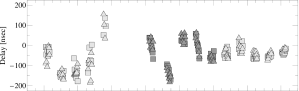
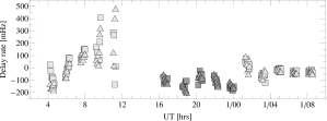
Figure 2: Residual fringe delay (top) and delay rate (bottom) solutions at 5 GHz, obtained for the SRT from the data recorded at the tracking stations in Green Bank (light gray, UT 04–12, 10 January and UT 01–08, 11 January) and Puschino (dark gray, UT 16–24, 10 January). The squares and triangles denote the solutions for the first and second IF band, respectively. The time variations of the residual delays and the delay rates likely reflect the effect of the accelerated motion of the SRT, which was not accounted for during the fringe fitting.

2.2 Post-correlation data reduction

The correlated data were reduced using AIPS for the initial calibration and Difmap (Shepherd, 1997, 2011) for imaging. The a priori amplitude calibration was applied using nominal values for the antenna gains and system temperature measurements made at each antenna during the observation. For the SRT, the sensitivity parameters measured in 2011–2013 (Kovalev et al., 2014) were used. The data were edited using the flagging information from each station log. Parallactic angle correction was applied to the ground-array antennas to account for the axis rotation of the dual-polarization antenna feeds with respect to the target source.

2.2.1 Fringe fitting

The data were fringe fit in two steps, first only for the ground array, and then also including the space baselines, with stacked solutions for the ground baselines (baseline stacking) used to improve the detectability of space baseline fringes. For the observations at 1.6 GHz, the solution interval for the ground- and space-array fringe fitting was 4 min and the cutoff $\mathrm{S/N}=3$ was set. Effelsberg was used as reference antenna for the first fringe fitting and Green Bank for the second. For the 5 GHz data, the solution interval was 1 min and 4 min for the ground and space arrays, respectively. The S/N cutoff was set to $\mathrm{S/N}=4.3$ for the ground VLBI data and $\mathrm{S/N}=3$ for the space baselines. Effelsberg was the reference antenna for all baselines. For the observations at 22 GHz, the solution intervals for the ground and space arrays were 1 min and 5 min, respectively. The S/N cutoffs and the reference antenna were the same as used for the data at 5 GHz. For the SRT, a two-way running average smoothing over a time interval of 30 minutes was applied to the solutions obtained at 5 and 22 GHz. Figure 2 shows the resulting fringe delay and delay rate solutions obtained for the SRT at 5 GHz. The solutions are consistent between the two IF bands, and the likely effect of the satellite acceleration is reflected both in the time variations of the fringe delays and in the respective delay rates. The overall behavior of the fringe solutions is in agreement with the expected accuracy of the orbital position and velocity determination (Kardashev et al., 2013; Duev et al., 2015; Lobanov et al., 2015).

2.2.2 Bandpass calibration

For the 1.6 GHz data, corrections for the individual receiver bandpasses were introduced. For this calibration, the autocorrelated data were used and phases and amplitudes were corrected. The correction was applied for the whole time interval, and Effelsberg was used as the reference antenna. For the 5 GHz and 22 GHz data, the attempted bandpass corrections did not show any improvement and were not implemented.

3 RadioAstron images of S5 0836$+$710

After the a priori amplitude calibration, fringe fitting, and bandpass calibration, the data were averaged in time over 10 s and in frequency over all channels in a given IF band and exported to Difmap for imaging and further analysis. The data were imaged using the CLEAN hybrid imaging algorithm (Högbom, 1974) and self-calibration, with amplitude adjustments limited to a single gain correction applied to each antenna over the entire duration of the respective observation. The natural weighting (increasing the sensitivity to extended emission) was applied to the visibility data for obtaining the ground array images and the uniform weighting (maximizing the image resolution) was used to produce the space VLBI images (see Briggs et al., 1999, for a detailed discussion of the data weighting in VLBI). Radial distributions of the final self-calibrated visibility amplitudes and the respective CLEAN models from the space VLBI images are plotted in Fig. 9 of Appendix A. The figures show that structure is detected up to the longest ground-space baselines and that the CLEAN models agree well with the data.

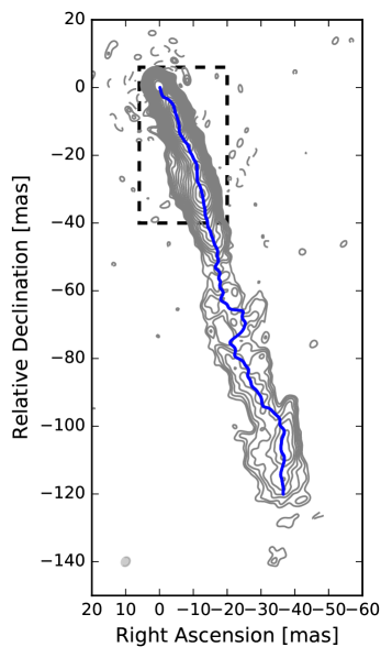
Figure 3: Ground VLBI image of S5 0836$+$710 at 1.6 GHz. Contours are drawn at ($-$1, 1, $\sqrt{2}$, 2, etc. ) times 0.32 mJy/beam. Image parameters are listed in Table 3. The dashed box marks the area covered by the respective RadioAstron image shown in Fig. 4. The curved blue line denotes the jet ridge line derived and discussed in Sect. 4.

Table 3: Parameters of the total intensity images.

$\nu$	$S_{\mathrm{tot}}$	$S_{\mathrm{peak}}$	$S_{\mathrm{neg}}$	$\sigma_{\mathrm{rms}}$	Beam
	RadioAstron images
1.6	3316	200	$-$5.4	1.30	1.200, 0.210, $-$37
5	3070	298	$-$15.0	1.50	0.146, 0.056, $-$54
22	1614	77	$-$7.9	1.03	0.035, 0.016,   77
	Ground array images
1.6	3418	1160	$-$0.8	0.15	2.880, 2.370, $-$34
5	3373	1700	$-$2.3	0.50	1.290, 0.975, $-$22
15	2429	1330	$-$1.2	0.20	0.776, 0.567,     9
22	1658	603	$-$1.6	0.30	0.388, 0.282,   $-$6
43	1171	538	$-$3.4	0.60	0.349, 0.214,   $-$3

Column designation: $\nu$ [GHz]: frequency. $S_{\mathrm{tot}}$ [mJy]: total flux density. $S_{\mathrm{peak}}$ [mJy/beam]: peak flux density. $S_{\mathrm{neg}}$ [mJy/beam]: maximum negative flux density in the image. $\sigma_{\mathrm{rms}}$ [mJy/beam]: rms noise in the image. Beam: major axis, minor axis, and position angle of major axis [mas, mas, ^∘] of the restoring beam.

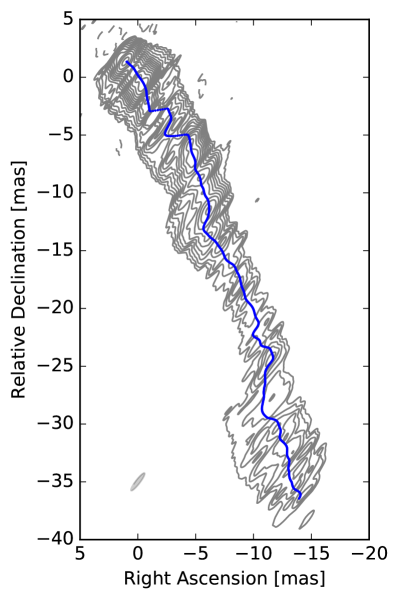
Figure 4: RadioAstron image of S5 0836$+$710 at 1.6 GHz. Contours are drawn at ($-$1, 1, $\sqrt{2}$, 2, etc. ) times 10.0 mJy/beam. Image parameters are listed in Table 3. The curved blue line denotes the ridge line we derived that is discussed in Sect. 4.

Figures 3–5 show the resulting ground-array and RadioAstron images obtained from the self-calibrated data at 1.6, 5, and 22 GHz. The respective ground array images at 15 and 43 GHz are shown in Figs. 5 and 3 of Appendix A. The parameters of all of the individual images are listed in Table 3.

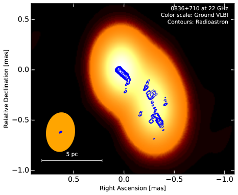
Figure 5: RadioAstron space VLBI images (contours) of S5 0836$+$710 at 5 GHz (left) and 22 GHz (right) superimposed on images obtained at respective frequencies using only the ground-array data (colors). Ground-array images are made using natural weighting and space VLBI images are made using uniform data weighting. The respective restoring beams are plotted in the lower left corner in orange (ground array) and blue (space VLBI). Basic parameters of all images are listed in Table 3.

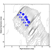
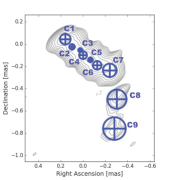
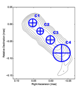
Figure 6: Gaussian components used to represent the inner jet structure observed in the RadioAstron images of S5 0836$+$710 at 1.6 GHz (left), 5 GHz (center), and 22 GHz (right). The derived component parameters are listed in Table 4.

The 1.6 GHz images from the ground-array (Fig. 3) and space VLBI (Fig. 4) data show a remarkable wealth and complexity of the structure, with the jet extending well beyond 40 mas even in the full-resolution RadioAstron image. The comparison of the space- and ground-VLBI images at 5 and 22 GHz in Fig. 5 further demonstrates the remarkable improvement in the angular resolution provided by RadioAstron. The structure traced by the space baselines is located at the brightest and most central part of the jet. The jet seen at 1.6 GHz shows wiggles that could be part of a relativistic spiral with effects from Kelvin-Helmholtz instabilities (as suggested previously in Lobanov et al., 1998; Perucho et al., 2012a, b).

The RadioAstron image at 5 GHz shows that the jet is substantially bent at small scales. Two clear bends are observed in the two brightest regions. A Kelvin-Helmholtz instability developing in the jet may explain this type of structure. The 22 GHz RadioAstron image of S5 0836$+$710 yields the highest resolution image ever obtained for this source, reaching down to $\sim 15\,\mu$as. This corresponds to a linear scale of $\sim 0.13$ pc, or $\sim 650$ gravitational radii for a black hole mass of $2\cdot 10^{9}M_{\odot}$ (Tavecchio et al., 2000). Owing to the larger errors of the visibility phase and amplitude as well as poor uv coverage on the space baselines, the full-resolution 22 GHz image can only trace the brightest regions of the jet flow, with their morphology suggesting a limb-brightened structure, which can be caused by strongly asymmetric emission within the jet, or a double-helical pattern, similar to that detected in 3C273 with VSOP observations (Lobanov & Zensus, 2001).

Table 4: Modelfit decomposition of the compact structure in S5 0836$+$710 for space-VLBI observations.

$\nu$	Comp.	$S_{\mathrm{tot}}$	$r$	$\phi$	$\theta$	$\theta_{\mathrm{min}}$	$T_{\mathrm{b}}$
[GHz]		[mJy]	[mas]	[∘]	[$\mu$as]	[$\mu$as]	[K]
1.6	C1	$70\pm 15$	$2.39\pm\;\,0.07$	$43\pm\;\,2$	$150\pm\;\,70$	107	$1.4\times 10^{12}$
	C2	$260\pm 40$	$1.66\pm\;\,0.06$	$36\pm\;\,2$	$240\pm\;\,60$	92	$2.0\times 10^{12}$
	C3	$170\pm 50$	$0.63\pm\;\,0.12$	$28\pm 11$	$310\pm 120$	124	$7.9\times 10^{11}$
	C4	$380\pm 40$	$0.11\pm\;\,0.04$	$-160\pm 20$	$230\pm\;\,40$	77	$3.3\times 10^{12}$
	C5	$640\pm 80$	$0.88\pm\;\,0.05$	$-146\pm\;\,3$	$310\pm\;\,50$	84	$3.0\times 10^{12}$
5	C1	$350\pm 10$	$0.16\pm\;\,0.02$	$74\pm\;\,4$	$50\pm\;\,20$	11	$7.3\times 10^{12}$
	C2	$90\pm 10$	$0.10\pm\;\,0.02$	$104\pm 13$	$25\pm\;\,18$	21	$7.6\times 10^{12}$
	C3	$310\pm 15$	$0.10\pm\;\,0.03$	$-180\pm\;\,8$	$35\pm\;\,18$	14	$1.3\times 10^{13}$
	C4	$160\pm 20$	$0.16\pm\;\,0.03$	$-160\pm\;\,3$	$22\pm\;\,18$	22	$1.7\times 10^{13}$
	C5	$290\pm 30$	$0.23\pm\;\,0.02$	$-150\pm\;\,2$	$39\pm\;\,17$	20	$1.0\times 10^{13}$
	C6	$320\pm 60$	$0.34\pm\;\,0.02$	$-140\pm\;\,3$	$60\pm\;\,20$	27	$4.7\times 10^{12}$
	C7	$150\pm 60$	$0.06\pm\;\,0.02$	$-150\pm 34$	$20\pm\;\,18$	38	$>5.6\times 10^{12}$
	C8	$115\pm\;\,8$	$0.58\pm\;\,0.08$	$-150\pm 15$	$86\pm\;\,17$	17	$8.2\times 10^{11}$
	C9	$6\pm\;\,1$	$0.81\pm\;\,0.08$	$-160\pm\;\,8$	$100\pm\;\,20$	25	$3.1\times 10^{10}$
22	C1	$140\pm 40$	$0.053\pm 0.007$	$85\pm\;\,8$	$12\pm\;\,\;\,7$	9	$2.4\times 10^{12}$
	C2	$110\pm 30$	$0.037\pm 0.008$	$123\pm 12$	$10\pm\;\,\;\,8$	9	$2.7\times 10^{12}$
	C3	$220\pm 50$	$0.046\pm 0.005$	$178\pm\;\,7$	$12\pm\;\,\;\,5$	8	$3.8\times 10^{12}$
	C4	$120\pm 40$	$0.090\pm 0.009$	$-159\pm\;\,6$	$25\pm\;\,\;\,9$	10	$4.7\times 10^{11}$

Notes: Gaussian model description: $S_{\mathrm{tot}}$ : total flux density. Component position in polar coordinates ($r,\,\phi$) with respect to the map center; component size, $\theta$. Minimum resolvable size, $\theta_{\mathrm{min}}$, of the respective component. Brightness temperature, $T_{\mathrm{b}}$, in the observer’s frame, derived for the parameters of the Gaussian fit.

3.1 Brightness temperature

We estimate the brightness temperature in the central regions of the jet from two-dimensional Gaussian model fitting of the visibility data, using the Levenberg-Marquardt algorithm implemented in Difmap. We compare the brightness temperatures calculated from the Gaussian modelfits with visibility-based estimates (Lobanov, 2015) obtained from the data at the longest ground-space baselines of the observations. The Gaussian modelfits of the central regions and the corresponding estimates of brightness temperature are shown in Fig. 6 and listed in Table 4.

At 1.6 GHz, a region of about 2.5 mas in extent was modeled. At the two higher frequencies, only the innermost part of the jet was modeled, limited to the structure before the first gap of emission as seen in Fig. 5. The model fitting was performed in Difmap, starting by removing the clean components in the region of interest, and replacing them with a set of fitted Gaussian components representing the respective structure.

At 1.6 GHz (left panel of Fig. 6), five components can describe the central region. For the innermost jet structure observed at 5 GHz and 22 GHz (central and right panels of Fig. 6), nine and four Gaussian components, respectively, are needed to describe the most central part. At 1.6 GHz, the entire inner jet has a brightness temperature of $\approx 10^{12}$ K, with a maximum value of $3.3\times 10^{12}$ K estimated for the component C4 located downstream from the apparent jet origin (see Table 4). At 5 GHz and 22 GHz, the respective maximum brightness temperatures are also achieved in components downstream in the jet, with $1.7\times 10^{13}$ K estimated for C4 at 5 GHz and $3.8\times 10^{12}$ K for C3 at 22 GHz. This result underlines the complex structure of the inner jet, with opacity (see Lobanov, 1998; Gómez et al., 2016), jet acceleration (Lee et al., 2016), or fine-scale substructure (e.g., resulting from recollimation shocks; see Fromm et al., 2013; Lobanov et al., 2015; Gómez et al., 2016) potentially responsible for increasing the brightness downstream from the jet base. In the reference frame of S5 0836$+$710, the respective brightness temperatures are higher by a factor of $1+z$, hence all of them exceed $10^{13}$ K and require Doppler factors, $\delta_{\mathrm{IC}}=20$–100 in order to reconcile them with the inverse Compton limit of $\approx 5\times 10^{12}$ K. Only the lower limit of the estimated $\delta_{\mathrm{IC}}$ range agrees with the kinematic Doppler factor $\delta_{\mathrm{kin}}\approx 17$ resulting from the existing measurements of the jet speed and viewing angle (Otterbein et al., 1998; Lister et al., 2013).

Table 5: Visibility-based estimates of the brightness temperature

Band	$T_{\mathrm{b,min}}$	$B$	$\langle T_{\mathrm{b,min}}\rangle$	$\langle B\rangle$
	[K]	[G$\lambda$]	[K]	[G$\lambda$]
L	$5.0\times 10^{13}$	$0.64$	$3.9\times 10^{12}$	0.66–0.73
C	$3.4\times 10^{13}$	$2.25$	$2.9\times 10^{12}$	2.34–2.60
K	$1.2\times 10^{13}$	$11.2$	$5.8\times 10^{12}$	10.4–11.5

Notes: $T_{\mathrm{b,min}}$ : minimum brightness temperature obtained from the visibility data at a given baseline length. $B$. $\langle T_{\mathrm{b,min}}\rangle$ : average value of the minimum brightness temperature over the baselines in the interval $\langle B\rangle$ corresponding to the longest 10% of the baselines in the respective data sets.

Estimating the brightness temperature directly from the visibility data (see Table 5) yields even higher values, with the minimum brightness temperature, $T_{\mathrm{b,min}}$ exceeding $10^{13}$ K at all three bands. When averaged over 10 % of the longest baselines in each data sets, the values of $T_{\mathrm{b,min}}$ approach the modelfit estimates, but still remain higher. This may be viewed as another indication that there is an ultracompact structure in the jet that is not recovered by the Gaussian modelfit. The visibility-based estimates require Doppler factors of up to $\sim 300$ to avoid the inverse Compton catastrophe. We therefore conclude that the RadioAstron observations of S5 0836$+$710 are indicative of intrinsic violation of the Compton limit on the brightness temperature.

Similar indications have also been seen in a number of other sources observed with RadioAstron (see Lobanov et al., 2015; Gómez et al., 2016; Giovannini et al., 2018), and they might imply that the innermost regions of the jet are either not in equipartition or subject to more peculiar physical conditions (Kellermann, 2002) such as a monoenergetic electron energy distribution (Kirk & Tsang, 2006). A more systematic study of the overall RadioAstron measurements of the brightness temperature should give better insights into this matter.

3.2 Asymmetries of the jet structure

The improved resolution of the RadioAstron images at 5 GHz and 22 GHz enables detailed studies of the innermost section of the flow, on scales smaller than 1 mas. The 22 GHz image presented in Fig. 5 suggests that the jet is transversally resolved, with a filamentary structure tracing only one side of the flow. This apparent asymmetric transverse structure may in part be due to the limited dynamic range (estimated to be about 75:1) of the images. It may also result from differential Doppler boosting of the flow within the jet. Following Rybicki & Lightman (1979) (see also Aloy et al., 2000; Lyutikov et al., 2005; Clausen-Brown et al., 2011), the bright side of the jet changes from top to bottom at a critical viewing angle given by $\cos(\theta_{\mathrm{r}})=\beta_{\mathrm{j}}$ for a helical magnetic field with its maximum asymmetry when the pitch angle is $45^{\circ}$. In the case of S5 0836+710, this corresponds to $\theta_{\mathrm{r}}=4^{\circ}$. Therefore, the top side of the jet should be brighter, with the estimated jet viewing angle of $3.2^{\circ}$ smaller than $\theta_{\mathrm{r}}$. This is indeed the case, as observed in Fig. 5, implying a helical field oriented counterclockwise (e.g., Aloy et al., 2000). Maximum asymmetry is obtained at $\theta^{{}^{\prime}}=\phi$, with $\theta^{{}^{\prime}}$ the viewing angle in the jet reference frame and $\phi$ the pitch angle in the fluid frame (Aloy et al., 2000). Fixing the viewing angle to $3^{\circ}$ and $\beta_{\mathrm{j}}$ to that corresponding to Lorentz factor $\gamma=12$ ($\beta_{\mathrm{j}}=0.99652$), we obtain $\phi\simeq 64^{\circ}$ for a maximum asymmetry. This pitch angle implies the presence of a helical field with a slightly dominating toroidal component. Nonetheless, the asymmetry in emission could also indicate a physical asymmetry in the jet properties, revealing the presence of distinct regions that vary across the jet channel with time. This has been revealed by a number of VLBI observations that show components that only partially fill the jet cross-section, and the jet is only observed in its full width in stacked images over many epochs (e.g., Lister et al., 2013; Pushkarev et al., 2017; Beuchert et al., 2018).

Figure 7: Relations between the jet top- and bottom-edge viewing angles $\theta_{\mathrm{t}}$ and $\theta_{\mathrm{b}}$ (left panel) and the relative azimuthal velocity $v_{\phi}/c$ (right panel) required to explain a Doppler factor ratio of 5 (solid line) and 10 (dashed line).

We can take the dynamic range of the 22 GHz image as a measure of the difference in brightness across the jet. Asymmetries in the transverse structure of the jet emission could be caused by pressure differences (Perucho et al., 2007, 2012b). However, this effect alone cannot explain this difference in brightness if the perturbation is still developing in the linear regime (Perucho et al., 2005, 2006), and the effect of the magnetic field orientation in the jet frame on the synchrotron emissivity needs to be taken into account. Nonlinear effects such as large instability amplitudes are not expected this close to the jet base unless they respond to the development of short-wavelength fast-growing modes (e.g., Perucho & Lobanov, 2007). However, in this case, we would expect a persistent and symmetric emissivity. We thus exclude the option that instability patterns generate this strong asymmetry in brightness.

We focus our discussion on the possibility that the asymmetry (of about the dynamic range of the observation) is produced by differential Doppler boosting. The observed flux density is given by

$$S_{\nu}\propto D^{2+\alpha}\,B^{\prime 1+\alpha}\,\sin(\theta^{\prime}_{\mathrm{B}}),$$ (1)

where $D$ is the Doppler factor, $B^{\prime}$ and $\theta^{\prime}_{\mathrm{B}}$ are the intensity of the magnetic field and the angle between the magnetic field and the line of sight in the fluid frame, respectively, and $\alpha$ is the spectral index ($S_{\nu}\propto\nu^{-\alpha}$). In this expression we ignore the dependence on the particle energy distribution (in particular, on the Lorentz factor limits of this distribution, $\gamma_{\mathrm{min}}$ and $\gamma_{\mathrm{max}}$, which introduce dependencies on other parameters, such as the particle number density). Recalling that the inner jet region has a flat spectral index, $\alpha\simeq 0$ (see Lobanov et al., 2006), and assuming that the total magnetic field intensity (as given by both the toroidal and poloidal components of the field) does not change much with the toroidal angle (implicitly assuming axisymmetry), we obtain the following expression for the brightness ratio between the top brighter (at least by a factor of $\approx$75) part of the jet (indicated with the superscript t) and the bottom part of the jet (superscript b) in terms of the differential Doppler factors, $D$:

$$\frac{S_{\nu,\mathrm{t}}}{S_{\nu,\mathrm{b}}}\simeq\frac{D_{\mathrm{t}}^{2}\sin(\theta^{\prime}_{\mathrm{B,t}})}{D_{\mathrm{b}}^{2}\sin(\theta^{\prime}_{\mathrm{B,b}})}\gtrsim 75\,,$$ (2)

and in the following discussion, we assume this ratio to be $\sim 100$.

Taking into account that $\sin(\theta^{\prime}_{\mathrm{B}})\,=\,D\,\sin(\theta_{\mathrm{B}})$ (the unprimed value refers to the value in the observer’s frame), we obtain

$$\frac{S_{\nu,\mathrm{t}}}{S_{\nu,\mathrm{b}}}\simeq\frac{D_{\mathrm{t}}^{3}\sin(\theta_{\mathrm{B,t}})}{D_{\mathrm{b}}^{3}\sin(\theta_{\mathrm{B,b}})}\sim 100\,.$$ (3)

The terms $D_{\mathrm{t}}$ and $D_{\mathrm{b}}$ can only be different if there is a toroidal component of the velocity and henceforth the velocity vector changes across the jet.

When we assume that the axial velocity component $v_{z}\simeq c$ is constant across the jet, the brightness asymmetry can be ascribed to the top-to-bottom change of the angle $\theta$ between the velocity vector and the line of sight, so that from Eq. 3,

$$\frac{D_{\mathrm{t}}}{D_{\mathrm{b}}}\simeq\frac{1-\cos(\theta_{\mathrm{b}})}{1-\cos(\theta_{\mathrm{t}})}\simeq 5\left(\frac{\sin(\theta_{\mathrm{B,b}})}{\sin(\theta_{\mathrm{B,t}})}\right)^{1/3},$$ (4)

which allows us to derive $\theta_{\mathrm{t}}$ in terms of $\theta_{\mathrm{b}}$ if we approximate $\left(\sin(\theta_{\mathrm{B,b}})/\sin(\theta_{\mathrm{B,t}})\right)^{1/3}\sim 1$ . The result is shown in the left panel of Fig. 7 for the Doppler factor ratios of 5 (solid line) and 10 (dashed line). In the plot, $\theta_{\mathrm{b}}$ spans from $0^{\circ}$ to 10^∘ in the observer’s frame. The required changes in the viewing angle can give estimates of the relative values of the toroidal velocity component, $v_{\phi}$, as $v_{\phi}/v_{z}\,=\,\tan(\psi)$, with $\psi$ defined as the deprojection of the half-angle formed by the velocity vectors on both sides of the jet (here we assumed a mean viewing angle of $3^{\circ}$ to deproject the half-angle between the velocity vectors). This ratio is plotted in the right panel of Fig. 7 for the same Doppler factor ratios. The plots show that low toroidal velocities can result in sufficiently large changes in the Doppler factor of different regions in the flow.

When we assume in contrast that $D_{\mathrm{t}}\simeq D_{\mathrm{b}}$, then the brightness asymmetry has to be given by

$$\frac{S_{\nu,\mathrm{t}}}{S_{\nu,\mathrm{b}}}\simeq\frac{\sin(\theta^{\prime}_{\mathrm{B,t}})}{\sin(\theta^{\prime}_{\mathrm{B,b}})}\simeq 100\,.$$ (5)

Taking into account that this ratio $\sin(\theta^{\prime}_{\mathrm{B,t}})/\sin(\theta^{\prime}_{\mathrm{B,b}})\,\simeq\,\sin(\theta_{\mathrm{B,t}})/\sin(\theta_{\mathrm{B,b}})$ ($D^{\mathrm{t}}\simeq D^{\mathrm{b}}$) and that $0\leq\sin(\theta_{\mathrm{B}})\leq 1$, the fraction can only give a value $\simeq 100$ if one or both values of $\theta_{\mathrm{B}}$ are very close to $0^{\circ}$, where the sine can take values that differ by several orders of magnitude. We find this coincidence that both angles are aligned to such an accuracy less probable than the presence of low toroidal velocities. Furthermore, a toroidal component of the velocity has been shown to naturally arise in RMHD simulations of expanding jets due to the Lorentz force (Martí et al., 2016). Finally, the required azimuthal velocities are compatible with the axial velocity (Lorentz factor) reported for this jet (Perucho et al., 2012a) in terms of causality. We can conclude that a low toroidal velocity has to be present in the jet flow to explain the brightness asymmetry. Recent numerical GRMHD simularions of jet formation (McKinney & Blandford, 2009; McKinney et al., 2012) indicated that the rotational speed reaches up to the Keplerian speed, $v_{\mathrm{c}}(r_{\mathrm{j}})$, at a given jet radius, $r_{\mathrm{j}}$. For the reported black hole mass of $2\times 10^{9}\,\mathrm{M}_{\odot}$ (Tavecchio et al., 2000) and a jet radius $r_{\mathrm{j}}\approx 0.05$ mas ($\approx 0.4$ pc) estimated from the RadioAstron images, the respective $v_{\mathrm{c}}\approx 0.015$ c is substantially higher than the $v_{\phi}$ estimates made above. This may result from a slowdown due to thermal mixing or shear, but likely uncertainties in all of the measured quantities involved in these calculations preclude us form making any firm conclusion on the matter. We plan to run RMHD simulations to further investigate the potential physical mechanisms that define the estimated rotation in this jet.

4 Jet structure: Ridge line oscillations

4.1 Ridge line calculation

Because of the limited dynamic range of the space VLBI images at 5 GHz and 22 GHz (in which the jet is transversally resolved), we base our quantitative analysis of the jet flow largely on the jet ridge line derived from the 1.6 GHz images of S5 0836+710. At the scales sampled by these images, plasma instability is expected to play an important role, inducing regular patterns into the flow. We study these patterns by estimating the ridge line of the jet. We define the jet ridge as the line that connects the peaks of one-dimensional Gaussian profiles fitted to the profiles (slices) of the jet brightness drawn orthogonally to the jet direction (see Lobanov et al., 1998; Perucho et al., 2012a, for similar previous studies), with the step between individual profiles set to be smaller than the beam size (a measure taken in order to ensure continuity of the brightness profiles recovered from adjacent slices). Similarly to the earlier studies of S5 0836+710, a position angle of $-$162^∘ was adopted for the jet direction. To obtain the ridge line, a code was developed using Python and the iMinuit package. The fitting algorithm implements continuity conditions for the parameters fitted to adjacent slices, thus ensuring a robust and self-consistent description of the evolution of the ridge line and flow width along the jet. The first slice is taken across the jet so as to cross the peak of brightness in the image at a given frequency. We calculated the uncertainties of the fitted parameters from the S/N in the image using the method described in Schinzel et al. (2012).

We present the ridge lines obtained from the ground- and space-VLBI images of S5 0836+710 at 1.6 GHz in Figs. 3–4. The ridge lines obtained from the images at other frequencies are presented in Appendix A.

The complex ridge line structure suggests the presence of several periodic patterns in the flow. In the following, we assume that these oscillatory modes represent individual modes of Kelvin-Helmholtz (KH) instability developing in the flow (see Lobanov & Zensus, 2001; Perucho & Lobanov, 2007; Perucho et al., 2012a).

4.2 Modeling the KH instability modes

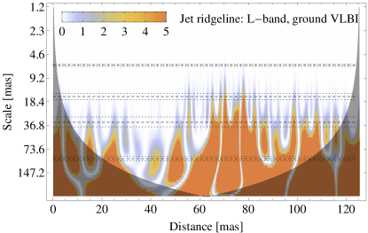
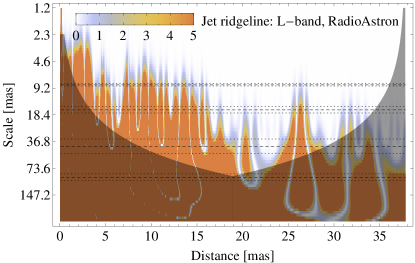
Figure 8: Wavelet scalograms for the ridge lines of S5 0836+710 at 1.6 GHz, obtained from the ground- (left) and space-VLBI (right) images. Color presents the wavelet amplitude scaled with the mean error, $\sigma_{\mathrm{pos}}$, of the ridge line position measurements. The color scale is saturated at $5\,\sigma_{\mathrm{pos}}$ level for better viewing. Undersampled regions of the parameter space are shaded. For both ridge lines, the scalogram is dominated by an oscillation with a long wavelength of $\sim 90$–$100$ mas, although it cannot be well sampled with the ridge line from the space-VLBI image. Presence of one or more oscillatory patterns with wavelengths of $\sim 25$–$45$ mas can also be suggested from both scalograms. A mode with the wavelength of $\sim 10$–$15$ mas can be inferred from the space-VLBI ridge line. For the purpose of comparison, each scalogram also shows the wavelengths (dashed lines) and respective uncertainties (dotted lines) of the oscillatory modes fitted to represent the ridge lines as described in Section 4.2. For each of these wavelengths, the respective scalogram contains at least one region of statistically significant wavelet amplitudes, thus reaffirming the physical relevance of the fitted oscillatory modes.

We initially identifed the potential modes using a wavelet scalogram calculated from the ridge line offsets measured in the ground- and space-VLBI images at 1.6 GHz (Fig. 8), with the Marr function as the kernel for the wavelet transform. The scalograms presented in Fig. 8 indicate oscillatory modes at wavelengths of $\sim$ 90 mas, $\sim$ 35 mas, $\sim$ 15 mas, and $\sim$ 10 mas. The wavelet scalograms also show that the oscillatory patterns may have a slightly increasing wavelength with distance, a typical behavior expected for a KH mode propagating in an expanding flow (Hardee, 2000). These inferences are used as initial guesses for further modeling of the ridge lines.

We used the ridge line measured in the 1.6 GHz ground- and space-array images as the basis for our modeling. We first describe the observed offset, $\Delta\,r(z)$, of the ridge line with a simplified model by fitting it with several different oscillatory terms with constant amplitudes and wavelengths:

$$\Delta\,r(z)=\sum_{i=1}^{N_{\mathrm{mod}}}a_{i}\sin(2\,\pi/\lambda_{i}+\psi_{i})\,,$$ (6)

where $a_{i}$ is the amplitude, $\psi_{i}$ the phase and $\lambda_{i}$ the wavelength corresponding to the $i$-th mode. Four modes were needed to minimize the $\chi^{2}$ in both ridge lines. The fitting was performed in two ways:

1. Fitting the first mode and subtracting it from the original ridge line. Then, a second mode was fit and again subtracted. The process was iterated until the addition of a new mode did not provide any improvement to the fit.

2. Fitting all modes at the same time. This method depends more strongly on the initial guess parameters. The first three modes were fit with the wavelengths observed in the scalogram as an initial guess.

For both methods, the best fit was chosen to be that which reduced the $\chi^{2}$. The two methods yield similar results. The wavelengths of the modes are listed in Table 6 for the ground-image ridge line and in Table 7 for the space-VLBI image ridge line. Figure 9 shows the resulting fit for the two ridge lines. The resulting wavelengths obtained from two independent fits are similar in both cases. This corroborates the robustness of our identification of the oscillatory modes and the little role played by jet expansion on the wavelength, taking into account the small jet opening angle ($<1^{\circ}$ Perucho et al., 2012a).

Table 6: Oscillatory mode representation of the ridge line in the ground-array L-band image

Mode	$\lambda$ [mas]	$a$ [mas]	$\psi$ [∘]
1	$102.0\pm 6.0$	$2.90\pm 0.20$	$15\pm\;\;8$
2	$35.0\pm 5.0$	$0.21\pm 0.03$	$195\pm 50$
3	$16.5\pm 1.5$	$0.55\pm 0.16$	$-105\pm 30$
4	$6.6\pm 0.2$	$0.30\pm 0.05$	$146\pm 11$

Table 7: Oscillatory mode representation of the ridge line in the RadioAstron L-band image

Mode	$\lambda$ [mas]	$a$ [mas]	$\psi$ [∘]
1	$97.0\pm 4.0$	$3.70\pm 0.20$	$0\pm 10$
2	$44.0\pm 8.0$	$0.42\pm 0.04$	$82\pm 14$
3	$16.9\pm 1.4$	$0.50\pm 0.12$	$-106\pm\;\;7$
4	$8.8\pm 0.1$	$0.23\pm 0.07$	$54\pm\;\;6$

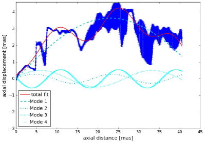
Figure 9: Fits by oscillatory modes to the jet ridge lines in the ground- (left) and space- (right) VLBI images of S5 0836+710 at 1.6 GHz. In each plot, the red line is the total multi-mode fit and the blue lines represent contributions from the individual oscillatory modes as described in the legend.

When we compare these results with earlier works, it is interesting to note that the wavelengths identified in the ridge line at 1.6 GHz agree well with those that were obtained previously from the VSOP image of the source (Lobanov et al., 1998), where oscillations with wavelengths of $\simeq 100$, $\sim 8$, and $\sim 5$ mas were identified. The longest of these wavelengths is reasonably close to the $\lambda=97$ or $\lambda=102$ mas of the mode 1 in our RadioAstron data, and the two shorter wavelengths are close to $\lambda=6.6$ mas from the ground-array image and $\lambda=8.8$ mas of the mode 4 from the space-VLBI image. It should be noted that identification of short wavelengths in a ridge line measured in different VLBI images can be affected by the differences in the image noise and the uv coverage of the observations. It is therefore more difficult to give a robust representation of short-wavelength oscillations in a ridge line. We note that a $\simeq 80$ mas mode was also detected in VLBA images of S5 0836+710 by Perucho et al. (2012a), who suggested the presence of oscillations with shorter and possibly variable wavelengths, and reported oscillations with a wavelength between $\simeq 10$ mas and $\simeq 20$ mas at $r\leq 40$ mas distance from the jet origin and growing to $\simeq 40$ mas at $r\geq 40$ mas. Finally, Perucho et al. (2012a) also reported the detection of short-wavelength oscillations, with wavelengths $\simeq 5$ mas at $r<15$ mas increasing to $\simeq 7$–$8$ mas at $r>20$ mas. These can be related to mode 4 in Tables 6 and 7 (wavelengths of 6.6 and 8.8 mas). It is also relevant to stress that in our fits we did not include growth lengths for the modes, which can also introduce small differences with the data at the largest scales. Based on all these arguments, we conclude that our results are consistent with previous studies of the instability patterns detected in the jet of S5 0836+710.

Regarding the possible identification of the instability modes, because the first, longest-wavelength mode displaces the ridge line, it should correspond to a helical mode. It could be tentatively identified as an helical surface mode, $H_{\mathrm{s}}$.

A tentative identification of the other modes can be obtained using the characteristic wavelength, $\lambda^{*}=\lambda_{i}(n_{i}+2m_{i}+\frac{1}{2})$, where $\lambda^{*}$ is the characteristic wavelength, $\lambda_{i}$ the observed wavelength and $n_{i}$ and $m_{i}$ the two transverse wavenumbers of the mode. The characteristic wavelength should have a similar value for the different modes (Lobanov & Zensus, 2001), assuming that all the observed wavelengths correspond to modes that are excited at their maximum growth rates. The second-longest wavelength should then be the first helical body mode, $H_{\mathrm{b1}}$, whereas the third longest wavelength should be either the second, $H_{\mathrm{b2}}$, or the third helical body mode, $H_{\mathrm{b3}}$. We exclude the fourth mode because such small wavelengths are difficult to determine and the results for ground and space arrays do not reconcile, even when the errors are accounted for. For the case in which the third mode is identified as the second-order helical body mode, the characteristic wavelength is $119\pm 12$ mas, and when the third mode is identified as the third-order body mode, the characteristic wavelength is $130\pm 12$ mas.

Following the approach of Hardee (2000) and references therein, the basic physical parameters of the jet can be obtained from the identification of the different modes, using the linear analysis of the Kelvin-Helmholtz instability. With this approach, it is possible to obtain the Mach number of the jet and the ratio of the jet to the ambient density knowing the characteristic wavelength, the jet radius, jet viewing angle, the jet apparent speed, and the apparent pattern speed. The jet radius can be easily calculated. It corresponds to the point where the peak flux density of the jet is reduced to $1\%$ along the jet direction (Wehrle et al., 1992).

In practice, to choose the slice where we measure the jet width, we considered the slice with a peak flux density $1\%$ of the flux density of the first slice, corresponding to the brightest point of the jet. For this slice, we took the full width at half-maximum (FWHM) of the corresponding Gaussian profile as a measure of the jet width. Then we deconvolved it, using the following relation: $R_{\mathrm{j}}{\mathrm{[mas]}}=0.5\sqrt{\theta_{\mathrm{FWHM}}^{2}-b^{2}}$, where $\theta_{\mathrm{FWHM}}$ is the FWHM of the corresponding slice and $b$ is the beam size. This yields a jet radius of $2$ mas or $16$ pc. We note that in earlier works (Perucho & Lobanov, 2007, 2011) a substantially higher value of 17 mas was estimated for the jet radius. This value corresponds to the apparent jet radius measured directly from the image, while we deconvolved this measurement with the FWHM of the resolving beam. The large radius considered in earlier works led to the identification of the longest observed wavelength with the first body mode (because the observed structures are relatively shortened when they are measured with respect to the jet radius).

For the jet viewing angle and for the speed we used the values given in Otterbein et al. (1998), that is: $\theta_{\mathrm{j}}=3^{\circ}$ , and a Lorentz factor $\gamma_{\mathrm{j}}=12$, which corresponds to an apparent speed of $\beta_{\mathrm{app}}=10.7$. The apparent pattern speed was measured by comparing ridge lines for different epochs at $15$ GHz in the images of the MOJAVE monitoring program. This calculation was made using only the highest S/N region at 1–4 mas distances from the jet origin. The measured speed was $w_{\mathrm{app}}=0.35\pm 0.25c$. With these quantities, the Mach number $M_{\mathrm{j}}$ and the ratio of the jet to the ambient density $\eta$ can be calculated as (e.g., Hardee, 2000)

$$M_{\mathrm{j}}=\frac{\lambda^{*}(1-\beta_{w}\cos{\theta_{\mathrm{j}}})}{8R_{\mathrm{j}}\gamma_{\mathrm{j}}(1-\beta_{w}/\beta_{\mathrm{j}})\sin{\theta_{\mathrm{j}}}}\,,$$ (7)

$$\eta=\frac{M_{\mathrm{j}}^{2}}{M_{\mathrm{x}}^{2}},$$ (8)

where the external jet Mach number, $M_{\mathrm{x}}$, and the intrinsic jet pattern speeds are calculated with

$$M_{\mathrm{x}}=\frac{\lambda^{*}\beta_{\mathrm{j}}(1-\beta_{w}\cos{\theta_{\mathrm{j}}})}{8R_{\mathrm{j}}\beta_{w}\sin{\theta_{\mathrm{j}}}}\,,$$ (9)

$$\beta_{w}=\frac{w_{\mathrm{app}}}{\sin{\theta_{\mathrm{j}}}+w_{\mathrm{app}}\cos{\theta_{\mathrm{j}}}}\,,$$ (10)

and

$$\beta_{\mathrm{j}}=\frac{\beta_{\mathrm{app}}}{\sin{\theta_{\mathrm{j}}}+\beta_{\mathrm{app}}\cos{\theta_{\mathrm{j}}}}.$$ (11)

This yields a Mach number of $M_{\mathrm{j}}=12\pm 3$, in contrast to the results given in Lobanov et al. (1998), who reported a Mach number of 6 and a density ratio of $\eta=0.33\pm 0.08$. The ratio of the jet to the ambient density we obtained here is close to unity, which may indicate that the jet is surrounded by a very diluted cocoon. This restriction could be alleviated if the pattern speed we used represents an upper limit because the different modes travel at different speeds; the shorter wavelength modes travel faster. Taking into account that the pattern speed was calculated in a rather small region, it therefore probably corresponds to a mode with a small wavelength, which is difficult to measure. The effect of the speed on the ratio of the jet to the ambient density is also relevant. If we look at different values within the range allowed by the error, for example assuming a pattern speed of $w_{\mathrm{app}}=0.10c$, the ratio of the jet to the ambient density changes by an order of magnitude, to $\eta\sim 0.02$. Nevertheless, the jet Mach number remains unchanged. Another important remark is that the approximation used before is only valid for cases where $M_{\mathrm{j}}\gg 1$, which is verified by our result, and in the scenario where a contact discontinuity (or a narrow shear-layer) separates the jet and the ambient medium. The possibility of a shear layer playing a role in the jet in S5 0836+710 has been suggested in earlier works (Perucho & Lobanov, 2007, 2011) after solving the linear stability problem for sheared jets, using a set of jet parameters given by Lobanov et al. (1998). Arising naturally in spine-sheath scenarios, such a shear layer will also affect the growth rates and wavelengths of the KH instability modes (see Mizuno et al., 2007; Hardee, 2007).

5 Summary

Multiband VLBI observations of S5 0836+710 with RadioAstron provided images of the jet with an unprecedentedly high angular resolution, reaching down to 15 microarcseconds at 22 GHz, which corresponds to a linear scale of 0.13 pc. The radio source S5 0836+710 was observed with a ground- and space-VLBI array at the frequencies of 1.6 GHz on 24 October 2013, and 5 and 22 GHz on 10 January 2014. The source was observed with tracks of 16.5 hours at 1.6 GHz and over a 30-hour period (with a 4-hour gap) at 5 and 22 GHz.

Non-standard procedures were needed to detect interferometric fringes with the space antenna; the resulting residual delay solutions for the 5 GHz RadioAstron image are shown in Fig. 2. They show a weak time-dependence due to the acceleration of the space antenna. The source was detected on baselines as long as 10 Earth diameters at 1.6 GHz, and 12 Earth diameters at 5 GHz and 22 GHz.

Hybrid imaging was performed for the ground- and space-array data. The latter yield resolutions of 3 to 10 times the ground resolution, reaching scales of $\sim 15\,\mu$as ($\sim 0.12$ pc) at 22 GHz. The full-resolution RadioAstron images show a much richer structural detail than the ground-array images at the same frequencies. At 5 GHz and 22 GHz, the jet is transversely resolved in the RadioAstron images, revealing a bent and asymmetric pattern embedded into the flow.

The observed brightness temperature of the jet is estimated for the three frequencies and is listed in Table 4. These estimates indicate that the highest brightness temperatures for each frequency are $3.3\times 10^{12}$ K, $1.7\times 10^{13}$ K, and $3.8\times 10^{12}$ K for 1.6 GHz, 5 GHz, and 22 GHz, respectively. These estimates agree well with the minimum brightness temperature estimated from the visibility data, using the longest $10$ $\%$ baselines. All of the estimates imply $T_{\mathrm{b}}\geq 10^{13}$ K in the reference frame of the source and would require Doppler factors of up to $\sim 300$ in order to reconcile them with the inverse Compton limit.

The internal structure of the jet was studied by analyzing the ridge line of the jet. For the lowest frequency of 1.6 GHz, the location of the ridge line observed in the ground-array and space-VLBI images were obtained by fitting transverse brightness profiles with a single-Gaussian component and recording the position of its peak with respect to the overall jet axis oriented at a position angle of $-$162^∘. The ridge lines were represented with a simple model as the sum of multiple oscillatory terms. The parameters of these oscillatory modes are modeled and explained in the framework of a Kelvin-Helmholtz instability that develops in the flow. The wavelengths of the oscillations are found to be similar to those reported in previous studies of the source. These oscillations can be interpreted as resulting from the helical modes of the instability developing in the jet. Based on this interpretation, an estimate of the jet Mach number and the ratio of the jet to the ambient density is obtained of $\sim 12$ and $\sim 0.33,$ respectively. This estimate can be further verified and refined using a more detailed numerical analysis of the jet stability.

Appendix A Auxiliary plots: uv coverage, visibility amplitudes, hybrid images, and jet ridge lines.

This appendix presents auxiliary information and images obtained from the RadioAstron observations. Ridge lines determined from RadioAstron images at 5 GHz and 22 GHz are shown in Figs. 10–2. The ground -array images and respective ridge lines at 43, 22, 15, and 5 GHz are presented in Figs. 3–6. The uv coverage of the accompanying ground-array observations at 15 and 43 GHz are shown in Figs. 7–8. Radial distributions of the visibility amplitudes measured in the RadioAstron observations at 1.6, 5, and 22 GHz are given in Fig. 9.

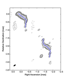
Figure 10: Ridge line in the RadioAstron image of the jet in S5 0836$+$710 at 5 GHz shown in Fig. 5. The contour levels are drawn at ($-$1, 1, $\sqrt{2}$, 2, etc. ) times 7.0 mJy/beam. Image parameters are given in Table 3. A discussion of the jet ridge lines is presented in Sect. 4.

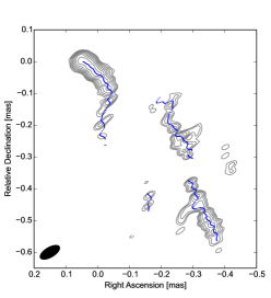
Figure 2: Ridge line in the RadioAstron image of the jet in S5 0836$+$710 at 22 GHz shown in Fig. 5. The contour levels are drawn at ($-$1, 1, $\sqrt{2}$, 2, etc. ) times 5.0 mJy/beam. Image parameters are given in Table 3. A discussion of the jet ridge lines is presented in Sect. 4.

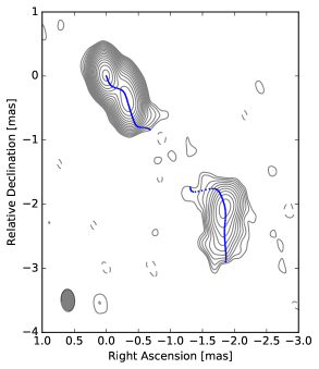
Figure 3: Image of the jet in S5 0836$+$710 made from the ground-VLBI data at 43 GHz. The contour levels are drawn at ($-$1, 1, $\sqrt{2}$, 2, etc. ) times 1.8 mJy/beam. The curved blue line denotes the ridge line of the jet we derived that is discussed in Sect. 4.

Figure 5: Image of the jet in S5 0836$+$710 made from the ground-VLBI data at 15 GHz. The contour levels are drawn at ($-$1, 1, $\sqrt{2}$, 2, etc. ) times 0.75 mJy/beam. The curved blue line denotes the ridge line of the jet we derived that is discussed in Sect. 4.

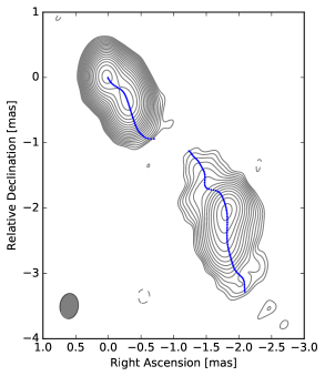
Figure 4: Image of the jet in S5 0836$+$710 made from the ground-VLBI data at 22 GHz. The contour levels are drawn at ($-$1, 1, $\sqrt{2}$, 2, etc. ) times 1.0 mJy/beam. The curved blue line denotes the ridge line of the jet we derived that is discussed in Sect. 4.

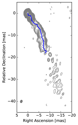
Figure 6: Image of the jet in S5 0836$+$710 made from the ground-VLBI data at 5 GHz. The contour levels are drawn at ($-$1, 1, $\sqrt{2}$, 2, etc. ) times 1.5 mJy/beam. The curved blue line denotes the ridge line of the jet we derived that is discussed in Sect. 4.

Figure 7: Coverage of the Fourier domain (uv coverage) of the ground-array observations of S5 0836$+$710 at 15 GHz plotted in units of M$\lambda$.

Figure 8: Coverage of the Fourier domain (uv coverage) of the ground-array observations of S5 0836$+$710 at 43 GHz plotted in units of M$\lambda$.

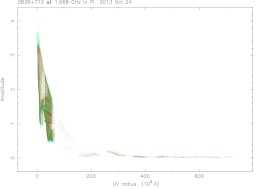
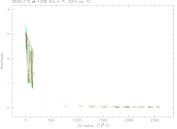
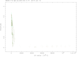
Figure 9: Radial distributions of visibility amplitudes (orange) from the RadioAstron observations of S5 0836$+$710 at 1.6 GHz (top), 5 GHz (middle), and 22 GHz (bottom) as a function of uv distance, overplotted with the respective CLEAN models (red) of the source structure.

References

- Aloy et al. (2000) Aloy, M.-A., Gómez, J.-L., Ibáñez, J.-M., Martí, J.-M., & Müller, E. 2000, ApJ, 528, L85
- Andreyanov et al. (2014) Andreyanov, V. V., Kardashev, N. S., & Khartov, V. V. 2014, Cosmic Research, 52, 319
- Arsentev et al. (1982) Arsentev, V. M., Berzhatyi, V. I., Blagov, V. D., et al. 1982, Akademiia Nauk SSSR Doklady, 264, 588
- Beuchert et al. (2018) Beuchert, T., Kadler, M., Perucho, M., et al. 2018, A&A, 610, A32
- Briggs et al. (1999) Briggs, D. S., Schwab, F. R., & Sramek, R. A. 1999, in Astronomical Society of the Pacific Conference Series, Vol. 180, Synthesis Imaging in Radio Astronomy II, ed. G. B. Taylor, C. L. Carilli, & R. A. Perley, 127
- Bruni et al. (2016) Bruni, G., Anderson, J., Alef, W., et al. 2016, Galaxies, 4, 55
- Bruni et al. (2015) Bruni, G., Anderson, J. M., Alef, W., Lobanov, A. P., & Zensus, J. A. 2015, in Proceedings of Science, Vol. EVN 2014, Proceedings of the 12th European VLBI Network Symposium, 119
- Clausen-Brown et al. (2011) Clausen-Brown, E., Lyutikov, M., & Kharb, P. 2011, MNRAS, 415, 2081
- Deller et al. (2011) Deller, A. T., Brisken, W. F., Phillips, C. J., et al. 2011, PASP, 123, 275
- Deller et al. (2007) Deller, A. T., Tingay, S. J., Bailes, M., & West, C. 2007, PASP, 119, 318
- Duev et al. (2015) Duev, D. A., Zakhvatkin, M. V., Stepanyants, V. A., et al. 2015, A&A, 573, A99
- Ford et al. (2014) Ford, H. A., Anderson, R., Belousov, K., et al. 2014, in Proceedings of the SPIE, Vol. 9145, id. 91450
- Fromm et al. (2013) Fromm, C. M., Ros, E., Perucho, M., et al. 2013, A&A, 557, A105
- Giovannini et al. (2018) Giovannini, G., Savolainen, T., Orienti, M., et al. 2018, Nature Astronomy, 2, 472
- Gómez et al. (2016) Gómez, J. L., Lobanov, A. P., Bruni, G., et al. 2016, ApJ, 817, 96
- Hardee (2000) Hardee, P. E. 2000, ApJ, 533, 176
- Hardee (2007) Hardee, P. E. 2007, ApJ, 664, 26
- Hardee & Stone (1997) Hardee, P. E. & Stone, J. M. 1997, ApJ, 483, 121
- Hirabayashi et al. (2000) Hirabayashi, H., Hirosawa, H., Kobayashi, H., et al. 2000, PASJ, 52, 955
- Högbom (1974) Högbom, J. A. 1974, A&AS, 15, 417
- Hummel et al. (1992) Hummel, C. A., Muxlow, T. W. B., Krichbaum, T. P., et al. 1992, A&A, 266, 93
- Kardashev et al. (2013) Kardashev, N. S., Khartov, V. V., Abramov, V. V., et al. 2013, Astronomy Reports, 57, 153
- Kellermann (2002) Kellermann, K. I. 2002, PASA, 19, 77
- Kettenis (2010) Kettenis, M. 2010, in 10th European VLBI Network Symposium and EVN Users Meeting: VLBI and the New Generation of Radio Arrays, 86
- Khartov et al. (2014) Khartov, V. V., Shirshakov, A. E., Artyukhov, M. I., et al. 2014, Cosmic Research, 52, 326
- Kirk & Tsang (2006) Kirk, J. G. & Tsang, O. 2006, A&A, 447, L13
- Komissarov et al. (2007) Komissarov, S. S., Barkov, M. V., Vlahakis, N., & Königl, A. 2007, MNRAS, 380, 51
- Königl (1981) Königl, A. 1981, ApJ, 243, 700
- Kovalev et al. (2014) Kovalev, Y. A., Vasil’kov, V. I., Popov, M. V., et al. 2014, Cosmic Research, 52, 393
- Krichbaum et al. (1990) Krichbaum, T. P., Hummel, C. A., Quirrenbach, A., et al. 1990, A&A, 230, 271
- Lee et al. (2016) Lee, S.-S., Lobanov, A. P., Krichbaum, T. P., & Zensus, J. A. 2016, ApJ, 826, 135
- Levy et al. (1986) Levy, G. S., Linfield, R. P., Ulvestad, J. S., et al. 1986, Science, 234, 187
- Likhachev et al. (2017) Likhachev, S. F., Kostenko, V. I., Girin, I. A., et al. 2017, Journal of Astronomical Instrumentation, 6, 1750004
- Lister et al. (2013) Lister, M. L., Aller, M. F., Aller, H. D., et al. 2013, AJ, 146, 120
- Lobanov (1998) Lobanov, A. P. 1998, A&A, 330, 79
- Lobanov (2015) Lobanov, A. P. 2015, A&A, 574, A84
- Lobanov et al. (2015) Lobanov, A. P., Gómez, J. L., Bruni, G., et al. 2015, A&A, 583, A100
- Lobanov et al. (1998) Lobanov, A. P., Krichbaum, T. P., Witzel, A., et al. 1998, A&A, 340, L60
- Lobanov et al. (2006) Lobanov, A. P., Krichbaum, T. P., Witzel, A., & Zensus, J. A. 2006, PASJ, 58, 253
- Lobanov & Zensus (2001) Lobanov, A. P. & Zensus, J. A. 2001, Science, 294, 128
- Lyubarsky (2010) Lyubarsky, Y. E. 2010, MNRAS, 402, 353
- Lyutikov et al. (2005) Lyutikov, M., Pariev, V. I., & Gabuzda, D. C. 2005, MNRAS, 360, 869
- Martí et al. (2016) Martí, J. M., Perucho, M., & Gómez, J. L. 2016, ApJ, 831, 163
- McKinney & Blandford (2009) McKinney, J. C. & Blandford, R. D. 2009, MNRAS, 394, L126
- McKinney et al. (2012) McKinney, J. C., Tchekhovskoy, A., & Bland ford, R. D. 2012, MNRAS, 423, 3083
- Mertens et al. (2016) Mertens, F., Lobanov, A. P., Walker, R. C., & Hardee, P. E. 2016, A&A, 595, A54
- Mizuno et al. (2016) Mizuno, Y., Gómez, J., Nishikawa, K.-I., et al. 2016, Galaxies, 4, 40
- Mizuno et al. (2007) Mizuno, Y., Hardee, P., & Nishikawa, K.-I. 2007, ApJ, 662, 835
- Mizuno et al. (2014) Mizuno, Y., Hardee, P. E., & Nishikawa, K.-I. 2014, ApJ, 784, 167
- Mizuno et al. (2012) Mizuno, Y., Lyubarsky, Y., Nishikawa, K.-I., & Hardee, P. E. 2012, ApJ, 757, 16
- Nakamura & Meier (2004) Nakamura, M. & Meier, D. L. 2004, ApJ, 617, 123
- Osmer et al. (1994) Osmer, P. S., Porter, A. C., & Green, R. F. 1994, ApJ, 436, 678
- Otterbein et al. (1998) Otterbein, K., Krichbaum, T. P., Kraus, A., et al. 1998, in Astronomical Society of the Pacific Conference Series, Vol. 144, IAU Colloq. 164: Radio Emission from Galactic and Extragalactic Compact Sources, ed. J. A. Zensus, G. B. Taylor, & J. M. Wrobel, 73
- Perucho (2019) Perucho, M. 2019, Galaxies, 7, 70
- Perucho et al. (2007) Perucho, M., Hanasz, M., Martí, J.-M., & Miralles, J.-A. 2007, Phys. Rev. E, 75, 056312
- Perucho et al. (2012a) Perucho, M., Kovalev, Y. Y., Lobanov, A. P., Hardee, P. E., & Agudo, I. 2012a, ApJ, 749, 55
- Perucho & Lobanov (2007) Perucho, M. & Lobanov, A. P. 2007, A&A, 469, L23
- Perucho & Lobanov (2011) Perucho, M. & Lobanov, A. P. 2011, A&A, 533, C2
- Perucho et al. (2005) Perucho, M., Lobanov, A. P., & Martí, J. M. 2005, Mem. Soc. Astron. Italiana, 76, 110
- Perucho et al. (2006) Perucho, M., Lobanov, A. P., Martí, J.-M., & Hardee, P. E. 2006, A&A, 456, 493
- Perucho et al. (2012b) Perucho, M., Martí-Vidal, I., Lobanov, A. P., & Hardee, P. E. 2012b, A&A, 545, A65
- Planck Collaboration et al. (2016) Planck Collaboration, Ade, P. A. R., Aghanim, N., et al. 2016, A&A, 594, A13
- Pushkarev et al. (2017) Pushkarev, A. B., Kovalev, Y. Y., Lister, M. L., & Savolainen, T. 2017, MNRAS, 468, 4992
- Rybicki & Lightman (1979) Rybicki, G. B. & Lightman, A. P. 1979, Radiative processes in astrophysics (New York, Wiley-Interscience)
- Schinzel et al. (2012) Schinzel, F. K., Lobanov, A. P., Taylor, G. B., et al. 2012, A&A, 537, A70
- Shepherd (2011) Shepherd, M. 2011, Difmap: Synthesis Imaging of Visibility Data, Astrophysics Source Code Library
- Shepherd (1997) Shepherd, M. C. 1997, in Astronomical Society of the Pacific Conference Series, Vol. 125, Astronomical Data Analysis Software and Systems VI, ed. G. Hunt & H. Payne, 77
- Tavecchio et al. (2000) Tavecchio, F., Maraschi, L., Ghisellini, G., et al. 2000, ApJ, 543, 535
- Torrealba et al. (2012) Torrealba, J., Chavushyan, V., Cruz-González, I., et al. 2012, Rev. Mexicana Astron. Astrofis., 48, 9
- Vega-García et al. (1998) Vega-García, L., Perucho, M., & Lobanov, A. P. 1998, A&A, 330, 79
- Vlahakis & Königl (2004) Vlahakis, N. & Königl, A. 2004, ApJ, 605, 656
- Wehrle et al. (1992) Wehrle, A. E., Cohen, M. H., Unwin, S. C., et al. 1992, ApJ, 391, 589
- Zakhvatkin et al. (2014) Zakhvatkin, M. V., Ponomarev, Y. N., Stepan’yants, V. A., Tuchin, A. G., & Zaslavskiy, G. S. 2014, Cosmic Research, 52, 342