Slice collective dynamics, projected emittance deterioration and Free Electron Laser performances detrimental effects

Abstract

The dynamical effects inducing geometrical and phase space misalignment of bunch slice in X-ray operating Free Electron Lasers can be traced back to a plethora of phenomena, both in the linac accelerating section or inside the beam transport optic magnet. They are responsible for a spoiling of the beam projected qualities and induce, if not properly corrected, an increase of the saturation length and a decreasing of the output power. We discuss the inclusion of these effects in models employing scaling formulae.

I Introduction

In forty years of research it has emerged that the physics of Free Electron Laser (FEL) and the relevant design can be afforded by the use of numerical codes capable of including as much as physics is possible (giannessi2003, 1, ). On the other side a particular useful role has been played by a set of semi-analytical relations, called, perhaps improperly, scaling formulae (MXie, ; dattoli-letardi1984, ; dattoli-caloi1989, ; BookletFEL, ; SaldinModel, ). This last tool has been developed, “optimized” along the course of the years and benchmarked through a wise combination of theoretical concepts, numerical methods and comparison with the experiment.

The use of scaling formulae cannot replace that of dedicated codes, but it can be helpful to fix the design working points and specify how the various pieces of the game should be embedded. The strength of this procedure stems from the fact that the method gathers together the various parameters entering the definition of the FEL dynamics by picking out those representative dimensionless global quantities capable of quantifying, in a simple way, effects like the gain reduction, increase of the saturation length and limitations of the output intensity. According to refs. (dattoli-letardi1984, ; dattoli-caloi1989, ; BookletFEL, ; Dattoli1993FELLectures, ), the inhomogeneous broadening parameters are ideally suited to accomplish such a task. They measure the deviation from the ideal beam conditions (zero emittance, zero energy spread). The term “inhomogeneous broadening” traces back to the conventional laser physics. It takes into account the broadening of the gain curve induced by the non-ideal beam qualities (mainly energy spread, emittance, angular divergence) and its relevance is measured with respect to the width of the “natural” line, which in the high-gain regime is associated with the Pierce parameter. The pivotal elements of the discussion are the beam qualities, yielding the laser non-homogeneous broadening, and the Pierce parameter, which plays, within the FEL physics, a manifold role. The methodology, developed within the context of the FEL scaling formulae, provides a quantitative criterion to specify e. g. saturation length and output power.

Further contributions, causing a dilution of the bunching mechanism and hence of the FEL performances, may be determined by the interplay between slippage and bunch length (Dattoli1993FELLectures, ). In the case of FEL oscillators the detrimental effects associated with the lack of longitudinal overlapping and induced mode locking are well documented either theoretically and experimentally (ColsonLaserHand, ). Regarding the high-gain SASE FEL regime, operating in the X-ray region, the effect is even more rich and has provided a wealth of new phenomenology, involving the contributions to the lasing process due to slice and projected emittances.

The electron beam transport has acquired new perspectives and has opened new problems to be solved. Each slice is characterized by its own phase space distribution and a good alignment, along the electron bunch, is the prerequisite for good performances for short wavelengths (X-ray) FELs (Tanaka2014, ; Dattoli2004, ; Dattoli2012, ; DiMitri2014, ; guert2015, ). This effect is even more delicate than it may appear, since it involves geometrical and phase space alignments . For example, a transverse shift or tilt, even though leaving unaltered the slice emittance, may be a spoiling source for the projected counterpart and for the associated transport optics (Dattoli2004, ; DiMitri2014, ).

In this paper we use the concepts and the formalism developed in (dattoli-letardi1984, ; dattoli-caloi1989, ; BookletFEL, ; Dattoli2012, ) and make the attempt of framing, within the context of models developed in (Dattoli2004, ; DiMitri2014, ), these bunching smearing effects. The forthcoming section is devoted to a description of the procedure we intend to use and to the relevant implementation to include the slice (transverse) misalignment and tilt contributions to the increase of e.g. saturation length. Section three is finally devoted to comparison with numerical results and final comments.

II Scaling formulae and slice tilting

The inhomogeneous parameters associated with the electron beam transverse dimensions and divergences are specified by the identities

$$\begin{array}[]{l}\tilde{\mu}_{\eta^{\prime}}=\frac{\varepsilon_{\eta}}{\beta_{\eta}}\frac{\gamma^{2}}{\rho}\frac{1}{\left(1+\frac{K^{2}}{2}\right)}\\ \tilde{\mu}_{\eta}=\varepsilon_{\eta}\frac{\gamma^{2}}{\rho}\frac{1}{\left(1+\frac{K^{2}}{2}\right)}\frac{\left(\gamma_{T}^{*}\right)^{2}}{\gamma_{\eta}}\end{array}$$ (1)

where $\eta$ indicates the transverse dimensions $x,y$, $\gamma$ is the electron relativistic factor, $\lambda_{u}$ the undulator period and $B_{0}$ the peak of the on-axis magnetic field. $\beta_{\eta},\gamma_{\eta}$ are the matching Twiss parameters while with $\beta_{\eta}^{*},\gamma_{\eta}^{*}$ we denote the Twiss parameters for matching to the undulator natural focusing (NFTP). $a_{w}=K/\sqrt{2}$ for a for planar undulators and $a_{u}=K$ for helical undulators where $K=\frac{\lambda_{u}\left[cm\right]B_{0}[KG]}{10.71}$ is the undulator strength parameter.

The Pierce parameter $\rho$, expressed in practical units, is

$$\begin{array}[]{l}\rho\cong\frac{8.36\cdot 10^{-3}}{\gamma}\left[J\left(\frac{A}{m^{2}}\right)\left(\lambda_{u}(cm)\,Kf_{b}(K)\right)^{2}\right]^{\frac{1}{3}}\\ J=\frac{I}{2\pi\sigma_{x}\sigma_{y}}\\ \sigma_{\eta}=\sqrt{\beta_{\eta}\varepsilon_{\eta}}\end{array}$$ (2)

being $J$ the current density, with $I$ the bunch current and $\sigma_{\eta}$ the bunch transverse rms size ($\eta=x,y$), and $f_{b}$ is the Bessel factor ($f_{b}=1$ for helical undulator, $f_{b}=J_{0}\left(\xi\right)-J_{1}\left(\xi\right)$ for linear undulator, with $J_{0}$ and $J_{1}$ the Bessel functions of order 0 and $1$, and $\xi=\frac{1}{4}K^{2}{\left(1+\frac{K^{2}}{2}\right)}^{-1}$). From here on the case of a linear undulator (hence $a_{w}=K/\sqrt{2}$) will be considered but the treatment remain valid also for a helical undulator.

We consider in the following that the average transverse sizes of the beam in the two radial and vertical directions are the same in the interaction region, ${\sigma}_{x}={\sigma}_{y}$ . This condition is realistic in an undulator magnetic lattice by imposing, as matching condition, that the difference between the x and y size of the beam has to be minimized (quattromini2012, ). In addition we assume a beam with identical transverse emittances in both radial and vertical directions so that ${\varepsilon}_{x}={\varepsilon}_{y}$.

For this reason from eq.(2) we can define a value of emittance $\varepsilon$, beam size $\sigma$ and for the Twiss parameter ${\beta}_{\eta},{\alpha}_{\eta},{\gamma}_{\eta}$ in such a way that

$$\begin{array}[]{l}{\varepsilon}_{x}={\varepsilon}_{y}=\varepsilon\\ {\sigma}_{x}={\sigma}_{y}=\sigma\\ {\beta}_{x}={\beta}_{y}={\beta}_{T}\\ {\gamma}_{x}={\gamma}_{y}={\gamma}_{T}\\ {\alpha}_{x}={\alpha}_{y}={\alpha}_{T}\end{array}$$ (3)

As we will see in the following, a crucial role is played by $\beta_{T},\gamma_{T}$ and by the NFTP linked to the undulator period and strength by the relations

$$\gamma_{T}^{*}=\frac{1}{\beta_{T}^{*}},\ \beta_{T}^{*}=\frac{\gamma\,\lambda_{u}}{\pi\,K}.$$ (4)

Before proceeding further let us note that, from eq.(2) and with the assumpion in eq.(3), the Pierce parameter exhibits the following dependence on the beam current density

$$\rho\propto J^{\frac{1}{3}}=\left(\frac{I}{2\,\pi\,\sigma^{2}}\right)^{\frac{1}{3}}$$ (5)

Therefore we define

$$\rho=\rho^{*}\left(\frac{\beta_{T}^{*}}{\beta_{T}}\right)^{\frac{1}{3}}$$ (6)

with $\rho^{*}$ being the Pierce parameter calculated with a current density corresponding to the NFTP.

It is convenient to write eq.(1) in the more useful form

$${\color[rgb]{1,0,0}\begin{array}[]{l}{\normalcolor{\tilde{\mu}_{x^{\prime}}=\tilde{\mu}_{x^{\prime}}^{*}\left(\frac{\beta_{T}^{*}}{\beta_{T}}\right)^{\frac{2}{3}}}}\\ {\normalcolor{\tilde{\mu}_{x}=\tilde{\mu}_{x^{\prime}}^{*}\left(\frac{\beta_{T}^{*}}{\beta_{T}}\right)^{-\frac{2}{3}}\frac{1}{\beta_{T}^{*}\gamma_{T}}=\frac{\tilde{\mu}_{x^{\prime}}^{*}}{1+\alpha_{T}}\left(\frac{\beta_{T}^{*}}{\beta_{T}}\right)^{-\frac{2}{3}}}}\\ {\normalcolor{\tilde{\mu}_{x^{\prime}}^{*}=\frac{\varepsilon}{\beta_{T}^{*}}\frac{\gamma^{2}}{\rho^{*}}\frac{1}{\left(1+\frac{K^{2}}{2}\right)}=\frac{\varepsilon}{\lambda_{u}}\frac{\gamma^{2}}{\rho^{*}}\frac{\pi\,K}{\left(1+\frac{K^{2}}{2}\right)}=\frac{\varepsilon}{2\lambda}\frac{\pi K}{\rho^{*}}}}\end{array}}$$ (7)

where $\tilde{\mu}_{x^{\prime}}^{*}$ it is the NFTP inhomogeneous broadening coefficient and by remembering that the FEL resonance wavelength is expressed by

$$\lambda=\frac{\lambda_{u}}{2\gamma^{2}}\left(1+\frac{K^{2}}{2}\right).$$ (8)

It is worth noting from eq.(1) that $\tilde{\mu}_{x}^{*}=\tilde{\mu}_{x^{\prime}}^{*}$ and that it can be expressed also in the form

$${\color[rgb]{1,0,0}\begin{array}[]{l}{\normalcolor{\tilde{\mu}_{x}^{*}=\frac{\pi\,\varepsilon_{n}}{\lambda_{u}\rho^{*}}\phi(K),}}\\ {\normalcolor{\phi(K)=\frac{K}{1+\frac{K^{2}}{2}},}}\end{array}}$$ (9)

The last equations, where ${\varepsilon}_{n}=\gamma\,\varepsilon$ is the “normalized emittance”, reveal the physical nature of these parameters, whose meaning traces back to the inhomogeneous broadening induced by the angular content of the beam and by its transverse dimension. Namely the ratio of the laser line broadening to the natural width.

The request that they have to be less than unity, to avoid problems like the increase of the saturation length, yields a condition on emittance, namely

$${\color[rgb]{1,0,0}{\normalcolor\varepsilon_{n}<\rho^{*}\frac{\lambda_{u}}{\pi\,\phi(K)}}}$$ (10)

Which, if used along with $\varepsilon_{n}\cong\frac{\gamma\lambda}{4\,\pi}$, yields the further constraint

$${\color[rgb]{1,0,0}{\normalcolor K<8\,\gamma\rho^{*}}}$$ (11)

The coefficients $\tilde{\mu}_{x^{\prime},x}$in eq.(7) contain the corrections to the inhomogeneous broadening due to a matching different than that of the natural undulator focusing. It should be noted that the effect induced by $\widetilde{\mu}_{x}$ or $\widetilde{\mu}_{x^{\prime}}$ goes in opposite directions with varying $\beta_{T}$. In the following we consider an undulator focusing in both transverse planes. This assumption simplifies the formalism, since there is no difference between radial and vertical $\widetilde{\mu}$ parameters.

A further quantity contributing to the bunnching smearing due to non ideal beam qualities is the relative energy spread $\sigma_{\varepsilon}$ whose role can be quantified through the parameter

$$\tilde{\mu}_{\varepsilon}=2\,\frac{\sigma_{\varepsilon}}{\rho}$$ (12)

The FEL gain length is expressed in terms of the undulator period and of the Pierce parameter $\rho$ as

$$L_{g}=\frac{\lambda_{u}}{4\,\pi\,\sqrt{3}\rho}$$ (13)

One of the macroscopic consequences of the inhomogeneous broadening is that of increasing the gain length and thus the saturation length. This effect is obtained by replacing $\rho$ with

$$\begin{array}[]{l}\rho_{3D}=\chi^{-1}\rho\\ L_{g3D}=\chi\,L_{g}\\ {\normalcolor{\normalcolor{\color[rgb]{1,0,0}{\normalcolor\chi=F_{2}/F_{1}}}}}\\ F_{1}=\frac{1}{\sqrt{\left(1+\tilde{\mu}_{x}^{2}\right)\left(1+\tilde{\mu}_{x^{\prime}}^{2}\right)\left(1+\tilde{\mu}_{y}^{2}\right)\left(1+\tilde{\mu}_{y^{\prime}}^{2}\right)}}\\ F_{2}=1+0.185\,\frac{\sqrt{3}}{2}\,F_{1}\,\tilde{\mu}_{\varepsilon}^{2}\\ {d=0.185\,\frac{\sqrt{3}}{2}}\end{array}$$ (14)

We refers to this last parametrization as the DOP model (from the name of the authors G.Dattoli, P.L.Ottaviani, S.Pagnutti (BookletFEL, )) and predictions are in agreement with those from the Xie/Saldin models (MXie, ; SaldinModel, ).

Assuming a round beam and equal focusing properties of the undulator the $\tilde{\mu}$ coefficients are the same in both planes ($\tilde{\mu}_{x}=\tilde{\mu}_{y}$), in the matching condition with $\alpha_{T}=0$, and neglecting the effect of the energy spread we can write the gain length as

$$\begin{array}[]{l}{L_{g}=L_{g}^{*}X^{\frac{1}{3}}\left(1+\tilde{\mu}_{x}^{*2}X^{-\frac{4}{3}}\right)\left(1+\tilde{\mu}_{x}^{*2}X^{\frac{4}{3}}\right),}\\ {X=\frac{\beta_{T}}{\beta_{T}^{*}}}\end{array}$$ (15)

where $L_{g}^{*}=\frac{\lambda_{u}}{4\pi\sqrt{3}\,\rho*}$ is the gain length evaluated in the condition of natural focusing of the undulator (see eqs.(4),(6)). The expression in eq.(15) is plotted in Fig.1. In absence af any inhomogenous broadening effectsThe case $\widetilde{\mu}_{x}^{*}=0$, corresponding to a null emittance (see eq.(9)), gives the case

Figure 1: Gain length as a function of the Twiss $\beta$ parameter, from eq.(15). Both quantities are given in terms of their counterparts evaluated for the case of natural focusing for the undulator (indicated with the star symbol). For this reason the ratio $L/L_{g}^{*}$ is plotted (in logaritmic scale) as a function of the ratio $\beta_{T}/\beta_{T}^{*}$ in the case with null $\alpha_{T}$ Twiss matching parameter, for different value of $\widetilde{\mu}_{x}^{*}$. The case $\widetilde{\mu}_{x}^{*}=0$ corresponds to a null emittance (see eq.(9)) hence to no inhomogeneous broadening effects.

Albeit this procedure is not entirely correct, for the reasons discussed in the concluding section, the conclusion we draw from eq.(15) regarding the "optimum" beta are sufficiently accurate to be considered reliable.

The evolution of the FEL power can be expressed in terms of a function of logistic nature

$$\begin{array}[]{l}{P\left(z\right)=P_{0}\frac{A\left(z\right)}{1+\frac{P_{0}}{P_{F}}\left[A\left(z\right)-1\right]}}\\ {A\left(z\right)=\frac{1}{9}\left[3+2\cosh\left(\frac{z}{L_{g}}\right)+4\cos\left(\frac{\sqrt{3}}{2}\frac{z}{L_{g}}\right)\cosh\left(\frac{z}{2L_{g}}\right)\right]}\end{array}$$ (16)

where $P_{F}=\sqrt{2}\rho P_{E}$ is the FEL saturation power and $P_{E}$ is the electron beam energy, in which $L_{g}$contains the induced non homogeneous effects through the redefinition of the Pierce parameter. The effect of the beam qualities on the output power will not be discussed in this paper therefore the $\rho$ parameter, defining the saturated laser power $P_{F}$, does not include any correction.

III Emittance and collective effects

A further element of complexity is provided by the role played by slice and projected emittances. The distinction arises when the slippage length (namely the mismatch between laser and electrons due to the different velocities) is significantly shorter than the bunch length.

Assuming that slippage and coherence length $l_{c}$ coincide, we have

$$l_{s}\cong l_{c}\cong\frac{\lambda}{4\pi\sqrt{3}\rho}$$ (17)

being $\lambda$ the resonanche wavelength of the FEL radiation (8). In literature different definitions of $l_{c}$ can be found, being limited to numerical consants but they do not produce any significan deviations regarding the physical consequences. The number of slices is approximately fixed by the ratio of the bunch length to the slippage/coherence length, namely

$$m\cong\frac{\sigma_{z}}{l_{c}}$$ (18)

The slices grows almost independently, each of them is characterized by their own phase space, emittance and energy spread. Here we use the coasting beam approximation and assume that each slice has identical phase space distribution, emittance and energy spread.

The projected beam qualities are all referred to the whole bunch. Projected and slice phase spaces are characterized by different dynamics. The collective effects, as CSR and GTW, may create misalignments increasing the projected emittance and leaving unaltered the slice counterparts (DiMitri2014, ). In other words the projected emittance is expected to be larger than the slice one.

The point we like to raise is how to account for the detrimental effects induced on the FEL dynamics by the increase of the projected emittance using the criteria developed in the previous picture.

Previous papers have addressed this problem. In particular, in (Dattoli2012, ) it has been afforded by defining the projected emittance by including the different phase space distributions of the individual slices and calculating the emittance growth including the statistical effects deriving from the Twiss coefficients characterizing the individual slices.

In (DiMitri2014, ) a different analysis has been performed and it has been shown that a $\tilde{\mu}$-like parameter can be defined and the increase of gain length due to the induced growth of the projected emittance can be naturally included by embedding it within a procedure much similar to that discussed so far.

We have already noted that emittance contributes to the bunching smearing through the (incoherent) contributions due the angular and spatial contents of the bunch distribution, the coherent (collective) contribution is associated with the rms divergence $\left\langle\vartheta^{2}\right\rangle$ of the slices centroids inside the undulator. The dilution of the bunching due to this contribution may become even larger than that corresponding to the incoherent parts.

The reference parameter adopted in (DiMitri2014, ) is

$$\begin{array}[]{l}{\tilde{\mu}_{coll}=\frac{\left\langle\vartheta^{2}\right\rangle}{\vartheta_{0}^{2}},}\\ {\vartheta_{0}^{2}=\frac{\lambda}{L_{g}}}\end{array}$$ (19)

where the subscript “coll” stands for “collective”. The critical angle $\vartheta_{0}$, in terms of the FEL characteristic quantities, can be written as

$$\vartheta_{0}^{2}=\frac{\lambda}{L_{g}}=\frac{2\pi\sqrt{3}\rho}{\gamma^{2}}\left(1+\frac{K^{2}}{2}\right)$$ (20)

Thus getting

$$\tilde{\mu}_{coll}=\frac{\gamma^{2}\left\langle\vartheta^{2}\right\rangle}{\left(1+\frac{K^{2}}{2}\right)2\pi\sqrt{3}\rho}$$ (21)

The analogy with $\tilde{\mu}_{x^{\prime}}$ is evident. If we interpret $\frac{\varepsilon}{\beta_{T}}=\left\langle x^{\prime 2}\right\rangle$ as beam divergence we can write $\tilde{\mu}_{x^{\prime}}$ as

$$\tilde{\mu}_{x^{\prime}}=\frac{\varepsilon}{\beta_{T}}\frac{\gamma^{2}}{\rho}\frac{1}{\left(1+\frac{K^{2}}{2}\right)}=\frac{\gamma^{2}\left\langle x^{\prime 2}\right\rangle}{\rho\left(1+\frac{K^{2}}{2}\right)}=2\pi\sqrt{3}\frac{\left\langle x^{\prime 2}\right\rangle}{\vartheta_{0}^{2}}$$ (22)

The physical nature of $\tilde{\mu}_{coll}$ can therefore be considered not extraneous to the previously outlined formalism.

In ref. (DiMitri2014, ) it has been proposed and checked, by comparison with computer simulation, that such an inclusion occurs through the following re-definition of the $\chi$ function

$$L_{g,coll}=\frac{\chi}{1-\varsigma\,\tilde{\mu}_{coll}\,\chi}\,L_{g}$$ (23)

which will be commented in the following (if $\zeta=\pi$ the previous equation reduces to the Tanaka formula derived in ref.(Tanaka2014, )).

The previous correction holds for the saturation length associated with detrimental effects due to slice tilting inside the electron bunch and eventually to the increase of the emittance to the projected value

$$\varepsilon_{coll}=\varepsilon\sqrt{\left|\begin{array}[]{cc}{\beta_{T}}&{\alpha_{T}}\\ {-\alpha_{T}}&{\gamma_{T}+\frac{\left\langle x_{coll}^{\prime 2}\right\rangle}{\varepsilon}}\end{array}\right|}$$ (24)

with the $\gamma_{T}$ Twiss coefficient modified by the inclusion of the slice centroids associated divergence. Assuming $\alpha_{T}=0$ we express the emittance growth due to collective effcts as

$$\varepsilon_{coll}=\varepsilon\sqrt{1+\frac{\beta_{T}\left\langle x_{coll}^{\prime 2}\right\rangle}{\varepsilon}}$$ (25)

and hence the normalized collective (projected) emittance $\epsilon_{n,coll}=\gamma\epsilon_{coll}$.

Parameter	Value	Unit
Energy $E$	1.8	GeV
Peak current $I_{p}$	3	kA
Norm. slice emittance $\epsilon_{n}$	0.5	mm mrad
Norm. collective projected emittance $\epsilon_{n,coll}$	2.3	mm mrad
Undulator parameter (planar und.) $K$	$\sqrt{2}$
Undulator period $\lambda_{u}$	20	mm
Resonance wavelength $\lambda$	1.6	nm

Table 1: Set of parameters used to compare the gain length modified by collective effects with the $L_{g,3D}$, as a function of the Twiss $\beta$ parameter. The slice emittance is supposed to be the same for all slices. Projected emittance coincides with the projected emittance if no misaliglments of the slices occur in the phase space.

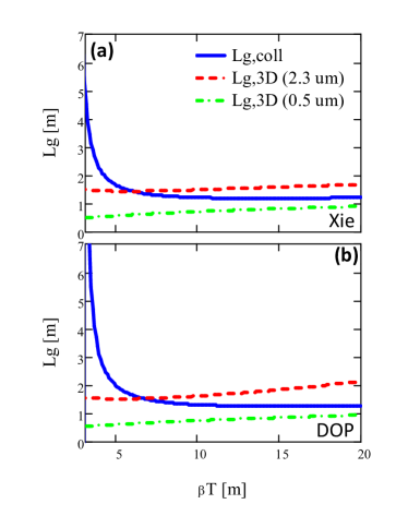
Figure 2: Gain length, calculated with paralmeters listed in Tab.1, as a function of the average Twiss $\beta$ parameter in the undulator according to eq.(23). In (a) $L_{g,3D}$ has been evaluated according to the Xie formalism according to results in (DiMitri2014, ), in (b) the DOP model, used in the present paper, has been considered to evaluate the ihmonogeneous broadening effects on the gain length. Dash green and dot red lines refer to situations when no misaligment is present, in these cases the projected emittance coincides with the slice emittance and $L_{g,coll}$ reduces to $L_{g,3D}$, the two lines are obtained respectively for $\epsilon_{n}=0.5\,mm\,mrad$ and $\epsilon_{n}=2.3\,mm\,mrad$. The blue continuous line refers to $L_{g,coll}$ in presence of a misaligment where the norm. slice emittance $\epsilon_{n}=0.5\,mm\,mrad$ and the norm. projected value is $\epsilon_{n,coll}=2.3\,mm\,mrad$. In all cases the effects of the energy spread have not been considered ($\widetilde{\mu}_{\epsilon}=0)$. It is evident that for small $\beta_{T}$ values an increasing of the gein length occurs, being this conditon of course inauspicious for FEL operation.

The previous identity becomes a measure of $\left\langle x^{\prime 2}\right\rangle$ through the evaluation of the projected emittance. We set

$$\begin{array}[]{l}\left\langle x^{\prime 2}\right\rangle=\Delta\frac{\epsilon}{\beta_{T}}\\ \Delta=\left(\frac{\epsilon_{coll}}{\epsilon}\right)^{2}-1\end{array}$$ (26)

and write $\widetilde{\mu}_{coll}$ as

$$\widetilde{\mu}_{coll}=\frac{\Delta}{\beta_{T}}\frac{\lambda_{u}}{4\pi\sqrt{3}\rho}\frac{\epsilon}{\lambda}$$ (27)

According to the previous identity, large beta values should smear out the detrimental effect of the collective tilt.

The use of the parameter $X$, introduced in eq.(15) allows to cast eq.(27) in the more convenient form

$$\widetilde{\mu}_{coll}=\frac{\Delta}{\beta_{T}^{*}}\frac{\lambda_{u}}{4\pi\sqrt{3}\rho^{*}X^{2/3}}\frac{\epsilon}{\lambda}$$ (28)

The correction to the saturation length foreseen in eq.(23), predicts a critical value of $\beta_{T}$ for which the collective effects are dominating over those associated with those due to the inhomogeneous broadening. This critical value occurs when in eq.(23) $\widetilde{\mu}_{coll}=\zeta^{-1}$, namely when

$$\beta_{ct}=\left[\frac{\Delta}{\zeta\beta_{T}^{*}}L_{g}^{*}\frac{\epsilon}{\lambda}\right]^{3/2}\beta_{T}^{*}$$ (29)

obtained by assuming negligible inhomogeneous effects due to emittance, choosing $\frac{\epsilon}{\lambda}=\frac{1}{4\pi}$ eventually yields

$$\beta_{ct}=\left[\frac{\Delta}{4\pi\zeta\beta_{T}^{*}}L_{g}^{*}\right]^{3/2}\beta_{T}^{*}$$ (30)

In correspondence of this value the saturation length becomes prohibitively long, at least according to the assumption that $\widetilde{\mu}_{coll}$ induced effect are accounted by an equation of the type (23). In Fig.2 we have compared the saturation length vs. $\beta_{T}$ for the the cases corresponding to a normalized slice emittance $\epsilon_{n}$, a normalized projected emittance $\epsilon_{n,coll}$ and to the collective effect with parameters of Tab.1 for the electron beam and radiation. Very similar results are obtained by using the Xie (used also in (DiMitri2014, )) or the DOP formalism to evaluate the 3D corrections to the gain length. The plot axes are limited to a minimum considered $\beta_{T,min}=3$ because (with the assumed parameters for the electron beam) a singulariy occurs, due to the form of eq.(23), for lower $\beta_{T}$ values where the equation is supposed to have no more physical sense. It is worth noting that when $\beta_{T}\gg\beta_{ct}$ the saturation length keeps reasonable values, in between those associated with slice and collective emittance.

IV An alernative point of view

The contribution of the collective effects, using eq.(23), appears as a separate function, appended to the inhomogeneous $\chi$ function and without affecting the other quantities entering the definition of the other $\widetilde{\mu}$ parameters.

A different way of looking at the increasing of the gain length caused by the collective effects, is to leave the same expression as in eqs.(14), but replacing $\varepsilon$ with $\varepsilon_{coll}$ wherever the emittance appears.

Regarding the Pierce parameter and the fact that it is proportional to the cubic root of the beam current density, the correction due to the “collective” emittance yields

$$\begin{array}[]{l}{\rho_{coll}=\rho\left(\frac{\sigma}{\sigma_{coll}}\right)^{\frac{2}{3}}=\rho\left(\frac{\epsilon}{\epsilon_{coll}}\right)^{\frac{1}{3}},}\\ {\sigma_{coll}=\sqrt{\beta_{T}\varepsilon_{coll}}}\end{array}$$ (31)

While as to the inhomogeneous broadening we end up with

$$\begin{array}[]{l}{\tilde{\mu}_{x^{\prime},coll}=\frac{\varepsilon_{coll}}{\beta_{T}}\frac{\gamma^{2}}{\rho_{coll}}\frac{1}{\left(1+\frac{K^{2}}{2}\right)},}\\ {\tilde{\mu}_{x,coll}=\varepsilon_{coll}\frac{\gamma^{2}}{\rho_{coll}}\frac{1}{\left(1+\frac{K^{2}}{2}\right)}\frac{\left(\gamma_{T}^{*}\right)^{2}}{\gamma_{T}},}\\ {\tilde{\mu}_{\varepsilon,coll}=\frac{2\,\sigma_{\varepsilon}}{\rho_{coll}}}\end{array}$$ (32)

It is more convenient to cast them in the form

$$\begin{array}[]{l}{\tilde{\mu}_{x^{\prime},coll}=\tilde{\mu}_{x^{\prime}}\left(\frac{\varepsilon_{coll}}{\varepsilon}\right)^{\frac{5}{3}},}\\ {\tilde{\mu}_{x,coll}=\tilde{\mu}_{x}\left(\frac{\varepsilon_{coll}}{\varepsilon}\right)^{\frac{5}{3}}}\\ {\tilde{\mu}_{\varepsilon,coll}=\tilde{\mu}_{\varepsilon}\left(\frac{\varepsilon_{coll}}{\varepsilon}\right)^{\frac{1}{3}}}\end{array}$$ (33)

which shows that the correction associated with slice misalignment can be characterized by the ratio $\varepsilon_{coll}/\varepsilon$.

With these redefinition of the $\widetilde{\mu}$ parameters, the $\chi$ function of eq.(14) can be rewritten in order to achieve a corrected albeit approximate expression wich includes the collective effects. We can write the function of the $\rho$ depleting formula, and hence the gain length as

$$\frac{L_{g}^{(coll)}}{L_{g}}=\chi_{coll}\cong 1+\left(\frac{\varepsilon_{coll}}{\varepsilon}\right)^{\frac{2}{3}}\left[\left(\tilde{\mu}_{x}^{2}+\tilde{\mu}_{x^{\prime}}^{2}\right)\left(\frac{\varepsilon_{coll}}{\varepsilon}\right)^{\frac{8}{3}}+d\tilde{\mu}_{\varepsilon}^{2}\right]$$ (34)

obtained by neglecting the cross products, where it is also evident the increase of the gain length (hence of the saturation length) at low $\beta_{T}$ values. (34) has been ploted in Fig.3 and compared with a set of numerical simulations, already shown in ref.(DiMitri2014, ) and made with the code GENESIS 1.3 (genesis1.3, ), with good agreement expecially for $\beta_{T}$ values in the reasonable range of operation for an actual FEL with parameters in Tab.1.

In Fig.4 we have plotted the gain length $L_{g}^{(coll)}$ (eq.(34)) vs. the Twiss parameter beta with also including the effect of the energy spread. The results show that the optimum $\beta_{T}$ value depends on the beam qualities. It is worth stressing that in the presence of a larger energy spread the optimization procedure may become critical.

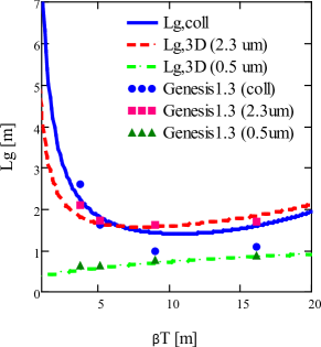
Figure 3: Gain length with the inclusion of the collective effects evaluated from equation (34). Dash green and dot red lines refer to situations when no misaligment is present and respectively for $\epsilon_{n}=0.5\,mm\,mrad$ and $\epsilon_{n}=2.3\,mm\,mrad$. The blue continuous line is the gain length $L_{g}^{(coll)}$with the inclusion of collective effectst with a norm. slice emittance $\epsilon_{n}=0.5\,mm\,mrad$ and a norm. projected value $\epsilon_{n,coll}=2.3\,mm\,mrad$. Energy spread effects are not accounted ($\widetilde{\mu}_{\epsilon}=0)$. The formula fits well with a set of GENESIS 1.3 numerical simulations, described in ref.(DiMitri2014, ), expecially in the region around the minimum $\beta_{T}$ in the optimum range of operation for a FEL with parameters of Tab.1.

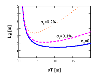
Figure 4: Gain length $L_{g}^{(coll)}$ calculated with paralmeters listed in Tab.1, as a function of the average Twiss $\beta_{T}$ parameter in the undulator, with the inclusion of the effets due to energy spread $\sigma_{\epsilon}=2\rho\widetilde{\mu}_{\epsilon}$. Different lines have been calculated, with a norm. slice emittance $\epsilon_{n}=0.5\,mm\,mrad$ and a norm. collective projected emittance $\epsilon_{n,coll}=2.3\,mm\,mrad$, for different values of the energy spread. Blue continuous, dash purple and dot orange lines are respectively for $\sigma_{\epsilon}=0$, $\sigma_{\epsilon}=0.1\%$ and $\sigma_{\epsilon}=0.2\%$. It is evident, as expected, a deterioration of the beam, and hence an increasing of the gain length, with higher energy spread values.

V Final Comments

In this paper we have addressed the problem of including the increase of the projected emittance growth due to slice misalignment, in the evaluation of the SASE FEL gain. Thus determining the relevant detrimental effects on the saturation length. The key element of the analysis is the introduction of an inhomogeneous broadening like parameter (DiMitri2014, ) which measures the increase of emittance due to collective effects. In order to preserve a line of continuity with the treatment in refs.(MXie, ; SaldinModel, ) it is assumed that this effect has not separated function and affects the saturation length through a suitable redefinition of the Pierce parameter. An effective idea of the interplay between the various detrimental contributions to the the increase of the saturation length is offered by the approximate expression of the $\chi$ function given in eq.(34) which yields an idea of how the various terms due to collective, slice emittances and energy spread contribute to the increase of the gain length. All of the two models indicates that a strong deterioration of the gain length occurs al low values of the matching $\beta_{T}$ Twiss parameter where therefore the operation of the FEL is not convenient. The use of eq.(34) avoids the singularity given by the form of eq.(23). Both parametrization gives also a good agreement with numerical simulations. The choice of one or the other is matter of a careful analysis of the experimental results.

References

- (1) L. Giannessi, Phys. Rev. ST Accel. Beams, 6, 114802 (2003)
- (2) S.G. Biedron et al., Nucl. Instrum. Methods Phys. Res., Sect. A 445, 110-115 (2000)
- (3) M. Xie, Proceedings Particle Accelerator Conference 1995.
- (4) G. Dattoli, T. Letardi, J. M. J. Madey and A. Renieri, J. Quantum Electron 20, 1003 (1984)
- (5) G. Dattoli, A. Renieri, A.Torre and R. Caloi, Nuovo Cimento 11 D, 393-404 (1989)
- (6) G. Dattoli, P.L. Ottaviani, S. Pagnutti, Booklet for FEL design: A collection of practical formulae, Frascati: ENEA–Edizioni Scientifiche, 2007
- (7) E. L. Saldin, E. A. Schneidmiller, and M. V. Yurkov, MOPOS15 in Proceedings of the 26th Free Electron Laser Conference, Trieste, Italy, 2004
- (8) G. Dattoli, A. Renieri and A. Torre, Lectures on The theory of Free Electron Laser and related topics, World Scientific (Singapore) (1993)
- (9) W.B. Colson, C. Pellegrini and A. Renieri. "Classical free electron laser theory." Laser Handbook 6.115: 75 (1990).
- (10) T. Tanaka, H. Kitamura, T. Shintake, Nucl. Instrum. Methods Phys. Res., Sect. A 528, 172-178 (2004)
- (11) G. Dattoli, L. Giannessi, P.L. Ottaviani, C. Ronsivalle, Journal of Applied Physics, 95(6), 3206 (2004)
- (12) G. Dattoli, E. Sabia, C. Ronsivalle, M. Del Franco, A. Petralia, Nuclear Instr. and Methods A 671, 51-61 (2012)
- (13) S. DI Mitri, S. Spampinati, Phys Rev. ST Accel. Beams 17, 110702 (2014)
- (14) M.W. Guetg et al., Phys Rev. ST Accel. Beams 18, 030701 (2015)
- (15) M. Quattromini, M. Artioli, E. Di Palma, A. Petralia, and L. Giannessi Phys. Rev. ST Accel. Beams 15, 080704 (2012)
- (16) S. Reiche et al., Nucl. Instrum. Methods Phys. Res., Sect. A 429, 243 (1999).