On the geometry of Stein variational gradient descent

Abstract

Bayesian inference problems require sampling or approximating high-dimensional probability distributions. The focus of this paper is on the recently introduced Stein variational gradient descent methodology, a class of algorithms that rely on iterated steepest descent steps with respect to a reproducing kernel Hilbert space norm. This construction leads to interacting particle systems, the mean-field limit of which is a gradient flow on the space of probability distributions equipped with a certain geometrical structure. We leverage this viewpoint to shed some light on the convergence properties of the algorithm, in particular addressing the problem of choosing a suitable positive definite kernel function. Our analysis leads us to considering certain nondifferentiable kernels with adjusted tails. We demonstrate significant performance gains of these in various numerical experiments.

Keywords: Bayesian inference, gradient flows, geometry of optimal transport, Stein’s method, reproducing kernel Hilbert spaces

1 Introduction

Sampling and Variational Inference (VI) are the most common paradigms for extracting information from posterior distributions arising from Bayesian inference problems. This is a particularly challenging problem in high dimensions, where the posterior distribution will only be known up to a constant of normalisation. Markov Chain Monte Carlo (MCMC) methods based on the Metropolis-Hastings algorithm provide a generic approach to sampling from such distributions. However, in high dimensions these methods suffer from poor scalability due to correlation between successive samples. Variational techniques reformulate inference as an optimisation problem; seeking a distribution from a family of simple probability distributions which best approximates the target posterior distribution. VI typically permits faster inference, albeit at the cost of losing asymptotic exactness.

Recently there has been interest in particle optimisation techniques which combine aspects of both approaches. Here, an ensemble of particles are collectively evolved forward, seeking to approximate the posterior distribution. One such approach, known as Stein Variational Gradient Descent (SVGD), was introduced in Liu and Wang (2016). In this method, an ensemble of $N$ particles in $\mathbb{R}^{d}$ defining an empirical measure $\rho^{N}$ is moved forward in a series of discrete steps via the map

$$x\mapsto T(x)=x+\varepsilon\psi(x),$$

where $\varepsilon$ is the step size and $\psi$ is a vector field, which is chosen such that the pushforward measure $T_{\sharp}\rho^{N}$ has minimal KL divergence with respect to the target posterior $\pi\propto\exp(-V)$. Choosing $\psi$ from within the unit ball of a vector valued RKHS $\mathcal{H}_{k}^{d}$ with positive definite kernel $k:\mathbb{R}^{d}\times\mathbb{R}^{d}\rightarrow\mathbb{R}$ results in discrete dynamics of the form

$$X^{i}_{n+1}=X^{i}_{n}-\frac{\varepsilon}{N}\left(\sum_{j=1}^{N}\nabla k(X^{i}_{n},X^{j}_{n})+\sum_{j=1}^{N}k(X^{i}_{n},X^{j}_{n})\nabla V(X^{j}_{n})\right),$$

where $\nabla k$ denotes the gradient with respect to the first variable. In the continuous time limit, as $\varepsilon\rightarrow 0$, this results in the following system of ordinary differential equations (ODEs) describing the evolution of the particles $X^{1},\ldots,X^{N}$,

$$\frac{\mathrm{d}X_{t}^{i}}{\mathrm{d}t}=-\frac{1}{N}\sum_{j=1}^{N}\nabla k(X_{t}^{i},X_{t}^{j})-\frac{1}{N}\sum_{j=1}^{N}k(X_{t}^{i},X_{t}^{j})\nabla V(X_{t}^{j}),\quad i=1,\ldots,N.$$ (1)

It was observed in Liu (2017) that the scaling limit of (1) as $N\rightarrow\infty$ is given by the mean-field equation

$$\partial_{t}\rho_{t}(x)=\nabla\cdot\left(\rho_{t}(x)\int_{\mathbb{R}^{d}}k(x,y)\left[\nabla\rho_{t}(y)+\rho_{t}(y)\nabla V(y)\right]\mathrm{d}y\right),$$ (2)

where $\rho$ denotes the limiting density of the particles as $N$ tends to infinity. The convergence of $\rho^{N}$ to $\rho$ was proved rigorously in Lu et al. (2019a) together with existence and uniqueness for (2), as well as convergence to equilibrium, albeit without quantitative rates. In Liu (2017) it was observed that the evolution equation (2) can be viewed as a gradient flow on the space of probability densities, equipped with a certain distance that depends on the kernel $k$. Remarkably, this observation places SVGD in direct correspondence with the more conventional (overdamped) Langevin dynamics (Pavliotis, 2014), see Appendix A. Our main focus in this paper is to follow the thread of this parallel and leverage the gradient flow perspective for the study of contraction and equilibration properties of (2). To wit, we develop a second order calculus and study the convexity properties of the $\mathrm{KL}$-divergence with respect to an appropriately constructed geometry on the space of probability densities, henceforth called Stein geometry, and identify conditions in the form of functional inequalities which are necessary for exponential convergence of $\rho_{t}$ to the equilibrium $\pi$. Building on this analysis, we are able to derive principled guidelines for making a suitable choice of the kernel function $k$. In particular, we explore analytically and numerically the use of singular kernel functions, i.e. those that are not continuously differentiable. In our experiments we demonstrate significant performance gains in a variety of inference tasks.

1.1 Previous work

The SVGD method has attracted a lot of interest since it was introduced in Liu and Wang (2016). Indeed, numerous variants have been proposed which improve scalability by exploiting additional information such as the conditional dependency structure (Zhuo et al., 2018) or the underlying geometry of the posterior (Chen et al., 2019; Detommaso et al., 2018; Liu and Zhu, 2018; Wang et al., 2019a). Stochastic variants which introduce noise into the dynamics in order to aid exploration and efficiency of SVGD have also been proposed (Gallego and Insua, 2018; Li et al., 2020; Zhang et al., 2020, 2018). Other methods in the spirit of particle optimisation have been proposed, such as Ambrogioni et al. (2018); Bigoni et al. (2019); Chen et al. (2018b); Liu et al. (2019); Mroueh et al. (2018, 2019). The potential of SVGD has also been explored in the context of sequentially updated Bayesian posteriors (Detommaso et al., 2019; Pulido and van Leeuwen, 2018).

Gradient flows provide a natural formalism in which to analyse the long-term behaviour of certain classes of nonlinear, nonlocal partial differential equations with dissipative behaviour. This includes many PDEs arising as the mean-field equations of ensembles of interacting stochastic particle systems.

The space of densities equipped with the quadratic Wasserstein metric formally defines a Riemannian structure over which gradient flows can be defined. It is well known that solutions to the Fokker-Plank equation associated with the overdamped Langevin dynamics can be formulated as gradient flows of the $\mathrm{KL}$-divergence (or relative entropy) with respect to the Wasserstein metric. Analysis of the geodesic convexity of the $\mathrm{KL}$-divergence yields conditions under which exponential convergence to equilibrium can be established. This differential-geometric perspective was put forward by F. Otto and coworkers (see for example Jordan et al. (1998); Otto (2001); Otto and Westdickenberg (2005) or Villani (2009, Chapter 15) and Villani (2003a, Chapter 9)). Of particular importance for the development in Section 5 is the discussion in Otto and Villani (2000, Section 3). Extensions to systems of overdamped Langevin particles with various forms of interactions and their relationships to ensemble Kalman filters and inverse problems (Iglesias et al., 2013) have also been considered (Garbuno-Inigo et al., 2020a, b; Nüsken and Reich, 2019), see also the extension to $\gamma$-drift diffusions studied in Li (2019). In Lu et al. (2019b), the Langevin dynamics are augmented with interactions giving rise to a nonlocal birth-death term in the mean-field equations. By reformulating the system as a gradient flow of the $\mathrm{KL}$-divergence with respect to the Wasserstein-Fisher-Rao metric, sufficient conditions for expontential convergence to equilibrium are obtained with quantitative rates. The dynamics put forward in Pathiraja and Reich (2019); Reich and Weissmann (2021) are based on approximations of the particle-density within a suitably chosen RKHS; this approach should be contrasted with SVGD which relies on a driving vector field with minimal RKHS-norm. We would also like to refer the reader to Wang and Li (2020), where Newton gradient flows have been developed, holding the promise of accelerating convergence in the face of ill-conditioning.

In the context of machine learning a number of recent works have proposed gradient flow formulations of methods for sampling and variational inference, see for example Arbel et al. (2019); Li and Montúfar (2018); Lu et al. (2019b); Wang et al. (2019b); Gao et al. (2019); Li and Montúfar (2020). In particular, a number of approaches which unify Langevin dynamics and SVGD via the common framework of Wasserstein gradient flows have also appeared (Chen and Zhang, 2017; Chen et al., 2018a).

1.2 Our contribution

The contributions in this paper are:

• Following Liu (2017) we formulate the mean-field limit of SVGD as a gradient flow of the $\mathrm{KL}$-divergence in the so-called Stein geometry. We define appropriate tangent spaces and study foundational properties of the structure thus obtained.

• We derive expressions for the geodesics in this geometry and based on these, explore second order properties of the gradient flow dynamics. The latter are intimately related to a qualitative and quantitative understanding of the convergence to equilibrium, as has been widely recognised in the literature on Wasserstein gradient flows (see Villani (2009) and references therein). By way of counterexample, we show that, within this framework and using only entropy as the driving force, it is in general impossible to obtain bounds on the Stein-Hessian operator that would allow us to conclude exponential convergence as in the Wasserstein case.

• Moreover, we study the curvature of the $\mathrm{KL}$-divergence around equilibrium, and identify conditions in the form of functional inequalities which are equivalent to exponential decay when near equilibrium. In certain scenarios we show that there is a direct correspondence with functional-analytic properties of the reproducing kernel Hilbert space (RKHS) associated to the kernel function $k$.

• Based on this we derive a series of guidelines for making a suitable choice of kernel function $k$, especially placing emphasis on regularity and tail properties.

We would like to point out that differential-geometric tools at this point mainly serve for intuition, and that a rigorous formulation in the framework of metric length spaces has been carried out in Ambrosio et al. (2008) for the Wasserstein case. Adapting those techniques to the Stein geometry is an interesting direction for future work.

The remainder of the paper will be as follows. In Section 2 we shall introduce basic notation and a number of preliminary assumptions. In Section 3 we discuss a stochastic variant of the SVGD dynamics (originally proposed in Gallego and Insua (2018)) and show that the resulting mean-field PDE coincides with (2). In Section 4 we recall and extend the Stein geometry introduced in Liu (2017), in particular characterising the solution of the mean-field equation (2) as a gradient flow of the $\mathrm{KL}$-divergence with respect to this geometry. In Section 5 we study the geodesic equations under the Stein metric and investigate the geodesic convexity of the $\mathrm{KL}$-divergence. In Section 6 we focus on the long-time behaviour when close to equilibrium, and in particular identify conditions in the form of functional inequalities for exponential return. In Section 7 we give a brief outlook at applications of the developed theory for polynomial kernels. In Section 8 a number of numerical experiments are presented to confirm and complement the theory. Comments and conclusions are deferred to Section 9. In Appendix A we draw parallels between SVGD and the Stein geometry on the one hand, and Langevin dynamics and the Wasserstein geometry on the other hand.

2 Assumptions and Preliminaries

2.1 Notation and preliminaries

We first briefly define the function spaces which will be used throughout this paper. The space $C_{c}^{\infty}(\mathbb{R}^{d})$ consists of smooth functions with compact support, and $\mathcal{D}^{\prime}(\mathbb{R}^{d})$ refers to its topological dual, the space of distributions. Given a probability measure $\rho$ on $\mathbb{R}^{d}$ we define $L^{2}(\rho)$ to be the Hilbert space of square-integrable functions with respect to $\rho$ with inner product $\langle\phi,\psi\rangle_{L^{2}(\rho)}=\int_{\mathbb{R}^{d}}\phi\psi\,\mathrm{d}\rho$. The subspace $L_{0}^{2}(\rho)$ consists of centered functions in $L^{2}(\rho)$, that is,

$$L_{0}^{2}(\rho)=\left\{\phi\in L^{2}(\rho):\quad\int_{\mathbb{R}^{d}}\phi\,\mathrm{d}\rho=0\right\}.$$ (3)

We define the (weighted) Sobolev space $H^{1}(\rho)$ to be the subspace of $L^{2}(\rho)$ functions having derivatives also in $L^{2}(\rho)$, i.e.

$$H^{1}(\rho)=\left\{\phi\in L^{2}(\rho):\quad\|\nabla\phi\|_{L^{2}(\rho)}<\infty\right\}.$$

The following assumption on $k$ is fundamental:

Assumption 1 (Assumptions on $k$)

The kernel $k:\mathbb{R}^{d}\times\mathbb{R}^{d}\rightarrow\mathbb{R}$ is continuous, symmetric and positive definite, i.e.

$$\sum_{i,j=1}^{n}\alpha_{i}\alpha_{j}k(x_{i},x_{j})\geq 0,$$

for all $n\in\mathbb{N}$, $\alpha_{1},\ldots\alpha_{n}\in\mathbb{R}$ and $x_{1},\ldots,x_{n}\in\mathbb{R}^{d}$.

Canonical examples of kernels satisfying Assumption 1 include the Gaussian kernel $k(x,y)=\exp\left(-\frac{|x-y|^{2}}{\sigma^{2}}\right)$, and Laplace kernel $k(x,y)=\exp\left(-\frac{|x-y|}{\sigma}\right)$. More generally, we will consider the kernels $k_{p,\sigma}:\mathbb{R}^{d}\times\mathbb{R}^{d}\rightarrow\mathbb{R}$, defined via

$$k_{p,\sigma}(x,y)=\exp\left(-\frac{|x-y|^{p}}{\sigma^{p}}\right),$$ (4)

where $p\in(0,2]$ is a smoothness parameter, and $\sigma>0$ is called the kernel width.

Let $(\mathcal{H}_{k},\langle\cdot,\cdot\rangle_{\mathcal{H}_{k}})$ be the reproducing kernel Hilbert space (RKHS) associated to the kernel $k$, (Steinwart and Christmann, 2008, Sec 4.2), that is, $\mathcal{H}_{k}$ is the Hilbert space of all functions on $\mathbb{R}^{d}$ such that, for $x\in\mathbb{R}^{d}$, $k(x,\cdot)\in\mathcal{H}_{k}$ and $f(x)=\langle f,k(x,\cdot)\rangle_{\mathcal{H}_{k}}$. We let $\|\cdot\|_{\mathcal{H}_{k}}$ be the norm induced by the inner product on $\mathcal{H}_{k}$. The $d$-fold Cartesian product

$$\mathcal{H}^{d}_{k}=\underbrace{\mathcal{H}_{k}\times\ldots\times\mathcal{H}_{k}}_{d\,\text{times}}$$ (5)

is a Hilbert space of vector fields $v=(v_{1},\ldots,v_{d}):\mathbb{R}^{d}\rightarrow\mathbb{R}^{d}$, equipped with the norm

$$\|v\|_{\mathcal{H}_{k}^{d}}^{2}=\sum_{i=1}^{d}\|v_{i}\|^{2}_{\mathcal{H}_{k}}.$$

Remark 1 (Vector-valued RKHS)

More generally one can consider matrix-valued kernels of the form $\bar{k}:\mathbb{R}^{d}\times\mathbb{R}^{d}\rightarrow\mathbb{R}^{d\times d}$, (Carmeli et al., 2006; Micchelli and Pontil, 2005), as has recently been done in Wang et al. (2019a). The associated RKHS $\mathcal{H}_{\bar{k}}$ then consists of vector-valued functions. We leave the analysis of SVGD algorithms based on matrix-valued kernels for future work.

The following is a nondegeneracy assumption on $k$, instrumental in guaranteeing convergence of solutions to (2) towards the target $\pi$.

Assumption 2

(Fukumizu et al., 2009; Sriperumbudur et al., 2010) The kernel $k$ is integrally strictly positive definite (ISPD), i.e.

$$\int_{\mathbb{R}^{d}}\int_{\mathbb{R}^{d}}k(x,y)\,\mathrm{d}\rho(x)\mathrm{d}\rho(y)>0$$

holds for all finite nonzero signed Borel measures $\rho$.

From Sriperumbudur et al. (2010, Theorem 7), ISPD kernels are characteristic, i.e. the kernel mean embedding $\rho\mapsto\int k(\cdot,y)\,\mathrm{d}\rho(y)$ is injective. We note that the kernels defined in (4) (in particular, the Gauss and Laplace kernels) are ISDP, see Lemma 44 below.

Throughout this article, we will denote by $\mathcal{P}(\mathbb{R}^{d})$ the space of probability measures on $\mathbb{R}^{d}$. Abusing the notation, we will use the same letter for their Lebesgue densities in case they exist. Given a kernel $k$, we define the following subset of $\mathcal{P}(\mathbb{R}^{d})$,

$$\mathcal{P}_{k}(\mathbb{R}^{d})=\Bigg{\{}\rho\in\mathcal{P}(\mathbb{R}^{d}):\quad \rho\,\,\text{admits a smooth Lebesgue density,}\quad\operatorname{supp}\rho=\mathbb{R}^{d},$$

$$\quad\int_{\mathbb{R}^{d}}k(x,x)\,\mathrm{d}\rho(x)<\infty\Bigg{\}},$$

and, for $\rho\in\mathcal{P}_{k}(\mathbb{R}^{d})$, the linear operator $\mathcal{T}_{k,\rho}:L^{2}(\rho)\rightarrow\mathcal{H}_{k}$ via

$$\mathcal{T}_{k,\rho}\phi=\int_{\mathbb{R}^{d}}k(\cdot,y)\phi(y)\,\mathrm{d}\rho(y),\quad\phi\in L^{2}(\rho).$$ (7)

For $\rho\in\mathcal{P}_{k}(\mathbb{R}^{d})$, $\mathcal{T}_{k,\rho}$ is compact, self-adjoint and positive semi-definite. Furthermore, by Steinwart and Christmann (2008, Theorem 4.26) the associated RKHS $\mathcal{H}_{k}$ will consist of $L^{2}(\rho)$-functions. By Assumption 2 and the fact that $\operatorname{supp}\rho=\mathbb{R}^{d}$, $\mathcal{T}_{k,\rho}$ is injective, and consequently, the embedding $\mathcal{H}_{k}\subset L^{2}(\rho)$ is dense. For a normed vector space $V$ (such as $L^{2}(\rho)$, $H^{1}(\rho)$ or $\mathcal{H}_{k}$ above) and a subset $A\subset V$, we denote by $\overline{A}^{V}\subset V$ the closure in the corresponding norm. That is, $\overline{A}^{V}$ is the smallest set containing $A$ that is closed with respect to $\|\cdot\|_{V}$.

Finally, our objective will be to generate samples from the target density $\pi\propto e^{-V}$ on $\mathbb{R}^{d}$. We shall make the following basic assumptions on $\pi$ and $V$:

Assumption 3

The potential $V:\mathbb{R}^{d}\rightarrow\mathbb{R}$ is continuously differentiable, with $e^{-V}\in L^{1}(\mathbb{R}^{d})$. The target density is given by

$$\pi=\frac{1}{Z}e^{-V},$$ (8)

where $Z=\int_{\mathbb{R}^{d}}e^{-V}\mathrm{d}x$ is the normalising constant. Furthermore, $\pi\in\mathcal{P}_{k}(\mathbb{R}^{d})$.

3 Stochastic SVGD and its Mean Field Limit

Before turning our focus towards the main topic of this paper in Section 4, we comment on a stochastic variant of (1), providing another link to the overdamped Langevin dynamics. This section can be skipped (or read independently from the rest of the paper). The follow-up work Nüsken and Renger (2021) connects the deterministic dynamics (1) to its stochastic augmentation (9) discussed below using the theory of large deviations and the geometric framework developed in this paper.

In Gallego and Insua (2018), the following modification of (1) was introduced,

$$\mathrm{d}\bar{X}_{t}=\left(-\mathcal{K}(\bar{X}_{t})\nabla\bar{V}(\bar{X}_{t})+\nabla\cdot\mathcal{K}(\bar{X}_{t})\right)\mathrm{d}t+\sqrt{2\mathcal{K}(\bar{X}_{t})}\,\mathrm{d}W_{t},$$ (9)

where $\bar{X}=(X^{1},\ldots,X^{N})\in\mathbb{R}^{Nd}$ comprises the collection of particles, $(W_{t})_{t\geq 0}$ denotes an $Nd$-dimensional standard Brownian motion,

$$\bar{V}(x_{1},\ldots,x_{N})=\sum_{i=1}^{N}V(x_{i})$$

is the extended potential, and the state-dependent mass matrix $\mathcal{K}:\mathbb{R}^{Nd}\rightarrow\mathbb{R}^{Nd\times Nd}$ can be decomposed into $N^{2}$ blocks of size $d\times d$ as follows,

$$\mathcal{K}(\bar{x})=\begin{pmatrix}{K}_{11}(\bar{x})&\dots&K_{1N}(\bar{x})\\ \vdots&\ddots&\vdots\\ K_{N1}(\bar{x})&\ldots&K_{NN}(\bar{x})\end{pmatrix},$$

where

$$K_{ij}(\bar{x})=\frac{1}{N}k(x_{i},x_{j})I_{d\times d}.$$

Furthermore, $\sqrt{\mathcal{K}(\bar{x})}$ denotes a square root of the nonnegative matrix $\mathcal{K}(\bar{x})$. By definition,

$$(\nabla\cdot\mathcal{K})_{i}=\sum_{j=1}^{Nd}\frac{\partial\mathcal{K}_{ij}}{\partial\bar{x}_{j}},\qquad i=1,\ldots,Nd,$$

so we see that the $i^{th}$ coordinate $X_{t}^{i}$ satisfies the SDE

$$\mathrm{d}X_{t}^{i}=\frac{1}{N}\sum_{j=1}^{N}\left[-k(X_{t}^{i},X_{t}^{j})\nabla V(X_{t}^{j})+\nabla_{X_{t}^{j}}k(X_{t}^{i},X_{t}^{j})\right]\mathrm{d}t+\sum_{j=1}^{N}\sqrt{2\mathcal{K}(\bar{X}_{t})}_{ij}\,\mathrm{d}W_{t}^{j},$$ (10)

coinciding with (1) up to the noise term $\sqrt{2\mathcal{K}(\bar{X}_{t})}\,\mathrm{d}W_{t}$. Indeed, this perturbation becomes vanishingly small in the limit as $N\rightarrow\infty$, and the mean-field limits of (1) and (9) agree:

Proposition 2 (Formal identification of the mean-field limit)

As $N\rightarrow\infty$, the empirical measure $\rho_{t}^{N}=\frac{1}{N}\sum_{i=1}^{N}\delta_{X_{t}^{i}}$ associated with (10) converges to the solution $\rho_{t}$ of (2).

Proof  See Appendix B.  
It is straightforward to check that

$$\bar{\pi}(x_{1},\ldots,x_{N}):=\prod_{i=1}^{N}\pi(x_{i})=\frac{1}{Z^{N}}\exp\left(-\sum_{i=1}^{N}V(x_{i})\right)$$ (11)

is an invariant probability density for (9), with marginals

$$\int_{\mathbb{R}^{(N-1)d}}\bar{\pi}(x_{1},\ldots,x_{N})\,\mathrm{d}x_{1}\ldots\widehat{\mathrm{d}x_{i}}\ldots\mathrm{d}x_{N}=\pi(x_{i}).$$

Below, we will show that under mild conditions, the dynamics (9) is in fact ergodic with respect to $\bar{\pi}$, so that in particular

$$\frac{1}{T}\int_{0}^{T}\frac{1}{N}\sum_{i=1}^{N}\phi(X_{t}^{i})\,\mathrm{d}t\xrightarrow{T\rightarrow\infty}\int_{\mathbb{R}^{d}}\phi\,\mathrm{d}\pi,\quad\text{a.s.},$$ (12)

for any test function $\phi\in C_{b}(\mathbb{R}^{d})$. Suitable discretisations of (9) therefore lead to MCMC-type algorithms on an extended state space in the framework of Ma et al. (2015), as already noticed in Gallego and Insua (2018). See also Duncan et al. (2017, Section 2.2) and Nüsken and Pavliotis (2019) for related discussions.

For our ergodicity result we need the following set of assumptions:

Assumption 4

The following hold:

1. The SDE (9) admits a global strong solution.

2. We have $\mathbb{E}\int_{0}^{t}|\nabla V(X^{i}_{s})|\,\mathrm{d}s<\infty$ for all $i=1,\ldots,N$ and all $t>0$.

3. The kernel $k$ is translation-invariant, i.e.

   $$k(x,y)=h\left(x-y\right),\quad x,y\in\mathbb{R}^{d},$$

   where $h\in C(\mathbb{R}^{d})\cap C^{1}(\mathbb{R}^{d}\setminus\{0\})$ is Lipschitz continuous, and its gradient satisfies the one-sided Lipschitz condition

   $$\left(\nabla h(x)-\nabla h(y)\right)\cdot(x-y)\leq C|x-y|^{2},$$ (13)

   for some constant $C$ and all $x,y\neq 0$.

Proposition 3 (Ergodicity of stochastic SVGD)

Let Assumption 4 be satisfied, $d\geq 2$, and assume that the initial condition for (10) is distinct, i.e. $X_{0}^{i}\neq X_{0}^{j}$ for $i\neq j$. Then $X_{t}^{i}\neq X_{t}^{j}$ for $i\neq j$ for all $t>0$, almost surely. Moreover, the process $(\bar{X}_{t})_{t\geq 0}$ is ergodic with respect to the product measure (11).

Proof  See Appendix B.  

Remark 4

Assumption 4.2 holds under suitable (mild) conditions on the growth of $V$ at infinity. Any bounded translation-invariant kernel of regularity $C^{2}$ satisfies Assumption 4, (3). Specifically, the kernels (4) satisfy Assumption 4.3 if $p\in[1,2]$. In the case when $p<1$ these kernels are not Lipschitz continuous. We leave an extension of Proposition 3 to this regime for future work. Note that the assumption of translation-invariance can easily be weakened, but we choose to impose it for ease of presentation.

4 SVGD as a gradient flow

In Liu (2017) it was observed that the evolution equation (2) can be interpreted as gradient flow dynamics of the $\mathrm{KL}$-divergence on the space of probability measures equipped with a novel distance $d_{k}$ that depends on the chosen kernel. Formally, $d_{k}$ is furthermore the geodesic distance induced by a suitably chosen Riemannian metric. Here we review this perspective and identify the relevant tangent spaces, preparing the ground for our calculations in the later sections. Let us remark that in order to understand the results of the later sections Corollary 13 suffices; the remainder of this section may thus be skipped at first reading.

In what follows we set up a formal Riemannian calculus on $\mathcal{P}_{k}(\mathbb{R}^{d})$, acting as though $\mathcal{P}_{k}(\mathbb{R}^{d})$ was a smooth manifold. To reinforce this heuristic viewpoint, and for notational convenience, we will use the shorthand $M:=\mathcal{P}_{k}(\mathbb{R}^{d})$. This perspective (nowadays known as Otto calculus) has been put forward for the case of the quadratic Wasserstein distance in the seminal works Jordan et al. (1998); Otto (1998, 2001); Otto and Villani (2000); Otto and Westdickenberg (2005) and was further developed in Ambrosio et al. (2008); Gigli (2012) and Daneri and Savaré (2008). For textbook accounts we refer to Villani (2003a, Chapter 8), Villani (2009, Chapter 15) and Ambrosio and Gigli (2013, Chapter 3).

To facilitate intuition, we begin with an informal discussion. Speaking in broad terms, many particle-based methods in general (see Section 1.1), and SVGD in particular, postulate dynamical schemes of the form

$$\frac{\mathrm{d}X_{t}}{\mathrm{d}t}=v_{t}(X_{t}),\qquad X_{0}\sim\rho_{0}.$$ (14)

Those are based on a family of vector fields $v_{t}$, inducing a flow of probability measures $\rho_{t}=\operatorname{Law}X_{t}$. Under mild growth and regularity assumptions on $v_{t}$, the evolution of $\rho_{t}$ is governed by the continuity equation

$$\partial_{t}\rho_{t}+\nabla\cdot(\rho_{t}v_{t})=0,$$ (15)

see, for instance, Ambrosio and Gigli (2013, Section 4.1.2). On the other hand, given a flow of probability measures $\rho_{t}$, we may reverse this logic and ask for a family of vector fields $v_{t}$ that reproduces $\rho_{t}$, in the sense of (15), or, equivalently, (14). Notice that $v_{t}$ will not be unique, since for any sufficiently regular density $\rho_{t}$ there exist infinitely many vector fields $u_{t}$ that satisfy $\nabla\cdot(\rho_{t}u_{t})=0$; those $u_{t}$ can be added to any $v_{t}$ without affecting the validity of (15). To enforce uniqueness, it is reasonable to either select $v_{t}$ so as to minimise a certain norm or to constrain it to lie in a specified subspace (while at the same time satisfying (15)). The following result shows that requiring $v_{t}$ to have minimal $\mathcal{H}_{k}^{d}$-norm is equivalent to $v_{t}\in\overline{\mathcal{T}_{k,\rho_{t}}\nabla C_{c}^{\infty}(\mathbb{R}^{d})}^{\mathcal{H}_{k}^{d}}$, that is, up to taking limits in $\mathcal{H}_{k}^{d}$, $v_{t}$ is a gradient field, convolved using the operator $\mathcal{T}_{k,\rho}$ defined in (7). In other words, the SVGD construction principle originally put forward in Liu and Wang (2016) (namely to construct movement schemes that are minimal in $\mathcal{H}_{k}^{d}$-sense) implies that $v_{t}\in\overline{\mathcal{T}_{k,\rho_{t}}\nabla C_{c}^{\infty}(\mathbb{R}^{d})}^{\mathcal{H}_{k}^{d}}$ for dynamics of the form (14).

Proposition 5 (Selection principle)

Let the pair $(\rho,v):(0,1)\rightarrow\mathcal{P}_{k}(\mathbb{R}^{d})\times\mathcal{H}_{k}^{d}$ satisfy the continuity equation (15). Furthermore, assume that $v_{t}\in\overline{\mathcal{T}_{k,\rho_{t}}\nabla C_{c}^{\infty}(\mathbb{R}^{d})}^{\mathcal{H}_{k}^{d}}$, for all $t\in(0,1)$. Then the following hold:

1. Given $\rho$, the vector field $v$ is the unique solution to (15) in $\overline{\mathcal{T}_{k,\rho_{t}}\nabla C_{c}^{\infty}(\mathbb{R}^{d})}^{\mathcal{H}_{k}^{d}}$: If $(\rho,w):(0,1)\rightarrow\mathcal{P}_{k}(\mathbb{R}^{d})\times\mathcal{H}_{k}^{d}$ also satisfies (15) as well as $w_{t}\in\overline{\mathcal{T}_{k,\rho_{t}}\nabla C_{c}^{\infty}(\mathbb{R}^{d})}^{\mathcal{H}_{k}^{d}}$ for all $t\in(0,1)$, then $v=w$.

2. The vector field $v$ minimises the $\mathcal{H}_{k}^{d}$-norm among solutions to (15): Let $w:(0,1)\rightarrow\mathcal{H}_{k}^{d}$ be any other vector field that together with $\rho$ satisfies (15). Then

   $$\|v_{t}\|_{\mathcal{H}_{k}^{d}}\leq\|w_{t}\|_{\mathcal{H}_{k}^{d}},\qquad\qquad\text{for all }t\in(0,1).$$

The following proposition (proven in Appendix C) provides the basis for Proposition 5, as well as for many of the other constructions in this section. It should be compared to the usual $L^{2}(\rho)$-orthogonal decomposition of vectors fields into gradients and (weighted) divergence-free vector fields, see, for instance, Figalli and Glaudo (2021).

Proposition 6 (Helmholtz decomposition for RKHS)

Let $\rho\in M$ and define the space of (weighted) divergence-free vector fields

$$L^{2}_{\mathrm{div}}(\rho)=\left\{v\in(L^{2}(\rho))^{d}:\quad\langle v,\nabla\phi\rangle_{(L^{2}(\rho))^{d}}=0,\quad\text{for all }\phi\in C_{c}^{\infty}(\mathbb{R}^{d})\right\}.$$

Then $\mathcal{H}_{k}^{d}$ admits the following $\langle\cdot,\cdot\rangle_{\mathcal{H}^{d}_{k}}$-orthogonal decomposition,

$$\mathcal{H}_{k}^{d}=\left(L^{2}_{\mathrm{div}}(\rho)\cap\mathcal{H}_{k}^{d}\right)\oplus\overline{\mathcal{T}_{k,\rho}\nabla C_{c}^{\infty}(\mathbb{R}^{d})}^{\mathcal{H}_{k}^{d}}.$$

Proof of Proposition 5 For the first claim, notice that $\nabla\cdot(\rho_{t}(v_{t}-w_{t})))=0$, for all $t\in(0,1)$. Since also $v_{t}-w_{t}\in\overline{\mathcal{T}_{k,\rho_{t}}\nabla C_{c}^{\infty}(\mathbb{R}^{d})}^{\mathcal{H}_{k}^{d}}$, the statement follows directly from the Helmholtz decomposition for $\mathcal{H}_{k}^{d}$ in Proposition 6. For the second claim, notice that we can decompose $w_{t}=v_{t}+u_{t}$, where $\nabla\cdot(\rho_{t}u_{t})=0$. From the orthogonality in (16) it then follows that

$$\|w_{t}\|^{2}_{\mathcal{H}_{k}^{d}}=\|v_{t}\|^{2}_{\mathcal{H}_{k}^{d}}+\underbrace{2\langle v_{t},u_{t}\rangle_{\mathcal{H}_{k}^{d}}}_{=0}+\|u_{t}\|^{2}_{\mathcal{H}_{k}^{d}}\geq\|v_{t}\|^{2}_{\mathcal{H}_{k}^{d}},$$ (16)

as required.  

After this intuitive introduction, we proceed by introducing a suitable notion of tangent spaces equipped with positive-definite quadratic forms, playing the role of Riemannian metrics. This construction is motivated by the special role played by the spaces $\overline{\mathcal{T}_{k,\rho}\nabla C_{c}^{\infty}(\mathbb{R}^{d})}^{\mathcal{H}_{k}^{d}}$ according to Proposition 5 and justified by Corollary 13 (see below). We follow Mielke et al. (2014, Section 4.2) in style of exposition.

Definition 7 (Tangent spaces and Riemannian metric)

For $\rho\in M$, we define the tangent space

$$T_{\rho}M=\Bigg{\{}\xi\in\mathcal{D}^{\prime}(\mathbb{R}^{d}):\quad \text{there exists }v\in\overline{\mathcal{T}_{k,\rho}\nabla C_{c}^{\infty}(\mathbb{R}^{d})}^{\mathcal{H}_{k}^{d}}\,\,\text{such that}$$ (17a)

$$\xi+\nabla\cdot(\rho v)=0\quad\text{in the sense of distributions}\Bigg{\}}$$ (17b)

and the Riemannian metric $g_{\rho}:T_{\rho}M\times T_{\rho}M\rightarrow\mathbb{R}$ by

$$g_{\rho}(\xi,\chi)=\langle u,v\rangle_{\mathcal{H}_{k}^{d}},$$ (18)

where $\xi+\nabla\cdot(\rho u)=0$ and $\chi+\nabla\cdot(\rho v)=0$.

Remark 8

As usual, we say that $\xi+\nabla\cdot(\rho v)=0$ holds in the sense of distributions if

$$\langle\xi,\phi\rangle-\int_{\mathbb{R}^{d}}\nabla\phi\cdot v\,\mathrm{d}\rho=0,$$

for all $\phi\in C_{c}^{\infty}(\mathbb{R}^{d})$, where $\langle\cdot,\cdot\rangle$ denotes the duality pairing between $\mathcal{D}^{\prime}(\mathbb{R}^{d})$ and $C_{c}^{\infty}(\mathbb{R}^{d})$. Moreover, $\overline{\mathcal{T}_{k,\rho}\nabla C_{c}^{\infty}(\mathbb{R}^{d})}^{\mathcal{H}_{k}^{d}}$ refers to the closure of the set $\mathcal{T}_{k,\rho}\nabla C_{c}^{\infty}(\mathbb{R}^{d})=\left\{\mathcal{T}_{k,\rho}\nabla\phi:\,\,\phi\in C_{c}^{\infty}(\mathbb{R}^{d})\right\}$ with respect to the norm $\|\cdot\|_{\mathcal{H}_{k}^{d}}$.

We have the following result, in particular justifying the definition of $g_{\rho}$ in (18):

Lemma 9 (Properties of $T_{\rho}M$ and $g_{\rho}$)

For every $\rho\in M$, the following hold:

1. $(T_{\rho}M,g_{\rho})$ is a Hilbert space.

2. For every $\xi\in T_{\rho}M$ there exists a unique $v\in\overline{\mathcal{T}_{k,\rho}\nabla C_{c}^{\infty}(\mathbb{R}^{d})}^{\mathcal{H}_{k}^{d}}$ such that $\xi+\nabla\cdot(\rho v)=0$ in the sense of distributions, in particular $g_{\rho}$ is well-defined. The map $v\mapsto-\nabla\cdot(\rho v)$ is a Hilbert space isomorphism between $(\overline{\mathcal{T}_{k,\rho}\nabla C_{c}^{\infty}(\mathbb{R}^{d})}^{\mathcal{H}_{k}^{d}},\langle\cdot,\cdot\rangle_{\mathcal{H}_{k}^{d}})$ and $(T_{\rho}M,g_{\rho})$.

Proof  See Appendix C.  

Remark 10

The second statement of Lemma 9 shows that the tangent spaces $(T_{\rho}M,g_{\rho})$ could equivalently be defined as $(\overline{\mathcal{T}_{k,\rho}\nabla C_{c}^{\infty}(\mathbb{R}^{d})}^{\mathcal{H}_{k}^{d}},\langle\cdot,\cdot\rangle_{\mathcal{H}_{k}^{d}})$. In the case of the quadratic Wasserstein distance this is the route taken in Gigli (2012, Section 1.4) and Ambrosio and Gigli (2013, Section 2.3.2). The space $(\overline{\mathcal{T}_{k,\rho}\nabla C_{c}^{\infty}(\mathbb{R}^{d})}^{\mathcal{H}_{k}^{d}}$ has an appealing intuitive interpretation: It consists exactly of those vector fields that might arise from particle movement schemes when those are constrained by an RKHS-norm (see the intuitive introduction to this section), as proposed in the original paper Liu and Wang (2016). We note in passing that our definition of the tangent spaces differs from the one put forward in Liu (2017) by the constraint $v\in\overline{\mathcal{T}_{k,\rho}\nabla C_{c}^{\infty}(\mathbb{R}^{d})}^{\mathcal{H}_{k}^{d}}$. The latter is crucial for the isomorphic properties obtained in Lemma 9 and for the calculations in Section 5.

In preparation for the following lemma, let us recall that the $L^{2}(\mathbb{R}^{d})$-functional derivative of a suitable functional $\mathcal{F}:M\rightarrow\mathbb{R}$ is defined via

$$\int_{\mathbb{R}^{d}}\frac{\delta\mathcal{F}}{\delta{\rho}}(\rho)\phi\,\mathrm{d}x=\frac{\mathrm{d}}{\mathrm{d}\varepsilon}\Big{|}_{\varepsilon=0}\mathcal{F}(\rho+\varepsilon\phi),$$ (19)

for $\phi\in C_{c}^{\infty}(\mathbb{R}^{d})$ with $\int_{\mathbb{R}^{d}}\phi\,\mathrm{d}x=0$, see for instance Peletier (2014, Section 3.4.1). We remark that a more rigorous treatment can be given in terms of Fréchet derivatives (see Carmona and Delarue (2018, Section 5.4) for a related discussion). The heuristic Riemannian structure introduced in Definition 7 induces a gradient operator which we can formally identify as follows:

Lemma 11 (Stein gradient)

Let $\rho\in M$ and $\mathcal{F}:M\rightarrow\mathbb{R}$ be such that the functional derivative $\frac{\delta\mathcal{F}}{\delta\rho}(\rho)$ is well-defined and continuously differentiable. Moreover assume that $\mathcal{T}_{k,\rho}\nabla\frac{\delta\mathcal{F}}{\delta\rho}(\rho)\in\overline{\mathcal{T}_{k,\rho}\nabla C_{c}^{\infty}(\mathbb{R}^{d})}^{\mathcal{H}_{k}^{d}}$. Then the Riemannian gradient associated to $(T_{\rho}M,g_{\rho})$ is given by

$$(\mathrm{grad}_{k}\mathcal{F})(\rho)=-\nabla\cdot\left(\rho\,\mathcal{T}_{k,\rho}\nabla\frac{\delta\mathcal{F}}{\delta\rho}(\rho)\right).$$ (20)

Proof  See Appendix C.  

Remark 12 (Onsager operators)

The operators $\mathbb{K}_{\rho}:\phi\mapsto-\nabla\cdot\left(\rho\mathcal{T}_{k,\rho}\nabla\phi\right)$ should be thought of as mappings from the topological dual $T_{\rho}^{*}M$ into $T_{\rho}M$. As such, they correspond to the musical isomorphisms between tangent and cotangent bundles in Riemannian geometry (Lee, 2006), or, in the language of physics, to the raising and lowering of indices. Following this analogy, the functional (Fréchet) derivative $\frac{\delta\mathcal{F}}{\delta\rho}(\rho)$ lies in the space $T_{\rho}^{*}M$, at least formally. In the theory of gradient flows, the operators $\mathbb{K}_{\rho}$ are often referred to as Onsager operators (Arnrich et al., 2012; Liero and Mielke, 2013; Machlup and Onsager, 1953; Mielke, 2011, 2013; Mielke et al., 2016; Öttinger, 2005).

We recall the definition of the $\mathrm{KL}$-divergence with respect to the target measure $\pi$,

$$\mathrm{KL}(\rho|\pi)=\int_{\mathbb{R}^{d}}\log\left(\frac{\rho}{\pi}\right)\,\mathrm{d}\rho=\underbrace{\int_{\mathbb{R}^{d}}\rho\log\rho\,\mathrm{d}x}_{=:\mathrm{Reg}(\rho)}+\underbrace{\int_{\mathbb{R}^{d}}V\,\mathrm{d}\rho}_{=:\mathrm{Cost}(\rho|\pi)}+Z,$$ (21)

noting the decomposition into a data term ${\mathrm{Cost}(\rho|\pi)}$ and an entropic regularisation $\mathrm{Reg}(\rho)$ that aids intuition in a statistical context (Liutkus et al., 2019). The following result forms the linchpin for the work subsequently presented in this paper (see also Liu (2017, Theorem 3.5)).

Corollary 13

The gradient flow dynamics of the $\mathrm{KL}$-divergence with respect to the Stein geometry is given by the Stein PDE (2).

Proof  This follows from Lemma 11 together with

$$\frac{\delta\mathrm{KL}}{\delta\rho}(\rho)=\log\rho+1+V,$$

which can be obtained by standard computations from (19), see for instance Villani (2009, Chapter 15).  
The gradient flow perspective immediately implies the decay of the $\mathrm{KL}$-divergence along the flow. Our aim in Section 5 will be to make the following statement more quantitative.

Corollary 14 (Decay of the $\mathrm{KL}$-divergence)

For solutions $(\rho_{t})_{t\geq 0}$ to the Stein PDE (2) it holds that

$$\frac{\mathrm{d}}{\mathrm{d}t}\mathrm{KL}(\rho_{t}|\pi)\leq 0.$$

The Riemannian structure introduced in Definition 7 formally induces a Riemannian distance (Lee, 2006, Chapter 6) on $M$ as follows:

Definition 15 (Stein distance)

For $\mu,\nu\in M$ we define the Stein distance

$$d_{k}^{2}(\mu,\nu)=\inf_{(\rho,v)\in\mathcal{A}(\mu,\nu)}\left\{\int_{0}^{1}\|v_{t}\|_{\mathcal{H}^{d}_{k}}^{2}\,\mathrm{d}t,\quad v_{t}\in\overline{\mathcal{T}_{k,\rho_{t}}\nabla C_{c}^{\infty}(\mathbb{R}^{d})}^{\mathcal{H}_{k}^{d}}\right\},$$ (22)

where the set of connecting curves is given by

$$\mathcal{A}(\mu,\nu)=\Bigg{\{} (\rho,v):[0,1]\rightarrow\mathcal{P}_{k}(\mathbb{R}^{d})\times\mathcal{H}_{k}^{d},\quad\rho_{0}=\mu,\rho_{1}=\nu,$$

$$\partial_{t}\rho+\nabla\cdot(\rho v)=0\quad\text{in the sense of distributions}\Bigg{\}}.$$ (23)

Remark 16

The distance $d_{k}$ is constructed in such a way that, formally,

$$d_{k}^{2}(\mu,\nu)=\inf_{\rho}\left\{\int_{0}^{1}g_{\rho_{t}}(\partial_{t}\rho_{t},\partial_{t}\rho_{t})\,\mathrm{d}t:\quad\rho_{0}=\mu,\,\rho_{1}=\nu\right\},$$

however sidestepping the issue of defining the appropriate notion of differentiation for $\partial_{t}\rho$.

Lemma 17

The following hold:

1. The Stein distance $d_{k}$ is an extended metric on $M$.

2. If $k$ is continuous and bounded, then there exists a constant $C>0$ such that

   $$\mathcal{W}_{2}(\mu,\nu)\leq Cd_{k}(\mu,\nu),\quad\mu,\nu\in M,$$

   denoting by $\mathcal{W}_{2}$ the quadratic Wasserstein distance. In particular, the topology induced by $d_{k}$ is stronger than the topology of weak convergence.

3. The constraint $\quad v_{t}\in\overline{\mathcal{T}_{k,\rho_{t}}\nabla C_{c}^{\infty}(\mathbb{R}^{d})}^{\mathcal{H}_{k}^{d}}$ in (22) can be dropped, i.e. we have

   $$d_{k}^{2}(\mu,\nu)=\inf_{(\rho,v)\in\mathcal{A}(\mu,\nu)}\left\{\int_{0}^{1}\|v_{t}\|_{\mathcal{H}^{d}_{k}}^{2}\,\mathrm{d}t\right\}.$$ (24)

Proof  See Appendix C.  

Remark 18

With Lemma 17.3 in conjuction with Corollary 13 we recover the main result from Liu (2017). The additional constraint $\quad v_{t}\in\overline{\mathcal{T}_{k,\rho_{t}}\nabla C_{c}^{\infty}(\mathbb{R}^{d})}^{\mathcal{H}_{k}^{d}}$ in (22) allows us to reduce the optimisation problem to a subset of $\mathcal{A}(\mu,\nu)$ and to place the analysis in a formal Riemannian framework, in particular allowing the calculations in Section 5.

It is instructive to note the similarity of (24) with the Benamou-Brenier formula for the quadratic Wasserstein distance $\mathcal{W}_{2}$, see Benamou and Brenier (2000), Villani (2003a, Theorem 8.1), Carmona and Delarue (2018, Theorem 5.53), as well as Appendix A. In particular, $d_{k}$ can be obtained form $\mathcal{W}_{2}$ by merely adapting the notion of kinetic energy, i.e. by exchanging the $L^{2}(\rho)$-norm for the $\mathcal{H}^{d}_{k}$-norm. We would like to advertise the works Buttazzo et al. (2009); Carrillo et al. (2010); Dolbeault et al. (2009); Li (2019) for a rigorous analysis of similarly modified transport-based distances, as well as the overview article Brasco (2012) for an in-depth discussion.

Remark 19 (Kernels that depend on $\rho$)

Although the framework in this section has been set up for a fixed kernel $k$, it is straightforward to extend it to the case when $k$ varies with $\rho$, allowing for adaptive choices as the algorithm progresses. In particular, the gradient flow perspective is still valid. Indeed, it is sufficient to replace $k$ by $k(\rho)$ in the equations (17), (18), (20), (22) and (23). Note, however, that in this case the results in the following Section 5 would require nontrivial adaptations, in particular to Proposition 20. Those might be an interesting avenue for future research, and in this regard we would like to point the reader to Li (2021, Section 4) for a recently discovered connection between mean-field kernels and differential geometric structures induced by (positive-definite) Hessians.

5 Second order calculus for SVGD

In this section, we study the constant-speed geodesics associated to the Riemannian geometry developed in the previous section. As is well-known, convexity properties of the $\mathrm{KL}$-divergence along those curves correspond to the contraction behaviour of the associated gradient flow (see Theorem 22 below). Constant-speed geodesics $(\rho_{t})_{0\leq t\leq 1}$ are characterised by

$$d_{k}(\rho_{s},\rho_{t})=|t-s|d_{k}(\rho_{0},\rho_{1})\quad s,t\in[0,1],$$

and can be obtained as critical points for the variational problem (22), or, equivalently, (24), allowing arbitrary starting and end points $\mu,\nu\in M$. As it turns out, constant-speed geodesics can formally be described by a coupled system of PDEs:

Proposition 20 (Geodesic equations)

Let $(\rho_{t},v_{t})_{0\leq t\leq 1}$ be a critical point of (22). Then

$$\partial_{t}\rho+\nabla\cdot\left(\rho\mathcal{T}_{k,\rho}\nabla\Psi\right) =0,$$ (25a)

$$\partial_{t}\Psi+\nabla\Psi\cdot\mathcal{T}_{k,\rho}\nabla\Psi =0,$$ (25b)

for some function $\Psi:[0,1]\times\mathbb{R}^{d}\rightarrow\mathbb{R}$, and $v_{t}=\mathcal{T}_{k,\rho_{t}}\nabla\Psi_{t}$.

Proof (Informal) The proof (to be found in Appendix D) relies on formal computations, inspired by the heuristics in Otto and Villani (2000, Section 3). It proceeds by identifying (25) as the formal optimality conditions for (22); in particular, $\Psi$ acts as a Lagrange multiplier enforcing the constraints. A rigorous formulation (involving well-posedness of (25)) is the subject of ongoing work. In the Wasserstein case, rigorous formulation of the associated geodesic equations have been given imposing additional regularity assumption, see Lott (2008, Proposition 4) or using the machinery of geodesic length spaces (Gigli, 2012, Proposition 3.10 and Remark 3.11).  
In the sequel, we will refer to smooth solutions $(\rho_{t},\Psi_{t})_{0\leq t\leq 1}$ of the system (25) as Stein geodesics.

Remark 21

It is interesting to compare (25) to the geodesic equations for the quadratic Wasserstein distance $\mathcal{W}_{2}$,

$$\partial_{t}\rho+\nabla\cdot(\rho\nabla\Psi) =0,$$ (26a)

$$\partial_{t}\Psi+\frac{1}{2}|\nabla\Psi|^{2} =0,$$ (26b)

see Lott (2008), Villani (2003a, Chapter 5) and Otto and Villani (2000). In contrast to (25), the second equation (26b) decouples from the first one, (26a). The fact that the distance $d_{k}$ induces a system of coupled equations for its geodesics can naturally be linked to the interpretation of (2) as the mean-field limit of an interacting particle system. See also Appendix A.

In what follows, our objective is to take some steps towards a more quantitative understanding of the $\mathrm{KL}$-decay in Corollary 14. As is well-known, decay estimates can be obtained from convexity properties along geodesics. We refer to Villani (2003b, Section 9.1), in particular to Formal Corollary 9.3, restated here as follows:

Theorem 22 (Informal)

Assume that there exists $\lambda>0$ such that

$$\frac{\mathrm{d}^{2}}{\mathrm{d}t^{2}}{\rm KL}(\rho_{t}|\pi)\big{|}_{t=0}>\lambda,$$ (27)

for all unit-speed geodesics $(\rho_{t})_{t\in(-\varepsilon,\varepsilon)}$. Then

$${\rm KL}(\rho_{t}|\pi)\leq e^{-2\lambda t}{\rm KL}(\rho_{0}|\pi).$$ (28)

along solutions $(\rho_{t})_{t\geq 0}$ of (2).

Remark 23 (Beyond the $\mathrm{KL}$-divergence)

Using Lemma 11, it is possible to derive alternative dynamical schemes that seek to minimise arbitrary functionals of sufficient regularity. In Theorem 22, it would then be sufficient to replace the $\mathrm{KL}$-divergence by the functional of interest, and the calculations that follow in this section (in particular those leading to Lemma 25) could be carried out in a similar fashion. We would like to point the reader towards Arbel et al. (2019), where the gradient flow of the maximum mean discrepancy in the Wasserstein geometry has been investigated using similar ideas.

Remark 24

Unit-speed geodesics are solutions $(\rho_{t},\Psi_{t})_{t\in(-\varepsilon,\varepsilon)}$ to (25) satisfying $g_{\rho_{t}}(\partial_{t}\rho,\partial_{t}\rho)=1$ for $t\in(-\varepsilon,\varepsilon)$. By the definition of $g_{\rho}$ (see (18)) the latter statement is equivalent to

$$\left\langle\mathcal{T}_{k,\rho_{t}}\nabla\Psi_{t},\mathcal{T}_{k,\rho_{t}}\nabla\Psi_{t}\right\rangle_{\mathcal{H}_{k}^{d}}=1,$$

and, by using Steinwart and Christmann (2008, Theorem 4.26), to

$$\int_{\mathbb{R}^{d}}\int_{\mathbb{R}^{d}}\nabla\Psi_{t}(y)k(y,z)\nabla\Psi_{t}(z)\mathrm{d}\rho_{t}(y)\mathrm{d}\rho_{t}(z)=1.$$ (29)

Motivated by Theorem 22 we compute the left-hand side of (27):

Lemma 25 (Computing the Hessian)

Let $(\rho_{t},\Psi_{t})_{t\in(-\varepsilon,\varepsilon)}$ be a Stein geodesic, i.e. a smooth solution to (25), and $\rho_{0}\equiv\rho$, $\Psi_{0}\equiv\Psi$. Then

$$\frac{\mathrm{d}^{2}}{\mathrm{d}t^{2}}\mathrm{KL}(\rho_{t}|\pi)\big{|}_{t=0}=\operatorname{Hess}_{\rho}(\Psi,\Psi),$$ (30)

where

$$\operatorname{Hess}_{\rho}(\Phi,\Psi)=\sum_{i,j=1}^{d}\int_{\mathbb{R}^{d}}\int_{\mathbb{R}^{d}}\partial_{i}\Phi(y)q_{ij}[\rho](y,z)\partial_{j}\Psi(z)\,\mathrm{d}\rho(y)\mathrm{d}\rho(z),$$ (31)

and

$$q_{ij}[\rho](y,z)= \delta_{ij}\sum_{l=1}^{d}\int_{\mathbb{R}^{d}}\partial_{x_{l}}\left(e^{-V(x)}k(x,y)\right)e^{V(x)}\,\mathrm{d}\rho(x)\,\partial_{y_{l}}k(y,z)$$ (32a)

$$-\int_{\mathbb{R}^{d}}\partial_{y_{j}}\partial_{x_{i}}\left(e^{-V(x)}k(x,y)\right)e^{V(x)}\,\mathrm{d}\rho(x)k(y,z)$$ (32b)

$$-\int_{\mathbb{R}^{d}}\partial_{x_{j}}\left(e^{V(x)}\partial_{x_{i}}\left(e^{-V(x)}k(x,y)\right)\right)k(x,z)\,\mathrm{d}\rho(x).$$ (32c)

Proof  See Appendix E.  

Remark 26

For notational convenience, our definition of $\mathrm{Hess}_{\rho}$ slightly differs from the definition of Hessian operators commonly encountered in the literature on Wasserstein gradient flows (see for instance Otto and Westdickenberg (2005, Section 3.1)).

Remark 27

Although (32) is written in a form requiring suitable differentiability properties of $k$, we would like to emphasise that an examination of the proof shows that the result also holds for kernels that are merely continuous (provided that $\rho$ and $\Psi$ are smooth enough), either by interpreting (32) in a distributional way, or by performing integration by parts in (31).

Combining Theorem 22 with (29) we obtain the following informal lemma, relating a functional inequality to exponential decay of the $\mathrm{KL}$-divergence:

Lemma 28 (Informal)

Assume that there exists $\lambda>0$ such that

$$\mathrm{Hess}_{\rho}(\Psi,\Psi)\geq\lambda\int_{\mathbb{R}^{d}}\int_{\mathbb{R}^{d}}\nabla\Psi(y)\cdot k(y,z)\nabla\Psi(z)\,\mathrm{d}\rho(y)\mathrm{d}\rho(z)$$ (33)

for all $\rho\in M$ and $\Psi$ such that the right-hand side of (33) is well-defined. Then the exponential decay estimate (28) holds.

Remark 29

In more geometrical terms, (33) can be written as

$$\mathrm{Hess}_{\rho}(\Psi,\Psi)\geq\lambda g_{\rho}(v,v),$$

with $v=\mathcal{T}_{k,\rho}\nabla\Psi$.

The Hessian can be split according to the decomposition of the $\mathrm{KL}$-divergence in (21),

$$\mathrm{Hess}_{\rho}(\Phi,\Psi)=\mathrm{Hess}^{\mathrm{Reg}}_{\rho}(\Phi,\Psi)+\mathrm{Hess}^{\mathrm{Cost}}_{\rho}(\Phi,\Psi),$$

for explicit expressions see Lemmas 49 and 50 in Appendix E. Since the work of McCann (McCann, 1997), it is well-known that $\mathrm{Reg}(\rho)$ is displacement-convex in the sense of Theorem 22 along unit-speed Wasserstein geodesics. The analogous statement is false for the Stein geodesics considered in this paper:

Lemma 30

Let $\Psi:\mathbb{R}^{d}\rightarrow\mathbb{R}$ be a linear function, i.e. $\Psi(x)=a\cdot x$ for some $a\in\mathbb{R}^{d}$, $a\neq 0$. Then $\mathrm{Hess}^{\mathrm{Reg}}_{\rho}(\Psi,\Psi)<0$ for all $\rho\in M$ and all translation-invariant kernels $k$.

Proof  See Appendix D.  

Lemma 30 shows that the entropic term $\mathrm{Reg}(\rho)$ by itself is not sufficient to explain contraction properties of the Stein PDE (2), contrary to the case of the Fokker-Planck equation associated to overdamped Langevin dynamics (see also Appendix A). As a consequence, we have not been able to obtain bounds for the Stein-Hessian operator within this framework, which would have allowed us to obtain the analogue of a logarithmic Sobolev inequality. More specifically, we expect that more stringent assumptions (in comparison to standard settings in the theory of the Fokker-Planck equation) would have to be imposed on $V$ in order to obtain functional inequalities of the form (33). A possible route towards Stein logarithmic Sobolev inequalities (under such more stringent assumptions) might be via ‘systematic integration by parts’, developed in Jüngel (2016, Chapter 3).

Remark 31 (Different scalings for SVGD and overdamped Langevin)

It is important to note that comparing the convergence properties for the Stein PDE (2) and the Fokker-Planck equation does not straightforwardly lead to any conclusions about the associated algorithms, as the Fokker-Planck equation arises from a different scaling. Indeed, consider $N$ independent particles moving according to

$$\mathrm{d}X^{i}_{t}=-\nabla V(X_{t}^{i})\,\mathrm{d}t+\sqrt{2}\,\mathrm{d}W_{t}^{i},\quad i=1,\ldots,N,$$ (34)

where $(W_{t}^{i})_{t\geq 0}$ denote independent standard Brownian motions. By arguments similar to those used in the proof of Proposition 2 it is possible to show that the associated empirical measure $\rho_{t}^{N}=\frac{1}{N}\sum_{i=1}^{N}\delta_{X_{t}^{i}}$ converges towards the solution of the Fokker-Planck equation

$$\partial_{t}\rho=\nabla\cdot(\rho\nabla V+\nabla\rho).$$ (35)

Notice that the interacting system (10) contains an additional factor of $\frac{1}{N}$ in comparison with (34). Since this corresponds to a time rescaling of the form $t\mapsto t/N$, the Stein mean-field limit describes the evolution on a fast time scale, in comparison with (35). Direct comparisons between Langevin sampling (based on the formulation in (34)) and SVGD (either using (1) or its stochastic variant (10)) are hence very challenging, both from a practical and a theoretical point of view. Intuitively, it seems reasonable to expect that the interacting nature of SVGD type schemes (in particular, the repulsion term including $\nabla k$) might be advantageous when $V$ is multimodal and non-interacting Langevin samplers struggle to explore the whole state space. We leave an in-depth study of this important problem for future work.

6 Curvature at equilibrium

In this section we study the properties of the bilinear form $\operatorname{Hess}_{\pi}$, i.e. the curvature at equilibrium. By a continuity argument and according to Section 5 (see in particular Theorem 22 and Lemma 28), we expect rapid convergence of solutions started close to equilibrium if and only if $\operatorname{Hess}_{\pi}$ is bounded from below in the following sense:

Definition 32 (Exponential decay near equilibrium)

We say that exponential decay near equilbrium holds if there exists $\lambda>0$ such that

$$\operatorname{Hess}_{\pi}(\Psi,\Psi)\geq\lambda\int_{\mathbb{R}^{d}}\int_{\mathbb{R}^{d}}\nabla\Psi(y)\cdot k(y,z)\nabla\Psi(z)\mathrm{d}\pi(y)\mathrm{d}\pi(z)$$ (36)

holds for all $\Psi\in C_{c}^{\infty}(\mathbb{R}^{d})$. In this case we call the largest possible choice of $\lambda$ the local convergence rate.

For algorithmic performance, it is clearly desirable that exponential decay near equilibrium holds and that $\lambda$ can be chosen as large as possible. The following notion will turn out to be useful for a finer comparison between different kernels:

Definition 33 (Rayleigh coefficients)

For $\Psi\in C_{c}^{\infty}(\mathbb{R}^{d})\setminus\{0\}$, the associated Rayleigh coefficient is defined by

$$\lambda_{\Psi}^{k}:=\frac{\mathrm{Hess}_{\pi}(\Psi,\Psi)}{\int_{\mathbb{R}^{d}}\int_{\mathbb{R}^{d}}\nabla\Psi(y)\cdot k(y,z)\nabla\Psi(z)\,\mathrm{d}\pi(y)\mathrm{d}\pi(z)}.$$

If $k_{1}$ and $k_{2}$ are positive definite kernels, we say that $k_{1}$ locally dominates $k_{2}$ if

$$\lambda^{k_{1}}_{\Psi}\geq\lambda^{k_{2}}_{\Psi}$$

for all $\Psi\in C_{c}^{\infty}(\mathbb{R}^{d})\setminus\{0\}$.

Remark 34

From Remark 24 we have

$$\lambda_{\Psi}^{k}=\frac{\mathrm{d}^{2}}{\mathrm{d}t^{2}}\mathrm{KL}(\rho_{t}|\pi)\big{|}_{t=0},$$

where $(\rho_{t})_{t\in(-\varepsilon,\varepsilon)}\subset M$ is a curve with $\rho_{0}=\pi$ and $\partial_{t}\rho+\nabla\cdot(\rho\mathcal{T}_{k,\rho}\nabla\Psi)=0$. Intuitively, $k_{1}$ locally dominates $k_{2}$ precisely when, in the geometry associated to $k_{1}$, the $\mathrm{KL}$-divergence ‘appears to be more curved at $\pi$’ than in the geometry associated with $k_{2}$, ‘in all directions’.

In what follows, we will start with the analysis of the functional inequality (36), in particular identifying guidelines for a judicious choice of $k$.

Integration by parts in $x$ shows that the expressions (32a) and (32b) vanish for $\rho=\frac{1}{Z}\exp(-V)$, so that

$$q_{ij}[\pi](y,z) =-\int_{\mathbb{R}^{d}}\partial_{x_{j}}\left(e^{V(x)}\partial_{x_{i}}\left(e^{-V(x)}k(x,y)\right)\right)k(x,z)\,\mathrm{d}\pi(x)$$ (37a)

$$=\int_{\mathbb{R}^{d}}\partial_{i}\partial_{j}V(x)k(x,y)k(x,z)\,\mathrm{d}\pi(x)+\int_{\mathbb{R}^{d}}\partial_{x_{i}}k(x,z)\partial_{x_{j}}k(x,y)\,\mathrm{d}\pi(x).$$ (37b)

It is thus appropriate to associate the contributions (32a) and (32b) to the behaviour of SVGD for distributions far from equilibrium. The expression (37b) relates the curvature properties of the $\mathrm{KL}$-divergence at $\pi$ to those of $V$ through its Hessian. Instructively, the same is true for the Wasserstein-Hessian, leading to the celebrated Bakry-Émery criterion (see Appendix A). We will see that the functional inequality (36) can be conveniently expressed in terms of the linear operator

$$\mathcal{L}\phi=-\sum_{i=1}^{d}e^{V}\partial_{i}\left(e^{-V}\mathcal{T}_{k,\pi}\partial_{i}\phi\right),\quad\phi\in C_{c}^{\infty}(\mathbb{R}^{d}).$$ (38)

Integration by parts shows that $\mathcal{L}$ is symmetric and positive semi-definite on $L^{2}(\pi)$. By slight abuse of notation, we will denote its self-adjoint (Friedrichs-)extension by the same symbol, and its domain of definition by $\mathcal{D}(\mathcal{L})$. We would like to stress that the expression (38) is well-defined even though the kernel $k$ might not be differentiable. Indeed, $T_{k,\pi}\partial_{i}\phi$ is smooth without regularity assumptions on $k$, provided that $\pi$ and $\phi$ are regular enough. Note also that under Assumption 2 on the kernel $k$, the null space of $\mathcal{L}$ coincides with the constant functions (for a proof we refer to the proof of Lemma 35 in Appendix F).

The role of $\mathcal{L}$ becomes clear from the following lemma. Recall the definition of $L_{0}^{2}(\pi)$ from (3).

Lemma 35

Let $k$ satisfy Assumption 2. For $\lambda\geq 0$, the following are equivalent:

1. The inequality (36) holds for all $\Psi\in C_{c}^{\infty}(\mathbb{R}^{d})$.

2. The ‘Stein-Poincaré inequality’

   $$\langle\phi,\mathcal{L}\phi\rangle_{L^{2}(\pi)}\geq\lambda\langle\phi,\phi\rangle_{L^{2}(\pi)}$$ (39)

   holds for all $\phi\in L_{0}^{2}(\pi)\cap C_{c}^{\infty}(\mathbb{R}^{d})$.

Proof  See Appendix F.  

Remark 36

Let $\lambda\geq 0$ be the smallest nonnegative real number such that one (equivalently, both) of the inequalities (36) and (39) hold(s) for all $\Psi\in C_{c}^{\infty}(\mathbb{R}^{d})$. Then

$$\lambda=\inf(\sigma(\mathcal{L})\setminus\{0\}),$$

where $\sigma(\mathcal{L})$ denotes the spectrum of $\mathcal{L}$. Inequalities of the form (39) are therefore often termed spectral gap inequalities. In the theory of the Fokker-Planck equation, (39) has a direct analogue, the role of $-\mathcal{L}$ is taken by the generator of overdamped Langevin dynamics (Bakry et al., 2013, Chapter 4), see also Appendix A.

Remark 37

For clarity, we emphasised the fact that $k$ is assumed to be ISPD (see Assumption 2) in the statement of Lemma 35, as the result will fail to hold otherwise. As we believe that non-ISPD kernels are of algorithmic interest, an extension of this result to this setting is subject of ongoing work.

Remark 38 (Linearisation around $\pi$)

The following represents an alternative way of deriving the Stein-Poincaré inequality (39). Assuming that $(\rho_{t})_{t\geq 0}$ solves the Stein PDE (2), a simple calculation yields

$$\partial_{t}\mathrm{KL}(\rho_{t}|\pi)=\int_{\mathbb{R}^{d}}\int_{\mathbb{R}^{d}}\nabla\left(\frac{\rho_{t}(y)}{\pi(y)}\right)\cdot k(y,z)\nabla\left(\frac{\rho_{t}(z)}{\pi(z)}\right)\mathrm{d}\pi(y)\mathrm{d}\pi(z)=:I_{\mathrm{Stein}}(\rho_{t}|\pi),$$ (40)

where we have defined the ‘Stein-Fisher information’ $I_{\mathrm{Stein}}$. Assuming a ‘Stein-log-Sobolev inequality’ of the form

$$\mathrm{KL}(\rho|\pi)\leq\frac{1}{2\lambda}I_{\mathrm{Stein}}(\rho|\pi),$$ (41)

the exponential decay estimate (28) would follow by a standard Gronwall argument (see, for instance, Bakry et al. (2013, Theorem 5.2.1) in the context of the usual log-Sobolev inequality). We can now analyse (41) for small perturbations of the target $\pi$. Setting $\rho=(1+\varepsilon\phi)\pi$ with $\int_{\mathbb{R}^{d}}\phi\,\mathrm{d}x=0$ and $\varepsilon\ll 1$, we obtain

$$\mathrm{KL}(\rho|\pi)\simeq\frac{1}{2}\varepsilon^{2}\|\phi\|^{2}_{L^{2}(\pi)}\quad\text{and}\quad I_{\mathrm{Stein}}(\rho|\pi)\simeq\varepsilon^{2}\langle\phi,\mathcal{L}\phi\rangle_{L^{2}(\pi)}$$

to leading order, recovering (39) from (41) in the limit as $\varepsilon\rightarrow 0$. This argument is well-known in the case of the usual log-Sobolev and Poincaré inequalities (see Bakry et al. (2013, Proposition 5.1.3)). Finally, we refer the reader to Li (2019) for a study of related functional inequalities in the context of modified transport geometries.

The next lemma shows that exponential convergence to equilibrium does not hold if $k$ is too regular:

Lemma 39

Let $k\in C^{1,1}(\mathbb{R}^{d}\times\mathbb{R}^{d})$, and assume the integrability condition

$$\sum_{i=1}^{d}\left[(\partial_{i}V(x))^{2}k(x,x)-\partial_{i}V(x)\left(\partial_{i}^{1}k(x,x)+\partial_{i}^{2}k(x,x)\right)+\partial_{i}^{1}\partial_{i}^{2}k(x,x)\right]\mathrm{d}\pi(x)<\infty,$$ (42)

where $\partial_{i}^{1}$ and $\partial_{i}^{2}$ denote derivatives with respect to the first and second argument of $k$, respectively. Then the inequalities (36) and (39) only hold for $\lambda=0$, i.e. exponential convergence to equilibrium does not hold.

Proof  See Appendix F.  

Remark 40

The integrability condition (42) is very mild; it holds for instance in the case whenever $\pi$ has exponential tails and the derivatives of $k$ and $V$ grow at most at a polynomial rate.

6.1 The one-dimensional case

In this subsection we discuss the functional inequality (36) in the case $d=1$, when it simplifies considerably (see Lemma 41 below). The higher-dimensional case appears to be significantly more involved and will be considered in forthcoming work.

Lemma 41

Assume that $d=1$, $\mathcal{H}_{k}\subseteq H^{1}(\pi)$ with dense embedding, $V\in C^{2}(\mathbb{R})$ with bounded second derivative and $\lambda>0$. Then (36) holds for all $\Psi\in C_{c}^{\infty}(\mathbb{R}^{d})$ if and only if

$$\int_{\mathbb{R}}V^{\prime\prime}\phi^{2}\,\mathrm{d}\pi+\int_{\mathbb{R}}(\phi^{\prime})^{2}\,\mathrm{d}\pi\geq\lambda\|\phi\|^{2}_{\mathcal{H}_{k}}$$ (43)

for all $\phi\in\mathcal{H}_{k}$.

Proof  See Appendix F.  
The utility of the formulation (43) resides in the fact that $V$ and $\pi$ only appear on the left-hand side while $k$ only appears on the right-hand side. Hence, in the one-dimensional case and when the conditions of Lemma 41 are satisfied, optimal kernel choice and the influence of the target measure can be discussed separately. We have the following corollary on translation-invariant kernels:

Corollary 42

Assume the conditions from Lemma 41 and furthermore that $k$ is translation-invariant, i.e. that there exists $h\in C(\mathbb{R})\cap C^{1}(\mathbb{R}\setminus\{0\})$ with $h$ absolutely continuous such that $k(x,y)=h(x-y)$. If moreover $h(x)\rightarrow 0$ and $h^{\prime}(x)\rightarrow 0$ as $x\rightarrow\pm\infty$, then exponential convergence near equilibrium does not hold.

Proof  See Appendix F.  
The following example shows that the main assumptions of Lemma 39 (differentiability of the kernel) and Corollary 42 (translation-invariance of the kernel) cannot be dropped. In other words, rapid convergence close to equilibrium can be achieved by choosing a nondifferentiable kernel that is adapted to the tails of the target:

Example 1

In the case $d=1$, consider the ‘weighted Matérn kernel’

$$k(x,y)=\pi(x)^{-1/2}e^{-|x-y|}\pi(y)^{-1/2},$$ (44)

and assume that there exists a constant $\tilde{\lambda}>0$ such that

$$V^{\prime\prime}(x)+\frac{(V^{\prime})^{2}(x)}{2}\geq\tilde{\lambda},$$ (45)

for all $x\in\mathbb{R}$. Then exponential convergence near equilibrium holds, with the explicit constant

$$\lambda=\min\left(1,\tilde{\lambda}/2\right).$$ (46)

We present the calculation justifying this statement in Appendix F.

In the case when (43) is valid, we can characterise the local dominance of kernels (in the sense of Definition 33) in terms of the unit-balls in $\mathcal{H}_{k_{1}}$ and $\mathcal{H}_{k_{2}}$:

Lemma 43

Let $k_{1}$ and $k_{2}$ be two positive definite kernels, and assume that the conditions in Lemma 41 are satisfied for both. Then $k_{1}$ dominates $k_{2}$ if and only if $\mathcal{H}_{k_{2}}\subset\mathcal{H}_{k_{1}}$ and

$$\|\phi\|_{\mathcal{H}_{k_{1}}}\leq\|\phi\|_{\mathcal{H}_{k_{2}}},$$

for all $\phi\in\mathcal{H}_{k_{2}}$.

Proof  See Appendix F.  
To exemplify the statement of Lemma 43, let us consider the kernels $k_{p,\sigma}:\mathbb{R}^{d}\times\mathbb{R}^{d}\rightarrow\mathbb{R}$ defined in (4). We recall that $p\in(0,2]$ is a smoothness parameter and $\sigma>0$ denotes the kernel width. The relation between the corresponding RKHSs is as follows:

Lemma 44

The following hold:

1. $k_{p,\sigma}$ is a strictly integrally positive definite kernel, for all $p\in(0,2]$ and $\sigma>0$.

2. If $p>q$ then $\mathcal{H}_{k_{p,\sigma_{p}}}\subset\mathcal{H}_{k_{q,\sigma_{q}}}$, for all $\sigma>0$. The inclusion is strict.

3. If $p>q$ then there exist $\sigma_{p},\sigma_{q}>0$ such that

   $$\|\phi\|_{\mathcal{H}_{k_{q,\sigma_{q}}}}\leq\|\phi\|_{\mathcal{H}_{k_{p,\sigma_{p}}}},$$

   for all $\phi\in\mathcal{H}_{k_{p,\sigma_{p}}}$.

Proof  See Appendix F.  
The preceding result in conjunction with Lemma 43 suggests that choosing a smaller value of $p\in(0,2]$ and adjusting $\sigma$ accordingly when simulating SVGD dynamics with a kernel of the form (4) might lead to improved algorithmic performance. Note, however, that there is a computational cost associated to kernels with small $p$, as the equations (1) become stiff. In Section 8 we investigate these issues in numerical experiments.

7 Outlook: polynomial kernels

In Liu and Wang (2018) the authors suggest using polynomial kernels of the form $k(x,y)=x\cdot y+1$ when the target measure is approximately Gaussian. Here we would like to point out that the formulas obtained in Lemma 25 are convenient for the analysis of this case since all the derivatives can be computed explicitly and have simple forms. An in-depth analysis of the implications for the use of polynomial kernels would be beyond the scope of this work, but we present the following result:

Lemma 45

Let $d=1$, $V(x)=\frac{\alpha}{2}x^{2}$, $\alpha>0$ and $k(x,y)=xy$. Then

$$q[\rho](y,z)=2\alpha k(y,z)\int_{\mathbb{R}}x^{2}\,\mathrm{d}\rho(x),$$ (47)

and hence (33) holds with

$$\lambda=2\alpha\int_{\mathbb{R}}x^{2}\,\mathrm{d}\rho(x).$$ (48)

Proof  The identity (47) follows by straightforward calculation from (32).  

Lemma 45 is an encouraging result since $\lambda>0$ whenever $\rho\neq\delta_{0}$. Furthermore, the rate of contraction is naturally linked to the second moment of the measure $\rho$. A more detailed study of polynomial kernels in the multidimensional setting and for non-Gaussian targets is the subject of ongoing work.

Remark 46

Since polynomial kernels are not ISPD (and hence violate Assumption 2), convergence to the target $\pi$ is not guaranteed. However, we note that $\widetilde{k}=k+\varepsilon k_{0}$ is ISPD whenever $k_{0}$ is (and where $\varepsilon>0$, $k$ being any kernel). Polynomial kernels are thus admissible in our framework (and Lemma 45 might be indicative) when used in conjuntion with a small perturbation, for instance by a kernel of the form (4).

8 Numerical Experiments

In this section, using numerical experiments, we demonstrate that some of the results (see in particular Example 1 as well as the discussion following Lemmas 43 and 44) arising from the mean-field analysis of Section 6 carry through to the associated finite-particle model. In particular, we demonstrate that the smoothness of the kernel plays a significant role on the performance of the SVGD dynamics as a sampling algorithm. We study two simple Gaussian mixture model tests. In the first example we consider the one dimensional target distribution $\pi=\frac{1}{4}\mathcal{N}(2,1)+\frac{1}{4}\mathcal{N}(-2,1)+\frac{1}{4}\mathcal{N}(6,1)+\frac{1}{4}\mathcal{N}(-6,1)$ on $\mathbb{R}$. The standard SGVD dynamics (1) are simulated for $N=500$ particles up to time $T=5000$. The resulting ODE was integrated using an implicit variable order BDF scheme (Byrne and Hindmarsh, 1975), for which we keep track of the number of gradient evaluations throughout the entire simulation. We investigate kernels of the form (4) for different values of $p\leq 2$. We first consider such kernels with fixed $p$ taking values $2,1,\frac{1}{2},\ldots$. The behaviour of the scheme is strongly dependent on the choice of the bandwidth $\sigma$. Following Liu and Wang (2016) and all subsequent works we choose $\sigma$ according to the median heuristic. In Figure 1 the histograms of the empirical distributions is plotted at the final time. We observe a significant improvement in accuracy between $p=1$ and $p=2$, with the $500$ particles packing far more efficiently as $p$ is decreased from $2$. However, moving beyond $p=1$ the approximation starts to suffer close to the tails of the distribution, suggesting that more particles would be needed as $p$ is taken to $0$. The temporal behaviour is shown in Figure 2 which plots the Wasserstein-1 distance between the target density and the empirical SVGD distribution over time. The Wasserstein distance was computed using the Python Optimal Transport Library (Flamary and Courty, 2017) based on an exact sample of size $10^{7}$. For $p=1$ we observe that the finite-particle bias in the stationary distribution is far lower. However, decreasing $p$ further down to $\frac{1}{2}$ we do not see this improvement being sustained. In the right-hand side figure, the Wasserstein error is plotted as a function of the number of gradient evaluations, which characterises computational cost. We observe that, after an initial transient period, the simulation for $p=1$ is far more accurate per unit cost, whilst maintaining this accuracy becomes more expensive as $p$ decreases. The latter is in line with the fact that the derivatives of the kernels (4) become unbounded for $p\in(0,1)$, and so the system (1) becomes numerically significantly stiffer in that regime. Simulating SVGD for $p$ smaller than $\frac{1}{2}$ the accuracy degrades very strongly. These observations suggest that a kernel with a time-evolving value of $p$ might achieve the ‘best of both worlds’. To this end we consider a form of annealing where we take $\log p(t)=(1-t/T)\log p_{0}+t/T\log p_{1}$, for $t\in[0,T]$ and where $T=1000$ is the final simulation time. We choose $p_{0}=2$ and $p_{1}=\frac{1}{2}$. The convergence results for the annealing strategy are shown in 1 and 2. We observe that the annealed version attains the lowest Wasserstein error overall, substantially lower than the fixed $p$-kernels at time $t=500$. However, this advantage quickly diminishes as $T$ increases to $1000$, suggesting that this is likely a finite-particle effect. We observe similar behaviour when plotting the Wasserstein error against the number of gradient evaluations. While it is clear that there is potential for performance increases through annealing, it is evident that this is very sensitive to the particular annealing ‘schedule’, and we leave a detailed study for further work.

As a second example, a two-dimensional Gaussian mixture model is considered defined by $\pi=\frac{1}{6}\sum_{i=1}^{6}\mathcal{N}(\mu_{i},\Sigma_{i})$, where $\mu_{1}=(-5,-1)^{\top}$, $\mu_{2}=(-5,1)^{\top}$, $\mu_{3}=(5,-1)^{\top}$, $\mu_{4}=(5,1)^{\top}$, $\mu_{5}=(0,1)^{\top}$, $\mu_{6}=(0,-1)^{\top}$ and

$$\Sigma_{1}=\Sigma_{2}=\Sigma_{3}=\Sigma_{4}=\frac{1}{5}I_{2\times 2},\mbox{ and }\Sigma_{5}=\Sigma_{6}=\left(\begin{matrix}10&0\\ 0&\frac{1}{2}\end{matrix}\right),$$

see Figure 3. Standard SVGD dynamics are simulated with 500 particles up to time $T=5000$ using a kernel of the form (4) with $p=2,1,0.5,0.1$, etc. We see from Figure 4 that the lowest error (in terms of Wasserstein-1 distance) is attained when $p=0.5$, after which the performance degrades very rapidly. From the right-hand side plot, we also observe that $p=0.5$ provides the lowest error per unit computational cost, after an interim transient period.

Both the above examples suggest that $p$ needs to be tuned to the target distribution, and that it could be updated adaptively. We leave investigations of such adaptation strategies for future work. Finally, we remark that Corollary 42 suggests using non-translation-invariant kernels with adapted tails as in Example 1. In our numerical studies we find, however, that doing so incurs an additional computational cost that often outweighs the favourable properties of the associated mean-field dynamics. Still, developing SVGD schemes relying on kernels with appropriately adapted tails might be an interesting direction for further research.

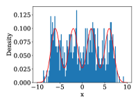
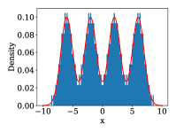
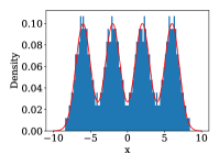
Figure 1: Histogram of the empirical distribution of $N=500$ particles at final time, simulated according to standard SVGD dynamics for $T=500$ time units. The first three are using a kernel of the form (4) for $p=2,1,\frac{1}{2}$, respectively. The last histogram employs a time-evolving kernel where the value of $p$ is evolved from $p_{0}=2$ to $p_{1}=\frac{1}{2}$. The red line denotes the target density.

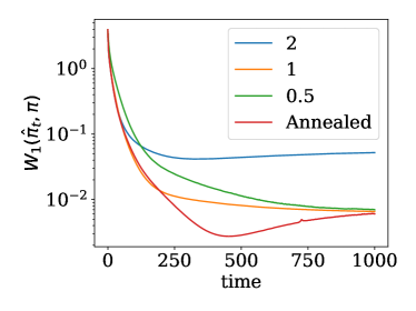
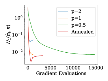
Figure 2: Time evolution of the Wasserstein-1 error between the target and empirical distributions arising from simulating SVGD from $0$ to $T$ and different values of $p$. In the left plot, the evolution is shown as a function of time. In the right plot, it is shown as a function of the number of gradient evaluations, reflecting the true computational cost.

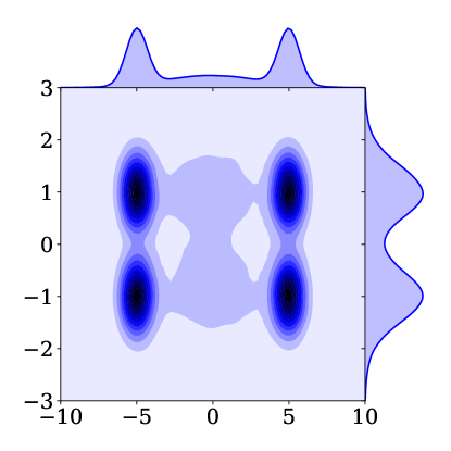
Figure 3: Target distribution for the two-dimensional Gaussian mixture model example.

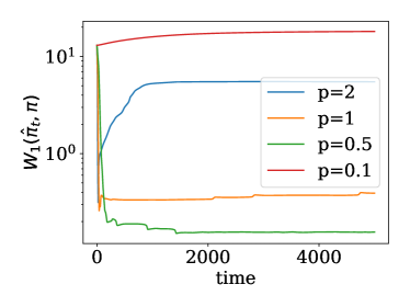
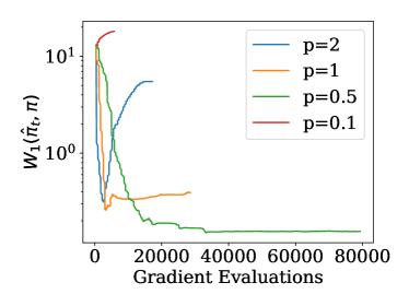
Figure 4: Time evolution of the Wasserstein-1 error between the target and empirical distributions arising from simulating SVGD from $0$ to $T$ and different values of $p$ for the two-dimensional mixture model example. In the left plot, the evolution is shown as a function of time. In the right plot, it is shown as a function of the number of gradient evaluations, reflecting the true computational cost.

9 Conclusions

In this paper we have analysed the geometric properties of SVGD related to its gradient flow interpretation. In particular, we have extended the framework put forward in Liu (2017), obtained the associated geodesic equations and used those results to derive functional inequalities connected to exponential convergence of SVGD dynamics close to equilibrium. We have leveraged the latter to develop principled guidelines for an appropriate choice of the kernel $k$ and verified those in numerical experiments. In particular, our theoretical considerations have led us to investigating singular kernels with adjusted tails.

There are various avenues for further research. First, it would be interesting to place the geometric calculations in the framework of metric spaces developed in Ambrosio et al. (2008), relaxing the regularity assumptions and placing in particular Proposition 20 on a more rigorous foundation. It will be of key importance to extend the results obtained in Section 6.1 to the multidimensional case. The numerical experiments have indicated that such an extension might be possible and yield further insights. Quantifying the speed of convergence for initial distributions far from equilibrium remains an open and challenging problem. As noted in Section 7, this might be possible (and first encouraging results are available) for polynomial kernels. Last but not least, we believe that understanding the properties of the finite-particle systems (1) and (9) (as opposed to the mean field limit (2)) will be important for further algorithmic advances. All of the preceding points are currently under investigation.

Acknowledgement. This research has been partially funded by Deutsche Forschungsgemeinschaft (DFG) through grant CRC 1114 ‘Scaling Cascades’ (project A02). NN would like to thank Alexander Mielke, Felix Otto and Sebastian Reich for stimulating discussions. AD was supported by the Lloyds Register Foundation Programme on Data Centric Engineering and by The Alan Turing Institute under the EPSRC grant [EP/N510129/1]. We would like to thank the anonymous referees whose very careful reading and thoughtful remarks have helped to substantially improve the paper.

Appendix A Analogies between Langevin dynamics and SVGD

In this appendix we will trace the similarities between overdamped Langevin dynamics and SVGD according to the gradient flow perspective. We note that a similar comparison has been made in Liu (2017, Section 3.5). Here our aim is to extend this discussion and place our results in this context.

A.1 Overdamped Langevin dynamics, the Fokker-Planck equation and optimal transport

To start with, let us consider the overdamped Langevin dynamics (Pavliotis, 2014, Section 4.5)

$$\mathrm{d}X_{t}=-\nabla V(X_{t})\,\mathrm{d}t+\sqrt{2}\,\mathrm{d}B_{t},\quad X_{0}=x_{0}.$$ (49)

It is well-known that under mild conditions on $V$ this SDE admits a unique strong solution $(X_{t})_{t\geq 0}$ that is ergodic with respect to $\pi\propto e^{-V}$, see, for instance, Roberts et al. (1996). This fact motivates using a suitable discretisation of (49) as a sampling scheme, laying the foundation for a number of (approximate) MCMC algorithms such as MALA and ULA (Robert and Casella, 2013, Section 6.5.2). The law of $X_{t}$, denoted by $\rho_{t}:=\operatorname{Law}(X_{t})$, solves the Fokker-Planck equation

$$\partial_{t}\rho =\nabla\cdot(\rho\nabla V+\nabla\rho)$$ (50a)

$$=\nabla\cdot\left(\rho(\nabla V+\nabla\log\rho)\right).$$ (50b)

The value of the reformulation (50b) becomes apparent when we notice that the Stein PDE (2) can be written in the form

$$\partial_{t}\rho=\nabla\cdot\left(\rho\mathcal{T}_{k,\rho}(\nabla V+\nabla\log\rho)\right),$$

see Lemma 11 and Corollary 13. In particular, the Fokker-Planck Onsager operator (Machlup and Onsager, 1953; Mielke et al., 2016; Öttinger, 2005)

$$\mathbb{K}_{\rho}^{FP}:\phi\mapsto-\nabla\cdot(\rho\nabla\phi),$$

should be compared to the Stein Onsager operator from Remark 12. As first observed in the seminal paper Jordan et al. (1998), the PDE (50) can be interpreted as the gradient flow of the $\mathrm{KL}$-divergence (21) with respect to the quadratic Wasserstein distance $\mathcal{W}_{2}$ using the Benamou-Brenier formula (Benamou and Brenier, 2000)

$$\mathcal{W}_{2}^{2}(\mu,\nu)=\inf_{(\rho,v)}\left\{\int_{0}^{1}\|v_{t}\|_{L^{2}(\rho_{t})}^{2}\,\mathrm{d}t:\quad\partial_{t}\rho+\nabla\cdot(\rho v)=0,\quad\rho_{0}=\mu,\,\rho_{1}=\nu\right\}.$$ (51)

As already noticed in Remark 18, the Stein distance $d_{k}$ essentially differs from $\mathcal{W}_{2}$ only by exchanging the $L^{2}(\rho)$-norm for the $\mathcal{H}_{k}^{d}$-norm. The infimum in (51) remains the same if optimisation is carried out over gradient fields $v=\nabla\phi$, see for instance Gigli (2012, Section 1.4). This is completely analogous to the optional constraint $v_{t}\in\overline{\mathcal{T}_{k,\rho_{t}}\nabla C_{c}^{\infty}(\mathbb{R}^{d})}^{\mathcal{H}_{k}^{d}}$ in Definition 15, see (24). The geodesics associated to the distances $d_{k}$ and $\mathcal{W}_{2}$ are described by the systems of equations (25) and (26). As already observed in Remark 21, the equations pertaining to the Stein geometry are coupled, reflecting the fact that SVGD is based on an evolution of interacting particles. In Otto and Villani (2000, Section 3), the Hessian of the $\mathrm{KL}$-divergence in the Wasserstein geometry was computed; this expression should naturally be compared to the Hessian in the Stein geometry, see Lemma 25. Notably, the Wasserstein-Hessian can be related to the Ricci-curvature of the underlying manifold, an observation that has sparked numerous developments within the intersection between geometry and probability (see for instance Villani (2009, Part III)). As of now we are not able to spot a similar connection in (32). We believe that a more intuitive (possibly geometric) understanding of (32) might lead to further algorithmic improvements of SVGD. Finally, the Wasserstein-Hessian has been leveraged in Otto (2001) for the analysis of certain functional inequalities central to the understanding of exponential convergence to equilibrium of the overdamped Langevin dynamics (49). We mention in particular the Poincaré inequality taking the same form as (39), but with $\mathcal{L}$ given by

$$\mathcal{L}\phi=-\sum_{i=1}^{d}e^{V}\partial_{i}\left(e^{-V}\partial_{i}\phi\right),$$ (52)

i.e. only differing by the operator $T_{k,\pi}$. The viewpoint of Otto and Villani (2000) led to a geometric understanding of the celebrated Bakry-Émery criterion (Otto and Villani, 2000, Theorem 2); we note that our condition (45) has a similar flavour (albeit in a simplified context). Despite all those similarities, we would like to stress that the Fokker-Planck equation (50) governs the law of (49) while the Stein PDE (2) arises as the mean-field limit for (1) and (9). This fact makes a direct theoretical comparison between the corresponding algorithms difficult, see Remark 31.

Appendix B Proofs for Section 3

Proof of Proposition 2    Let $\phi\in C_{c}^{\infty}([0,\infty)\times\mathbb{R}^{d})$ be a smooth test function with compact support and define $\Phi\in C_{c}^{\infty}([0,\infty)\times\mathbb{R}^{Nd})$ by $\Phi(t,x):=\frac{1}{N}\sum_{i=1}^{N}\phi(t,x_{i})$. Using the notation

$$b(x,\rho):=\int_{\mathbb{R}^{d}}\left[-k(x,y)\nabla V(y)+\nabla_{y}k(x,y)\right]\mathrm{d}\rho(y),$$

Itô’s formula implies

$$\mathrm{d}\Phi(t,\bar{X}_{t}) =\frac{1}{N}\sum_{i=1}^{N}\left(\partial_{t}\phi(t,X_{t}^{i})+\nabla\phi(t,X_{t}^{i})\cdot b(X_{t}^{i},\rho_{t}^{N})\right)\mathrm{d}t+\operatorname{Tr}\left(\mathcal{K}(\bar{X}_{t})\mathrm{Hess}\,\Phi(\bar{X}_{t})\right)\mathrm{d}t$$

$$\qquad+\frac{\sqrt{2}}{N}\sum_{i,j=1}^{N}\nabla\phi(X_{t}^{i})\cdot\sqrt{\mathcal{K}(\bar{X}_{t})}_{ij}\,\mathrm{d}W_{t}^{j}.$$

The Hessian $\mathrm{Hess}\,\Phi\in\mathbb{R}^{Nd\times Nd}$ consists of $N^{2}$ blocks of size $d\times d$ with

$$\left[\mathrm{Hess}\,\Phi(x)\right]_{ij}=\begin{cases}\frac{1}{N}\mathrm{Hess}\,\phi(x_{i})&\mbox{if }i=j\\ 0&\mbox{otherwise}\end{cases},\quad(i,j)\in\{1,\ldots,N\}^{2},$$

so that it is a block diagonal matrix, with each diagonal block containing the Hessian of $\phi$.

A simple calculation yields that

$$\operatorname{Tr}(\mathcal{K}(x)\mathrm{Hess}\,\Phi(x))=\frac{1}{N^{2}}\sum_{i=1}^{N}k(x_{i},x_{i})\operatorname{Tr}(\mathrm{Hess}\,\phi(x_{i}))=\frac{1}{N^{2}}\sum_{i=1}^{N}k(x_{i},x_{i})\Delta\phi(x_{i}),$$

so that

$$\operatorname{Tr}\left(\mathcal{K}(\bar{X}_{t})\mathrm{Hess}\,\Phi(\bar{X}_{t})\right)=\frac{1}{N}\int_{\mathbb{R}^{d}}k(x,x)\Delta\phi(x)\,\mathrm{d}\rho_{t}^{N}(x).$$

It follows that

$$\langle\phi(t,\cdot),\rho_{t}^{N}\rangle-\langle\phi(0,\cdot),\rho_{0}^{N}\rangle =\int_{0}^{t}\langle\partial_{s}\phi(s,\cdot),\rho_{s}^{N}\rangle\,\mathrm{d}s+\int_{0}^{t}\langle\nabla\phi(s,\cdot)\cdot b(\cdot,\rho_{s}^{N}),\rho_{s}^{N}\rangle\,\mathrm{d}s$$

$$\qquad+\frac{1}{N}\int_{0}^{t}\langle k(\cdot,\cdot)\Delta\phi(\cdot),\rho_{s}^{N}\rangle\,\mathrm{d}s+\mathcal{N}_{t},$$

where the brackets denote the duality pairing between test functions and measures. The term $\mathcal{N}_{t}$ represents a local martingale with quadratic variation

$$[\mathcal{N}_{\cdot},\mathcal{N}_{\cdot}]_{t} =\frac{2}{N^{2}}\int_{0}^{t}\sum_{i,j=1}^{N}\nabla\phi(X_{s}^{i})\cdot\mathcal{K}(\bar{X}_{s})_{ij}\nabla\phi(X_{s}^{j})\,\mathrm{d}s$$

$$=\frac{2}{N^{3}}\int_{0}^{t}\sum_{i,j=1}^{N}\nabla\phi(X_{s}^{i})\cdot\nabla\phi(X_{s}^{j})\,k(X_{s}^{i},X_{s}^{j})\,\mathrm{d}s$$

$$=\frac{2}{N}\int_{0}^{t}\int_{\mathbb{R}^{d}}\int_{\mathbb{R}^{d}}\nabla\phi(y)\cdot\nabla\phi(z)k(y,z)\,\mathrm{d}\rho_{s}^{N}(y)\,\mathrm{d}\rho_{s}^{N}(z)\,\mathrm{d}s.$$

In particular, assuming that the family $\{\rho_{\cdot}^{N}\>:\>N\in\mathbb{N}\}$ possesses a limit point in $\mathcal{P}(C[0,T])$, it follows that $[\mathcal{N}_{\cdot},\mathcal{N}_{\cdot}]_{t}\sim O(N^{-1})$ as $N\rightarrow\infty.$ Let $\rho_{\cdot}$ be a limit point of the family $\{\rho_{\cdot}^{N}\>:\>N\in\mathbb{N}\}$, then formally as $N\rightarrow\infty$ we obtain the following relationship for the limiting distribution:

$$\langle\phi(t,\cdot),\rho_{t}\rangle-\langle\phi(0,\cdot),\rho_{0}\rangle=\int_{0}^{t}\langle\partial_{s}\phi(s,\cdot),\rho_{s}\rangle\,\mathrm{d}s+\int_{0}^{t}\langle\nabla\phi(s,\cdot)\cdot b(\cdot,\rho_{s}),\rho_{s}\rangle\,\mathrm{d}s,$$

so that the limit $\rho_{t}=\lim_{N\rightarrow\infty}\rho_{t}^{N}$ satisfies the nonlinear transport equation

$$\partial_{t}\rho_{t}(t,x)=-\nabla\cdot(b(x,\rho_{t})\rho_{t}),$$

as required.  

Proof of Proposition 3   For a textbook account of similar proof strategies we refer to Khasminskii (2011), see also the proof of Theorem 3.1 in Meyn and Tweedie (1993). Let us define the set

$$D:=(\mathbb{R}^{d})^{N}\setminus\bigcup_{i\neq j}\left\{(x_{1},\ldots,x_{n})\in(\mathbb{R}^{d})^{N}:\quad x_{i}=x_{j}\right\}$$

and the Lyapunov function

$$F(\bar{x})=\sum_{\begin{subarray}{c}l,m=1\\ l\neq m\end{subarray}}^{N}F_{lm}(x_{l},x_{m}),\quad\bar{x}=(x_{1}\ldots,x_{N})\in D,$$ (53)

with

$$F_{lm}(x_{l},x_{m})=-\frac{1}{2}\chi(|x_{l}-x_{m}|^{2})\log|x_{l}-x_{m}|^{2}.$$

Here $\chi\in C_{c}^{\infty}(\mathbb{R})$ is assumed to be a fixed nonnegative cutoff function with $\chi\equiv 1$ on $[0,1]$. We now argue that there exist constants $C_{1},C_{2}\in\mathbb{R}$ such that

$$(\bar{L}F)(\bar{x})\leq C_{1}\sum_{i=1}^{N}|\nabla V(x_{i})|+C_{2},\quad\bar{x}=(x_{1},\ldots x_{N})\in D,$$ (54)

where $\bar{L}$ is the infinitesimal generator of (9),

$$\bar{L}\phi=-\nabla\bar{V}\cdot\mathcal{K}\nabla\phi+(\nabla\cdot\mathcal{K})\cdot\nabla\phi+\mathcal{K}:\nabla\nabla\phi,\quad\phi\in\mathcal{D}(\bar{L}).$$ (55)

For $l\neq m$, we see that

$$\left(-\nabla\bar{V}\cdot\mathcal{K}\nabla F_{lm}\right)(\bar{x})= -\chi\left(|x_{l}-x_{m}|^{2}\right)\sum_{i=1}^{N}\nabla V(x_{i})\cdot\frac{x_{l}-x_{m}}{(x_{l}-x_{m})^{2}}\left(h(x_{i}-x_{m})-h(x_{i}-x_{l})\right)$$ (56a)

$$+\frac{1}{2}\log|x_{l}-x_{m}|^{2}\sum_{i,j=1}^{N}\nabla V(x_{i})\cdot h(x_{i}-x_{j})\nabla_{x_{j}}\chi\left(|x_{l}-x_{m}|^{2}\right)$$ (56b)

$$\leq\tilde{C}_{1}\sum_{i=1}^{N}|\nabla V(x_{i})|+\tilde{C}_{2},$$ (56c)

where here and in what follows $\tilde{C}_{1}$ and $\tilde{C}_{2}$ denote generic constants, the value of which can change from line to line. The estimate (56c) follows from the fact that (56b) is bounded (with compact support) by the construction of $\chi$, and by using Lipschitz continuity of $h$ in (56a). Similarly, we have that

$$\left((\nabla\cdot\mathcal{K})\cdot\nabla F_{lm}\right)(\bar{x}) =\sum_{i,j=1}^{N}\nabla_{x_{i}}h(x_{i}-x_{j})\cdot\nabla_{x_{j}}F_{lm}(x_{l},x_{m})$$ (57a)

$$=\chi(|x_{l}-x_{m}|^{2})\sum_{i=1}^{N}\left(\nabla_{x_{i}}(h(x_{i}-x_{m})-h(x_{i}-x_{l})\right)\cdot\frac{x_{l}-x_{m}}{(x_{l}-x_{m})^{2}}$$ (57b)

$$-\log|x_{l}-x_{m}|^{2}\chi^{\prime}(|x_{l}-x_{m}|^{2})\sum_{i=1}^{N}\nabla_{x_{i}}\left(h(x_{i}-x_{l})-h(x_{i}-x_{m})\right)\cdot(x_{l}-x_{m})$$ (57c)

is bounded due to the one-sided Lipschitz bound (13). Lastly,

$$\left(\mathcal{K}:\nabla\nabla F_{lm}\right)(\bar{x}) =\sum_{i,j=1}^{N}h(x_{i}-x_{j})\nabla_{x_{i}}\cdot\nabla_{x_{j}}F_{lm}=-\sum_{i=1}^{N}\left(h(x_{i}-x_{l})-h(x_{i}-x_{m})\right)\nabla_{x_{i}}\cdot$$ (58a)

$$\cdot\left(\log|x_{l}-x_{m}|^{2}\chi^{\prime}\left(|x_{l}-x_{m}|^{2}\right)(x_{l}-x_{m})+\chi\left(|x_{l}-x_{m}|^{2}\right)\frac{x_{l}-x_{m}}{(x_{l}-x_{m})^{2}}\right)$$ (58b)

$$\leq\tilde{C}-2\chi\left(|x_{l}-x_{m}|^{2}\right)\frac{d-2}{(x_{l}-x_{m})^{2}}\left(h(0)-h(x_{m}-x_{l})\right),$$ (58c)

where we have again subsumed terms that are bounded by the construction of $\chi$ in the constant $\tilde{C}$. Note that the second term in (58c) (including the minus sign) is nonpositive since $h$ is a positive definite function (see, for instance, Fasshauer (2007, Theorem 3.1(4))). Collecting (56), (57) and (58), we indeed arrive at the Lyapunov bound (54).

Now note that $F$ is bounded from below, and so we can choose a constant $c$ such that $\tilde{F}:=F+c$ is nonnegative. By the assumption that the initial condition is distinct, there exists $q_{0}\in\mathbb{N}$ such that $\tilde{F}(\bar{X}_{0})<q_{0}$. For $q>q_{0}$ let us define the stopping times

$$\tau_{q}=\inf\{t\geq 0:\quad\tilde{F}(\bar{X}_{t})=q\}.$$

By Dynkin’s formula in combination with the bound (54) and Assumption 4, we see that

$$\mathbb{E}[\tilde{F}(\bar{X}_{\tau_{q}\wedge t})]<C_{t},$$ (59)

for all $q>q_{0}$ and a constant $C_{t}$ that depends on $t$, but not on $q$. On the other hand,

$$\mathbb{E}[\tilde{F}(\bar{X}_{\tau_{q}\wedge t})]=\mathbb{E}[\tilde{F}(\bar{X_{t}})\mathbf{1}_{\{t<\tau_{q}\}}]+q\mathbb{P}[t\geq\tau_{q}]\geq q\mathbb{P}[t\geq\tau_{q}],$$ (60)

where we have used the fact that $\tilde{F}$ is nonnegative. This, together with (59), immediately implies $\mathbb{P}[t\geq\xi]=0$ for all $t\geq 0$, where $\xi:=\lim_{q\rightarrow\infty}\tau_{q}$. Monotone convergence then shows that $\mathbb{P}[\xi=\infty]=1$.

In other words, we have shown that $\bar{X}_{t}\in D$ almost surely, for all $t\geq 0$. Since $\mathcal{K}$ is strictly positive definite on $D$, there is an invariant measure with strictly positive Lebesgue density (see (11)) and $D$ is path-connected (Bolley et al., 2018, Lemma 3.1), it follows that the process is irreducible and hence ergodic with unique invariant measure (11), see Kliemann (1987).  

Appendix C Proofs for Section 4

Let us begin with the following auxiliary lemma:

Lemma 47

Let $\rho\in\mathcal{P}_{k}(\mathbb{R}^{d})$. Then $\overline{\mathcal{T}_{k,\rho}\nabla C_{c}^{\infty}(\mathbb{R}^{d})}^{\mathcal{H}_{k}^{d}}$ is the orthogonal complement of $L^{2}_{\mathrm{div}}(\rho)\cap\mathcal{H}_{k}^{d}$ in $\mathcal{H}^{d}_{k}$, where $L^{2}_{\mathrm{div}}(\rho)$ is the space of weighted divergence-free vector fields, i.e.

$$L^{2}_{\mathrm{div}}(\rho)=\left\{v\in(L^{2}(\rho))^{d}:\langle v,\nabla\phi\rangle_{L^{2}(\rho)}=0\quad\text{for all }\phi\in C_{c}^{\infty}(\mathbb{R}^{d})\right\}.$$ (61)

Moreover, $L^{2}_{\mathrm{div}}(\rho)\cap\mathcal{H}_{k}^{d}$ is closed in $\mathcal{H}_{k}^{d}$.

Proof of Proposition 6 We begin by showing that $\overline{\mathcal{T}_{k,\rho}\nabla C_{c}^{\infty}(\mathbb{R}^{d})}^{\mathcal{H}_{k}^{d}}$ is the orthogonal complement of $L^{2}_{\mathrm{div}}(\rho)\cap\mathcal{H}_{k}^{d}$ in $\mathcal{H}^{d}_{k}$. Indeed, using the relation $(U^{\perp})^{\perp}=\overline{U}$ valid for arbitrary linear subspaces of Hilbert spaces, it is enough to show that

$$\left(\mathcal{T}_{k,\rho}\nabla C_{c}^{\infty}(\mathbb{R}^{d})\right)^{\perp_{\mathcal{H}_{k}^{d}}}=L^{2}_{\mathrm{div}}(\rho)\cap\mathcal{H}_{k}^{d}.$$ (62)

By Steinwart and Christmann (2008, Theorem 4.26), we have that $\mathcal{T}_{k,\rho}$ is the adjoint of the inclusion $\mathcal{H}_{k}^{d}\hookrightarrow(L^{2}(\rho))^{d}$, implying

$$\langle v,\nabla\phi\rangle_{L^{2}(\rho)}=\langle v,\mathcal{T}_{k,\rho}\nabla\phi\rangle_{\mathcal{H}^{d}_{k}},$$ (63)

for all $v\in\mathcal{H}_{k}^{d}$ and $\phi\in C_{c}^{\infty}(\mathbb{R}^{d})$. This proves (62) and thus the orthogonality statement follows. We next show that $L^{2}_{\mathrm{div}}(\rho)\cap\mathcal{H}_{k}^{d}$ is closed in $\mathcal{H}_{k}^{d}$. For that, let $(v_{n})\subset L^{2}_{\mathrm{div}}(\rho)\cap\mathcal{H}_{k}^{d}$ with $v_{n}\rightarrow v$ in $\mathcal{H}_{k}^{d}$. Using (63) we see that $v\in L^{2}_{\mathrm{div}}(\rho)$, implying that $L^{2}_{\mathrm{div}}(\rho)\cap\mathcal{H}_{k}^{d}$ is closed. The statement of Proposition 6 now follows from Theorem II.3 in Reed et al. (1972).  
We now turn to the proof of Lemma 9.

Proof of Lemma 9   We only prove the second claim, as it immediately implies the first one. Assume that for $\xi\in T_{\rho}M$ there exist $v,w\in\overline{\mathcal{T}_{k,\rho}\nabla C_{c}^{\infty}(\mathbb{R}^{d})}^{\mathcal{H}_{k}^{d}}$ such that

$$\xi+\nabla\cdot(\rho v)=\xi+\nabla\cdot(\rho w)=0$$

in the sense of distributions. It follows immediately that

$$\int_{\mathbb{R}^{d}}\nabla\phi\cdot(v-w)\,\mathrm{d}\rho=0,$$

for all $\phi\in C_{c}^{\infty}(\mathbb{R}^{d})$, i.e. $v-w\in L^{2}_{\mathrm{div}}(\rho)$. Since $\overline{\mathcal{T}_{k,\rho}\nabla C_{c}^{\infty}(\mathbb{R}^{d})}^{\mathcal{H}_{k}^{d}}\cap L^{2}_{\mathrm{div}(\rho)}=\{0\}$ by Lemma 47 and $v-w\in\overline{\mathcal{T}_{k,\rho}\nabla C_{c}^{\infty}(\mathbb{R}^{d})}^{\mathcal{H}_{k}^{d}}$, we conclude that $v=w$. Consequently, the map $v\mapsto\nabla(\rho v)$ is a bijection. The fact that it is also an isometry follows directly from the definition of $g_{\rho}$.  

Proof of Lemma 11   By definition, the Riemannian gradient $\mathrm{grad}_{\rho}\mathcal{F}\in T_{\rho}M$ is determined by the requirement that

$$g_{\rho}\left(\mathrm{grad}_{\rho}\mathcal{F},\partial_{t}\mu_{t}\Big{|}_{t=0}\right)=\frac{\mathrm{d}}{\mathrm{d}t}\mathcal{F}(\mu_{t})\Big{|}_{t=0},$$ (64)

for all sufficiently regular curves $(\mu_{t})_{t\in(-\varepsilon,\varepsilon)}\subset M$ with $\mu_{0}=\rho$ and $\partial_{t}\mu_{t}\Big{|}_{t=0}\in T_{\rho}M$. Given such a curve and corresponding vector fields $(w_{t})_{t\in(-\varepsilon,\varepsilon)}$ satisfying $\partial_{t}\mu+\nabla\cdot(\mu w)=0$ in the sense of distributions, we compute the right-hand side of (64),

$$\frac{\mathrm{d}}{\mathrm{d}t}\mathcal{F}(\mu_{t})\Big{|}_{t=0}=\int_{\mathbb{R}^{d}}\frac{\delta\mathcal{F}}{\delta\mu}(\mu_{t})\,\partial_{t}\mu_{t}\,\mathrm{d}x\Big{|}_{t=0}=\int_{\mathbb{R}^{d}}\nabla\frac{\delta\mathcal{F}}{\delta\rho}(\rho)\cdot w_{0}\,\mathrm{d}\rho.$$

From the definition of $T_{\rho}M$, we have that $\partial_{t}\mu_{t}\Big{|}_{t=0}\in T_{\rho}M$ implies $w_{0}\in\mathcal{H}_{k}^{d}$. Therefore, using Steinwart and Christmann (2008, Theorem 4.26), we can write

$$\int_{\mathbb{R}^{d}}\nabla\frac{\delta\mathcal{F}}{\delta\rho}(\rho)\cdot w_{0}\,\mathrm{d}\rho=\left\langle\mathcal{T}_{k,\rho}\nabla\frac{\delta\mathcal{F}}{\delta\rho}(\rho),w_{0}\right\rangle_{\mathcal{H}_{k}^{d}}.$$ (65)

From the definition of $g_{\rho}$, the left-hand side of (64) can be expressed as

$$g_{\rho}\left(\mathrm{grad}_{\rho}\mathcal{F},\partial_{t}\mu_{t}\Big{|}_{t=0}\right)=\langle v,w_{0}\rangle_{\mathcal{H}_{k}^{d}},$$ (66)

where $\mathrm{grad}_{\rho}\mathcal{F}+\nabla\cdot(\rho v)=0$, $v\in\overline{\mathcal{T}_{k,\rho}\nabla C_{c}^{\infty}(\mathbb{R}^{d})}$. Now imposing equality of (65) and (66) for all $w_{0}\in\overline{\mathcal{T}_{k,\rho}\nabla C_{c}^{\infty}(\mathbb{R}^{d})}$ leads to the desired result.  

Proof of Lemma 17

1.) We recall that metrics by definition satisfy the axioms

$$d_{k}(\mu_{1},\mu_{2})\geq 0,\quad\quad$$ (nonnegativity) (67a)

$$d_{k}(\mu_{1},\mu_{2})=d_{k}(\mu_{2},\mu_{1}),\quad\quad$$ (symmetry) (67b)

$$d_{k}(\mu_{1},\mu_{2})=0\quad\iff\quad\mu_{1}=\mu_{2},\quad\quad$$ (nondegeneracy) (67c)

$$d_{k}(\mu_{1},\mu_{2})+d_{k}(\mu_{2},\mu_{3})\leq d_{k}(\mu_{1},\mu_{3}),\quad\quad$$ (triangle inequality) (67d)

for $\mu_{1},\mu_{2},\mu_{3}\in M$. The properties (67a) and (67c) follow directly from the definition of $d_{k}$. For (67b) note that $(\rho_{t},v_{t})_{t\in[0,1]}\in\mathcal{A}(\mu,\nu)$ if and only if $(\rho_{1-t},-v_{1-t})_{t\in[0,1]}\in\mathcal{A}(\nu,\mu)$ as well as $v\in\overline{\mathcal{T}_{k,\rho}\nabla C_{c}^{\infty}(\mathbb{R}^{d})}$ if and only if $-v\in\overline{\mathcal{T}_{k,\rho}\nabla C_{c}^{\infty}(\mathbb{R}^{d})}$. The triangle inequality (67d) follows from considering concatenated paths from $\mu_{1}$ to $\mu_{3}$ via $\mu_{2}$.

2.) From Steinwart and Christmann (2008, Theorem 4.26) we have that

$$\|v\|_{L^{2}(\rho)}\leq\int_{\mathbb{R}^{d}}k(x,x)\,\mathrm{d}\rho(x)\,\|v\|_{\mathcal{H}_{k}^{d}},\quad v\in\mathcal{H}_{k}^{d}.$$

The claim now follows directly from the Benamou-Brenier formula for the quadratic Wasserstein distance, see Benamou and Brenier (2000), together with Lemma 17.3.

3.) For fixed $\mu,\nu\in M$, consider a connecting curve $(\rho,v)\in\mathcal{A}(\mu,\nu)$. According to Lemma 47 we have the $\mathcal{H}_{k}^{d}$-orthogonal decompositions

$$\mathcal{H}_{k}^{d}=\overline{\mathcal{T}_{k,\rho_{t}}\nabla C_{c}^{\infty}(\mathbb{R}^{d})}^{\mathcal{H}_{k}^{d}}\oplus\left(L^{2}_{\mathrm{div}}(\rho_{t})\cap\mathcal{H}_{k}^{d}\right),\quad t\in[0,1],$$ (68)

i.e. we can write

$$v_{t}=u_{t}+w_{t},\quad u_{t}\in\overline{\mathcal{T}_{k,\rho_{t}}\nabla C_{c}^{\infty}(\mathbb{R}^{d})}^{\mathcal{H}_{k}^{d}},\quad w_{t}\in L^{2}_{\mathrm{div}}(\rho_{t})\cap\mathcal{H}_{k}^{d},$$

with $(u_{t})_{t\in[0,1]}$ and $(w_{t})_{t\in[0,1]}$ being uniquely determined. Since $w_{t}\in L^{2}_{\mathrm{div}}(\rho_{t})$ for all $t\in[0,1]$, we have that $v$ satisfies the continuity equation (23) if and only if $u$ does. By $\mathcal{H}_{k}^{d}$-orthogonality in (68), we moreover have

$$\|v_{t}\|^{2}_{\mathcal{H}_{k}^{d}}=\|u_{t}\|_{\mathcal{H}_{k}^{d}}^{2}+\|w_{t}\|_{\mathcal{H}_{k}^{d}}^{2},\quad t\in[0,1].$$ (69)

Because (69) is optimised for $w_{t}=0$ while keeping the continuity equation unchanged, it is clear that the objective in (24) enforces $w_{t}=0$, or, equivalently, $v_{t}\in\overline{\mathcal{T}_{k,\rho_{t}}\nabla C_{c}^{\infty}(\mathbb{R}^{d})}^{\mathcal{H}_{k}^{d}}$, for all $t\in[0,1]$.  

Appendix D Proofs for Section 5

Proof of Proposition 20   The arguments are formal and proceed along the lines of Otto and Villani (2000, Section 3). In (22) let us substitute $v_{t}=\mathcal{T}_{k,\rho_{t}}\nabla\Phi_{t}$ with $\Phi_{t}\in C_{c}^{\infty}(\mathbb{R}^{d})$, $t\in[0,1]$, to obtain

$$d_{k}^{2}(\mu,\nu)=\inf_{(\rho,\Phi)}\left\{\int_{0}^{1}\|\mathcal{T}_{k,\rho_{t}}\nabla\Phi_{t}\|_{\mathcal{H}_{k}^{d}}^{2}\,\mathrm{d}t:\quad\partial_{t}\rho+\nabla\cdot(\rho\mathcal{T}_{k,\rho}\nabla\Phi)=0,\quad\rho_{0}=\mu,\quad\rho_{1}=\nu\right\},$$ (70)

where the continuity equation is as usual interpreted in a weak sense, i.e. the pair $(\rho,\Phi)$ satisfies the constraints in (70) if and only if

$$-\int_{0}^{1}\int_{\mathbb{R}^{d}}\partial_{t}\Psi\,\mathrm{d}\rho\,\mathrm{d}t-\int_{0}^{1}\langle\nabla\Psi,\mathcal{T}_{k,\rho}\nabla\Phi\rangle_{L^{2}(\rho)}\,\mathrm{d}t+\int_{\mathbb{R}^{d}}\Psi_{1}\,\mathrm{d}\nu-\int_{\mathbb{R}^{d}}\Psi_{0}\,\mathrm{d}\mu=0,$$ (71)

for all test functions $\Psi\in C_{c}^{\infty}([0,1]\times\mathbb{R}^{d})$. Let us now define the following functional on pairs $(\rho,\Phi)$,

$$\mathcal{E}(\rho,\Phi):=\sup_{\Psi}\left\{-\int_{0}^{1}\int_{\mathbb{R}^{d}}\partial_{t}\Psi\,\mathrm{d}\rho\,\mathrm{d}t-\int_{0}^{1}\langle\nabla\Psi,\mathcal{T}_{k,\rho}\nabla\Phi\rangle_{L^{2}(\rho)}\,\mathrm{d}t+\int_{\mathbb{R}^{d}}\Psi_{1}\,\mathrm{d}\nu-\int_{\mathbb{R}^{d}}\Psi_{0}\,\mathrm{d}\mu\right\},$$

where the supremum is taken over all $\Psi\in C_{c}^{\infty}([0,1]\times\mathbb{R}^{d})$. Since the expression inside the supremum is linear in $\Psi$, it follows that $\mathcal{E}$ characterises weak solutions in the sense of (71) in the following way,

$$\mathcal{E}(\rho,\Phi)=\begin{cases}0&\text{if }(\rho,\Phi)\,\text{solves \eqref{eq:weak cont},}\\ +\infty&\text{otherwise.}\end{cases}$$ (72a)

We can therefore write

$$\frac{1}{2}d_{k}^{2}(\mu,\nu) =\inf_{(\rho,\Phi)}\sup_{\Psi}\left\{\frac{1}{2}\int_{0}^{1}\|\mathcal{T}_{k,\rho_{t}}\nabla\Phi_{t}\|_{\mathcal{H}_{k}^{d}}^{2}\,\mathrm{d}t+\mathcal{E}(\rho,\Phi)\right\}$$ (73a)

$$=\inf_{(\rho,\Phi)}\sup_{\Psi}\Bigg{\{}\frac{1}{2}\int_{0}^{1}\|\mathcal{T}_{k,\rho_{t}}\nabla\Phi_{t}\|_{\mathcal{H}_{k}^{d}}^{2}\,\mathrm{d}t$$ (73b)

$$-\int_{0}^{1}\int_{\mathbb{R}^{d}}\partial_{t}\Psi\,\mathrm{d}\rho\,\mathrm{d}t-\int_{0}^{1}\int_{0}^{1}\langle\nabla\Psi,\mathcal{T}_{k,\rho}\nabla\Phi\rangle_{L^{2}(\rho)}\,\mathrm{d}t+\int_{\mathbb{R}^{d}}\Psi_{1}\,\mathrm{d}\nu-\int_{\mathbb{R}^{d}}\Psi_{0}\,\mathrm{d}\mu\Bigg{\}}.$$ (73c)

The term in brackets in (73b)-(73c) is convex in $\Phi$ and concave (in fact, linear) in $\Psi$. Hence, it is justified to exchange infimum and supremum (see Rockafellar (1970),Villani (2003a, Section 1.1.6)) to obtain

$$\frac{1}{2}d_{k}^{2}(\mu,\nu) =\inf_{\rho}\sup_{\Psi}\Bigg{\{}-\int_{0}^{1}\int_{\mathbb{R}^{d}}\partial_{t}\Psi\,\mathrm{d}\rho\,\mathrm{d}t+\int_{\mathbb{R}^{d}}\Psi_{1}\,\mathrm{d}\nu-\int_{\mathbb{R}^{d}}\Psi_{0}\,\mathrm{d}\mu$$ (74a)

$$+\inf_{\Phi}\left\{\frac{1}{2}\int_{0}^{1}\left(\|\mathcal{T}_{k,\rho_{t}}\nabla\Phi_{t}\|_{\mathcal{H}_{k}^{d}}^{2}\,\mathrm{d}t-\langle\nabla\Psi,\mathcal{T}_{k,\rho_{t}}\nabla\Phi\rangle_{L^{2}(\rho_{t})}\right)\mathrm{d}t\right\}\Bigg{\}}.$$ (74b)

Using the fact that $\mathcal{T}_{k,\rho}$ is self-adjoint in $L^{2}(\rho)$ and that $\mathcal{T}_{k,\rho}^{1/2}:L^{2}(\rho)\rightarrow\mathcal{H}_{k}$ is an isometry (Steinwart and Christmann, 2008, Section 4.3), we see that

$$\langle\nabla\Psi,\mathcal{T}_{k,\rho_{t}}\nabla\Phi\rangle_{L^{2}(\rho_{t})}=\langle\mathcal{T}_{k,\rho_{t}}^{1/2}\nabla\Psi,\mathcal{T}_{k,\rho_{t}}^{1/2}\nabla\Phi\rangle_{L^{2}(\rho_{t})}=\langle\mathcal{T}_{k,\rho_{t}}\nabla\Psi,\mathcal{T}_{k,\rho_{t}}\nabla\Phi\rangle_{\mathcal{H}_{k}^{d}}.$$ (75)

Substituting into (74b), it follows that

$$\operatorname*{arg\,inf}_{\Phi}\left\{\frac{1}{2}\int_{0}^{1}\left(\|\mathcal{T}_{k,\rho_{t}}\nabla\Phi_{t}\|_{\mathcal{H}_{k}^{d}}^{2}\,\mathrm{d}t-\langle\nabla\Psi,\mathcal{T}_{k,\rho_{t}}\nabla\Phi\rangle_{L^{2}(\rho_{t})}\mathrm{d}t\right)\right\}=\Psi,$$

up to an additive constant, i.e.

$$\inf_{\Phi}\left\{\frac{1}{2}\int_{0}^{1}\left(\|\mathcal{T}_{k,\rho_{t}}\nabla\Phi_{t}\|_{\mathcal{H}_{k}^{d}}^{2}\,\mathrm{d}t-\langle\nabla\Psi,\mathcal{T}_{k,\rho_{t}}\nabla\Phi\rangle_{L^{2}(\rho_{t})}\right)\mathrm{d}t\right\}=-\frac{1}{2}\int_{0}^{1}\|\mathcal{T}_{k,\rho_{t}}\nabla\Psi_{t}\|_{\mathcal{H}_{k}^{d}}^{2}\mathrm{d}t.$$

Using (75), we obtain the expression

$$\frac{1}{2}\|\mathcal{T}_{k,\rho}\nabla\Psi\|_{\mathcal{H}_{k}^{d}}^{2}=\frac{1}{2}\int_{\mathbb{R}^{d}}\int_{\mathbb{R}^{d}}\nabla\Psi(x)k(x,y)\nabla\Psi(y)\,\mathrm{d}\rho(x)\mathrm{d}\rho(y).$$

Therefore, formally, we can compute the functional derivatives (see (19)),

$$\frac{\delta}{\delta\rho}\left(\frac{1}{2}\|\mathcal{T}_{k,\rho}\nabla\Psi\|_{\mathcal{H}_{k}^{d}}^{2}\right)(x) =\int_{\mathbb{R}^{d}}k(x,y)\,\nabla\Psi(x)\cdot\nabla\Psi(y)\,\mathrm{d}\rho(y)=\nabla\Psi(x)\cdot(\mathcal{T}_{k,\rho}\nabla\Psi)(x),$$ (76a)

$$\frac{\delta}{\delta\Psi}\left(\frac{1}{2}\|\mathcal{T}_{k,\rho}\nabla\Psi\|_{\mathcal{H}_{k}^{d}}^{2}\right)(x) =\nabla_{x}\cdot\left(\rho(x)\int_{\mathbb{R}^{d}}k(x,y)\nabla\Psi(y)\,\mathrm{d}\rho(y)\right)=\nabla\cdot\left(\rho\mathcal{T}_{k,\rho}\nabla\Psi\right)(x).$$ (76b)

The formal optimality conditions for (74) are therefore given by the system (25).  

Proof of Lemma 30   Dealing first with (83b)-(83c) and noting $\nabla\Psi=a$, we observe that

$$\sum_{i,j=1}^{d}\int_{\mathbb{R}^{d}}\int_{\mathbb{R}^{d}}\int_{\mathbb{R}^{d}}a_{i}a_{j}{\left(\partial_{x_{i}}\partial_{x_{j}}k(x,y)\right)\left(k(y,z)-k(x,z)\right)}\,\mathrm{d}\rho(x)\mathrm{d}\rho(y)\mathrm{d}\rho(z)=0,$$

since $\partial_{x_{i}}\partial_{x_{j}}k(x,y)=\partial_{x_{i}}\partial_{x_{j}}k(y,x)$ and $\left(k(y,z)-k(x,z)\right)=-\left(k(x,z)-k(y,z)\right)$. We hence obtain

$$\mathrm{Hess}_{\rho}(\Psi,\Psi) =\sum_{i,l=1}^{d}a_{i}^{2}\int_{\mathbb{R}^{d}}\int_{\mathbb{R}^{d}}\int_{\mathbb{R}^{d}}\partial_{x_{l}}k(x,y)\partial_{y_{l}}k(y,z)\,\mathrm{d}\rho(x)\mathrm{d}\rho(y)\mathrm{d}\rho(z)$$ (77a)

$$=-\sum_{i,l=1}^{d}a_{i}^{2}\int_{\mathbb{R}^{d}}\left(\int_{\mathbb{R}^{d}}k(x,y)\partial_{x_{l}}\rho(x)\,\mathrm{d}x\right)^{2}\mathrm{d}\rho(y)<0.$$ (77b)

The inequality is strict since $k$ is assumed to be integrally strictly positive definite, and the density $\rho$ cannot be constant.  

Appendix E Proof of Lemma 25

The proof proceeds by direct calculation, using the geodesic equations (25). For convenience, let us introduce the notation

$$w=\mathcal{T}_{k,\rho}\nabla\Psi.$$ (78)

The following lemma will come in handy.

Lemma 48

Let $\rho$ and $\Psi$ be smooth solutions to (25). Then

$$\partial_{t}w_{i}=-\sum_{j=1}^{d}\int_{\mathbb{R}^{d}}k(\cdot,y)\partial_{j}\Psi(y)\partial_{i}w_{j}(y)\,\mathrm{d}\rho(y)-\sum_{j=1}^{d}\int_{\mathbb{R}^{d}}k(\cdot,y)\partial_{j}\left(\partial_{i}\Psi(y)w_{j}(y)\rho(y)\right)\mathrm{d}y,$$ (79)

for $i=1,\ldots,d$.

Proof  By direct calculation, we obtain

$$\partial_{t}w_{i} =\int_{\mathbb{R}^{d}}k(\cdot,y)\left[\partial_{i}(\partial_{t}\Psi)\right](y)\,\mathrm{d}\rho(y)+\int_{\mathbb{R}^{d}}k(\cdot,y)\left[\partial_{i}\Psi\partial_{t}\rho\right](y)\,\mathrm{d}y$$ (80a)

$$=-\sum_{j=1}^{d}\int_{\mathbb{R}^{d}}k(\cdot,y)\left[\partial_{i}((\partial_{j}\Psi)w_{j})\right](y)\,\mathrm{d}\rho(y)-\sum_{j=1}^{d}\int_{\mathbb{R}^{d}}k(\cdot,y)\left[\partial_{i}\Psi(y)\partial_{j}(\rho w_{j})\right](y)\,\mathrm{d}y$$ (80b)

$$=-\sum_{j=1}^{d}\int_{\mathbb{R}^{d}}k(\cdot,y)\partial_{j}\Psi(y)\partial_{i}w_{j}(y)\,\mathrm{d}\rho(y)-\sum_{j=1}^{d}\int_{\mathbb{R}^{d}}k(\cdot,y)\partial_{j}\left(\partial_{i}\Psi(y)w_{j}(y)\rho(y)\right)\mathrm{d}y.$$ (80c)

Note that in the last line we have used the fact that the term involving $\partial_{i}\partial_{j}\Psi$ cancels.  
We will work under the assumption that $k$ is smooth. Note that we make this restriction for simplicity only such that all expressions can be written in compact form. The results extend without difficulty to the general case by either interpreting the relevant terms in the sense of distributions or by performing integration parts, shifting the derivatives to $\rho$ and $\Psi$ (asssumed to be smooth). See also Remark 27.

Recall the decomposition (21). In what follows, we compute the contributions from the terms $\mathrm{Reg}(\rho)$ and $\mathrm{Cost}(\rho|\pi)$ separately (see Lemmas 49 and 50 below) and gather everything at the end of the section.

Lemma 49 (Hessian of $\mathrm{Reg}(\rho)$)

Let $(\rho_{t},\Psi_{t})_{t\in(-\varepsilon,\varepsilon)}$ be a Stein geodesic, i.e. a smooth solution to (25), and $\rho_{0}\equiv\rho$, $\Psi_{0}\equiv\Psi$. Then

$$\partial_{t}^{2}\mathrm{Reg}(\rho_{t})\big{|}_{t=0}=\operatorname{Hess}^{\mathrm{Reg}}_{\rho}(\Psi,\Psi),$$ (81)

where

$$\operatorname{Hess}^{\mathrm{Reg}}_{\rho}(\Phi,\Psi)=\sum_{i,j=1}^{d}\int_{\mathbb{R}^{d}}\int_{\mathbb{R}^{d}}\partial_{i}\Phi(y)q^{\mathrm{Reg}}_{ij}[\rho](y,z)\partial_{j}\Psi(z)\,\mathrm{d}\rho(y)\mathrm{d}\rho(z),$$ (82)

and

$$q^{\mathrm{Reg}}_{ij}[\rho](y,z) =\delta_{ij}\sum_{l=1}^{d}\int_{\mathbb{R}^{d}}\partial_{x_{l}}k(x,y)\mathrm{d}\rho(x)\,\partial_{y_{l}}k(y,z)$$ (83a)

$$-k(y,z)\int_{\mathbb{R}^{d}}\left(\partial_{x_{i}}\partial_{y_{j}}k(x,y)\right)\mathrm{d}\rho(x)$$ (83b)

$$-\int_{\mathbb{R}^{d}}\left(\partial_{x_{i}}\partial_{x_{j}}k(x,y)\right)k(x,z)\,\mathrm{d}\rho(x),\qquad\qquad i,j=1,\ldots,d.$$ (83c)

Proof  We have

$$\partial_{t}\mathrm{Reg}(\rho)=\int_{\mathbb{R}^{d}}\partial_{t}\rho\log\rho\,\mathrm{d}x+\underbrace{\partial_{t}\int_{\mathbb{R}^{d}}\,\mathrm{d}\rho}_{=0},$$ (84)

where the second term vanishes due to the conservation of total probability. Inserting (25) into (84), we arrive at

$$\partial_{t}\mathrm{Reg}(\rho)=-\sum_{i=1}^{d}\int_{\mathbb{R}^{d}}\partial_{i}(\rho w_{i})\log\rho\,\mathrm{d}x=\sum_{i=1}^{d}\int_{\mathbb{R}^{d}}w_{i}\partial_{i}\rho\,\mathrm{d}x=-\sum_{i=1}^{d}\int_{\mathbb{R}^{d}}(\partial_{i}w_{i})\,\mathrm{d}\rho.$$

For the second derivative we obtain

$$\partial_{t}^{2}\mathrm{Reg}(\rho) =-\sum_{i=1}^{d}\int_{\mathbb{R}^{d}}\partial_{i}(\partial_{t}w_{i})\,\mathbb{d}\rho-\sum_{i=1}^{d}\int_{\mathrm{R}^{d}}(\partial_{i}w_{i})\partial_{t}\rho\,\mathrm{d}x$$ (85a)

$$=-\sum_{i=1}^{d}\int_{\mathbb{R}^{d}}\partial_{i}(\partial_{t}w_{i})\,\mathrm{d}\rho+\sum_{i,j=1}^{d}\int_{\mathbb{R}^{d}}(\partial_{i}w_{i})\partial_{j}(\rho w_{j})\,\mathrm{d}x$$ (85b)

$$=-\sum_{i=1}^{d}\int_{\mathbb{R}^{d}}\partial_{i}(\partial_{t}w_{i})\,\mathrm{d}\rho-\sum_{i,j=1}^{d}\int_{\mathbb{R}^{d}}(\partial_{i}\partial_{j}w_{i})w_{j}\,\mathrm{d}\rho$$ (85c)

We now substitute (78) and (79) into (85c) to get

$$\partial_{t}^{2}\mathrm{Reg}(\rho) =\sum_{i,j=1}^{d}\int_{\mathbb{R}^{d}}\int_{\mathbb{R}^{d}}\int_{\mathbb{R}^{d}}\partial_{x_{i}}k(x,y)\partial_{j}\Psi(y)\partial_{y_{i}}k(y,z)\partial_{j}\Psi(z)\,\mathrm{d}\rho(x)\mathrm{d}\rho(y)\mathrm{d}\rho(z)$$ (86a)

$$-\sum_{i,j=1}^{d}\int_{\mathbb{R}^{d}}\int_{\mathbb{R}^{d}}\int_{\mathbb{R}^{d}}\partial_{x_{i}}\partial_{y_{j}}k(x,y)\partial_{i}\Psi(y)k(y,z)\partial_{j}\Psi(z)\,\mathrm{d}\rho(x)\mathrm{d}\rho(y)\mathrm{d}\rho(z)$$ (86b)

$$-\sum_{i,j=1}^{d}\int_{\mathbb{R}^{d}}\int_{\mathbb{R}^{d}}\int_{\mathbb{R}^{d}}\partial_{x_{i}}\partial_{x_{j}}k(x,y)\partial_{i}\Psi(y)k(x,z)\partial_{j}\Psi(z)\,\mathrm{d}\rho(x)\mathrm{d}\rho(y)\mathrm{d}\rho(z),$$ (86c)

which can be written in the form (82)-(83).  

Lemma 50 (Hessian of $\mathrm{Cost}(\rho|\pi)$)

Let $(\rho_{t},\Psi_{t})_{t\in(-\varepsilon,\varepsilon)}$ be a Stein geodesic, i.e. a smooth solution to (25), and $\rho_{0}\equiv\rho$, $\Psi_{0}\equiv\Psi$. Then

$$\partial_{t}^{2}\mathrm{Cost}(\rho_{t}|\pi)\big{|}_{t=0}=\operatorname{Hess}^{\mathrm{Cost}}_{\rho}(\Psi,\Psi),$$

where

$$\operatorname{Hess}^{\mathrm{Cost}}_{\rho}(\Phi,\Psi)=\sum_{i,j=1}^{d}\int_{\mathbb{R}^{d}}\int_{\mathbb{R}^{d}}\partial_{i}\Phi(y)q^{\mathrm{Cost}}_{ij}[\rho](y,z)\partial_{j}\Psi(z)\,\mathrm{d}\rho(y)\mathrm{d}\rho(z),$$

and

$$q^{\mathrm{Cost}}_{ij}[\rho](y,z) =-\delta_{ij}\sum_{l=1}^{d}\int_{\mathbb{R}^{d}}\partial_{l}V(x)\left(k(x,y)\partial_{y_{l}}k(y,z)\right)\mathrm{d}\rho(x)$$ (87a)

$$+\int_{\mathbb{R}^{d}}\left(\partial_{i}V(x)\partial_{y_{j}}k(x,y)k(y,z)\right)\mathrm{d}\rho(x)$$ (87b)

$$+\int_{\mathbb{R}^{d}}\partial_{i}\partial_{j}V(x)k(x,y)k(x,z)\,\mathrm{d}\rho(x)+\int_{\mathbb{R}^{d}}\left(\partial_{i}V(x)\partial_{x_{j}}k(x,y)k(x,z)\right)\mathrm{d}\rho(x),$$ (87c)

for $i,j=1,\ldots,d$.

Proof  Proceeding as in the proof of Lemma 49, we obtain

$$\partial_{t}\mathrm{Cost}(\rho|\pi)=\int_{\mathbb{R}^{d}}V\partial_{t}\rho\,\mathrm{d}x=-\sum_{i=1}^{d}\int_{\mathbb{R}^{d}}V(\partial_{i}(\rho w_{i}))\,\mathrm{d}x=\sum_{i=1}^{d}\int_{\mathbb{R}^{d}}\partial_{i}Vw_{i}\,\mathrm{d}\rho$$ (88)

and

$$\partial_{t}^{2}\mathrm{Cost}(\rho|\pi) =\sum_{i=1}^{d}\int_{\mathbb{R}^{d}}\partial_{i}V\partial_{t}w_{i}\,\mathrm{d}\rho+\sum_{i=1}^{d}\int_{\mathbb{R}^{d}}\partial_{i}Vw_{i}\partial_{t}\rho\,\mathrm{d}x$$ (89a)

$$=\sum_{i=1}^{d}\int_{\mathbb{R}^{d}}\partial_{i}V\partial_{t}w_{i}\,\mathrm{d}\rho-\sum_{i,j=1}^{d}\int_{\mathbb{R}^{d}}\partial_{i}Vw_{i}\partial_{j}(\rho w_{j})\,\mathrm{d}x$$ (89b)

$$=\sum_{i=1}^{d}\int_{\mathbb{R}^{d}}\partial_{i}V\partial_{t}w_{i}\,\mathrm{d}\rho+\sum_{i,j=1}^{d}\int_{\mathbb{R}^{d}}\partial_{j}(\partial_{i}Vw_{i})w_{j}\,\mathrm{d}\rho$$ (89c)

$$=\sum_{i=1}^{d}\int_{\mathbb{R}^{d}}\partial_{i}V\partial_{t}w_{i}\,\mathrm{d}\rho+\sum_{i,j=1}^{d}\int_{\mathbb{R}^{d}}(\partial_{i}\partial_{j}V)w_{i}w_{j}\,\mathrm{d}\rho+\sum_{i,j=1}^{d}\int_{\mathbb{R}^{d}}\partial_{i}V(\partial_{j}w_{i})w_{j}\,\mathrm{d}\rho.$$ (89d)

Inserting (78) and (79) gives the announced result.  

We are now ready to conclude:

Proof of Lemma 25   It is enough to show that

$$q_{ij}[\rho]=q_{ij}^{\mathrm{Reg}}[\rho]+q_{ij}^{\mathrm{Cost}}[\rho],\qquad\qquad i,j=1,\ldots,d.$$

A straightforward calculation shows that (83a) and (87a) add up to (32a), (83b) and (87b) add up to (32b), and (83c) and (87c) add up to (32c).  

Appendix F Proofs for Section 6

Proof of Lemma 35   By a straightforward calculation, the first statement is equivalent to the inequality

$$\int_{\mathbb{R}^{d}}\left[\sum_{j=1}^{d}\partial_{j}\left(e^{-V}T_{k,\pi}\partial_{j}\Psi\right)\right]^{2}\,e^{V}\mathrm{d}x\geq\lambda\sum_{j=1}^{d}\int_{\mathbb{R}^{d}}\int_{\mathbb{R}^{d}}\partial_{j}\Psi(y)k(y,z)\partial_{j}\Psi(z)e^{-V(y)}e^{-V(z)}\,\mathrm{d}y\mathrm{d}z,$$ (90)

for all $\Psi\in C_{c}^{\infty}(\mathbb{R}^{d})$. To show the equivalence between (90) and the second statement, first notice that (90) can be written in the form

$$\int_{\mathbb{R}^{d}}(\mathcal{L}\Psi)^{2}\,\mathrm{d}\pi\geq\lambda\int_{\mathbb{R}^{d}}\Psi\mathcal{L}\Psi\,\mathrm{d}\pi,\quad\Psi\in C_{c}^{\infty}(\mathbb{R}^{d}).$$ (91)

Next we argue that under Assumption 2, the null space of $\mathcal{L}$ coincides with the constant functions. Indeed assume that $\phi\in C_{b}^{\infty}(\mathbb{R}^{d})\cap\mathcal{D}(\mathcal{L})$ satisfies $\mathcal{L}\phi=0$. Multiplying this equation by $\phi e^{-V}$ and integrating by parts leads to

$$\sum_{i=1}^{d}\int_{\mathbb{R}^{d}}\int_{\mathbb{R}^{d}}\partial_{i}\phi(x)k(x,y)\partial_{i}\phi(y)e^{-V(x)}e^{-V(y)}\,\mathrm{d}x\mathrm{d}y=0.$$

Since $k$ is positive definite, it follows that the summands in the above equation are each nonnegative and thus have to be zero individually. According to Assumption 2, it follows that the measure $\partial_{i}\phi e^{-V}\,\mathrm{d}x$ vanishes for every $i\in\{1,\ldots d\}$, which is only possible if $\phi$ is constant. By a very similar argument (using again Assumption 2) we see that the range of $\mathcal{L}$ is dense in $L_{0}^{2}(\pi)$.

A straightforward application of the spectral theorem for (possibly unbounded) self-adjoint operators to (91) shows that $\sigma(\mathcal{L})\subset\{0\}\cup[\lambda,\infty)$. Note moreover that

$$\int_{\mathbb{R}^{d}}\mathcal{L}\phi\,\mathrm{d}\pi=0$$

for all $\phi\in C_{c}^{\infty}(\mathbb{R}^{d})$, and that $L_{0}^{2}(\pi)$ is the orthogonal complement of the constant functions in $L^{2}(\pi)$. Hence, $\mathcal{L}$ leaves $L_{0}^{2}(\pi)$ invariant, and the restriction satisfies $\sigma(\mathcal{L}|_{L_{0}^{2}(\pi)})\subset[\lambda,\infty)$. Since $\mathcal{L}|_{L_{0}^{2}(\pi)}$ is therefore bounded from below and, as noted above, with dense range, it is invertible, and, in particular $\mathcal{L}^{-1/2}:L_{0}^{2}(\pi)\rightarrow L_{0}^{2}(\pi)$ is well-defined. The equivalence between (90) and the second statement now follows by letting $\Psi=\mathcal{L}^{-1/2}\phi$.  

Proof of Lemma 39   For $\phi\in C_{c}^{\infty}(\mathbb{R}^{d})$ we can write

$$(\mathcal{L}\phi)(x)=\frac{1}{Z}\sum_{i=1}^{d}\int_{\mathbb{R}^{d}}e^{V(x)}e^{V(y)}\partial_{x_{i}}\partial_{y_{i}}\left(e^{-V(x)}e^{-V(y)}k(x,y)\right)\phi(y)e^{-V(y)}\,\mathrm{d}y,$$

using the regularity assumption on $k$. Defining the positive definite kernel

$$\tilde{k}(x,y):=\sum_{i=1}^{d}e^{V(x)}e^{V(y)}\partial_{x_{i}}\partial_{y_{i}}\left(e^{-V(x)}e^{-V(y)}k(x,y)\right),$$

we see that $\mathcal{L}=\mathcal{T}_{\tilde{k},\pi}$. A short calculation shows that the integrability condition (42) is equivalent to

$$\int_{\mathbb{R}^{d}}\tilde{k}(x,x)\,\mathrm{d}\pi(x)<\infty,$$ (92)

and thus $\mathcal{L}$ is compact according to Steinwart and Christmann (2008, Theorem 4.27). By the spectral theorem for compact self-adjoint operators (Kreyszig, 1978, Section 8.3), there exists an orthonormal basis $(e_{i})_{i\in\mathbb{N}}$ of $L^{2}(\pi)$ such that

$$\mathcal{L}e_{i}=\mu_{i}e_{i},$$ (93)

$\mu_{i}\geq 0$ and $\mu_{i}\rightarrow 0$. Plugging (93) into (39) and using $\mu_{i}\rightarrow 0$ shows that necessarily $\lambda=0$.  

Proof of Lemma 41   For $\Psi\in C_{c}^{\infty}(\mathbb{R})$, set $\phi=\mathcal{T}_{k,\pi}\Psi^{\prime}$. Using (75), we see that the right-hand side of (36) coincides with $\lambda\langle\phi,\phi\rangle_{\mathcal{H}_{k}}$. For the left-hand side we calculate

$$\int_{\mathbb{R}}\left[(e^{-V}\phi)^{\prime}\right]^{2}e^{V}\,\mathrm{d}x=\int_{\mathbb{R}}\left[-V^{\prime}\phi+\phi^{\prime}\right]^{2}e^{-V}\,\mathrm{d}x$$ (94a)

$$=\int_{\mathbb{R}}\left[(V^{\prime})^{2}\phi^{2}-2V^{\prime}\phi\phi^{\prime}+(\phi^{\prime})^{2}\right]e^{-V}\,\mathrm{d}x=\int_{\mathbb{R}}\left[(V^{\prime\prime})\phi^{2}+(\phi^{\prime})^{2}\right]e^{-V}\,\mathrm{d}x,$$ (94b)

where we have used that

$$-2\int_{\mathbb{R}}V^{\prime}\phi\phi^{\prime}e^{-V}\,\mathrm{d}x=-\int_{\mathbb{R}}V^{\prime}(\phi^{2})^{\prime}e^{-V}\,\mathrm{d}x=\int_{\mathbb{R}}V^{\prime\prime}\phi^{2}e^{-V}\,\mathrm{d}x-\int_{\mathbb{R}}(V^{\prime})^{2}\phi^{2}\,\mathrm{d}x.$$

It is therefore clear that if (43) holds for all $\phi\in\mathcal{H}_{k}$, then $\eqref{eq:local BE}$ holds for all $\Psi\in C_{c}^{\infty}(\mathbb{R})$. For the converse implication, note that boundedness of $V^{\prime\prime}$ implies that (94) is a continuous functional on $H^{1}(\pi)$. It thus remains to show that $\left\{\mathcal{T}_{k,\pi}\Psi^{\prime}:\,\,\Psi\in C_{c}^{\infty}(\mathbb{R})\right\}$ is dense in $H^{1}(\pi)$. By Assumptions 2 and 3, $\mathcal{T}_{k,\pi}:L^{2}(\pi)\rightarrow\mathcal{H}_{k}$ is continuous with dense range, see Steinwart and Christmann (2008, Theorem 4.26ii) and Exercise 4.6). Since $\mathcal{H}_{k}$ is densely embedded in $H^{1}(\pi)$ by assumption, it suffices to argue that

$$\left\{\Psi^{\prime}:\quad\Psi\in C_{c}^{\infty}(\mathbb{R})\right\}=\left\{\Psi\in C_{c}^{\infty}(\mathbb{R}):\quad\int_{\mathbb{R}}\Psi\,\mathrm{d}x=0\right\}$$

is dense in $L^{2}(\pi)$. Indeed, for any $\phi\in L^{2}(\pi)$ and $\varepsilon>0$ there exists $\Psi_{1}\in C_{c}^{\infty}(\mathbb{R})$ such that $\|\phi-\Psi_{1}\|_{L^{2}(\pi)}<\varepsilon/2$. Moreover, since $\pi$ is a probability measure, there exists $\Psi_{2}\in C_{c}^{\infty}(\mathbb{R})$ such that $\int_{\mathbb{R}}(\Psi_{1}+\Psi_{2})\,\mathrm{d}x=0$ and $\|\Psi_{2}\|_{L^{2}(\pi)}<\varepsilon/2$. It now follows that $\Psi:=\Psi_{1}+\Psi_{2}$ satisfies $\|\phi-\Psi\|_{L^{2}(\pi)}<\varepsilon$, concluding the proof.  

Proof of Corollary 42   We argue by contradiction. Assume that there exists $\lambda>0$ such that (43) holds for all $\phi\in\mathcal{H}_{k}$. For $x\in\mathbb{R}$, let us choose $\phi_{x}=k(x,\cdot)=h(x-\cdot)\in\mathcal{H}_{k}$. For the right-hand side of (43) we then obtain

$$\lambda\langle\phi_{x},\phi_{x}\rangle_{\mathcal{H}_{k}}=\lambda k(x,x)=\lambda h(0).$$ (95)

Since $h$ and $h^{\prime}$ are bounded, we have that

$$\lim_{x\rightarrow\pm\infty}\left(\int_{\mathbb{R}}V^{\prime\prime}(y)h(x-y)\mathrm{d}\pi(y)+\int_{\mathbb{R}}(h^{\prime}(x-y))^{2}\,\mathrm{d}\pi(y)\right)=0$$

by dominated convergence. This contradicts (43) (or forces $\lambda=0$), because (95) does not depend on $x\in\mathbb{R}$.  

Proof for Example 1 Arguing as in the proof of Lemma 41, it is enough to show that

$$\int_{\mathbb{R}}\left[(V^{\prime\prime})\phi^{2}+(\phi^{\prime})^{2}\right]e^{-V}\,\mathrm{d}x\geq\lambda\langle\phi,\phi\rangle_{\mathcal{H}_{k}}$$ (96)

for all $\phi\in\left\{\mathcal{T}_{k,\pi}\Psi^{\prime}:\,\,\Psi\in C_{c}^{\infty}(\mathbb{R})\right\}$. We show the stronger statement that (96) holds for all $\phi\in\mathcal{H}_{k}$ (recall that $\operatorname{Ran}\mathcal{T}_{k,\pi}\subset\mathcal{H}_{k}$). Combining Theorem 1.7 and Corollary 2.5 from Saitoh and Sawano (2016), we see that

$$\mathcal{H}_{k}=\left\{\pi^{-1/2}f:\quad f\in H^{1}(\mathbb{R})\right\},$$

where $H^{1}(\mathbb{R})$ denotes the Sobolev space of order one, and, furthermore,

$$\langle\pi^{-1/2}f,\pi^{-1/2}f\rangle_{\mathcal{H}_{k}}=\|f\|_{H^{1}(\mathbb{R})}^{2}=\int_{\mathbb{R}}\left[f^{2}+(f^{\prime})^{2}\right]\mathrm{d}x.$$ (97)

For the left-hand side of (96), we calculate

$$\int_{\mathbb{R}}\left[(V^{\prime\prime})(\pi^{-1/2}f)^{2}+\left((\pi^{-1/2}f)^{\prime}\right)^{2}\right]e^{-V}\,\mathrm{d}x=\int_{\mathbb{R}}\left[V^{\prime\prime}f^{2}+\left(\frac{V^{\prime}}{2}f+f^{\prime}\right)^{2}\right]\mathrm{d}x$$ (98a)

$$=\int_{\mathbb{R}}\left[V^{\prime\prime}f^{2}+\left(\frac{V^{\prime}}{2}\right)^{2}f^{2}+V^{\prime}ff^{\prime}+(f^{\prime})^{2}\right]\mathrm{d}x=\int_{\mathbb{R}}\left[\left(\frac{V^{\prime\prime}}{2}+\left(\frac{V^{\prime}}{2}\right)^{2}\right)f^{2}+(f^{\prime})^{2}\right]\mathrm{d}x,$$ (98b)

using

$$\int_{\mathbb{R}}V^{\prime}ff^{\prime}\,\mathrm{d}x=\frac{1}{2}\int_{\mathbb{R}}V^{\prime}(f^{2})^{\prime}\,\mathrm{d}x=-\frac{1}{2}\int_{\mathbb{R}}V^{\prime\prime}f^{2}\,\mathrm{d}x.$$ (99)

In (99) we have used the fact that by boundedness of $V^{\prime\prime}$, $f\in H^{1}(\mathbb{R})$ and L’Hôpital’s rule,

$$\lim_{x\rightarrow\pm\infty}f^{2}V^{\prime}=\lim_{x\rightarrow\pm\infty}2ff^{\prime}V^{\prime\prime}=0.$$

From (97) and (98b) it is clear that (96) holds with $\lambda$ as given in (46).  

Proof of Lemma 43   Following the proof of Lemma 41, it is straightforward to show that the Rayleigh coefficients are given by

$$\lambda^{k}_{\Psi}=\frac{\int_{\mathbb{R}}V^{\prime\prime}\phi^{2}\,\mathrm{d}\pi+\int_{\mathbb{R}}(\phi^{\prime})^{2}\,\mathrm{d}\pi}{\|\phi\|^{2}_{\mathcal{H}_{k}}},$$

where $\phi=\mathcal{T}_{k,\pi}\Psi^{\prime}$. The claim now follows by a density argument, similar to the one employed in the proof of Lemma 41.  

Proof of Lemma 44   By a slight abuse of notation, we will denote $k_{p,\sigma}(x,y)=k_{p,\sigma}(r)$, with $r=|x-y|$, using the fact that $k_{p,\sigma}$ is radially symmetric. We compute the Fourier transform in spherical coordinates,

$$(\mathcal{F}k_{p,\sigma})(\xi) =\int_{\mathbb{R}^{d}}\exp(-ix\cdot\xi)\exp\left(-\frac{|x|^{p}}{\sigma^{p}}\right)\mathrm{d}x$$ (100a)

$$=c_{d}\int_{0}^{2\pi}\int_{0}^{\infty}\exp(-ir|\xi|\cos\theta)\exp\left(-\frac{r^{p}}{\sigma^{p}}\right)\mathrm{d}r\mathrm{d}\theta,$$ (100b)

where $\theta$ is the angle between $\xi$ and $x$, and $c_{d}>0$ is a dimension-dependent constant resulting from integration over the remaining angles. From Koldobsky (2005, Lemma 2.27) we have that

$$\mathcal{A}_{p,\sigma}(\xi,\theta):=\int_{0}^{\infty}\exp(-ir|\xi|\cos\theta)\exp\left(-\frac{r^{p}}{\sigma^{p}}\right)\mathrm{d}r$$

is strictly positive for all $(\xi,\theta)\in\mathbb{R}^{d}\times[0,2\pi]$. It therefore follows that $\mathcal{F}k_{p,\sigma}$ is strictly positive. Hence, by Wendland (2004, Theorem), $k_{p,\sigma}$ is a positive definite kernel. The fact that it is also integrally strictly positive definite follows from Sriperumbudur et al. (2011, Proposition 5). From Koldobsky (2005, Lemma 2.28), we have that there exist constants $C_{1},C_{2}>0$ such that

$$C_{1}|\xi|^{-p-1}\leq\mathcal{A}_{p,\sigma}(\xi,\theta)\leq C_{2}|\xi|^{-p-1},\quad|\xi|>1.$$

It is then easy to see that $(\mathcal{F}k_{p,\sigma_{p}})/(\mathcal{F}k_{q,\sigma_{q}})$ is bounded if $p>q$ and unbounded if $q<p$, for all $\sigma_{q},\sigma_{p}>0$. The second claim of Lemma 44 now follows from Zhang and Zhao (2013, Proposition 3.1). According to the same result, in the case when $p>q$, we have

$$\|\phi\|_{\mathcal{H}_{k_{q,\sigma_{q}}}}\leq C\|\phi\|_{\mathcal{H}_{k_{p,\sigma_{p}}}},\quad\phi\in\mathcal{H}_{k_{p,\sigma_{p}}},$$

where

$$C=\sqrt{\sup\frac{\mathcal{F}k_{p,\sigma_{p}}}{\mathcal{F}k_{q,\sigma_{q}}}}.$$

Using

$$(\mathcal{F}k_{p,L\sigma})(\xi)=\frac{1}{L^{p}}(\mathcal{F}k_{p,\sigma})(L^{p}\xi),\quad L>0,$$

it is clear that $\sigma_{p}$ and $\sigma_{q}$ can be chosen in such a way that $C\leq 1$, proving the third claim.

References

- Ambrogioni et al. (2018) L. Ambrogioni, U. Guclu, Y. Gucluturk, and M. van Gerven. Wasserstein variational gradient descent: From semi-discrete optimal transport to ensemble variational inference. arXiv:1811.02827, 2018.
- Ambrosio and Gigli (2013) L. Ambrosio and N. Gigli. A user’s guide to optimal transport. In Modelling and optimisation of flows on networks, pages 1–155. Springer, 2013.
- Ambrosio et al. (2008) L. Ambrosio, N. Gigli, and G. Savaré. Gradient flows: in metric spaces and in the space of probability measures. Springer Science & Business Media, 2008.
- Arbel et al. (2019) M. Arbel, A. Korba, A. Salim, and A. Gretton. Maximum mean discrepancy gradient flow. In Advances in Neural Information Processing Systems 32, 2019.
- Arnrich et al. (2012) S. Arnrich, A. Mielke, M. A. Peletier, G. Savaré, and M. Veneroni. Passing to the limit in a Wasserstein gradient flow: from diffusion to reaction. Calculus of Variations and Partial Differential Equations, 44(3-4):419–454, 2012.
- Bakry et al. (2013) D. Bakry, I. Gentil, and M. Ledoux. Analysis and geometry of Markov diffusion operators, volume 348. Springer Science & Business Media, 2013.
- Benamou and Brenier (2000) J.-D. Benamou and Y. Brenier. A computational fluid mechanics solution to the Monge-Kantorovich mass transfer problem. Numerische Mathematik, 84(3):375–393, 2000.
- Bigoni et al. (2019) D. Bigoni, O. Zahm, A. Spantini, and Y. Marzouk. Greedy inference with layers of lazy maps. arXiv:1906.00031, 2019.
- Bolley et al. (2018) F. Bolley, D. Chafaï, J. Fontbona, et al. Dynamics of a planar Coulomb gas. The Annals of Applied Probability, 28(5):3152–3183, 2018.
- Brasco (2012) L. Brasco. A survey on dynamical transport distances. Journal of Mathematical Sciences, 181(6):755–781, 2012.
- Buttazzo et al. (2009) G. Buttazzo, C. Jimenez, and E. Oudet. An optimization problem for mass transportation with congested dynamics. SIAM Journal on Control and Optimization, 48(3):1961–1976, 2009.
- Byrne and Hindmarsh (1975) G. D. Byrne and A. C. Hindmarsh. A polyalgorithm for the numerical solution of ordinary differential equations. ACM Transactions on Mathematical Software (TOMS), 1(1):71–96, 1975.
- Carmeli et al. (2006) C. Carmeli, E. De Vito, and A. Toigo. Vector valued reproducing kernel Hilbert spaces of integrable functions and Mercer theorem. Analysis and Applications, 4(04):377–408, 2006.
- Carmona and Delarue (2018) R. Carmona and F. Delarue. Probabilistic Theory of Mean Field Games with Applications I-II. Springer, 2018.
- Carrillo et al. (2010) J. A. Carrillo, S. Lisini, G. Savaré, and D. Slepčev. Nonlinear mobility continuity equations and generalized displacement convexity. Journal of Functional Analysis, 258(4):1273–1309, 2010.
- Chen and Zhang (2017) C. Chen and R. Zhang. Particle optimization in MCMC. arXiv:1711.10927, 2017.
- Chen et al. (2018a) C. Chen, R. Zhang, W. Wang, B. Li, and L. Chen. A unified particle-optimization framework for scalable Bayesian sampling. In Proceedings of the Thirty-Fourth Conference on Uncertainty in Artificial Intelligence, UAI. AUAI Press, 2018a.
- Chen et al. (2019) P. Chen, K. Wu, J. Chen, T. O’Leary-Roseberry, and O. Ghattas. Projected Stein variational Newton: A fast and scalable Bayesian inference method in high dimensions. In Advances in Neural Information Processing Systems 32, 2019.
- Chen et al. (2018b) W. Y. Chen, L. Mackey, J. Gorham, F.-X. Briol, and C. Oates. Stein points. In International Conference on Machine Learning, pages 844–853. PMLR, 2018b.
- Daneri and Savaré (2008) S. Daneri and G. Savaré. Eulerian calculus for the displacement convexity in the Wasserstein distance. SIAM Journal on Mathematical Analysis, 40(3):1104–1122, 2008.
- Detommaso et al. (2018) G. Detommaso, T. Cui, Y. Marzouk, A. Spantini, and R. Scheichl. A Stein variational Newton method. In Advances in Neural Information Processing Systems 31, 2018.
- Detommaso et al. (2019) G. Detommaso, H. Hoitzing, T. Cui, and A. Alamir. Stein variational online changepoint detection with applications to Hawkes processes and neural networks. arXiv:1901.07987, 2019.
- Dolbeault et al. (2009) J. Dolbeault, B. Nazaret, and G. Savaré. A new class of transport distances between measures. Calculus of Variations and Partial Differential Equations, 34(2):193–231, 2009.
- Duncan et al. (2017) A. B. Duncan, N. Nüsken, and G. A. Pavliotis. Using perturbed underdamped Langevin dynamics to efficiently sample from probability distributions. J. Stat. Phys., 169(6):1098–1131, 2017. ISSN 0022-4715. URL https://doi.org/10.1007/s10955-017-1906-8.
- Fasshauer (2007) G. E. Fasshauer. Meshfree approximation methods with MATLAB, volume 6. World Scientific, 2007.
- Figalli and Glaudo (2021) Alessio Figalli and Federico Glaudo. An Invitation to Optimal Transport, Wasserstein Distances, and Gradient Flows. EMS Press, 2021.
- Flamary and Courty (2017) R. Flamary and N. Courty. POT python optimal transport library, 2017.
- Fukumizu et al. (2009) K. Fukumizu, A. Gretton, G. R. Lanckriet, B. Schölkopf, and B. K. Sriperumbudur. Kernel choice and classifiability for RKHS embeddings of probability distributions. In Advances in neural information processing systems, pages 1750–1758, 2009.
- Gallego and Insua (2018) V. Gallego and D. R. Insua. Stochastic gradient MCMC with repulsive forces. arXiv:1812.00071, 2018.
- Gao et al. (2019) Y. Gao, Y. Jiao, Y. Wang, Y. Wang, C. Yang, and S. Zhang. Deep generative learning via variational gradient flow. In International Conference on Machine Learning, pages 2093–2101. PMLR, 2019.
- Garbuno-Inigo et al. (2020a) A. Garbuno-Inigo, N. Nüsken, and S. Reich. Affine invariant interacting Langevin dynamics for Bayesian inference. SIAM Journal on Applied Dynamical Systems, 19(3):1633–1658, 2020a.
- Garbuno-Inigo et al. (2020b) Alfredo Garbuno-Inigo, Franca Hoffmann, Wuchen Li, and Andrew M Stuart. Interacting langevin diffusions: Gradient structure and ensemble kalman sampler. SIAM Journal on Applied Dynamical Systems, 19(1):412–441, 2020b.
- Gigli (2012) N. Gigli. Second Order Analysis on . American Mathematical Soc., 2012.
- Iglesias et al. (2013) M. A. Iglesias, K. J. H. Law, and A. M. Stuart. Ensemble Kalman methods for inverse problems. Inverse Problems, 29(4):045001, 2013.
- Jordan et al. (1998) R. Jordan, D. Kinderlehrer, and F. Otto. The variational formulation of the Fokker–Planck equation. SIAM journal on mathematical analysis, 29(1):1–17, 1998.
- Jüngel (2016) Ansgar Jüngel. Entropy methods for diffusive partial differential equations, volume 804. Springer, 2016.
- Khasminskii (2011) R Khasminskii. Stochastic stability of differential equations, volume 66. Springer Science & Business Media, 2011.
- Kliemann (1987) W. Kliemann. Recurrence and invariant measures for degenerate diffusions. The Annals of Probability, pages 690–707, 1987.
- Koldobsky (2005) A. Koldobsky. Fourier analysis in convex geometry. Number 116. American Mathematical Soc., 2005.
- Kreyszig (1978) E. Kreyszig. Introductory functional analysis with applications, volume 1. Wiley New York, 1978.
- Lee (2006) J. M. Lee. Riemannian manifolds: an introduction to curvature, volume 176. Springer Science & Business Media, 2006.
- Li et al. (2020) L. Li, Y. Li, J.-G. Liu, Z. Liu, and J. Lu. A stochastic version of Stein variational gradient descent for efficient sampling. Communications in Applied Mathematics and Computational Science, 15(1):37–63, 2020.
- Li (2019) W. Li. Diffusion hypercontractivity via generalized density manifold. arXiv preprint arXiv:1907.12546, 2019.
- Li (2021) W. Li. Hessian metric via transport information geometry. Journal of Mathematical Physics, 62(3):033301, 2021.
- Li and Montúfar (2018) W. Li and G. Montúfar. Natural gradient via optimal transport. Information Geometry, 1(2):181–214, 2018.
- Li and Montúfar (2020) W. Li and G. Montúfar. Ricci curvature for parametric statistics via optimal transport. Information Geometry, 3(1):89–117, 2020.
- Liero and Mielke (2013) M. Liero and A. Mielke. Gradient structures and geodesic convexity for reaction–diffusion systems. Philosophical Transactions of the Royal Society A: Mathematical, Physical and Engineering Sciences, 371(2005):20120346, 2013.
- Liu and Zhu (2018) C. Liu and J. Zhu. Riemannian Stein variational gradient descent for Bayesian inference. In Thirty-Second AAAI Conference on Artificial Intelligence, 2018.
- Liu et al. (2019) C. Liu, J. Zhuo, P. Cheng, R. Zhang, and J. Zhu. Understanding and accelerating particle-based variational inference. In International Conference on Machine Learning, pages 4082–4092, 2019.
- Liu (2017) Q. Liu. Stein variational gradient descent as gradient flow. In Advances in neural information processing systems, pages 3115–3123, 2017.
- Liu and Wang (2016) Q. Liu and D. Wang. Stein variational gradient descent: a general purpose Bayesian inference algorithm. In Advances In Neural Information Processing Systems, pages 2378–2386, 2016.
- Liu and Wang (2018) Q. Liu and D. Wang. Stein variational gradient descent as moment matching. In Advances in Neural Information Processing Systems, pages 8868–8877, 2018.
- Liutkus et al. (2019) A. Liutkus, U. Simsekli, S. Majewski, A. Durmus, and F.-R. Stöter. Sliced-Wasserstein flows: Nonparametric generative modeling via optimal transport and diffusions. In International Conference on Machine Learning, pages 4104–4113. PMLR, 2019.
- Lott (2008) J. Lott. Some geometric calculations on Wasserstein space. Communications in Mathematical Physics, 277(2):423–437, 2008.
- Lu et al. (2019a) J. Lu, Y. Lu, and J. Nolen. Scaling limit of the Stein variational gradient descent: the mean field regime. SIAM Journal on Mathematical Analysis, 51(2):648–671, 2019a.
- Lu et al. (2019b) Y. Lu, J. Lu, and J. Nolen. Accelerating Langevin sampling with birth-death. arXiv:1905.09863, 2019b.
- Ma et al. (2015) Y.-A. Ma, T. Chen, and E. Fox. A complete recipe for stochastic gradient MCMC. In Advances in Neural Information Processing Systems, pages 2899–2907, 2015.
- Machlup and Onsager (1953) S. Machlup and L. Onsager. Fluctuations and irreversible process. ii. systems with kinetic energy. Physical Review, 91(6):1512, 1953.
- McCann (1997) R. J. McCann. A convexity principle for interacting gases. Advances in mathematics, 128(1):153–179, 1997.
- Meyn and Tweedie (1993) S. P. Meyn and R. L. Tweedie. Stability of Markovian processes iii: Foster–Lyapunov criteria for continuous-time processes. Advances in Applied Probability, 25(3):518–548, 1993.
- Micchelli and Pontil (2005) C. A. Micchelli and M. Pontil. On learning vector-valued functions. Neural computation, 17(1):177–204, 2005.
- Mielke (2011) A. Mielke. A gradient structure for reaction–diffusion systems and for energy-drift-diffusion systems. Nonlinearity, 24(4):1329, 2011.
- Mielke (2013) A. Mielke. Thermomechanical modeling of energy-reaction-diffusion systems, including bulk-interface interactions. Discr. Cont. Dynam. Systems Ser. S, 6(2):479–499, 2013.
- Mielke et al. (2014) A. Mielke, M. A. Peletier, and D. R. M. Renger. On the relation between gradient flows and the large-deviation principle, with applications to Markov chains and diffusion. Potential Analysis, 41(4):1293–1327, 2014.
- Mielke et al. (2016) A. Mielke, D. R. M. Renger, and M. A. Peletier. A generalization of Onsager’s reciprocity relations to gradient flows with nonlinear mobility. Journal of Non-Equilibrium Thermodynamics, 41(2):141–149, 2016.
- Mroueh et al. (2018) Y. Mroueh, C.-L. Li, T. Sercu, A. Raj, and Y. Cheng. Sobolev GAN. In 6th International Conference on Learning Representations, ICLR, 2018.
- Mroueh et al. (2019) Y. Mroueh, T. Sercu, and A. Raj. Sobolev descent. In The 22nd International Conference on Artificial Intelligence and Statistics, pages 2976–2985, 2019.
- Nüsken and Pavliotis (2019) N. Nüsken and G. A. Pavliotis. Constructing sampling schemes via coupling: Markov semigroups and optimal transport. SIAM/ASA Journal on Uncertainty Quantification, 7(1):324–382, 2019.
- Nüsken and Reich (2019) N. Nüsken and S Reich. Note on interacting Langevin diffusions: Gradient structure and ensemble Kalman sampler by Garbuno-Inigo, Hoffmann, Li and Stuart. arXiv:1908.10890, 2019.
- Nüsken and Renger (2021) N. Nüsken and D. R. Renger. Stein variational gradient descent: many-particle and long-time asymptotics. arXiv preprint arXiv:2102.12956, 2021.
- Öttinger (2005) H. C. Öttinger. Beyond equilibrium thermodynamics. John Wiley & Sons, 2005.
- Otto (1998) F. Otto. Dynamics of labyrinthine pattern formation in magnetic fluids: A mean-field theory. Archive for Rational Mechanics and Analysis, 141(1):63–103, 1998.
- Otto (2001) F. Otto. The geometry of dissipative evolution equations: the porous medium equation. Communications in Partial Differential Equations, 26(1-2):101–174, 2001.
- Otto and Villani (2000) F. Otto and C. Villani. Generalization of an inequality by Talagrand and links with the logarithmic Sobolev inequality. Journal of Functional Analysis, 173(2):361–400, 2000.
- Otto and Westdickenberg (2005) F. Otto and M. Westdickenberg. Eulerian calculus for the contraction in the Wasserstein distance. SIAM journal on mathematical analysis, 37(4):1227–1255, 2005.
- Pathiraja and Reich (2019) S. Pathiraja and S. Reich. Discrete gradients for computational Bayesian inference. Journal of Computational Dynamics, 6(2):385–400, 2019.
- Pavliotis (2014) G. A. Pavliotis. Stochastic processes and applications: Diffusion Processes, the Fokker-Planck and Langevin Equations, volume 60. Springer, 2014.
- Peletier (2014) M. A. Peletier. Variational modelling: Energies, gradient flows, and large deviations. arXiv:1402.1990, 2014.
- Pulido and van Leeuwen (2018) M. Pulido and P. J. van Leeuwen. Kernel embedding of maps for sequential Bayesian inference: the variational mapping particle filter. arXiv:1805.11380, 2018.
- Reed et al. (1972) Michael Reed, Barry Simon, Barry Simon, and Barry Simon. Methods of modern mathematical physics, volume 1. Elsevier, 1972.
- Reich and Weissmann (2021) S. Reich and S. Weissmann. Fokker–Planck particle systems for Bayesian inference: Computational approaches. SIAM/ASA Journal on Uncertainty Quantification, 9(2):446–482, 2021.
- Robert and Casella (2013) C. Robert and G. Casella. Monte Carlo statistical methods. Springer Science & Business Media, 2013.
- Roberts et al. (1996) G. O. Roberts, R. L. Tweedie, et al. Exponential convergence of Langevin distributions and their discrete approximations. Bernoulli, 2(4):341–363, 1996.
- Rockafellar (1970) R. T. Rockafellar. Convex analysis, volume 28. Princeton university press, 1970.
- Saitoh and Sawano (2016) S. Saitoh and Y. Sawano. Theory of reproducing kernels and applications. Springer, 2016.
- Sriperumbudur et al. (2010) B. K. Sriperumbudur, A. Gretton, K. Fukumizu, B. Schölkopf, and G. R. G. Lanckriet. Hilbert space embeddings and metrics on probability measures. Journal of Machine Learning Research, 11(Apr):1517–1561, 2010.
- Sriperumbudur et al. (2011) B. K. Sriperumbudur, K. Fukumizu, and G. R. G. Lanckriet. Universality, characteristic kernels and RKHS embedding of measures. Journal of Machine Learning Research, 12(Jul):2389–2410, 2011.
- Steinwart and Christmann (2008) I. Steinwart and A. Christmann. Support vector machines. Springer Science & Business Media, 2008.
- Villani (2003a) C. Villani. Topics in optimal transportation, volume 58 of Graduate Studies in Mathematics. American Mathematical Society, Providence, RI, 2003a. ISBN 0-8218-3312-X. URL https://doi.org/10.1007/b12016.
- Villani (2003b) C. Villani. Optimal transportation, dissipative PDE’s and functional inequalities. In Optimal transportation and applications, pages 53–89. Springer, 2003b.
- Villani (2009) C. Villani. Optimal transport, volume 338 of Grundlehren der Mathematischen Wissenschaften [Fundamental Principles of Mathematical Sciences]. Springer-Verlag, Berlin, 2009. ISBN 978-3-540-71049-3. URL https://doi.org/10.1007/978-3-540-71050-9. Old and new.
- Wang et al. (2019a) D. Wang, Z. Tang, C. Bajaj, and Q. Liu. Stein variational gradient descent with matrix-valued kernels. In Advances in Neural Information Processing Systems, pages 7834–7844, 2019a.
- Wang and Li (2020) Y. Wang and W. Li. Information Newton’s flow: second-order optimization method in probability space. arXiv preprint arXiv:2001.04341, 2020.
- Wang et al. (2019b) Z. Wang, T. Ren, J. Zhu, and B. Zhang. Function space particle optimization for Bayesian neural networks. In 7th International Conference on Learning Representations, ICLR, 2019b.
- Wendland (2004) H. Wendland. Scattered data approximation, volume 17. Cambridge university press, 2004.
- Zhang and Zhao (2013) H. Zhang and L. Zhao. On the inclusion relation of reproducing kernel Hilbert spaces. Analysis and Applications, 11(02):1350014, 2013.
- Zhang et al. (2018) J. Zhang, R. Zhang, and C. Chen. Towards more theoretically-grounded sampling for deep learning. openreview.net, 2018.
- Zhang et al. (2020) J. Zhang, R. Zhang, L. Carin, and C. Chen. Stochastic particle-optimization sampling and the non-asymptotic convergence theory. In International Conference on Artificial Intelligence and Statistics, pages 1877–1887. PMLR, 2020.
- Zhuo et al. (2018) J. Zhuo, C. Liu, J. Shi, J. Zhu, N. Chen, and B. Zhang. Message passing Stein variational gradient descent. In International Conference on Machine Learning, pages 6018–6027. PMLR, 2018.