4D $\mathcal{N}=2$ SCFTs and spin chains

Abstract

This is the writeup of the lectures given at the Winter School “YRISW 2018” to appear in a special issue of JPhysA. In the first part of these lecture notes we review some important facts about 4D $\mathcal{N}=2$ SCFTs. We begin with basic textbook material, the supersymmetry algebra and its massless representations and the construction of Lagrangians using superspace. Then we turn to more modern topics, the study of the $\mathcal{N}=2$ SCA and its representation theory. Our intention is to understand how much we can learn from representation theory alone, even about the dynamics of $\mathcal{N}=2$ SCFTs. In the second part of the notes we use these tools to construct spin chains for $\mathcal{N}=2$ SCFTs, the spectral problem of which computes anomalous dimensions of local operators. We discuss their novel features comparing them with their counterparts in $\mathcal{N}=4$ SYM and search for possible integrability structures that emerge.

1 Introduction

The discovery of integrability in the planar limit of $\mathcal{N}=4$ SYM led to the solution of the spectral problem and is since then being used for the computation of Wilson loops, amplitudes, correlation functions and other observables. See Beisert:2010jr for a review. There is also impressive recent progress on non-planar integrability Bargheer:2017nne ; Bargheer:2018jvq . Even though the superconformal symmetry of $\mathcal{N}=4$ SYM is crucial for these developments, integrability was originally discovered in QCD ($\mathcal{N}=0$ supersymmetry) in the high energy limit of deep inelastic scattering (DIS) Lipatov:1993yb ; Faddeev:1994zg ; Korchemsky:1994um , see Korchemsky:2010kj for a review.

A very important open question is which gauge theories are integrable and why, in which limits and which observables can be computed using integrability. With these lectures we will try to address this question for theories in four dimensions. Although it is a very important endeavor to systematically understand which properties of a gauge theory make it integrable and to classify the gauge theories/observables for which integrability is present, this research direction is very sparsely taken in the literature. In these lectures we will take a concrete first step in this direction, we will construct spin chains and search for integrability for conformal theories (CFTs) with $\mathcal{N}=2$ supersymmetry, the next simplest class of theories after $\mathcal{N}=4$ SYM. Some of the features that we will discover will also remain for certain $\mathcal{N}=1$ SCFTs. Even though we will try to make these lectures pedagogical, they address a problem that is not solved in the existing literature and they should be viewed as an invitation for further studies.

Not in these lectures:

The study of $\mathcal{N}=2$ theories is a much broader subject than just the “AdS/CFT integrability” direction that we will cover in this lectures. Starting in 1994 with the groundbreaking work of Seiberg-Witten Seiberg:1994rs and the microscopic derivation of the instanton partition functions by Nekrasov in 2002 Nekrasov:2002qd , the activity in the field got reawakened in 2009 with Gaiotto’s introduction of class $\mathcal{S}$ of $\mathcal{N}=2$ CFTs Gaiotto:2009we , the AGT correspondence Alday:2009aq , the developments on the superconformal index Rastelli:2014jja and finally the $\mathcal{N}=2$ superconformal Bootstrap Beem:2014zpa and it’s relations to 2D chiral algebras Beem:2013sza , as well as the Coulomb Branch operators Baggio:2014ioa ; Baggio:2014sna ; Baggio:2015vxa ; Gerchkovitz:2016gxx ; Grassi:2019txd . It is important to stress that there is another way integrable models and spin chains appear in the context of $\mathcal{N}=2$ theories, other than the one we will explore here. Classical integrable systems appear in Seiberg-Witten theory and are associated to the Seiberg-Witten curves Donagi:1995cf . These integrable models can be quantised and $q$-deformed by turning on Nekrasov’s $\Omega$ background $\epsilon_{1},\epsilon_{2}$. The Nekrasov-Shatashvili limit Nekrasov:2009rc , $\epsilon_{2}\to 0$, gives a second connection to quantum integrable models and spin chains. The reader interested in these directions is invited to take a look at Tachikawa:2013kta ; Gaiotto:2014bja and references therein for introductions in some of these other directions.

More than half of these lectures will be devoted to understanding $\mathcal{N}=2$ theories more generally. The material that we will present here covers the basic background needed for the study of all the other developments in the field of $\mathcal{N}=2$ theories which we will not include here. We will begin with the traditional (textbook) approach to develop the subject that is to study representation theory of the $\mathcal{N}=2$ supersymmetry algebra, which we will then realise as on-shell massless multiplets in which our fields live. We will describe $\mathcal{N}=2$ theories using off-shell $\mathcal{N}=1$ superspace formalism and build Lagrangians imposing the $SU(2)_{R}$ R-symmetry, which is not manifest in this language.

In the more modern viewpoint we are instructed to think of general $\mathcal{N}=2$ theories as intermediate points of $\mathcal{N}=2$ preserving renormalisation group flows which are starting from an $\mathcal{N}=2$ superconformal UV fixed point and which may flow to the IR either to a theory with no massless d.o.f., called gapped, or to a CFT. This approach naturally leads to the study of the $\mathcal{N}=2$ superconformal algebra (SCA) and its representation theory which we will pursue in section 5.

In section 6 we will turn to our main purpose constructing spin chains for $\mathcal{N}=2$ SCFTs and searching for integrability. We will finish these notes with an overview of the status of the field and possibly interesting open problems, short and long term future goals.

The spin chain picture

The spin chain picture is explained in the lectures notes of Marius de Leeuw deLeeuw:2019usb in this school/volume. Here we only present a very quick review so that these notes are self contained and the reader can go through them smoothly. The integrability of $\mathcal{N}=4$ SYM, in the planar limit, was first discovered by Minahan and Zarembo Minahan:2002ve . They showed that the computation of anomalous dimensions (operator mixing) at one-loop can be mapped to the spectral problem of an integrable spin chain. In its simplest possible incarnation the problem can be phrased as follows: we want to calculate in the large $N$ limit the anomalous dimension of scalar operators $\mathcal{O}$ that are made out of only two of the three complex scalars, $X,Y,Z$ of $\mathcal{N}=4$ SYM (known as the $SU(2)$ sector),

$$\mathcal{O}=\mbox{tr}\left(Z^{L-M}X^{M}\right)\,.$$

Following Minahan:2002ve we map this problem to a spin chain by identifying each field

$$Z\quad\longleftrightarrow\quad\left|\uparrow\right\rangle\quad\mbox{and}\quad X\quad\longleftrightarrow\quad\left|\downarrow\right\rangle\,,$$

with the possible states $\left|\uparrow\right\rangle$ and $\left|\downarrow\right\rangle$ being hosted at a site of a spin chain. An operator with $L$ constituent fields is mapped to a distribution of spins on a periodic one-dimensional lattice of length $L$:

$$\mbox{tr}\left(ZZZXXZZZXZZZ\ldots\right)\qquad\longleftrightarrow\qquad\left|\uparrow\uparrow\uparrow\downarrow\downarrow\uparrow\uparrow\uparrow\downarrow\uparrow\uparrow\uparrow\ldots\right\rangle\,.$$

The map is one-to-one if the spin chain states are required to be translationally invariant.

This map is very powerful because, apart from simply mapping the operators in this sector to spin chain states, we can also map the anomalous dimensions to energies of the spin chain states. As we will learn by studying superconformal representation theory, the operators $\mbox{tr}(Z^{L})$ and $\mbox{tr}(X^{L})$ are $\frac{1}{2}$-BPS and are not allowed by representation theory alone to receive corrections to their conformal dimension. Their anomalous dimension is zero and thus it makes sense to identify them with the ferromagnetic vacua of the spin chain which have zero energy.

The renormalisation mixing matrix acts linearly on the operators $\Gamma\,\mathcal{O}_{i}=\mathcal{Z}_{i}\,^{j}\mathcal{O}_{j}$ and thus can be interpreted as a Hamiltonian of a spin chain. It can be computed via Feynman diagrams and at least at one-loop this is a textbook level computation. Due to time constraints we will not discuss how to compute operator renormalisation in perturbation theory in these lectures. The one-loop Feynman diagrams are depicted in Figure 1. In the large $N$ limit and at the one-loop level only nearest neighbour interactions are present.

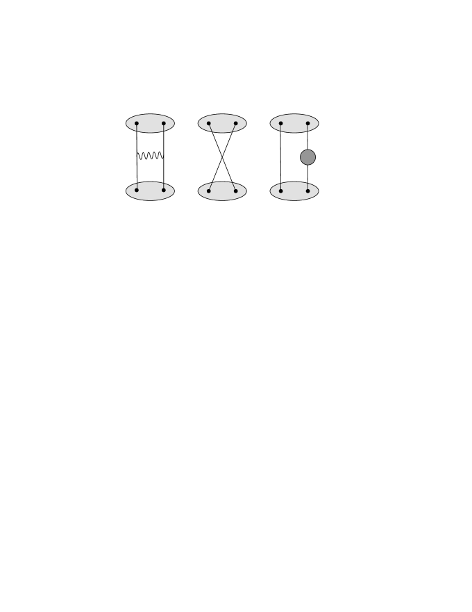
Figure 1: The Feynman diagrams contributing to operator mixing at one-loop.

It turns out that the final result is equal (up to an overall multiplicative coefficient) to the Hamiltonian of a very well studied spin chain problem,

$$\Gamma=\frac{\lambda}{8\pi^{2}}\sum_{\ell=1}^{L}(\mathbb{I}-\mathbb{P}_{\ell,\ell+1})\equiv\frac{\lambda}{16\pi^{2}}\mathcal{H}_{XXX}\,,$$ (1)

where $\mathbb{I}$ is the identity operator and $\mathbb{P}_{\ell,\ell+1}$ the permutation operator that permutes spins (states) on neighbour sites $\ell$ and $\ell+1$. The XXX spin chain is famously integrable and this means that if we know the solution of the 2-body problem we can get the solution of the $n$-body for free. Two $X$’s in the sea of $Z$’s are enough to give the anomalous dimension for $n$ $X$’s in the sea of $Z$’s.

Finally, we would like to end the introduction with the following comment. The result (1) is due entirely to the $F$-terms, since all other contributions ($D$-terms, gluon exchange and self-energy diagram) add up to zero. See Section 4. Some authors refer to this as the “effective vertex”. This is an example of a general property of theories with (extended) supersymmetry and it is known as a non-renormalisation theorem. In its component form it was discovered in DHoker:1998vkc ; DHoker:2001jzy ; Constable:2002hw . However, using superspace it becomes powerful Fiamberti:2008sh ; Sieg:2010tz and makes high-loop computation possible. See Sieg:2010jt for a review.

2 The landscape of 4D theories

Before coming to the technical topics, we will begin our lectures with a big picture section. We will review some basic, but very important facts about 4D supersymmetric theories, which should eventually become clear in the following sections. All possibly unclear or unknown symbols like $\mbox{tr}\phi^{2}$, $m\tilde{Q}Q$ or $\hat{\mathcal{B}}_{1}$ and $\mathcal{E}_{2}$ for the superconformal multiplets will be explained in Sections 4 and 5, respectively.

	vector multiplet	matter multiplet
$\mathcal{N}=4$	adj	not possible
$\mathcal{N}=3$	adj	not possible
$\mathcal{N}=2$	adj	hypermultiplet in any $\mathcal{R}$ of $G$
$\mathcal{N}=1$	adj	chiral multiplet in any $\mathcal{R}$ of $G$
$\mathcal{N}=0$	adj	scalar or fermion in any $\mathcal{R}$ of $G$

Table 1: The landscape of Lagrangian (supersymmetric) theories in four dimensions. For $\mathcal{N}\leq 2$ the matter can be in any representation $\mathcal{R}$ of the gauge group $G$.

$\mathcal{N}=4$ SYM is the maximally supersymmetric theory in four dimensions. It is unique up to the choice of a semi-simple gauge group $G$. $\mathcal{N}=4$ supersymmetry is so strong that it leads to further symmetry enhancement, whereby the theory is also conformal. Dynamics are governed by the $psu(2,2|4)$ algebra. The $\mathcal{N}=4$ SUSY algebra admits only one possible short massless representation, the “vector multiplet” and no “matter multiplet” is allowed. It is an open problem to prove that $\mathcal{N}=4$ SYM with color group $G$ is the only possibility with $\mathcal{N}=4$ supersymmetry and explore if exotic theories exist.

The next case is $\mathcal{N}=3$ and enhances to $\mathcal{N}=4$ SYM when we demand to have a Lagrangian description. Examples of non-Lagrangian $\mathcal{N}=3$ theories were discovered recently Garcia-Etxebarria:2015wns . However in these lectures we will restrict ourselves to theories with a Lagrangian description, for which we have many more tools to employ.

Going down to $\mathcal{N}=2$ supersymmetry we have a huge (largely unexplored and unknown) landscape of theories. There exist conformal and non-conformal theories. For conformal theories with a Lagrangian description we have a complete classification by Bhardwaj and Tachikawa Bhardwaj:2013qia .

Theorem 2.1.

A Lagrangian theory with $\mathcal{N}=2$ supersymmetry is uniquely specified via its quiver. It consists of blobs and lines. Blobs correspond to color groups and lines to hypermultiplets. See figures 2 and 3. Boxes correspond to global/flavor symmetries.

By now we also know many conformal theories with no Lagrangian description. They include generalisations of the Argyres-Seiberg Argyres:2007cn : $T_{N}$ trinion theories Gaiotto:2009we which can be thought of as non-Lagrangian generalisation of “matter multiplets” in class $\mathcal{S}$, as well as Argyres-Douglas theories Argyres:1995jj . This is by no means the complete list. Starting with conformal theories we can obtain non-conformal theories via triggering an $\mathcal{N}=2$ RG flow with $\mathcal{N}=2$ preserving massive deformations.

Theorem 2.2.

Possible mass deformations that preserve $\mathcal{N}=2$ supersymmetry are classified. Using $\mathcal{N}=1$ superspace language they can only be of the form $m\tilde{Q}Q$ and according to superconformal representation theory, they are the highest weight state of the $\hat{\mathcal{B}}_{1}$ superconformal multiplet.

A very good way to obtain many $\mathcal{N}=2$ SCFTs is via orbifolding $\mathcal{N}=4$ SYM. There is an ADE classification of $\mathcal{N}=2$ SCFTs with $SU(N)$ color factors using finite/affine Dynkin diagrams. The simplest possible example is the $\mathbb{Z}_{2}$ orbifold of $\mathcal{N}=4$ SYM, with color group $SU(N)\times SU(N)$, the quiver of which is depicted in Figure 2. The orbifolding procedure gives theories with all the coupling constants equal to each other and to the YM coupling constant of the $\mathcal{N}=4$ mother theory. This is called the orbifold point. To go away from the orbifold point we marginally deform the theory.

Theorem 2.3.

Marginal operators of $\mathcal{N}=2$ SCFTs are classified: for theories with a Lagrangian description they are descendants of $\mbox{tr}\,\phi^{2}$ and according to superconformal representation theory they belong to the $\mathcal{E}_{2}$ superconformal multiplet.

Beginning with the $\mathbb{Z}_{2}$ orbifold of $\mathcal{N}=4$ SYM and adding a marginal deformation we obtain a one parameter family of ${\mathcal{N}}=2$ SCFTs with product gauge group $SU(N)\times SU(N)$ and two exactly marginal couplings $g$ and $\check{g}$. In the rest of the lectures we will refer to it as the interpolating theory and we will use it as our basic example. Once spin chains for this example are understood, the generalisation to any Lagrangian $\mathcal{N}=2$ SCFT is straightforward.

Figure 2: The quiver of the $\mathbb{Z}_{2}$ orbifold of $\mathcal{N}=4$ SYM (the interpolating theory).

Figure 3: The quiver diagram of $\mathcal{N}=2$ SuperConformalQCD (SCQCD) with $N_{f}=2N$.

• For $\check{g}\rightarrow 0$ (ungauging one node) we obtain the $\mathcal{N}=2$ SuperConformalQCD (SCQCD) with $N_{f}=2N$.

• For $\check{g}=g$ we get back to the $\mathbb{Z}_{2}$ orbifold of ${\mathcal{N}}=4$ SYM.

We finish this section by shortly commenting on $\mathcal{N}=1$ theories. The $\mathcal{N}=1$ matter multiplets are chiral thus $\mathcal{N}=1$ quivers have arrows contrary to $\mathcal{N}=2$ theories which are not chiral and whose quivers do not have arrows. Generically, their Lagrangians are not completely specified by the quiver. We also have to specify the superpotential(s). Orbifolding $\mathcal{N}=4$ SYM is a good path to explore the Landscape of $\mathcal{N}=1$ SCFTs which is even more vast and unexplored, than that of $\mathcal{N}=2$ SCFTs. A lot of the properties that we will study for the $\mathcal{N}=2$ orbifold daughters of $\mathcal{N}=4$ SYM go through for $\mathcal{N}=1$ orbifold daughters. A very important class of $\mathcal{N}=1$ orbifold daughters are obtained as $\mathbb{Z}_{\ell}\times\mathbb{Z}_{k}$ orbifolds (class $\mathcal{S}_{k}$ Gaiotto:2015usa ).

To understand the statements above we need to study the representation theory of the supersymmetry algebra and then of the superconformal algebra. We will see that we can learn a lot just from representation theory, even about dynamics.

3 Massless representations of the supersymmetry algebra

To understand all the facts stated in section 2 we begin with a short review of the supersymmety algebra and its massless representations. This is standard textbook material and more details can be found in any supersymmetry book or review. It is worth pointing out that there is a theorem in mathematics (representation theory) which says that there are no non-trivial finite dimensional unitary representations of non-compact groups. This impasse was overcome by Wigner with a trick stemming from his physics intuition. To study representations of the Lorentz/Poincaré group we should go to a reference frame (the rest frame), classify them there and then boost to get everything!

The superalgebra generators $\mathcal{Q}_{\alpha}^{A}$ and $\bar{\mathcal{Q}}_{\dot{\alpha}A}$ have spinor indices $\alpha=1,2$ and $\dot{\alpha}=1,2$ labelling the $SU(2)_{\alpha}\times SU(2)_{\dot{\alpha}}$ Lorentz group and an additional label $A=1,2,...,{\mathcal{N}}$. The algebra they satisfy is

$$\Big{\{}\mathcal{Q}_{\alpha}^{A}\ ,\ \bar{\mathcal{Q}}_{\dot{\beta}B}\Big{\}}\,=\,2\,(\sigma^{\mu})_{\alpha\dot{\beta}}\,P_{\mu}\,\delta^{A}\,_{B}$$ (2)

$$\Big{\{}\mathcal{Q}_{\alpha}^{A}\ ,\ \mathcal{Q}_{\beta}^{B}\Big{\}}\,=\,\epsilon_{\alpha\beta}\,Z^{AB}$$ (3)

with antisymmetric central charges $Z^{AB}=-Z^{BA}$ commuting with all the generators and

$$\left[\mathcal{Q}_{\alpha}^{A}\ ,\ P_{\mu}\right]=0=\left[\bar{\mathcal{Q}}_{\dot{\beta}B}\ ,\ P_{\mu}\right]\,,\qquad\left[\mathcal{L}_{\alpha}\,^{\beta}\ ,\ \mathcal{Q}_{\gamma}^{A}\right]=\delta_{\gamma}\,^{\beta}\mathcal{Q}_{\alpha}^{A}-\frac{1}{2}\delta_{\alpha}\,^{\beta}\mathcal{Q}_{\gamma}^{A}\,,\quad\dots\,.$$ (4)

The $\mathcal{N}=1$ supersymmetry algebra is invariant under a global phase rotation of all supercharges ${Q}_{\alpha}^{A}$, forming a group $U(1)_{r}$.

$$\left[R\,,\,\mathcal{Q}_{\alpha}^{A}\right]=+q\,\mathcal{Q}_{\alpha}^{A}\qquad\left[R\,,\,\bar{\mathcal{Q}}_{\dot{\beta}B}\right]=-q\,\bar{\mathcal{Q}}_{\dot{\beta}B}\,.$$ (5)

In extended $\mathcal{N}>1$ supersymmetry algebras, the different supercharges may also be rotated into one another under the unitary group $SU(\mathcal{N})_{R}$

$$\left[R^{A}\,_{B}\,,\,\mathcal{Q}_{\alpha}^{C}\right]=\delta^{C}\,_{B}\,\,\mathcal{Q}_{\alpha}^{A}-\frac{1}{|\mathcal{N}|}\delta^{A}\,_{B}\,\,\mathcal{Q}_{\alpha}^{C}\,.$$ (6)

These (outer automorphism) symmetries of the supersymmetry algebra are called R-symmetries. In quantum field theories, part or all of these R-symmetries may be broken by anomaly effects.

Concluding our quick presentation of the supersymmetry algebra, it is important to stress that the supersymmetry generators commute with any other bosonic symmetry of the theory like the generators of the color group $G$ or the flavor group $F$,

$$\left[T_{G},\,\mathcal{Q}_{\alpha}^{A}\right]=0=\left[T_{F},\,\mathcal{Q}_{\alpha}^{A}\right]\,.$$ (7)

We now want to classify one particle states and we only care about massless representations as we want to study only SCFTs. As the symmetry algebra is non-compact, there are no finite unitary representations. To study them and classify them we go to the rest frame and then boost to get the full particle content. To get the massless representations of the supersymmetry algebra we let the momentum of the state be $p_{\mu}=(E,\ 0,\ 0,\ E)$. This is just a convenient choice of frame, a null vector, which commutes with the $SO(2)$ little group (the $L_{12}$ generator of the Lorenz algebra). With this choice, the supersymmetry algebra simplifies to

$$\Big{\{}\mathcal{Q}_{\alpha}^{A}\ ,\ \bar{\mathcal{Q}}_{\dot{\beta}B}\Big{\}}=4\,E\,\left(\begin{array}[]{cc}1&0\\ 0&0\end{array}\right)_{\alpha\dot{\beta}}\delta^{A}\,_{B}$$ (8)

which implies that the algebra for the generator $\mathcal{Q}_{2}$ is trivial and will not play any role. The remaining (active) supercharge operators $a^{A}=\frac{1}{2\sqrt{E}}\mathcal{Q}_{1}^{A}$ and $(a^{A})^{\dagger}=\frac{1}{2\sqrt{E}}(\mathcal{Q}_{1}^{A})^{\dagger}=\frac{1}{2\sqrt{E}}\bar{\mathcal{Q}}_{\dot{1}}^{A}$ obey the algebra of $\mathcal{N}$ fermionic creation and annihilation operators (oscillators). Moreover, their commutator with the helicity generator $L_{12}$ teaches us that they raise and lower helicity as follows

• $\left[L_{12}\,,\,\mathcal{Q}_{1}^{A}\right]=-\frac{1}{2}\mathcal{Q}_{1}^{A}$   lowers the helicity by $1/2$

• $\left[L_{12}\,,\,\bar{\mathcal{Q}}_{\dot{1}}^{A}\right]=\frac{1}{2}\bar{\mathcal{Q}}_{\dot{1}}^{A}$  raises the helicity by $1/2$.

Defining a Clifford vacuum as the state killed by all $\mathcal{Q}_{1}^{A}$, we build the massless representation by acting with the helicity raising operators $(\mathcal{Q}_{1}^{A})^{\dagger}$, with $a=1,\cdots,\mathcal{N}$. We label the Clifford vacuum by the helicity $\lambda$.

$$|\lambda\rangle\longrightarrow(\mathcal{Q}_{1}^{A})^{\dagger}|\lambda\rangle=|\lambda+\frac{1}{2}\rangle_{A}\longrightarrow(\mathcal{Q}_{1}^{A})^{\dagger}(\mathcal{Q}_{1}^{B})^{\dagger}|\lambda\rangle=|\lambda+1\rangle_{[A,B]}\longrightarrow\dots\qquad\qquad\qquad\qquad$$

$$\qquad\qquad\qquad\qquad\qquad\qquad\qquad\qquad\qquad\qquad\dots\longrightarrow(\mathcal{Q}_{1}^{1})^{\dagger}\dots(\mathcal{Q}_{1}^{\mathcal{N}})^{\dagger}|\lambda\rangle=|\lambda+\frac{\mathcal{N}}{2}\rangle$$

Due to the antisymmetry of the R-symmetry indices $A,B,\dots=1,\cdots,\mathcal{N}$, the number of states with helicity $\lambda+\frac{k}{2}$ is $\left(\begin{array}[]{c}\mathcal{N}\\ k\\ \end{array}\right)$. Thus, the representation has dimension (total number of states)

$$n=\sum_{k=0}^{\mathcal{N}}\left(\begin{array}[]{c}\mathcal{N}\\ k\\ \end{array}\right)=2^{\mathcal{N}}=2^{\mathcal{N}-1}_{\text{Bosons}}+2^{\mathcal{N}-1}_{\text{Fermions}}\,.$$ (9)

The helicity is flipped by CPT, thus to have a physical theory we need to always have both $|\lambda\rangle$ and $|-\lambda\rangle$ states. We add the CPT conjugate when needed and obtain:

$$n=2^{\mathcal{N}}\times\left\{\begin{array}[]{ll}1&\quad\text{if the multiplet is CPT complete }\\ 2&\quad\text{if the CPT conjugate has to be added}\end{array}\right.$$ (10)

	$\mathcal{N}=1$	$\mathcal{N}=1$	$\mathcal{N}=2$	$\mathcal{N}=2$	$\mathcal{N}=3$	$\mathcal{N}=4$
$\lambda\leq 1$	vector	chiral	vector	hyper	vector	vector
1	1	0	1	0	1	1
$1/2$	1	1	2	1+1	3+1	4
0	0	1+1	1+1	2+2	3+3	6
$-1/2$	1	1	2	1+1	1+3	4
$-1$	1	0	1	0	1	1
Total $\#$	$2\times 2$	$2\times 2$	$2\times 4$	$2\times 4$	$2\times 8$	16

Table 2: The possible massless supersymmetry multiplets in 4D with numbers of massless states as a function of $\mathcal{N}$ and helicity $\lambda\leq 1$.

In Table 2 we summarize all the possible massless multiplets of the 4D supersymmetry algebra. With $\mathcal{N}=3$ and $\mathcal{N}=4$ supersymmetry it is not possible to build matter multiplets with helicity $\lambda<1$. The $\mathcal{N}=3$ and $\mathcal{N}=4$ vector multiplets coincide (after the CPT completion for the $\mathcal{N}=3$), and their quantum field theories are identical (we stress that we demanded that the theory has massless representations). The more inexperienced readers should pay attention to the fact that all the fields which we will use to materialize the content of the $\mathcal{N}=3$ and $\mathcal{N}=4$ vector multiplets should transform in the same way under the color group $G$, i.e. in the adjoint representation of $G$. This fact stems from (7).

The $\mathcal{N}=2$ matter multiplets are called hypermultiplets and they are not chiral due to the $SU(2)_{R}$ R-symmetry of $\mathcal{N}=2$ . We see that to specify an $\mathcal{N}=2$ theory we need to choose the color groups $G$ and the representations $\mathcal{R}$ of $G$ of the hypermultiplets. Again, due to (7) all the elements of the hypermultiplet will transform under the same representation $\mathcal{R}$ of $G$ . All this information we store in a quiver, which consists of blobs and lines. Blobs correspond to color groups and lines to hypermultiplets. As the hypermultiplets are not chiral, the lines do not have arrows. The $\mathcal{N}=1$ matter multiplets are chiral and thus $\mathcal{N}=1$ quivers have arrows.

4 Lagrangians in $\mathcal{N}=1$ superspace language

To understand the dynamics we need to turn to Lagrangians and a very convenient way is to use the $\mathcal{N}=1$ superspace language to construct them.

The $\mathcal{N}=1$ superspace is an extension of the usual Minkowski spacetime by including Grassmann (spinor) coordinates

$$x^{\mu}\rightarrow\left(x^{\mu}\,,\,\theta_{\alpha}\,,\,\bar{\theta}_{\dot{\alpha}}\right)\qquad\alpha,\dot{\alpha}=1,2$$ (11)

As the usual Minkowski coordinates $x^{\mu}$ are generated by acting with translations $P_{\mu}=-i\partial_{\mu}$ on usual functions $f(x+a)=f(x)+a^{\mu}\partial_{\mu}f(x)+\dots$, the new Grassmann coordinates $\theta_{\alpha}$ and $\bar{\theta}_{\dot{\alpha}}$ are generated by acting with the supersymmetry generators $\mathcal{Q}_{\alpha}$ and $\bar{\mathcal{Q}}_{\dot{\beta}}$ of the $\mathcal{N}=1$ supersymmetry algebra on function $f(x,\theta,\bar{\theta})$. Due to the form of the supersymmetry algebra (2), supertranslations (supersymmetry variations) generated by the action of

$$\delta f=\left(\xi\mathcal{Q}+\bar{\xi}\bar{\mathcal{Q}}\right)f(x,\theta,\bar{\theta})$$ (12)

also induce usual translations

$$\left(x^{\mu}\,,\,\theta_{\alpha}\,,\,\bar{\theta}_{\dot{\alpha}}\right)\rightarrow\left(x^{\mu}+i\,\theta\sigma^{\mu}\bar{\xi}-i\,\xi\sigma^{\mu}\bar{\theta}\,,\,\theta_{\alpha}+\xi_{\alpha}\,,\,\bar{\theta}_{\dot{\alpha}}+\bar{\xi}_{\dot{\alpha}}\right)\,.$$ (13)

Thus, the supersymmetry generators are represented as differential operators

$$\mathcal{Q}_{\alpha}=\frac{\partial}{\partial\theta^{\alpha}}-i\,\sigma^{\mu}_{\alpha\dot{\alpha}}\bar{\theta}^{\dot{\alpha}}\partial_{\mu}\,,\qquad\bar{\mathcal{Q}}_{\dot{\alpha}}=\frac{\partial}{\partial\bar{\theta}^{\dot{\alpha}}}+i\,{\theta}^{\alpha}\sigma^{\mu}_{\alpha\dot{\alpha}}\partial_{\mu}\,,$$ (14)

with their anticommutator defined by the supersymmetry algebra (2). We also define supercovariant derivatives

$$D_{\alpha}=\frac{\partial}{\partial\theta^{\alpha}}+i\,\sigma^{\mu}_{\alpha\dot{\alpha}}\bar{\theta}^{\dot{\alpha}}\partial_{\mu}\,,\qquad\bar{D}_{\dot{\alpha}}=\frac{\partial}{\partial\bar{\theta}^{\dot{\alpha}}}-i\,{\theta}^{\alpha}\sigma^{\mu}_{\alpha\dot{\alpha}}\partial_{\mu}\,,$$ (15)

with the property

$$\{D_{\alpha}\,,\,\bar{D}_{\dot{\alpha}}\}=2\sigma^{\mu}_{\alpha\dot{\alpha}}P_{\mu}\qquad\mbox{and}\qquad\{D_{\alpha}\,,\,\mathcal{Q}_{\beta}\}=\{D_{\alpha}\,,\,\bar{\mathcal{Q}}_{\dot{\alpha}}\}=0\,.$$ (16)

Given the fact that the Grassmann coordinates anticommute, a formal power series expansion in $\theta_{\alpha}$ and $\bar{\theta}_{\dot{\alpha}}$ terminates. The most general superfield is

$$\Phi(x,\theta,\bar{\theta})=\phi(x)+\theta\psi(x)+\bar{\theta}\bar{\chi}(x)+\theta^{2}F(x)+\bar{\theta}^{2}G(x)+\theta\sigma^{\mu}\bar{\theta}A_{\mu}(x)+\theta^{2}\bar{\theta}\bar{\lambda}(x)+\bar{\theta}^{2}\theta\rho(x)+\theta^{2}\bar{\theta}^{2}D(x)\,.$$ (17)

This has too many components (degrees of freedom). It corresponds to a reducible representation of the $\mathcal{N}=1$ supersymmetry algebra. To capture the irreducible representations we derived in the previous section we must find ways to impose constraints on the superfield such that they commute (anticommute) with the superalgebra.

We will introduce chiral superfields which are used to describe $\mathcal{N}=1$ matter fields and vector superfields which will materialise the $\mathcal{N}=1$ vector multiplets, which include the gauge fields.

	$\phi$	$\psi_{\alpha}$	$F$	$A_{\mu}$	$\lambda$	$D$
on-shell ($n_{B}=n_{F}=2$)	2	2	0	2	2	0
off-shell ($n_{B}=n_{F}=4$)	2	4	2	3	4	1

Table 3: The field content of $\mathcal{N}=1$ Chiral and $\mathcal{N}=1$ Vector multiplets.

4.1 Chiral superfields

By definition a Chiral superfield obeys the constraint

$$\bar{D}_{\dot{\alpha}}\Phi=0$$ (18)

Noting that $\theta$ and $y^{\mu}=x^{\mu}+i\theta\sigma^{\mu}\bar{\theta}$ are both annihilated by $\bar{D}_{\dot{\alpha}}$, it is easy to solve the constraint (18).

$$\Phi(y,\theta)=\phi(y)+\theta\psi(y)+\theta^{2}F(y)=$$ (19)

$$\Phi(x,\theta,\bar{\theta})=\phi(x)+i\,\theta\sigma^{\mu}\bar{\theta}\partial_{\mu}\phi(x)+\frac{1}{4}\theta^{2}\bar{\theta}^{2}\Box\phi(x)+\theta\psi(x)-i\,\theta^{2}\sigma^{\mu}\bar{\theta}\partial_{\mu}\psi+\theta^{2}F(x)$$

Lagrangians for Chiral superfields and the Kähler potential

A supersymmetry invariant Lagrangian is constructed as the integral of any arbitrary superfield (or combinations of superfields)

$$\mathcal{L}=\int d^{4}\theta\,\mathcal{K}\left(\Phi^{i},\bar{\Phi}^{\bar{i}}\right)\,,\quad\mbox{with}\qquad\delta\mathcal{L}=\partial_{\mu}(\cdots)\,,$$ (20)

where $d^{4}\theta=d^{2}\theta\,d^{2}\bar{\theta}$. What is more, if a term in the Lagrangian is made out of only chiral or only antichiral fields, it is automatically a total derivative

$$\int d^{4}\theta f\left(\Phi\right)=\partial_{\mu}\left(\cdots\right)\,,$$ (21)

that means that the theory is invariant up to transformations (Kähler transformations)

$$\mathcal{K}\rightarrow\mathcal{K}+f\left(\Phi\right)+\bar{f}\left(\bar{\Phi}\right)\,.$$ (22)

Let us begin by looking at the most basic combination of superfields that is supersymmetric, real and has mass dimension four (three properties that our Lagrangian should have)

$$\mathcal{L}_{kin}=\int d^{4}\theta\,\Phi^{i}\bar{\Phi}^{\bar{i}}\,=-\partial_{\mu}\bar{\phi}^{\bar{i}}\partial^{\mu}\phi^{i}+i\,\partial_{\mu}\bar{\psi}^{\bar{i}}\bar{\sigma}^{\mu}\psi^{i}+\bar{F}^{\bar{i}}F^{i}\,.$$ (23)

Doing so we discovered the kinetic terms of $n$ ($i=1,\dots,n$) scalars, Weyl fermions and auxiliary fields, of $n$ chiral off-shell multiplets (see Table 3).

We can think of the scalar fields $\phi^{i}$ as a map from the 4D spacetime to an $n$-complex dimentional target space with complex coordinates $(\phi^{i}\,,\,\bar{\phi}^{\bar{i}})$. The more general function $\mathcal{K}(\Phi^{i},\bar{\Phi}^{\bar{i}})$ is called the Kähler potential and is a real scalar function on the target space. We can use it to define a metric on the target space ($ds^{2}=g_{i\bar{i}}\,d\phi^{i}\,d\bar{\phi}^{\bar{i}}$) and write

$$g_{i\bar{i}}\equiv\partial_{i}\partial_{\bar{i}}\mathcal{K}\qquad\mbox{and}\qquad\mathcal{L}=-g_{i\bar{i}}\partial_{\mu}\bar{\phi}^{\bar{i}}\partial^{\mu}\phi^{i}+i\,g_{i\bar{i}}\partial_{\mu}\bar{\psi}^{\bar{i}}\bar{\sigma}^{\mu}\psi^{i}+g_{i\bar{i}}F^{i}\bar{F}^{\bar{i}}\,.$$ (24)

The target space because of (22) is a Kähler manifold and this is entirely due to $\mathcal{N}=1$ supersymmetry.

The Superpotential and F-terms

The Kähler terms give the kinetic terms when $\mathcal{K}$ is quadratic. For a more general function $\mathcal{K}$ we obtain extra, non-renormalizable, interaction terms with derivatives. For normalisable, non-derivative interaction terms we need holomorphic, superpotential terms

$$\mathcal{L}_{int}=\int d^{2}\theta\,\mathcal{W}\left(\Phi\right)+h.c.=F^{i}\partial_{i}\mathcal{W}\left(\phi\right)+\frac{1}{2}\psi_{i}\psi_{j}\partial_{i}\partial_{j}\mathcal{W}\left(\phi\right)+h.c.\,,$$ (25)

which after integrating out the auxiliary fields

$$\bar{F}^{\bar{i}}=-g^{i\bar{i}}\partial_{i}\mathcal{W}\left(\phi\right)\quad\mbox{and}\quad{F}^{{i}}=-g^{i\bar{i}}\partial_{\bar{i}}\bar{\mathcal{W}}\left(\bar{\phi}\right)$$ (26)

lead to

$$V(\phi)=F^{i}\bar{F}^{\bar{i}}=\sum_{i}\left|g^{i\bar{i}}\partial_{i}\mathcal{W}\left(\phi\right)\right|^{2}\geq 0\,.$$ (27)

The scalar potential $V(\phi)$ that we will derive now is also a function in this target space. Note that the scalar potential in a supersymmetric theory cannot be negative! A simple but important example is the single chiral multiplet theory with $\mathcal{W}\left(\Phi\right)=\frac{1}{2}m\Phi^{2}+\frac{1}{3!}\lambda\Phi^{3}$.

$$\int d^{2}\theta\,\mathcal{W}\left(\Phi\right)=mF\phi+m\psi\psi+\frac{1}{2}\lambda F\phi^{2}+\lambda\psi\psi\phi\,,$$ (28)

which after integrating out the auxiliary field $\bar{F}=-m\phi-\frac{1}{2}\lambda\phi^{2}$ leads to

$$V(\phi)=\bar{F}F=m^{2}\bar{\phi}\phi+\frac{1}{4}\lambda^{2}(\bar{\phi}\phi)^{2}\,.$$ (29)

Note that the Yukawa $\lambda\psi\psi\phi$ and the $\frac{1}{4}\lambda^{2}(\bar{\phi}\phi)^{2}$ coupling are related! This is precisely the reason why in supersymmetric theories miraculous cancellations happen when we compute Feynman diagrams and we never get $\Lambda^{2}$ divergences (only $\log\Lambda$).

4.2 Vector superfield

By definition the Vector or Real superfield obeys

$$V=V^{\dagger}=C+\theta\chi+\bar{\theta}\bar{\chi}+\theta^{2}\varphi+\bar{\theta}^{2}\bar{\varphi}+\theta\sigma^{\mu}\bar{\theta}A_{\mu}$$ (30)

$$+i\,\theta^{2}\bar{\theta}\left(\bar{\lambda}+\frac{1}{2}\bar{\sigma}^{\mu}\partial_{\mu}\chi\right)-i\,\bar{\theta}^{2}\theta\left(\lambda-\frac{1}{2}{\sigma}^{\mu}\partial_{\mu}\bar{\chi}\right)+\frac{1}{2}\theta^{2}\bar{\theta}^{2}\left(D+\Box C\right)\,.$$

This superfield still has too many degrees of freedom ($8_{B}+8_{F}$) to correspond to the massless vector representation of the $\mathcal{N}=1$ supersymmetry algebra. As we will see immediately we will reduce its degrees of freedom via gauge fixing (down to $4_{B}+4_{F}$) which after going on shell will be precisely the correct number ($2_{B}+2_{F}$) in table 3.

The only supersymmetry covariant generalization of the usual $U(1)$ gauge invariance is

$$V\rightarrow V+i\left(\Lambda-\bar{\Lambda}\right)\,,$$ (31)

where $\Lambda$ is a chiral superfield with component expansion

$$\Lambda=\Lambda+\theta\psi_{\Lambda}+\theta^{2}F_{\Lambda}\,.$$ (32)

In components the effect of the gauge transformation is

$$\delta C=i\left(\Lambda-\bar{\Lambda}\right)$$ (33)

$$\delta\chi=i\,\psi_{\Lambda}$$

$$\delta\varphi=i\,F_{\Lambda}$$

$$\delta A_{\mu}=\partial_{\mu}\left(\Lambda+\bar{\Lambda}\right)$$ (34)

$$\delta\lambda=0$$

$$\delta D=0\,.$$

The vector field $A_{\mu}$ transforms as usual with the real part of $\Lambda$. The real scalar $C$ transforms with the imaginary part of $\Lambda$. The abelian gauge symmetry in superspace is larger than the ordinary gauge symmetry. It is $U(1)_{\mathbb{C}}$ instead of $U(1)_{\mathbb{R}}$. More generally, the vector superfield is invariant under the complexification $G_{\mathbb{C}}$ of the gauge group $G$. The component fields $C,\chi,\varphi$ are gauge artifacts and we can gauge them away choosing the “Wess-Zumino gauge”. The WZ gauge fixes the supersymmetric $U(1)_{\mathbb{C}}$ gauge invariance to $U(1)_{\mathbb{R}}$. We can slightly relax the WZ gauge to the “complex gauge” and fix only $\chi=0=\varphi$ and we keep the full complexified $G_{\mathbb{C}}$.

Finally, we just state that for a non abelian gauge theory the gauge transformation is

$$e^{V}\rightarrow e^{-i\bar{\Lambda}}e^{V}e^{i\Lambda}\,.$$ (35)

Lagrangians with vector superfields

To construct a Lagrangian invariant under Lorentz, supersymmetry and gauge transformations it is useful to define the supersymmetric version of the field strength

$$W_{\alpha}=-\bar{D}^{2}(e^{-V}D_{\alpha}e^{V})$$ (36)

that by construction is a chiral superfield

$$W_{\alpha}(y,\theta)=\lambda_{\alpha}(y)+\theta^{\beta}\left(\epsilon_{\beta\alpha}D+F_{\beta\alpha}\right)(y)+\theta^{2}\partial_{\alpha\dot{\alpha}}\bar{\lambda}^{\dot{\alpha}}(y)$$ (37)

and transforms covariantly

$$W_{\alpha}\rightarrow e^{-i\Lambda}W_{\alpha}e^{i\Lambda}\,.$$ (38)

The most obvious real scalar, supersymmetric and gauge invariant combination of $W_{\alpha}$’s with mass dimension four

$$\mathcal{L}=\int d\theta^{2}W^{\alpha}W_{\alpha}+h.c.=-\frac{1}{4}F^{\mu\nu}F_{\mu\nu}+\frac{1}{4}F^{\mu\nu}\tilde{F}_{\mu\nu}+\frac{1}{2}D^{2}-i\,\bar{\lambda}\mathcal{D}_{\mu}\bar{\sigma}^{\mu}\lambda$$ (39)

is the Lagrangian of $\mathcal{N}=1$ SYM, with the covariant derivative $\mathcal{D}_{\mu}=\partial_{\mu}+i\,A_{\mu}$.

Coupling chiral superfields to vector superfields

To construct the theory of a non abelian gauge group $G$ and some fields $\Phi_{i}$ in some representation of $G$,

$$e^{V}\rightarrow e^{-i\bar{\Lambda}}e^{V}e^{i\Lambda}\qquad\mbox{and}\qquad\Phi_{i}\rightarrow e^{-i\Lambda}\Phi_{i}\,,$$ (40)

we can write the gauge invariant generalisation of (23) and (25)

$$\mathcal{L}=\int d^{4}\theta\,\Phi^{\dagger}_{i}e^{V}\Phi_{i}+\int d^{2}\theta\,\mathcal{W}\left(\Phi\right)+h.c.$$ (41)

in addition to the $W^{\alpha}W_{\alpha}$ part. In the WZ gauge

$$\int d^{4}\theta\,\bar{\Phi}_{i}e^{V}\Phi_{i}= -\mathcal{D}_{\mu}\bar{\phi}^{i}\mathcal{D}^{\mu}\phi^{i}+i\,\mathcal{D}_{\mu}\bar{\psi}^{i}\bar{\sigma}^{\mu}\psi^{i}+F^{i}\bar{F}^{i}$$

$$-i\,\bar{\psi}^{i}\,\bar{\lambda}\,\phi^{i}+h.c.+\bar{\phi}^{i}D\phi^{i}\,.$$

Finally, we can derive the scalar potential $V(\phi)=\bar{F}F+\frac{1}{2}D^{2}\geq 0$, as above for chiral fields, and from it obtain the vacuum equations, the $F$- and $D$-flatness conditions

$$\bar{F}^{i}=-\partial_{i}\mathcal{W}\left(\Phi\right)=0\qquad\forall i$$ (43)

$$D^{a}=-\sum_{i}\phi_{i}\,T^{a}\,\bar{\phi}_{i}=0$$

where $a=1,\dots,\mbox{rank}(G)$ and $T^{a}$ are the generators of the Lie algebra $g$.

4.3 $\mathcal{N}=2$ Lagrangians in superspace

The $\mathcal{N}=2$ Vector multiplet contains $(A_{\mu}\ \lambda_{\alpha}^{\mathcal{I}}\ \phi)$, where $\lambda_{\alpha}^{\mathcal{I}}$ are left moving Weyl fermions, and $\phi$ is a complex scalar. Under $SU(2)_{R}$ symmetry, $A_{\mu}$ and $\phi$ are singlets, while $\lambda^{\mathcal{I}}$ transform as a doublet. Using Witten’s diamond diagrams we can depict the field content of an $\mathcal{N}=2$ Vector multiplet as

$$\begin{array}[]{ccc}&A_{\mu}&\\ \lambda^{1}_{\alpha}&&\lambda^{2}_{\alpha}\\ &\phi&\end{array}\,,\quad\lambda^{\mathcal{I}}=\left(\begin{array}[]{c}\lambda^{1}\\ \lambda^{2}\end{array}\right)\,,\quad\mathcal{I}=1,2$$

where the horizontal axis captures the $SU(2)_{R}$ symmetry quantum number while the vertical axis captures the $U(1)_{r}$ symmetry quantum number. In the diamond diagram the diagonals capture $\mathcal{N}=1$ massless representations

$$\mathcal{N}=2\leavevmode\nobreak\ \mbox{Vector}=\leavevmode\nobreak\ (\mathcal{N}=1\leavevmode\nobreak\ \mbox{Vector})\oplus\leavevmode\nobreak\ (\mathcal{N}=1\leavevmode\nobreak\ \mbox{chiral})\,,$$ (44)

or in terms of $\mathcal{N}=1$ superfields $V=\dots+\theta\sigma^{\mu}\bar{\theta}A_{\mu}-i\,\bar{\theta}^{2}\theta\lambda^{1}+\dots+\frac{1}{2}\theta^{2}\bar{\theta}^{2}D$ and $\Phi=\phi+\theta\lambda^{2}+\theta^{2}F$, both in the adjoint representation of the gauge group.

The $\mathcal{N}=2$ hypermultiplet consists of $(\psi_{\alpha}\ \tilde{\psi}_{\alpha}\ Q^{\mathcal{I}})$, where $\psi_{\alpha}$ and $\tilde{\psi}_{\alpha}$ are left moving Weyl fermions, while $Q^{\mathcal{I}}$ are two complex scalars, all transforming in some representation ${\mathcal{R}}$ of $G$. Under $SU(2)_{R}$ symmetry, $\psi$’s are singlets, while $Q^{\mathcal{I}}$ transform as a doublet.

$$\begin{array}[]{ccc}&\psi_{\alpha}&\\ q&&\left(\tilde{q}\right)^{*}\\ &\left(\tilde{\psi}_{\alpha}\right)^{\dagger}&\end{array}\,,\quad Q^{\mathcal{I}}=\left(\begin{array}[]{c}q\\ \tilde{q}^{*}\end{array}\right)\,.$$

In terms of $\mathcal{N}=1$ massless representations,

$$\mathcal{N}=2\leavevmode\nobreak\ \mbox{hyper}\leavevmode\nobreak\ =\leavevmode\nobreak\ (\mathcal{N}=1\leavevmode\nobreak\ \mbox{chiral in}\leavevmode\nobreak\ {\mathcal{R}})\leavevmode\nobreak\ \oplus\leavevmode\nobreak\ (\mathcal{N}=1\leavevmode\nobreak\ \mbox{chiral in}\leavevmode\nobreak\ \bar{\mathcal{R}})\,,\qquad\qquad$$ (45)

$$Q=q+\theta\psi_{\alpha}+\theta^{2}f\quad\mbox{and}\quad\tilde{Q}=\tilde{q}+\theta\tilde{\psi}+\theta^{2}\tilde{f}\,.$$ (46)

Finally, the $\mathcal{N}=4$ Vector multiplet consists of $(A_{\mu}\ \lambda_{\alpha}^{A}\ X^{m})$, where $\lambda_{\alpha}^{A}$, $A=1,\cdots,4$ are left moving Weyl fermions and $X^{m}$, $m=1,\cdots,6$ are real scalars. Under $SU(4)_{R}$ symmetry, $A_{\mu}$ is a singlet, $\lambda_{\alpha}^{A}$ is a 4 and the scalars $X^{i}$ are an antisymmetric 6 $X^{AB}$ representation.

$$\mathcal{N}=4\leavevmode\nobreak\ \mbox{Vector}\leavevmode\nobreak\ = \leavevmode\nobreak\ \left(\mathcal{N}=2\leavevmode\nobreak\ \mbox{Vector}\right)\leavevmode\nobreak\ \oplus\leavevmode\nobreak\ \left(\mathcal{N}=2\leavevmode\nobreak\ \mbox{hyper}\right)\leavevmode\nobreak\$$ (47)

$$= \leavevmode\nobreak\ \left(\mathcal{N}=1\leavevmode\nobreak\ \mbox{Vector}\right)\leavevmode\nobreak\ \oplus\leavevmode\nobreak\ 3\left(\mathcal{N}=1\leavevmode\nobreak\ \mbox{chiral}\right)\,.$$

The $X^{AB}$ are related to the three complex scalars $\phi^{i}$ ($i=1,2,3$) in the three chirals

$$X^{AB}=\left(\begin{array}[]{cc|cc}0&\phi^{1}&\phi^{2}&\phi^{3}\\ -\phi^{1}&0&\phi^{*}_{3}&-\phi^{*}_{2}\\ \hline\cr-\phi^{2}&-\phi^{*}_{3}&0&\phi^{*}_{1}\\ -\phi^{3}&\phi^{*}_{2}&-\phi^{*}_{1}&0\end{array}\right)$$ (48)

and obey the self-duality constraint

$$(X^{AB})^{\dagger}\equiv\bar{X}_{AB}=\frac{1}{2}\epsilon_{ABCD}\,X^{CD}\,.$$ (49)

The $\mathcal{N}=4$ vector multiplet splits into the $\mathcal{N}=2$ Vector multiplet

$$\begin{array}[]{ccc}&A_{\mu}&\\ \lambda^{1}_{\alpha}&&\lambda^{2}_{\alpha}\\ &\phi^{1}&\end{array}\,,$$ (50)

and the $\mathcal{N}=2$ hypermultiplet

$$\begin{array}[]{ccc}&\lambda^{3}_{\alpha}&\\ \phi^{2}&&\phi^{3}\\ &\lambda^{4}_{\alpha}&\end{array}\,.$$ (51)

Using $\mathcal{N}=1$ language we construct the Lagrangians of $\mathcal{N}=2$ or $\mathcal{N}=4$ theories by $(i)$ imposing gauge invariance and $(ii)$ R-symmetry.

The $\mathcal{N}=4$ Lagrangian in $\mathcal{N}=1$ language

To get $\mathcal{N}=4$ SYM we need to use three chiral superfields $\Phi^{i}=\phi^{i}+\theta\psi^{i}+\theta^{2}F^{i}$ that transform in the adjoint representation. This means that the Lagrangian is

$$\mathcal{L}_{\mathcal{N}=4}=\int d^{4}\theta\,\mbox{tr}\left(e^{-gV}\Phi^{\dagger}_{i}e^{gV}\Phi_{i}\right)+\int d\theta^{2}\mbox{tr}\left(W^{\alpha}W_{\alpha}\right)+\int d^{2}\theta\,\mathcal{W}\left(\Phi\right)+h.c.\,.$$ (52)

We will make sure we have $\mathcal{N}=4$ supersymmetry by imposing the $SU({4})$ R-symmetry on an $\mathcal{N}=1$ theory with three chiral and one vector $\mathcal{N}=1$ superfields. In $\mathcal{N}=1$ language, the $SU(4)_{R}$ $R$-symmetry is broken down to an $SU(3)\times U(1)_{R}$ subgroup. The $U(1)_{R}$ is the usual ${\mathcal{N}}=1$ $R$-symmetry, while the $SU(3)$ is a global symmetry. The $SU(3)$ rotates the three chiral superfields leaving $V$ invariant, while under the $U(1)_{R}$ the chiral superfields have charge $2/3$. To derive the Lagrangian all we have to do it to pick the superpotential. $SU(4)_{R}$ $R$-symmetry forbids mass terms. The only holomorphic function that we can pick such that it is $SU(3)$ invariant, holomorphic and leads to a renormalizable Lagrangian is

$$\mathcal{W}=\frac{i\,g}{3!}\epsilon_{ijk}\,\mbox{Tr}\left(\Phi^{i}\Phi^{j}\Phi^{k}\right)\,.$$ (53)

The only ambiguity is the overall coefficient. The way to fix it is by looking at the Yukawa terms: they must appear with the same coefficient so that when we define $\lambda^{A}=(\lambda\ ,\ \psi^{i})$ we get $g\,\bar{X}_{AB}\lambda^{A}\lambda^{B}$. After integrating out the auxiliary fields we get

$${\mathcal{L}}_{\mathcal{N}=4}=\mbox{Tr}\Bigg{[}-\frac{1}{4}F^{\mu\nu}F_{\mu\nu}+i\bar{\lambda}_{A}\bar{\sigma}^{\mu}D_{\mu}\lambda^{A}-\frac{1}{4}D^{\mu}\bar{X}_{AB}D_{\mu}X^{AB}\Bigg{.}$$

$$\Bigg{.}+i\,\sqrt{2}\,g\,X^{AB}\,\bar{\lambda}_{A}\bar{\lambda}_{B}-i\,\sqrt{2}\,g\,\bar{X}_{AB}\lambda^{A}\lambda^{B}-\frac{g^{2}}{4}[X^{AB},X^{CD}]\,[\bar{X}_{CD},\bar{X}_{AB}]\Bigg{]}\,,$$ (54)

where $A,B=1,\dots,4$.

$\mathcal{N}=2$ Lagrangians in $\mathcal{N}=1$ language

For theories with $\mathcal{N}=2$ supersymmetry we can obtain the Lagrangian using $\mathcal{N}=1$ superspace and imposing the $SU(2)_{R}$, gauge invariance and global symmetry invariance. For the vector multiplet the Lagrangian is

$$\mathcal{L}_{\mathcal{N}=2}^{\text{vec}}=\int d^{4}\theta\,\mbox{tr}\left(e^{-gV}\Phi^{\dagger}e^{gV}\Phi\right)+\int d\theta^{2}\mbox{tr}\left(W^{\alpha}W_{\alpha}\right)+h.c.\,.$$ (55)

For a fundamental hypermultiplet the Lagrangian is

$$\mathcal{L}_{\mathcal{N}=2}^{\text{hyper}}=\int d^{4}\theta\,\mbox{tr}\left(\bar{Q}e^{gV}Q+\tilde{Q}e^{-gV}\bar{\tilde{Q}}\right)+\,i\int d\theta^{2}\mbox{tr}\left(g\tilde{Q}\Phi Q\right)+h.c.\,,$$ (56)

while for a bifundamental hypermultiplet

$$\mathcal{L}_{\mathcal{N}=2}^{\text{hyper}}=\int d^{4}\theta\,\mbox{tr}\left(e^{-g_{2}V_{2}}\bar{Q}e^{g_{1}V_{1}}Q+e^{-g_{1}V_{1}}\bar{\tilde{Q}}e^{g_{2}V_{2}}\tilde{Q}\right)$$ (57)

$$\qquad+\,i\int d\theta^{2}\mbox{tr}\left(g_{1}\tilde{Q}\Phi_{1}Q\right)-\,i\int d\theta^{2}\mbox{tr}\left(g_{2}Q\Phi_{2}\tilde{Q}\right)+h.c.\,.$$

The vector multiplet in $\mathcal{N}=2$ superspace

It is desirable to use the formalism in which most of the symmetry is manifest. For the vector multiplet it is possible to use an off-shell $\mathcal{N}=2$ superspace in which it takes a very simple form. Unfortunately, the hypermultipler in off-shell $\mathcal{N}=2$ superspace is more complicated as we have to use an infinite number of auxiliary fields.

In real $\mathbb{R}^{4|8}$ superspace with coordinates $\{x,\theta,\tilde{\theta}\}$ the $\mathcal{N}=2$ vector multiplet can be written using the $\mathcal{N}=2$ chiral superfield strength $\bar{D}_{\dot{\alpha}}\mathcal{W}=0=\bar{\tilde{D}}_{\dot{\alpha}}\mathcal{W}$,

$$\mathcal{W}=\Phi+\tilde{\theta}^{\alpha}W_{\alpha}+\tilde{\theta}^{2}G\,.$$ (58)

Within this formalism, the $\mathcal{N}=2$ SYM classical Lagrangian can be compactly written as

$$\mathcal{L}_{\mathcal{N}=2}^{\text{vec}}=\int d^{2}\theta d^{2}\tilde{\theta}\,\mbox{tr}\big{(}\mathcal{W}^{2}\big{)}=\int d^{2}\theta\,\mbox{tr}\big{(}W^{\alpha}W_{\alpha}\big{)}+\int d^{2}\theta d^{2}\bar{\theta}\,\mbox{tr}\big{(}e^{-V}\bar{\Phi}e^{V}\Phi\big{)}\,.$$ (59)

This is the formalism Seiberg used to show that the beta function of $\mathcal{N}=2$ theories is one-loop exact Seiberg:1988ur .

4.4 Lagrangians of orbifold daughters of $\mathcal{N}=4$ SYM

Consider Type IIB string theory on $\mathbb{R}^{1,3}\times\mathbb{R}^{6}/\Gamma$ with $N$ parallel and coincident D$3$ branes along the $\mathbb{R}^{1,3}$, depicted in Table 4. We parametrise the worldvolume of the D$3$ branes with four real coordinates $X^{0},X^{1},X^{2},X^{3}$, which arrange themselves into the vector representation of the 4D Lorentz group which naturally acts on $\mathbb{R}^{1,3}$. The transverse $\mathbb{R}^{6}$ is parametrised by six real coordinates $X^{4},X^{5},X^{6},X^{7},X^{8},X^{9}$ or alternatively three complex

$$\phi^{1}=\frac{X^{5}+iX^{6}}{\sqrt{2}}\,\quad\phi^{2}=\frac{X^{7}+iX^{8}}{\sqrt{2}}\,,\quad\phi^{3}=\frac{X^{9}+iX^{10}}{\sqrt{2}}$$ (60)

and their hermitian conjugates. In the case without an orbifold singularity ($\Gamma=1$), the open strings stretching between D$3$ branes give rise to ${\mathcal{N}}=4$ SYM theory with gauge group $SU(N)$ on $\mathbb{R}^{1,3}$. The R-symmetry $SU(4)_{R}\simeq SO(6)_{R}$ is identified with the rotations on the transverse $\mathbb{R}^{6}$. In ${\mathcal{N}}=1$ superspace language the theory contains three chiral superfields $\Phi^{1},\Phi^{2},\Phi^{3}$ transforming in the $\mathbf{3}$ of $SU(3)\subset SU(4)_{R}$,

$$\phi^{1}=\Phi^{1}|_{\theta=0}\,,\quad\phi^{2}=\Phi^{2}|_{\theta=0},\quad\phi^{3}=\Phi^{3}|_{\theta=0}\,.$$ (61)

	$X^{0}$	$X^{1}$	$X^{2}$	$X^{3}$	$X^{4}$	$X^{5}$	$X^{6}$	$X^{7}$	$X^{8}$	$X^{9}$
$N$ D$3$	–	–	–	–	$\cdot$	$\cdot$	$\cdot$	$\cdot$	$\cdot$	$\cdot$
$\mathbb{Z}_{\ell}$	$\cdot$	$\cdot$	$\cdot$	$\cdot$	$\cdot$	$\cdot$	$\times$	$\times$	$\times$	$\times$

Table 4: The type IIB setup engineering ${\mathcal{N}}=2$ orbifold daughters of ${\mathcal{N}}=4$ SYM.

The orbifold $\Gamma=\mathbb{Z}_{\ell}$ acts on the coordinates as

$$\Gamma:\left(\phi^{1},\phi^{2},\phi^{3}\right)\mapsto\left(\phi^{1},\omega_{\ell}\phi^{2},\omega_{\ell}^{-1}\phi^{3}\right)\qquad\mbox{with}\qquad\omega_{\ell}:=e^{2\pi i/\ell}\,,$$ (62)

and as the chiral superfields $\Phi^{i}$ are identified with transverse coordinates (61), the action of $\Gamma$ lies diagonally inside $SU(3)$ in the form

$$R=\begin{pmatrix}1&0&0\\ 0&\omega_{\ell}&0\\ 0&0&\omega_{\ell}^{-1}\end{pmatrix}\in SU(2)_{R}\subset SU(3)\,.$$ (63)

Note that $\Gamma$ must also have an action inside the gauge group $SU(N)$ Douglas:1996sw . To visualise this it is useful to go to the Higgs branch by giving vevs to $\phi^{2}=\phi^{3}=v$, see Figure 4.

Figure 4: The $X^{6}X^{7}$ plane in the case of a $\mathbb{Z}_{8}$ orbifold. Higgsing, which corresponds to placing the $N$ D3 branes away from the origin, allow us to clearly see that $k$ images are created. Open strings with their endpoints on the same stack give rise to the fields of the $\mathcal{N}=2$ vector multiplets. Open strings stretching between different stacks give rise to hypermultiplets.

Then, it is clear that for each $D3$ brane, $\ell$ images will be created, as depicted in Figure 4. The action of $\Gamma$ inside the gauge group can be conjugated to an element $\tau$ of the maximal torus $T(SU(N))=U(1)^{N-1}$. After scaling $N\to|\Gamma|N=\ell N$ this action breaks $SU(N\ell)\to SU(N)^{\ell}$. Hence $\tau$ may be written as

$$\tau=\mbox{diag}\left(\mathbb{I},\omega_{\ell}\mathbb{I},\dots,\omega_{\ell}^{\ell-1}\mathbb{I}\right)$$ (64)

where $\mathbb{I}$ denotes the $N\times N$ identity matrix. Quotienting by $\Gamma$ imposes the identifications

$${V}\sim\tau^{\dagger}{V}\tau\,,\quad\Phi^{i}\sim R^{i}_{\leavevmode\nobreak\ j}\tau^{\dagger}\Phi^{j}\tau\,,$$ (65)

which implies that the $\ell N\times\ell N$ matrices of $SU(N\ell)$ break in a adjoint of bifundamentals of the $SU(N)^{\ell}$ quiver

$$V=\begin{pmatrix}V_{(1)}&&&\\ &V_{(2)}&&\\ &&&\ddots&\\ &&&&&V_{(k)}\end{pmatrix}\,,\quad\Phi^{1}=\begin{pmatrix}&Q_{(1)}&\\ &&Q_{(2)}&\\ &&&\ddots&\\ &&&&Q_{(k-1)}\\ Q_{(k)}&&&\end{pmatrix}\,,\quad$$ (66)

$$\Phi^{2}=\begin{pmatrix}&\tilde{Q}_{(k)}&&\\ \tilde{Q}_{(1)}&&&\\ &&\ddots&\\ &&&Q_{(k-1)}\\ \end{pmatrix}\quad\mbox{and}\quad\Phi^{3}=\begin{pmatrix}\Phi_{(1)}&&&\\ &\Phi_{(2)}&&\\ &&&\ddots&\\ &&&&&\Phi_{(k)}\end{pmatrix}\,.$$

After performing these identifications the resulting theory is an ${\mathcal{N}}=2$ elliptic quiver gauge theory with gauge group $SU\left(N\right)^{\ell}$ and superpotential

$$\mathcal{W}_{{\mathcal{N}}=2\,\text{orb.}}=i\,g\,\sum_{n=1}^{\ell}\left(\tilde{Q}_{(n)}\Phi_{(n)}Q_{(n)}-Q_{(n)}\Phi_{(n+1)}\tilde{Q}_{(n)}\right)\,,$$ (67)

which is explicitely obtained by plugging (66) in (53). The important point of this construction is that the ${\mathcal{N}}=2$ elliptic quiver Lagrangian (67) is the same as the ${\mathcal{N}}=4$ one given in (53) (and (52)) with the fields obeying the identification (65).

To remember:

The vector multiplet part of $\mathcal{N}=2$ Lagrangians is identical to the $\mathcal{N}=4$ one. For $\mathcal{N}=2$ orbifold daughters of $\mathcal{N}=4$ SYM every single vertex is inherited from $\mathcal{N}=4$ - we only need to keep track of the color contractions.

The only difference between the $\mathcal{N}=2$ orbifold daughters and their marginal deformaltions is

$$\mathcal{W}_{{\mathcal{N}}=2}=i\,\sum_{n=1}^{\ell}\left(g_{(n)}\tilde{Q}_{(n)}\Phi_{(n)}Q_{(n)}-g_{(n+1)}Q_{(n)}\Phi_{(n+1)}\tilde{Q}_{(n)}\right)\,.$$ (68)

The effective vertex:

In computations of anomalous dimensions (especially when they are done in superspace) non-renormalisation theorems help us. Using $\mathcal{N}=1$ superspace it is easy to see that at least to two loops all the work is done by the superpotential (68). We can think of this as an effective vertex that has the structure

$$\mathbb{I}-\kappa\mathbb{P}_{\ell,\ell+1}\qquad\mbox{or}\qquad\mathbb{I}-\kappa^{-1}\mathbb{P}_{\ell,\ell+1}$$ (69)

with $\kappa=g_{2}/g_{1}$, $\mathbb{I}$ is the identity and $\mathbb{P}_{\ell,\ell+1}$ the permutation operator that permutes spins (states) on neighbour sites $\ell$ and $\ell+1$ as was the case of $\mathcal{N}=4$ SYM we discussed in the introduction, equation (1).

5 Basics of representation theory for the $\mathcal{N}=2$ SCA

We begin this section by quickly reviewing some basic facts about the conformal algebra and it’s representations so that we can smoothly then turn to the supersymmetric case we are interested in. For a complete and pedagogical review we refer the reader to Simmons-Duffin:2016gjk . We will then turn to the SuperConformal algebra (SCA) with $\mathcal{N}=2$ supersymmetry in 4D and its representations. We will follow Dolan:2002zh where all the possible shortening conditions for the ${\mathcal{N}}=2$ superconformal algebra were studied and classified.

5.1 Conformal Algebra and representations

To obtain the conformal algebra, to the Poincaré generators we add the dilatation generator $D$ and the special conformal generator $K_{\mu}$.

$$\left[P_{\mu}\,,\,K_{\nu}\right]=2i\left(\delta_{\mu\nu}D+L_{\mu\nu}\right)\,\,,\qquad\left[D\,,\,P_{\mu}\right]=+\,i\,P_{\mu}\,\,,\qquad\left[D\,,\,K_{\mu}\right]=-\,i\,K_{\mu}\,.$$ (70)

At this stage it is useful to turn from Lorentzian signature to Euclidean and from Minkowski space $\mathbb{R}^{1,3}$ to $\mathbb{R}^{4}$. It is useful to think of $\mathbb{R}^{4}=\mathbb{S}^{3}\times\mathbb{R}$ where the $SO(4)=SU(2)\times SU(2)$ rotations acting on $\mathbb{S}^{3}$ correspond to spin and the radial translations along $\mathbb{R}$ are generated by the dilatation operator $D$. To label states we use their eigenvalues $\Delta,j,\bar{j}$. From (70) we see that $P_{\mu}$ and $K_{\mu}$ are raising and lowering operators of the conformal dimension $\Delta$. Thus, we construct conformal multiplets by defining a vacuum (the highest weight state) that is annihilated by $K_{\mu}|h.w.\rangle=0$ and acting with $P_{\mu}$ we obtain the descendants that fill in the multiplet. Note that the conformal multiplets are non-compact and correspond to infinite dimensional representations.

Using the operator/state correspondence (available in CFTs), the highest weight state $|h.w.\rangle$ corresponds to an operator $\mathcal{O}$ called conformal primary (C.P.). A generic multiplet is labeled by the quantum numbers of the C.P. and is spanned by

$$\mathcal{A}^{\Delta}_{(j,\bar{j})}=\mbox{span}\left\{P_{\mu_{1}}\dots P_{\mu_{n}}\mathcal{O}\right\}$$ (71)

where $\mathcal{O}$ has conformal dimension $\Delta$ and spin $(j,\bar{j})$ corresponding to the state $|h.w.\rangle=|\Delta;j,\bar{j}\rangle$.

To construct unitary representations we impose that the norm of all the states in the multiplet is positive definite $\langle\psi_{i}|\psi_{i}\rangle=|||\psi_{i}\rangle||^{2}\geq 0$. Starting with the highest weight state $|\psi\rangle=|\Delta;j,\bar{j}\rangle$, the first level descendants are four states $P_{\mu}|\psi\rangle=|\Delta+1;j\pm\frac{1}{2},\bar{j}\pm\frac{1}{2}\rangle$. Using (70) we can calculate their norm and find that among them the state with the lowest norm is $|\psi_{1}\rangle=|\Delta+1;j-\frac{1}{2},\bar{j}-\frac{1}{2}\rangle$, with norm

$$\frac{|||\psi_{1}\rangle||^{2}}{2}=\Delta-j-1+\delta_{j,0}-\bar{j}-1+\delta_{\bar{j},0}=\Delta-f(j,\bar{j})\,.$$ (72)

Thus, at level one, unitarity imposes

$$\Delta\geq j+\bar{j}+2 \qquad\mbox{when both}\qquad j\bar{j}\neq 0\,,$$ (73)

$$\Delta\geq j+1 \qquad\mbox{when only}\qquad j\neq 0\quad\mbox{and}\quad\bar{j}=0\,,$$ (74)

$$\Delta\geq\bar{j}+1 \qquad\mbox{when only}\qquad\bar{j}\neq 0\quad\mbox{and}\quad{j}=0\,,$$ (75)

$$\Delta\geq 0 \qquad\mbox{when both}\qquad j=\bar{j}=0\,.$$ (76)

For the C.P. with spin zero we can learn even more by looking for a null vector at level two $P^{2}|\psi\rangle=0$. Using (70) we obtain the measure $||P^{2}|\psi\rangle||\propto\Delta(\Delta-1)$, which means that for $\Delta\in(0,1)$ the measure is $||P^{2}|\psi\rangle||<0$. Thus, unitarity demands that $\Delta=0$ or that $\Delta\geq 1$. There is a gap between $\Delta=0$ and $\Delta\geq 1$. The operator with $\Delta=0$ is the identity operator or the vacuum $|\psi\rangle=|\emptyset\rangle$ of the CFT. The operator with $\Delta=1$ obeys $P^{2}|\psi\rangle=0$ and corresponds to a free scalar obeying the equation of motion $\Box\phi=0$. The null vector at level two is the equation of motion $P^{2}|\psi\rangle=|\Box\phi\rangle=0$. When a C.P. saturates the BPS bound $\Delta=f(j,\bar{j})$ the representation is shorter. We have to through away the states with zero measure and all their descendants.

At this stage we can start making statements about the dynamics of CFTs employing representation theory alone. Short multiplets with $\Delta=f(j,\bar{j})$ can only acquire anomalous dimensions $\Delta=f(j,\bar{j})+\gamma(\lambda)$ (where $\lambda$ is some coupling constant of the theory) only if they can recombine with some other multiplet to make a long multiplet. Recombine means that they can gain back the descendants we had to throw away because of the existence of a null vector. Note that the identity operator can never recombine because of the $\Delta=0$, $\Delta\geq 1$ gap. In the example of the free scalar, its multiplet can recombine and acquire a positive anomalous dimension $\Delta=1+\gamma_{\phi}(\lambda)>1$ if there exists an operator $\Box\phi\propto\lambda\phi^{3}+\dots$ that we can write on the right hand side with $\Delta=3$ at $\lambda=0$ with which $\Box\phi$ can mix under renormalisation. The multiplet of a free scalar is short and is labelled by $\mathcal{B}$. It is obtained from $\mathcal{A}^{\Delta=1}_{(0,0)}$ after removing the equation of motion $\Box\phi=0$ and all its descendants (packed in $\mathcal{A}^{\Delta=3}_{(0,0)}$).

Shortening Conditions			Multiplet
${\mathcal{C}}$		$\Delta=j+\bar{j}+2$	${\mathcal{C}}_{(j,\bar{j})}$
${\mathcal{B}}_{R}$	$j=0$	$\Delta=\bar{j}+1$	${\mathcal{B}}_{(0,\bar{j})}$
${\mathcal{B}}_{L}$	$\bar{j}=0$	$\Delta=j+1$	$\bar{{\mathcal{B}}}_{(j,0)}$
${\mathcal{B}}$	$j=\bar{j}=0$	$\Delta=1$	${\mathcal{B}}$

Table 5: Shortening conditions and short multiplets for the conformal algebra.

At this stage it is better to proceed with more examples. A second familiar case is a free fermion with $\Delta=j+1=\frac{1}{2}+1$ for which the null vector $P^{\alpha\dot{\alpha}}|\psi_{\alpha}\rangle=\partial^{\alpha\dot{\alpha}}\psi_{\alpha}=0$ corresponds to the free Weyl equation of motion, or similarly $P^{\alpha\dot{\alpha}}|\bar{\psi}_{\dot{\alpha}}\rangle=\partial^{\alpha\dot{\alpha}}\bar{\psi}_{\dot{\alpha}}=0$. These multiplets are labeled as $\mathcal{B}_{(1/2,0)}$ and $\mathcal{B}_{(0,1/2)}$ respectively and they can only recombine if there is an operator with dimension $5/2$ and spin $(0,1/2)$ or $(1/2,0)$ such that $\partial^{\alpha\dot{\alpha}}\bar{\psi}_{\dot{\alpha}}\propto\lambda\phi\psi^{\alpha}+\dots$ to fill in the place of the null vector.

A third important example is a conserved current $J_{\mu}$ that corresponds to the state $|3;1/2,1/2\rangle$ with $\Delta=j+\bar{j}+2=1/2+1/2+2=3$ as in (73). The null vector $P|3;1/2,1/2\rangle=|4;0,0\rangle=\partial^{\mu}J_{\mu}=0$ corresponds to the conservation law of the current. In a CFT if there exists an operator $J_{\mu}$ with $\Delta=3$, it is automatically a conserved current and vice versa: if a vector field is conserved it has $\Delta=3$. Conservation implies absence of anomalous dimensions. These shorter representations are denoted as $\mathcal{C}_{(j,\bar{j})}=\mathcal{C}^{\Delta=j+\bar{j}+2}_{(j,\bar{j})}$ with $\mathcal{C}_{(1/2,1/2)}$ being the multiplet of a conserved current.

Finally, the stress energy tensor is the primary for the $\mathcal{C}_{(1,1)}$ multiplet. $T_{\mu\nu}$ corresponds to a state with $|4;1,1\rangle$ and the null vector $P|4;1,1\rangle=|5;1/2,1/2\rangle=\partial^{\mu}T_{\mu\nu}=0$ corresponds to the conservation of the stress energy tensor.

Combining everything we learned above, the only way for an operator to obtain an anomalous dimensions $\Delta=\Delta_{0}+\gamma(\lambda)$ is to recombine. The only way this can be done is if there is another multiplet in the CFT that has conformal dimension and spin which are the same as those of the null vector we had to through away. All the possible ways this can happen are summarised by the recombination rules,

$$\lim_{\gamma\to 0}\left[\mathcal{A}^{\Delta=j+\bar{j}+2+\gamma}_{(j,\bar{j})}\right]=\mathcal{C}_{(j,\bar{j})}\oplus\mathcal{A}^{\Delta=j+\bar{j}+3}_{(j-\frac{1}{2},\bar{j}-\frac{1}{2})}$$ (77)

$$\lim_{\gamma\to 0}\left[\mathcal{A}^{\Delta=j+1+\gamma}_{(j,\bar{j})}\right]=\mathcal{B}^{L}_{j}\oplus\mathcal{C}_{(j-\frac{1}{2},\frac{1}{2})}$$ (78)

$$\lim_{\gamma\to 0}\left[\mathcal{A}^{\Delta=\bar{j}+1+\gamma}_{(j,\bar{j})}\right]=\mathcal{B}^{R}_{\bar{j}}\oplus\mathcal{C}_{(\frac{1}{2},j-\frac{1}{2})}$$ (79)

$$\lim_{\gamma\to 0}\left[\mathcal{A}^{\Delta=1+\gamma}_{(0,0)}\right]=\mathcal{B}\oplus\mathcal{A}^{\Delta=3}_{(0,0)}\,.$$ (80)

Finding ways to explicitly apply these recombination rules to certain CFTs can lead to very impressive results unveiling the dynamical of the theory Rychkov:2015naa .

5.2 SuperConformal Algebra and representations

We begin by recalling that in Lorentzian signature $\bar{\mathcal{Q}}={\mathcal{Q}}^{\dagger}$ is the complex conjugate of $\mathcal{Q}$. In Euclidian they are independent and maybe $\tilde{\mathcal{Q}}$ is a better notation. To write down the superconformal algebra (SCA) in 4D we need for each $\mathcal{Q}_{\alpha}^{A}$ to introduce its $\mathcal{S}^{\alpha}_{A}$ (in radial quantization $\mathcal{S}=\mathcal{Q}^{\dagger}$ the same way $K=P^{\dagger}$)

$$\Big{\{}\mathcal{Q}_{\alpha}^{A}\ ,\ \tilde{\mathcal{Q}}_{\dot{\beta}B}\Big{\}}\,=\,2\,P_{\alpha\dot{\beta}}\,\delta^{A}\,_{B}\qquad\Big{\{}\mathcal{S}^{\alpha}_{A}\ ,\ \tilde{\mathcal{S}}^{\dot{\beta}B}\Big{\}}\,=\,2\,K^{\alpha\dot{\beta}}\,\delta_{A}\,^{B}$$ (81)

$$\Big{\{}\mathcal{Q}_{\alpha}^{A}\ ,\ \mathcal{Q}_{\beta}^{B}\Big{\}}\,=0\qquad\Big{\{}\mathcal{S}^{\alpha}_{A}\ ,\ \mathcal{S}^{\beta}_{B}\Big{\}}\,=0$$ (82)

and most importantly

$$\Big{\{}\mathcal{Q}_{\alpha}^{A}\ ,\ {\mathcal{S}}_{B}^{\beta}\Big{\}}\,=\,4\left(\delta^{A}\,_{B}\left(\mathcal{L}_{\alpha}\,^{\beta}-\frac{1}{2}\delta_{\alpha}\,^{\beta}D\right)-\delta_{\alpha}\,^{\beta}R^{A}\,_{B}\right)\,,$$ (83)

while

$$\Big{\{}\mathcal{Q}_{\alpha}^{A}\ ,\ \tilde{\mathcal{S}}_{B\dot{\beta}}\Big{\}}\,=0=\,\Big{\{}\tilde{\mathcal{Q}}_{A\dot{\alpha}}\ ,\ {\mathcal{S}}_{B}^{\beta}\Big{\}}\,$$ (84)

and

$$\left[D\,,\,\mathcal{Q}_{\alpha}^{A}\right]=+\frac{1}{2}\mathcal{Q}_{\alpha}^{A}\quad,\qquad\left[D\,,\,\tilde{\mathcal{Q}}_{\dot{\alpha}A}\right]=+\frac{1}{2}\tilde{\mathcal{Q}}_{\dot{\alpha}A}$$ (85)

$$\left[D\,,\,\mathcal{S}^{\alpha}_{A}\right]=-\frac{1}{2}\mathcal{S}^{\alpha}_{A}\quad,\qquad\left[D\,,\,\tilde{\mathcal{S}}^{\dot{\alpha}A}\right]=-\frac{1}{2}\tilde{\mathcal{S}}^{\dot{\alpha}A}\,.$$ (86)

Following what we previously learned about the conformal representation theory, from (85) and (86) we see that $\mathcal{Q}$ and $\mathcal{S}$ raise and lower the conformal dimension by $1/2$, respectively. A SuperConformal primary (S.C.P.) is by definition annihilated by all $4\mathcal{N}=8$ conformal supercharges $\mathcal{S}^{\alpha}_{A}$ and $\tilde{\mathcal{S}}^{\dot{\alpha}A}$. A superconformal multiplet is generated by the action of the $4\mathcal{N}=8$ Poincaré supercharges ${\mathcal{Q}}$ and $\tilde{{\mathcal{Q}}}$ on the S.C.P.. A generic long multiplet of the ${\mathcal{N}}=2$ SCA is labeled by the quantum numbers of its S.C.P., the eigenvalues $(\Delta,R,r,j,\bar{j})$ of the Dilatation operator, the Cartan generators of the $SU(2)_{R}\times U(1)_{r}$ R-symmetry and of the Lorentz group, and is denoted by $\mathcal{A}_{R,r(j,\bar{j})}^{\Delta}$. Note that $\mathcal{S},\tilde{\mathcal{S}}|h.w.\rangle=0$ implies that $K|h.w.\rangle=0$ so a S.C.P. is also a primary of the conformal algebra. Moreover, to construct the multiplets we can act with ${\mathcal{Q}}$’s either in a symmetrized way which creates $P$ and thus conformal primaries, or with anti-symmetrized action which keeps us in the finite superconformal multiplet. When some combination of the ${\mathcal{Q}}$’s also annihilates the primary, the corresponding multiplet is shorter. $|R,r\rangle^{h.w.}_{(j,\bar{j})}$ is the highest weight state with eigenvalues $(R,r,j,\bar{j})$ under the Cartan generators of the $SU(2)_{R}\times U(1)_{r}$ R-symmetry and of the Lorentz group. The multiplet built on this state is denoted as $\mathcal{X}_{R,r(j,\bar{j})}$, where the letter $\mathcal{X}$ characterizes the shortening condition. The left column of Table 6 labels the condition. Note that conjugation reverses the signs of $r$, $j$ and $\bar{j}$ in the expression of the conformal dimension.

Shortening Conditions				Multiplet
${\mathcal{B}}_{1}$	${\mathcal{Q}}_{\alpha}^{1}|R,r\rangle^{h.w.}=0$	$j=0$	$\Delta=2R+r$	${\mathcal{B}}_{R,r(0,\bar{j})}$
$\bar{{\mathcal{B}}}_{2}$	$\tilde{{\mathcal{Q}}}_{2\dot{\alpha}}|R,r\rangle^{h.w.}=0$	$\bar{j}=0$	$\Delta=2R-r$	$\bar{{\mathcal{B}}}_{R,r(j,0)}$
${\mathcal{E}}$	${\mathcal{B}}_{1}\cap{\mathcal{B}}_{2}$	$R=0$	$\Delta=r$	${\mathcal{E}}_{r(0,\bar{j})}$
$\bar{\mathcal{E}}$	$\bar{\mathcal{B}}_{1}\cap\bar{\mathcal{B}}_{2}$	$R=0$	$\Delta=-r$	$\bar{\mathcal{E}}_{r(j,0)}$
$\hat{{\mathcal{B}}}$	${\mathcal{B}}_{1}\cap\bar{B}_{2}$	$r=0$, $j,\bar{j}=0$	$\Delta=2R$	$\hat{{\mathcal{B}}}_{R}$
${\mathcal{C}}_{1}$	$\epsilon^{\alpha\beta}{\mathcal{Q}}_{\beta}^{1}|R,r\rangle_{\alpha}^{h.w.}=0$		$\Delta=2+2j+2R+r$	${\mathcal{C}}_{R,r(j,\bar{j})}$
	$({\mathcal{Q}}^{1})^{2}|R,r\rangle^{h.w.}=0$ for $j=0$		$\Delta=2+2R+r$	${\mathcal{C}}_{R,r(0,\bar{j})}$
$\bar{\mathcal{C}}_{2}$	$\epsilon^{\dot{\alpha}\dot{\beta}}\tilde{\mathcal{Q}}_{2\dot{\beta}}|R,r\rangle_{\dot{\alpha}}^{h.w.}=0$		$\Delta=2+2\bar{j}+2R-r$	$\bar{\mathcal{C}}_{R,r(j,\bar{j})}$
	$(\tilde{\mathcal{Q}}_{2})^{2}|R,r\rangle^{h.w.}=0$ for $\bar{j}=0$		$\Delta=2+2R-r$	$\bar{\mathcal{C}}_{R,r(j,0)}$
$\mathcal{F}$	${\mathcal{C}}_{1}\cap{\mathcal{C}}_{2}$	$R=0$	$\Delta=2+2j+r$	${\mathcal{C}}_{0,r(j,\bar{j})}$
$\bar{\mathcal{F}}$	$\bar{\mathcal{C}}_{1}\cap\bar{\mathcal{C}}_{2}$	$R=0$	$\Delta=2+2\bar{j}-r$	$\bar{\mathcal{C}}_{0,r(j,\bar{j})}$
$\hat{{\mathcal{C}}}$	${\mathcal{C}}_{1}\cap\bar{{\mathcal{C}}}_{2}$	$r=\bar{j}-j$	$\Delta=2+2R+j+\bar{j}$	$\hat{{\mathcal{C}}}_{R(j,\bar{j})}$
$\hat{\mathcal{F}}$	${\mathcal{C}}_{1}\cap{\mathcal{C}}_{2}\cap\bar{{\mathcal{C}}}_{1}\cap\bar{{\mathcal{C}}}_{2}$	$R=0,r=\bar{j}-j$	$\Delta=2+j+\bar{j}$	$\hat{{\mathcal{C}}}_{0(j,\bar{j})}$
${\mathcal{D}}$	${\mathcal{B}}_{1}\cap\bar{{\mathcal{C}}_{2}}$	$r=\bar{j}+1$	$\Delta=1+2R+\bar{j}$	${\mathcal{D}}_{R(0,\bar{j})}$
$\bar{\mathcal{D}}$	$\bar{\mathcal{B}}_{2}\cap{{\mathcal{C}}_{1}}$	$-r=j+1$	$\Delta=1+2R+j$	$\bar{\mathcal{D}}_{R(j,0)}$
$\mathcal{G}$	${\mathcal{E}}\cap\bar{{\mathcal{C}}_{2}}$	$r=\bar{j}+1,R=0$	$\Delta=r=1+\bar{j}$	${\mathcal{D}}_{0(0,\bar{j})}$
$\bar{\mathcal{G}}$	$\bar{\mathcal{E}}\cap{{\mathcal{C}}_{1}}$	$-r=j+1,R=0$	$\Delta=-r=1+j$	$\bar{\mathcal{D}}_{0(j,0)}$

Table 6: Shortening conditions and short multiplets for the ${\mathcal{N}}=2$ superconformal algebra.

There are three basic types of shortening ($\mathcal{A}$, ${\mathcal{B}}$ and ${\mathcal{C}}$):

• $\mathcal{A}$-type: No shortening condition: $\mathcal{A}_{R,r(j,\bar{j})}^{\Delta}$ generic long multiplet of the ${\mathcal{N}}=2$ SCA.

• $\mathcal{B}$-type: ${\mathcal{Q}}_{\alpha}|R,r\rangle^{h.w.}=0$ for both $\alpha=+$ and $-$ which means that 2 supercharges kill the highest weight state and is only possible when the highest weight has $j=0$. (or $\bar{\mathcal{B}}$: $\tilde{{\mathcal{Q}}}_{\dot{\alpha}}|R,r\rangle^{h.w.}=0$ only possible when $\bar{j}=0$)
  For $\mathcal{N}=2$ we have two $\mathcal{B}$-type conditions:

  • $\mathcal{B}^{1}$: ${\mathcal{Q}}_{\alpha}^{1}|R,r\rangle^{h.w.}=0$ (or $\bar{\mathcal{B}}_{1}$: $\tilde{{\mathcal{Q}}}_{1\,\dot{\alpha}}|R,r\rangle^{h.w.}=0$)

  • $\mathcal{B}^{2}$: ${\mathcal{Q}}_{\alpha}^{2}|R,r\rangle^{h.w.}=0$ (or $\bar{\mathcal{B}}_{2}$: $\tilde{{\mathcal{Q}}}_{2\,\dot{\alpha}}|R,r\rangle^{h.w.}=0$).

  This type of shortening is $\frac{1}{4}$-BPS (two out of eight ${\mathcal{Q}}$s).

• $\mathcal{C}$-type: $\epsilon^{\alpha\beta}{\mathcal{Q}}_{\beta}|R,r\rangle_{\alpha}^{h.w.}=0$ which means that only one (combination of) supercharge(s) kills the highest weight state. This condition is half as strong as the $\mathcal{B}$-type.
  For $\mathcal{N}=2$ we have two $\mathcal{C}$-type conditions:

  • $\mathcal{C}^{1}$: $\epsilon^{\alpha\beta}{\mathcal{Q}}_{\beta}^{1}|R,r\rangle^{h.w.}=0$ (or $\bar{\mathcal{C}}_{1}$)

  • $\mathcal{C}^{2}$: $\epsilon^{\alpha\beta}{\mathcal{Q}}_{\beta}^{2}|R,r\rangle^{h.w.}=0$ (or $\bar{\mathcal{C}}_{2}$).

  $\mathcal{C}$-type shortening is $\frac{1}{8}$-BPS (one out of eight ${\mathcal{Q}}$s).

Now we can list all the possible combinations of the shortening conditions above. This was done by Dolan:2002zh and we summarise their findings in Table 6. There are three types of multiplets that are $\frac{1}{2}$-BPS. We have in total $\mathcal{Q}_{\alpha}^{A}$, $\tilde{\mathcal{Q}}_{\dot{\beta}B}$: $2\times 2+2\times 2=8$ $Q$s. $\frac{1}{2}$-BPS means that 4 supercharges kill the primary. For these lectures it is important for the reader to at least pay attention to these maximally short, irreducible superconformal representations:

• ${\mathcal{E}}_{r}={\mathcal{E}}_{r(0,0)}$ whose highest weight state is materialised by $\mbox{tr}\bar{\phi}^{\ell}$ with $\ell=r$ (see Table 13 for our convensions) and obeys the shortening condition $\Delta=r$ from $\tilde{\mathcal{Q}}_{{\mathcal{I}}\,\dot{\alpha}}|h.w.\rangle=0$ for all ${\mathcal{I}}$,$\dot{\alpha}$. The scalar $\phi$ is the adjoint complex scalar inside the vector multiplet.

  $$\begin{array}[]{l|cccccc}\Delta\\ \ell&0_{\left(0,0\right)}\\ \ell+\frac{1}{2}&&\frac{1}{2}_{\left(0,\frac{1}{2}\right)}\\ \ell+1&&&0_{\left(0,1\right)},{1_{\left(0,0\right)}}\\ \ell+\frac{3}{2}&&&&\frac{1}{2}_{\left(0,\frac{1}{2}\right)}\\ \ell+2&&&&&&0_{\left(0,0\right)}\\ \hline\cr r&\ell&\ell-\frac{1}{2}&\ell-1&\ell-\frac{3}{2}&&\quad\ell-2\end{array}$$

  The case ${\mathcal{E}}_{1}$ is special as it is the $\mathcal{N}=2$ vector multiplet we discovered above studying the supersymmetry algebra (together with its equations of motion and the auxiliary field). The field content of the $\mathcal{N}=2$ vector multiplet without the equations of motion (after they are removed as they correspond to null vectors) is captured by ${\mathcal{D}}_{0(0,0)}$. The case ${\mathcal{E}}_{2}$ is also important as it contains the Lagrangian of $\mathcal{N}=2$ theories as a descendant. Schematically, the Lagrangian is $\mathcal{L}=Q^{4}\mbox{tr}\phi^{2}$. The highest weight operators of ${\mathcal{E}}_{r}$ parameterise the Coulomb branch (= supersymmetric vacua with $\langle\phi\rangle=a$ and $\langle Q\rangle=0$, important for other applications).

• $\hat{{\mathcal{B}}}_{R}$ whose higherst weight state obeys $\Delta=2R$. This shortening condition requires $r=0$, $j=\bar{j}=0$.

  $$\begin{array}[]{l|ccccc}\Delta\\ 2&&&{1_{\left(0,0\right)}}\\ \frac{5}{2}&&{\frac{1}{2}_{\left(\frac{1}{2},0\right)}}&&\frac{1}{2}_{\left(0,\frac{1}{2}\right)}\\ 3&0_{\left(0,0\right)}&&0_{\left(\frac{1}{2},\frac{1}{2}\right)}&&0_{\left(0,0\right)}\\ \frac{7}{2}&&&\\ 4&&&-0_{\left(0,0\right)}\\ \hline\cr r&1&\frac{1}{2}&0&-\frac{1}{2}&-1\end{array}$$

  For $R=1$, $\Delta=2$ the $\hat{{\mathcal{B}}}_{1}$ multiplet has as its highest weight state the mesonic operator ${\mathcal{M}}_{\mathbf{3}}$ of the $\mathcal{N}=2$ chiral ring (a.k.a. moment map) which is a triplet of the $SU(2)_{R}$. It also contains the flavor current as the vector field with $\Delta=3$ and labeled by $0_{\left(\frac{1}{2},\frac{1}{2}\right)}$. The $\Delta=4$ element denoted as $-0_{\left(0,0\right)}$ corresponds to the conservation of the flavor current. For $R=1/2$ we get the hypermultiplet. The highest weight operators of $\hat{{\mathcal{B}}}_{R}$ parameterise the Higgs branch (= susy vacua with $\langle\phi\rangle=0$ and $\langle Q\rangle\neq 0$).

• $\hat{{\mathcal{C}}}_{0(j,\bar{j})}=\hat{{\mathcal{C}}}_{(j,\bar{j})}$ with shortening condition $\Delta=2+j+\bar{j}$. For $j=\bar{j}=0$ the multiplet $\hat{{\mathcal{C}}}_{0(0,0)}$ contains the stress energy tensor (the state $0_{\left(1,1\right)}$ with $\Delta=4$), the supercurrents (the states $\frac{1}{2}_{\left(1,\frac{1}{2}\right)}$ and $\frac{1}{2}_{\left(\frac{1}{2},1\right)}$ with $\Delta=7/2$) and $SU(2)_{R}$ and the $U(1)_{r}$ R-symmetry currents ($1_{(\frac{1}{2},\frac{1}{2})}$ and $0_{\left(\frac{1}{2},\frac{1}{2}\right)}$ respecively) of the ${\mathcal{N}}=2$ theory.

  $$\begin{array}[]{l|ccccc}\Delta&\\ &&&&\\ 2&&&0_{\left(0,0\right)}&\\ &&&&\\ \frac{5}{2}&&{\frac{1}{2}_{\left(\frac{1}{2},0\right)}}&&\frac{1}{2}_{\left(0,\frac{1}{2}\right)}\\ &&&&\\ 3&{0_{\left(1,0\right)}}&&{{1_{(\frac{1}{2},\frac{1}{2})}}},\,0_{\left(\frac{1}{2},\frac{1}{2}\right)}&&\qquad 0_{\left(0,1\right)}\\ &&&&\\ \frac{7}{2}&&{\frac{1}{2}_{\left(1,\frac{1}{2}\right)}}&&\frac{1}{2}_{\left(\frac{1}{2},1\right)}\\ &&&&\\ 4&&&0_{\left(1,1\right)}\\ &&&-0_{(0,0)},\,-1_{(0,0)}&\\ &&&&\\ \frac{9}{2}&&-\frac{1}{2}_{(\frac{1}{2},0)}&&-\frac{1}{2}_{(0,\frac{1}{2})}\\ &&&&\\ 5&&&-0_{(\frac{1}{2},\frac{1}{2})}&\\ &&&&\\ \hline\cr r&1&\frac{1}{2}&0&-\frac{1}{2}&\qquad-1\end{array}$$ (87)

The $\hat{{\mathcal{C}}}_{(0,0)}$ multiplet has as its primary a “length two” scalar $\mathcal{T}=\bar{\phi}\phi-{\mathcal{M}}_{{\bf{1}}}$. On the other hand in generic theories $\hat{{\mathcal{E}}}_{r}$ and $\hat{{\mathcal{B}}}_{R}$ can have arbitrary length. Moreover, operators that obey these shortening conditions are protected (their anomalous dimensions will be zero) and they will serve as possible vacua of the $\mathcal{N}=2$ spin chains.

There is one more multiplet that is not 1/2 BPS, but 1/4 BPS which we wish to mention here, the $\mathcal{C}_{0,r(0,0)}$ which obeys two $\mathcal{C}$-type conditions and has a primary with $R=0$ and $\Delta=2+r$. The primaries of these multiplets are $\mbox{tr}\left(\mathcal{T}\bar{\phi}^{\ell}\right)$ with $\ell=r$ and are also protected operators. The $\mbox{tr}\left(\mathcal{T}\phi^{\ell}\right)$ operators correspond to the KK tower of a 7D sugra multiplet Gadde:2009dj . They will describe states with a gapless magnon with momentum $p=0$, as we will see in the next section.

As we learned in the previous section the recombination rules of the different short multiplets can teach us lessons concerning the dynamic of the CFTs. The recombination rules for ${\mathcal{N}}=2$ superconformal algebra are Dolan:2002zh

$$\mathcal{A}_{R,r(j,\bar{j})}^{2R+r+2j+2} \simeq {\mathcal{C}}_{R,r(j,\bar{j})}\oplus{\mathcal{C}}_{R+\frac{1}{2},r+\frac{1}{2}(j-\frac{1}{2},\bar{j})}$$ (88)

$$\mathcal{A}_{R,r(j,\bar{j})}^{2R-r+2\bar{j}+2} \simeq \bar{\mathcal{C}}_{R,r(j,\bar{j})}\oplus\bar{\mathcal{C}}_{R+\frac{1}{2},r-\frac{1}{2}(j,\bar{j}-\frac{1}{2})}$$ (89)

$$\mathcal{A}_{R,j-\bar{j}(j,\bar{j})}^{2R+j+\bar{j}+2} \simeq \hat{{\mathcal{C}}}_{R(j,\bar{j})}\oplus\hat{{\mathcal{C}}}_{R+\frac{1}{2}(j-\frac{1}{2},\bar{j})}\oplus\hat{{\mathcal{C}}}_{R+\frac{1}{2}(j,\bar{j}-\frac{1}{2})}\oplus\hat{{\mathcal{C}}}_{R+1(j-\frac{1}{2},\bar{j}-\frac{1}{2})}\,.$$ (90)

Note that the ${\mathcal{E}}_{r}$, and their conjugates, $\hat{{\mathcal{B}}}_{R}$ with $R=1/2,1,3/2$, ${{\mathcal{D}}}_{R}$ with $R=0,1/2$ and their conjugate multiplets can never appear at the right hand side of a recombination rule and thus are protected. The same is true also for ${{\mathcal{B}}}_{\frac{1}{2},r(0,\bar{j})}$ and ${{\mathcal{B}}}_{\frac{1}{2},r(j,0)}$. This way we immediately learn that all Coulomb branch operators are guaranteed to be protected. Similarly all the mesonic operators (moment maps), which generate the Higgs branch, are protected by representation theory alone.

The representations of $\mathcal{N}=4$ superalgebra can be decomposed to $\mathcal{N}=2$ representations so we will not separately present them here, however, we wish to mention that $\mathcal{N}=4$ superalgebra has one $\frac{1}{2}$-BPS multiplet that decomposes to ${\mathcal{N}}=2$ multiplets as Dolan:2002zh

$${\mathcal{B}}_{[0,p,0]}^{\frac{1}{2},\frac{1}{2}} \simeq (p+1)\hat{{\mathcal{B}}}_{\frac{1}{2}p}\oplus{\mathcal{E}}_{p(0,0)}\oplus\bar{{\mathcal{E}}}_{-p(0,0)}$$ (91)

$$\oplus(p-1)\hat{{\mathcal{C}}}_{\frac{1}{2}p-1(0,0)}\oplus p({\mathcal{D}}_{\frac{1}{2}(p-1)(0,0)}\oplus\bar{{\mathcal{D}}}_{\frac{1}{2}(p-1)(0,0)}$$

$$\oplus\bigoplus_{k=1}^{p-2}(k+1)({\mathcal{B}}_{\frac{1}{2}k,p-k(0,0)}\oplus\bar{{\mathcal{B}}}_{\frac{1}{2}k,k-p(0,0)})$$

$$\oplus\bigoplus_{k=0}^{p-3}(k+1)({\mathcal{C}}_{\frac{1}{2}k,p-k-2(0,0)}\oplus\bar{{\mathcal{C}}}_{\frac{1}{2}k,k-p+2(0,0)})$$

$$\oplus\bigoplus_{k=0}^{p-4}\bigoplus_{l=0}^{p-k-4}(k+1)\mathcal{A}_{\frac{1}{2}k,p-k-4-2l(0,0)}^{p}\,.$$

Here the subrscript $[q,p,s]$ denotes the Dynkin labels of $SU(4)_{R}$ while the superscript $\frac{1}{2},\frac{1}{2}$ is there to remind us that the multiplet is $\frac{1}{2}$-BPS. Given the fact that (91) contains ${\mathcal{E}}_{r}$ operators which as we saw above cannot recombine, ${\mathcal{B}}_{[0,p,0]}^{\frac{1}{2},\frac{1}{2}}$ contains the operators that are protected. As we will see in the next sections, operators in ${\mathcal{B}}_{[0,p,0]}^{\frac{1}{2},\frac{1}{2}}$ are possible vacua for the spin chain of $\mathcal{N}=4$ SYM. Similarly, operators in multiplets on the right hand side of (91) are also protected for the corresponding $\mathcal{N}=2$ SCFTs and provide possible vacua for the spin chains of $\mathcal{N}=2$ SCFTs.

The $\frac{1}{2}$-BPS multiplet ${\mathcal{B}}_{[0,1,0]}^{\frac{1}{2},\frac{1}{2}}$ (with $p=1$) plus derivatives is the so called singleton multiplet of $\mathcal{N}=4$ SYM and contains all the single fields of the massless $\mathcal{N}=4$ supersymmetry representation, the $\mathcal{N}=4$ vector multiplet. This representation is used to build up the spin chains of $\mathcal{N}=4$ SYM as the state space for every lattice site is the singleton representation. $\mathcal{N}=2$ SCA has three distinct irreducible singleton representations:

• $\mathcal{V}=\bar{{\mathcal{D}}}_{0}$ the vector multiplet with shortening condition $\Delta=-r=1$

• $\bar{\mathcal{V}}={\mathcal{D}}_{0}$ the conjugate vector multiplet with $\Delta=r=1$

• $\mathcal{H}=\hat{{\mathcal{B}}}_{1/2}$ the hypermultiplet (real representation) with $\Delta=2R=2$.

6 Spin chains of $\mathcal{N}=2$ SCFTs

We now turn to the main purpose of these notes, to construct and study spin chains of $\mathcal{N}=2$ SCFTs. We will always present the features of the spin chains of $\mathcal{N}=2$ SCFTs by comparing them with the features of the spin chains of $\mathcal{N}=4$ SYM which we will assume the reader is familiar with. More details on the the spin chains of $\mathcal{N}=4$ SYM can be found in this volume in the lectures notes of Marius de Leeuw deLeeuw:2019usb , in the Special issue Bombardelli:2016rwb , as well as in the review Beisert:2010jr .

6.1 The Veneziano large N limit

$\mathcal{N}=4$ SYM is known to be integrable in the large $N$ limit. As we learned in Section 3, all the fields of $\mathcal{N}=4$ SYM are in the same $\mathcal{N}=4$ vector multiplet and they are all in the adjoint representation of the color group. Thus, we can use the usual ’t Hooft large $N$ limit which is simply taken by sending the number of colors $N\rightarrow\infty$ and keeping the coupling constant $\lambda=g^{2}_{YM}N$ fixed. Gauge theories with quarks, and in particular $\mathcal{N}=2$ SCFTs, have more parameters, like the number of flavors $N_{f}$ which we also have to specify how to treat the large $N$ limit. There are two possible options. The first is to send $N\rightarrow\infty$ while keeping $N_{f}$ fixed ($N_{f}<<N_{c}$ a.k.a. quenched approximation). For theories with $\mathcal{N}=2$ supersymmetry the beta function is one-loop exact Seiberg:1988ur . For example for $\mathcal{N}=2$ SQCD,

$$\beta=\frac{g^{3}}{16\pi^{2}}(N_{f}-2N_{c})$$ (92)

and thus, if we take the large $N$ limit keeping $N_{f}$ fixed we cannot obtain a CFT.  $\mathcal{N}=2$ SCFTs and in particular SCQCD admits a Veneziano expansion:

$$N=N_{c}\rightarrow\infty\quad\mbox{and}\quad N_{f}\rightarrow\infty\quad\mbox{with}\quad\frac{N_{f}}{N_{c}}=2\quad\mbox{and}\quad\lambda=g^{2}_{YM}N\quad\mbox{kept fixed}.$$

In this case it is useful to use “generalized double line notation” where we draw Feynman diagrams with propagators:

where the black line depicts the color index $a,b,c,d=1,\dots,N$ while the blue dashed line the flavor index $i,j=1,\dots,N_{f}$. Using Witten’s normalization Witten:1979kh where we pull out a factor of $N$ in front of the single trace Lagrangian, each vertex contributes $\lambda N$, each propagator with $1/N$ and each closed color loop (or flavor loop in the Veneziano case) contributes one more $N$. We can quickly convince ourselves via working out a few examples that an important feature of the the Veneziano limit, where $N_{f}\propto N_{c}$ is that the two diagrams below are of the same order: $N^{2}$.

Exactly because in the Veneziano expansion $N\propto N_{f}$, pure “gluball” type operators (with fields only in the vector multiplet) will mix with operators that contain “mesons” (hypers):

$${\mathcal{O}}\sim\mbox{Tr}\left(\phi^{\ell}\bar{\phi}\right)+\mbox{Tr}\left(\phi^{\ell-1}q_{i}\bar{q}^{i}\right)\,,$$

the AdS gravity dual will have closed string states that correspond to these “generalized single-trace” operators Gadde:2009dj

$${\rm Tr}\left(\phi^{k_{1}}{\mathcal{M}}^{\ell_{1}}\phi^{k_{2}}\dots\phi^{k_{n}}{\mathcal{M}}^{\ell_{n}}\right)\,,\quad{\mathcal{M}}_{\;b}^{a}\equiv\sum_{i=1}^{N_{f}}q_{\,\,\,i}^{a}\,\bar{q}_{\,b}^{i}\,,\quad a,b=1,\dots,N\,,\quad i=1,\dots,N_{f}\,,$$

where it is important to stress that when we have a quark $q$ inside the trace, we need to put a $\bar{q}$ right after it and flavor contract them, forming a meson in the adjoint of the color group ${\mathcal{M}}_{\;b}^{a}$, so that we pick up the leading $N$ contribution.

6.2 The state space

We describe the spin chains of ${\mathcal{N}}=4$ SYM by allowing each site to host a “letter” from the unique ultrashort singleton multiplet (= the $\frac{1}{2}$-BPS ${\mathcal{B}}_{[0,1,0]}^{\frac{1}{2},\frac{1}{2}}$ multiplet with an arbitrary number of covariant derivatives $\mathcal{D}_{\alpha\dot{\alpha}}$ on each field.):

$$V=\mathcal{D}^{n}\left(X,\,Y,\,\,Z,\,\bar{X},\,\bar{Y},\,\bar{Z},\,\lambda^{A}_{\alpha},\,\bar{\lambda}_{A}^{\dot{\alpha}},\,\mathcal{F}_{\alpha\beta},\,\bar{\mathcal{F}}_{\dot{\alpha}\dot{\beta}}\right)\,.$$

The state space of every lattice site is $\mathcal{V}_{\ell}=V$ and the total space is obtained simply by the product $\otimes^{L}_{\ell}\mathcal{V}_{\ell}$ over all the lattice sites of the chain that are $L$. These types of spin chains with the same state space on every lattice site are the ones that are mostly studied in the “AdS/CFT integrability” literature.

For ${\mathcal{N}}=2$ SCFTs, obtaining the total space is more complicated. The state space at each lattice site is spanned by

$$\mathcal{V}_{\ell}=\{\mathcal{V}\,,\quad\bar{\mathcal{V}}\,,{\quad\mathcal{H}\,,\quad\bar{\mathcal{H}}}\}$$

where $\mathcal{V}$ and $\mathcal{H}$ now denote the ${\mathcal{D}}_{0(0,0)}$ and $\hat{{\mathcal{B}}}_{1/2}$ ultra short representations of the ${\mathcal{N}}=2$ SCA again with an arbitrary number of derivatives on each field:

$$\mathcal{V}=\mathcal{D}^{n}\left(\phi\,,\,\lambda_{\alpha}^{\mathcal{I}}\,,\,\mathcal{F}_{\alpha\beta}\right)^{a}\,_{b}\quad,\quad\mathcal{H}=\mathcal{D}^{n}\left(Q^{{\mathcal{I}}}\,,\,\psi\,,\,\bar{\tilde{\psi}}\right)^{a}\,_{i}\quad$$

where $a,b=1,\dots,N$ are color indices, while $i=1,\dots,N_{f}$ is a flavor index. However, it is very important to note that due to the large $N$ limit, the color index structure imposes restrictions on the total space $\otimes^{L}_{\ell}\mathcal{V}_{\ell}$:

$$\cdots\,\phi\,\phi\,{Q}\,{\bar{Q}}\,\phi\,\phi\,\cdots\quad=\quad\cdots\,\phi^{a}\,_{b}\,{Q}^{b}\,_{i}\,{\bar{Q}}^{i}\,_{c}\,\phi^{c}\,_{d}\,\cdots$$

where all $a,b,c,d=1,\dots,N$ are color indices. For example $Q\phi$ and $\phi\bar{Q}$ are not allowed in the strict large $N$ limit. Moreover, for the SCQCD every time we have $Q$ we need to put $\bar{Q}$ right after it so that we can flavor contract them. $\bar{Q}Q$ is also not allowed in the strict Veneziano large $N$ limit. The field content of ${\mathcal{N}}=2$ SQCD is summarized in Table 13. We are not aware of an elegant way to describe these restrictions, other than the “orbifolding procedure” which will be one of the important reasons why we find it useful to think of ${\mathcal{N}}=2$ SCQCD as a $\check{g}\to 0$ limit of the interpolating quiver depicted in Figure 2.

Note that in the case of ABJM alternating spin chains have been studied. However the ones we are dealing with now are much more complicated.

6.3 Vacua of the spin chain

As we learned in Section 5 as opposed to ${\mathcal{N}}=4$ SYM for which all protected operators come from the ${\mathcal{B}}_{[0,p,0]}^{\frac{1}{2},\frac{1}{2}}$ multiplet, for ${\mathcal{N}}=2$ SCFTs, we have different types of the possible short ${\mathcal{N}}=2$ SCA multiplets. This means that we have many options for vacua. In the case of $\mathcal{N}=4$ SYM we usually make the choice of vacuum to be the operator $\mbox{tr}Z^{p}$ which is a highest weight state of ${\mathcal{B}}_{[0,p,0]}^{\frac{1}{2},\frac{1}{2}}$ with $\Delta=p$. This is also known as the Berenstein-Maldacena-Nastase (BMN) vacuum (a classical string rotating in $S^{5}$) Berenstein:2002jq . An other prominent choice is the Gubser-Klebanov-Polyakov (GKP) vacuum (classical string rotation in $AdS_{5}$) Gubser:2002tv , with $\Delta-S\propto\log S$, but we will not discuss it here. It may be a good idea to also study excitations of ${\mathcal{N}}=2$ spin chains around this vacuum.

For the $\mathcal{N}=2$ SCQCD the equivalent to the BMN vacuum is the $\mbox{tr}\phi^{\ell}$ vacuum with $\Delta=-r=\ell$ (${\mathcal{E}}_{r}$ shortening condition) which is the only scalar operator that can have an arbitrarily long length and is protected. There is also $\mbox{tr}\left(\mathcal{T}\phi^{\ell}\right)$ but we prefer to view $\mathcal{T}$ as an excitation in the sea of $\phi$s, as we will see in the next section.

For the interpolating quiver depicted in Figure 2 there are (at least) two “reasonable” choices: $\hat{{\mathcal{B}}}_{R}$ and ${\mathcal{E}}_{r}$ which one could select as BMN-like vacuum. The first possibility is the highest weight state of $\hat{{\mathcal{B}}}_{R}$ with $\Delta=2R$ and corresponds to the alternating $\cdots Q\tilde{Q}Q\tilde{Q}Q\tilde{Q}\cdots$ state. The other possibility is ${\mathcal{E}}_{r}$ whose highest weight state has $\Delta=-r$. The $\Delta=-r$ choice of the $\phi$-vacua leads to two inequivalent, but degenerate vacua, one for each vector multiplet of the theory; $\mbox{tr}\phi^{\ell}$ and $\mbox{tr}\check{\phi}^{\ell}$.

In what comes we will concentrate to the $\phi$-vacua. A study of the $Q$-vacuum is not yet available in the literature, but it reveals very interesting properties and is work in progress Zoubos .

6.4 Elementary excitations

Given the complexity of the total state space it is useful for building intuition to begin by considering first the vacua and then states with only one elementary excitation. All multi-particle states will be constructed via scattering elementary excitations.

In the case of $\mathcal{N}=4$ SYM all excitations come from the same ($\mathcal{N}=4$ vector) multiplet. Once we make:

• the choice of vacuum to be $\mbox{tr}Z^{p}$ with $\Delta-p=0$ (= magnon number).

• around which there exist $8_{B}+8_{F}$ elementary excitations with $\Delta-p=1$:
  $\lambda^{A}_{\alpha}$, $X,\bar{X},Y,\bar{Y}$, $\mathcal{D}_{\alpha\dot{\alpha}}$ with $A=1,\dots,4$ the $SU(4)$ index,

• all other $\Delta-p\geq 2$: $\bar{Z}$, $\mathcal{F}_{\alpha\beta}$, $\dots$ excitations correspond to composite states.

At one-loop the dispersion relation of a single excitation in the sea of $Z$’s is

$$E(p)=8\sin^{2}\left(\frac{p}{2}\right)\,.$$ (93)

A derivation of (93) was given in the lectures of Marius de Leeuw deLeeuw:2019usb . An example of a composite state for ${\mathcal{N}}=4$ SYM is $\bar{Z}$, which can be understood as a bound state of $X\bar{X}$ and $Y\bar{Y}$:

$$\cdots\,Z\,Z\,{\color[rgb]{1,0,0}\bar{Z}}\,Z\,Z\,\cdots$$

$$\xhookrightarrow{\quad\mathcal{H}^{(1)}\quad} \cdots\,Z\,Z{\color[rgb]{1,0,0}\left(X\bar{X}+Y\bar{Y}\right)}Z\,Z\,\cdots$$

$$\xhookrightarrow{\quad\mathcal{H}^{(1)}\quad} \cdots\,Z\,Z\,{\color[rgb]{1,0,0}X}\,Z\,{\color[rgb]{1,0,0}\bar{X}}\,Z\,Z\,\cdots$$

Action of the one-loop Dilatation operator (Hamiltonian) $\mathcal{H}^{(1)}$ can turn $\bar{Z}$ to $X\bar{X}$ and $Y\bar{Y}$ which after further actions of the one-loop Dilatation operator can separate from each other and fly apart.

For $\mathcal{N}=2$ SCQCD it also happens that all excitations come from the vector multiplet. This fact is due to the color contractions in the large $N$ limit as we discussed in the previous Subsection 6.2.

• After the choice $\mbox{tr}\phi^{\ell}$ for the vacuum with $\Delta+r=0$,

• there exist $4_{B}+4_{F}$ elementary excitations with $\Delta+r=1$:
  $\lambda^{\mathcal{I}}_{\alpha}$ and $\mathcal{D}_{\alpha\dot{\alpha}}$ with $\mathcal{I}=1,2$ the $SU(2)_{R}$ index.

• All other $\Delta+r\geq 2$: $\mathcal{M}$, $\mathcal{F}_{\alpha\beta}$ $\dots$ are composite states.

Exactly because the $\lambda^{\mathcal{I}}_{\alpha}$s are in the vector multiplet together with $\phi$ there are no funny restrictions on the state space. Moreover, the Feynman diagrams that we need to compute in order to obtain the one-loop Hamiltonian elements and in particular the “effective vertex” are identical to the $\mathcal{N}=4$ SYM ones. Thus, as is the case of the $\mathcal{N}=4$ SYM the elementary excitations have energy:

$$E_{\lambda,\mathcal{D}}(p)=8\sin^{2}\left(\frac{p}{2}\right)\,.$$ (94)

At this stage a comment is in order. The fact that there exist only $4_{B}+4_{F}$ elementary excitations around the BMN vacuum is related to the fact that the gravity dual of $\mathcal{N}=2$ SCQCD is a non-critical string theory Gadde:2009dj .

Our next step is to study of the composite states. At this point the cautious reader may have already understood, that they have the strange property of being dimmers which occupy two sites. For simplicity we will here discuss the one-loop scalar sector of composite dimmers.

One-loop scalar sector of SCQCD:

The sub-sector with only scalar fields is closed only at one-loop. Its neirest neighbor one-loop Hamiltonian reads Gadde:2010zi

$$\mathcal{H}_{\ell,\ell+1}=\bordermatrix{&\phi\phi&Q\bar{Q}&\bar{Q}Q&\phi Q\cr&&&&\cr\phi\phi&2\mathbb{I}+\mathbb{K}-2\mathbb{P}&\sqrt{2}&0&0\cr Q\bar{Q}&\sqrt{2}&2\,(2\mathbb{I}-\mathbb{K})&0&0\cr\bar{Q}Q&0&0&2\mathbb{K}&0\cr\phi Q&0&0&0&2\mathbb{I}}$$

where $\mathbb{I}$ is the identity operator, $\mathbb{P}$ the permutation operator and $\mathbb{K}$ the trace operator and they act on the $SU(2)_{R}$ indices. It is a simple exercise to diagonalise the scalar excitation in the sea of $\phi$’s and get Gadde:2010zi :

$$\mathcal{T}=\bar{\phi}\phi-{\mathcal{M}}_{{\bf{1}}}\quad\mbox{with}\quad E=4\sin^{2}\left(\frac{p}{2}\right)$$ (95)

$$\widetilde{\mathcal{T}}=\bar{\phi}\phi+{\mathcal{M}}_{{\bf{1}}}\quad\mbox{with}\quad E=8$$ (96)

$${\mathcal{M}}_{\bf 3}\quad\mbox{with}\quad E=8$$ (97)

The singlet and the triplet under the $SU(2)_{R}$ mesons are defined in (122). These states of the one-loop scalar sector of SCQCD should be understood as composite (dimeric - they occupy two sites) and have $\Delta+r=2$. To see that $\mathcal{T}$, $\widetilde{\mathcal{T}}$ and ${\mathcal{M}}_{\bf 3}$ can decay to two elementary excitations $\lambda$, we need to use a higher than an one-loop element of the Hamiltonian $\mathcal{H}^{(L>1)}$

$$\cdots\,\phi\,\phi{\color[rgb]{1,0,0}\left(\phi\bar{\phi}\pm\mathcal{M}_{\bf 1}\right)}\phi\,\phi\,\cdots$$

$$\xhookrightarrow{\quad\mathcal{H}^{(L>1)}\quad} \cdots\,\phi\,\phi\,{\color[rgb]{1,0,0}\lambda}\,{\color[rgb]{1,0,0}\lambda}\,\phi\,\phi\,\cdots$$

$$\xhookrightarrow{\quad\mathcal{H}^{(1)}\quad} \cdots\,\phi\,\phi\,{\color[rgb]{1,0,0}\lambda}\,\phi\,{\color[rgb]{1,0,0}\lambda}\,\phi\,\phi\,\cdots$$

The SU(2)_R singlets $\mathcal{T}$ and $\widetilde{\mathcal{T}}$ should be though of as bound states of two $\lambda$s in the singlet representation of SU(2)_R $\epsilon^{\alpha\beta}\lambda^{\mathcal{I}}_{\alpha}\lambda_{{\mathcal{I}}\,\beta}\leftrightarrow\phi\left(\bar{\phi}\phi\pm{\mathcal{M}}_{{\bf{1}}}\right)$. The same can be done with ${\mathcal{M}}_{\bf 3}$ but using two $\lambda$s in the triplet representation of SU(2)_R $\epsilon^{\alpha\beta}\lambda^{1}_{\alpha}\lambda^{2}_{\beta}\leftrightarrow\phi\mathcal{M}_{\mathbf{3}_{+}}$. The scattering to two-loops was studied in Gadde:2012rv .

The reader should also note that, as claimed in the previous section, the $\mbox{tr}\left(\mathcal{T}\phi^{\ell}\right)$ operator (corresponding to the $p=0$ case above) is also a protected operators of $\mathcal{N}=2$ SCQCD.

Scalar impurities in the interpolating theory:

To address the complication that composite magnons in $\mathcal{N}=2$ SCQCD are dimeric, it is useful to think that we are “regularizing” the spin chain of $\mathcal{N}=2$ SCQCD by gauging the flavor symmetry and consider the interpolating orbifold theory (SCQCD ${\check{g}}\to 0$) with $\frac{\check{g}}{g}$ being the regulator. We regularize by inserting $\check{\mathbf{\phi}}$s between the ${Q}$s giving the dimeric impurities the possibility to split:

$$\cdots\,\phi\,\phi\,{\color[rgb]{1,0,0}Q}\,{\color[rgb]{0,0,1}\check{\phi}\,\check{\phi}\,\cdots\,\check{\phi}\,\check{\phi}}\,{\color[rgb]{1,0,0}\bar{Q}}\,\phi\,\phi\,\cdots$$

It is important to remind the reader that in this case we have two degenerate vacua $\mbox{tr}\phi^{\ell}$ and ${\color[rgb]{0,0,1}\mbox{tr}\check{\phi}^{\ell}}$. A single excitation $Q$ in the sea of $\phi$’s interpolates between the two different vacua

$$\dots\,\phi\,\phi\,\phi\,{\color[rgb]{1,0,0}Q}\,{\color[rgb]{0,0,1}\check{\phi}\,\check{\phi}\,\check{\phi}\,\dots}$$ (98)

and we need to necessarily consider an open spin chain, as the scalars $\phi$ and $\check{\phi}$ cannot be color contracted. This is not a gauge invariant operator. Nonetheless, the merit of considering this non-gauge invariant operator is that after gauging the flavor symmetry, the $Q$s can move independently with

$$\Delta+r=1(=\mbox{\it magnon number})\,,$$

thus, they can be interpreted as elementary magnons, bringing us back to $8_{B}+8_{F}$ elementary excitations with $\Delta+r=1$ and an AdS gravity dual that is a critical string theory. The dispersion relation of single excitation $Q$ in the sea of $\phi$’s (which can be computed using the one-loop Hamiltonian (100)) Gadde:2010zi :

$$g^{2}E(p)=2(g-\check{g})^{2}+8\,g\,\check{g}\sin^{2}\left(\frac{p}{2}\right)\,.$$

This dispersion relation has a new feature compared to its ${\mathcal{N}}=4$ SYM counterpart, a mass gap $g^{2}E(p=0)=2(g-\check{g})^{2}$. Interestingly,

• at the orbifold point, where $g=\check{g}$, the mass gap is zero and the dispersion relation becomes identical to the ${\mathcal{N}}=4$ SYM one.

• In the SCQCD limit $\check{g}\rightarrow 0$, $E(p)=2$ and the $Q$’s cannot move any more and the spin chain breaks (the ${\check{\phi}}$s decouple),

in agreement with what we have seen above.

6.5 Important sub-sectors

Sectors with fields only in the ${\mathcal{N}}=2$ vector multiplet:

As we just saw, adjoint fermions $\lambda$ in the sea of $\phi$’s at one-loop have dispersion relation and scattering matrices identical to their ${\mathcal{N}}=4$ SYM counterparts. Precisely the same is true for derivatives $\mathcal{D}$ in the sea of $\phi$’s Liendo:2011xb . These two cases correspond to important closed sub-sectors are known as the $SU(1|1)$ and $SU(1,1)$ sectors, respectively. The $SU(1|1)$ sub-sector is made out of one adjoint scalar and one adjoint fermion both in the $\mathcal{N}=2$ vector multiplet $(\phi,\lambda^{\mathcal{I}=+}_{\alpha=+})$ which are related to each other by the supercharge in the $su(1|1)$ superalgebra. Similarly the non-compact $SU(1,1)$ bosonic sector is made out of operators with $\phi$’s and one kind of derivative, say $\mathcal{D}_{+\dot{+}}$. Both of them have the advantage that are closed to all-loops, simply by charge conservation and due to their symmetry and field content being identical to their ${\mathcal{N}}=4$ SYM counterparts. The reader is invited to draw the Feynman diagrams which would compute the Hamiltonians to explicitly see that, after recalling that the pieces of the action $\mbox{tr}\left(W^{\alpha}W_{\alpha}\right)$ and $\mbox{tr}\left(e^{-V}\bar{\Phi}e^{V}\Phi\right)$ which are used for the computation are identical both in $\mathcal{N}=2$ SCFTs and in $\mathcal{N}=4$ SYM.

The biggest possible sector of operators that is made only out of fields in the ${\mathcal{N}}=2$ vector multiplet and that is closed to all-loops is the $SU(2,1|2)$ sector Pomoni:2013poa :

$$\bigg{\{}\phi\,,\quad\lambda^{\mathcal{I}}_{+}\,,\quad\mathcal{F}_{++}\,,\quad\mathcal{D}_{+\dot{\alpha}}\bigg{\}}\,.$$ (99)

Above, for simplicity we choose $\alpha=+$ in order to get the highest-weight state of the symmetric representation of the $SU(2)_{\alpha}$ part of the Lorentz group. Clearly, all the statements that we will make below hold for any element in the symmetric representation. Let us also recall that $\mathcal{I}=1,2$ is the $SU(2)_{R}$ symmetry index. At one-loop it is immediately clear from the Lagrangian that the scattering of two magnons is identical to scatering in $\mathcal{N}=4$ SYM. And this this sector is integrable with it’s integrability working exactly like in $\mathcal{N}=4$ SYM, a statement that remains true to any loop order Pomoni:2013poa .

In case it is not clear to the reader, we clarify the advantage of thinking about the smallest possible and the largest possible sub-sectors. The smallest possible sub-sectors are easy to prove that they are closed and to see that they are integrable Staudacher:2004tk , as they contain only one type of magnon. Larger sectors contain more magnons and it is harder to show integrability Beisert:2003yb . However, their symmetry (their superalgebra) is large enough to completely fix their Hamiltonian at least to three-loops Beisert:2003jj ; Beisert:2003ys ; Zwiebel:2005er and their all-loop scattering matrix Beisert:2005tm .

Sectors with hypermultiplets:

The “$SU(2)$” sector:

For the interpolating quiver theory there exists a scalar, closed to all-loops sub-sector with $\Delta=2R-r$ and $j=\bar{j}=0$ which is made out of the color adjoints $\phi$ and $\check{\phi}$ and the bifundamentals $Q$ and $\tilde{Q}$. We will refer to it as the “$SU(2)$” sector, because although it resembles a lot the $SU(2)$ sector of $\mathcal{N}=4$, for $\mathcal{N}=2$ gauge theories there is no $SU(2)$ symmetry that rotates the different species into one another.

The one-loop Hamiltonian in this “$SU(2)$” sector is nearest neighbour type

$$\mathcal{H}_{\ell,\ell+1}= \bordermatrix{&\phi\phi&Q\tilde{Q}&\check{\phi}\check{\phi}&\tilde{Q}Q&\phi Q&Q\check{\phi}&\check{\phi}\tilde{Q}&\tilde{Q}\phi\cr&&&&\cr\phi\phi&0&0&0&0&0&0&0&0\cr Q\tilde{Q}&0&0&0&0&0&0&0&0\cr\check{\phi}\check{\phi}&0&0&0&0&0&0&0&0\cr\tilde{Q}Q&0&0&0&0&0&0&0&0\cr\phi Q&0&0&0&0&2&-2\kappa&0&0\cr Q\check{\phi}&0&0&0&0&-2\kappa&2\kappa^{2}&0&0\cr\check{\phi}\tilde{Q}&0&0&0&0&0&0&2\kappa^{2}&-2\kappa\cr\tilde{Q}\phi&0&0&0&0&0&0&-2\kappa&2}$$ (100)

with $\kappa=\frac{\check{g}}{g}$.

As discussed before, there are only two $\Delta=-r$ operators which correspond to the two inequivalent, but degenerate $\phi$-vacua: $\mbox{tr}\left(\phi^{\ell}\right)$ and $\mbox{tr}\left(\check{\phi}^{\ell}\right)$ vacua. In these two $\phi$-vacua we can have two inequivalent $\Delta+r=1$ excitations $Q$ and $\tilde{Q}$ which interpolate between the two different vacua as

$$\cdots\phi\,\phi\,\phi\,Q\,\check{\phi}\,\check{\phi}\,\check{\phi}\cdots$$ (101)

$$\cdots\check{\phi}\,\check{\phi}\,\check{\phi}\,\tilde{Q}\,\phi\,\phi\,\phi\cdots$$

and have the dispersion relation

$$g^{2}E(p)=2(g-\check{g})^{2}+8\,g\,\check{g}\sin^{2}\left(\frac{p}{2}\right)\,.$$ (102)

At the two magnon level $\Delta+r=2$, there exist two different scattering matrices (for the two different boundary conditions),

$$S\quad\mbox{for}\quad\cdots\phi\,\phi\,\phi\,Q\,\check{\phi}\,\check{\phi}\,\check{\phi}\cdots\check{\phi}\,\check{\phi}\,\check{\phi}\,\tilde{Q}\,\phi\,\phi\,\phi\cdots$$

$$\tilde{S}\quad\mbox{for}\quad\cdots\check{\phi}\,\check{\phi}\,\check{\phi}\,\tilde{Q}\,\phi\,\phi\,\phi\cdots\phi\,\phi\,\phi\,Q\,\check{\phi}\,\check{\phi}\,\check{\phi}\cdots \,,$$

which can be derived as in the lectures deLeeuw:2019usb ,

$$S\left(p_{1},p_{2}\right)=-\frac{1+e^{ip_{1}+ip_{2}}-2\kappa e^{ip_{2}}}{1+e^{ip_{1}+ip_{2}}-2\kappa e^{ip_{1}}}$$ (103)

and

$$\tilde{S}\left(p_{1},p_{2}\right)=-\frac{1+e^{ip_{1}+ip_{2}}-2\kappa^{-1}e^{ip_{2}}}{1+e^{ip_{1}+ip_{2}}-2\kappa^{-1}e^{ip_{1}}}\,.$$ (104)

The have the form of the scattering matrix of the XXZ spin chain with anisotropy parameter $\Delta=\kappa$ in the first case and $\Delta=1/\kappa$ in the second. Given the fact that $S\neq\tilde{S}$ the standard YBE is not satisfied

$$S\,\tilde{S}\,S\neq\,\tilde{S}\,S\,\tilde{S}.$$ (105)

This may suggest that $\mathcal{N}=2$ SCFTs are not integrable, at least in the usual (rational) way because already at one-loop (as opposed to $\mathcal{N}=4$ SYM) the scattering matrix in scalar sector Gadde:2010zi did not obey the usual YBE. However, the question of integrability is not so simple to answer and it should be though through more carefully. The XXZ spin chain is a $q$-deformation of the XXX spin chain and also integrable, however, the “$SU(2)$” sector of $\mathcal{N}=2$ SCFTs seems to correspond to a nontrivial (twisted) superposition of two different XXZ spin chains, one with $\Delta=\kappa$ and one with $\Delta=1/\kappa$. This type of $q$-deformed structure seems to remain in higher loops. Via explicit Feynman diagram computations, we have checked that up to 3-loops in Pomoni:2011jj .

At this point we cannot resist but to mention the following fact, which will appear in Zoubos . The results which we have up to now presented are derived for excitations only around the $\phi$-vacua. A study around the $Q$-vacuum for this “$SU(2)$” sector, brings to light the following intriguing results. Allowing for a single $\phi$ excitation to move in the sea of $\cdots Q\tilde{Q}Q\tilde{Q}Q\tilde{Q}\cdots$ and using (100) we can derive the dispersion relation

$$E_{\phi}(p)=2(1+\kappa^{2})-2\sqrt{(1+\kappa^{2})^{2}-2\kappa^{2}\sin^{2}p}\,.$$ (106)

This looks like the dispersion relation of an elliptic system! Already with just an one-loop computation!

The “SU(3$|$2)” sub-sector:

As first discussed in Liendo:2011xb , the bigger sector which includes bifundamental magnons and is similar to the SU(3$|$2) sub-sector of $\mathcal{N}=4$ SYM is

$$\bigg{\{}\phi,\check{\phi},\bar{\psi}_{\dot{\alpha}\hat{\mathcal{I}}=\hat{1}},\bar{\tilde{\psi}}_{\dot{\alpha}\hat{\mathcal{I}}=\hat{1}},Q_{\mathcal{I}\,\hat{\mathcal{I}}=\hat{1}},\bar{Q}_{\mathcal{I}\,\hat{\mathcal{I}}=\hat{1}}\bigg{\}}\,.$$ (107)

The merit of this “SU(3$|$2)” sub-sector is that like for $\mathcal{N}=4$ SYM Beisert:2003jj ; Beisert:2005tm , it is possible to fix the Hamiltonian and the scattering matrix simply by symmetry arguments. We will refer to it as the “SU(3$|$2)” sub-sector to remember that it includes 3 bosons and two fermions. There is no SU(3) symmetry, we have only an SU(2$|$2), which is importantly preserved after the choice of the $\phi$-vacum.

$\bar{\tilde{\psi}}$ $\bar{\psi}$ and $\bar{\psi}$ $\bar{\tilde{\psi}}$ scattering:

The index structure of the fields implies that there cannot be any transmission, $\bar{\tilde{\psi}}$ must always be to the left of $\bar{\psi}$, the process is pure reflection. The one-loop results of Liendo:2011xb for the four different combinations of fields and indices are summarised in Table 7,

Incoming	Sector	Scattering Matrix
$\bar{\tilde{\psi}}\bar{\psi}$	$1_{\dot{\alpha}}\otimes 3_{L}$	$S(p_{1},p_{2},\kappa)$
$\bar{\tilde{\psi}}\bar{\psi}$	$3_{\dot{\alpha}}\otimes 3_{L}$	-1
$\bar{\psi}\bar{\tilde{\psi}}$	$1_{\dot{\alpha}}\otimes 3_{L}$	$S(p_{1},p_{2},1/\kappa)$
$\bar{\psi}\bar{\tilde{\psi}}$	$3_{\dot{\alpha}}\otimes 3_{L}$	-1

Table 7: Components of the S-matrix in the “SU(3$|$2)” sub-sector.

$\bar{\psi}Q$, $Q\bar{\psi}$, $\bar{Q}\bar{\tilde{\psi}}$ and $\bar{\tilde{\psi}}\bar{Q}$ scattering:

These processes are a little bit more interesting because we can have reflection and transmission. Taking into account all four combinations we obtain

Incoming	$T$ and $R$ matrices
$\bar{\psi}Q$	$T(p_{1},p_{2},\kappa),R(p_{1},p_{2},\kappa)$
$Q\bar{\psi}$	$T(p_{1},p_{2},1/\kappa),R(p_{1},p_{2},1/\kappa)$
$\bar{Q}\bar{\tilde{\psi}}$	$T(p_{1},p_{2},\kappa),R(p_{1},p_{2},\kappa)$
$\bar{\tilde{\psi}}\bar{Q}$	$T(p_{1},p_{2},1/\kappa),R(p_{1},p_{2},1/\kappa)$

Table 8: Transmission and reflection coefficients in the “SU(3$|$2)” sub-sector.

where

$$T(p_{1},p_{2}) = -\frac{1-e^{-ip_{2}+ip_{1}}}{\kappa e^{-ip_{2}}+\kappa e^{ip_{1}}-2}\,,$$ (108)

$$R(p_{1},p_{2}) = -\frac{1-\kappa e^{-ip_{2}}-\kappa e^{ip_{1}}+e^{-ip_{2}+ip_{1}}}{\kappa e^{-ip_{2}}+\kappa e^{ip_{1}}-2}\,.$$ (109)

To summarise, the take home message from this section and in particular the Tables 7 and 8 is that:

• the scattering of $\mathcal{V}\,\mathcal{V}$ in the $\phi$-vacuum is identically the same as in ${\mathcal{N}}=4$ SYM,

• the scattering of $\bar{\mathcal{H}}\,\mathcal{H}$ in the $\phi$-vacuum has scattering matrix $S(p_{1},p_{2},\kappa)$, while the $\mathcal{H}\,\bar{\mathcal{H}}$ scattering has $S(p_{1},p_{2},1/\kappa)$.

6.6 All-loop dispersion relation and Scattering Matrix

Beisert’s symmetry argument Beisert:2005tm and the derivation of the all-loop dispersion relations and the all-loop scattering matrix for ${\mathcal{N}}=4$ SYM was given in the lectures of Olof Ohlsson Sax on “Factorised scattering in AdS/CFT” in this school. Here we will only recall the essential elements which render this derivation possible and emphasise the differences between ${\mathcal{N}}=4$ SYM and the ${\mathcal{N}}=2$ SCFTs in which we are interested. The fact that the all-loop dispersion relation and scattering matrix are also possible to derive for ${\mathcal{N}}=2$ SCFTs was shown in Gadde:2010ku , which we will follow and where the interested reader should turn for further details.

	$SU(2)_{\dot{\alpha}}$	$SU(2)_{R}$	$SU(2)_{\alpha}$	$SU(2)_{L}$
$SU(2)_{\dot{\alpha}}$	$\mathcal{L}_{\>\dot{\beta}}^{\dot{\alpha}}$	$\bar{\mathcal{Q}}_{\>\mathcal{J}}^{\dot{\alpha}}$	$\mathcal{P}_{\>\beta}^{\dot{\alpha}}$	$\bar{\mathcal{Q}}_{\>\hat{\mathcal{J}}}^{\dot{\alpha}}$
$SU(2)_{R}$	$\mathcal{S}_{\>\dot{\beta}}^{\mathcal{I}}$	$\mathcal{R}_{\>\mathcal{J}}^{\mathcal{I}}$	$\mathcal{Q}_{\>\beta}^{\mathcal{I}}$	$\mathcal{R}_{\>\hat{\mathcal{J}}}^{\mathcal{I}}$
$SU(2)_{\alpha}$	$\mathcal{P}_{\>\dot{\beta}}^{\alpha}$	$\mathcal{Q}_{\>\mathcal{J}}^{\alpha}$	$\mathcal{L}_{\>\beta}^{\alpha}$	$\mathcal{Q}_{\>\hat{\mathcal{J}}}^{\alpha}$
$SU(2)_{L}$	$\bar{\mathcal{Q}}_{\>\dot{\beta}}^{\hat{\mathcal{I}}}$	$\mathcal{R}_{\>\mathcal{J}}^{\hat{\mathcal{I}}}$	$\mathcal{S}_{\>\beta}^{\hat{\mathcal{I}}}$	$\mathcal{R}_{\>\hat{\mathcal{J}}}^{\hat{\mathcal{I}}}$

Table 9: The generators of $PSU(2,2|4)$.

${\mathcal{N}}=4$ SYM enjoys the full $PSU(2,2|4)$ symmetry, the generators of which are summarised in Table 9, using a perhaps unusual $\mathcal{N}=2$ notation. As we have already discussed in the previous section, to describe magnons we have to first choose a vacuum, around which we will construct the exited states. We will choose the BMN vacuum $\mbox{tr}Z^{\ell}$. This choice of the vacuum breaks half of the symmetries as depicted in the Table 10.

$$PSU(2,2|4)\xrightarrow{\,\text{BMN vac.}\,}PSU(2|2)\times PSU(2|2)\times\mathbb{R}\xrightarrow{\,\text{Beisert}\,}SU(2|2)\times SU(2|2)\times\mathbb{R}$$ (110)

where $\mathbb{R}$ corresponds to the Hamiltonian. Beisert’s idea was to allow for a central extension of the algebra which he showed is enough to fix the form of the dispersion relation and the scattering matrix.

	$SU(2)_{\dot{\alpha}}$	$SU(2)_{R}$	$SU(2)_{\alpha}$	$SU(2)_{L}$
$SU(2)_{\dot{\alpha}}$	$\mathcal{L}_{\>\dot{\beta}}^{\dot{\alpha}}$	$\mathcal{Q}_{\>\mathcal{J}}^{\dot{\alpha}}$	$\mathcal{D}_{\>\beta}^{\dagger\dot{\alpha}}$	$\lambda_{\>\hat{\mathcal{J}}}^{\dagger\dot{\alpha}}$
$SU(2)_{R}$	$\mathcal{S}_{\>\dot{\beta}}^{\mathcal{I}}$	$\mathcal{R}_{\>\mathcal{J}}^{\mathcal{I}}$	$\lambda_{\>\beta}^{\dagger\mathcal{I}}$	$\mathcal{X}_{\>\hat{\mathcal{J}}}^{\dagger\mathcal{I}}$
$SU(2)_{\alpha}$	$\mathcal{D}_{\>\dot{\beta}}^{\alpha}$	$\lambda_{\>\mathcal{J}}^{\alpha}$	$\mathcal{L}_{\>\beta}^{\alpha}$	$\mathcal{Q}_{\>\hat{\mathcal{J}}}^{\alpha}$
$SU(2)_{L}$	$\lambda_{\>\dot{\beta}}^{\hat{\mathcal{I}}}$	$\mathcal{X}_{\>\mathcal{J}}^{\hat{\mathcal{I}}}$	$\mathcal{S}_{\>\beta}^{\hat{\mathcal{I}}}$	$\mathcal{R}_{\>\hat{\mathcal{J}}}^{\hat{\mathcal{I}}}$

Table 10: After choosing the vacuum: broken generators become gapless magnons.

Theorem 6.1.

The broken generators (Goldstone excitations) correspond to “gapless magnons”. These magnons transform in the fundamental of $SU(2|2)$ and have dispersion relation

$$E(p)=\Delta-|r|=\sqrt{1+h\left(g\right)\sin^{2}\left(\frac{p}{2}\right)}$$ (111)

The two-body scattering matrix is fixed by Beisert’s centrally extended $SU(2|2)\times SU(2|2)$ symmetry.

Note that Beisert’s centrally extended $SU(2|2)$ symmetry is enough to fix the dispersion relation and the scattering matrix up to a single function $h(g)$. For ${\mathcal{N}}=4$ SYM, explicit Feynman diagram computations (up to 5-loops Sieg:2010jt ) and string theory computations using AdS/CFT (up to one-loop) give

$$h\left(g\right)=g^{2}\,.$$ (112)

At this moment we wish to stress that there is no way to show (112) in any way other than explicit Feynman diagram computations! Strictly speaking (112) is an input, an assumption, in the ${\mathcal{N}}=4$ SYM integrability business.

	$SU(2)_{\dot{\alpha}}$	$SU(2)_{R}$	$SU(2)_{\alpha}$	$SU(2)_{L}$
$SU(2)_{\dot{\alpha}}$	$\mathcal{L}_{\>\dot{\beta}}^{\dot{\alpha}}$	$\mathcal{Q}_{\>\mathcal{J}}^{\dot{\alpha}}$	$\mathcal{P}_{\>\beta}^{\dot{\alpha}}$
$SU(2)_{R}$	$\mathcal{S}_{\>\dot{\beta}}^{\mathcal{I}}$	$\mathcal{R}_{\>\mathcal{J}}^{\mathcal{I}}$	$\mathcal{Q}_{\>\beta}^{\mathcal{I}}$
$SU(2)_{\alpha}$	$\mathcal{P}_{\>\dot{\beta}}^{\alpha}$	$\mathcal{Q}_{\>\mathcal{J}}^{\alpha}$	$\mathcal{L}_{\>\beta}^{\alpha}$
$SU(2)_{L}$				$\mathcal{R}_{\>\hat{\mathcal{J}}}^{\hat{\mathcal{I}}}$

Table 11: The superconformal algebra plus global symmetry.

For the interpolating quiver (depicted in Figure 2) we begin with the full ${\mathcal{N}}=2$ SCA $SU(2,2|2)$ plus an extra $SU(2)_{L}$ global symmetry (see Appendix A.2). The choice of the $\phi$-vacuum breaks the symmetry down to $SU(2_{\alpha})\times SU(2_{\hat{I}})\times SU(2_{\dot{\alpha}}|2_{I})$ and we obtain the excitations/magnons depicted in Table 12. For generic ${\mathcal{N}}=2$ SCFTs which enjoy just the $SU(2,2|2)$ SCA, after choosing the vacuum to be $\mbox{tr}\phi^{\ell}$ we break the symmetry down to $SU(2_{\dot{\alpha}}|2_{R})\times SU(2)_{\alpha}$. Comparing this with ${\mathcal{N}}=4$ SYM we can say the following.

	$SU(2)_{\dot{\alpha}}$	$SU(2)_{R}$	$SU(2)_{\alpha}$	$SU(2)_{L}$
$SU(2)_{\dot{\alpha}}$	$\mathcal{L}_{\>\dot{\beta}}^{\dot{\alpha}}$	$\mathcal{Q}_{\>\mathcal{J}}^{\dot{\alpha}}$	$\mathcal{\mathcal{D}}_{\>\beta}^{\dagger\dot{\alpha}}$	${\psi_{\>\hat{\mathcal{J}}}^{\dagger\dot{\alpha}}}$
$SU(2)_{R}$	$\mathcal{S}_{\>\dot{\beta}}^{\mathcal{I}}$	$\mathcal{R}_{\>\mathcal{J}}^{\mathcal{I}}$	$\lambda_{\>\beta}^{\dagger\mathcal{I}}$	${\bar{Q}_{\>\hat{\mathcal{J}}}^{\,\mathcal{I}}}$
$SU(2)_{\alpha}$	$\mathcal{D}_{\>\dot{\beta}}^{\alpha}$	$\lambda_{\>\mathcal{J}}^{\alpha}$	$\mathcal{L}_{\>\beta}^{\alpha}$
$SU(2)_{L}$	${\psi_{\>\dot{\beta}}^{\hat{\mathcal{I}}}}$	${Q_{\>\mathcal{J}}^{\hat{\mathcal{I}}}}$		$\mathcal{R}_{\>\hat{\mathcal{J}}}^{\hat{\mathcal{I}}}$

Table 12: After choosing the vacuum: broken generators become gapless magnons and we have some extra magnons that do not come from broken generators.

The broken generators, as is the case for ${\mathcal{N}}=4$ SYM, correspond to Goldstone excitations and lead to gapless magnons. These magnons come from the $\mathcal{N}=2$ vector multiplet and have the same dispersion relation as the excitations of ${\mathcal{N}}=4$ SYM,

$$E_{\lambda,\mathcal{D}}(p)=\sqrt{1+8{\bf g}^{2}\sin^{2}\left(\frac{p}{2}\right)}\,.$$ (113)

Notice that as for the ${\mathcal{N}}=4$ SYM, the centrally extended $SU(2|2)$ symmetry is enough to fix the dispersion relation and the scattering matrix up to a single function ${\bf g}^{2}=f(g,\check{g})=g^{2}+\cdots$ in the case that we are expanding around the $\cdots\phi Q\check{\phi}\cdots$ or ${\bf\check{g}}^{2}=\check{f}(g,\check{g})=\check{g}^{2}+\cdots$ in the case that we are expanding around the $\cdots\check{\phi}\bar{Q}{\phi}\cdots$. These functions are computed up to three-loops in Mitev:2014yba

$$f(g,\check{g})=g^{2}+2\left(\check{g}^{2}-g^{2}\right)\left[6\zeta(3)g^{4}+20\zeta(5)g^{4}\left(\check{g}^{2}+3g^{2}\right)+\cdots\right]\ .$$ (114)

Non-existing generators to start with correpsond to non-Goldstone excitations and thus lead to gapped magnons with dispersion relation

$$E_{Q,\psi}(p)=\sqrt{1+2({\bf g}-\check{{\bf g}})^{2}+8{\bf g}\check{{\bf g}}\sin^{2}\left(\frac{p}{2}\right)}$$ (115)

where again we need to fix two functions $({\bf g}-\check{{\bf g}})^{2}=f_{1}(g,\check{g})=({g}-\check{{g}})^{2}+\cdots$ and ${\bf g}\check{{\bf g}}=f_{2}(g,\check{g})={g}\check{{g}}+\cdots$ via Feynman diagram computations. This is explicitly done up to 3-loops in Pomoni:2011jj .

For the scattering matrix here we will only say that it can also be computed for any $\mathcal{N}=2$ SCFT. After making the choice of vacuum to be $\mbox{tr}\phi^{\ell}$, the scattering matrix of highest weight states in $SU(2)_{\alpha}$ and $SU(2)_{L}$ is fixed by the centrally extended $SU(2|2)$. This was done in Gadde:2010ku . The scattering matrix is also completely fixed up to two functions $f_{1}(g,\check{g})$ and $f_{2}(g,\check{g})$ (as above).

We conclude this section emphasizing that, as we discussed for the one-loop approximation, there exist two different scattering matrices (for the two different boundary conditions)

$$S\quad\mbox{for}\quad\cdots\phi\,\phi\,\phi\,Q\,\check{\phi}\,\check{\phi}\,\check{\phi}\cdots\check{\phi}\,\check{\phi}\,\check{\phi}\,\tilde{Q}\,\phi\,\phi\,\phi\cdots$$

$$\tilde{S}\quad\mbox{for}\quad\cdots\check{\phi}\,\check{\phi}\,\check{\phi}\,\tilde{Q}\,\phi\,\phi\,\phi\cdots\phi\,\phi\,\phi\,Q\,\check{\phi}\,\check{\phi}\,\check{\phi}\cdots$$

with

$$S=S\left(p_{1},p_{2},\kappa\right)\qquad\mbox{and}\qquad\tilde{S}={S}\left(p_{1},p_{2},\kappa^{-1}\right)\,.$$ (116)

The matrices in (116), given the fact that $S\neq\tilde{S}$ do not satisfy the standard YBE

$$S\,\tilde{S}\,S\neq\,\tilde{S}\,S\,\tilde{S}\,,$$ (117)

precisely as we found in the simplest one-loop, “SU(2)” sector.

We finish this section with yet an other intriguing observation. The $SU(2|2)$ scattering matrix of Gadde:2010ku for $Q$ excitations in the sea of $\phi\,\phi\,Q\,\check{\phi}\,\check{\phi}\,\check{\phi}$ has precisely the same form as the quantum double $SU(2|2)$ scattering matrix of Beisert:2016qei , for a certain choice of the quantum deformation parameters. Similarly, $\tilde{Q}$ excitations in the sea of $\check{\phi}\,\check{\phi}\,\tilde{Q}\,\phi\,\phi$ have a scattering matrix which is equal to the quantum double $SU(2|2)$ scattering matrix of Beisert:2016qei , for a slightly different choice ($\kappa\leftrightarrow\kappa^{-1}$) of the quantum deformation parameters. This is very reminiscent of the work of Felder:1994be on elliptic quantum groups and a modified, dynamical Yang-Baxter equation. In fact it looks very possible that this “SU(3$|$2)” sub-sector is governed by a certain elliptic integrable model which is precisely based on an elliptic quantum $SU(2|2)$ and will obey only a dynamical Yang-Baxter equation à la Felder:1994be .

7 Where we stand

7.1 There is an integrable sub-sector (only vector multiplet)

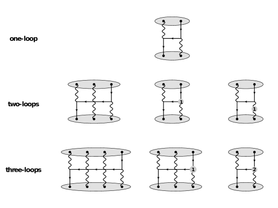
Figure 5: Representatives of the Feynman diagrams we need to compute to three-loops for the Hamiltonian of the $SU(2,1|2)$ sector. The solid lines represents the adjoint $\Phi$ chiral superfield in the $\mathcal{N}=2$ vector multiplet, while the curly lines the real vector superfield $V$.

We already saw that at the one-loop level if we stick to a sub-sector with only fields in one of the vector multiplets, the Hamiltonian is identical to $\mathcal{N}=4$ SYM, $\mathcal{H}^{(1)}_{\mathcal{N}=2}=\mathcal{H}^{(1)}_{\mathcal{N}=4}$. To two-loops (second line in Figure 5) the diagram on the left is also identical to its $\mathcal{N}=4$ SYM counterpart as we only use vertices from the vector multiplet part of the Lagrangian that is identical to its counterpart in $\mathcal{N}=4$ SYM. Leg and vertex corrections can in principle be different by finite corrections, however at one-loop they happen to be identical to $\mathcal{N}=4$ SYM, after an explicit computation Pomoni:2011jj . Thus, to two-loops $\mathcal{H}^{(2)}_{\mathcal{N}=2}=\mathcal{H}^{(2)}_{\mathcal{N}=4}$. Finally, to three-loops (third line in Figure 5) the only diagrams that can be different from their $\mathcal{N}=4$ SYM counterparts, are of the form of the diagram depicted on the right of third line in Figure 5, which contain a two-loop leg or vertex correction and which is proportional to the one-loop Hamiltonian,

$$\mathcal{H}^{(3)}_{\mathcal{N}=2}-\mathcal{H}^{(3)}_{\mathcal{N}=4}\propto\lambda^{3}\mathcal{H}^{(1)}_{\mathcal{N}=4}\quad\Rightarrow\quad\mathcal{H}_{\mathcal{N}=2}=\mathcal{H}_{\mathcal{N}=4}(f(\lambda))+\mathcal{O}(\lambda^{4})\,.$$

This logic can be iterated until we reach the following conclusion Pomoni:2013poa :
Every $\mathcal{N}=2$ SCFT has a purely gluonic $SU(2,1|2)$ sector, integrable in the planar limit with its integrability immediately inherited from $\mathcal{N}=4$ SYM, as its Dilatation operator

$$\mathcal{H}_{\mathcal{N}=2}\left(g\right)=\mathcal{H}_{\mathcal{N}=4}\left(\mathbf{g}\right)\,.$$

The effective coupling:

$$\mathbf{g}^{2}=f(g^{2})=g^{2}+g^{2}\left(Z_{\mathcal{N}=2}-Z_{\mathcal{N}=4}\right)$$

encodes the relative finite renormalization of $g$ and we can either compute it via Feynman diagrams (to some loop order), or we can compute it via Localization by comparing the 1/2-BPS circular Wilson loop, Mitev:2014yba :

$$W_{\mathcal{N}=2}\left({g}^{2}\right)=W_{\mathcal{N}=4}\left(\mathbf{g}^{2}\right)\,,$$

to any order we like. What is more, there is a longer list of observables for which this coupling substitution trick seems to work Fiol:2015spa ; Mitev:2015oty ; Grozin:2015kna ; Gomez:2018usu ; Billo:2019fbi ; Bianchi:2019dlw !

Using AdS/CFT we should understand this function $f(g^{2})$ as the effective string tension $f(g^{2})=T^{2}_{eff}=\left(\frac{R^{4}}{(2\pi\alpha^{\prime})^{2}}\right)_{eff}$. From the gravity dual side we can also check that the coupling substitution rule works to leading order in the strong coupling limit Mitev:2015oty . All in all, AdS/CFT seems to suggests that all that happens in comparison to $\mathcal{N}=4$ SYM is that $f(g^{2})=T^{2}_{eff}$ renormalizes! Thus, it is not too optimistic to hope is that we should be able to obtain any observable which classically resides in the factor $AdS_{5}\times S^{1}$ of the geometry by replacing $g^{2}\rightarrow f(g^{2})$.

It would be very important to have more diagrammatic checks of the diagrammatic argument in Pomoni:2013poa for the purely gluonic SU(2,1$|$2) sector, as well as for the coupling substitution rule Mitev:2014yba (beyond four-loops). What is more, it seems that this coupling substitution rule will also apply to a purely gluonic:

• $SU(2,1|1)$ sub-sector in any $\mathcal{N}=1$ superconformal gauge theories Carstensen and

• $SU(2,1)$ sub-sector in any $\mathcal{N}=0$ superconformal gauge theories

which would be worth exploring both with explicit Feynman diagram computations, as well as with symmetry arguments ( à la Beisert). For ${\mathcal{N}}=1$ SCFTs in class $\mathcal{S}_{k}$ most of the results that we have for ${\mathcal{N}}=2$ SCFTs immediately go though. See Sadri:2005gi for a first attempt with very interesting applications.

7.2 Orbifolds of $\mathcal{N}=4$ SYM are integrable (with hypers)

In this section we will present a very short review of the work of Beisert:2005he . Beisert and Roiban where able to show that the orbifold daughters of $\mathcal{N}=4$ SYM we introduced in Section 4.4 are integrable. Integrability is also there for more general orbifolds Solovyov:2007pw , at the orbifold point, as well as for orbifolds that preserve $\mathcal{N}=1$ supersymmetry. Discovering integrability for orbifold daughters of $\mathcal{N}=4$ SYM is done through the following steps:

• First we need to define a twist operator which commutes with the fields in the $\mathcal{N}=2$ vector multiplet, but produces a phase for the “twisted” fields in the hypermultiplet (recall equation (65)).

• In the process of computing the anomalous dimensions of untwisted operators, no twist operator is involved and the orbifold Hamiltonian is the same as in $\mathcal{N}=4$, as should be clear from the discussion in in Section 4.4. Thus, the asymptotic Bethe ansatz equations for untwisted operators are the same as for $\mathcal{N}=4$ SYM.

• When computing the anomalous dimensions of twisted operators, a twist operator $\gamma$ is present but can and should be shifted using the commutation relation (65) as

  $$X\,\gamma=e^{2\pi is_{X}/2}\gamma X\,.$$ (118)

  This equation determines the phase shift for exchanging $\gamma$ with $X$, which $s_{X}$ given by the $R$-symmetry of the field $X$, as in equation (65).

• We now should think of $\gamma$ as one more excitation which does not have a spectral parameter. Then, the scattering matrix of it with any other excitation is

  $$S_{X,\gamma}=\frac{1}{S_{\gamma,X}}=e^{2\pi is_{X}/2}$$ (119)

• The Bethe equations are just a product of all the scattering matrices (equations (3.8) in Beisert:2005he ) and schematically look like:

  $$\prod^{all\,exitations}\prod^{M}S=1$$ (120)

  where the product $\prod^{M}$ runs over the number of magnons $M$ which our operator contains and the product $\prod^{all\,exitations}$ over all possible types including $\gamma$.

7.3 Marginal deformations away from the orbifold point

Summarising what we have seen in the sections before, there are some sectors (with only fields in the vector multiplets) that are integrable, and some sectors which at least naively are not, because the the standard YBE is not satisfied. These are sectors that include hypermultiplets and thus will include twisted operators.

Up to now nobody has tried to write down something like (120) and to see if they would produce the correct anomalous dimensions, even at one-loop. It is very possible that if we can define a twist operator which depends on the coupling constants (the marginal deformations away from the orbifold point) of the form

$$X\,\gamma=\kappa^{\pm}\,e^{2\pi is_{X}/2}\gamma X$$ (121)

we could succeed in having an equation of the form of (120). This idea brings to mind and should be combined with the work of Mansson:2008xv ; Dlamini:2016aaa ; Dlamini:2019zuk .

It is important to stress that even for $\mathcal{N}=4$ SYM the all-loop Beisert (spin-chain) $SU(2|2)$ S-matrix does not always satisfy the standard YBE Arutyunov:2006yd . Although for the world-sheet $SU(2|2)$ S-matrix the usual YBE is satisfied, showing integrability for the spin-chain of $\mathcal{N}=4$ requires the use of the twisted Zamolodchikov-Faddeev (ZF) algebra and only the twisted YBE is satisfied Arutyunov:2006yd . The reason for that is that single magnon states can not simply be tensored to give two-magnon states and that the transformation of the ZF basis involves the momentum operator. A similar, but more complicated approach seems to be needed for the spin chains of $\mathcal{N}=2$ SCFTs.

7.4 Fixing the dilatation operator just with symmetry arguments

Even though there was no time in these lectures to cover this very interesting direction, we wish to just let the reader know that the $\mathcal{N}=2$ and $\mathcal{N}=1$ SCAs are powerful enough to completely fix the “complete one-loop Hamiltonians”. From Liendo:2011xb ; Liendo:2011wc we know how to get the complete one-loop hamiltonians for $\mathcal{N}=2$ and $\mathcal{N}=1$ SCFTs purely using representation theory. Amazingly, even $\mathcal{N}=0$ Hamiltonians can be fixed only using the conformal representation theory plus some minimal dynamical input (the multiplet recombination in (80)) Liendo:2017wsn !

It is also possible to obtain higher loops Hamiltonians simply via using the superconformal algebra Gadde:2012rv , a direction which needs to be pushed further.

8 Conclusions

In these lectures, after a broad introduction to $\mathcal{N}=2$ SCFTs, we reviewed the state of the art for spin chains the spectral problem of which computes anomalous dimensions of local operators in $\mathcal{N}=2$ SCFTs. We saw that there exist purely gluonic closed sub-sectors of operators (which are made out only of fields in one vector multiplet) which seem to be integrable to all-loops with their integrability immediately inherited from $\mathcal{N}=4$ SYM. Anomalous dimensions are obtained simply by replacing the coupling constant of $\mathcal{N}=4$ SYM by $g^{2}\rightarrow f(g^{2})$ the effective coupling which can be fixed from Localization. On the other hand, sub-sectors of operators in which hypermultiplet fields scatter seem to be $q$-deformed versions of their $\mathcal{N}=4$ SYM counterparts, which do not obey the usual YBE rational (or trigonometric) integrable models do.

One of the important points we wish to stress is that even though $\mathcal{N}=2$ spin chains spin chains look more complicated than the $\mathcal{N}=4$ SYM ones, and maybe naively not integrable, we should not be discouraged away from their study. We have stressed that it is a very good idea to think of many $\mathcal{N}=2$ SCFTs as orbifold daughters of $\mathcal{N}=4$ SYM. At the orbifold point they are known to be integrable Beisert:2005he and our main task that remains is to see if we can find a more general integrable model which could incorporate both the orbifold twist plus marginal deformations.

There is a lot of room to look for integrable models that will possibly describe such twisted sectors with hypermultiplets, away from the orbifold point. Integrable models are understood to belong in three big classes: rational, trigonometric and elliptic. The XXX, XXZ and XYZ spin chains are examples in each class. The same way quantum integrability is based on the Yangian symmetry $Y(\mathfrak{g})$ for rational models, quantum affine algebra $U_{q}^{\text{aff}}({\mathfrak{g}})$ and quantum elliptic group $U_{q,t}^{\text{ell}}({\mathfrak{g}})$ respectively Drinfeld ; Felder95ellipticquantum ; Felder_1996 give the tower of conserved charges for the trigonometric and elliptic models, respectively. We believe that it should be possible to take this path via combining the insights from the works of Gadde:2010ku ; Beisert:2016qei ; Felder:1994be ; Arutyunov:2006yd ; Zoubos .

Appendix A Field content and symmetries of ${\mathcal{N}}=2$

A.1 ${\mathcal{N}}=2$ SCQCD

Our first example of an ${\mathcal{N}}=2$ SCFT is ${\mathcal{N}}=2$ SQCD with gauge group $SU(N_{c})$ and $N_{f}=2N_{c}$ fundamental hypermultiplets. We refer to this theory as ${\mathcal{N}}=2$ SCQCD to stress the fact that it is conformal (92). Its global symmetry group is $U(N_{f})\times SU(2)_{R}\times U(1)_{r}$, where $SU(2)_{R}\times U(1)_{r}$ is the R-symmetry subgroup of the superconformal group. We use indices ${\mathcal{I}},{\mathcal{J}}=\pm$ for $SU(2)_{R}$, $i,j=1,\dots N_{f}$ for the flavor group $U(N_{f})$ and $a,b=1,\dots N_{c}$ for the color group $SU(N_{c})$.

	$SU(N_{c})$	$U(N_{f})$	$SU(2)_{R}$	$U(1)_{r}$
$\mathcal{Q}_{\alpha}^{{\mathcal{I}}}$	$\mathbf{1}$	$\mathbf{1}$	$\mathbf{{2}}$	$+1/2$
$\mathcal{S}_{{\mathcal{I}}\,\alpha}$	$\mathbf{1}$	$\mathbf{1}$	$\mathbf{2}$	$-1/2$
$A_{\mu}$	Adj	$\mathbf{1}$	$\mathbf{1}$	$0$
$\phi$	Adj	$\mathbf{1}$	$\mathbf{1}$	$-1$
$\lambda_{\alpha}^{{\mathcal{I}}}$	Adj	$\mathbf{1}$	$\mathbf{2}$	$-1/2$
$Q_{{\mathcal{I}}}$	$\Box$	$\Box$	$\mathbf{2}$	$0$
$\psi_{\alpha}$	$\Box$	$\Box$	$\mathbf{1}$	$+1/2$
$\tilde{\psi}_{\alpha}$	$\overline{\Box}$	$\overline{\Box}$	$\mathbf{1}$	$+1/2$
${\mathcal{M}}_{\bf 1}$	Adj + 1	$\mathbf{1}$	$\mathbf{1}$	$0$
${\mathcal{M}}_{\bf 3}$	Adj + 1	$\mathbf{1}$	$\mathbf{3}$	$0$

Table 13: The field content and quantum numbers of ${\mathcal{N}}=2$ SCQCD.

Table 13 summarizes the field content and quantum numbers of the model. In the conventions we are using the supercharges ${\mathcal{Q}}^{{\mathcal{I}}}_{\alpha}$, $\bar{\mathcal{Q}}_{{\mathcal{I}}\,\dot{\alpha}}$ and their conformal counterparts ${\mathcal{S}}_{{\mathcal{I}}\,\alpha}$, $\bar{\mathcal{S}}^{{\mathcal{I}}}_{\dot{\alpha}}$ are $SU(2)_{R}$ doublets with charges $\pm 1/2$ under $U(1)_{r}$.

Finally, we find useful to define the flavor contracted mesonic operators

$${\mathcal{M}}_{{\mathcal{J}}\,\,\,b}^{\,\,{\mathcal{I}}a}\equiv\frac{1}{\sqrt{2}}Q_{{\mathcal{J}}\mbox{ }i}^{\mbox{ }a}\,\bar{Q}_{\mbox{ }b}^{{\mathcal{I}}\mbox{ }i}\,,$$

which can be decomposed into the $SU(2)_{R}$ singlet and triplet combinations

$${\mathcal{M}}_{{\bf{1}}}\equiv{\mathcal{M}}^{\,\,{\mathcal{I}}}_{{\mathcal{I}}}\quad\mbox{and}\quad{\mathcal{M}}_{{\bf{3}}{\mathcal{J}}}^{\quad{\mathcal{I}}}\equiv{\mathcal{M}}^{\,\,{\mathcal{I}}}_{{\mathcal{J}}}-\frac{1}{2}{\mathcal{M}}^{\,\,{\mathcal{K}}}_{{\mathcal{K}}}\,\delta^{{\mathcal{I}}}_{{\mathcal{J}}}\,.$$ (122)

A.2 $\mathbb{Z}_{2}$ orbifold of ${\mathcal{N}}=4$ and the interpolating quiver

The second main example of an ${\mathcal{N}}=2$ SCFT use discuss in these notes is the marginally deformed orbifold daughter of ${\mathcal{N}}=4$ SYM with its quiver depicted in Figure 2. Its field content consists of two ${\mathcal{N}}=2$ vector multiplets $(\phi,\lambda_{\mathcal{I}},A_{m})$ and $(\check{\phi},\check{\lambda}_{\mathcal{I}},\check{A}_{m})$, and two bifundamental hypermultiplets, $(Q_{{\mathcal{I}},\hat{+}},\psi_{\hat{+}},\tilde{\psi}_{\hat{+}})$ and $(Q_{{\mathcal{I}},\hat{-}},\psi_{\hat{-}},\tilde{\psi}_{\hat{-}})$. Table 14 summarizes the field content and quantum numbers of the orbifold theory.

	$SU(N_{c})_{1}$	$SU(N_{c})_{2}$	$SU(2)_{R}$	$SU(2)_{L}$	$U(1)_{R}$
${\mathcal{Q}}_{\alpha}^{{\mathcal{I}}}$	${\bf 1}$	${\bf 1}$	${\bf 2}$	${\bf 1}$	+1/2
$\mathcal{S}_{{\mathcal{I}}\,\alpha}$	${\bf 1}$	${\bf 1}$	${\bf 2}$	${\bf 1}$	–1/2
$A_{\mu}$	Adj	${\bf 1}$	${\bf 1}$	${\bf 1}$	0
$A_{\mu}$	${\bf 1}$	Adj	${\bf 1}$	${\bf 1}$	0
$\phi$	Adj	${\bf 1}$	${\bf 1}$	${\bf 1}$	–1
${\phi}$	${\bf 1}$	Adj	${\bf 1}$	${\bf 1}$	–1
$\lambda^{{\mathcal{I}}}$	Adj	${\bf 1}$	${\bf 2}$	${\bf 1}$	–1/2
${\lambda}^{{\mathcal{I}}}$	${\bf 1}$	Adj	${\bf 2}$	${\bf 1}$	–1/2
$Q_{{\mathcal{I}}\hat{{\mathcal{I}}}}$	$\Box$	$\overline{\Box}$	${\bf 2}$	${\bf 2}$	0
$\psi_{\hat{{\mathcal{I}}}}$	$\Box$	$\overline{\Box}$	${\bf 1}$	${\bf 2}$	+1/2
$\tilde{\psi}_{\hat{{\mathcal{I}}}}$	$\overline{\Box}$	$\Box$	${\bf 1}$	${\bf 2}$	+1/2

Table 14: The field content and quantum numbers of the ${\mathcal{N}}=2$ interpolating quiver.

The two gauge-couplings $g_{YM}$ and $\check{g}_{YM}$ can be independently varied while preserving ${\mathcal{N}}=2$ superconformal invariance, thus defining a two-parameter family of ${\mathcal{N}}=2$ SCFTs.

A global $SU(2)_{L}$ symmetry is present for all values of the couplings (apart from the $SU(2)_{R}\times U(1)_{r}$ R-symmetry). At the orbifold point $g_{YM}=\check{g}_{YM}$ there is an extra $\mathbb{Z}_{2}$ symmetry acting as

$$\phi\leftrightarrow\check{\phi}\,,\quad\lambda_{\mathcal{I}}\leftrightarrow\check{\lambda}_{\mathcal{I}}\,,\quad A_{\mu}\leftrightarrow\check{A}_{\mu}\,,\quad\psi_{\hat{\mathcal{I}}}\leftrightarrow\tilde{\psi}_{\hat{\mathcal{I}}}\,,\quad Q_{{\mathcal{I}}\hat{\mathcal{I}}}\leftrightarrow-\epsilon_{{\mathcal{I}}{\mathcal{J}}}\epsilon_{\hat{{\mathcal{I}}}\hat{{\mathcal{J}}}}\bar{Q}^{{\mathcal{J}}\hat{\mathcal{J}}}\,.$$ (123)

Setting $\check{g}_{YM}=0$, the second vector multiplet $(\check{\phi},\check{\lambda}_{\mathcal{I}},\check{A}_{m})$ becomes free and completely decouples from the rest of theory, which happens to coincide with ${\mathcal{N}}=2$ SCQCD (indeed the field content is the same and ${\mathcal{N}}=2$ susy does the rest). The $SU(N_{\check{c}})$ symmetry can now be interpreted as a global flavor symmetry. What is more, for $\check{g}_{YM}=0$ there is a symmetry enhancement $SU(N_{\check{c}})\times SU(2)_{L}\to U(N_{f}=2N_{c})$ the $SU(N_{\check{c}})$ index $\check{a}$ and the $SU(2)_{L}$ index $\hat{\mathcal{I}}$ can be combined into a single flavor index $i\equiv(\check{a},\hat{I})=1,\dots 2N_{c}$.