Concave connection cost Facility Location and the Star Inventory Routing problem.

Abstract

We study a variant of the uncapacitated facility location (ufl) problem, where connection costs of clients are defined by (client specific) concave nondecreasing functions of the connection distance in the underlying metric. A special case capturing the complexity of this variant is the setting called facility location with penalties where clients may either connect to a facility or pay a (client specific) penalty.

We show that the best known approximation algorithms for ufl may be adapted to the concave connection cost setting. The key technical contribution is an argument that the JMS algorithm for ufl may be adapted to provide the same approximation guarantee for the more general concave connection cost variant.

We also study the star inventory routing with facility location (sirpfl) problem that was recently introduced by Jiao and Ravi, which asks to jointly optimize the task of clustering of demand points with the later serving of requests within created clusters. We show that the problem may be reduced to the concave connection cost facility location and substantially improve the approximation ratio for all three variants of sirpfl.

1 Introduction

The uncapacitated facility location (ufl) problem has been recognized by both theorists and practitioners as one of the most fundamental problems in combinatorial optimization. In this classical NP-hard problem, we are given a set of facilities $F$ and a set of clients $C$. We aim to open a subset of facilities and connect each client to the closest opened facility. The cost of opening a facility $i$ is $f_{i}$ and the cost of connecting the client $j$ to facility $i$ is the distance $d_{j,i}$. The distances $d$ are assumed to define a symmetric metric. We want to minimize the total opening costs and connection costs.

The natural generalization is a variant with penalties. For each client $j$, we are given its penalty $p_{j}$. Now, we are allowed to reject some clients, i.e., leave them unconnected and pay some fixed positive penalty instead. The objective is to minimize the sum of opening costs, connection costs and penalties. We call this problem facility location with penalties and denote as flp.

We also study inventory routing problems that roughly speaking deal with scheduling the delivery of requested inventory to minimize the joint cost of transportation and storage subject to the constraint that goods are delivered in time. The approximability of such problems have been studied, see e.g., [13].

Recently, Jiao and Ravi [9] proposed to study a combination of inventory routing and facility location. The obtained general problem appears to be very difficult, therefore they focused on a special case, where the delivery routes are stars. They called the resulting problem the Star Inventory Routing Problem with Facility Location (sirpfl). Formally, the problem can be described as follows. We are given a set of clients $D$ and facility locations $F$ with opening costs $f_{i}$ and metric distances $d$ as in the ufl problem. Moreover we are given a time horizon $1,\dots,T$ and a set of demand points $(j,t)$ with $u^{j}_{t}$ units of demand for client $j\in D$ due by day $t$. Furthermore, we are given holding costs $h^{j}_{s,t}$ per unit of demand delivered on day $s$ serving $(j,t)$. The goal is to open a set of facilities, assign demand points to facilities, and plan the deliveries to each demand point from its assigned facility. For a single delivery on day $t$ from facility $i$ to client $j$ we pay the distance $d_{j,i}$. The cost of the solution that we want to minimize is the total opening cost of facilities, delivery costs and the holding costs for early deliveries.

The above sirpfl problem has three natural variants. In the uncapacitated version a single delivery can contain unlimited number of goods as opposed to capacitated version, where a single order can contain at most $U$ units of demand. Furthermore, the capacitated variant can be splittable, where the daily demand can be delivered across multiple visits and the unsplittable, where all the demand $(j,t)$ must arrive in a single delivery (for feasibility, the assumption is made that a single demand does not exceed the capacity $U$).

1.1 Previous work

The metric ufl problem has a long history of results [6, 4, 8, 12, 16]. The current best approximation factor for ufl is $1.488$ due to Li [10]. This is done by combining the bifactor $(1.11,1.78)$-aproximation algorithm by Jain et al. [7] (JMS algorithm) with the LP-rounding algorithm by Byrka and Aardal [1]. The analysis of the JMS algorithm crucially utilizes a factor revealing LP by which the upper bound on the approximation ratio of the algorithm is expressed as a linear program. For the lower bounds, Sviridenko [15] showed that there is no better than $1.463$ approximation for metric ufl unless $\text{P}\neq\text{NP}$.

The above hardness result transfers to the penalty variant as flp is a generalization of ufl. For approximation, the long line of research [3, 18, 19, 5, 11] stopped with the current best approximation ratio of $1.5148$ for flp. It remains open, whether there is an algorithm for flp matching the factor for classical ufl without penalties.

For the sirpfl problem, Jiao and Ravi [9] gave the $12$, $24$ and $48$ approximation algorithms for uncapacitated, capacitated splittable and capacitated unsplittable variants respectively using LP-rounding technique.

1.2 Nondecreasing concave connection costs

We propose to study a natural generalization of the flp problem called per-client nondecreasing concave connection costs facility location (ncc-fl). The set up is identical as for the standard metric ufl problem, except that the connection cost is now defined as a function of distances. More precisely, for each client $j$, we have a nondecreasing concave function $g_{j}$ which maps distances to connection costs. We note the importance of concavity assumption of function $g_{j}$. Dropping this assumption would allow to encode the set cover problem similarly to the non-metric facility location, rendering the problem hard to approximate better than within $\log n$.

As we will show, the ncc-fl is tightly related to flp. We will also argue that an algorithm for ncc-fl can be used as a subroutine when solving sirpfl problems. Therefore it serves us a handy abstraction that allows to reduce the sirpfl to the flp.

	previous work	our results
flp	1.5148 [11]	1.488
ncc-fl	-	1.488
uncapacitated sirpfl	12 [9]	1.488
capacitated splittable sirpfl	24 [9]	3.236
capacitated unsplittable sirpfl	48 [9]	6.029

Table 1: Summary of improved approximation ratios

1.3 Our results

We give improved approximation algorithms for flp and all three variants of sirpfl (see Table 1). Our work closes the current gap between classical facility location and flp. More precisely, our contributions are as follows:

1. We adapt the JMS algorithm to work for the penalized variant of facility location. The technical argument relies on picking a careful order of the clients in the factor revealing program and an adequate reduction to the factor revealing program without penalties.

2. Then, we combine the adapted JMS algorithm with LP rounding to give the $1.488$-approximation algorithm for flp. Therefore we match the best known approximation algorithm for ufl.

3. We show a reduction from the ncc-fl to flp which results in a $1.488$-approximation algorithm for ncc-fl.

4. We cast the sirpfl as the ncc-fl problem, therefore improving approximation factor from $12$ to $1.488$.

5. For the capacitated versions of sirpfl we are also able to reduce the approximation factors from $24$ (for splittable variant) and $48$ (for unsplittable variant) down to $3.236$ and $6.029$ respectively.

The results from points 2 and 3 are more technical and follow from already known techniques, we therefore only sketch their proofs in Sections 3 and 4, respectively. The other arguments are discussed in detail.

2 JMS with penalties

Consider Algorithm 1, a natural analog of the JMS algorithm for penalized version. The only difference to the original JMS algorithm is that we simply freeze the budget $\alpha_{j}$ of client $j$ whenever it reaches $p_{j}$. For brevity, we use notation $[x]^{+}=\max\{x,0\}$.

Algorithm 1 Penalized analog of JMS

1:Set budget $\alpha_{j}:=0$ for each client $j$. Declare all clients active and all facilities unopened. At every moment each client $j$ offers some part of its budget to facility $i$. The amount offered is computed as follows:

1. if client $j$ is not connected: $[\alpha_{j}-d_{i,j}]^{+}$

2. if client $j$ is connected to some other facility $i^{\prime}$: $[d_{i^{\prime},j}-d_{i,j}]^{+}$

2:While there is any active client:

• simultaneously and uniformly increase the time $t$ and budgets $\alpha_{j}$ for all active clients until one of the three following events happen:

  1. facility opens: for some unopened facility $i$, the total amount of offers from all the clients (active and inactive) is equal to the cost of this facility. In this case open facility $i$, (re-)connect to it all the clients with positive offer towards $i$ and declare them inactive.

  2. client connects: for some active client $j$ and opened facility $i$, the budget $\alpha_{j}=d_{i,j}$. In this case, connect a client $j$ to facility $i$ and deactivate client $j$.

  3. potential runs out: for some active client $j$, its budget $\alpha_{j}=p_{j}$. In this case declare $j$ inactive.

3:Return the set of opened facilities. We pay penalties for clients that did not get connected.

Observe that in the produced solution, clients are connected to the closest opened facility and we pay the penalty if the closest facility is more distant then the penalty.

Note that Algorithm 1 is exactly the same as the one proposed by Qiu and Kern [14]. In the next section we give the correct analysis of this algorithm.

2.1 Analysis: factor-revealing program

We begin by introducing additional variables $t_{j}$ to Algorithm 1, which does not influence the run of the algorithm, but their values will be crucial for our analysis. Initially set all variables $t_{j}:=0$. As Algorithm 1 progresses, increase variables $t_{j}$ simultaneously and uniformly with global time $t$ in the same way as budgets $\alpha_{j}$. However, whenever potential runs out for client $j$, we do not freeze variable $t_{j}$ (as opposed to $\alpha_{j}$), but keep increasing it as time $t$ moves on. For such an inactive client $j$, we will freeze $t_{j}$ at the earliest time $t$ for which there is an opened facility at distance at most $t$ from $j$. For other active clients (i.e. the clients that did not run out of potential) we have $t_{j}=\alpha_{j}$.

Observe now, that the final budget of a client at the end of the algorithm is equal to $\alpha_{j}=\min\{t_{j},p_{j}\}$. We will now derive a factor revealing program and show that it upper-bounds the approximation factor.

Theorem 2.1

Let $\lambda_{f}\geq 1$. Let also $\lambda_{c}=\sup_{k}{o_{k}}$, where $o_{k}$ is the value of the following optimization program $P(k)$.

$$\max\hskip 5.0pt \frac{\sum_{i}{\min\{t_{i},p_{i}\}}-\lambda_{f}f}{\sum_{i}{d_{i}}} (P(k))$$

s.t.

$$\sum_{i=1}^{l-1}\left[\min\{r_{i,l},p_{i}\}-d_{i}\right]^{+}+\sum_{i=l}^{k}\left[\min\{t_{l},p_{i}\}-d_{i}\right]^{+}\leq f l\in[k]$$ (1)

$$t_{i}\leq t_{i+1} i\in[k-1]$$ (2)

$$r_{j,i}\geq r_{j,i+1} 1\leq j<i<k$$ (3)

$$t_{i}\leq r_{j,i}+d_{i}+d_{j} 1\leq j<i\leq k$$ (4)

$$r_{i,l}\leq t_{i} 1\leq i<l\leq k$$ (5)

$$p_{i}\geq d_{i} 1\leq i\leq k$$ (6)

$$t_{i}\geq 0,d_{i}\geq 0,r_{j,i}\geq 0,f\geq 0 1\leq j\leq i\leq k$$ (7)

$$p_{i}\geq 0$$ (8)

Then, for any solution $S$ with facility cost $F_{S}$, connection cost $D_{S}$ and penalty cost $P_{S}$ Algorithm 1 returns the solution of cost at most $\lambda_{f}F_{S}+\lambda_{c}(D_{S}+P_{S})$.

Proof

It is easy to see that Algorithm 1 returns a solution of cost equal to the total budget, i.e., $\sum_{i}{\alpha_{i}}=\sum_{i}{\min\{t_{i},p_{i}\}}$. To show a bifactor $(\lambda_{f},\lambda_{c})$ we fix $\lambda_{f}$ and consider the $\lambda_{f}\cdot F_{S}$ of the budget as being spent on opening facilities and ask how large the resulting $\lambda_{c}$ can become. Therefore we want to bound $\frac{\sum_{i}{\alpha_{i}}-\lambda_{f}F_{S}}{D_{S}+P_{S}}$.

Observe that solution $S$ can be decomposed into set $X$ of clients that are left unconnected and a collection $\mathcal{C}$ of stars. Each star $C\in\mathcal{C}$ consist of a single facility and clients connected to this facility (clients for which this facility was closest among opened facilities). Let $d(C)$ and $f(C)$ denote the connection and facility opening cost of the star $C$ respectively. We have to bound the following:

$$\frac{\sum_{i}{\alpha_{i}}-\lambda_{f}F_{S}}{D_{S}+P_{S}} =\frac{\sum_{C\in\mathcal{C}}\left(\sum_{j\in C}{\alpha_{j}}-\lambda_{f}f(C)\right)+\sum_{j\in X}\alpha_{j}}{\sum_{C\in\mathcal{C}}d(C)+P_{S}}$$

$$\leq\frac{\sum_{C\in\mathcal{C}}\left(\sum_{j\in C}{\alpha_{j}}-\lambda_{f}f(C)\right)+P_{S}}{\sum_{C\in\mathcal{C}}d(C)+P_{S}}$$

$$\leq\max_{C\in\mathcal{C}}\frac{\sum_{j\in C}{\alpha_{j}}-\lambda_{f}f(C)}{d(C)}$$

where the first inequality comes from the fact that $\alpha_{j}\leq p_{j}$ for any $j$. The last inequality follows because we can forget about $P_{S}$ as the numerator is larger than the denominator.

Therefore we can focus on a single star $C$ of the solution. Let $\mathcal{F}$ be the unique facility of this star and let $f$ be the opening cost of this facility. Let also $1,2,\dots,k$ be the clients connected in this star to $\mathcal{F}$ and let $d_{i}$ be the distance between client $i$ and facility $\mathcal{F}$. We also assume that these clients are arranged in the nondecreasing order with respect to $t_{i}$. This is the crucial difference with the invalid analysis in [14].

For each $j<i$ we define $r_{j,i}$ as the distance of client $j$ to the closest opened facility in a moment just before $t_{i}$. The constraint (3) is valid, because when time increases we may only open new facilities.

To understand constraint (4), i.e., $t_{i}\leq r_{j,i}+d_{i}+d_{j}$ for $1\leq j<i\leq k$, consider the moment $t=t_{i}$. Let $\mathcal{F}^{\prime}$ be the opened facility at distance $r_{j,i}$ from $j$. By the triangle inequality, the distance from $i$ to $\mathcal{F}^{\prime}$ is at most $r_{j,i}+d_{i}+d_{j}$. The inequality follows from the way we defined $t_{i}$ (see Figure 1).

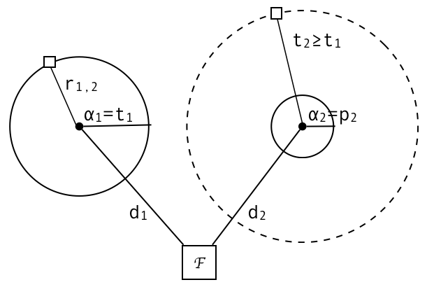
Figure 1: The ordering of the clients with respect to $t_{i}$ instead of $\alpha_{i}$.

Constraint (5), i.e. $r_{i,l}\leq t_{i}$ for $i<l$ follows, as client $i$ cannot be connected to a facility of distance larger than $t_{i}$. Moreover constraint (6) is valid, as otherwise solution $S^{\prime}$ which does not connect client $i$ to facility $\mathcal{F}$ would be cheaper.

Now we are left with justifying the opening cost constraints (1). Fix $l\in[k]$ and consider the moment just before $t_{l}$. We will count the contribution of each client towards opening $\mathcal{F}$. From Algorithm 1 the total contribution cannot exceed $f$. First, consider $i<l$. It is easy to see that if $i$ was already connected to some facility, then its offer is equal to $[r_{i,l}-d_{i}]^{+}$. Otherwise, as $t_{i}\leq t_{l}$, we know that $i$ already exhausted its potential, hence its offer is equal to $[p_{i}-d_{i}]^{+}$. Consider now $i\geq l$. From the description of Algorithm 1 and definition of $t_{i}$ its budget at this point is equal to $\min\{t_{i},p_{i}\}\geq\min\{t_{l},p_{i}\}$.

∎

Observe that $P(k)$ resembles the factor revealing program used in the analysis of the JMS algorithm for version without penalties [7]. However $P(k)$ has additional variables $p$ and minimas. Consider now the following program $\hat{P}(k,m)$

$$\max\hskip 5.0pt \frac{\sum_{i}{m_{i}t_{i}}-\lambda_{f}f}{\sum_{i}{m_{i}d_{i}}} (\hat{P}(k,m))$$

s.t.

$$\sum_{i=1}^{l-1}m_{i}\left[r_{i,l}-d_{i}\right]^{+}+\sum_{i=l}^{k}m_{i}\left[t_{l}-d_{i}\right]^{+}\leq f l\in[k]$$ (9)

$$(\ref{constraint:monotone}),(\ref{constraint:r-monotone}),(\ref{constraint:metric}),(\ref{constraint:nonneg1})$$

where $m$ is the vector of $m_{i}$’s. We claim that by losing arbitrarily small $\epsilon$, we can bound the value of $P(k)$ by the $\hat{P}(k,m)$ for some vector $m$ of natural numbers. This is captured by the following theorem, where $v(\textsc{sol},P)$ denotes the value of the solution sol to program $P$.

Theorem 2.2

For any $\epsilon>0$ and any feasible solution sol of value $v(\textsc{sol},P(k))$ to the program $P(k)$, there exists a vector $m$ of natural numbers and a feasible solution $\overline{\textsc{sol}}_{k,m}$ to program $\hat{P}(k,m)$ such that $v(\textsc{sol},P(k))\leq v(\overline{\textsc{sol}}_{k,m},\hat{P}(k,m))+\epsilon$.

Before we prove the above theorem, we show that it implies the desired bound on the approximation ratio. Note that the program $\hat{P}(k,m)$ is similar to the factor revealing program in the statement of Theorem 6.1 in [7] where their $k=\sum_{i=1}^{k}m_{i}$. The only difference is that it has additional constraints imposing that some clients are the same (we have $m_{i}$ copies of each client). However, this cannot increase the value of the program. Therefore, we obtain the same bi-factor approximation as the JMS algorithm [7].

Corollary 1

Algorithm 1 is a $(1.11,1.78)$-approximation algorithm for the ufl problem with penalties, i.e., it produces solutions whose cost can be bounded by $1.11$ times the optimal facility opening cost plus $1.78$ times the sum of the optimal connection cost and penalties.

We are left with the proof of Theorem 2.2 which we give in the subsection below.

2.2 Reducing the factor revealing programs

Proof (Proof of Theorem 2.2)

First, we give the overview of the proof and the intuition behind it. We have two main steps:

• Step 1 — Getting rid of $p$ and minimas
  We would like to get a rid of the variables $p_{i}$ and the minimas. To achieve this, we replace them with appropriate ratios $z_{i}$.

• Step 2 — Discretization
  We then make multiple copies of each client. For some of them, we assign penalty equal to its $t_{i}$ and for others — $d_{i}$. The portion of copies with positive penalty is equal to $z_{i}$.

For each step, we construct optimization programs and corresponding feasible solutions. The goal is to show, that in the resulting chain of feasible solutions and programs, the value of each solution can be upper-bounded by the value of the next solution. Formally, take any feasible solution $\textsc{sol}=(t^{*},d^{*},r^{*},p^{*},f^{*})$ to the program $P(k)$. In the following, we will construct solutions $\textsc{sol}_{1},\textsc{sol}_{2}$ and programs $P_{1}$ and $P_{2}$ such that $v(\textsc{sol},P(k))\leq v(\textsc{sol}_{1},P_{1})\leq v(\textsc{sol}_{2},P_{2})+\epsilon\leq v(\overline{\textsc{sol}}_{k,m},\hat{P}(k,m))+\epsilon$

Step 1 — getting rid of $p$ and minimas

Define $z^{*}_{i}=\frac{\min\{t^{*}_{i},p^{*}_{i}\}-d^{*}_{i}}{t^{*}_{i}-d^{*}_{i}}$ if $t^{*}_{i}-d^{*}_{i}>0$, and $z^{*}_{i}=0$ otherwise. Observe that $z^{*}_{i}\in[0,1]$ as $p^{*}_{i}\geq d^{*}_{i}$ by constraint (6). We claim that $\textsc{sol}_{1}=(t^{*},d^{*},r^{*},z^{*},f^{*})$ is a feasible solution to the following program $P_{1}(k)$

$$\max\hskip 5.0pt \frac{\sum_{i}{d_{i}+z_{i}(t_{i}-d_{i})}-\lambda_{f}f}{\sum_{i}{d_{i}}} (P_{1}(k))$$

s.t.

$$\sum_{i=1}^{l-1}z_{i}\left[r_{i,l}-d_{i}\right]^{+}+\sum_{i=l}^{k}z_{i}\left[t_{l}-d_{i}\right]^{+}\leq f l\in[k]$$ (10)

$$(\ref{constraint:monotone}),(\ref{constraint:r-monotone}),(\ref{constraint:metric}),(\ref{constraint:r-vs-t}),(\ref{constraint:nonneg1})$$

$$0\leq z_{i}\leq 1$$ (11)

and that the value of sol in $P(k)$ is the same as the value of $\textsc{sol}_{1}$ in $P_{1}(k)$. The latter property follows trivially as $\sum_{i}{d^{*}_{i}+z^{*}_{i}(t^{*}_{i}-d^{*}_{i})}=\sum_{i}{\min\{t^{*}_{i},p^{*}_{i}\}}$. To show feasibility, we have to argue that (10) is a valid constraint for $\textsc{sol}_{1}$. To this end we will use the following claim.

Claim

For any $x\leq t^{*}_{i}$, we have that

$$\left[\min\{x,p^{*}_{i}\}-d^{*}_{i}\right]^{+}\geq z^{*}_{i}\left[x-d^{*}_{i}\right]^{+}$$

Proof

Consider two cases:

1. $p^{*}_{i}\leq x$. In this case the left hand side is equal to $\left[p^{*}_{i}-d^{*}_{i}\right]^{+}$, while the right hand side is equal to $\frac{p^{*}_{i}-d^{*}_{i}}{t_{i}-d_{i}}\cdot\left[x-d^{*}_{i}\right]^{+}$. As $x\leq t^{*}_{i}$, the claim follows.

2. $p^{*}_{i}>x$. In this case the left hand side is equal to $\left[x-d^{*}_{i}\right]^{+}$, while the right hand side is equal to $z^{*}_{i}\cdot\left[x-d^{*}_{i}\right]^{+}$. As $z^{*}_{i}\leq 1$, the claim follows.

∎

Claim 2.2 together with the fact that $r^{*}_{i,l}\leq t^{*}_{i}$ for $i<l$ (constraint (5)) and $t^{*}_{l}\leq t^{*}_{i}$ for $l\leq i$ (constraint (2)) implies that

$$\sum_{i=1}^{l-1}\left[\min\{r^{*}_{i,l},p^{*}_{i}\}-d^{*}_{i}\right]^{+}+\sum_{i=l}^{k}\left[\min\{t^{*}_{l},p^{*}_{i}\}-d^{*}_{i}\right]^{+}\geq\sum_{i=1}^{l-1}z^{*}_{i}\left[r^{*}_{i,l}-d^{*}_{i}\right]^{+}+\sum_{i=l}^{k}z^{*}_{i}\left[t^{*}_{l}-d^{*}_{i}\right]^{+}$$

which shows feasibility of $\textsc{sol}_{1}$.

Step 2 — discretization

Take $M=N\cdot\lceil\max\limits_{i:z^{*}_{i}>0}{\frac{1}{z^{*}_{i}}}\rceil$, where $N=\lceil\frac{\lambda_{f}f^{*}}{\epsilon}\rceil$. Note that the value of $M$ depends on $\textsc{sol}_{1}$.

Define now program $P_{2}(k,M)$, by adding to the program $P_{1}(k)$ the constraints $z_{i}\in\{0,\frac{1}{M},\frac{2}{M},\dots,\frac{M}{M}\}$ for each $i$. We construct a solution to this program in the following way. Take $z^{\prime}_{i}=\frac{\lceil z^{*}_{i}\cdot M\rceil}{M}$ and $f^{\prime}=\frac{N+1}{N}f^{*}$. Let now $\textsc{sol}_{2}=(t^{*},d^{*},r^{*},z^{\prime},f^{\prime})$.

First, we claim that $\textsc{sol}_{2}$ is feasible to program $P_{2}(k,M)$. To see this, observe that $z^{*}_{i}\leq z^{\prime}_{i}\leq\frac{N+1}{N}z^{*}_{i}$ and $z^{\prime}\in\{0,\frac{1}{M},\frac{2}{M},\dots,\frac{M}{M}\}$. The feasibility follows from multiplying both sides of the constraint (10) by $\frac{N+1}{N}$.

Second, we claim that $v(\textsc{sol}_{1},P_{1}(k))\leq v(\textsc{sol}_{2},P_{2}(k,M))+\epsilon$. We have the following:

$$v(\textsc{sol}_{1},P_{1}(k)) =\frac{\sum_{i}{d^{*}_{i}+z^{*}_{i}(t^{*}_{i}-d^{*}_{i})}-\lambda_{f}f^{*}}{\sum_{i}{d^{*}_{i}}}$$

$$\leq\frac{\sum_{i}{d^{*}_{i}+z^{\prime}_{i}(t^{*}_{i}-d^{*}_{i})}-\frac{N+1}{N}\lambda_{f}f^{*}+\frac{1}{N}\lambda_{f}f^{*}}{\sum_{i}{d^{*}_{i}}}$$

$$\leq\frac{\sum_{i}{d^{*}_{i}+z^{\prime}_{i}(t^{*}_{i}-d^{*}_{i})}-\lambda_{f}f^{\prime}+\epsilon}{\sum_{i}{d^{*}_{i}}}$$

$$\leq v(\textsc{sol}_{2},P_{2}(k,M))+\epsilon$$

where in the last line we use the fact that for the normalization, the denominator $\sum_{i}{d_{i}}$ can be fixed to be equal 1.

Finishing the proof

Define now $m_{i}=M\cdot z^{\prime}_{i}$ and consider program $\hat{P}(k,m)$. Note, that all the $m_{i}$ variables are natural numbers as required. It remains to construct the solution $\overline{\textsc{sol}}_{k,m}$ for $\hat{P}(k,m)$. Let $\hat{f}=M\cdot f^{\prime}$ and $\overline{\textsc{sol}}_{k,m}=(t^{*},d^{*},r^{*},\hat{f})$. To see that the constraint (9) is satisfied, multiply by $M$ both sides of valid constraint (10) for $\textsc{sol}_{2}$ (i.e. $\sum_{i=1}^{l-1}z^{\prime}_{i}\left[r^{*}_{i,l}-d^{*}_{i}\right]^{+}+\sum_{i=l}^{k}z^{\prime}_{i}\left[t^{*}_{l}-d^{*}_{i}\right]^{+}\leq f^{\prime}$).

It remains to bound the value of $\textsc{sol}_{2}$ with the value of $\overline{\textsc{sol}}_{k,m}$:

$$v(\textsc{sol}_{2},P_{2}(k,m)) =\frac{\sum_{i}{d^{*}_{i}+z^{\prime}_{i}(t^{*}_{i}-d^{*}_{i})}-\lambda_{f}f^{\prime}}{\sum_{i}{d^{*}_{i}}}$$

$$=\frac{\sum_{i}{d^{*}_{i}M+z^{\prime}_{i}M(t^{*}_{i}-d^{*}_{i})}-\lambda_{f}Mf^{\prime}}{\sum_{i}{Md^{*}_{i}}}$$

$$=\frac{\sum_{i}{d^{*}_{i}M+m_{i}(t^{*}_{i}-d^{*}_{i})}-\lambda_{f}Mf^{\prime}}{\sum_{i}{Md^{*}_{i}}}$$

$$=\frac{\sum_{i}{m_{i}t^{*}_{i}}-\lambda_{f}Mf^{\prime}+\sum_{i}{(M-m_{i})d^{*}_{i}}}{\sum_{i}{m_{i}d^{*}_{i}}+\sum_{i}{(M-m_{i})d^{*}_{i}}}$$

$$\leq\frac{\sum_{i}{m_{i}t^{*}_{i}}-\lambda_{f}Mf^{\prime}}{\sum_{i}{m_{i}d^{*}_{i}}}$$

$$=v(\overline{\textsc{sol}}_{k,m},\hat{P}(k,m))$$

where the last inequality follows from the fact that the nominator is larger than the denominator (as this fraction gives an upper bound on approximation factor which must be greater than 1). ∎

3 Combining algorithms for FLP

By Corollary 1, the adapted JMS algorithm is a $(1.11,1.78)$-approximation algorithm for the ufl problem with penalties.

It remains to note that the applicability of the LP-rounding algorithms for ufl to the flp problem has already been studied. In particular the algorithm 4.2 of [11] is an adaptation of the LP rounding algorithms for ufl by Byrka and Aardal [1] and Li [10] to the setting with penalties.

Note also that Qiu and Kern [14] made an attempt on finalising the work on ufl with penalties and analysing the adapted JMS algorithm, and correctly argued that once the analogue of the JMS algorithm for the penalty version of the problem is known the improved approximation ratio for the variant with penalties will follow. Their analysis of the adapted JMS was incorrect (and the paper withdrawn from arxiv). By providing the missing analysis of the adapted JMS, we fill in the gap and obtain:

Corollary 2

There exists a $1.488$-approximation algorithm for the flp.

Corollary 3

For any $\lambda_{f}\geq 1.6774$ and $\lambda_{c+p}=1+\frac{2}{e^{\lambda_{f}}}$ there exists a bifactor $(\lambda_{f},\lambda_{c+p})$-approximation algorithm for flp.

4 Solving NCC-FL with algorithms for FLP

We will now discuss how to use algorithms for the flp problem to solve ncc-fl problem. To this end we introduce yet another variant of the problem: facility location with penalties and multiplicities flpm. In this setting each client $j$ has two additional parameters: penalty $p_{j}$ and multiplicity $m_{j}$, both being nonnegative real numbers. If client $j$ is served by facility $i$ the service cost is $m_{j}\cdot d_{ij}$ and if it is not served by any facility the penalty cost is $m_{j}\cdot p_{j}$.

Lemma 1

There is an approximation preserving reduction from ncc-fl to flpm.

Proof

Take an instance $I=(F,D,d,g)$ of the ncc-fl problem with $|F|=n$ facilities. Create the instance $I^{\prime}=(F,D^{\prime},d^{\prime},p,m)$ as follows. The set of the facilities is the same as in original instance. For each client $j\in D$, we will create in $I^{\prime}$ multiple copies of $j$.

Fix a single client $j$. Sort all the facilities by their distance to $j$ and let $d^{(j)}_{1}\leq d^{(j)}_{2}\leq\dots\leq d^{(j)}_{n}$ be the sorted distances. For every $k\in[n-1]$ define also

$$m^{(j)}_{k}=\frac{g_{j}(d^{(j)}_{k})-g_{j}(d^{(j)}_{k-1})}{d^{(j)}_{k}-d^{(j)}_{k-1}}-\frac{g_{j}(d^{(j)}_{k+1})-g_{j}(d^{(j)}_{k})}{d^{(j)}_{k+1}-d^{(j)}_{k}}$$ (12)

where for convenience we define $d^{j}_{0}=g_{j}(d^{(j)}_{0})=0$. Let also

$$m^{(j)}_{n}=\frac{g_{j}(d^{(j)}_{n})-g_{j}(d^{(j)}_{n-1})}{d^{(j)}_{n}-d^{(j)}_{n-1}}$$ (13)

Observe that concavity of $g_{j}$ implies that every $m^{(j)}_{k}$ is nonnegative. Now, for each $k\in[n]$, we create a client $j_{k}$ in the location of $j$ with penalty set to $p_{j_{k}}=d^{(j)}_{k}$ and multiplicity $m^{(j)}_{k}$. It remains to show that for any subset of facilities $F^{\prime}\subseteq F$ it holds that $cost_{I}(F^{\prime})=cost_{I^{\prime}}(F^{\prime})$, where $cost_{.}(F^{\prime})$ denotes the cost of a solution obtained by optimally assigning clients to facilities in $F^{\prime}$. To see this, consider a client $j\in D$ and its closest facility $f$ in $F^{\prime}$. Let $k$ be the index of $f$ in the vector $d^{(j)}$ of sorted distances, i.e. the distance between $j$ and $f$ is $d^{(j)}_{k}$. Observe that for the solution $F^{\prime}$ in $I^{\prime}$ the clients $j_{1},\dots,j_{i},\dots,j_{k-1}$ pay their penalty $d^{(j)}_{i}$ (as the penalty is at most the distance to the closest facility) and the clients $j_{k},\dots j_{n}$ can be connected to $f$. Therefore, we require that for any $k$,

$$g_{j}(d^{(j)}_{k})=\sum_{i=1}^{k-1}m^{(j)}_{i}d^{(j)}_{i}+\sum_{i=k}^{n}m^{(j)}_{i}d^{(j)}_{k}$$ (14)

It can be observed, that $m^{(j)}_{i}$ as defined in (12) and (13) satisfy the system of equalities (14). ∎

It remains to show how to solve flpm. Recall that our algorithm for flp is a combination of the JMS algorithm and an LP rounding algorithm. We will now briefly argue that each of the two can be adapted to the case with multiplicities.

To adapt the JMS algorithm, one needs to take multiplicities into account when calculating the contributions of individual clients towards facility opening. Then in the analysis multiplicities can be scaled up and discretized to lose only an epsilon factor. Here we utilize that non-polynomial blowup in the number of clients is not a problem in the analysis.

To adapt the LP rounding algorithm, we first observe that multiplicities can easily be introduced to the LP formulation, and hence solving an LP relaxation of the problem with multiplicities is not a problem. Next, we utilize that the analysis of the expected connection (and penalty) cost of the algorithm is a per-client analysis. Therefore, by the linearity of expectation combined with linearity of the objective function with respect to multiplicities, the original analysis applies to the setting with multiplicities. A similar argument was previously utilized in [2].

5 Approximation algorithms for SIRPFL

In this section we give the improved algorithms for all the three variants of the Star Inventory Routing Problem with Facility Location that was recently introduced by Jiao and Ravi [9]. First, we recall the definition. We are given the set of facilities $F$ and clients $D$ in the metric space ($d$), a time horizon $1,\dots,T$, a set of demand points $(j,t)$ with $u^{j}_{t}$ units of demand requested by client $j$ due by day $t$, facility opening costs $f_{i}$, holding costs $h^{j}_{s,t}$ per unit of demand delivered on day $s$ serving ($j,t$). The objective is to open a set of facilities and plan the deliveries to each client to minimize the total facility opening costs, client-facility connections and storage costs. Consider first the uncapacitated variant in which every delivery can contain unbounded number of goods.

Observe that once the decision which facilities to open is made, each client can choose the closest open facility and use it for all the deliveries. In that case, we would be left with a single-item lot-sizing problem which can be solved to optimality. The above view is crucial for our approach. Observe that we can precompute all the single-item lot-sizing instances for every pair $(i,j)$. Now we are left with a specific facility location instance that is captured by ncc-fl. The following lemma proves this reduction.

Lemma 2

There is a 1.488 approximation algorithm for uncapacitated sirpfl.

Proof (Proof of Lemma 2)

For each $j\in D$ and $i\in F$ solve the instance of a single-item lot-sizing problem with delivery cost $d_{j,i}$ and demands and holding costs for client $j$ to optimality [17]. Now define $g_{j}(d_{j,i})$ to be the cost of this computed solution and linearly interpolate other values of function $g$.

It is now easy to see that $g_{j}$ is an increasing concave function. This follows from the fact, that the optimum solution to the lot-sizing problem with delivery cost $x$ is also a feasible solution to the problem with delivery cost $\alpha\cdot x$ for $\alpha\geq 1$. Moreover the value of this solution for increased delivery cost is at most $\alpha$ times larger.

In this way we obtained the instance of ncc-fl problem which can be solved using the algorithm of Lemma 1. Once we know which facilities to open, we use optimal delivery schedules computed at the beginning. ∎

Jiao and Ravi studied also capacitated splittable and capacitated unsplittable variants obtaining $24$ and $48$ approximation respectively [9]. By using corresponding $3$ and $6$ approximation for the capacitated splittable and unsplittable Inventory Access Problem (IAP) given in [9] (the variants of single-item lot-sizing) and a similar reduction to ncc-fl as above while using a suitable bi-factor algorithm for FLP we are able to give improved approximation algorithms for both capacitated variants of sirpfl.

Lemma 3

There is a $3.236$-approximation algorithm for capacitated splittable sirpfl and $6.029$-approximation algorithm for capacitated unsplittable sirpfl.

Proof (Proof of Lemma 3)

The approach is the same as in proof of Lemma 2 but with a little twist. We give details only for splittable case as the unsplittable variant follows in the same way.

For each $j\in D$ and $i\in F$ run the $3$-approximation algorithm [9] for the instance of a corresponding splittable Inventory Access Problem problem with delivery cost $d_{j,i}$ and demands and holding costs for client $j$.

Notice that we cannot directly define $g_{j}(d_{j,i})$ to be the cost of the computed solution as the resulting function would not necessarily be concave (due to using approximate solutions instead of optimal).

Therefore, we construct $g_{j}$ for each $j\in D$ in a slightly different way. W.l.o.g assume that $d_{j,1}\leq d_{j,2}\dots\leq d_{j,n}$. Let also $A(x)$ be the computed $3$-approximate solution for IAP with delivery cost $x$ and let $V(S,x)$ be the value of solution $S$ for IAP with delivery cost $x$. Notice that for $x<y$, the solution $A(x)$ is feasible for the same IAP instance but with delivery cost $y$. In particular, the following bound on cost is true: $V(A(x),y)\leq\frac{y}{x}\cdot V(A(x),x)$.

We now construct a sequence of solutions. Let $S_{1}=A(d_{j,1})$. Now, for each $i\in[n-1]$ define:

$$S_{i+1}=\begin{cases}S_{i},&\text{if }V(S_{i},d_{j,i+1})<V(A(d_{j,i+1}),d_{j,i+1})\\ A(d_{j,i+1}),&\text{otherwise}\end{cases}$$

Finally take $g(d_{j,i})=V(S_{i},d_{j,i})$ and linearly interpolate other values. It can be easily observed that $g_{j}$ is a nondecreasing concave function.

Finally, we are using the bifactor ($\lambda_{f},1+2e^{-\lambda_{f}}$)-approximation algorithm to solve the resulting instance of ncc-fl. Because we also lose a factor of $3$ for connection cost, the resulting ratio is equal to $\max\{\lambda_{f},3\cdot(1+2e^{-\lambda_{f}})\}$. The two values are equal for $\lambda_{f}\approx 3.23594$. ∎

References

- [1] Byrka, J., Aardal, K.: An optimal bifactor approximation algorithm for the metric uncapacitated facility location problem. SIAM Journal on Computing 39(6), 2212–2231 (2010)
- [2] Byrka, J., Skowron, P., Sornat, K.: Proportional approval voting, harmonic k-median, and negative association. In: 45th International Colloquium on Automata, Languages, and Programming (ICALP 2018). Schloss Dagstuhl-Leibniz-Zentrum fuer Informatik (2018)
- [3] Charikar, M., Khuller, S., Mount, D.M., Narasimhan, G.: Algorithms for facility location problems with outliers. In: Proceedings of the Twelfth Annual Symposium on Discrete Algorithms, January 7-9, 2001, Washington, DC, USA. pp. 642–651 (2001)
- [4] Chudak, F.A., Shmoys, D.B.: Improved approximation algorithms for the uncapacitated facility location problem. SIAM J. Comput. 33(1), 1–25 (2003)
- [5] Geunes, J., Levi, R., Romeijn, H.E., Shmoys, D.B.: Approximation algorithms for supply chain planning and logistics problems with market choice. Math. Program. 130(1), 85–106 (2011)
- [6] Guha, S., Khuller, S.: Greedy strikes back: Improved facility location algorithms. Journal of Algorithms 31(1), 228 – 248 (1999)
- [7] Jain, K., Mahdian, M., Markakis, E., Saberi, A., Vazirani, V.V.: Greedy facility location algorithms analyzed using dual fitting with factor-revealing lp. J. ACM 50(6), 795–824 (Nov 2003)
- [8] Jain, K., Vazirani, V.V.: Approximation algorithms for metric facility location and k-median problems using the primal-dual schema and lagrangian relaxation. J. ACM 48(2), 274–296 (2001)
- [9] Jiao, Y., Ravi, R.: Inventory routing problem with facility location. In: Friggstad, Z., Sack, J.R., Salavatipour, M.R. (eds.) Algorithms and Data Structures. pp. 452–465. Springer International Publishing, Cham (2019)
- [10] Li, S.: A 1.488 approximation algorithm for the uncapacitated facility location problem. In: International Colloquium on Automata, Languages, and Programming. pp. 77–88. Springer (2011)
- [11] Li, Y., Du, D., Xiu, N., Xu, D.: Improved approximation algorithms for the facility location problems with linear/submodular penalties. Algorithmica 73(2), 460–482 (2015)
- [12] Mahdian, M., Ye, Y., Zhang, J.: Improved approximation algorithms for metric facility location problems. In: Approximation Algorithms for Combinatorial Optimization, 5th International Workshop, APPROX 2002, Rome, Italy, September 17-21, 2002, Proceedings. pp. 229–242 (2002)
- [13] Nagarajan, V., Shi, C.: Approximation algorithms for inventory problems with submodular or routing costs. Mathematical Programming 160(1-2), 225–244 (2016)
- [14] Qiu, X., Kern, W.: On the factor revealing lp approach for facility location with penalties. arXiv preprint arXiv:1602.00192 (2016)
- [15] Sviridenko, M.: Personal communication. Cited in S. Guha, Approximation algorithms for facility location problems, PhD thesis, Stanford, 2000
- [16] Sviridenko, M.: An improved approximation algorithm for the metric uncapacitated facility location problem. In: Integer Programming and Combinatorial Optimization, 9th International IPCO Conference, Cambridge, MA, USA, May 27-29, 2002, Proceedings. pp. 240–257 (2002)
- [17] Wagner, H.M., Whitin, T.M.: Dynamic version of the economic lot size model. Management science 5(1), 89–96 (1958)
- [18] Xu, G., Xu, J.: An LP rounding algorithm for approximating uncapacitated facility location problem with penalties. Inf. Process. Lett. 94(3), 119–123 (2005)
- [19] Xu, G., Xu, J.: An improved approximation algorithm for uncapacitated facility location problem with penalties. J. Comb. Optim. 17(4), 424–436 (2009)