Improving Non-Intrusive Load Disaggregation through an Attention-Based Deep Neural Network

Abstract

Energy disaggregation, known in the literature as Non-Intrusive Load Monitoring (NILM), is the task of inferring the power demand of the individual appliances given the aggregate power demand recorded by a single smart meter which monitors multiple appliances. In this paper, we propose a deep neural network that combines a regression subnetwork with a classification subnetwork for solving the NILM problem. Specifically, we improve the generalization capability of the overall architecture by including an encoder–decoder with a tailored attention mechanism in the regression subnetwork. The attention mechanism is inspired by the temporal attention that has been successfully applied in neural machine translation, text summarization, and speech recognition. The experiments conducted on two publicly available datasets—REDD and UK-DALE—show that our proposed deep neural network outperforms the state-of-the-art in all the considered experimental conditions. We also show that modeling attention translates into the network’s ability to correctly detect the turning on or off an appliance and to locate signal sections with high power consumption, which are of extreme interest in the field of energy disaggregation.

I Introduction

Non-Intrusive Load Monitoring (NILM) is the task of estimating the power demand of each appliance given aggregate power demand signal recorded by a single electric meter monitoring multiple appliances [1]. In the last years, machine learning and optimization played a significant role in the research on NILM [2, 3]. In the literature, solutions based on k-Nearest Neighbor (k-NN), Support Vector Machine (SVM), Matrix Factorization have been proposed [4, 5]. A practical approach to NILM has to handle real power measurements sampled at intervals of seconds or minutes. In this setting, one of the most popular approaches is based on the Hidden Markov Model (HMM) [6], because of its ability to model transitions in consumption levels of real energy consumption for target appliances. Some successive papers focused on enhancing the expressive power of this class of methods [7, 8]. Recently, the energy disaggregation problem has been reformulated as a multi-label classification problem [9]. In order to detect the active appliances at each time step, the idea is to associate each value of the main power to a vector of labels of length equal to the number of appliances, that are set to 1 if the appliance is active and 0 otherwise. The reformulated problem has been solved with different approaches [10, 11, 12]. However, there is no direct way to derive the power consumption for each appliance at that time step. During the last years, approaches based on deep learning have received particular attention as they exhibited noteworthy disaggregation performance. Deep Neural Networks (DNNs) have been successfully applied for the first time to NILM by Kelly and Knottenbelt in [13], who coined the term “Neural NILM”. Neural NILM is a nonlinear regression problem that consists of training a neural network for each appliance in order to predict a time window of the appliance load given the corresponding time window of aggregated data. Kelly and Knottenbelt proposed three different neural networks to perform NILM with high-frequency time series data: a recurrent neural network (RNN) using Long Short-Term Memory units (LSTM); a Denoising Autoencoder (DAE); and a regression model that predicts the start time, end time, and average power demand of each appliance. The capability of LSTMs to successfully learn long-range temporal dependencies of time series data makes it a suitable candidate for NILM. Their first approach is based on stacked layers of LSTM units combined with a Convolutional Neural Network (CNN) at the beginning of the network to automatically extract features from the raw data. In the same paper, NILM is treated as a noise reduction problem, in which the disaggregated load represents the clean signal, and the aggregated signal is considered corrupted by the presence of the remaining appliances and by the measurement noise. For this purpose, noise reduction is performed by means of a DAE composed of convolutional layers and fully connected layers. In the experiments conducted by the authors, the DAE network outperforms the LSTM-based architecture and the other approaches frequently employed for this problem, such as HMMs and Combinatorial Optimization. In [14], an empirical investigation of deep learning methods is conducted by using two types of neural network architectures for NILM. The first neural network solves a regression problem which estimates the transient power demand of a single appliance given the whole series of the aggregate power. The second type of network is a multi-layer RNN using LSTM units, which is similar to the structure used in [13]. Zhang et al. [15] proposed instead a sequence-to-point learning for energy disaggregation where the midpoint of an appliance window is treated as classification output of a neural network with the aggregate window being the input. Bonfigli et al. [16] proposed different algorithmic and architecture improvements to the DAE for NILM, showing that the Neural NILM approach improves on the best known NILM approaches not based on DNNs like Additive Factorial Approximate Maximum A Posteriori estimation (AFAMAP) by Kolter and Jaakkola [6]. Compared to the work in [13], their DAE approach is improved by introducing pooling and upsampling layers in the architecture and a median filter in the disaggregation phase to reconstruct the output signal from the overlapped portions of the disaggregated signal. Shin et al. [17] proposed a subtask gated network (SGN) that combines two CNNs, namely, a regression subnetwork and a classification subnetwork. The building block of the two subnetworks is the sequence-to-sequence CNN proposed in [15]. In their work, the regression subnetwork is used to infer the initial power consumption, whereas the classification subnetwork focuses on the binary classification of the appliance state (on/off). The final estimate of the power consumption is obtained by multiplying the regression output with the probability classification output. In the experiments conducted by the authors, the SGN outperforms HHMs and state-of-the-art CNN architectures that have been proposed recently [13, 15]. Chen et al. [18] adopted the structure of the SGN proposed in [17] and added to the SGN backbone a Generative Adversarial Network (GAN). In their model, the disaggregator for a given appliance is followed by a generator that produces the load pattern for that appliance. They show that adding the adversarial loss can help the model to produce more accurate result with respect to the basic SGN architecture. None of these state-of-the art deep learning models use RNNs. In fact, in the NILM literature, CNNs have always shown better performance than RNNs, even though RNNs are still widely employed for sequence modeling tasks. In [19], a CNN-based DNN has been combined with data augmentation and an effective postprocessing phase, improving its ability to correctly detect the activation of each appliance with a small amount of data available. The attention mechanism applied to NILM is a relatively new idea [20]. The DNN in [20] remarkably improves over Kelly’s DAE when trained and tested on the same house. On the other hand, the generalization capability on houses not seen during the training is modest. Moreover, training and testing for the NILM task are time-consuming as they used the same architecture proposed in [21] for machine translation which consists of RNN layers in both the encoder and the decoder.

In this paper, we propose a RNN-based encoder–decoder model to extract appliance specific power usage from the aggregated signal and we enhance it with a scalable and lightweight attention mechanism designed for the energy disaggregation task. More in detail, we substantially improve the generalization capability of the SGN by Shin et al. by encapsulating our model in the regression subnetwork and by combining it with the classification subnetwork. The implemented attention mechanism has the function to strengthen the representational power of the neural network to locate the positions of the input sequence where the relevant information is present. The intuition is that our attention-based model could help the energy disaggregation task by assigning importance to each position of the aggregated signal which corresponds to the position of a state change of the target appliance. This feature is crucial for developing appliance models that generalize well on buildings not seen during the training.

The proposed DNN is tested on two publicly available datasets—REDD and UK-DALE—and the performance is evaluated using different metrics. The obtained results show that our algorithm outperforms state-of-the-art DNNs in all the addressed experimental conditions. The paper is organized as follows. Section II describes the NILM problem. Section III presents our DNN architecture. Section IV describes the experimental procedure and the obtained results. Finally, Section V concludes the paper.

II NILM Problem

Given the aggregate power consumption $(x_{1},\dots,x_{T})$ from $N$ active appliances at the entry point of the meter, the task of the NILM algorithm is to deduce the contribution $(y_{1}^{i},\dots,y_{T}^{i})$ of appliance $i=1,\dots,N$, such that at time $t=1,\dots,T$, the aggregate power consumption is given by the sum of the power consumption of all the known appliances plus a noise term. The energy disaggregation problem can be stated as

$$x_{t}=\sum_{i=1}^{N}y_{t}^{i}+\epsilon_{t},$$ (1)

where $x_{t}$ is the aggregated active power measured at time $t$, $y_{t}^{i}$ is the individual contribution of appliance $i$, $N$ is the number of appliances, and $\epsilon_{t}$ is a noise term. In a denoised scenario, there is no noise term, whereas in a noised scenario, $\epsilon_{t}$ is given by the total contribution from appliances not included and the measurement noise. Similarly to the work in [13], we refer to the power over a complete cycle of an appliance as an appliance activation.

III Encoder–Decoder with Attention Mechanism

In this section, we describe the adopted attention mechanism and DNN architecture for solving the NILM problem.

III-A Attention Mechanism

In the classical setting, a sequence-to-sequence network is a model consisting of two components called the encoder and decoder [22]. The encoder is an RNN that takes an input sequence of vectors $(x_{1},\dots,x_{T})$, where $T$ is the length of input sequence, and encodes the information into fixed length vectors $(h_{1},\dots,h_{T})$. This representation is expected to be a good summary of the entire input sequence. The decoder is also an RNN which is initialized with a single context vector $c=h_{T}$ as its inputs and generates an output sequence $(y_{1},\dots,y_{N})$ vector by vector, where $N$ is the length of output sequence. At each time step, $h_{t}$ and $\sigma_{t}$ denote the hidden states of the encoder and decoder, respectively. There are two well-known challenges with this traditional encoder–decoder framework. First, a critical disadvantage of single context vector design is the incapability of the system to remember long sequences: all the intermediate states of the encoder are eliminated and only the final hidden state vector is used to initialize the decoder. This technique works only for small sequences, however, as the length of the sequence increases, the vector becomes a bottleneck and may lead to loss of information [23]. Second, it is unable to capture the need of alignment between input and output sequences, which is an essential aspect of structured output tasks such as machine translation or text summarization [24]. The attention mechanism, first introduced for machine translation by Bahdanau et al. [21], was born to address these problems. The novelty in their approach is the introduction of an alignment function that finds for each output word significant input words. In this way, the neural network learns to align and translate at the same time. The central idea behind the attention is not to discard the intermediate encoder states but to combine and utilize all the states in order to construct the context vectors required by the decoder to generate the output sequence. This mechanism induces attention weights over the input sequence to prioritize the set of positions where relevant information is present. Following the definition from Bahdanau et al., attention-based models compute a context vector $c_{t}$ for each time step as the weighted sum of all hidden states of the encoder. Their corresponding attention weights are calculated as

$$\footnotesize e_{tj}=f(\sigma_{t-1},h_{j}),\quad\alpha_{tj}=\frac{exp(e_{tj})}{\sum_{k=1}^{T}exp(e_{tk})},\quad c_{t}=\sum_{j=1}^{T}\alpha_{tj}h_{j},$$ (2)

where $f$ is a learned function that computes a scalar importance value for $h_{j}$ given the value of $h_{j}$ and the previous state $\sigma_{t-1}$ and each attention weight $\alpha_{tj}$ determines the normalized importance score for $h_{j}$. As shown in Figure 1, the context vectors $c_{t}$ are then used to compute the decoder hidden state sequence, where $\sigma_{t}$ depends on $\sigma_{t-1}$, $c_{t}$, and $y_{t-1}$. The attention weights can be learned by incorporating an additional feed-forward neural network that is jointly trained with encoder–decoder components of the architecture.

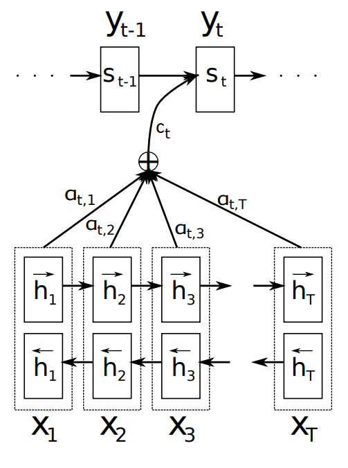
Figure 1: Original graphical representation of the attention model by Bahdanau et al. in [21].

The intuition is that an attention-based model could help in the energy disaggregation task by assigning importance to each position of the aggregated signal which corresponds to the position of an activation, or more generally, to a state change of the target appliance. This allows the neural network to focus its representational power on selected time steps of the target appliance in the aggregated signal, rather than on the activations of non-target appliances, hopefully yielding more accurate predictions. In fact, some events (e.g., turning on or off an appliance) or signal sections (e.g., high power consumption) are more important than other parts within the input signal. For this reason, being able to correctly detect the corresponding time steps can play a key role in the disaggregation task. In neural machine translation, languages are typically not aligned because of the word ordering between the source and the target language. For the NILM problem, the aggregated power consumption is perfectly aligned with the load of the corresponding appliance and the alignment is known ahead of time. For this reason, to amplify the contribution of an appliance activation in the aggregated signal, we use a simplified attention model inspired by Raffel and Ellis [25], that combines all the hidden states of the encoder using their relative importance. The attention mechanism can be formulated as

$$e_{t}=a(h_{t}),\quad\alpha_{t}=\frac{exp(e_{t})}{\sum_{j=1}^{T}exp(e_{j})},\quad c=\sum_{t=1}^{T}\alpha_{t}h_{t},$$ (3)

where $a$ is a learnable function the depends only on the hidden state vector of the encoder $h_{t}$. The function $a$ can be implemented with a feed-forward network that learns a particular attention weight $\alpha_{t}$ that determines the normalized importance score for $h_{j}$. This allows the network to recognize the time steps that are more important to the desired output as the ones having higher attention value.

III-B Model Design

From a practical point of view, DNNs use partial sequences obtained with a sliding window technique. The duration of an appliance activation is used to determine the size of the window that selects the input and output sequences for the NILM modeling. To be precise, let $\boldsymbol{x_{t,L}}=(x_{t},\dots,x_{t+L-1})$ and $\boldsymbol{y_{t,L}^{i}}=(y_{t}^{i},\dots y_{t+L-1}^{i})$ be, respectively, the partial aggregate and appliance sequences of length $L$ starting at time $t$. In addition, we build the auxiliary state sequence $(s_{1}^{i},\dots,s_{T}^{i})$, where $s_{t}^{i}\in\{0,1\}$ represent the on/off state of the appliance $i$ at time $t$. The state of an appliance is considered “on” when the consumption is greater than some threshold and “off” when the consumption is less or equal the same threshold. We use the notation $\boldsymbol{s_{t,L}^{i}}=(s_{t},\dots,s_{t+L-1})$ for the partial state sequences of length $L$ starting at time $t$. Our idea is to exploit the structure of the SGN architecture proposed in [17] as the building block of the model. This general framework uses an auxiliary sequence-to-sequence classification subnetwork that is jointly trained with a standard sequence-to-sequence regression subnetwork. The difference here is that we generate a more accurate estimate of the power consumption by performing the regression subtask with a scalable RNN-based encoder–decoder with attention mechanism. The intuition behind the proposed model is that the tailored attention mechanism allows the regression subnetwork to implicitly detect and assign more importance to some events (e.g., turning on or off of the appliance) and to specific signal sections (e.g., high power consumption), whereas the classification subnetwork helps the disaggregation process by enforcing explicitly the on/off states.

Differently from the DNN in [20], the scalability of the overall architecture is ensured by the regression subnetwork where no RNN is needed in the decoder. In fact, the adopted attention mechanism allows one to decouple the input representation from the output and the structure of the encoder from the structure of the decoder. We exploit these benefits and we design a hybrid encoder–decoder which is based on a combination of convolutional layers and recurrent layers for the encoder and fully connected layers for the decoder.

III-C Network Topology

Let $f_{reg}^{i}\colon\mathbb{R}_{+}^{L}\to\mathbb{R}_{+}^{L}$ be the appliance power estimation model, then the regression subnetwork learns the mapping $\boldsymbol{\hat{p}_{t,L}^{i}}=f_{reg}^{i}(\boldsymbol{x_{t,L}})$. The topology of the regression subnetwork is as follows.

Encoder: The encoder network is composed by a CNN with 4 one-dimensional convolutional layers (Conv1D) with ReLU activation function that processes the input aggregated signal and extracts the appliance-specific signature as a set of feature maps. Finally, a RNN takes as input the set of feature maps and produces the sequence of the hidden states summarizing all the information of the aggregated signal. We use Bidirectional LSTM (BiLSTM) in order to get the hidden states $h_{t}$ that summarize the information from both directions. A bidirectional LSTM is made up of a forward LSTM $\overrightarrow{g}$ that reads the sequence from left to right and a backward LSTM $\overleftarrow{g}$ that reads it from right to left. The final sequence of the hidden states of the encoder is obtained by concatenating the hidden state vectors from both directions, i.e., $h_{t}=[\overrightarrow{h_{t}};\overleftarrow{h_{t}}]^{T}$.

Attention: The attention unit between the encoder and the decoder consists of a single layer feed-forward neural network that computes the attention weights and returns the context vector as a weighted average of the output of the encoder over time. Not all the feature maps produced by the CNN have equal contribution in the identification of the activation of the target appliance. Thus, the attention mechanism captures salient activations of the appliance, extracting more valuable feature maps than others for the disaggregation. The implemented attention unit is shown in Figure 2, and it is mathematically defined as

$$e_{t}=V_{a}^{T}tanh(W_{a}h_{t}+b_{a}),$$ (4)

$$\alpha_{t}=softmax(e_{t}),$$ (5)

$$c=\sum_{t=1}^{T}\alpha_{t}h_{t},$$ (6)

where $V_{a}$, $W_{a}$, and $b_{a}$ are the attentions parameters jointly learned with the other components of the architecture. The output of the attention unit is the context vector $c$ that is used as the input vector for the following decoder.

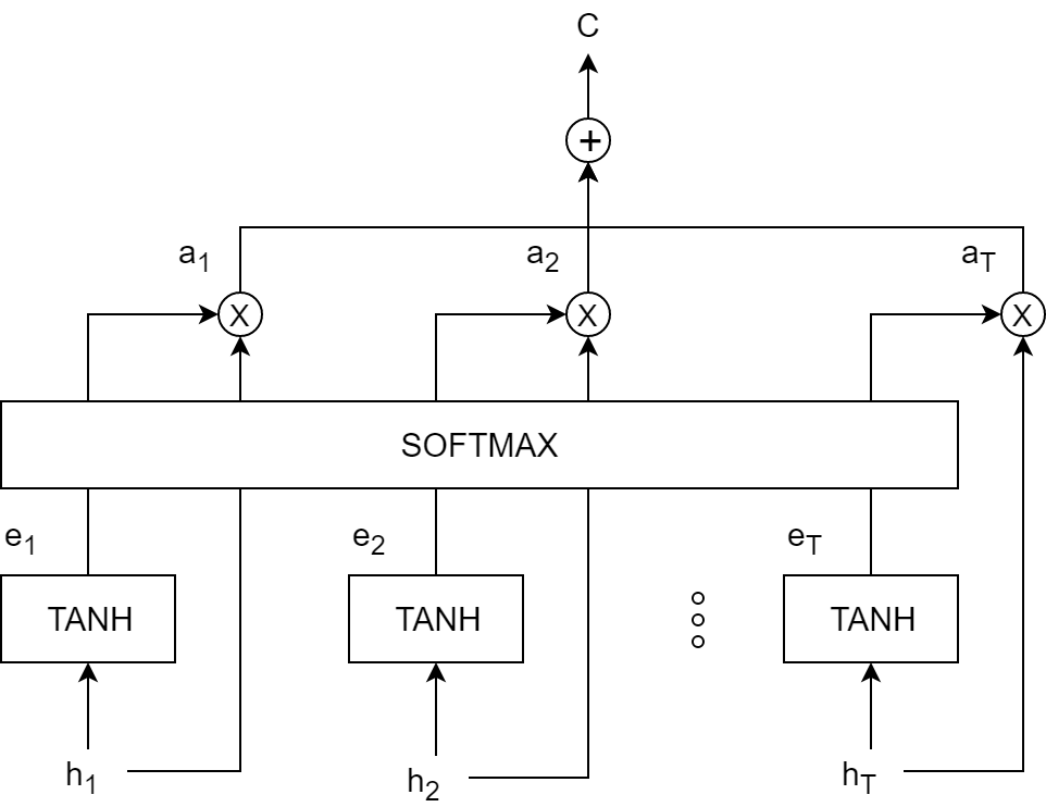
Figure 2: Graphical illustration of the implemented attention unit.

Decoder: The decoder network is composed by 2 fully connected layers (Dense). The second layer has the same number of units of the sequence length $L$.

The exact configuration of regression subnetwork is as follows:

1. Input (sequence length $L$ determined by the appliance duration)

2. Conv1D (convolutional layer with $F$ filters, kernel size $K$, stride $1$, and ReLU activation function)

3. Conv1D (convolutional layer with $F$ filters, kernel size $K$, stride $1$, and ReLU activation function)

4. Conv1D (convolutional layer with $F$ filters, kernel size $K$, stride $1$, and ReLU activation function)

5. Conv1D (convolutional layer with $F$ filters, kernel size $K$, stride $1$, and ReLU activation function)

6. BiLSTM (bidirectional LSTM with $H$ units, and tangent hyperbolic activation function)

7. Attention (single layer feed-forward neural network with $H$ units, and tangent hyperbolic activation function)

8. Dense (fully connected layer with $H$ units, and ReLU activation function)

9. Dense (fully connected layer with $L$ units, and linear activation function)

10. Output (sequence length $L$)

Let $f_{reg}^{i}\colon\mathbb{R}_{+}^{L}\to[0,1]^{L}$ be the appliance state estimation model, then the classification subnetwork learns the mapping $\boldsymbol{\hat{s}_{t,L}^{i}}=f_{cls}^{i}(\boldsymbol{x_{t,L}})$. We use the sequence-to-sequence CNN proposed in [15] consisting of 6 convolutional layers followed by 2 fully connected layers. The exact configuration of the classification subnetwork is the following:

1. Input (sequence length $L$ determined by the appliance duration)

2. Conv1D (convolutional layer with $30$ filters, kernel size $10$, stride $1$, and ReLU activation function)

3. Conv1D (convolutional layer with $30$ filters, kernel size $8$, stride $1$, and ReLU activation function)

4. Conv1D (convolutional layer with $40$ filters, kernel size $6$, stride $1$, and ReLU activation function)

5. Conv1D (convolutional layer with $50$ filters, kernel size $5$, stride $1$, and ReLU activation function)

6. Conv1D (convolutional layer with $50$ filters, kernel size $5$, stride $1$, and ReLU activation function)

7. Conv1D (convolutional layer with $50$ filters, kernel size $5$, stride $1$, and ReLU activation function)

8. Dense (fully connected layer with $1024$ units, and ReLU activation function)

9. Dense (fully connected layer with $L$ units, and sigmoid activation function)

10. Output (sequence length $L$)

The final estimate of the power consumption is obtained by multiplying the regression output with the probability classification output:

$$\boldsymbol{\hat{y}_{t.L}^{i}}=f_{out}^{i}(\boldsymbol{x_{t,L}})=\boldsymbol{\hat{p}_{t,L}}\odot\boldsymbol{\hat{s}_{t,L}},$$ (7)

where $\odot$ is the component-wise multiplication. The overall architecture is shown in Figure 3, and we call it LDwA, that is, Load Disaggregation with Attention.

Figure 3: Proposed Load Disaggregation with Attention (LDwA) architecture used in our experiments.

IV Experiments

In this section, we show the experiments performed to evaluate our LDwA approach. First, we describe the datasets, the performance metrics, and the experimental procedure adopted. Then, we present and discuss the obtained results.

IV-A Datasets

In order to evaluate our algorithm and perform a fair comparison with state-of-the-art methods, we choose two publicly available real-world datasets and adopt the same partition into training and test sets of the previous studies [15, 17, 18]. The Reference Energy Disaggregation Data Set (REDD) [26] contains data for six houses in the USA at 1 second sampling period for the aggregate power consumption, and at 3 s for the appliance power consumption. Following the previous studies, we consider the 3 top-consuming appliances: dishwasher (DW), fridge (FR), and microwave (MW). We use the data of houses 2–6 to build the training set, and house 1 as the test set. The preprocessed REDD dataset is provided by the authors of [17]. The second dataset, the Domestic Appliance-Level Electricity dataset UK-DALE [27], contains over two years of consumption profiles of five houses in UK, at a 6 s sampling period. Here, the experiments are conducted using the 5 top-consuming appliances: dishwasher (DW), fridge (FR), kettle (KE), microwave (MW), and washing machine (WM). For evaluation, we use houses 1, 3, 4, and 5 for training and house 2 for testing as in the previous works [15, 17, 18]. The UK-DALE dataset has been preprocessed by the authors of [13]. We stress that for both datasets we consider the unseen setting in which we train and test on different households. In fact, the best way to test the generalization capability of a model is to use the model on a building not seen during the training. This is a particularly desirable property for a NILM algorithm since the unseen scenario is more likely in the real world application of the NILM service.

IV-B Metrics

In order to evaluate our NILM approach, we recall specific metrics that allow to capture significant performance of the algorithm. Following the previous studies in [15, 17, 18], we use the Mean Absolute Error (MAE) and the Signal Aggregate Error (SAE). Let $y_{i}(t)$ and $\hat{y}_{i}(t)$ be the true power and the estimated power at time $t$ for the appliance $i$, respectively. The MAE for the appliance $i$ is defined as

$$\text{MAE}_{i}=\frac{1}{T}\sum_{t=1}^{T}|y_{i}(t)-\hat{y}_{i}(t)|.$$ (8)

Give a predicted output sequence of length $T$, the SAE for the appliance $i$ is defined as

$$\text{SAE}_{i}=\frac{1}{N}\sum_{\tau=1}^{N}\frac{1}{K}|r_{i}(\tau)-\hat{r}_{i}(\tau)|,$$ (9)

where $N$ is the number of disjoint time periods of length $K$, $T=K\cdot N$, and $r_{i}(\tau)$ and $\hat{r}_{i}(\tau)$ represent the sum of the true power and the sum of the predicted power in the $\tau$th time period, respectively . In our experiments, we set $N=1200$ which corresponds to a time period of approximately one hour for the REDD dataset and two hours for the UK-DALE dataset. For both metrics, lower values indicate better disaggregation performance.

In order to measure how accurately each appliance is running in on/off states, we use classification metrics such as the F1-score, that is, the harmonic mean of precision (P) and recall (R):

$$F_{1}=\frac{2P\cdot R}{P+R},\quad P=\frac{TP}{TP+FP},\quad R=\frac{TP}{TP+FN},$$ (10)

where TP, FP, and FP stand for true positive, false positive, and false negative, respectively. An appliance is considered “on” when the active power is greater than some threshold and “off” when it is less or equal the same threshold. The threshold is assumed to be the same value used for extracting the activations [18, 17]. In our experiments, we use a threshold of 15 Watt for labeling the disaggregated loads. Precision, recall, and F1-score return a value between 0 and 1 where a higher number corresponds to better classification performance.

IV-C Network Setup

According to the Neural NILM approach, we train a network for each target appliance. A mini-batch of 32 examples is fed to each neural network, and mean and variance standardization is performed on the input sequences. For the target data, min-max normalization is used where minimum and maximum power consumption values of the related appliance are computed in the training set. The training phase is performed with a sliding window technique over the aggregated signal, using overlapped windows of length $L$ with hop size equal to 1 sample. As stated in [13], the window size for the input and output pairs has to be large enough to capture an entire appliance activation, but not too large to include contributions of other appliances. In Table I, we report the adopted window length $L$ for each appliance that is related to the dataset sampling rate. The state classification label is generated by using a power consumption of 15 Watt as threshold. Each network is trained with the Stochastic Gradient Descent (SGD) algorithm with Nesterov momentum [28] set to 0.9. The loss function used for the joint optimization of the two subnetworks is given by $\mathcal{L}=\mathcal{L}_{out}+\mathcal{L}_{cls}$, where $\mathcal{L}_{out}$ is the Mean Squared Error (MSE) between the overall output of the network and the ground truth of a single appliance, and $\mathcal{L}_{cls}$ is the binary cross-entropy (BCE) that measures the classification error of the on/off state for the classification subnetwork. The maximum number of epochs is set to $100$, the initial learning rate is set to $0.01$, and it is reduced by a decay factor equal to $10^{-6}$ as the training progresses. Early stopping is employed as a form of regularization to avoid overfitting since it stops the training when the error on the validation set starts to grow [29]. For the classification subnetwork, we adopt the hyperparameters from in [17] as our focus is only the effectiveness of the proposed components. The hyperparameter optimization of the regression subnetwork regards the number of filters ($F$), the size of each kernel ($K$), and the number of neurons in the recurrent layer ($H$). Grid search is used to perform the hyperparameter optimization, which is simply an exhaustive search through a manually specified subset of points in the hyperparameter space of the neural network where $F=\{16,32,64\}$, $K=\{4,8,16\}$ and $H=\{256,512,1024\}$. We evaluate the configuration of the hyperparameters on a held-out validation set and we choose the architecture achieving the highest performance on it. The disaggregation phase, also carried out with a sliding window over the aggregated signal with hop size equal to 1 sample, generates overlapped windows of the disaggregated signal. Differently from what proposed in [13], where the authors reconstruct the overlapped windows by aggregating their mean value, we adopt the strategy proposed in [16] in which the disaggregated signal is reconstructed by means of a median filter on the overlapped portions. The neural networks are implemented in Python with PyTorch, an open source machine learning framework [30] and the experiments are conducted on a cluster of NVIDIA Tesla K80 GPUs. The training time requires several hours for each architecture depending on the network dimension and on the granularity of the dataset.

Dataset	DW	FR	KE	MW	WM
REDD	2304	496	-	128	-
UK-DALE	1536	512	128	288	1024

TABLE I: Sequence length ($L$) for the LDwA architecture.

IV-D Results

We compare our approach with the HMM implemented in [31] and the DNNs recently proposed: DAE, Seq2Point, S2SwA, SGN, and SCANet. We report the MAE, SAE, and F1-score for the REDD and the UK-DALE datasets in Tables II and III, respectively. The results show that our approach turns out to be by far the best for both datasets. Apart from us, the two most competitive methods are SGN and SCANet, which share the same backbone we drew inspiration from. Results show that our network is better than both SGN and SCANet, implying that the differences introduced in our approach are significantly beneficial. In particular, our network outperforms SGN, showing that including our regression network significantly improves both the estimate of the power consumption and the load classification, and thus the overall disaggregation performance. More in detail, for the dataset REDD the improvement in terms of MAE (SAE) with respect to SGN ranges from a minimum of 24.13% (23.44%) on the fridge to a maximum of 45.15% (54.4%) on the dishwasher, with an average improvement of 32.64% (39.33%). As for the F1-score, the classification performance increase from a minimum of 6.67% on the fridge to a maximum of 24.03% on the microwave, with an average increase of 15.45%. For the UK-DALE dataset instead, the improvement in terms of MAE (SAE) with respect to SGN ranges from a minimum of 18.62% (8.93%) on the fridge to a maximum of 39.78% (50.25%) on the dishwasher, with an average improvement of 27.84% (30.65%). The F1-score increases from a minimum of 2.49% on the kettle to a maximum of 10.82% on the washing machine, with an average increment of the accuracy of 6.79%. Moreover, our method outperforms the more recent SCANet getting better disaggregation performance on all the appliances for both the datasets and both the metric. Looking at the tables, we see that for the REDD dataset the improvement in terms of MAE (SAE) with respect to SCANet ranges from a minimum of 9% (5.84%) on the fridge to a maximum of 18.76% (28.59%) on the microwave, with an average improvement of 13.21% (15.03%). The improvement of the F1-score ranges from a minimum of 3.64% on the fridge to maximum of 11.58% on the microwave, with an average increment of 6.81% of the accuracy. Finally, on the UK-DALE dataset, the improvement in terms of MAE (SAE) with respect to SCANet ranges from a minimum of 7.33% (7.2%) on the kettle to a maximum of 24.57% (19.55%) on the dishwasher, with an average improvement of 15.69% (14%). The F1-score increases from a minimum of 0.92% on the kettle to a maximum of 8.85% on the washing machine, with an overall improvement of 4.41%.

In order to evaluate the computational burden of the proposed LDwA, we report in Tables IV and V the training time with respect to the most accurate DNNs. Clearly, LDwA is less efficient than SGN as LSTM layers have larger number of trainable parameters than the convolutional ones. However, the efficiency of our architecture with respect to the attention-based S2SwA is remarkable. This is explained by the presence of the tailored attention mechanism that does not require additional recurrent layers in the decoder. There is also a huge improvement in the training time with respect to the SCANet. We achieve better performance without the need to train a Generative Adversarial Network, that requires a significant amount of computational resources and has notorious convergence issues. The profiles related to the dishwasher, microwave, fridge, and kettle are shown in Figures 4–7, respectively, where each appliance activation is successfully detected by the LDwA in the disaggregated trace. The tailored attention mechanism inserted into the regression branch of the network allows us to correctly identify the relevant time steps in the signal and generalize well in unseen houses. Furthermore, modeling attention is particularly interesting from the perspective of the interpretability of deep learning models because it allows one to directly inspect the internal working of the architecture. The hypothesis is that the magnitude of the attention weights correlates with how relevant the specific region of the input sequence is, for the prediction of the output sequence. As shown in Figures 4–7, our network is effective at predicting the activation of an appliance and the attention weights present a peak in correspondence of the state change of that appliance. In conclusion, our approach does not only predict the correct disaggregation in terms of scale, but is also successful at deciding if the target appliance is active in the aggregate load at a given time step.

Model	Metric	DW	FR	MW	Overall
FHMM [31]	MAE	101.30	98.67	87.00	95.66
	SAE	93.64	46.73	65.03	68.47
	F1 (%)	12.93	35.12	11.97	20.01
DAE [16]	MAE	26.18	29.11	23.26	26.18
	SAE	21.46	20.97	19.14	20.52
	F1 (%)	48.81	74.76	18.54	47.37
Seq2Point [15]	MAE	24.44	26.01	27.13	25.86
	SAE	22.87	16.24	18.89	19.33
	F1 (%)	47.66	75.12	17.43	46.74
S2SwA [20]	MAE	23.48	25.98	24.27	24.57
	SAE	22.64	17.26	16.19	18.69
	F1 (%)	49.32	76.98	19.31	48.57
SGN [17]	MAE	15.77	26.11	16.95	19.61
	SAE	15.22	17.28	12.49	15.00
	F1 (%)	58.78	80.09	44.98	61.28
SCANet [18]	MAE	10.14	21.77	13.75	15.22
	SAE	8.12	14.05	9.97	10.71
	F1 (%)	69.21	83.12	57.43	69.92
Proposed LDwA	MAE	8.65	19.81	11.17	13.21
	SAE	6.94	13.23	7.12	9.10
	F1 (%)	74.41	86.76	69.01	76.73

TABLE II: Disaggregation performance for the REDD dataset. We report in boldface the best approach.

Model	Metric	DW	FR	KE	MW	WM	Overall
FHMM [31]	MAE	48.25	60.93	38.02	43.63	67.91	51.75
	SAE	46.04	51.90	35.41	41.52	64.15	47.80
	F1 (%)	11.79	33.52	9.35	3.44	4.10	12.44
DAE [16]	MAE	22.18	17.72	10.87	12.87	13.64	15.46
	SAE	18.24	8.74	7.95	9.99	10.67	11.12
	F1 (%)	54.88	75.98	93.43	31.32	24.54	56.03
Seq2Point [15]	MAE	15.96	17.48	10.81	12.47	10.87	13.52
	SAE	10.65	8.01	5.30	10.33	8.69	8.60
	F1 (%)	50.92	80.32	94.88	45.41	49.11	64.13
S2SwA [20]	MAE	14.96	16.47	12.02	10.37	9.87	12.74
	SAE	10.68	7.81	5.78	8.33	8.09	8.14
	F1 (%)	53.67	79.04	94.62	47.99	45.79	64.22
SGN [17]	MAE	10.91	16.27	8.09	5.62	9.74	10.13
	SAE	7.86	6.61	5.03	4.32	7.14	6.20
	F1 (%)	60.02	84.43	96.32	58.55	61.12	72.09
SCANet [18]	MAE	8.71	15.16	6.14	4.82	8.48	8.67
	SAE	4.86	6.54	4.03	3.81	5.77	5.00
	F1 (%)	63.30	85.77	98.89	62.22	63.09	74.65
Proposed LDwA	MAE	6.57	13.24	5.69	3.79	7.26	7.31
	SAE	3.91	6.02	3.74	2.98	4.87	4.30
	F1 (%)	68.99	87.01	99.81	67.55	71.94	79.06

TABLE III: Disaggregation performance for the UK-DALE dataset. We report in boldface the best approach.

Model	DW	FR	MW
S2SwA [20]	8.91	5.75	3.93
SGN [17]	3.31	2.43	0.57
SCANet [18]	6.44	3.24	2.68
Proposed LDwA	5.37	3.07	1.88

TABLE IV: Training time in hours for the REDD dataset.

Model	DW	FR	KE	MW	WM
S2SwA [20]	14.53	9.42	5.02	6.21	6.12
SGN [17]	5.43	3.11	2.43	2.76	3.78
SCANet [18]	8.01	7.98	6.41	5.77	7.11
Proposed LDwA	6.21	4.93	3.65	3.37	5.87

TABLE V: Training time in hours for the UK-DALE dataset.

V Conclusions

This paper proposes LDwA, a new deep neural network architecture for the NILM problem that features a tailored attention mechanism with the encoder–decoder framework to extract appliance specific power usage from the aggregated signal. The integration of convolutional layers and recurrent layers in the regression subnetwork facilitates feature extraction and allows to build better appliance models where the locations of relevant features are successfully identified by the attention mechanism. The use of the proposed model for the regression subtask increases the network’s ability to extract and exploit information dramatically. The proposed system is tested on two real-world datasets with different granularity, REDD and UK-DALE. The experimental results demonstrate that the proposed model significantly improves accuracy and generalization capability for load recognition of all the appliances for both datasets compared to the deep learning state-of-the-art.

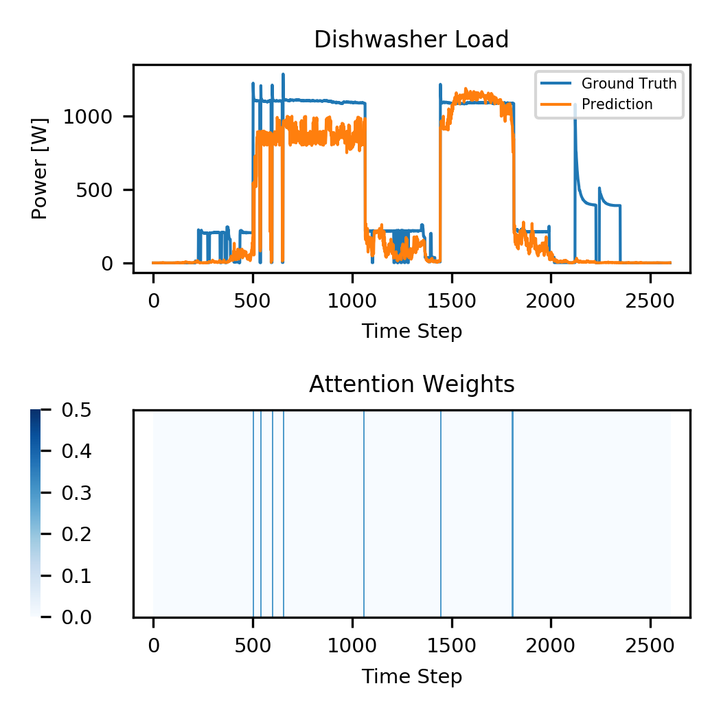
Figure 4: REDD dishwasher load and the heatmap of the attention weights at 3s resolution.

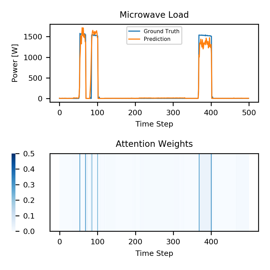
Figure 5: REDD microwave load and the heatmap of the attention weights at 3s resolution.

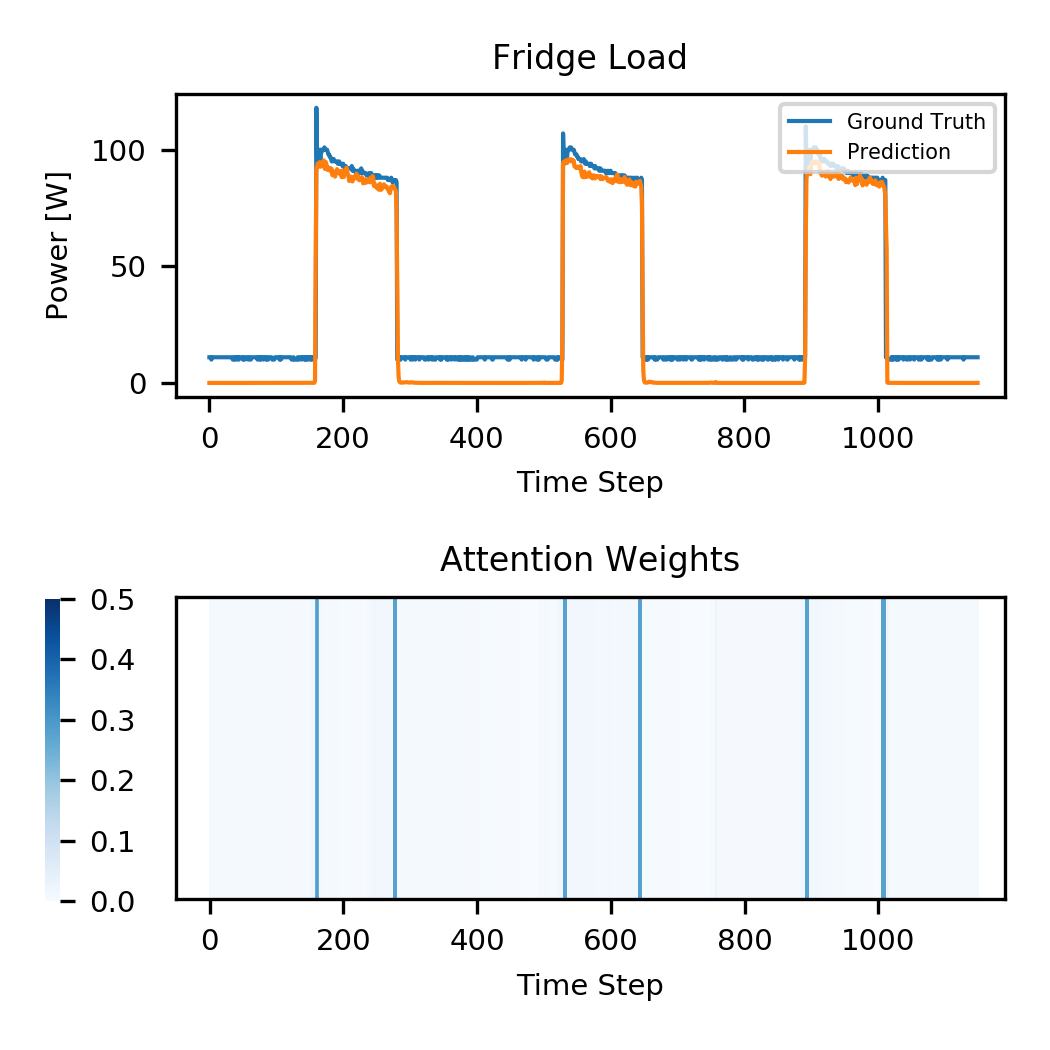
Figure 6: UK-DALE fridge load and the heatmap of the attention weights at 6s resolution.

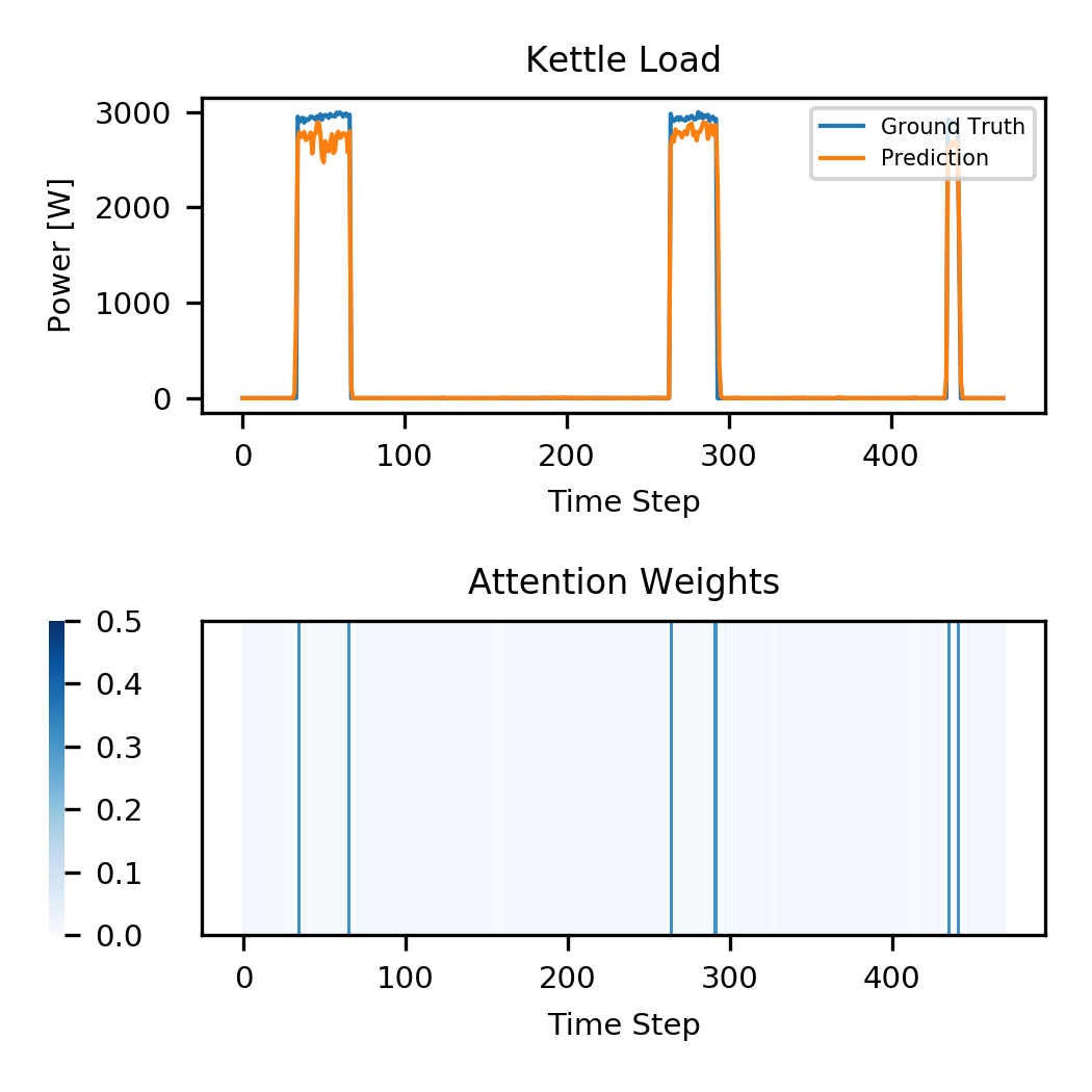
Figure 7: UK-DALE kettle load and the heatmap of the attention weights at 6s resolution.

References

- [1] G. W. Hart, “Nonintrusive appliance load monitoring,” Proceedings of the IEEE, vol. 80, no. 12, pp. 1870–1891, Dec 1992.
- [2] A. Ruano, A. Hernandez, J. Ureña, M. Ruano, and J. Garcia, “Nilm techniques for intelligent home energy management and ambient assisted living: A review,” Energies, vol. 12, no. 11, p. 2203, 2019.
- [3] W. A. de Souza, F. D. Garcia, F. P. Marafão, L. C. P. Da Silva, and M. G. Simões, “Load disaggregation using microscopic power features and pattern recognition,” Energies, vol. 12, no. 14, p. 2641, 2019.
- [4] A. Faustine, N. H. Mvungi, S. Kaijage, and K. Michael, “A survey on non-intrusive load monitoring methodies and techniques for energy disaggregation problem,” arXiv preprint arXiv:1703.00785, 2017.
- [5] A. Rahimpour, H. Qi, D. Fugate, and T. Kuruganti, “Non-intrusive energy disaggregation using non-negative matrix factorization with sum-to-k constraint,” IEEE Transactions on Power Systems, vol. 32, no. 6, pp. 4430–4441, 2017.
- [6] J. Z. Kolter and T. Jaakkola, “Approximate inference in additive factorial hmms with application to energy disaggregation,” in Artificial Intelligence and Statistics, 2012, pp. 1472–1482.
- [7] S. Makonin, F. Popowich, I. V. Bajić, B. Gill, and L. Bartram, “Exploiting HMM sparsity to perform online real-time nonintrusive load monitoring,” IEEE Transactions on smart grid, vol. 7, no. 6, pp. 2575–2585, 2015.
- [8] E. Nashrullah and A. Halim, “Performance Evaluation of Superstate HMM with Median Filter For Appliance Energy Disaggregation,” in 2019 6th International Conference on Electrical Engineering, Computer Science and Informatics (EECSI). IEEE, 2019, pp. 374–379.
- [9] K. Basu, V. Debusschere, S. Bacha, U. Maulik, and S. Bondyopadhyay, “Nonintrusive load monitoring: A temporal multilabel classification approach,” IEEE Transactions on industrial informatics, vol. 11, no. 1, pp. 262–270, 2014.
- [10] V. Singhal, J. Maggu, and A. Majumdar, “Simultaneous detection of multiple appliances from smart-meter measurements via multi-label consistent deep dictionary learning and deep transform learning,” IEEE Transactions on Smart Grid, vol. 10, no. 3, pp. 2969–2978, 2018.
- [11] S. Singh and A. Majumdar, “Non-Intrusive Load Monitoring via Multi-Label Sparse Representation-Based Classification,” IEEE Transactions on Smart Grid, vol. 11, no. 2, pp. 1799–1801, 2019.
- [12] A. Faustine and L. Pereira, “Multi-Label Learning for Appliance Recognition in NILM Using Fryze-Current Decomposition and Convolutional Neural Network,” Energies, vol. 13, no. 16, 2020. [Online]. Available: https://www.mdpi.com/1996-1073/13/16/4154
- [13] J. Kelly and W. Knottenbelt, “Neural nilm: Deep neural networks applied to energy disaggregation,” in Proceedings of the 2nd ACM International Conference on Embedded Systems for Energy-Efficient Built Environments, 2015, pp. 55–64.
- [14] W. He and Y. Chai, “An empirical study on energy disaggregation via deep learning,” in 2016 2nd International Conference on Artificial Intelligence and Industrial Engineering (AIIE 2016), 2016.
- [15] C. Zhang, M. Zhong, Z. Wang, N. Goddard, and C. Sutton, “Sequence-to-point learning with neural networks for non-intrusive load monitoring,” in Thirty-Second AAAI Conference on Artificial Intelligence, 2018.
- [16] R. Bonfigli, A. Felicetti, E. Principi, M. Fagiani, S. Squartini, and F. Piazza, “Denoising autoencoders for non-intrusive load monitoring: improvements and comparative evaluation,” Energy and Buildings, vol. 158, pp. 1461–1474, 2018.
- [17] C. Shin, S. Joo, J. Yim, H. Lee, T. Moon, and W. Rhee, “Subtask gated networks for non-intrusive load monitoring,” in Proceedings of the AAAI Conference on Artificial Intelligence, vol. 33, 2019, pp. 1150–1157.
- [18] K. Chen, Y. Zhang, Q. Wang, J. Hu, H. Fan, and J. He, “Scale-and context-aware convolutional non-intrusive load monitoring,” IEEE Transactions on Power Systems, 2019.
- [19] W. Kong, Z. Y. Dong, B. Wang, J. Zhao, and J. Huang, “A Practical Solution for Non-Intrusive Type II Load Monitoring Based on Deep Learning and Post-Processing,” IEEE Transactions on Smart Grid, vol. 11, no. 1, pp. 148–160, 2020.
- [20] K. Wang, H. Zhong, N. Yu, and Q. Xia, “Nonintrusive load monitoring based on sequence-to-sequence model with attention mechanism,” Zhongguo Dianji Gongcheng Xuebao/Proceedings of the Chinese Society of Electrical Engineering, vol. 39, pp. 75–83, 01 2019.
- [21] D. Bahdanau, K. Cho, and Y. Bengio, “Neural machine translation by jointly learning to align and translate,” arXiv preprint arXiv:1409.0473, 2014.
- [22] I. Sutskever, O. Vinyals, and Q. V. Le, “Sequence to sequence learning with neural networks,” in Advances in neural information processing systems, 2014, pp. 3104–3112.
- [23] K. Cho, B. Van Merriënboer, D. Bahdanau, and Y. Bengio, “On the properties of neural machine translation: Encoder-decoder approaches,” arXiv preprint arXiv:1409.1259, 2014.
- [24] T. Young, D. Hazarika, S. Poria, and E. Cambria, “Recent trends in deep learning based natural language processing,” ieee Computational intelligenCe magazine, vol. 13, no. 3, pp. 55–75, 2018.
- [25] C. Raffel and D. P. Ellis, “Feed-forward networks with attention can solve some long-term memory problems,” arXiv preprint arXiv:1512.08756, 2015.
- [26] J. Z. Kolter and M. J. Johnson, “Redd: A public data set for energy disaggregation research,” in Workshop on data mining applications in sustainability (SIGKDD), San Diego, CA, vol. 25, 2011, pp. 59–62.
- [27] J. Kelly and W. Knottenbelt, “The uk-dale dataset, domestic appliance-level electricity demand and whole-house demand from five uk homes,” Scientific data, vol. 2, p. 150007, 2015.
- [28] I. Sutskever, J. Martens, G. Dahl, and G. Hinton, “On the importance of initialization and momentum in deep learning,” in International conference on machine learning, 2013, pp. 1139–1147.
- [29] R. Caruana, S. Lawrence, and L. Giles, “Overfitting in neural nets: Backpropagation, conjugate gradient, and early stopping,” in Proceedings of the 13th International Conference on Neural Information Processing Systems, ser. NIPS’00. MIT Press, 2000, pp. 381–387.
- [30] A. Paszke, S. Gross, S. Chintala, G. Chanan, E. Yang, Z. DeVito, Z. Lin, A. Desmaison, L. Antiga, and A. Lerer, “Automatic differentiation in PyTorch,” in NIPS Autodiff Workshop, 2017.
- [31] N. Batra, J. Kelly, O. Parson, H. Dutta, W. Knottenbelt, A. Rogers, A. Singh, and M. Srivastava, “Nilmtk: an open source toolkit for non-intrusive load monitoring,” in Proceedings of the 5th international conference on Future energy systems, 2014, pp. 265–276.