Relating $\ell_{p}$ regularization and reweighted $\ell_{1}$ regularization

Abstract

We propose a general framework of iteratively reweighted $\ell_{1}$ methods for solving $\ell_{p}$ regularization problems. We prove that after some iteration $k$, the iterates generated by the proposed methods have the same support and sign as the limit points, and are bounded away from 0, so that the algorithm behaves like solving a smooth problem in the reduced space. As a result, the global convergence can be easily obtained and an update strategy for the smoothing parameter is proposed which can automatically terminate the updates for zero components. We show that $\ell_{p}$ regularization problems are locally equivalent to a weighted $\ell_{1}$ regularization problem and every optimal point corresponds to a Maximum A Posterior estimation for independently and non-identically distributed Laplace prior parameters. Numerical experiments exhibit the behaviors and the efficiency of our proposed methods.

90C06, 90C26, 90C30, 90C90, 49J52, 65K05, 49M37, 62J07

1 Introduction

In recent years, sparse regularization problems have attracted considerable attentions because of their wide applications, including machine learning [15, 18], statistics [12, 14] and compressed sensing [5, 23]. Sparse solutions generally lead to better generalization of the model performance from training data to future data. A common approach is the $\ell_{p}$ ($0\leq p\leq 1)$ regularization technique, which minimizes the loss function combined with a convex/nonconvex penalization term such as the $\ell_{p}$ norm of the model parameters. Nonconvex regularization technique with $0<p<1$ nowadays has become popular due to its power in promoting sparsity.

The primary focus of this paper is on analyzing the properties of nonconvex $\ell_{p}$ regularization, and designing efficient numerical algorithms for solving the $\ell_{p}$ regularized problem

(P) $$\underset{x\in\mathbb{R}^{n}}{\min} F(x):=f(x)+\lambda\psi(x)\quad\text{with }\psi(x)=\|x\|_{p}:=\left(\sum_{i=1}^{n}|x_{i}|_{p}\right)^{1/p}$$

where $f:\mathbb{R}^{n}\to\mathbb{R}$ is a continuously differentiable function, $p\in(0,1)$ and $\lambda>0$ is the regularization parameter. This technique is often regarded as a better approximation to the $\ell_{0}$ regularization than the $\ell_{1}$ regularization, and can often yield sparser solutions.

However, $\ell_{p}$ regularized problems are generally difficult to handle and analyze due to its nonconvex and non-Lipschitz continuous nature. In fact, Ge [11] proved that finding the global minimal value of the problem with $\ell_{p}$-norm $(0<p<1)$ regularization term is strongly NP-Hard. Therefore, many works focus on replacing the nonconvex and nonsmooth regularization term with trackable smooth approximation. For example, Chen et al. [7] approximate $|x_{i}|^{p}$ by a continuously differentiable function

$$\psi_{\mu}(x_{i})=\begin{cases}|x_{i}|,&|x_{i}|>\mu,\\ \dfrac{x_{i}^{2}}{2\mu}+\dfrac{\mu}{2},&|x_{i}|\leq\mu,\end{cases}$$

with $\mu\in\mathbb{R}_{+}$, which is solved by a hybrid orthogonal matching pursuit-smoothing gradient method. Lu [16] constructed another Lipschitz continuous approximation to $|x_{i}|^{p}$

(1) $$\psi_{\mu_{\epsilon}}(x_{i})=\begin{cases}|x_{i}|^{p},&|x_{i}|^{p}>\mu_{\epsilon};\vspace{0.1cm}\\ \mu_{\epsilon},&|x_{i}|^{p}\leq\mu_{\epsilon}.\end{cases}$$

with $\mu_{\epsilon}=\dfrac{\epsilon}{\lambda n}$ and then proposed an iteratively reweighed algorithm. Chen [6] proposed a smoothing trust region Newton algorithm for solving the approximated problem by replacing $|x_{i}|^{p}$ by

$$\psi_{\mu}(x_{i})=\left(x_{i}^{2}+4\mu^{2}\right)^{\frac{p}{2}}.$$

Another type of approximation technique is to add smoothing perturbation to each $|x_{i}|$, which mainly includes the $\epsilon$-approximation of (P)

(2) $$\psi_{\epsilon,1}(x_{i})=\left(|x_{i}|+\epsilon\right)^{p}\ \text{ and }\ \psi_{\epsilon,2}(x_{i})=\left(x_{i}^{2}+\epsilon\right)^{p/2}$$

by Chen and Zhou [8] and Lai and Wang [13] with prescribed small $\epsilon>0$.

Among these algorithms, iteratively reweighted methods [16, 20, 21] for solving approximation (2) are popular and proved to be efficient for many cases. At each iteration, it replaces (2) by

(3) $$p(|x_{i}^{k}|+\epsilon_{i})^{p-1}|x_{i}|\quad\text{or}\quad\tfrac{p}{2}((x^{k}_{i})^{2}+\epsilon_{i})^{\frac{p}{2}-1}x_{i}^{2},$$

respectively via linearizing $(\cdot)^{p}$ and $(\cdot)^{\frac{p}{2}}$ at $x^{k}$. In this problem, large $\epsilon$ will smooth out many local minimizers, while small values make the subproblems difficult to solve and easily trapped into bad local minimizers. In order to approximate Eq. P effectively, Lu [16] improved these weights by dynamically updating perturbation parameter $\epsilon_{i}$ at each iteration to better approximate original problem.

1.1 Key contributions

The contributions of this paper can be summarized below.

• We proposed a general framework of iteratively $\ell_{1}$ methods and studied the convergence, which can include different types of iteratively reweighted $\ell_{1}$ methods such as first-order and second-order methods.

• We showed that the proposed iteratively reweighed $\ell_{1}$ methods locally have the same support and sign of the iterates as the optimal solution when applied to non-Lipschitz regularization problems. Consequently, these methods locally behave like solving a smooth problem, which could potentially make the analysis for these algorithms easier and straightforward.

• We showed that the $\ell_{p}$ regularization problem is locally equivalent to a weighted $\ell_{1}$ regularization problem. That being said, any first-order optimal solution of $\ell_{p}$ regularization problem can be identified with the optimal solution of a weighted $\ell_{1}$ regularization problem which is equivalent to finding a mode of Maximum A Posterior (MAP) for independently and non-identically distributed Laplace prior on the parameters.

1.2 Notation

For $x\in\mathbb{R}^{n}$, let $x_{i}$ be the $i$th element of $x$, and define the support of $x$ as ${\cal I}(x)=\{i\mid x_{i}\neq 0\}$ and its complement as ${\cal A}(x)=\{i\mid x_{i}=0\}$. Denote $e$ as the vector of all 1s of appropriate dimension. The sign of $x\in\mathbb{R}^{n}$ is defined as $(\text{sign}(x))_{i}=\text{sign}(x_{i})$. For $H\in\mathbb{R}^{n\times n}$ and index sets ${\cal A},{\cal I}\subset\{1,\ldots,n\}$, let $H_{{\cal A},{\cal I}}$ be the matrix consisting of $h_{i,j},i\in{\cal A},j\in{\cal I}$, and $\text{diag}(a_{i},i\in{\cal A})$ be the diagonal matrix with the elements of vector $a_{i},i\in{\cal A}$ on the main diagonal. The componentwise product of two vectors $a\in\mathbb{R}^{n}$ and $b\in\mathbb{R}^{n}$ is defined as $(a\circ b)_{i}=a_{i}b_{i}$. Let $\{-1,0,+1\}^{n}$ be the set of $n$-dimensional vectors with components chosen from $\{-1,0,+1\}$.

In $\mathbb{R}^{n}$, denote $\|\cdot\|_{p}$ as the $\ell_{p}$ norm with $p\in(0,+\infty)$, i.e., $\|x\|_{p}=\left(\sum_{i=1}^{n}|x_{i}|^{p}\right)^{1/p}$. Note that for $p\in(0,1)$, this does not define a proper norm due to its lack of subadditivity. If function $f:\mathbb{R}^{n}\to\bar{\mathbb{R}}:=\mathbb{R}\cup\{+\infty\}$ is convex, then the subdiferential of $f$ at $\bar{x}$ is given by

$$\partial f(\bar{x}):=\{z\mid f(\bar{x})+\langle z,x-\bar{x}\rangle\leq f(x),\ \forall x\in\mathbb{R}^{n}\}.$$

In particular, for $x\in\mathbb{R}^{n}$, we use $\partial\|x\|_{1}$ to denote the set $\{\xi\in\mathbb{R}^{n}\mid\xi_{i}\in\partial|x_{i}|,i=1,\ldots,n\}.$ For closed convex set $\Omega\subset\mathbb{R}^{n}$, define the Euclidean distance of point $a\in\mathbb{R}^{n}$ to $\Omega$ as $\text{dist}(a,\Omega)=\min_{b\in\Omega}\|a-b\|_{2}$.

2 Iteratively reweighted $\ell_{1}$ methods

In this section, we introduce the framework of iteratively reweighted $\ell_{1}$ methods for solving (P). Given $\epsilon\in\mathbb{R}^{n}_{++}$, the iteratively reweighted $\ell_{1}$ method is based on smooth approximation $F(x,\epsilon)$ of $F(x)$

$$F(x,\epsilon):=f(x)+\lambda\sum_{i=1}^{n}(|x_{i}|+\epsilon_{i})^{p}.$$

We make the following assumption about $f$.

Assumption .

$f$ is Lipschitz differentiable with constant $L_{f}\geq 0$.

At $k$-th iteration, the algorithm formulates a convex local model to approximate $F(x)$

$$G(x;x^{k},\epsilon^{k}):=Q_{k}(x)+\lambda\sum_{i=1}^{n}w(x_{i}^{k},\epsilon_{i}^{k})|x_{i}|$$

where the weights are given by $w(x_{i}^{k},\epsilon_{i}^{k})=p(|x_{i}^{k}|+\epsilon_{i}^{k})^{p-1}.$ $Q_{k}(x)$ represents a local approximation model to $f$ at $x^{k}$, and is generally assumed to be smooth and convex. Common approaches include the following.

• Proximal first-order approximation: $Q_{k}(x)=\nabla f(x^{k})^{T}(x-x^{k})+\frac{\beta}{2}\|x-x^{k}\|_{2}^{2}$ with $\beta>0$.

• Quasi-Newton approximation: $Q_{k}(x)=\nabla f(x^{k})^{T}(x-x^{k})+\tfrac{1}{2}(x-x^{k})^{T}B^{k}(x-x^{k})$ with $B^{k}\in\mathbb{R}^{n\times n}$.

• Newton approximation: $Q_{k}(x)=\nabla f(x^{k})^{T}(x-x^{k})+\tfrac{1}{2}(x-x^{k})^{T}\nabla^{2}f(x^{k})(x-x^{k})$.

The next iterate $x^{k+1}$ is then computed as the solution of $\min_{x\in\mathbb{R}^{n}}G(x;x^{k},\epsilon^{k})$:

$$x^{k+1}\leftarrow\arg\min_{x\in\mathbb{R}^{n}}G(x;x^{k},\epsilon^{k})$$

with $\epsilon$ driven towards to 0: $\epsilon^{k+1}\leq\mu\epsilon^{k}$ and $\mu\in(0,1)$.

We state the framework of this iteratively reweighted $\ell_{1}$ method in Algorithm 1.

Algorithm 1 General framework of iteratively reweighted $\ell_{1}$ (IRL1) methods

1:  Input: $\mu\in(0,1),\epsilon^{0}\in\mathbb{R}^{n}_{++}$ and $x^{0}$.

2:  Initialize: set $k=0$.

3:  repeat

4:     Reweighing: $w(x_{i}^{k},\epsilon_{i}^{k})=p(|x^{k}_{i}|+\epsilon^{k}_{i})^{p-1}.$

5:     Compute new iterate: $x^{k+1}\leftarrow\underset{x\in\mathbb{R}^{n}}{\text{argmin}}\quad\bigg{\{}Q_{k}(x)+\lambda\sum\limits_{i=1}^{n}w(x_{i}^{k},\epsilon_{i}^{k})|x_{i}|\bigg{\}}.$

6:     Set $\epsilon^{k}\leq\mu\epsilon^{k-1}$, $k\leftarrow k+1$.

7:  until convergence

We make the following assumptions about the choice of $Q_{k}(\cdot)$.

Assumption .

The initial point $(x^{0},\epsilon^{0})$ and local convex model $Q_{k}(\cdot)$ are such that

1. The level set ${\cal L}(F^{0}):=\{x\mid F(x)\leq F^{0}\}$ is bounded where $F^{0}:=F(x^{0},\epsilon^{0})$.

2. For all $k\in\mathbb{N}$, $\nabla Q_{k}(x^{k})=\nabla f(x^{k})$, $Q_{k}(\cdot)$ is strongly convex with constant $M>L_{f}/2>0$, and Lipschitz differentiable with constant $L>0$.

This assumption is relatively loose on the local model $Q_{k}(\cdot)$. In particular, in the proximal method, this condition trivially holds. In the (quasi-)Newton approximation, it suffices to require $MI\preceq\nabla^{2}f(x^{k})\preceq LI$ ($MI\preceq B^{k}\preceq LI$). It should be noticed that in fact our analysis only relies on these conditions to hold on ${\cal L}(F^{0})$.

2.1 Monotonicity of $F(x,\epsilon)$

In this section, we show that $F(x,\epsilon)$ is monotonically decreasing over our iterates $(x^{k},\epsilon^{k})$. For the ease of presentation, we define the following two terms

$$\Delta F(x^{k+1},\epsilon^{k+1}):= F(x^{k},\epsilon^{k})-F(x^{k+1},\epsilon^{k+1})$$

$$\Delta G(x^{k+1};x^{k},\epsilon^{k}):= G(x^{k};x^{k},\epsilon^{k})-G(x^{k+1};x^{k},\epsilon^{k}),$$

and use the following shorthands $w_{i}^{k}:=w(x_{i}^{k},\epsilon_{i}^{k})\text{ and }W^{k}:=\text{diag}(w_{1}^{k},\ldots,w_{n}^{k}).$

Proposition 2.1.

Suppose Section 2 and 2 hold. Let $\{(x^{k},\epsilon^{k})\}$ be the sequence generated by Algorithm 1. It follows that $F(x,\epsilon)$ is monotonically decreasing over $\{(x^{k},\epsilon^{k})\}$ and the reduction satisfies

(4) $$F(x^{0},\epsilon^{0})-F(x^{k};\epsilon^{k}) \geq(M-\tfrac{L_{f}}{2})\sum_{t=0}^{k-1}\|x^{t+1}-x^{t}\|^{2}_{2}.$$

Moreover, $\lim\limits_{k\to\infty}\|x^{k+1}-x^{k}\|_{2}=0$, and there exists $C>0$ such that $\|\nabla Q_{k}(x^{k+1})\|_{\infty}\leq C$ for any $k\in\mathbb{N}$.

Proof 2.2.

From Section 2 and 2, we have

$$f(x^{k})-f(x^{k+1})\geq \ \nabla f(x^{k})^{T}(x^{k}-x^{k+1})-\frac{L_{f}}{2}\|x^{k}-x^{k+1}\|_{2}^{2}$$

$$Q_{k}(x^{k})-Q_{k}(x^{k+1})\leq \ \nabla f(x^{k})^{T}(x^{k}-x^{k+1})-\frac{M}{2}\|x^{k+1}-x^{k}\|_{2}^{2}.$$

It follows that

(5) $$f(x^{k})-f(x^{k+1})\geq Q_{k}(x^{k})-Q_{k}(x^{k+1})+\frac{M-L_{f}}{2}\|x^{k}-x^{k+1}\|_{2}^{2}.$$

On the other hand, the concavity of $a^{p}$ on $\mathbb{R}_{++}$ gives $a_{1}^{p}\leq a_{2}^{p}+pa_{2}^{p-1}(a_{1}-a_{2})$ for any $a_{1},a_{2}\in\mathbb{R}_{++}$, implying for $i=1,\ldots,n$

$$(|x_{i}^{k+1}|+\epsilon_{i}^{k})^{p}\leq \ (|x_{i}^{k}|+\epsilon_{i}^{k})^{p}+p(|x_{i}^{k}|+\epsilon_{i}^{k})^{p-1}(|x_{i}^{k+1}|-|x_{i}^{k}|)$$

$$= \ (|x_{i}^{k}|+\epsilon_{i}^{k})^{p}+w_{i}^{k}(|x_{i}^{k+1}|-|x_{i}^{k}|).$$

Summing the above inequality over $i$ yields

(6) $$\sum_{i=1}^{n}(|x_{i}^{k+1}|+\epsilon_{i}^{k})^{p}\leq\sum_{i=1}^{n}(|x_{i}^{k}|+\epsilon_{i}^{k})^{p}+\sum_{i=1}^{n}w_{i}^{k}(|x_{i}^{k+1}|-|x_{i}^{k}|).$$

Combining (5) and (6) gives

(7) $$\Delta F(x^{k+1},\epsilon^{k+1})\geq\Delta G(x^{k+1};x^{k},\epsilon^{k})+\frac{M-L_{f}}{2}\|x^{k}-x^{k+1}\|_{2}^{2}.$$

Section 2 implies the subproblem solution $x^{k+1}$ satisfies the optimality condition

(8) $$\nabla Q_{k}(x^{k+1})+\lambda W^{k}\xi^{k+1}=0$$

with $\xi^{k+1}\in\partial\|x^{k+1}\|_{1}$. Hence

(9) $$\ G(x^{k};x^{k},\epsilon^{k})-G(x^{k+1};x^{k},\epsilon^{k})$$

$$= \ Q_{k}(x^{k})-Q_{k}(x^{k+1})+\lambda\sum_{i=1}^{n}w_{i}^{k}(|x^{k}_{i}|-|x_{i}^{k+1}|)$$

$$\geq \ \nabla Q_{k}(x^{k+1})^{T}(x^{k}-x^{k+1})+\tfrac{M}{2}\|x^{k+1}-x^{k}\|_{2}^{2}+\lambda\sum_{i=1}^{n}w_{i}^{k}\xi_{i}^{k+1}(x^{k}_{i}-x_{i}^{k+1})$$

$$= \ [\nabla Q_{k}(x^{k+1})+\lambda W^{k}\xi^{k+1}]^{T}(x^{k}-x^{k+1})+\tfrac{M}{2}\|x^{k+1}-x^{k}\|_{2}^{2}$$

$$= \ \tfrac{M}{2}\|x^{k+1}-x^{k}\|_{2}^{2},$$

where the inequality is by Section 2 and the convexity of $|\cdot|$, and the last equality is by (8).

We then combine (7) and (9) to get

(10) $$\Delta F(x^{k+1},\epsilon^{k+1})\geq F(x^{k},\epsilon^{k})-F(x^{k+1},\epsilon^{k})\geq(M-\tfrac{L_{f}}{2})\|x^{k}-x^{k+1}\|_{2}^{2}.$$

Replacing $k$ with $t$ and summing up from $t=0$ to $k-1$, we have

$$\sum_{t=0}^{k-1}(F(x^{t},\epsilon^{t})-F(x^{t+1},\epsilon^{t+1}))\geq(M-\tfrac{L_{f}}{2})\sum_{k=0}^{k-1}\|x^{t}-x^{t+1}\|_{2}^{2},$$

completing the proof of (4).

It follows that $\{x^{k}\}\subset{\cal L}(F^{0})$ by $F(x^{k})\leq F(x^{k},\epsilon^{k})\leq F(x^{0},\epsilon^{0})$ by (4). By Section 2(i), it is bounded and $\liminf\limits_{k\to\infty}F(x^{k},\epsilon^{k})>-\infty$. Taking $k\to\infty$ in Eq. 7, we know

$$(M-\tfrac{L_{f}}{2})\sum_{i=0}^{\infty}\|x^{k+1}-x^{k}\|^{2}\leq F(x^{0},\epsilon^{0})-\liminf\limits_{k\to\infty}F(x^{k},\epsilon^{k})<\infty,$$

implying $\lim_{k\to\infty}\|x^{k+1}-x^{k}\|=0$. Moreover, it follows from the boundedness of $\{x^{k}\}$ that there must exist $C>0$ such that $\|Q_{k}(x^{k+1})\|_{\infty}\leq C$ for any $k\in\mathbb{N}$.

2.2 Locally stable sign

We now show that under Assumption 2, after some iteration, the support of the iterates remains unchanged. The result is summarized in the following theorem.

Theorem 2.3 (Locally stable support).

Assume Assumption 2 and 2 hold and let $\{(x^{k},\epsilon^{k})\}$ be a sequence generated by Algorithm 1. $C$ is the constant as defined in Proposition 2.1. Then we have the following

1. If $w(x_{i}^{\tilde{k}},\epsilon_{i}^{\tilde{k}})>C/\lambda$ for some ${\tilde{k}}\in\mathbb{N}$, then $x_{i}^{k}\equiv 0$ for all $k>\tilde{k}$. Conversely, if there exists $\hat{k}>\tilde{k}$ for any $\tilde{k}\in\mathbb{N}$ such that $x_{i}^{\hat{k}}\neq 0$, then $w(x_{i}^{k},\epsilon_{i}^{k})\leq C/\lambda$ for all $k\in\mathbb{N}$.

2. There exist index sets ${\cal I}^{*}\cup{\cal A}^{*}=\{1,\ldots,n\}$ and $\bar{k}>0$, such that $\forall\ k>\bar{k}$, ${\cal I}(x^{k})\equiv{\cal I}^{*}$ and ${\cal A}(x^{k})\equiv{\cal A}^{*}$.

3. For any $i\in{\cal I}^{*}$, it holds that

   (11) $$|x_{i}^{k}|>\left(\frac{C}{p\lambda}\right)^{\frac{1}{p-1}}-\epsilon_{i}^{k}>0,\quad i\in{\cal I}^{*}.$$

   Therefore, $\{|x_{i}^{k}|,i\in{\cal I}^{*},k\in\mathbb{N}\}$ are bounded away from 0 after some $\hat{k}\in\mathbb{N}$.

4. For any cluster point $x^{*}$ of $\{x^{k}\}$, it holds that ${\cal I}(x^{*})={\cal I}^{*}$, ${\cal A}(x^{*})={\cal A}^{*}$ and

   (12) $$|x^{*}_{i}|\geq\left(\frac{C}{p\lambda}\right)^{\frac{1}{p-1}},\quad i\in{\cal I}^{*}.$$

Proof 2.4.

(i) If $w(x_{i}^{\tilde{k}},\epsilon_{i}^{\tilde{k}})>C/\lambda$ for some ${\tilde{k}}\in\mathbb{N}$, then the optimality condition (8) implies $x_{i}^{{\tilde{k}}+1}=0$. Otherwise we have $|\nabla_{i}Q_{\tilde{k}}(x^{\tilde{k}+1})|=\lambda w(x_{i}^{\tilde{k}},\epsilon_{i}^{\tilde{k}})>C$, contradicting Proposition 2.1. Monotonicity of $(\cdot)^{p-1}$ and $0+\epsilon_{i}^{\tilde{k}+1}\leq|x_{i}^{\tilde{k}}|+\epsilon_{i}^{\tilde{k}}$ yield

$$w(x_{i}^{{\tilde{k}}+1},\epsilon_{i}^{{\tilde{k}}+1})=p(0+\epsilon_{i}^{{\tilde{k}}+1})^{p-1}\geq p(|x_{i}^{\tilde{k}}|+\epsilon_{i}^{\tilde{k}})^{p-1}=w(x_{i}^{\tilde{k}},\epsilon_{i}^{\tilde{k}})>C.$$

By induction we know that $x_{i}^{k}\equiv 0$ for any $k>\tilde{k}$. This completes the proof of (i).

(ii) Suppose by contradiction this statement is not true. There exists $j\in\{1,\ldots,n\}$ such that $\{x_{j}^{k}\}$ takes zero and nonzero values both for infinite times. Hence, there exists a subsequence ${\cal S}_{1}\cup{\cal S}_{2}=\mathbb{N}$ such that $|{\cal S}_{1}|=\infty$, $|{\cal S}_{2}|=\infty$ and that

$$x_{j}^{k}=0,\forall k\in{\cal S}_{1}\ \text{ and }\ x_{j}^{k}\neq 0,\forall k\in{\cal S}_{2}.$$

Since $\{\epsilon_{j}^{k}\}_{{\cal S}_{1}}$ is monotonically decreasing to 0, there exists $\tilde{k}\in{\cal S}_{1}$ such that

$$w(x_{j}^{\tilde{k}},\epsilon_{j}^{\tilde{k}})=p(|x_{i}^{\tilde{k}}|+\epsilon_{j}^{\tilde{k}})^{p-1}=p(\epsilon_{j}^{\tilde{k}})^{p-1}>C/\lambda.$$

It follows that $x_{j}^{k}\equiv 0$ for any $k>\tilde{k}$ by (i) which implies $\{\tilde{k}+1,\tilde{k}+2,\ldots\}\subset{\cal S}_{1}$ and $|{\cal S}_{2}|<\infty$. This violates the assumption $|{\cal S}_{2}|=\infty.$ Hence, (ii) is true.

(iii) Combining (i) and (ii), we know for any $i\in{\cal I}^{*}$, $w_{i}^{k}\leq C/\lambda$, which is equivalent to (11). This proves (iii).

(iv) For $i\in{\cal A}^{*}$, (ii) implies that $i\in{\cal A}(x^{*})$. For $i\in{\cal I}^{*}$, (ii) and (iii) imply that (12) is true, meaning $i\in{\cal I}(x^{*})$.

The above theorem indicates an interesting property of the iterates generated by Algorithm 1. All the cluster points of the iterates have the same support, so that we can use ${\cal I}^{*}={\cal I}(x^{*}),{\cal A}^{*}={\cal A}(x^{*})$. We continue to show the signs of $\{x^{k}\}$ also remain unchanged for sufficiently large $k$. Combined with Theorem 2.3, this means the iterates $\{x^{k}_{{\cal I}^{*}}\}$ will eventually stay in the interior of the same orthant. This result is shown in the following theorem.

Theorem 2.5 (Locally stable sign).

Suppose $\{x^{k}\}$ be a sequence generated by Algorithm 1 and Assumptions 2 and 2 are satisfied. There exists $\bar{k}\in\mathbb{N}$, such that the sign of $\{x^{k}\}$ are fixed for any $k>\bar{k}$, i.e., $\text{sign}(x^{k})\equiv s$ for some $s\in\{-1,0,+1\}^{n}$.

Proof 2.6.

From Theorem 2.3, we only have to show that the sign of $x_{i}^{k},i\in{\cal I}^{*}$ is fixed for sufficiently large $k$. By Proposition 2.1 and Theorem 2.3(iii), there exists $\bar{k}\in\mathbb{N}$, such that for any $k>\bar{k}$

(13) $$\ \|x^{k+1}-x^{k}\|_{2}<\ \bar{\epsilon}:=\frac{1}{2}\left(\frac{C}{p\lambda}\right)^{\frac{1}{p-1}}$$

(14) and $$\ |x_{i}^{k}|>\ \bar{\epsilon},\quad\forall i\in{\cal I}^{*}.$$

We prove this by contradiction. Assume there exists $j\in{\cal I}^{*}$ such that the sign of $x_{j}$ changes after $\bar{k}$. Hence there must be $\hat{k}\geq\bar{k}$ such that $x_{j}^{\hat{k}}x_{j}^{\hat{k}+1}<0$. It follows that

$$\|x^{\hat{k}+1}-x^{\hat{k}}\|_{2}\geq|x_{j}^{\hat{k}+1}-x_{j}^{\hat{k}}|=\sqrt{(x_{j}^{\hat{k}+1})^{2}+(x_{j}^{\hat{k}})^{2}-2x_{j}^{\hat{k}}x_{j}^{\hat{k}+1}}>\sqrt{\bar{\epsilon}^{2}+\bar{\epsilon}^{2}}=\sqrt{2}\bar{\epsilon},$$

where the last inequality is by Eq. 14. This contradicts with (13), completing the proof.

The locally stable support and sign of the iterates imply that for sufficiently large $k$, the algorithm is equivalent to solving a smooth problem in the reduced space $\mathbb{R}^{{\cal I}^{*}}$. Our analysis in the remainder of this paper is based on this observation.

2.3 Global convergence

We now provide the convergence of the framework of iteratively weighted $\ell_{1}$ method.

The first-order necessary condition [16] of (P) is

(15) $$\nabla_{i}f(x^{*})+\lambda p|x_{i}^{*}|^{p-1}\text{sign}(x_{i}^{*})=0\quad\text{for}\quad i\in{\cal I}(x^{*}).$$

The following theorem shows that every limit point of the iterates is a first-order stationary solution.

Theorem 2.7.

Suppose Section 2 and 2 hold. Let $\{x^{k}\}$ be a sequence generated by Algorithm 1 and $\Omega$ be the set of limit points of $\{x^{k}\}$. Then $\Omega\neq\emptyset$ and any $x^{*}\in\Omega$ is first-order optimal for Eq. P. Moreover, any $x^{*}\in\Omega$ with ${\cal A}(x^{*})\neq\emptyset$ is not a maximizer of Eq. P.

Proof 2.8.

Boundedness of ${\cal L}(F^{0})$ from Section 2 implies $\Omega\neq\emptyset$. Let $x^{*}$ be a limit point of $\{x^{k}\}$ with subsequence $\{x^{k}\}_{{\cal S}}\to x^{*}$. From Theorem 2.3 and 2.5, there exists $\bar{k}\in\mathbb{N}$ such that for any $k>\bar{k}$, the sign of $x^{k}$ stays the same.

Optimality condition of subproblem yields

$$\nabla_{i}Q_{k}(x^{k+1})+\lambda p(|x_{i}^{k}|+\epsilon_{i}^{k})^{p-1}\text{sign}(x_{i}^{k+1})=0,\quad i\in{\cal I}(x^{*}).$$

Taking the limit on ${\cal S}$, we have for each $i\in{\cal I}(x^{*})$,

$$0= \lim_{k\to\infty\atop k\in{\cal S}}|\nabla_{i}Q_{k}(x^{k+1})+\lambda p(|x_{i}^{k}|+\epsilon_{i}^{k})^{p-1}\text{sign}(x_{i}^{k+1})|$$

$$\geq \lim_{k\to\infty\atop k\in{\cal S}}|\nabla_{i}Q_{k}(x^{k})+\lambda p(|x_{i}^{k}|+\epsilon_{i}^{k})^{p-1}\text{sign}(x_{i}^{k})|-|\nabla_{i}Q_{k}(x^{k+1})-\nabla_{i}Q_{k}(x^{k})|$$

$$\geq \lim_{k\to\infty\atop k\in{\cal S}}|\nabla_{i}Q_{k}(x^{k})+\lambda p(|x_{i}^{k}|+\epsilon_{i}^{k})^{p-1}\text{sign}(x_{i}^{k})|-\|\nabla Q_{k}(x^{k+1})-\nabla Q_{k}(x^{k})\|_{1}$$

$$\geq \lim_{k\to\infty\atop k\in{\cal S}}|\nabla_{i}Q_{k}(x^{k})+\lambda p(|x_{i}^{k}|+\epsilon_{i}^{k})^{p-1}\text{sign}(x_{i}^{k})|-\sqrt{n}\|\nabla Q_{k}(x^{k+1})-\nabla Q_{k}(x^{k})\|_{2}$$

$$\geq \lim_{k\to\infty\atop k\in{\cal S}}|\nabla_{i}f(x^{k})+\lambda p(|x_{i}^{k}|+\epsilon_{i}^{k})^{p-1}\text{sign}(x_{i}^{k})|-\sqrt{n}L\|x^{k+1}-x^{k}\|_{2}$$

$$= \ \nabla_{i}f(x^{*})+\lambda p|x_{i}^{*}|^{p-1}\text{sign}(x_{i}^{*}),$$

where the second inequality is due to

$$\|\nabla Q_{k}(x^{k+1})-\nabla Q_{k}(x^{k})\|_{2}\leq L\|x^{k+1}-x^{k}\|_{2},$$

by Proposition 2.1 and Assumption 2. Therefore, $x^{*}$ is first-order optimal.

2.4 Uniqueness of limit points

By Theorem 2.3 and 2.5, $x^{k}_{{\cal I}^{*}}\equiv 0$ for sufficiently, meaning the IRL1 algorithm behaves like solving a smooth problem on the reduced space $\mathbb{R}^{{\cal I}^{*}}$ . We can thus derive various conditions that guarantee the uniqueness of the limit points. For example, we can show the uniqueness of limit points under Kurdyka-Łojasiewicz (KL) property [1, 4] of $F$, which is generally believed to be a weak assumption needed in the analysis for many algorithms. However, due to limit of space, we only provide the following sufficient condition to guarantee the uniqueness of a limit point $x^{*}$ of $\{x^{k}\}$.

Theorem 2.9.

Suppose Section 2 and 2 are true. Then $\{x^{k}\}$ either has a unique limit point, or its limit points form a compact connected set contained in the same orthant on which the objective has the same value. In particular, at a limit point $x^{*}$, if $[\nabla^{2}f(x^{*})]_{{\cal I}^{*},{\cal I}^{*}}+\lambda diag(\text{sign}(x_{i}^{*})p(p-1)(x_{i}^{*})^{p-2},i\in{\cal I}^{*})$ is nonsingular, then $x^{*}$ is the unique limit point.

Proof 2.10.

If there exist multiple cluster points for $F([x_{{\cal I}^{*}};0_{{\cal A}^{*}}])$, we have from $\|x^{k+1}-x^{k}\|_{2}\to 0$ by Proposition 2.1 and [3, Lemma 2.6] that the set of cluster points of $\{x^{k}\}$ is a compact connected set.

On the other hand, it is obvious that for any $x^{*}\in\Omega$ satisfying (15), $x^{*}_{{\cal I}^{*}}$ is the optimal solution of the reduced problem of $\ell_{p}$ regularization

$$\min_{x_{{\cal I}^{*}}\in\mathbb{R}^{{\cal I}^{*}}}\ F([x_{{\cal I}^{*}};0_{{\cal A}^{*}}]):=f([x_{{\cal I}^{*}};0_{{\cal A}^{*}}])+\lambda\sum_{i\in{\cal I}^{*}}|x_{i}|^{p}.$$

By [17, Theorem 7.3.5], if

$$[\nabla^{2}F([x_{{\cal I}^{*}};0_{{\cal A}^{*}}])]_{{\cal I}^{*},{\cal I}^{*}}=[\nabla^{2}f(x^{*})]_{{\cal I}^{*},{\cal I}^{*}}+\lambda diag(\text{sign}(x_{i}^{*})p(p-1)(x_{i}^{*})^{p-2},i\in{\cal I}^{*})$$

is nonsingular at $x_{{\cal I}^{*}}^{*}$, then $x^{*}$ is an isolated critical point. However, we have shown that $\Omega^{*}$ is a compact connected set and each element is a critical point—a contradiction. Therefore, $x^{*}$ must be the unique limit point.

2.5 Smart $\epsilon$ updating strategies

For iteratively reweighted methods, it is helpful to start with a relatively large $\epsilon$ and gradually reduce it to 0, since this may prevent the algorithm from quickly getting trapped into a local minimum. However, as the iteration proceeds, we need to let $\epsilon_{i}\to 0,i\in{\cal I}(x^{*})$ to obtain convergence, and keep $\epsilon_{i}\to 0,i\in{\cal A}(x^{*})$ updated slowly or even fixed after some iterations to prevent potential numerical issues or from becoming stuck at a local minimum. Such a strategy may need the estimate of ${\cal I}(x^{*})$ and ${\cal A}(x^{*})$, which are generally unknown at the beginning.

The updating strategy, named as “smart reweighting”, is as follows.

(SR) $$\boxed{\begin{cases}\epsilon_{i}^{k+1}=\ \ \epsilon_{i}^{k}&\quad\text{ if }\ x_{i}^{k+1}=0,\\ \epsilon_{i}^{k+1}\leq\mu\epsilon_{i}^{k}&\quad\text{ if }\ x_{i}^{k+1}\neq 0.\end{cases}}$$

If we update $\epsilon$ in Algorithm 1 according to (SR), one can easily see that Proposition 2.1 still holds true. Furthermore, we have the following results.

Theorem 2.11.

Suppose Section 2 and 2 are true, and $\{x^{k}\}$ are generated by Algorithm 1 with $\epsilon$ updated according to (SR). The following hold true

1. if $\lim\limits_{k\to\infty}\epsilon_{i}^{k}\to 0$, then $\liminf\limits_{k\to\infty}|x_{i}^{k}|>0$;

2. if $\lim\limits_{k\to\infty}\epsilon_{i}^{k}>0$ meaning $\epsilon_{i}$ is not updated after some iteration $\tilde{k}$, then $\lim\limits_{k\to\infty}x_{i}^{k}=0$.

3. if $\epsilon_{i}^{k}\equiv\epsilon_{i}^{\tilde{k}}$, then $w_{i}^{\tilde{k}}\geq\limsup\limits_{k\to\infty}\frac{|\nabla_{i}f(x^{k})|}{\lambda}$ and $\epsilon_{i}^{\tilde{k}}\leq\liminf\limits_{k\to\infty}\left(\frac{p\lambda}{|\nabla_{i}f(x^{k})|}\right)^{\frac{1}{1-p}}$.

Proof 2.12.

(i) If $\epsilon^{k}_{i}\to 0$, assume by contradiction there exists ${\cal S}\subset\mathbb{N}$ such that $\{|x_{i}^{k}|\}_{{\cal S}}\to 0$. It follows that $\{w_{i}^{k}\}_{{\cal S}}\to\infty$ since $\epsilon^{k}_{i}\to 0$. Therefore, there exists sufficiently large $\tilde{k}\in{\cal S}$, such that $w(x_{i}^{\tilde{k}},\epsilon_{i}^{\tilde{k}})>C/\lambda$ for some ${\tilde{k}}\in\mathbb{N}$; then the optimality condition (8) implies $x_{i}^{{\tilde{k}}+1}=0$. Otherwise we have $|\nabla_{i}Q_{\tilde{k}}(x^{\tilde{k}+1})|=\lambda w(x_{i}^{\tilde{k}},\epsilon_{i}^{\tilde{k}})>C$, contradicting Proposition 2.1. Monotonicity of $(\cdot)^{p-1}$ and $0+\epsilon_{i}^{\tilde{k}+1}\leq|x_{i}^{\tilde{k}}|+\epsilon_{i}^{\tilde{k}}$ yield

$$w(x_{i}^{{\tilde{k}}+1},\epsilon_{i}^{{\tilde{k}}+1})=p(0+\epsilon_{i}^{{\tilde{k}}+1})^{p-1}\geq p(|x_{i}^{\tilde{k}}|+\epsilon_{i}^{\tilde{k}})^{p-1}=w(x_{i}^{\tilde{k}},\epsilon_{i}^{\tilde{k}})>C.$$

By induction we know that $x_{i}^{k}\equiv 0$ for any $k>\tilde{k}$. Therefore, $\epsilon_{i}^{k}$ is not updated for all $k>\tilde{k}$ according to (SR)—a contradiction. Therefore, $\liminf_{k\to\infty}|x_{i}^{k}|>0$.

(ii) If $\epsilon^{k}_{i}$ is bounded away from 0, meaning it is never reduced after some iteration $\tilde{k}$, then we know $x_{i}^{k}\equiv 0$ for all $k>\tilde{k}$.

(iii) if $\epsilon_{i}^{k}$ is not updated after $\tilde{k}$, it means $x_{i}^{k}\equiv 0$ for any $k>\tilde{k}$. Therefore, by the optimality condition of the subproblem, we have $|\nabla_{i}Q_{k}(x^{k+1})|\leq w_{i}^{\tilde{k}}$ for all $k>\tilde{k}$, meaning (iii) is true.

It is easy to verify the analysis in §2 still holds true, and any limit point is still first-order optimal for (P).

2.6 Line search

The satisfaction of Section 2(ii) by Algorithm 1 could be impractical since it requires the prior knowledge of the Lipschitz constant $L_{f}$ of $f$. In this subsection, we propose a line search strategy that still guarantee the convergence of IRL1 without knowing the value of $L_{f}$. Notice that the purpose of requiring $M$ to satisfy Section 2(ii) is to guarantee (5) in the proof of Proposition 2.1. Alternatively, we can directly require the model $Q_{k}(\cdot)$ yields a new iterate $x^{k+1}$ satisfying a similar condition

(16) $$f(x^{k})-f(x^{k+1})\geq Q_{k}(x^{k})-Q_{k}(x^{k+1})+\gamma\|x^{k}-x^{k+1}\|_{2}^{2}$$

for prescribed $\gamma>0$. To achieve this, we can repeatedly solve the subproblem and convexify the subproblem $Q_{k}$ by adding a proximal term to $Q_{k}(\cdot)$ if (16) is not satisfied, i.e., setting

$$Q_{k}(x)\leftarrow\ Q_{k}(x)+\tfrac{\Gamma}{2}\|x-x^{k}\|^{2}_{2}.$$

Algorithm 2 General framework of IRL1 methods with line search (IRL1-LS)

1:  Input: $\mu\in(0,1),\gamma\in(0,+\infty),\epsilon^{0}\in\mathbb{R}^{n}_{++}$ and $x^{0}$.

2:  Initialize: set $k=0$.

3:  repeat

4:     Reweighing: $w(x_{i}^{k},\epsilon_{i}^{k})=p(|x^{k}_{i}|+\epsilon^{k}_{i})^{p-1}.$

5:     Line search: find the smallest $\Gamma\geq 0$ such that

$$Q_{k}(x)\leftarrow \ Q_{k}(x)+\tfrac{\Gamma}{2}\|x-x^{k}\|^{2}_{2}$$

$$x^{k+1}\leftarrow \ \underset{x\in\mathbb{R}^{n}}{\text{argmin}}\quad\bigg{\{}Q_{k}(x)+\lambda\sum\limits_{i=1}^{n}w(x_{i}^{k},\epsilon_{i}^{k})|x_{i}|\bigg{\}}$$

$$f(x^{k})-f(x^{k+1})\geq \ Q_{k}(x^{k})-Q_{k}(x^{k+1})+\gamma\|x^{k}-x^{k+1}\|_{2}^{2}.$$

6:     Set $\epsilon^{k}\leq\mu\epsilon^{k-1}$, $k\leftarrow k+1$.

7:  until convergence

We state the IRL1 method with line search (IRL1-LS) in Algorithm 2, where the appropriate value of $\Gamma$ could be selected as the smallest element in $\{0,\bar{\Gamma}^{0},\bar{\Gamma}^{1},\bar{\Gamma}^{2},\ldots\}$ with given $\bar{\Gamma}>1$ such that (5) is true. This needs the solution of several additional subproblems for each iteration. Obviously, this line search procedure will terminate in finite trials since (5) is always satisfied for any $M>L_{f}+2\gamma$. Replacing (5) by (16) in the proof of Proposition 2.1, we can obtain similar result to Proposition 2.1 as below.

Proposition 2.13.

Suppose Section 2 and 2(i) hold. Let $\{(x^{k},\epsilon^{k})\}$ be the sequence generated by Algorithm 2. It follows that $F(x,\epsilon)$ is monotonically decreasing over $\{(x^{k},\epsilon^{k})\}$ and the reduction satisfies

(17) $$F(x^{0},\epsilon^{0})-F(x^{k};\epsilon^{k}) \geq\gamma\sum_{i=0}^{k-1}\|x^{k+1}-x^{k}\|^{2}_{2}.$$

Moreover, $\lim\limits_{k\to\infty}\|x^{k+1}-x^{k}\|_{2}=0$, and there exists $C>0$ such that $\|\nabla Q_{k}(x^{k+1})\|_{\infty}\leq C$ for any $k\in\mathbb{N}$.

Using Proposition 2.13, all the results in subsections 2.2–2.5 still hold true, which can be verified trivially and are therefore skipped.

3 Connection with weighted $\ell_{1}$ regularization

From what we have obtained from previous sessions, we can claim that

$$\boxed{\ell_{p}\text{ regularization is locally equivalent to a weighted $\ell_{1}$ regularization}}$$

with $p\in(0,1]$. This result is summarized below.

Theorem 3.1.

Any point $x^{*}$ satisfying the first-order necessary condition (15) of (P) is also optimal for the weighted $\ell_{1}$ regularization problem

(18) $$\min_{x\in\mathbb{R}^{n}}f(x)+\lambda\sum_{i=1}^{n}w_{i}|x_{i}|,$$

with weights $w_{i}=p|x_{i}^{*}|^{p-1},i\in{\cal I}(x^{*})$ and $w_{i}>|\nabla_{i}f(x^{*})|/\lambda,i\in{\cal A}(x^{*})$.

This relationship between $\ell_{p}$ and weighted $\ell_{1}$ regularizations is demonstrated in Figure 1. The contour of the weighted $\ell_{1}$ regularization problem is very similar to that of the $\ell_{0.5}$ regularization problem around the optimal solution, and they both attain minimum at the same point. For $\ell_{1}$ regularization, the contour is different from $\ell_{0.5}$ and it does not attain minimum at the same point as $\ell_{0.5}$.

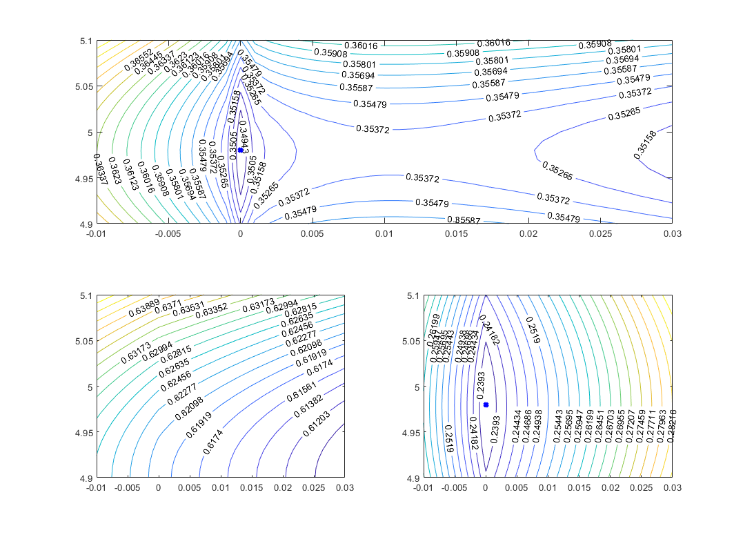
Figure 1: Upper: the contour of $\ell_{p}$ ($p=0.5$) regularization problem with $F(x)=(x_{1}-0.5)^{2}+(x_{2}-5)^{2}+0.1\|x\|_{p}^{p}$. Bottom left: contour of $F(x)=(x_{1}-0.5)^{2}+(x_{2}-5)^{2}+0.1\|x\|_{1}$. Bottom right: contour of $F(x)=(x_{1}-0.5)^{2}+(x_{2}-5)^{2}+0.1(20|x_{1}|+p(4.98)^{p-1}|x_{2}|)$. The $\ell_{p}$ and weighted $\ell_{1}$ problems attain optimality at the same sparse solution $(0,0.48)$. The $\ell_{1}$ problem does not have sparse optimal solution.

3.1 Maximum A Posterior (MAP)

It is well known [2, 19] that least squares with $\ell_{1}$ regularization is equivalent to finding a mode of posterior distribution for a linear Gaussian model with i.i.d. Laplace prior

$$y=Ax+\theta,\text{ where }A\in\mathbb{R}^{m\times n}\text{ and }\theta\sim N(0,\sigma^{2}I_{m}),$$

with $x_{i}\sim Laplace(0,b)$ for $i=1,\ldots,n$. The solution of MAP is as follows

$$\hat{x}=\arg\max_{x}\ \log p(x|A,y,b)=\arg\min_{x}\tfrac{1}{2}\|Ax-y\|_{2}^{2}+\frac{\sigma^{2}}{b}\|x\|_{1}.$$

In this case, it can be shown that the MAP estimator for the linear model with Laplace prior is the optimal solution of

$$\min_{x}\tfrac{1}{2}\|Ax-y\|_{2}^{2}+\frac{\sigma^{2}}{b}\|x\|_{1}.$$

Now suppose $x^{*}$ is a first-order optimal solution for the $\ell_{p}$ regularized least squares

(19) $$\underset{x\in\mathbb{R}^{n}}{\min} \tfrac{1}{2}\|Ax-y\|_{2}^{2}+\lambda\sum_{i=1}^{n}|x|_{p}^{p}.$$

Correspondingly, we consider a linear Gaussian model with $\sigma^{2}=\lambda$ and $x_{i}\sim Laplace(0,b_{i})$, $i=1,\ldots,n$ be independent Laplace distributions with

$$b_{i}=p|x_{i}^{*}|^{1-p},i\in{\cal I}(x^{*})\quad\text{and}\quad b_{i}\leq\lambda/|\nabla_{i}f(x^{*})|,i\in{\cal A}(x^{*}).$$

Then the solution of MAP is as follows

(20) $$\hat{x}=\arg\min_{x}\log p(x|A,y,b)=\arg\min_{x}\tfrac{1}{2}\|Ax-y\|_{2}^{2}+\sigma^{2}\sum_{i=1}^{n}\tfrac{1}{b_{i}}|x_{i}|.$$

It can be seen that the MAP estimator for the linear model with independent and non-identical Laplace prior is the optimal solution of

(21) $$\underset{x\in\mathbb{R}^{n}}{\min} \tfrac{1}{2}\|Ax-y\|_{2}^{2}+\sigma^{2}\sum_{i=1}^{n}\tfrac{1}{b_{i}}|x_{i}|.$$

Therefore, $x^{*}$ corresponds with a MAP estimator for the linear model with independent and non-identical Laplace prior defined above. If we apply an IRL1 to solve (19) with using the updating strategy (SR), then the limit point of the weights $w_{i}^{*}$ yields an estimate of the $b_{i}$ in such a MAP model, i.e., $\hat{b}_{i}=1/w_{i}^{*}$.

4 Numerical results

In this section, we perform sparse signal recovery experiments (similar to [24, 25, 10, 22]) to investigate the behavior of IRL1 for solving $\ell_{p}$ problem.

4.1 Experiment Setup

We generate an $m\times n$ matrix $A$ with i.i.d. $\mathcal{N}(0,1/m)$ entries. Then set $y=Ax_{true}+e$, where the origin signal $x_{true}$ contains $K$ randomly placed $\pm 1$ spikes and $e\in\mathbb{R}^{m}$ is i.i.d. $\mathcal{N}(0,10^{-4})$.

We test Algorithm 2 for small size problems with $(m,n,K)=(256,512,64)$ and large size problems $(m,n,K)=(1024,2048,256)$. All experiments start from origin and have the same termination criteria that

$$\max_{i\in\mathcal{I}(x)}|\nabla_{i}f(x)+\lambda p|x_{i}|^{p-1}\text{sign}(x_{i})|\leq\texttt{opttol},$$

where opttol$=10^{-6}$ is the prescribed tolerance. We also terminated if the maximum iteration number 500 is reached. Unless otherwise mentioned, we use the following parameters to run the experiments $\mu=0.9,\beta=0.1,\epsilon_{0}=1,\bar{\Gamma}=1.1,\gamma=0.0001,p=0.5\text{ and }\lambda=0.05$; $\epsilon$ is updated using the (SR) strategy.

4.2 Locally stable support

In this subsection, we run experiments to see the number of iterations the algorithm needs to find the stable support as shown in Theorem 2.3. Let $N_{S}$ be the iteration number for the support to be stabilized, $N$ be the final iteration number to reach the termination criteria. Then, the ratio $N_{S}/N$ shows at which stage the iterate starts to obtain the stable support.

The histogram of $N_{S}/N$ for 1000 problems of each size is shown in Fig. 2. The plot shows that the algorithm is able to reach the stable support stage in less than $50\%$ of final iterations for $98\%$ of problems. This means the stable support is identified at relatively early stage during the problem solving.

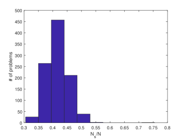
(a) The histogram about $N_{s}/N$ for small size problems.

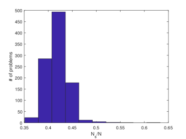
(b) The histogram about $N_{s}/N$ for large size problems.

Figure 2: The property of locally stable support for different size problems.

4.3 The impact of epsilon updating strategy

In this subsection, we test the benefits brought by our proposed $\epsilon$ updating strategy (SR). We compare updating strategy $\epsilon^{k+1}=\mu\epsilon^{k}$ against (SR) updating strategy on 1000 simulated problems of each size as mentioned in experiment setup section.

We plot the cumulative curve of the percentage of success cases over iteration number in Fig. 3. It clearly shows (SR) updating strategy outperforms $\epsilon^{k+1}=\mu\epsilon^{k}$ updating. Specifically, the (SR) updating strategy has $90\%$ problems solved within $260$ iterations compared with around $400$ for $\epsilon^{k+1}=\mu\epsilon^{k}$ updating. Besides, the (SR) updating strategy solve all 1000 problems, while around $6\%$ of the problems are still unsolved for $\epsilon^{k+1}=\mu\epsilon^{k}$ updating.

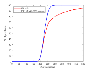
(a) The percentage of problems reaching termination criteria for small size problems

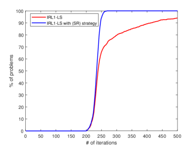
(b) The percentage of problems reaching termination criteria for large size problems

Figure 3: Comparison with different update strategies.

4.4 The impact of epsilon initialization

In this experiment, we set $\epsilon_{0}=$ 0.001, 0.005, 0.01 and 0.1 to see how the initialization of $\epsilon$ impact the convergence.

We plot the number of problems converging to a solution with the correct support (satisfy $\mathcal{I}(x_{true})=\mathcal{I}(x^{*})$) in Fig. 4. We make the following observation

• Larger $\epsilon_{0}$ has higher probability converge to the global optimal support.

• If $\epsilon_{0}$ is too small, the algorithm will get trapped to some bad local solution. In our experiment, when $\epsilon_{0}=0.001$, there is no problem finding the correct support.

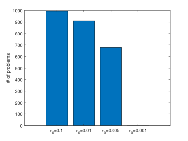
(a) The number of small size problems satisfying $\mathcal{I}(x_{true})=\mathcal{I}(x^{*})$.

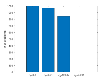
(b) The number of large size problems satisfying $\mathcal{I}(x_{true})=\mathcal{I}(x^{*})$.

Figure 4: The result of different epsilon initialization. It shows that the number of problems finding correct support over 1000 problems when $\epsilon_{0}=0.001,0.005,0.01,0.1$.

References

- [1] H. Attouch, J. Bolte, and B. F. Svaiter, Convergence of descent methods for semi-algebraic and tame problems: proximal algorithms, forward–backward splitting, and regularized gauss–seidel methods, Mathematical Programming, 137 (2013), pp. 91–129.
- [2] S. D. Babacan, R. Molina, and A. K. Katsaggelos, Bayesian compressive sensing using laplace priors, IEEE Transactions on Image Processing, 19 (2010), pp. 53–63, https://doi.org/10.1109/TIP.2009.2032894.
- [3] H. H. Bauschke, M. N. Dao, and W. M. Moursi, On fej’er monotone sequences and nonexpansive mappings, arXiv preprint arXiv:1507.05585, (2015).
- [4] J. Bolte, S. Sabach, and M. Teboulle, Proximal alternating linearized minimization for nonconvex and nonsmooth problems, Mathematical Programming, 146 (2014), pp. 459–494.
- [5] E. J. Candes, M. B. Wakin, and S. P. Boyd, Enhancing sparsity by reweighted minimization, Journal of Fourier analysis and applications, 14 (2008), pp. 877–905.
- [6] X. Chen, L. Niu, and Y.-X. Yuan, Optimality conditions and a smoothing trust region newton method for nonlipschitz optimization, SIAM Journal on Optimization, 23 (2013), pp. 1528–1552.
- [7] X. Chen, F. Xu, and Y. Ye, Lower bound theory of nonzero entries in solutions of minimization, SIAM Journal on Scientific Computing, 32 (2010), pp. 2832–2852.
- [8] X. Chen and W. Zhou, Convergence of reweighted minimization algorithms and unique solution of truncated lp minimization, Department of Applied Mathematics, The Hong Kong Polytechnic University, (2010).
- [9] I. Daubechies, M. Defrise, and C. De Mol, An iterative thresholding algorithm for linear inverse problems with a sparsity constraint, Communications on Pure and Applied Mathematics: A Journal Issued by the Courant Institute of Mathematical Sciences, 57 (2004), pp. 1413–1457.
- [10] M. A. Figueiredo, R. D. Nowak, and S. J. Wright, Gradient projection for sparse reconstruction: Application to compressed sensing and other inverse problems, IEEE Journal of selected topics in signal processing, 1 (2007), pp. 586–597.
- [11] D. Ge, X. Jiang, and Y. Ye, A note on the complexity of minimization, Mathematical programming, 129 (2011), pp. 285–299.
- [12] T. Hastie, R. Tibshirani, and M. Wainwright, Statistical learning with sparsity: the lasso and generalizations, Chapman and Hall/CRC, 2015.
- [13] M.-J. Lai and J. Wang, An unconstrained minimization with for sparse solution of underdetermined linear systems, SIAM Journal on Optimization, 21 (2011), pp. 82–101.
- [14] J. Li, K. Cheng, S. Wang, F. Morstatter, R. P. Trevino, J. Tang, and H. Liu, Feature selection: A data perspective, ACM Computing Surveys (CSUR), 50 (2018), p. 94.
- [15] Z. Liu, F. Jiang, G. Tian, S. Wang, F. Sato, S. J. Meltzer, and M. Tan, Sparse logistic regression with lp penalty for biomarker identification, Statistical Applications in Genetics and Molecular Biology, 6 (2007).
- [16] Z. Lu, Iterative reweighted minimization methods for regularized unconstrained nonlinear programming, Mathematical Programming, 147 (2014), pp. 277–307.
- [17] N. M. Patrikalakis and T. Maekawa, Shape interrogation for computer aided design and manufacturing, Springer Science & Business Media, 2009.
- [18] S. Scardapane, D. Comminiello, A. Hussain, and A. Uncini, Group sparse regularization for deep neural networks, Neurocomputing, 241 (2017), pp. 81–89.
- [19] V. Sokolov and M. Polson, Strategic bayesian asset allocation, 2019, https://arxiv.org/abs/1905.08414.
- [20] T. Sun, H. Jiang, and L. Cheng, Global convergence of proximal iteratively reweighted algorithm, Journal of Global Optimization, 68 (2017), pp. 815–826.
- [21] H. Wang, F. Zhang, Q. Wu, Y. Hu, and Y. Shi, Nonconvex and nonsmooth sparse optimization via adaptively iterative reweighted methods, arXiv preprint arXiv:1810.10167, (2018).
- [22] B. Wen, X. Chen, and T. K. Pong, A proximal difference-of-convex algorithm with extrapolation, Computational optimization and applications, 69 (2018), pp. 297–324.
- [23] P. Yin, Y. Lou, Q. He, and J. Xin, Minimization of 1-2 for compressed sensing, SIAM Journal on Scientific Computing, 37 (2015), pp. A536–A563.
- [24] P. Yu and T. K. Pong, Iteratively reweighted algorithms with extrapolation, Computational Optimization and Applications, 73 (2019), pp. 353–386.
- [25] J. Zeng, S. Lin, and Z. Xu, Sparse regularization: Convergence of iterative jumping thresholding algorithm, IEEE Transactions on Signal Processing, 64 (2016), pp. 5106–5118.