Efficient Convolutional Neural Networks for Depth-Based Multi-Person Pose Estimation

Abstract

Achieving robust multi-person 2D body landmark localization and pose estimation is essential for human behavior and interaction understanding as encountered for instance in HRI settings. Accurate methods have been proposed recently, but they usually rely on rather deep Convolutional Neural Network (CNN) architecture, thus requiring large computational and training resources. In this paper, we investigate different architectures and methodologies to address these issues and achieve fast and accurate multi-person 2D pose estimation. To foster speed, we propose to work with depth images, whose structure contains sufficient information about body landmarks while being simpler than textured color images and thus potentially requiring less complex CNNs for processing. In this context, we make the following contributions. i) we study several CNN architecture designs combining pose machines relying on the cascade of detectors concept with lightweight and efficient CNN structures; ii) to address the need for large training datasets with high variability, we rely on semi-synthetic data combining multi-person synthetic depth data with real sensor backgrounds; iii) we explore domain adaptation techniques to address the performance gap introduced by testing on real depth images; iv) to increase the accuracy of our fast lightweight CNN models, we investigate knowledge distillation at several architecture levels which effectively enhance performance. Experiments and results on synthetic and real data highlight the impact of our design choices, providing insights into methods addressing standard issues normally faced in practical applications, and resulting in architectures effectively matching our goal in both performance and speed.

I Introduction

Body landmark detection and human pose estimation are fundamental tasks in computer vision. They provide means for fine-level motion understanding and human activity recognition, therefore finding applications in many domains, e.g. visual surveillance, gaming, social robotics, autonomous driving, health care or Human Robot Interaction (HRI). However, real-time operation and computational budget constraints make the deployment of reliable multi-person pose estimation systems challenging.

Recently, Convolutional Neural Networks (CNN) have become the leading algorithms to address the human pose estimation task. One trend is to design very deep models to achieve robustness to factors like human pose complexity, self occlusion, scale, and noisy imaging. A plethora of works have emerged proposing a very broad set of CNN architectures configuration exploiting hierarchical features [1, 2, 3], or human body relationships [4, 5]. Generally, deeper architectures tend to perform better given their large learning capacity. Yet, their excellent performance comes with the drawback of requiring large computational resources, since state-of-the-art designs comprise millions of parameters. In addition, their operation is hindered by the low budget GPU devices normally available in practical applications.

This paper focuses on fast and reliable 2D multi-person pose estimation. We investigate methods addressing specific subgoals of our overall task, i.e. training data availability, efficiency and performance. First, we propose to rely on depth images. Contrary to RGB images, which have a high diversity of color and texture content, a depth image contains mainly shape information making them relatively simpler while still containing rich and sufficient information for human pose estimation, as shown by Shotton et al. [6]. They may thus necessitate less complex models to accomplish the task. Although the depth information would allow to address the 3D pose estimation case, in this paper we focus on 2D pose in the multi-party case as we believe it is an important task that can be used in practical applications and can be a valuable first step towards 3D pose once individuals have been detected. Secondly, we investigate efficient CNN architectures with good speed-accuracy trade-off inspired from recent advances in efficient convolution structures and designed to operate in real-time with low computational resources. Third, to address the need for training data, we rely on a semi-synthetic approach in which multi-person depth data are rendered using a randomized rendering pipeline, and merged with real backgrounds corresponding to the employed depth sensor. To address the resulting domain gap, we investigate domain adaptation techniques, showing that fine-tuning is very efficient, while domain adversarial adaptation is not really working on our data. Finally, we explore knowledge distillation as a way to increase the generalization performance of our lightweight models. These ideas are motivated in the following paragraphs.

I-A Motivations

CNN-based human pose estimation methods traditionally use a deep architecture pretrained on a large scale image recognition dataset. This design choice might unnecessary bring high computational burden. In this paper, inspired by efficient network structures such as those encountered in ResNets [7], MobileNets [8] and SqueezeNets [9], we introduce novel lightweight network architectures that match our real-time and performance requirements. Our designs adopt the multi-stage prediction scheme to sequentially refine predictions as in a cascade of detectors approach. Nevertheless, as training these lightweight models from scratch using only the ground truth annotations might be harder due to their lower learning capacities, we boost their generalization abilities by employing knowledge distillation [10]. Knowledge distillation aims to transfer the generalization capacities of larger and more accurate models to smaller and more efficient models. We employ different distillation techniques and illustrate how to couple these with our architectures designs to improve performance while maintaining efficiency.

A critical element for any CNN-based approach is to have a large and varied dataset for the learning stage. In the human pose estimation literature some common datasets contain thousands of images properly labelled by human annotators [11]. Yet, large quantities of labelled data are not always available for specific application settings or are expensive to produce. Therefore, researchers have also investigated the use of computer graphics to synthesize large datasets for applications requiring a different set of annotations, e.g. human 3D pose estimation [12, 13] or 3D character manipulation [14]. The key element with synthetic images is that annotations come at no cost since these are generated during rendering.

As there are no large datasets of depth images with proper body landmark annotations for training, we propose to rely on semi-synthetic images. Compared to color images, synthesizing depth images is easier due to their independence to color, material, visual texture or lighting conditions. Nonetheless, relying only on synthetic images for learning will result in a performance drop when testing with real depth images, since synthetic and real images present large differences in their visual characteristics. One typical example is the noise due to depth discontinuities in real sensors which differs significantly from the noise free synthetic data. To reduce the performance drop, we investigate several approaches. The first one is to fuse synthetic depth images of persons (for which the annotation is known) with background depth data from the real sensor, generating semi-synthetic data allowing the network to already learn sensor noise characteristics. A second approach is to use unsupervised adversarial domain adaptation. It is a framework enabling learning a body landmark detector using only annotations on synthetic images while leveraging the information contained in large quantities of unannotated real ones. The main idea is to split the 2D CNN pose predictor in two parts, a feature extractor and an actual body landmark localizer, and to train them so that the localization performance on the synthetic data are good, while at the same time, it should confuse a domain classifier trained at identifying the domain (where the data are coming from, synthetic or real) of the extracted features, see Fig.  6.

Note that learning body landmark detection models with synthetic depth images has been already proposed in the literature [6]. However, in our case we focus on a more general image synthesis approach by considering simulations at far and close ranges, involving multiple people with occlusions, and fusing synthetic with real data. In addition, both our synthetic and real datasets are made publicly available upon request.

Finally, given the unavailability of benchmark datasets for 2D multi-person pose estimation from depth images, we have collected a set of video sequences with a Kinect 2 sensor. The sequences simulate multi-person HRI scenarios with a humanoid robotic platform, with people under different degrees of occlusion and distance from the sensor.

I-B Contributions and paper outline

This paper addresses efficient and reliable multi-person body landmark detection and pose estimation. We propose to rely on depth data and on lightweight CNN architectures suitable to achieve a good accuracy-efficiency trade-off. To alleviate the need for manual annotations, we propose to use synthetic depth images for training. We bridge the performance gap provoked by learning from synthetic images and testing on real ones by employing domain adaptation techniques. Finally, we illustrate the use of knowledge distillation methods to boost the performance of lightweight models. In that context, our contributions can be summarized as follows:

• we propose to use depth data for robust human body landmark localization, and semi-synthetic depth images for the learning stage;

• we investigate different lightweight CNNs architectures comprising a cascade of detectors and inspired from ResNets, MobileNets and SqueezeNets efficient designs;

• we investigate the use of adversarial domain adaptation of neural networks for our body landmark detection task and report its limitations;

• we explore knowledge distillation techniques and show how to couple them with our CNN designs to boost the generalization abilities of our novel lightweight models.

In [15] we had introduced a residual pose machine architecture, while in [16] we had investigated the adversarial adaptation scheme. This paper extends these previous works in several ways: we introduce and analyze new faster CNN architectures, based on MobileNets and SqueezeNets; we propose and show that knowledge distillation is an effective way to improve the performance of these lightweight models. In addition, we include more experimental validation and analysis including an additional comparison with the state-of-the-art and experiments with another public dataset.

The reminder of this paper is organized as follows. Section II presents an analysis of the state of the art on human pose estimation, domain adaptation and knowledge compression. Section III presents the synthetic and real depth image databases used in our experiments. Section IV introduces our efficient CNN. Adversarial domain adaptation and knowledge distillation are introduced in Sections V and VI. Experimental protocol and results are presented in Section VII, and Section VIII concludes the work.

II Related Work

This section presents an overview of the literature concerning our fast human pose estimation task with CNNs. In addition, we briefly review recent advances in the domain adaptation literature and on knowledge distillation.

II-A Human Pose Estimation

Human pose estimation has been a computer vision subject studied for decades. Classical machine learning methods employed body part specific detectors over hand crafted features to model body landmark relationships in tree-like structures [17]. More recently, as with other computer vision tasks, CNNs have become the dominant approach. They address the single-person body landmark localization task by enlarging the CNN receptive field [18], or combining features from inner architecture layers [2, 1]. The Multi-person case can then be addressed by using an additional person detector at the expense of a larger computational cost.

To move one step further and directly solve the multi-person pose estimation problem, spatial and temporal relationships between pairs of body parts have been either modeled by explicit relationship predictors [19, 20], or embedded in the CNN architecture [5, 12]. For example, the work of Cao et al. [5] has successfully applied the concept of cascade of detectors to build a CNN architecture that extracts features from the image and then relies on a sequence of stacked layers to refine predictions and encode body parts pairwise dependencies. Recent works applying this concept with CNNs have proposed to model detectors as groups of convolutional layers [2] or recurrent modules [21, 22]. Yet, the more detectors, the higher the need for computational resources.

Depth data has also been used for human pose estimation related tasks. Depth-based features have been successfully used to build body part classifiers via random forests and trees [23, 24] or support vector machines [25]. The seminal work of Shotton et al. [23] uses a random forest based on simple depth features to label pixels as one of the different body parts. Despite remarkable results, the method assumes background subtraction as a preprocessing step, and is limited to near-frontal pose and close-range observations.

CNN-based methods have also been proposed for articulated human pose estimation from depth images [26, 27, 28].The approaches in [26, 27] address body landmark detection as a patch classification task for single person pose estimation. For example, [26] solves the problem of multi-view pose estimation setting by learning a view invariant feature space from local body part regions. 3D coordinate estimations of body landmarks are provided by a Recurrent Neural Network (RNN) in an error feedback mechanism to correct estimates. Yet, besides requiring iterations to produce a final estimation, the 3D coordinate regression mechanism is highly non-linear. The approach in [28] converts depth images to voxels and compute the likelihood of each body landmark per voxel. This avoids the large non-linearity but introduces a heavy 3D-CNN for voxel processing, on top to the heavy depth image preprocess to generate voxels.

In our work, in contrast with these previous methods, we predict 2D landmark locations in the depth image without requiring a heavy image preprocessing. In addition, we apply the cascade of detectors concept to depth images, while at the same time exploring more efficient network architectures based on ResNet modules.

II-B Domain Adaptation

The premise of a domain adaptation technique is to learn a data representation that is invariant across domains. A good analysis of the state-of-the-art is given in [29]. Current deep learning methods employ specialized CNN architectures to learn an invariant representation of the data via adversarial learning [30], residual transfer [31], and Generative Adversarial Networks (GAN) [32]. For example, [30] proposes a discriminative approach to learn domain invariant features for object classification. More precisely, the method jointly learns an object class and domain predictors relying on shared features between the two tasks. In this context, domain adaptation is achieved by minimizing the object recognition loss while maximizing the error on domain classification. Other recent approaches like [32] seek to adapt the data representations at pixel level, in addition to the feature space, enforcing as well consistency of specific semantic features to detect objects in both domains.

Deep domain adaptation for depth images is less covered in the literature. The work in [33] compares domain adaptation techniques applied to object classification from depth images. It shows that there is an intrinsic difficulty in performing adaptation given that noise in depth images is significantly more persistent and different between sensors as compared to that among RGB images.

To the difference of most domain adaptation works, which focus in object classification tasks in settings with few domain differences (objects perspective, image background and lighting), we analyse unsupervised domain adaptation for a regression task. Additionally, we contrast its limitations with a simple finetuning approach.

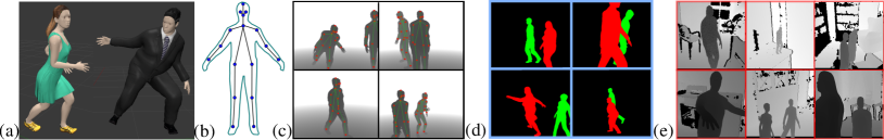
Figure 1: (a) Sample 3D characters with different poses and outfits; (b) skeleton model; (c) rendered synthetic depth image sample; (d) examples of generated colored depth mask for synthetic images with more than one person; (e) examples of training images, combining synthetic generated bodies with real background images.

II-C Model compression and knowledge distillation

Accurate CNN rely in increasingly deeper architectures. Normally, these are over-parameterized and binded with large computational cost, hindering their practical application.

Recent works overcome this over-parametrization by exploring channel pruning [34] or by designing lightweight CNN architectures [8, 9]. On one hand, model pruning remove filters that produce statistically very low activations during the learning process. On the other hand, lightweight architectures designs aim at directly increasing speed by exploiting different convolution strategies. For example, the MobileNet [8] factorizes standard convolutions into depthwise and pointwise convolutions, reducing computation and model size. The SqueezeNet model [9] constrains the number of input feature channels of layers with large kernel size. These architecture designs have made a tremendous gain towards efficiency, with some of them being able to run 50 times faster than their deeper counterpart with small loss in performance.

Another line of research that pursues the same goal is knowledge distillation [10, 35, 36, 37]. Its objective is to train a small and light CNN, called the student model to mimic a more complex and accurate model named the teacher. The pioneering work in [10] showed how the student model can acquire the teacher knowledge using the teacher activations as soft targets. To boost the student’s generalization capabilities, recent works [35] have proposed to introduce ”hints” as an attempt to additionally mimic the activations of a given hidden layer of the teacher. Matching the teacher and student Jacobians of the learning objective has also been used during distillation [36] and can be seen as a form of data augmentation with Gaussian noise. In [37] knowledge distillation is applied to learn an efficient model for multi-object detection and bounding box regression. The approach exploits the teacher output as an upper bound and apply penalty only when the desired output is below a certain margin.

A novelty of our work is to apply knowledge distillation for body landmark detection and a regression task. In doing so, we strongly couple distillation with the process of refining body landmark predictions and show this improves the performance of our efficient architectures compared to simpler knowledge distillation or learning with hints.

III Depth Image Datasets

In this section we introduce the datasets of depth images we used for training and testing. We start by describing the methodology used to generate our synthetic image dataset. Then, we describe the dataset of real depth images collected with a Kinect 2 sensor.

III-A Synthetic depth images dataset

The appropriate training of CNNs requires large amounts of data with high quality ground truth. Unfortunately, building datasets of humans with annotated body landmarks at large scale can be very expensive. We overcome this by relying on computer graphics and considering the DIH synthetic depth image database introduced in [16]. The dataset contains images displaying single and two people instances with different body pose and view perspectives.

The synthetic dataset was generated by a randomized rendering pipeline. We used real motion capture data (mocap) to perform motion retargeting to a 3D character and applied variations in viewpoints to generate synthetic images with body landmark ground truth. The challenge is how to automatically introduce variability in human shapes, body pose and view point configurations. This is detailed below.

Dataset and annotations. The dataset contains 264,432 images of people performing different types of motion under different viewpoints with 71,711 images displaying two people. Some examples are shown in Figure 1(c). The body skeleton comprises 17 body landmarks as shown in Figure 1(b). The landmarks, i.e. head, neck, shoulders, elbows, wrists, hips, knees, ankles, eyes, are extracted in 3D camera and 2D image coordinates. The dataset also provides keypoint visibility and color labeled silhouette masks which can be used to determine keypoint visibility and to perform data transformations during training like adding pixel noise or fusing with real backgrounds (see below). See Figure 1(d) for some examples.

Variability in body shapes. We rely on a dataset of 24 3D characters that show variation in gender, heights and weights, and were dressed with different clothing outfits to increase shape variations (skirts, coats, pullovers, etc.). See Figure 1(a).

Synthesis with two people instances. Multi-person pose estimation scenarios are covered by adding two 3D characters to the rendering scene. During synthesis, two models are randomly selected from the character database and placed randomly in the virtual scene, but keeping a minimum distance between them to avoid checking for collision.

Variability in body poses. Motion simulation is used to add variability in body pose configurations. We performed motion retargeting from motion capture data sequences taken from the CMU Mocap dataset [38]. Amongst the available actions, we selected the following ones as most representative of our target scenario: walking, jogging, jumping, stretching, turning and various sport gesturing.

Variability in view point. A camera is randomly positioned at a maximum distance of 8 meters from the models, and randomly oriented towards the models torso.

Real background fusion. A solution would be to generate random background content by randomly placing 3D objects in the rendering pipeline. This is however non-trivial as a large variety of objects is needed to cover all expected backgrounds. For this reason, in this paper we propose instead to use background images from the target depth sensors. This has 2 main advantages. First, a large variety of background scenes with different contents can easily be collected. Second, the resulting data will already contain sensor specific information that will aid in the generalization capabilities of the learned models. In practice, background generation is performed on the fly during training by fusing the real background image content with the synthetic depth images with people. Some example images are shown in Figure 1(e). Section VII-A1 describes this process in detail.

Body landmark visibility labels. We provide visibility labels for each of the body landmarks in the image. The visibility labels account for partial and self occlusions. A body landmark is set to visible by thresholding the distance between the landmark and the body surface point that projects onto the image at the same position than the landmark.

III-B Real depth image dataset

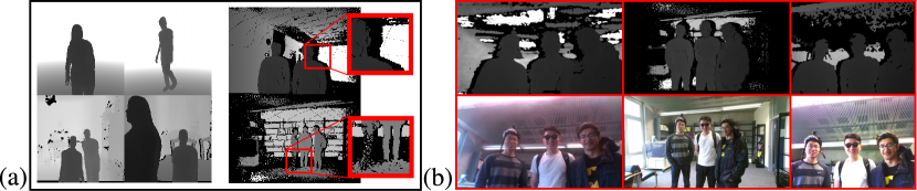
Figure 2: Depth imaging characteristics. (a) some visual characteristics of real depth images (right) like shadows around the silhouette or sensing failures due to surface material and depth variation (red square) are difficult to synthesize and therefore not present in the synthetic images (left); (b) HRI scene recorded with different RGB-D cameras. Left to right: Intel D435, Kinect 2 and Asus Xtion. Different depth sensors have different quality characteristics.

Depth imaging is usually the result of a triangulation process in which a series of laser beams are cast into the scene, captured by an infrared camera, and correlated with a reference pattern to produce disparity images and finally the distance to the sensor. As a result, the image quality greatly depends on the sensor specifications like measurement variance, missing data, surface discontinuities, etc. Samples from three different sensors are shown in Figure 2(b). In particular, sensor limitations such as shadows around the silhouette or sensing failures due to surface material and depth variations are not present in the synthetic images since they are difficult to realistically simulate. As a result and as illustrated in Figure 2(a), there exists a large difference in the visual features exhibited by synthetic and real depth images.

In this paper we relied on data from the Kinect 2 sensor. Compared to other sensors like Intel D435 or Asus Xtion, it has a more accurate depth estimation and a large field of view which is better for HRI analysis. We consider the real data fold of the DIH dataset. It contains 16 indoor sequences of up to three minutes composed of pairs of registered color and depth images. They display up to three people captured at different distance from the sensor and with different levels of occlusion and scene backgrounds. A total of 9 different participants were involved in natural HRI interaction situations (walking off and towards the robot, stretching hands and between person interactions). They wore different clothing accessories to add variability in body shape.

IV Efficient human pose estimation

This section describes the efficient CNN models we investigated for the task of body landmark localization and pose estimation. We start by introducing the pose machine architecture which forms the base of all our models. Then, we present the different instantiations that we investigated to improve efficiency while maintaining accuracy.

IV-A Pose machines CNN architecture class

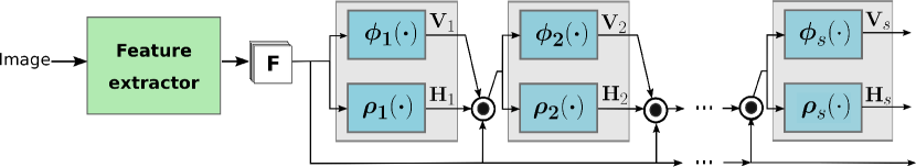
Figure 3: Pose machine architecture class. It comprises a feature extractor module and a prediction cascade. Each stage in the prediction cascade is composed by two branches that predict confidence maps of body landmarks and body limbs in the image. They take as input the extracted features $\mathbf{\mathbf{F}}$ and the confidence maps from the previous stage to refine predictions.

The pose machine architecture comprises two main components: a feature extractor module and a cascade of predictors that output confidence maps for each of the body landmarks and body limbs. Figure 3 sketches the architecture class concept and its main components.

More precisely, the CNN takes an image as input and the feature extractor module computes an abstract representation of it composed of $N_{w}$ channels, denoted as $\mathbf{F}$. These features $\mathbf{F}$ are passed to the cascade of predictors, composed of a series of prediction stages sequentially stacked. Each prediction stage aims at localizing body landmarks (neck, elbows, ankles) and limbs, which are segments between two landmarks according to the skeleton shown in Figure 1 (forearms or thighs).

Each stage $s$ consists of two branches made of fully convolutional layers predicting confidence maps of body landmarks, denoted $\rho_{s}(\cdot)$, and of body limbs, denoted $\phi_{s}(\cdot)$. For $s\geq 2$ these branches take as input both the features $\mathbf{F}$ and the landmark and limbs predictions maps from stage $s-1$. In effect, this allows the refinement of the predictions of each element (landmark and limbs) by incorporating context from the other body parts and hence accounting for valid body pose configurations. This effectively reduces the number of pairs of detected body landmarks and potentially connected, easing the single and multi-person pose inference stage.

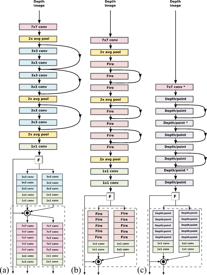
Figure 4: Architecture instances of the pose machines class. (a) Residual pose machines focuses on speeding up the feature extractor module using ResNet modules; (b) SqueezeNet pose machines builds on the Fire module concept to design a lighter architectures; (c) MobileNet pose machines relies on depthwise and pointwise convolution layers to speed up computation. Convolution layers marked with * have a stride of 2 and serve as pooling mechanism.

IV-B Efficient pose machines

For an efficient forward pass, instances of the above architecture class will incorporate lightweight designs in the feature extractor, $\rho_{s}(\cdot)$ and $\phi_{s}(\cdot)$. In Figure 4 we illustrate the design of our efficient pose machine instances. Modules enclosed by doted squares are the components which are replicated to achieve the cascade of predictors. We describe these architectures in the following.

IV-B1 Residual pose machines

In the pose machine architecture instance presented in [5], the first computational bottleneck is the large VGG-19 architecture used as feature extractor module. Therefore, we propose to investigate how to exploit a lighter module built upon residual modules (or blocks) [7]. We originally introduced this modification in [15]. Our motivation is that residual blocks are known to outperform VGG networks, and to be faster by having a lower computational cost [39]. Figure 4(a) depicts the architecture we dubbed as residual pose machines.

Feature extraction network. It consists of an initial convolutional layer followed by three residual modules with small kernel sizes (${3\times 3}$). The network has three average pooling layers. Each residual module consists of two convolutional layers and a shortcut connection. Batch normalization and ReLU are included after all convolutional layers and shortcut connections as exemplified in Figure 5(a).

Pose regression cascade. We maintain a large effective receptive field in the design of the branches $\phi_{s}(\cdot)$ and $\rho_{s}(\cdot)$. In the first prediction stage the network has three convolutional layers with filters of ${3\times 3}$ and two layers with filters of ${1\times 1}$, whereas in the remaining stages there are five and two convolutional layers with filters of ${7\times 7}$ and ${1\times 1}$ respectively.

IV-B2 Squeezenet pose machines

In [9] the SqueezeNet architecture is build upon a series of modules called Fire modules. Each module is composed by a squeeze layer and an expand layer. The squeeze layer contains filters of $1\times 1$ and outputs $N_{s_{1}}$ channels, while the expand layer is a mix of filters of ${1\times 1}$ and ${3\times 3}$ that outputs $N_{e_{1}}$ and $N_{e_{3}}$ channels respectively. This configuration aims to reduce the model size by using $1\times 1$ filters, and to speed up computation by limiting the number of input feature channels of the $3\times 3$ layers. Figure 5(b) illustrates the composition of a Fire module.

Our architecture design using Fire modules is shown in Figure 4(b). The output of the Fire module is the concatenation of the channels from the $1\times 1$ and $3\times 3$ expand layers. We follow the original design and set $N_{s_{1}}$ to be less than the sum $N_{e_{1}}+N_{e_{3}}$ and maintain these quantities low. Batch normalization and ReLU are added after each convolution.

Feature extraction network. The feature extractor module comprises 7 Fire modules, three average pooling layers, three residual connections and two $1\times 1$ convolution layers. ReLU activations are included after the shortcut connection following the design in Figure 5(a).

Pose regression cascade. The pose regression cascade employs five Fire modules and two $1\times 1$ convolution layers in the design of both branches $\phi_{s}(\cdot)$ and $\rho_{s}(\cdot)$.

IV-B3 Mobilenet pose machines

MobileNets [8] are built on separate filters factorizing a standard convolution layer into a depthwise and a pointwise convolution layers. A depthwise operation applies a spatial filter to each input channel (one different filter per channel). Pointwise filters are the classical $1\times 1$ convolution filter that performs a linear combination of all channels of the depthwise output. This factorization has a high impact in the size and the computation that the model requires. Figure 5(c) illustrates the design we follow to implement depthwise and pointwise convolution filters. $3\times 3$ filters are used for the depth wise convolutions. We add batch normalization and ReLU units after each convolution.

Feature extraction network. It is composed of 8 depthwise - pointwise layers, denoted as Depth/point in Figure 4(c). Pooling mechanisms are included in the form of convolutions with stride 2 (denoted with *). We also include three residual connections following the design in Figure 5(a).

Pose regression cascade. In each stage, we compose both branches by 5 depthwise-pointwise modules followed by two $1\times 1$ convolution layers.

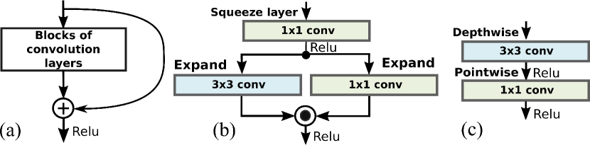
Figure 5: Different unit modules used in our architecture designs. (a) In the residual module we use the sum operation to combine inputs from the shortcut connection and the set of convolution layers; (b) fire modules in SqueezeNets combines $1\times 1$ and $3\times 3$ convolution layers output with a concatenation operation; (c) in MobileNets a standard convolution is decomposed into depthwise and pointwise convolution layers.

IV-C Confidence map ground truth and training

We regress confidence maps for the location of the different body parts and predict vector fields (part affinity fields) for the location and orientation of the body limbs. The ideal representation of the body part confidence maps $\mathbf{H}^{*}$ encodes their locations in the depth image as Gaussian peaks. Let $\mathbf{x}_{j}$ be the ground truth position in the image of body part $j$. The value $\mathbf{H}^{*}_{j}(\mathbf{p})$ for pixel $\mathbf{p}$ in the target confidence map $\mathbf{H}^{*}_{j}$ of the $jth$ part is computed as

$$\mathbf{H}^{*}_{j}(\mathbf{p})=exp\left(-\frac{||\mathbf{p}_{j}-\mathbf{x}_{j}||_{2}^{2}}{\sigma^{2}}\right),$$ (1)

where $\sigma$ is chosen empirically.

Regarding the limbs, the ideal representation $\mathbf{V}^{*}$ encodes with a vector field the confidence that two body parts are associated, as well as the information about the orientation of the limbs. Consider a limb of type $c$ that connects two body parts $j_{1}$ and $j_{2}$ (e.g. elbow and wrist) and their positions on the depth image are $\mathbf{x}_{j_{1}}$ and $\mathbf{x}_{j_{2}}$. The ideal affinity field at point $\mathbf{p}$ is defined as

$$\mathbf{V}_{c}^{*}(\mathbf{p})=\begin{cases}\mathbf{v}&\text{if $\mathbf{p}$ is on limb $c$}\\ 0&\text{otherwise}\end{cases},$$ (2)

where $\mathbf{v}$ is the unit vector that goes from $\mathbf{x}_{j_{1}}$ to $\mathbf{x}_{j_{2}}$. The set of pixels that lie on the limb are those within a distance to the line segment that joins the two body parts.

Training. Supervision is applied at the end of each prediction stage to prevent the network from vanishing gradients. This supervision is implemented by two $L_{2}$ loss functions, one for each of the two branches, between the predictions $\mathbf{H}_{s}$ and $\mathbf{V}_{s}$ and the ideal representations $\mathbf{H}^{*}$ and $\mathbf{V}^{*}$ for stage $s$

$$L_{s}^{\mathbf{V}}=\sum_{\mathbf{p}\in\mathbf{I}}||\mathbf{H}_{s}(\mathbf{p})-\mathbf{H}^{*}(\mathbf{p})||_{2}^{2},$$ (3)

$$L_{s}^{\mathbf{H}}=\sum_{\mathbf{p}\in\mathbf{I}}||\mathbf{V}_{s}(\mathbf{p})-\mathbf{V}^{*}(\mathbf{p})||_{2}^{2}.$$ (4)

The final multi-task loss is computed as:

$$L_{PM}=\sum_{s=1}^{S}\left(L_{s}^{\mathbf{H}}+L_{s}^{\mathbf{V}}\right),$$ (5)

where $S$ is the total number of prediction stages.

IV-D Body part association

We use the algorithm presented in [5] that uses the part affinity fields as confidence to associate the different body landmarks and perform the inference of the 2d pose. It works in a greedy fashion exploiting the skeleton tree structure, analyzing pairs of body landmarks that are potentially linked by a limb type and builds the pose estimate increasingly.

In a nutshell, the method takes as input a given limb type, e.g. forearm. All detected body landmarks that form such limb type (wrists and elbows) are connected one to one, forming potential limbs. The connections are weighted by averaging the predicted vector field along the line that joins the pair of body landmarks. Connections with high confidence are kept while the other discarded. Final pose estimates are built by associating the limb candidates (forearm and arm) that share body landmark candidates (shoulder, elbow and wrist).

V Adversarial Domain Adaptation

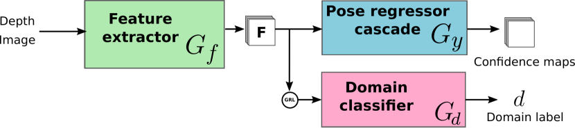
Figure 6: Architecture used for domain adaptation. The base architecture is composed of a feature extractor module $G_{f}$ and a pose regression cascade $G_{y}$ (as in Figure 3). It is extended with a domain classifier $G_{d}$ for depth domain adaptation.

We are given a source sample set (synthetic depth images) $\mathcal{S}=\{(\mathbf{I}_{i},\mathbf{x}_{i})\}_{i=1}^{N}$ and a target dataset (real depth images) $\mathcal{T}=\{\mathbf{I}_{i}\}_{i=1}^{M}$. Note that we are only given annotations of 2d keypoint locations $\mathbf{x}_{i}$ for the source samples $\mathbf{I}_{i}$. The goal is to learn a human pose predictor using the sample $\mathcal{S}$ which performs well on data from $\mathcal{T}$, by mapping source and target data to an invariant representation. We follow the approach in [30] in which more information can be found.

The distance between the source and target distributions of the input data can be measured via the H-divergence. As it is impractical to compute, it can be approximated by considering the generalization error of a domain classification problem. In essence, the distance will be minimum if a domain classifier is incapable of distinguishing between the samples from the different domains. Such domain confusion can be achieved by learning a mapping from the input data to an image representation invariant across domains.

To do so, we rely on the architecture presented in Figure 6. It is a multi-task architecture comprising three main components. The first one, $G_{f}$ with parameters $\theta_{f}$ extracts features from the input image. Sharing these features, the branch $G_{y}$ with parameters $\theta_{y}$ detects body landmarks and limbs in the image. In parallel the branch $G_{d}$ with parameters $\theta_{d}$ classifies the input image into a domain label $d\in\{synthetic,real\}$. The adversarial adaptation procedure consists of learning a $G_{f}$ network able to produce high level features sufficient for body landmark detection but which fool the domain classifier $G_{d}$.

More formally, let us denote by $\mathbf{F}_{\mathbf{I}}$ the internal representation of image $\mathbf{I}$ in the network (features), which is computed as $\mathbf{F}_{\mathbf{I}}=G_{f}(\mathbf{I};\theta_{f})$. We can then define as a measure of domain adaptation the opposite of the standard cross-entropy loss for the domain classifier

$$L_{d}(\theta_{f},\theta_{d})=-\frac{1}{N+M}\sum_{\mathbf{I}\in\mathcal{T}\cup\mathcal{S}}l_{d}(G_{d}(\mathbf{F}_{\mathbf{I}};\theta_{d}),I_{d}),$$ (6)

where $l_{d}$ is a logistic regression loss and $I_{d}$ is the domain label associated with image $\mathbf{I}$. $G_{d}$ is a domain classifier such that $G_{d}(\mathbf{F}_{\mathbf{I}};\theta_{d})=1$ if $\mathbf{I}$ is a real depth image and 0 otherwise. Optimizing the domain classifier is achieved by maximizing

$$R_{d}=\max_{\theta_{d}}L_{d}(\theta_{f},\theta_{d}).$$ (7)

As shown in [30], Eq (7) approximates the empirical H-divergence, measuring the similarity of the real and synthetic samples through the learned features $\mathbf{F}_{\mathbf{I}}$. Such similarity measure can then be combined with the regression loss to define our adversarial loss:

$$L_{DA}(\theta_{f},\theta_{y},\theta_{d})=L_{PM}(\theta_{f},\theta_{y})+\lambda\max_{\theta_{d}}L_{d}(\theta_{f},\theta_{d}),$$ (8)

where $\lambda$ represents the trade-off between landmark localization and domain adaptation, and $L_{PM}(\cdot)$ is defined by Eq. (5).

The adversarial learning process then consists of finding the optimal saddle point of the ’min-max’ loss in Eq (8) by alternating the optimization of the parameters of the body landmark detector through the minimization $(\hat{\theta_{f}},\hat{\theta_{y}})=\arg\min_{\theta_{f},\theta_{y}}L_{DA}(\cdot,\hat{\theta_{d}})$, and the maximization $\hat{\theta_{d}}=\arg\max_{\theta_{d}}L_{DA}(\hat{\theta_{f}},\hat{\theta_{y}},\theta_{d})$. Therefore, $\theta_{f}$ evolves adversarially to increase the domain classification confusion while minimizing the error for landmark detection.

In practice we implemented the domain classifier using a network composed of two average pooling layers with an intermediate layer of $1\times 1$ convolution, and two fully connected layers before the classification sigmoid function at the end. We followed [30] and included a gradient reversal layer (GRL) in the architecture to facilitate the joint optimization of Eq (8). The GRL acts as identity function during the forward pass of the network, but reverses the direction of the gradients from the domain classifier during backpropagation.

Due to the difference in nature between the pose regression and domain adaptation problems, their losess involved in Eq (8) span different ranges. Therefore, the trade-off parameter $\lambda$ has to reflect both the importance of the domain classification as well as to this difference between ranges. Its setting is detailed in Section VII-F.

VI Distilling the pose from a network

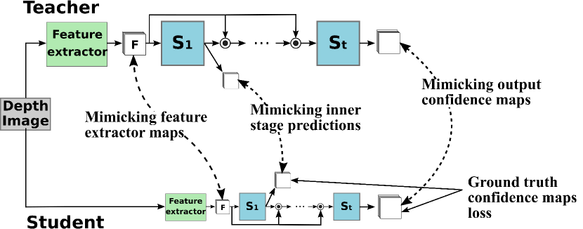
Figure 7: Proposed knowledge distillation scheme for body landmark detection in a cascade of detectors fashion. The student is trained to mimic (in addition to ground truth) the confidence map predictions of body landmarks and body limbs from a pre-trained and robust teacher at the different stages in the cascade of regressors. We additionally adopt the learning by hints approach by encouraging the features of student to match those of the teacher.

Training a CNN model usually relies on data with ground truth. However, the data samples are often of different complexity levels. Intuitively, factors like the camera view point, the pose configuration, the occlusion level (whether due to external elements or to its own body), clothing or object artefacts will render the landmark prediction more or less difficult, an element which is not reflected in the ground truth. While large over-parametrized networks, when supplied with enough data, can usually accommodate this diversity during training, smaller more efficient networks, by attempting to satisfy the ground truth of all data equivalently, can be more easily trapped in local minima with limited generalization. Several methods have been proposed to improve training. One of them is curriculum learning [40], i.e. starting from easier to more complex data samples. Another direction is knowledge distillation that we now introduce.

The distillation approach can be posed as follows: given a deep and large teacher network $T_{net}$, we would like to improve the generalization ability of an efficient student $S_{net}$ using the ”knowledge” acquired by $T_{net}$. Such knowledge transfer can be of several forms. First, it usually involves mimicking the output activations of the teacher as these activations implicitly contains information about the difficulty of the samples (e.g. ambiguity between classes, uncertainty due to difficult imaging conditions). However, it can also include mimicking some of the hidden layers activation maps. In this case, the activations are referred as hints and the goal is to drive the student learning towards learning intermediate representations thought as important from a design process.

We learn accurate and efficient models by using a teacher with high performance using the distillation strategy illustrated in Figure 7. We have investigated several configurations. First, performing distillation at every stage on the cascade of the teacher, i.e. matching the predictions of the teacher at every prediction stage in the cascade to distil the knowledge at every prediction stage and to promote an early on semantic knowledge distillation. Note that this contrasts with the conventional distillation approach which considers only the final prediction as knowledge to transfer. Second, adopting distillation by hints to encourage the student to learn a data representation similar to that of the teacher. These two approaches can be combined in an overall pose distillation objective written as follows:

$$L_{distil}=L_{stages}+\gamma L_{hints}.$$ (9)

The $L_{stages}$ and $L_{hints}$ losses are described below.

VI-A Mimicking teacher stage predictions

We couple knowledge distillation with our architecture designs and perform distillation at the last prediction stages of the cascade. The motivation is that the teacher’s predictions in these last stages contain valuable information about how the teacher refines predictions, which may help the student on how to increasingly improve its own predictions. In practice, we use a weighted sum of losses considering the teacher’s predictions and the ground truth $L_{PM}$ which also introduces information that the student should mimic:

$$L_{stages}=(1-\alpha)L_{teacher}+\alpha L_{PM},$$ (10)

where $L_{PM}$ is defined in Eq (5) and $\alpha$ is a weighting parameter set to 0.5 in our experiments. We choose to model $L_{teacher}$ as to match the prediction of the $\tau$ ($\tau\geq 1$) last stages of the cascade. $L_{teacher}$ is defined as

$$L_{teacher}=\sum_{s=0}^{\tau-1}\left(L^{\mathbf{H}}_{S-s}+L^{\mathbf{V}}_{S-s}\right),$$ (11)

where $S$ is the number of prediction stages in the teacher’s cascade, and

$$L^{\mathbf{H}}_{s}=\sum_{\mathbf{p}\in\mathbf{I}}||\mathbf{H}_{s}(\mathbf{p})-\mathbf{H}^{tea}_{s}(\mathbf{p})||_{2}^{2},$$ (12)

$$L^{\mathbf{V}}_{s}=\sum_{\mathbf{p}\in\mathbf{I}}||\mathbf{V}_{s}(\mathbf{p})-\mathbf{V}^{tea}_{s}(\mathbf{p})||_{2}^{2},$$ (13)

where $\mathbf{p}$ is a pixel in image $\mathbf{I}$, and $(\mathbf{H}^{tea}_{s},\mathbf{V}^{tea}_{s})$ are the body part and part affinity fields confidence maps at stage $s$ of the teacher. Notice that the number of stages in the teacher and student prediction cascades need to be at least $\tau$.

VI-B Learning with hints

We consider this approach by enforcing similarities between the feature extractor outputs in the teacher and student architectures, as it is a natural choice in our architecture designs. Note that our formulation in Eq (11) is a form of distillation with hints for $\tau>1$.

Thus, denoting by $\mathbf{F}^{tea}_{\mathbf{I}}$ the internal representation of image $\mathbf{I}$ of the teacher, we define the hints loss as

$$L_{hints}=||\mathbf{F}_{\mathbf{I}}-\mathbf{F}^{tea}_{\mathbf{I}}||_{2}^{2},$$ (14)

Note that when performing knowledge distillation with hints it is necessary to tie the dimensions of $\mathbf{F}_{\mathbf{I}}$ and $\mathbf{F}^{tea}_{\mathbf{I}}$.

VII Experiments and Results

In this section we describe the experiments we performed to evaluate our approaches. The experimental protocol focuses on both accuracy and computational aspects. We first evaluate the proposed efficient CNN architectures and the impact of the synthetic dataset for training. Then we report on the application of the adversarial domain adaptation approach and its limitations. Finally, we analyze our approach for knowledge distillation and its benefits in our context.

VII-A Data

As data, we considered the synthetic and real parts of the publicly available DIH dataset introduced in Section III, as well as a subset of the CMU-Panoptic dataset, which we briefly describe below. With both synthetic and real images, we performed data augmentation during training: rotation by a random angle within $[-20,20]$ degrees with a 0.8 probability, and image cropping to the $368\times 368$ training size with a probability of 0.9. Unless stated otherwise, we use DIH-Real as our default (real) dataset in the result section.

VII-A1 Synthetic data

Train, validation and testing folds contain 230934, 22333 and 11165 synthetic depth images respectively. To avoid our pose detector to overfit clean synthetic image details, we propose to add image perturbation, in particular, adding real background content which will provide the network with real sensor noise.

Adding real background content. Obtaining real background depth images (which do not require ground-truth) is easier than generating synthetic body images. As background images, we consider the dataset in [41] containing 1367 real depth images recorded with a Kinect 1 and exhibiting depth indoor clutter, and we divided it into training, validation and test folds. In the training case, images were produced on the fly by randomly selecting one depth image background and body synthetic images, and generating a depth image using the character silhouette mask. We simply verified that there was a sufficient depth margin between the body foreground and the background, adding if necessary an adequate depth constant value to the entire background image. While crude, this approach resulted in more realistic data than the synthetic ones. Sample results are shown in Fig. 1(e).

Pixel noise. During training we randomly selected 20% of the body silhouette’s pixels and set their value to zero.

VII-A2 Real data

We consider the following datasets.

DIH-Real. It consists of 16 sequences divided into train, validation and testing folds comprising 7, 5 and 4 sequences respectively. We manually annotated a small subset of images for each fold: 1750, 750 and 1000 images within the training, validation, and testing folds, respectively.

Panoptic. We used a subset of the large CMU-Panoptic dataset [42] from the Range of Motion (RM) and Haggling (H) scenarios (specifically, RM:171204 pose3 and H:170407 haggling a3 for training, RM:171204 pose5 and H:170407 haggling b3 for testing). To be consistent with our experimental setting, where few labeled data are available, we randomly considered 2K images for training and 1K for testing.

VII-B Evaluation metrics

Pose estimation performance. We use standard precision and recall measures derived from the Percentage of Correct Keypoints (PCK) evaluation protocol as performance metrics [17]. More precisely, after the forward pass of the network, we extract all the landmark predictions $p$ whose confidence are above a threshold $\eta$, and run the part association algorithm to generate pose estimates from these predictions. Then, for each landmark type, and for each ground truth points $q$, we associate the closest prediction $p$ (if any) whose distance to $q$ is within a distance threshold $d=\kappa\times h$, where $h$ stands for the height of the bounding box of the person (in the ground truth) to which $q$ belongs to. Such associated $p$ are then counted as true positives, whereas the rest of the landmark predictions are counted as false positives. Ground truth points $q$ with no associated prediction are counted as false negatives. Recall and precision values are computed for each landmark type counting true positives, false positives and false negatives over the dataset. Finally, the average recall (AR) and average precision (AP) values used to report performance are computed by averaging the above recall and precision over landmark type and over several distance thresholds $d$ by varying $\kappa\in[0.05,0.15]$.

Computational performance. Model complexity is measured via the number of parameters it comprises, and the number of frames per second (FPS) it can process when considering only the forward pass of the network. This was measured using the median time to process 2K images at resolution $444\times 368$ pixels with an Nvidia card GeForce GTX 1050.

VII-C Implementation details

Image preprocessing. The depth images are normalized by scaling linearly the depth values in the $[0,8]$ meter range into the $[-0.5,0.5]$ range.

Network training. Pytorch is used in all our experiments. We train different network architectures with stochastic gradient descent with the momentum set to 0.9, the decay constant to ${5\times 10^{-4}}$, and the batch size to 10. We uniformly sample values in the range $[4\times 10^{-10},4\times 10^{-5}]$ as starting learning rate and decrease it by a factor of 10 when the validation loss has settled. All networks are trained from scratch and progressively, i.e. to train network architectures with $s$ stages, we initialize the network with the parameters of the trained network with ${s-1}$ stages. Unless otherwise stated, each model was trained with synthetic data for 13 epochs and finetuned with real images for 100 epochs.

Tested models and notation. Residual, mobile and squeeze pose machines are referred to as RPM, MPM and SPM respectively. We set $N_{w}=64$ (number of features) as the default value and we specify when it changes. We add a postfix to specify the number of stages that a model comprises. For example, RPM-2S is the residual pose machine configuration with 2 prediction stages in the cascade of predictors.

VII-D Performance-efficiency trade-off

DIH
					All body			Upper body
Architecture	# Stages	# Features	# Parameters	FPS	AP	AR	F-Score	AP	AR	F-Score
HG [2]	2	-	12.93 M	8.7	84.62	86.26	0.85	86.45	93.70	0.90
CPM-1S [5]	1	128	8.38 M	18.6	92.10	86.44	0.89	96.12	94.99	0.95
CPM-2S [5]	2	128	17.07 M	11.2	94.03	88.96	0.91	96.36	94.98	0.96
RPM-1S	1	64	0.51 M	56.7	90.86	72.07	0.80	94.28	87.77	0.91
RPM-2S	2	64	2.84 M	35.2	94.84	86.41	0.90	96.39	93.91	0.95
RPM-3S	3	64	5.17 M	20.8	93.96	87.72	0.91	97.26	94.72	0.97
RPM-2S	2	128	10.5 M	12.5	93.52	86.07	0.90	95.95	94.02	0.95
MPM-1S	1	64	99.8 K	134.4	88.52	71.36	0.79	92.88	84.74	0.89
MPM-2S	2	64	168.2 K	112.3	92.56	78.63	0.85	94.97	89.92	0.92
MPM-3S	3	64	236.5 K	95.8	92.40	82.79	0.87	95.23	92.36	0.94
MPM-4S	4	64	304.9 K	84.3	91.27	84.06	0.88	95.27	91.87	0.94
SPM-1S	1	64	308.8 K	70.6	89.64	61.58	0.73	93.18	71.38	0.81
SPM-2S	2	64	455.9 K	60.6	91.78	81.68	0.86	95.82	91.47	0.94
SPM-3S	3	64	660.0 K	53.3	92.63	81.98	0.87	96.43	90.84	0.94
SPM-4S	4	64	921.0 K	47.2	93.13	81.36	0.87	96.30	90.58	0.93
Panoptic
					All body			Upper body
Architecture	# Stages	# Features	# Parameters	FPS	AP	AR	F-Score	AP	AR	F-Score
HG [2]	2	-	12.93 M	8.7	85.14	91.06	0.88	86.0	91.0	0.88
CPM-2S [5]	2	128	17.07 M	11.2	96.73	91.66	0.94	96.75	92.07	0.94
RPM-3S	3	64	5.17 M	20.8	97.42	91.48	0.94	97.43	91.48	0.94
MPM-4S	4	64	304.9 K	84.3	96.43	89.17	0.92	97.0	89.06	0.93
SPM-3S	3	64	660.0 K	53.3	95.44	89.24	0.92	96.30	90.35	0.93

TABLE I: Performance (%) on the test set of real depth images and architecture components for the different tested pose machines instances. Upper body comprises only head, neck, shoulders, elbows and wrists.

Table I compares the performance of our proposed architecture configurations. We report both the average recall and average precision for all landmark types in the skeleton model and for the upper body, i.e. head, neck, shoulders, elbows and wrists since upper body detection might be sufficient for any given applications (e.g. HRI). We compare the models’ performance with the F-Score metric (harmonic mean of recall and precision). The table also compares the FPS and the number of trainable parameters of the different architectures.

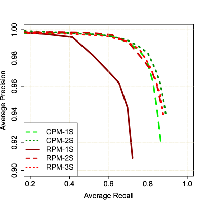
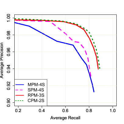
Figure 8: Precision-recall curves obtained by varying the landmark detection threshold $\eta$. Left: comparison between the baseline CPM and the RPM model with different number of prediction stages. Right: performance comparison of our pose machines instances in their deepest version.

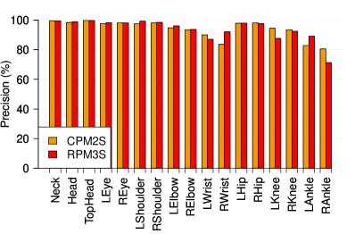
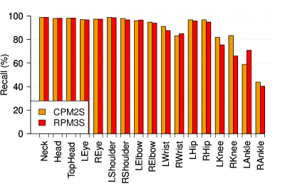
Figure 9: Precision (left) and recall (right) per body landmark for the RPM-3S and the baseline CPM-2S.

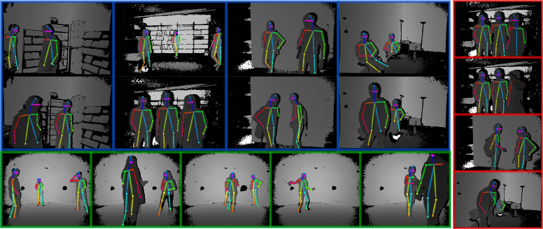
Figure 10: Left: Pose estimation examples from the RPM-3S landmark detector on the DIH dataset (blue squares) and CMU-Panoptic dataset (green squares). Right: Examples of failures cases. They often occur for specific pose or clothings or under occlusion of people or objects (e.g. bags).

VII-D1 Comparison with the Convolutional Pose Machine (CPM) baseline

We consider the CPM architecture presented in [5] as the main baseline. As in the original work, the architecture parameters in the feature extractor module were initialized using the first 10 layers of the VGG-19 network. Parameters in the cascade of detectors were trained from scratch. To accommodate the need for the 3 channel image input expected by VGG-19, the single depth channel is repeated three times. We report the results for architectures comprising up to two stages in the prediction cascade since no substantial performance increase was obtained after the second stage.

We train RPM network architectures with 1, 2 and 3 stages. Figure 8(a) shows the precision-recall curves over the testing set of real depth images, obtained by varying the landmark detection threshold $\eta$. We summarize these curves in Table I taking the performance with the highest F-Score. As can be seen, our RPM models perform as well as the baseline but is lighter and faster. This is specially the case for RPM-2S that shows similar performance as CPM-2S but comprises 6 times less parameters and is 3.14 times faster. Interestingly, we can notice from Figure 8(a) that the smaller complexity of the feature extractor of RPM-1S leads to degraded performance compared to the baseline CPM-1S. This gap is filled once context is introduced with the second stage (see RPM-2S and CPM-2S curves). Adding an extra stage (RPM-3S) slightly improves the model performance while still being faster than the baseline. In particular for the upper body parts where it now slightly outperforms the baseline. Figure 9 compares the per body landmark precision and accuracy for RPM-3S and CPM-2S models, where we can notice very high performance achieved for the upper body landmarks.

Number of feature channels. We set $N_{w}=128$ and train the RPM models. We report the results for RPM-2S with this configuration in Table I. Note how the results of the RPM-2S with $N_{w}=64$ and RPM-2S with $N_{w}=128$ are very similar showing that more feature channels does not bring more benefits. Given its higher computational complexity setting $N_{w}=64$ is a good accuracy-speed trade-off.

Qualitative analysis. Figure 10 shows examples of the pose estimation algorithm using the body landmarks and limbs output of our RPM-2S model. Note that our model is capable of producing strong confidence maps that produce accurate estimates even for the eyes and in the presence of self and person occlusions, profile views, and different body pose configurations and silhouette shapes. The main challenges for our model include strong changes in the person silhouette (backpacks, big jackets) and person proximity and occlusions as illustrated by failure cases in Figure 10(b).

VII-D2 Efficient pose machines

The performance of the MPM and SPM models are presented in Table I. We can first notice that they are more efficient in terms of FPS and number of trainable parameters than the CPM and RPM models. For example, MPM-4S contains 55.9 times less parameters than CPM-2S model and is 7.5 times faster with only a decrease of 0.03 in F-Score. SPM-4S, on the other hand is 4.2 times faster than CPM-2S with a decrease of 0.04 in F-Score.

We note that increasing the number of prediction stages improves the models’ F-Score. As with the RPM models, we observe that the biggest improvement appears when introducing a second stage. The additional stages help refining prediction, for instance by greatly improving the landmark detection recall while the precision saturates or slightly degrades (compare the MPM-2S and MPM-4S results), but in general the results often start saturating after the 3rd stage.

Figure 8(b) illustrates the precision-recall curves for the deepest version of our efficient models. Among the architectures we investigate, the fastest are the MPM designs, followed by SPM models. Nevertheless, the best speed-accuracy trade-off are given by the RPM-2S model when the focus is on accuracy, and MPM-4S when it is on speed.

VII-D3 Comparison with state-of-the-art methods

In addition to the CPM baseline, we compared our methods with the stacked Hourglass framework [2]. We used the same network architecture and training protocol (initialization, learning rate, optimizer) proposed by the authors. For a fair comparison we followed our protocol regarding the data, trained the model with synthetic images for 13 epochs and finetuned it with real data for 100 epochs.

Results in Table I show that our efficient architectures outperform this baseline in efficiency and accuracy, on both the DIH and Panoptic datasets. For example, MPM-4S is 9.6 times faster, 42.2 times smaller, with an F-Score of 0.88 (on DIH) compared to 0.85 for the Hourglass network.

VII-D4 Experiments with CMU-Panoptic dataset

The results on this dataset are shown in Table I (bottom part). We report only the results obtained by the best performing models on the DIH-Real dataset. Our proposed RPM-3S outperforms the Hourglass baseline. It also performs similarly than the CPM baseline. The proposed efficient architectures MPM-4S and SPM-3S outperform the Hourglass baseline by a margin of 0.04 in the F-Score and follow closely the RPM-3S and baseline CPM-2S with a difference of 0.02 in the F-Score.

VII-E Training with synthetic data analysis

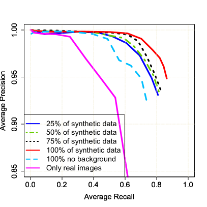
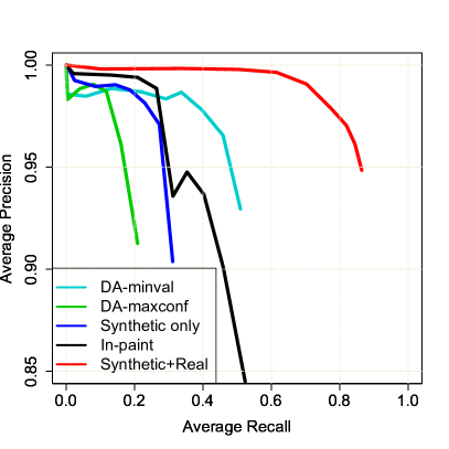
Figure 11: Left: evaluation of the use of synthetic data for learning robust pose estimation models. Right: comparison of different techniques for synthetic-to-real domain adaptation.

We validate the use of the synthetic data to learn accurate models. To this end, we randomly split the synthetic training data in partitions comprising $25\%$, $50\%$, $75\%$ and $100\%$ of it. These partitions contain images with one and two people. We train RPM-2S models with the different synthetic data partitions and then finetune the result with real data. We use the same quantity of labeled data to finetune in all cases (1750 images). Unless otherwise stated, during training we consider all image transformations for data augmentation (background fusion, pixel drop, cropping and rotation). Table II shows the obtained average recall and precision on real data, before and after finetuning. The following conclusions can be made.

	Synthetic only			Synthetic + Finetuning
Synthetic data $\%$	AP	AR	F-Score	AP	AR	F-Score
25 $\%$	94.19	26.28	0.41	93.09	80.83	0.86
50 $\%$	95.10	29.51	0.45	93.45	81.38	0.87
75 $\%$	91.68	30.14	0.45	93.68	82.42	0.88
100 $\%$	90.37	31.14	0.46	93.96	87.72	0.91
100 $\%$ no BG	80.67	3.35	0.06	92.58	73.46	0.82

TABLE II: Comparison of performance obtained with RPM-2S when trained with different synthetic data partitions.

VII-E1 Amount of synthetic data

Performance increases with more synthetic data, both before and after finetuning. Naturally, the visual features mismatch between the synthetic and real data provokes low performance when training only with synthetic data. Nevertheless the gap is covered once finetuning on real data is applied, particularly regarding the recall. Figure 11(a) shows the average precision-recall curves training with the different data partitions and applying finetuning.

VII-E2 Adding realism to synthetic images

We validate our strategy of fusing real background with synthetic depth images to prevent overfiting. To this end, we trained the RPM-2S models with $100\%$ of the synthetic data, helding out the background fusion transformation, and then applied finetuning. We report the results in Table II. Observe that without the addition of real background, our model overfits to the synthetic data details and performs poorly on real data. Interestingly, note as well that even after finetuning on real data the performance is not entirely recovered. The model even performs lower than using only $25\%$ of the synthetic data. Intuitively, fusing background with synthetic images work as a regularizer that prevents overfitting to synthetic image details.

VII-E3 Multiple people data

	All test data			Data with person occlusions
Data fold	AP	AR	F-Score	AP	AR	F-Score
1P-Fold	92.51	80.22	0.86	91.10	82.92	0.87
2P-Fold	92.43	82.44	0.87	93.33	84.81	0.89

TABLE III: Performance obtained with the RPM-2S model when combining synthetic data with only single person images (1P-Fold) and 2 people images (2P-Fold) for training.

We study the importance of having synthetic training images with two people before finetuning with real data. To this end, we define two folds of 100K images for training. The first one (1P-Fold) contains only images with one person; the second one (2p-Fold) contains 50K images with one person and 50K images with two people. The resulting performance is reported in Table III where we also provide results on a test subset where people are very close or occlude each other (see Figure10(b)). The subset contains 211 images with three people where their ground truth bounding boxes overlap between 12.38% and 15.4%. We note that using images with two people helps generalization.

VII-E4 Training with real data only

We train the RPM-2S model only with our small real depth image annotated sample. Figure 11(a) shows the performance curve. Our real dataset sample is not large enough to prevent our model from overfiting and performs worse than using the synthetic data without background fusion.

VII-F Domain adaptation

Adaptation method	CR	AP	AR	F-Score
ADA - Min Loss	0.20	92.95	50.94	0.66
ADA - Max Confusion	0.50	91.26	20.86	0.40
Only synthetic	0.04*	90.37	31.14	0.46
In-paint preprocessing	0.03*	84.49	52.33	0.65
Finetunning	0.15*	93.96	87.72	0.91

TABLE IV: Comparison of performance obtained with the different techniques for domain adaptation using the RPM-2S model. CR stands for the confusion rate obtained in the domain classification task. Values with * were obtained by training a domain classifier using the corresponding model feature extractor as fixed features. In-paint preprocessing corresponds to the application of in-painting before applying the detector.

In these experiments we use the unlabeled training set of real images comprising 4828 Kinect 2 depth images as the target domain. We first train the feature extractor and cascade of predictors of the RPM-2S model with synthetic data for $200K$ iterations. Adversarial domain adaptation (ADA) is then performed by jointly training the domain classifier, feature extractor and cascade of predictors for another $100K$ iterations. Following common practices we gradually updated the trade-off parameter $\lambda$ of eq (8) according to the training progress as $\lambda_{p}=\frac{2\Lambda}{1+exp(-10p)}-\Lambda$, where $p=t/T$, with $t$ the current iteration and $T=100K$. We set $\Lambda=100$ so that the two losses in Eq (8) are in the same range.

VII-F1 Adaptation criteria

During adaptation we monitored validation losses for body landmark detection and domain classification. After $T$ iterations we selected domain adapted models according to two criteria: 1) the minimum of a pose validation loss, and 2) maximum confusion (sum of false positives and false negatives for the domain classification task) on a validation set. Table IV reports the results where we also include the performance of models trained without adaptation.

The adversarial domain adaptation (ADA) framework aims at learning invariant features across domains. Nevertheless, we note that when maximum confusion is achieved the body landmark detection task is greatly hampered, and the model performs even worse than non-adapted models. In contrast, the model selected using a validation error on body landmark detection outperforms the non-adapted models while still achieving some level of domain confusion. We can notice that the recall is greatly affected. Certainly, a major difference between synthetic and real images is the lack of data around external edges that form the limbs extremities and silhouette. These are also the places where pose information is available. Confusing the domain classifier means that features exploiting this lack of data are removed, which hurts the body landmark detection performance.

VII-F2 Inpainting and finetuning methods.

To understand the limits of our unsupervised ADA approach, we compare it with the performance of inpainting and finetuned models. Figure 11(c) shows the precision-recall curves of the different methods, while Table IV summarizes these curves with the maximum F-Score obtained. We see that ADA slightly outperforms the in-painting approach. Indeed, the latter aims to fill the missing depth information as an image preprocessing step for non-adapted models. Observe however that in-painting greatly reduces precision, introducing artifacts in the image that are later confused as body landmarks or limbs. On the other hand, finetuning directly the network initially training on synthetic images with even a small amount of labeled data greatly improves its generalization capabilities.

DIH
Student	Teacher	Distil type	AP	AR	F-Score
CPM-2S	-	-	94.03	88.96	0.91
MPM-2S	-	-	92.56	78.63	0.85
MPM-4S	-	-	91.27	84.06	0.88
MPM-1S	CPM-2S	Stagewise	88.55	71.96	0.79
MPM-1S	CPM-2S	Stagewise + Hints	89.89	76.61	0.83
MPM-2S	CPM-2S	Standard ($\tau=1$)	90.98	80.60	0.85
MPM-2S	CPM-2S	Stagewise	92.10	83.98	0.88
MPM-2S	CPM-2S	Stagewise* ($\tau=2$)	92.42	81.60	0.87
MPM-2S	CPM-2S	Stagewise + Hints	90.91	80.19	0.85
Panoptic
CPM-2S	-	-	96.73	91.66	0.94
MPM-2S	-	-	96.25	86.66	0.91
MPM-4S	-	-	96.43	89.17	0.92
MPM-2S	CPM-2S	Stagewise	95.08	90.33	0.92

TABLE V: Knowledge distillation experiments. Methods with - in the ’Teacher’ and ’Distil type’ fields indicate that the model has been trained without distillation and their values were taken from Table I (i.e. these are the baseline results).

VII-G Pose knowledge distillation

We perform knowledge distillation using CPM-2S as the teacher. We select MPM-1S and MPM-2S models as students given that the MPM design is the most efficient of our pose machines. Our students are trained from scratch. We performed distillation first with synthetic data during 10 epochs, then with real images for 100 epochs. The learning rate is updated in a linear fashion and we set $\gamma$ to 1. Table V reports the results. Our proposed approach of performing distillation at the last stages in cascade is referred to as stagewise. We also experiment by matching only the final activation maps of the teacher at every stage of the student (marked with *).

VII-G1 Knowledge distillation approaches

Our stagewise approach outperforms the same network configurations trained without distillation or with the standard distillation approach (only taking into account the last stage of the cascade). Learning with hints makes the student MPM-1S outperform its stagewise distillation counterpart, but this is not the case with MPM-2S. One possible reason is that given the architecture differences, enforcing feature similarity prevents the student from improving the task loss. In contrast, mimicking the refined predictions at the cascade level using the prediction from the teacher proves to be effective for distillation.

VII-G2 Comparison with baseline models

Knowledge distillation helps boosting the generalization of smaller models. This is particularly true for MPM-2S which with distillation reaches the F-Score performance of its deeper (and slower) version MPM-4S baseline. There is still a small performance gap between the CPM-2S teacher and learner performance (0.03 in F-Score), but the later runs 10 times faster and is 101 times lighter. Interestingly, the same conclusions can be drawn from the distillation results obtained on the CMU-Panoptic dataset, with the MPM-2S improving by 0.1 its F performance using the same distillation approach.

VIII Conclusion

We have investigated and applied different techniques to achieve fast body landmark detection in multi-person pose estimation scenarios. We propose to use depth images in combination with efficient CNN to maintain the trade-off between speed and accuracy. Our approach relies on efficient instantiations of the pose machines with stacked regressors and employing residual modules, SqueezeNets and MobileNets designs. In a set of experiments, we have shown that leveraging on knowledge distillation we can boost the performance of our lightweight models, running at 112.3 FPS with MobileNets with small performance loss. We employ and validate the use of synthetic depth images to cope with the lack of training data and investigated domain adaptation techniques to cope with missing body landmarks in real data. Our study suggest that the fusion of sensor data with synthetic depth images aids the models’ generalization capabilities on real data.

Angel Martínez-González is a research assistant at the Idiap Research Institute and a Ph.D. student at EPFL, Switzerland. He received his M.Sc. in Computer Science from the Mathematical Research Center (CIMAT) in Guanajuato, Mexico. His research interests are machine learning, computer vision and human-computer interaction.

Michael Villamizar is a postodoctoral researcher at the Idiap Research Institute (Switzerland). Before, he was a postdoctoral researcher at the Institut de Robòtica i Informàtica Industrial, CSIC-UPC, in Barcelona (Spain). He obtained his PhD in computer vision and robotics from the Universitat Politècnica de Catalunya in 2012. His research interests are focused on object detection and categorization, robust visual tracking, and real-time robotics applications.

Olivier Canévet is a research and development engineer at the Idiap Research Institute (Switzerland). He received a Ph.D. from the École Polytechnique Fédérale de Lausanne (Switzerland) in 2016 and an engineering degree from TELECOM Bretagne, (France) in 2012. He takes part in various projects related to computer vision and machine learning.

Jean-Marc Odobez (M’03) is the head of the Idiap Perception and Activity Understanding Group and adjunct faculty at the École Polytechnique Fédérale de Lausanne (EPFL). He received his PhD from Rennes University/INRIA in 1994. He is interested in the design of multimodal perception systems for human activity, behavior recognition, human interactions modeling or understanding.

References

- [1] W. Yang, S. Li, W. Ouyang, H. Li, and X. Wang. Learning feature pyramids for human pose estimation. In arXiv:1708.01101, 2017.
- [2] A. Newell, K. Yang, and J. Deng. Stacked hourglass networks for human pose estimation. In European Conf. on Computer Vision, 2016.
- [3] A. Toshev and C. Szegedy. Deeppose: Human pose estimation via deep neural networks. In IEEE CVPR, 2014.
- [4] R. Alp Güler, N. Neverova, and I. Kokkinos. Densepose: Dense human pose estimation in the wild. In IEEE CVPR, 2018.
- [5] Z. Cao, T. Simon, S. Wei, and Y. Sheikh. Realtime multi-person 2d pose estimation using part affinity fields. In IEEE Conf. on Computer Vision and Pattern Recognition (CVPR), 2017.
- [6] J. Shotton, R. Girshick, A. Fitzgibbon, T. Sharp, M. Cook, M. Finocchio, R. Moore, P. Kohli, A. Criminisi, A. Kipman, and A. Blake. Efficient human pose estimation from single depth images. IEEE Transactions on Pattern Analysis and Machine Intelligence, 2012.
- [7] K. He, X. Zhang, S. Ren, and J. Sun. Deep residual learning for image recognition. In Computer Vision and Pattern Recognition (CVPR), 2016.
- [8] A. G. Howard, M. Zhu, B. Chen, D. Kalenichenko, W. Wang, T. Weyand, M. Andreetto, and H. Adam. Mobilenets: Efficient convolutional neural networks for mobile vision applications. In arXiv:1704.04861. 2017.
- [9] F. N. Iandola, S. Han, M. W. Moskewicz, K. Ashraf, W. J. Dally, and K. Keutzer. Squeezenet: Alexnet-level accuracy with 50x fewer parameters and¡ 0.5 mb model size. In arXiv:1602.07360. 2016.
- [10] G. Hinton, O. Vinyals, and J. Dean. Distilling the knowledge in a neural network. In NIPS Deep Learning and Representation Learning Workshop, 2015.
- [11] T. Lin, M. Maire, S. Belongie, J. Hays, P. Perona, D. Ramanan, P. Dollár, and C. L. Zitnick. Microsoft coco: Common objects in context. In European Conf. on Computer Vision (ECCV). 2014.
- [12] Calderara S. Palazzi A. Vezzani R. Cucchiara R. Fabbri M., Lanzi F. Learning to detect and track visible and occluded body joints in a virtual world. In European Conf. on Computer Vision (ECCV), 2018.
- [13] W. Chen, H. Wang, Y. Li, H. Su, Z. Wang, C. Tu, D. Lischinski, D. Cohen-Or, and B. Chen. Synthesizing training images for boosting human 3d pose estimation. In 3D Vision (3DV), 2016.
- [14] C. Lassner, J. Romero, M. Kiefel, F. Bogo, M. J. Black, and P. V. Gehler. Unite the people: Closing the loop between 3d and 2d human representations. In IEEE CVPR, July 2017.
- [15] A. Martínez-González, M. Villamizar, O. Canévet, and J. M. Odobez. Real-time convolutional networks for depth-based human pose estimation. In Int. Conf. on Intelligent Robots and Systems, IROS, 2018.
- [16] A. Martínez-González, M. Villamizar, O. Canévet, and J.M. Odobez. Investigating depth domain adaptation for efficient human pose estimation. In European Conf. of Computer Vision - Workshops, (ECCV), 2018.
- [17] Y. Yang and D. Ramanan. Articulated human detection with flexible mixtures of parts. IEEE Trans. on Pat. Analysis and Machine Intelligence, 2013.
- [18] L. Pishchulin, E. Insafutdinov, S. Tang, B. Andres, M. Andriluka, P. Gehler, and B. Schiele. Deepcut: Joint subset partition and labeling for multi person pose estimation. In IEEE CVPR, 2016.
- [19] E. Insafutdinov, M. Andriluka, L. Pishchulin, S. Tang, E. Levinkov, B. Andres, and B. Schiele. Articulated multi-person tracking in the wild. In Computer Vision and Pattern Recognition (CVPR), 2017.
- [20] U. Iqbal, A. Milan, and J. Gall. Posetrack: Joint multi-person pose estimation and tracking. In IEEE CVPR, 2017.
- [21] J. Carreira, P. Agrawal, K. Fragkiadaki, and J. Malik. Human pose estimation with iterative error feedback. In IEEE Conf. on Computer Vision and Pattern Recognition (CVPR), 2016.
- [22] Z. Wang W. Sun J. Pan J. Liu J. Pang L. Lin Y. Luo, J. Ren. Lstm pose machines. In Computer Vision and Pattern Recognition (CVPR), 2018.
- [23] J. Shotton, A. Fitzgibbon, M. Cook, T. Sharp, M. Finocchio, R. Moore, A. Kipman, and A. Blake. Real-time human pose recognition in parts from single depth images. In IEEE CVPR, 2011.
- [24] H. Y. Jung, S. Lee, Y. Seok Heo, and I. D. Yun. Random tree walk toward instantaneous 3d human pose estimation. In IEEE Conf. on Computer Vision and Pattern Recognition (CVPR), 2015.
- [25] H. Kim, S. Lee, D. Lee, S. Choi, J. Ju, and H. Myung. Real-time human pose estimation and gesture recognition from depth images using superpixels and svm classifier. Sensors, 2015.
- [26] A. Haque, B. Peng, Z. Luo, A. Alahi, S. Yeung, and L. Fei-Fei. Towards viewpoint invariant 3d human pose estimation. In European Conf. on Computer Vision (ECCV), 2016.
- [27] K. Wang, S. Zhai, H. Cheng, X. Liang, and L. Lin. Human pose estimation from depth images via inference embedded multi-task learning. In ACM on Multimedia Conf., 2016.
- [28] G. Moon, J. Chang, and K. M. Lee. V2v-posenet: Voxel-to-voxel prediction network for accurate 3d hand and human pose estimation from a single depth map. In IEEE CVPR, 2018.
- [29] G. Csurka. Domain adaptation for visual applications: A comprehensive survey. In Domain Adaptation in Computer Vision Applications. 2017.
- [30] Y. Ganin, E. Ustinova, H. Ajakan, P. Germain, H. Larochelle, F. Laviolette, M. Marchand, and V. Lempitsky. Domain-adversarial training of neural networks. Journal of Machine Learning Research, 2016.
- [31] M. Long, H. Zhu, J. Wang, and M. I. Jordan. Unsupervised Domain Adaptation with Residual Transfer Networks. In In NIPS. 2016.
- [32] J. Hoffman, E. Tzeng, T. Park, J. Zhu, P. Isola, K. Saenko, A. Efros, and T. Darrell. CyCADA: Cycle-consistent adversarial domain adaptation. In Int. Conf. on Machine Learning (ICML), 2018.
- [33] N. Patricia, F. M. Cariucci, and B. Caputo. Deep depth domain adaptation: A case study. In IEEE Int. Conf. on Computer Vision Workshops, ICCV Workshops, 2017.
- [34] P. Molchanov, S. Tyree, T. Karras, T. Aila, and J. Kautz. Pruning convolutional neural networks for resource efficient inference. In Int. Conf. on Learning Representations, (ICLR), 2017.
- [35] A. Romero, N. Ballas, S. Ebrahimi Kahou, A. Chassang, C. Gatta, and Y. Bengio. Fitnets: Hints for thin deep nets. In In Proceedings of Int. Conf. on Representation Learning (ICRL), 2015.
- [36] S. Srinivas and F. Fleuret. Knowledge transfer with jacobian matching. In Int. Conf. on Machine Learning (ICML), 2018.
- [37] G. Chen, W. Choi, X. Yu, T. Han, and M. Chandraker. Learning efficient object detection models with knowledge distillation. In Advances in Neural Information Processing Systems (NIPS). 2017.
- [38] Cmu motion capture data. http://mocap.cs.cmu.edu/.
- [39] A. Canziani, A. Paszke, and E. Culurciello. An analysis of deep neural network models for practical applications. arXiv:1605.07678, 2016.
- [40] Y. Bengio, J. Louradour, R. Collobert, and J. Weston. Curriculum learning. In Int. Conf. on Machine Learning, 2009.
- [41] P. Kohli N. Silberman, D. Hoiem and R. Fergus. Indoor segmentation and support inference from rgbd images. In European Conf. on Computer Vision (ECCV), 2012.
- [42] H. Joo, T. Simon, X. Li, H. Liu, L. Tan, L. Gui, S. Banerjee, T. Godisart, B. Nabbe, I. Matthews, T. Kanade, S. Nobuhara, and Y. Sheikh. Panoptic studio: A massively multiview system for social interaction capture. IEEE Transactions on Pattern Analysis and Machine Intelligence, 2017.