ReD-CaNe: A Systematic Methodology for Resilience Analysis and Design of Capsule Networks under Approximations

Abstract

Recent advances in Capsule Networks (CapsNets) have shown their superior learning capability, compared to the traditional Convolutional Neural Networks (CNNs). However, the extremely high complexity of CapsNets limits their fast deployment in real-world applications. Moreover, while the resilience of CNNs have been extensively investigated to enable their energy-efficient implementations, the analysis of CapsNets’ resilience is a largely unexplored area, that can provide a strong foundation to investigate techniques to overcome the CapsNets’ complexity challenge.

Following the trend of Approximate Computing to enable energy-efficient designs, we perform an extensive resilience analysis of the CapsNets inference subjected to the approximation errors. Our methodology models the errors arising from the approximate components (like multipliers), and analyze their impact on the classification accuracy of CapsNets. This enables the selection of approximate components based on the resilience of each operation of the CapsNet inference. We modify the TensorFlow framework to simulate the injection of approximation noise (based on the models of the approximate components) at different computational operations of the CapsNet inference. Our results show that the CapsNets are more resilient to the errors injected in the computations that occur during the dynamic routing (the softmax and the update of the coefficients), rather than other stages like convolutions and activation functions. Our analysis is extremely useful towards designing efficient CapsNet hardware accelerators with approximate components. To the best of our knowledge, this is the first proof-of-concept for employing approximations on the specialized CapsNet hardware.

I Introduction

The recently introduced breakthrough concept of Capsule Networks (CapsNets) by the Google Brain team has achieved a significant spotlight due to its powerful new features offering high accuracy and better learning capabilities [25]. Traditional Convolutional Neural Networks (CNNs) are not able to learn the spatial relations in the images much efficiently [25]. Moreover, they make extensive use of the pooling layer to reduce the dimensionality of the space, and consequently as a drawback, the learning capabilities are reduced. Therefore, a huge amount of training data is required to mitigate such deficit. On the other hand, CapsNets take advantage from their novel structure, with so-called capsules and their cross-coupling learnt through the dynamic routing algorithm, to overcome this problem. Capsules produce vector outputs, as opposed to scalar outputs of CNNs [25]. In a vector format, CapsNets are able to learn the spatial relationships between the features. For example, the Google Brain team [25] demonstrated that CNNs recognize an image where the nose is below the mouth as a “face”, while CapsNets do not make such mistake because they have learned the spatial correlations between features (e.g., the nose must appear above the mouth). Other than image classification, CapsNets have been successfully showcased to perform vehicle detection [30], speech recognition [28] and natural language processing [33].

The biggest roadblock in the real-world deployments of CapsNet inference is their extremely high complexity, requiring a specialized hardware architecture (like the recent one in [17]) that may consume a significant amount of energy/power. Not only deep CapsNet models [24], but also shallow models like [25] require intense computations due to matrix multiplications in the capsule processing and the iterative dynamic routing algorithm for learning the cross-coupling between capsules. To deploy CapsNets at the edge, as commonly adopted for the traditional CNNs [4], network compression techniques (like pruning and quantization) [5] can be applied, but at the cost of some accuracy loss. Moreover, the current trends in Approximate Computing can be leveraged to achieve energy-efficient hardware architectures, as well as for enabling design-/run-time energy-quality tradeoffs. However, this requires a comprehensive resilience analysis of CapsNets considering approximation errors in the hardware, in order to make correct design decisions on which computational steps of the CapsNets are more likely to be approximated and which not. Note, unlike in the case of approximations, an error can also be caused by a misfunctioning of the computing hardware [11] or of the memory [12]. Fault injections have demonstrated to fool CNNs [16], and can potentially cause a CapsNet misclassification as well.

Concept Overview and our Novel Contributions:

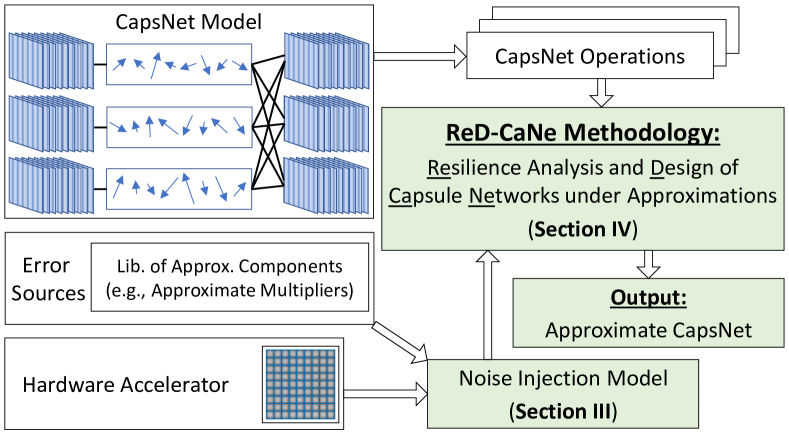
Figure 1: Overview of our ReD-CaNe methodology. The novel contributions are shown in green boxes.

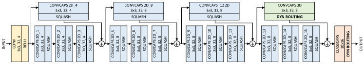
Figure 2: The architecture of the DeepCaps network [24].

To address these challenges, we propose ReD-CaNe, a novel methodology (see Fig. 1) for analyzing the resilience of CapsNets under approximations, which, to the best of our knowledge, is the first of its kind. First, we devise a noise injection model to simulate real-case scenarios of errors coming from approximate hardware components like multipliers, which are very common in multiply-and-accumulate (MAC) operations for the matrix multiplications of capsules. Then, we analyze the error resilience of the CapsNets by building a systematic methodology for injecting noise into different operations of the CapsNet inference, and evaluating their impact on the accuracy. The outcome of such analysis will produce guidelines for designing and selecting approximate components, based on the resilience of each operation. At the output, our methodology produces an approximated version of a given CapsNet, to achieve an energy-efficient inference.

I-A In a nutshell, our novel contributions are:

• We analyze and model the noise injections that can be generated by different approximate arithmetic components, e.g., multipliers. (Section III)

• We devise ReD-CaNe, a novel methodology for analyzing the Resilience and Designing Capsule Networks under approximations, by systematically adding noise at different operations of the CapsNet inference and by monitoring the test accuracy. The approximated components are selected based on the resilience level of the different operations of the CapsNet inference. (Section IV)

• We test our methodology on several benchmarks. On the DeepCaps model [24] for CIFAR-10 [13], MNIST [14], and SVHN [22] datasets, and on the CapsNet model [25] for MNIST and Fashion-MNIST [29] datasets. Our results demonstrate that the least resilient operations are the convolutions in CapsLayers, while the operations performed during the dynamic routing of the Caps3D and ClassCaps layers are relatively more resilient. (Section VI)

Before proceeding to the technical sections, in Section II, we summarize the concepts of CapsNets and review the existing works of error resilience for traditional CNNs, with necessary details to understand the rest of the paper.

II Background and Related Work

II-A Capsule Networks (CapsNets)

CapsNets, first introduced in [9], have become popular in [25], thanks to the new concepts like capsules and the dynamic routing algorithm. Following this trend, DeepCaps [24] proposed to increase the depth of CapsNets, achieving state-of-the-art accuracy for the CIFAR10 [13] dataset.

A capsule is a group of neurons where the instantiation parameters are represented as the orientation of each element of the vector, and the vector length represents the probability that the entity exists. Moreover, vector predictions of the capsules need to be supported by nonlinear vectorized activation functions. Towards this end, the squashing function bounds the output of the capsule between 0 and 1.

In the dynamic routing, the coupling coefficients, which are connecting two consecutive capsule layers, learn the agreement during the inference by iteratively updating their values according to the relevance of the path. As an example, the architecture of the DeepCaps is shown in the Fig. 2. It has 16 convolutional capsule layers (ConvCaps), where one of them is 3D, and one fully-connected capsule layer (ClassCaps) at the end. A special focus is on the operations required for the dynamic routing, which is performed in the 3D ConvCaps and in the ClassCaps layers, as shown in Fig. 3. Note that the operations like matrix-vector multiplications and squash are different from the traditional CNNs. Hence, a challenge that we want to address in this paper is to study the inter-relation between the precision of these operations and the accuracy of the CapsNets, when subjected to errors due to approximations.

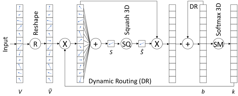
Figure 3: The operations to be computed for the dynamic routing.

II-B Error Resilience of Traditional CNNs

The resilience of traditional CNNs has recently been investigated in the literature. Du et al. [2] analyzed the error resilience, showing that it is possible to obtain high energy savings with minimal accuracy loss. Hanif et al. [7] proposed a methodology to apply approximations for CNNs, based on the error resilience. Li et al. [15] studied the error propagation with the end goal of adopting countermeasures for obtaining resilient hardware accelerators. Zhang et al. [31] proposed a method to design fault tolerant systolic array-based accelerators. Hanif et al. [6] introduced a method for applying approximate multipliers into CNN accelerators without any error in the final result. Mrazek et al. [21][20] proposed a methodology to successfully search and select approximate components for CNN accelerators. Hanif et al. [8] and Marchisio et al. [18] analyzed cross-layer approximations for CNNs. However, these works analyzed only traditional CNN accelerators, and such studies cannot be efficiently extrapolated for CapsNets, as discussed before. Hence, there is a dire need to perform the resilience analysis for CapsNets in a systematic way, such that we can take efficient decisions about approximating the appropriate operations of CapsNets.

II-C Error Sources

In a generic Deep Learning application, errors may occur due to different sources like software approximations (e.g., quantization), hardware approximations (e.g., approximate multipliers), transient faults (i.e., bit flips due to particle strikes) and permanent faults (e.g., stuck-at-zero and stuck-at-one). In this paper, due to the focus on energy-efficiency, we target approximation errors.

If the CapsNet inference is performed by specialized hardware accelerators [17], a fixed-point representation is typically preferred, as compared to the floating-point counterpart [10]. Therefore, a floating-point value $x$, which must be represented in a $b$-bit fixed-point arithmetic [23], is mapped to a range $[0:s^{b}-1]$. The quantization function $Q$ is defined in Eq. 1.

$$Q(x)=\frac{x-\mathrm{min}(x)}{\max(x)-\mathrm{min}(x)}\cdot(2^{b}-1)$$ (1)

In this work, we simulate the CapsNets with floating-point arithmetic, but the behavior of approximate fixed-point components is simulated by adjusting their values according to the quantization effect. Hence, we focus on modeling the errors subjected to the employment of approximate components in CapsNet hardware accelerators.

III Modeling the Errors as Injected Noise

III-A Analysis of Different Operations in CapsNets

We perform a comprehensive analysis to investigate which hardware components have the highest impact on the total energy consumption of the CapsNets’ computational blocks. Table I reports the number of operations that occur in the computational path of the DeepCaps [24] inference and the energy consumption per operation. The latter has been generated by synthesizing the implementation with 8 bits fixed-point operations, in a 45nm CMOS technology with the Synopsys Design Compiler tool. Fig. 4 presents the breakdown of the estimated energy share for each operation. It is worth noticing that the multipliers count for 96% of the total energy share of the computational path of the DeepCaps. The occurrences of the addition is also high, but energy-wise the additions consume only 3% of the total share due to their reduced complexity as compared to that of the multipliers. Hence, it is important to explore the energy savings from approximating the multiplier operations first, as we target in this paper.

TABLE I: Number and unit energy consumption of different basic operation of the DeepCaps [24].

OPERATION	# OPS	Unit Energy [pJ]
Addition	1.91 G	0.0202
Multiplication	2.15 G	0.5354
Division	4.17 M	1.0717
Exponential	175 K	0.1578
Square Root	502 K	0.7805

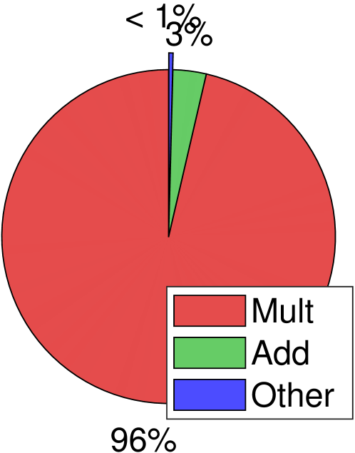
Figure 4: Energy breakdown for different ops.

In the following, we study the energy optimization potential of employing approximate components. As a case study, we select from the EvoApprox8B library [19] the NGR approximate multiplier and the 5LT approximate adder. The results in Fig. 5 show that approximating only the multipliers (XM) can save more than 28% of the energy consumption, compared to the accurate implementation (Acc). Due to the low share of energy consumed by the additions, the advantage of employing approximate adders (XA) or employing approximate adders and multipliers (XAM) is negligible compared to Acc and XM solutions, respectively.

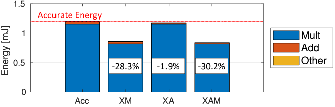
Figure 5: Optimization potential by applying approx. components in CapsNets.

Motivated by the above discussions and analysis, in the following, without loss of generality and for the ease of proof-of-concept development, we focus our analyses on the approximate multipliers, since they have high impact on the energy consumption, thus opening huge optimization potentials.

III-B Error Profiles for the Approximate Hardware Multipliers

We selected 35 approximate multipliers from the EvoApprox8B library [19] and analyzed the distributions of the erroneous products $P^{\prime}$ generated by such multipliers, compared to the accurate product $P$ of an 8-bit multiplier (i.e., 16-bit output). The arithmetic error is computed in Eq. 2, where $a,b$ denotes the inputs to the multipliers from a representative set of inputs $I$.

$$\Delta_{P^{\prime}}=\{\forall a,b\in I:P^{\prime}(a,b)-P(a,b)\}$$ (2)

The distributions of the arithmetic errors are calculated as having a single multiplier, a sequence of 9 multiply-and-accumulate (MAC) units, and as a sequence of 81 MAC units, with $|I|=10^{5}$ random samples per each scenario. These analyses are performed for estimating the accumulated error of a convolution with $3\times 3$ and $9\times 9$ filters, respectively. We selected these values because they reflect the size of the convolutional kernels of the DeepCaps [24] and CapsNet [25].

The majority of the components (31 of 35) has a Gaussian-like distribution of the arithmetic error $\Delta$, with a mean value m and a standard deviation std. The error distributions of two approximated multipliers from [19] are shown in Fig. 6.

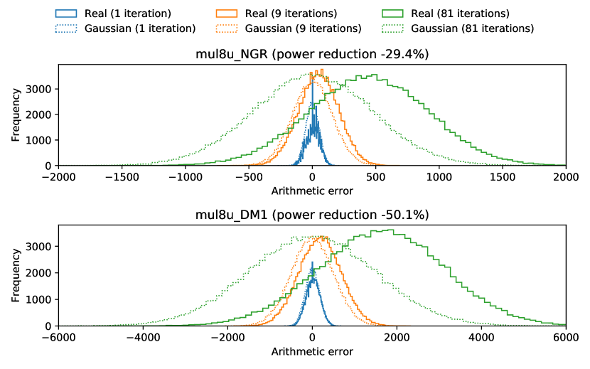
Figure 6: Artimetic error (w.r.t. accurate 8-bit multiplier) distributions and their interpolations by Gaussian noise by having an approximate multiplier from the EvoApprox8B library [19]. (top) Distribution for the NGR multiplier. (bottom) Distribution for the DM1 multiplier.

Modeling a Gaussian noise $\Delta$, when employing $b$-bit fixed-point approximate components in a CapsNet which has floating-point operations, is an open research problem. We propose to adjust the noise w.r.t. the range $R$ of values of a given array $X$. Hence, we introduce the noise magnitude ($NM$) to indicate the standard deviation ($std$) of the noise $\Delta$ scaled w.r.t. $R(X)$, and the noise average ($NA$) to indicate the mean value ($m$) of the noise $\Delta$ scaled w.r.t. $R(X)$.

$$NM(\Delta_{M})=\frac{stdev(\Delta_{X})}{R(X)},\ NA(\Delta_{M})=\frac{m(\Delta_{X})}{R(X)}$$

Since the inputs of components ($I$) employed in CapsNets have typically some specific distribution patterns, the $NM$ of the approximate component is dependent on the application. This implies that the $NM$ can change significantly for different CapsNet models and different dataset used. Hence, we show several experiments for different benchmarks in Sec. VI.

III-C Noise Injection Modeling

Based on the above analysis, without loss of generality, we can model the error source coming from approximate components as a Gaussian random noise added to the array $X$ under consideration.

An error with certain values of $NM$ and $NA$, associated to a given tensor $X$ (i.e., a multidimensional output of a CapsNet operation) with shape $s$ is modelled as in Equation 3. The noisy output is denoted as $X^{\prime}$ in Equation 4.

$$\Delta_{X}=Gauss(s,(NM\cdot R(X)))+(NA\cdot R(X))$$ (3)

$$X^{\prime}=X+\Delta_{X}\vspace*{-0mm}$$ (4)

Here, $Gauss(s,std)+m$ is a function which generates a tensor of random numbers with shape $s$, following a Gaussian distribution with mean $m$ and standard deviation $std$.

IV ReD-CaNe: Our Methodology for Error Resilience Analysis and Design of Approximate CapsNets

Our methodology is composed of 6 steps, as shown in Fig. 7. Once we identify the lists of arrays in which we want to inject noise, called Groups, we apply the noise injection, as described in Sec. III-C. By monitoring the impact on the test accuracy of different arrays of operations, we can identify the most and the least critical operations in a given CapsNet from the accuracy point of view. Therefore, our ReD-CANE methodology can provide useful guidelines for designing energy-efficient inference, showing the potential to apply approximations to specific layers and operations (i.e., the more resilient ones) without significantly sacrificing the accuracy. A step-by-step flow of our methodology is described in the following:

1. Group Extraction: We divide the operations of the CapsNet inference into groups, based on the type of operation (e.g., MAC, activation function, softmax or logits update). This step generates the Groups.

2. Group-Wise Resilience Analysis: We monitor the test accuracy drop by injecting noise to different groups.

3. Mark Resilient Groups: Based on the results of the analysis performed at the Step 2, we mark the more resilient groups. After this step, there are two categories of Groups, the Resilient and Non-Resilient ones.

4. Layer-Wise Resilience Analysis for Non-Resilient Groups: For each non-resilient group, we monitor the test accuracy drop by injecting noise at each layer.

5. Mark Resilient Layers for Each Non-Resilient Group: Based on the results of the analysis performed at the Step 4, we mark the more resilient layers.

6. Select Approximate Components: For each operation, we select approximate components from a given library, based on the resilience measured as the noise magnitude $(NM)$.

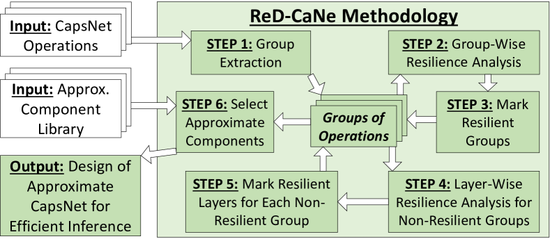
Figure 7: ReDCaNe: our methodology for resilience analysis and design of Approximate CapsNets.

Note, a step of resilience analysis consists of setting the input parameters of the noise injection, i.e., $NM$ and $NA$, to add the noise to the selected CapsNet operations, and monitoring the accuracy for the noisy CapsNet.

The output of our methodology is the approximated version of a given CapsNet, which is ready to be executed in a specialized hardware accelerator for inference with approximate components. For the purpose of saving area and energy, we select, for each operation, the approximate components, from a given library, that correspond to their level of resilience. Hence, more aggressive approximations are selected for more resilient operations, without significantly affecting the classification accuracy of the CapsNet inference.

V Experimental setup

The experimental setup is shown in Fig. 8. We train a given CapsNet model for a given dataset using TensorFlow [1], running on two Nvidia GTX 1080 Ti GPUs. The trained model serves as an input to our ReD-Cane methodology. The noise is injected to the arrays and then the accuracy is monitored to identify the resilience of the operations.

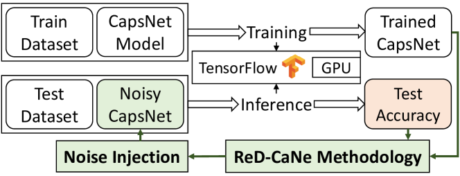
Figure 8: Experimental setup for our simulations.

V-A CapsNet Models and Datasets

We test our methodology on two networks, the DeepCaps [24] and the original CapsNet [25]. We use the datasets CIFAR-10 [13], SVHN [22], MNIST [14], and Fashion-MINST [29], to classify generic images, house numbers, handwritten digits, and fashion clothes, respectively. The accuracy results obtained by training these networks for different datasets are reported in Table II. Table III shows the partition of the CapsNet operation into groups, which is then used for the group extraction step.

TABLE II: Classification accuracy results using accurate multipliers.

Architecture	Dataset	Accuracy
DeepCaps [24]	CIFAR-10	92.74
	SVHN	97.56
	MNIST	99.72
CapsNet [25]	Fashion-MNIST	92.88
	MNIST	99.67

TABLE III: Grouping the operations of the CapsNet inference.

#	Group Name	Description
1	MAC Outputs	Outpus of the matrix multiplications
2	Activations	Output of the activation functions (RELU or SQUASH)
3	Softmax	Results of the softmax (k coefficnents in dynamic routing)
4	Logits Update	Update of the logits (b coefficients in dynamic routing)

V-B TensorFlow Implementation

The proposed methodology is implemented in TensorFlow [1]. First, the network is trained using standard approaches. We modified the computational graph in protobuf format by including our noise injection model in the Graph tool. We implemented a specialized node for the noise injection, where the values of $NA$ and $NM$ can be specified as inputs to this node. Hence, for each node $\tau$, a new set of nodes $T$ is added to the graph. The nodes in $T$ have the same shape as $\tau$ and they consist of the set of operations for adding a Gaussian noise with $std=NM\cdot R(\tau)$ and $m=NA\cdot R(\tau)$, given the range $R$ of the node $\tau$.

V-C Approximate Multiplier Library

We use the EvoApprox8b library, which consists in 35 8-bit unsigned components. We select 8-bit wordlength since it was shown to be enough accurate in the computational path of CapsNets [17].

VI Experimental Results

VI-A Detailed Analysis for the CIFAR-10 Dataset

As a case study analysis, we report detailed results for the DeepCaps on the CIFAR-10 datasets. The results for other benchmarks are reported in Section VI-C.

For the following analyses, we used a $NM\in[0.5\dots 0.001]$. To analyze the general case of error resilience, we selected the average error $NA=0$. In the experiment for the Step 2 of our methodology, we inject the same noise to every operation within a group, while keeping the other groups accurate. From the results shown in Fig. 9, we notice that the Softmax and the Logits update groups are more resilient than MAC outputs and Activations, because the CapsNet accuracy starts to decrease with a correspondent lower $NM$. Note, for low $NM$, the noise injection slightly increases the accuracy due to regularization, with a similar effect as the dropout [27].

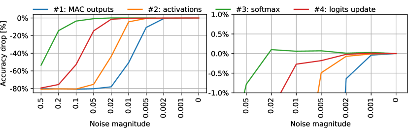
Figure 9: Group-wise resilience for the CIFAR-10 dataset. (left) Complete results. (right) Zoomed view of the accuracy drop, centered at $0\%$.

In Fig. 10, we analyze the resilience of each layer of the non-resilient groups (i.e., MAC outputs and Activations). We notice that the first convolutional layer is the least resilient, followed by the layers in the middle. Moreover, the Caps3D layer is the most resilient one. Since this layer is the only convolutional layer that employs the dynamic routing algorithm, we correlate the higher resilience to the iterations performed in this layer, because the coefficients are updated dynamically at run-time, thus they can adapt to the noise.

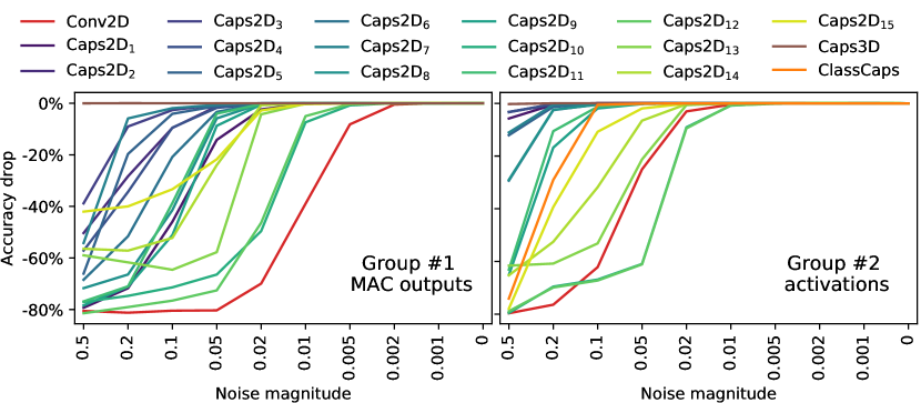
Figure 10: Layer-wise analysis of the non-resilient groups for CIFAR-10 dataset. The noise is injected in (left) the MAC outputs and (right) the activations.

VI-B Evaluating the Selection of Approximate Components

The choice of the approximate component for each operation depends on the level of $NM$ corresponding to a tolerable accuracy loss, which is typically null or very low. Recalling Eq. 2, the parameters $NM$ and $NA$ are dataset dependent because their values change accordingly to the input range $R$. In our case study (DeepCaps for CIFAR-10), we select a subset of $10^{6}$ elements from the inputs of every Conv2D layers of the DeepCaps, with its corresponding distribution (frequency of occurrence) shown in Fig. 11 (left). The distribution is approximately Gaussian, but there is a peak between $40$ and $50$ for the input feature maps, which is caused by a specific distribution of the input dataset. Indeed, the peak occurs in the first Caps2D layer, as shown in Fig. 11 (right).

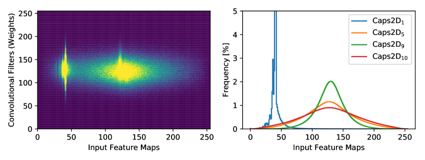
Figure 11: (left) Distribution of $10^{6}$ random samples from the inputs of the convolutions in the DeepCaps for the CIFAR-10 dataset. (right) A focus on some layers, showing the peak in the first Caps2D layer.

Hence, we measure the $NM$ and $NA$ parameters of the selected multipliers in the library (Tab. IV). We use two different input distributions, the modeled one that is based on random inputs generated with a uniform distribution, and the real one, which is based on the input distribution previously shown in Fig. 11. Note, these values slightly differ, because the $NM$ and $NA$ parameters are dataset dependent. The major differences are due to an overestimation of the $NM$ and $NA$ by our modeled distribution. Therefore, the selection of approximate components based on our models can be systematically employed for designing approximate CapsNets.

TABLE IV: Power, area, and noise magnitude, computed with a modeled input dataset (with uniform distribution) and with a real input distribution $I$, for different^∗ approximated multipliers from the EvoApprox8B library [19].

Multiplier	Power	Area	Modeled $\Delta_{X}$		Real $\Delta_{X}$
mul8u_	$\mu$W	$\mu$m2	$NA$	$NM$	$NA$	$NM$
1JFF	391 (-0%)	710 (-0%)	0.0000	0.0000	0.0000	0.0000
14VP	364 (-7%)	654 (-8%)	0.0000	0.0001	0.0000	0.0001
GS2	356 (-9%)	633 (-11%)	0.0004	0.0017	0.0001	0.0013
CK5	345 (-12%)	604 (-15%)	0.0000	0.0002	0.0000	0.0002
7C1	329 (-16%)	607 (-14%)	0.0011	0.0033	0.0007	0.0026
96D	309 (-21%)	605 (-15%)	0.0035	0.0077	0.0020	0.0051
2HH	302 (-23%)	542 (-24%)	-0.0001	0.0007	-0.0001	0.0007
NGR	276 (-29%)	512 (-28%)	0.0001	0.0008	0.0002	0.0009
19DB	206 (-47%)	396 (-44%)	0.0010	0.0019	0.0010	0.0021
DM1	195 (-50%)	402 (-43%)	0.0003	0.0025	0.0005	0.0025
12N4	142 (-64%)	390 (-45%)	0.0018	0.0054	0.0019	0.0056
1AGV	95 (-76%)	228 (-68%)	0.0027	0.0080	0.0026	0.0117
YX7	61 (-84%)	221 (-69%)	0.0484	0.0741	0.0268	0.0347
JV3	34 (-91%)	111 (-84%)	0.0021	0.0267	-0.0028	0.0301
QKX	29 (-93%)	112 (-84%)	0.0509	0.0736	0.0293	0.0350
∗We have randomly selected 14 components, representative for the complete library.

VI-C Testing our Methodology on Different Benchmarks

We apply our methodology to the other benchmarks. The results coming from the resilience analysis of the Step 2 are shown in Fig. 12. A key property that we can observe is that MAC outputs and activations are less resilient than the other two groups. Moreover, we noticed that the logits update on the CapsNet [25] for MNIST (bottom right) is slightly less resilient than the same group on the DeepCaps [24] for MNIST (top right), because the CapsNet has only one layer that performs Dynamic routing, while the DeepCaps has two.

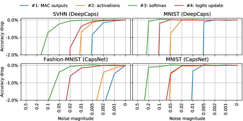
Figure 12: Group-wise resilience for different benchmarks.

VI-D Results Discussion

From our analyses, we can derive that the CapsNets have interesting resilience properties. A key observation, valid for every benchmark, is that the layers computing the the dynamic routing (ClassCaps and Caps3D), and the corresponding groups of operations (softmax and logits update) are more resilient than others. Such outcome is attributed to a common feature of the dynamic routing. The values of the involved coefficients (logits $b$ and coupling coefficients $k$, see Fig. 3) are updated dynamically, thereby adapting to the injected noise. Hence, more aggressive approximations can be tolerated for these computations.

VII Conclusion

We proposed a systematic methodology for analyzing the resilience of CapsNets under approximation errors that can provide foundation to design approximate CapsNet hardware. We designed an error injection model, which accounts for the approximation errors. We modeled the errors of applying approximate multipliers in the computational units of CapsNet accelerators. We systematically analyzed the (group-wise and layer-wise) resilience of the operations and designed approximated CapsNets, based on different resilience levels. We showed that the operations in the dynamic routing are more resilient to approximation errors. Hence, more aggressive approximations can be adopted for these computations, without sacrificing the classification accuracy much. Our methodology provides the first step towards real-world approximate CapsNets to realize their energy-efficient inference.

References

- Abadi et al. [2016] M. Abadi et al. Tensorflow: A system for large-scale machine learning. In USENIX, 2016.
- Du et al. [2014] Z. Du et al. Leveraging the error resilience of machine-learning applications for designing highly energy efficient accelerators. In ASP-DAC, 2014.
- Goodfellow et al. [2015] I. Goodfellow et al. Explaining and harnessing adversarial examples. ICLR, 2015.
- Han et al. [2016a] S. Han, X. Liu, et al. EIE: efficient inference engine on compressed deep neural network. In ISCA, 2016a.
- Han et al. [2016b] S. Han et al. Deep compression: Compressing deep neural network with pruning, trained quantization and huffman coding. In ICLR, 2016b.
- Hanif et al. [2019] M. A. Hanif, F. Khalid, and M. Shafique. CANN: curable approximations for high-performance deep neural network accelerators. In DAC, 2019.
- Hanif et al. [2018] M. A. Hanif et al. Error resilience analysis for systematically employing approximate computing in convolutional neural networks. In DATE, 2018.
- Hanif et al. [2018] M. A. Hanif et al. X-dnns: Systematic cross-layer approximations for energy-efficient deep neural networks. J. Low Power Electronics, 2018.
- Hinton et al. [2011] G. E. Hinton et al. Transforming auto-encoders. In ICANN, 2011.
- Jacob et al. [2017] B. Jacob et al. Quantization and training of neural networks for efficient integer-arithmetic-only inference, 2017.
- Jiao et al. [2017] X. Jiao et al. An assessment of vulnerability of hardware neural networks to dynamic voltage and temperature variations. In ICCAD, 2017.
- Kim et al. [2014] Y. Kim et al. Flipping bits in memory without accessing them: An experimental study of dram disturbance errors. In ISCA, 2014.
- Krizhevsky [2009] A. Krizhevsky. Learning multiple layers of features from tiny images. 2009.
- Lecun et al. [1998] Y. Lecun et al. Gradient-based learning applied to document recognition. 1998.
- Li et al. [2017] G. Li et al. Understanding error propagation in deep learning neural network (dnn) accelerators and applications. In SC, 2017.
- Liu et al. [2017] Y. Liu et al. Fault injection attack on deep neural network. In ICCAD, 2017.
- Marchisio et al. [2019] A. Marchisio, M. A. Hanif, and M. Shafique. Capsacc: An efficient hardware accelerator for capsulenets with data reuse. In DATE, 2019.
- Marchisio et al. [2019] A. Marchisio et al. Deep learning for edge computing: Current trends, cross-layer optimizations, and open research challenges. In ISVLSI, 2019.
- Mrazek et al. [2017] V. Mrazek et al. Evoapproxsb: Library of approximate adders and multipliers for circuit design and benchmarking of approximation methods. DATE, 2017.
- Mrazek et al. [2019a] V. Mrazek et al. ALWANN: automatic layer-wise approximation of deep neural network accelerators without retraining. In ICCAD, 2019a.
- Mrazek et al. [2019b] V. Mrazek et al. autoax:an automatic design space exploration and circuit building methodology utilizing libraries of approximate components. DAC, 2019b.
- Netzer et al. [2011] Y. Netzer et al. Reading digits in natural images with unsupervised feature learning. In NIPS W., 2011.
- Parashar et al. [2010] K. Parashar et al. A hierarchical methodology for word-length optimization of signal processing systems. In VLSID, 2010.
- Rajasegaran et al. [2019] J. Rajasegaran et al. Deepcaps: Going deeper with capsule networks. CVPR, 2019.
- Sabour et al. [2017] S. Sabour et al. Dynamic routing between capsules. In NIPS. 2017.
- Srinivasan et al. [2016] G. Srinivasan et al. Significance driven hybrid 8t-6t sram for energy-efficient synaptic storage in artificial neural networks. In DATE, 2016.
- Srivastava et al. [2014] N. Srivastava et al. Dropout: A simple way to prevent neural networks from overfitting. JMLR, 2014.
- Wu et al. [2019] X. Wu et al. Speech emotion recognition using capsule networks. ICASSP, 2019.
- Xiao et al. [2017] H. Xiao et al. Fashion-mnist: a novel image dataset for benchmarking machine learning algorithms. 2017.
- Yu et al. [2019] Y. Yu et al. Vehicle detection from high-resolution remote sensing imagery using convolutional capsule networks. GRSL, 2019.
- Zhang et al. [2019] J. J. Zhang, K. Basu, and S. Garg. Fault-tolerant systolic array based accelerators for deep neural network execution. IEEE Design Test, 2019.
- Zhang et al. [2019] J. J. Zhang et al. Building robust machine learning systems: Current progress, research challenges, and opportunities. In DAC, 2019.
- Zhao et al. [2019] W. Zhao, H. Peng, S. Eger, E. Cambria, and M. Yang. Towards scalable and reliable capsule networks for challenging nlp applications, 2019.