Stochastic Variational Inference via Upper Bound

Abstract

Stochastic variational inference (SVI) plays a key role in Bayesian deep learning. Recently various divergences have been proposed to design the surrogate loss for variational inference. We present a simple upper bound of the evidence as the surrogate loss. This evidence upper bound (EUBO) equals to the log marginal likelihood plus the KL-divergence between the posterior and the proposal. We show that the proposed EUBO is tighter than previous upper bounds introduced by $\chi$-divergence or $\alpha$-divergence. To facilitate scalable inference, we present the numerical approximation of the gradient of the EUBO and apply the SGD algorithm to optimize the variational parameters iteratively. Simulation study with Bayesian logistic regression shows that the upper and lower bounds well sandwich the evidence and the proposed upper bound is favorably tight. For Bayesian neural network, the proposed EUBO-VI algorithm outperforms state-of-the-art results for various examples.

1 Introduction

Stochastic variational inference (SVI) plays a key role in Bayesian deep learning. SVI solves the Bayesian inference problem by introducing a variational distribution $q(\theta;\lambda)$ over the latent variables $\theta$ [11, 7], and then minimizes the Kullback-Leibler (KL) divergence between the approximating distribution $q(\theta;\lambda)$ and the exact posterior $p(\theta|\mathcal{D})$. This minimization is the same as maximizing the evidence lower bound (ELBO), $\mathcal{L}=\int q(\theta;\lambda)[\log p(\mathcal{D},\theta)-\log q(\theta;\lambda)$ [11], which is a lower bound of the model evidence $\log p(\mathcal{D})$. The KL-divergence is the discrepancy between the surrogate loss ELBO and the evidence. SVI turns the Bayesian inference into an optimization problem. It has been recognized that the property of discrepancy has strong influence on the optimization of ELBO [15, 2, 22]. The classical objective $D_{\mathrm{KL}}(q(\theta;\lambda)||p(\theta|\mathcal{D}))$ leads to approximate the posteriors with zero-forcing behavior. This zero-forcing behavior imposes undesirable properties, which may lead to underestimation of the posterior’s support especially when dealing with light-tailed posteriors or multi-modal posteriors [17, 5, 2]. Various SVI methods are proposed to use different divergences to achieve tighter bound and/or mass-covering property, which may lead to better performance in SVI [15, 2, 21]. Recently, the upper bound of $\log p(D)$ has captured certain attention. For instance, the variational Rényi bound ($\mathcal{L}_{\alpha}(\lambda)=\frac{1}{1-\alpha}\log E_{q}[(\frac{p(\mathcal{D},\theta)}{q(\theta;\lambda)})^{1-\alpha}]$, for $\alpha\neq 1$) and the $\chi$ upper bound ($\mathcal{L}_{\chi^{n}}(\lambda)=\frac{1}{n}\log E_{q}[(\frac{p(\mathcal{D},\theta)}{q(\theta;\lambda)})^{n}]$, for $n>1$) are introduced to provide the mass-covering property: optimizing such divergence leads to a variational distribution with a mass-covering (or say zero-avoiding) behavior. The resulting gradient of $\alpha$-divergence based upper bound is,

$$\mathcal{\nabla_{\lambda}L}_{\alpha}=\frac{1}{1-\alpha}\mathbb{E}_{q}\left[w_{\alpha}\nabla_{\lambda}(\log p(\mathcal{D},\theta)-\log q(\theta;\lambda))\right]$$ (1)

where $\nicefrac{{w_{\alpha}=\left(\frac{p(\mathcal{D},\theta)}{q(\theta;\lambda)}\right)^{1-\alpha}}}{{E_{q}\left[\left(\frac{p(\mathcal{D},\theta)}{q(\theta;\lambda)}\right)^{1-\alpha}\right]}}$ [15]. Interestingly, we have the connection that when $\alpha\rightarrow 1$, the Rényi- divergence become the KL-divergence and the Rényi-VI algorithm reduces to the standard SVI [7]; when $\alpha=0$ , the Rényi-VI becomes the importance weighted auto-encoder (IWAE) or say the importance weighted VI[1, 3]; when $\alpha=-1$ , it becomes the $\chi^{2}$ divergence based CHIVI algorithm [2]. The integration in the gradient $\mathcal{\nabla_{\lambda}L}_{\alpha}$ can be estimated by Monte Carlo approach with samples drawn from $q(\theta;\lambda)$. Then the stochastic gradient descendant (SGD) algorithm is applied to optimize the variational parameter $\lambda$. Moreover, to deal with large datasets, we may use a minibatch of the data $\mathcal{D}$ in the evaluation of the joint distribution $p(\mathcal{D},\theta)$ [19]. Inspired by these previous works, here we explore a simple but effective upper bound for variational inference, our main contributions are summarized:

1. We propose a new upper bound of the evidence by introducing the KL-divergence between the posterior and the variational distribution. The proposed EUBO possess the mass covering properties, and is tighter then the upper bounds introduced by $\alpha$-divergence or $\chi$-divergence.

2. We present the numerical approximation of the gradient of the EUBO, apply the SGD algorithm to optimize the variational parameters, and format a black-box style variational inference which is suitable for scalable Bayesian inference.

3. With the upper and lower bound sandwiching the evidence, we can be more confident to evaluate the fitting of model. We also find that the EUBO converges faster and is tighter than the ELBO. In Bayesian neural network regression, the EUBO-VI algorithm gains improvement in both the test error and the model fitting.

2 Variational Inference with the EUBO

2.1 Upper bound of the model evidence

As it is well known that the KL-divergence is not symmetric, $D_{\mathrm{KL}}(q||p)$ possesses the zero-force property, but the inverse KL-divergence $D_{\mathrm{KL}}(p||q)$ posses the mass-covering property. This motivates our work to leverage on $D_{\mathrm{KL}}(p||q)$ in the design of the surrogate loss. By using Gibbs’ inequality that $-\int p(\theta|\mathcal{D})\log p(\theta|\mathcal{D})d\theta\leq-\int p(\theta|\mathcal{D})\log q_{\lambda}(\theta)d\theta$ holds for any distribution $q(\theta;\lambda)$, we introduce an upper bound on the model evidence,

$$\log p(\mathcal{D}) =\int p(\theta|\mathcal{D})\log p(\mathcal{D},\theta)d\theta-\int p(\theta|\mathcal{D})\log p(\theta|\mathcal{D})d\theta$$

$$\leq\int p(\theta|\mathcal{D})\log p(\mathcal{D},\theta)d\theta-\int p(\theta|\mathcal{D})\log q(\theta;\lambda)d\theta=\int p(\theta|\mathcal{D})\log\frac{p(\mathcal{D},\theta)}{q(\theta;\lambda)}$$ (2)

We define $\mathcal{U}(\lambda)\equiv\int p(\theta|\mathcal{D})\log\dfrac{p(\mathcal{D},\theta)}{q(\theta;\lambda)}d\theta$ as the Evidence Upper BOund (EUBO). It is easy to find that $\mathcal{U}(\lambda)=\log p(\mathcal{D})+\mathrm{D_{KL}}(p(\theta|\mathcal{D})||q(\theta;\lambda))$, that is $D_{\mathrm{{KL}}}(p(\theta|\mathcal{D})||q(\theta;\lambda))$ just the discrepancy between the EUBO $\mathcal{U}(\lambda)$ and the true $\log p(\mathcal{D})$.

2.2 Some properties of the EUBO

We present three favorable properties of the proposed EUBO $\mathcal{U}(\lambda)$. First the discrepancy $D_{\mathrm{{KL}}}(p(\theta|\mathcal{D})||q(\theta;\lambda))$ possesses mass covering property. According to previous studies[15, 2], the mass covering property has advance in approximation of the posterior. The mass covering property of EUBO, can be easily verified by simulation examples [16, 8]. Second, $D_{\mathrm{{KL}}}(p(\theta|\mathcal{D})||q(\theta;\lambda))$ is a tight discrepancy. We find that the $D_{\mathrm{{KL}}}(p(\theta|\mathcal{D})||q(\theta;\lambda))$ proposed in this work is tighter than the $\alpha$-divergence and $\chi^{n}$-divergence. With this tighter discrepancy, we can then design tighter upper bounds. As discussed in [1, 21], tighter bound tends to lead better performance in SVI. We present a theorem to show the advantage of the proposed EUBO (see the appendix for a brief proof).

Theorem 1. Define the EUBO as equation (2). Then the following holds:

• ELBO $\mathcal{L}(\lambda)$ $\leq\log p(\mathcal{D})\leq$ EUBO $\mathcal{U}(\lambda)$.

• $D_{\alpha}(q(\theta)||p(\theta|\mathcal{D}))\geq\frac{-\alpha}{1-\alpha}D_{\mathrm{{KL}}}(p(\theta|\mathcal{D})||q(\theta))$ , for $\alpha\leq 0$; $D_{\chi^{n}}(q(\theta)||p(\theta|\mathcal{D}))\geq\frac{n-1}{n}D_{\mathrm{{KL}}}(p(\theta|\mathcal{D})||q(\theta))$, for $n\geq 2$.

• $\frac{-\alpha}{1-\alpha}\mathcal{U}(\lambda)+\frac{1}{1-\alpha}\log p(\mathcal{D})\leq\mathcal{U}_{\alpha}(\lambda)$, for $\alpha\leq 0$ ; $\frac{n-1}{n}\mathcal{U}(\lambda)+\frac{1}{n}\log p(\mathcal{D})\leq\mathcal{U}_{\chi^{n}}(\lambda)$, for $n\geq 2$.

Third, the numerical estimation of EUBO is close to the ground true evidence, even when the variational distribution has not been well optimized. The EUBO involves an integration with respect to the unknown posterior. As stated in later section, we use importance sampling in the estimation of this upper bound. The using of importance sampling reduces the bias of the MC estimation of the evidence when the variational proposal has certain discrepancy with the posterior. This property leads to two advantage: 1) model selection based solely on the ELBO is inappropriate because of the possible variation in the tightness of this bound, with the accompanying upper bound to sandwich the evidence, one can perform model selection with more confidence[4, 10]; 2) in case we need to evaluate the evidence or its surrogate when the optimization process of variational parameters can run only few steps, for example in the Bayesian Meta-learning[12, 20], the proposed EUBO may be preferable since its estimation is insensitive to the bias of variational distribution.

2.3 SGD for the EUBO

By definition, the EUBO $\mathcal{U}(\lambda)$ has an integration with respect to unknown posterior. In previous study[9, 10], the posterior is represented by simulated sample from Markov chain Monte Carlo (MCMC), and the integration is approximated via Monte Carlo. However, Monte Carlo particularly MCMC is not a scalable method in dealing with large scale Bayesian learning problem. Following the idea of black-box VI[19], we use only a few number of Monte Carlo samples to obtain a ‘noisy’ gradient of the EUBO, and then apply the SGD approach to optimize $\lambda$ iteratively. First, we derive the gradient of $\mathcal{U}(\lambda)$ (refer to the Appendix for details), denoted by $\nabla_{\lambda}\mathcal{U}$,

$$\nabla_{\lambda}\mathcal{U}=\mathbb{E}_{q}\left\{w(\theta)\left[(\log\omega(\theta)+1)\nabla_{\lambda}\log p(\mathcal{D},\theta)-\nabla_{\lambda}\log q(\theta;\lambda)\right]\right\}$$ (3)

where $w(\theta)=\frac{p(\theta|D)}{q(\theta;\lambda)}$ and $\omega(\theta)=\frac{p(D,\theta)}{q(\theta;\lambda)}.$ Note that the posterior $p(\theta|\mathcal{D})$ in $w(\theta)$ is generally unknown, so we use the joint distribution $p(\mathcal{D}|\theta)p(\theta)$ instead and normalizes the weights to cancel the unknown constant $p(\mathcal{D})$. Given the samples $\{\theta^{(i)}\}_{i=1}^{M}$ drawn from $q(\theta;\lambda)$ and normalized weights $\{\hat{w}^{(i)}\}_{i=1}^{M}$, we estimate $\nabla_{\lambda}\mathcal{U}$ as follows,

$$\hat{\nabla}_{\lambda}\mathcal{U}=\sum_{i}^{M}\hat{w}^{(i)}\left[(\log\omega(\theta^{(i)})+1)\nabla_{\lambda}\log p(\mathcal{D},\theta^{(i)})-\nabla_{\lambda}\log q(\theta^{(i)};\lambda)\right].$$ (4)

To deal with large dataset, we divide the entire dataset to mini-batch. Only a mini-batch data $\mathcal{S}=\{x_{n}\}_{n=1}^{S}$ is used in the evaluation of $p(\mathcal{D},\theta)$,

$$p(\mathcal{D},\theta^{(i)})\approx\left[\prod_{n=1}^{S}p(x_{n}|\theta^{(i)})\right]^{\frac{N}{S}}p(\theta^{(i)}).$$

To incorporate with the advantage of autogradient packages , we take the reparametrization trick [13] that $\theta^{(i)}=g_{\lambda}(\epsilon^{(i)})=\mu+\sigma\text{$\epsilon^{(i)}$}$, where $\lambda=[\mu,\sigma]$ and $\epsilon^{(i)}\sim\mathcal{N}(0,1)$, then the resulting reparameterization gradient becomes,

$$\hat{\nabla}_{\lambda}\mathcal{U}=\sum_{i}^{M}\hat{w}^{(i)}\left[(\log\omega(\theta^{(i)})+1)\nabla_{\lambda}\log p(\mathcal{D},g_{\lambda}(\epsilon^{(i)}))-\nabla_{\lambda}\log q(g_{\lambda}(\epsilon^{(i)});\lambda)\right].$$ (5)

This reparametrization trick significantly reduces the effort needed to implement variational inference in a wide variety of models. Finally, with the noisy estimation of the gradient $\hat{\nabla}_{\lambda}\mathcal{U}$, the SGD algorithm is applied to minimize the EUBO iteratively, $\lambda_{t+1}=\lambda_{t}-\alpha*\hat{\nabla}_{\lambda}\mathcal{U}$. The algorithm is presented as follows,

Algorithm 1 EUBO based variational inference (EUBO-VI)

• Initialization: initialize the parameter $\lambda_{0}$ randomly or by some pre-specified values, the learning rate $\alpha_{0}$.

• for $t=0,...,T$

  • pick up a mini-batch data $\mathcal{S}=\{x_{n}\}_{n=1}^{S}$.

  • generate $M$ samples $\{\theta^{(i)}\}_{i=1}^{M}$ : $\epsilon^{(i)}\sim\mathcal{N}(0,1)$ , $\theta^{(i)}=g_{\lambda}(\epsilon^{(i)}=\mu+\sigma\text{$\epsilon^{(i)}$}$.

  • calculate the weight $\log w^{(i)}=\frac{N}{S}\sum_{n=1}^{S}\log p(x_{n}|\theta^{(i)})+\log p(\theta^{(i)})-\log q(\theta^{(i)};\lambda_{t})$, $w^{(i)}=\exp\left(\log w^{(i)}-\max\{\log w^{(i)}\}\right)$, and normalize $\hat{w}^{(i)}=\frac{w^{(i)}}{\sum_{i}w^{(i)}}$ .

  • evaluate the gradient $\hat{\nabla}_{\lambda}\mathcal{U}=-\sum\hat{w}^{(i)}\nabla_{\lambda}\log q(g_{\lambda}(\epsilon^{(i)})$ .

  • update $\lambda_{t+1}=\lambda_{t}-\alpha_{t}*\hat{\nabla}_{\lambda}\mathcal{U}$ .

After we obtain the optimal $\lambda^{*}$, the resulting minimum upper bound $\mathcal{U}(\lambda)$ is then estimated by

$$\mathcal{\hat{U}^{*}}=\sum_{i=1}^{M}\hat{w}^{(i)}\left[\sum_{n=1}^{N}\log p(x_{n}|\theta^{(i)})+\log p(\theta^{(i)})-\log q(\theta^{(i)};\lambda^{*})\right]$$ (6)

Furthermore, if we assume the posterior $p(\theta|\mathcal{D})$ and the joint distribution $p(\theta,\mathcal{D})$ has no relation to the variational parameter $\lambda$ , which means $\nabla_{\lambda}p(\theta|\mathcal{D})=0$ and $\nabla_{\lambda}\log p(\mathcal{D},\theta)=0$, then we obtain the score gradient, $\hat{\nabla}_{\lambda}\mathcal{U}=-\sum_{i}^{M}\hat{w}^{(i)}\nabla_{\lambda}\log q(\theta^{(i)};\lambda)$. Compare with the score gradient of CHIVI[2], we find the only difference is the definition of $\hat{w}$: $\hat{w}\propto\frac{p(D,\theta)}{q(\theta;\lambda)}$ for our EUBO-VI, while $\hat{w}\propto(\frac{p(D,\theta)}{q(\theta;\lambda)})^{2}$ for CHIVI. However, although there is some similarity between the EUBO-VI and CHIVI/Rényi-VI, EUBO-VI is unique and does not fall into any special case of these previous upper bound based SVI algorithms.

3 Simulation studies

3.1 Bayesian Logistic Regression

For Bayesian logistic regression, we use data sets from the UCI repository: Iris, Pima, Spectf, Wdbc and Ionos. The variate dimension in these data sets range from 5 to 45, including a dimension of all ones to account for offset. We set the prior distribution of the coefficients as $\mathcal{N}(0,1)$, choose the number of importance sampling samples as 10 and the mini-batch size as 100. In our experiments we use the Adam algorithm [14], an adaptive version of SGD which automatically tune the learning rates according to the history of gradients and their variances. We perform experiments with the proposed EUBO-SVI, in comparision with vanilla SVI [18], CHIVI[2] and Rényi-VI [15]. We also compared the optimized bounds obtained by various algorithms: $\mathcal{\hat{L}}$ denotes ELBO from vanilla SVI, $\mathcal{\hat{U}}$ denotes EUBO from the proposed algorithm, $\mathcal{U}_{\chi^{2}}$ denotes the upper bound from CHIVI, $\mathcal{\hat{U}}_{\alpha=-2}$ and $\mathcal{\hat{L}}_{\alpha=2}$ denotes the upper and lower bounds from the Rényi-VI with different $\alpha$-divergences.

Take the logistic regression of Iris dataset as example, we show the estimated bound of ELBO and EUBO of each epoch in Figure 1. We observed that the EUBO converges faster, and is tighter than the ELBO even in the early stage when the variational parameters are not well optimized. We run 20 trails for each bounds, the results are shown in table 1. The upper and lower bounds well bracket the log evidence. With both the lower and upper bounds being close to each other, we are more confidence that the VIs find the true evidence. Moreover, simulation results confirm that $\frac{1}{2}\mathcal{U}(\lambda)+\frac{1}{2}\log p(\mathcal{D})\leq\mathcal{U}_{\chi^{2}}(\lambda)$, which is consistent with Theorem 1 discussed in Section 2.2. To test the performance of prediction, all the datasets are randomly partitioned into 90% for training and 10% for testing, and the results are averaged over 20 random trials. The averaged test error is shown in table 2, which shows that the EUBO-SVI algorithm performs well in model prediction.

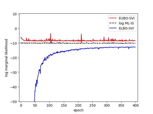
Figure 1: Bayesian logistic regression on Iris data: the upper and lower bounds sandwich the log marginal likelihood.

Table 1: Bayesian logistic regression: estimated upper and lower bounds

	Iris	Pima	Spectf	Wdbc	Ionos
$\mathcal{\hat{U}}_{\alpha=-2}$	-7.94$\pm$0.70	-41$\pm$1.96	-6.20$\pm$1.79	-6.97$\pm$2.24	-28.11$\pm$2.29
$\mathcal{\hat{U}}$	-8.34$\pm$0.37	-44.7$\pm$2.79	-7.53$\pm$1.60	-8.38$\pm$2.39	-30.01$\pm$2.46
$\mathcal{U}_{\chi^{2}}$	-8.58$\pm$0.71	-45.3$\pm$2.07	-8.33$\pm$1.05	$-9.53\pm$1.95	-34.67$\pm$2.11
$\frac{1}{2}\mathcal{\hat{U}}+\frac{1}{2}\log\hat{p}(\mathcal{D})$	-9.18$\pm$0.23	-46.84$\pm$2.21	-9.02$\pm$1.12	-10.84$\pm$2.02	-33.86$\pm$2.18
$\log\hat{p}(\mathcal{D})$	-10.03$\pm$0.17	-48.94$\pm$1.65	-10.51$\pm$0.65	-13.3$\pm$1.65	-37.72$\pm$1.91
$\mathcal{\hat{L}}$	-12.85$\pm$0.27	-53.36$\pm$0.95	-12.58$\pm$0.30	-18.99$\pm$0.29	-46.67$\pm$0.40
$\mathcal{\hat{L}}_{\alpha=2}$	-14.29$\pm$0.55	-55.55$\pm$1.29	-13.19$\pm$0.21	-25.18$\pm$1.04	-51.01$\pm$0.45

Table 2: Bayesian logistic regression: test error

	Iris	Pima	Spectf	Wdbc	Ionos
$D_{\alpha=-2}$-SVI	0.0$\pm$0.0	0.240$\pm$0.043	0.085$\pm$0.046	0.019$\pm$0.013	0.128$\pm$0.070
CHIVI	0.0$\pm$0.0	0.230$\pm$0.038	0.080$\pm$0.062	0.013$\pm$0.013	0.090$\pm$0.039
EUBO-SVI	0.0$\pm$0.0	0.231$\pm$0.045	0.080$\pm$0.055	0.014$\pm$0.012	0.085$\pm$0.045
ELBO-SVI	0.0$\pm$0.0	0.235$\pm$0.040	0.083$\pm$0.058	0.017$\pm$0.012	0.089$\pm$0.046
$D_{\alpha=2}$-SVI	0.0$\pm$0.0	0.229$\pm$0.042	0.081$\pm$0.057	0.014$\pm$0.014	0.088$\pm$0.0394

3.2 Bayesian Neural Network

In the Bayesian neural network regression, we take the same setting with previous work [15]. We use neural networks with one hidden layers, and take 50 hidden units for most datasets, except that we take 100 units for Protein which are relatively large; We set $\mathcal{N}(0,1)$ as the prior distribution for the weight and bias of the neural network. We choose $RELU(x)=max(0,x)$ as the active function. The number of importance sampling samples is 10 and the mini-batch size is 100. All the datasets are randomly partitioned into 90% for training and 10% for testing, and the results are averaged over 20 random trials. We compare our EUBO-VI with state-of-the-art results directly cited from some representative algorithms: Probabilistic backpropagation(BPB)[6], Rényi-VI [15], and CLBO-VI [21]. The averaged prediction accuracy and averaged test log likelihood (LL) are given in Table 3 and Table 4 respectively. The proposed EUBO-VI achieves substantial improvement on both the test error and negative log likelihood for various examples.

Table 3: Bayesian neural network regression: average test RMSE

	EUBO-VI	Rényi-VI[21]	CLBO-VI [21]	ELBO-VI[15]	BPB[6]
Boston	2.62$\pm$0.16	2.86$\pm$0.40	2.71$\pm$0.29	2.89$\pm$0.17	2.977$\pm$0.093
Concrete	4.81$\pm$0.22	5.15$\pm$0.25	5.04$\pm$0.27	5.42$\pm$0.11	5.506$\pm$0.103
Energy	0.94$\pm$0.08	1.00$\pm$0.18	0.95$\pm$0.15	0.51$\pm$0.01	1.734$\pm$0.051
Kin8nm	0.08$\pm$0.00	0.08$\pm$0.00	0.08$\pm$0.00	0.08$\pm$0.00	0.098$\pm$0.001
Naval	0.01$\pm$0.01	0.00$\pm$0.01	0.00$\pm$0.00	0.00$\pm$0.00	0.006$\pm$0.000
Combined	4.07$\pm$0.10	4.13$\pm$0.04	4.03$\pm$0.06	4.07$\pm$0.04	4.052$\pm$0.031
Protein	4.41$\pm$0.05	4.65$\pm$0.07	4.43$\pm$0.05	4.45$\pm$0.02	4.623$\pm$0.009
Wine	0.60$\pm$0.03	0.62$\pm$0.03	0.61$\pm$0.03	0.63$\pm$0.01	0.614$\pm$0.008
Yacht	0.75$\pm$0.05	0.94$\pm$0.23	0.87$\pm$0.18	0.81$\pm$0.05	0.778$\pm$0.042

Table 4: Bayesian neural network regression: average negative test LL(lower is better)

	EUBO-SVI	Rényi-VI[21]	CLBO-VI[21]	ELBO-VI[15]	BPB[6]
Boston	2.37$\pm$0.02	2.46$\pm$0.16	2.40$\pm$0.09	2.52$\pm$0.03	2.579$\pm$0.052
Concrete	2.83$\pm$0.03	3.04$\pm$0.07	3.02$\pm$0.03	3.11$\pm$0.02	3.137$\pm$0.021
Energy	1.63$\pm$0.03	1.67$\pm$0.05	1.65$\pm$0.04	0.77$\pm$0.02	1.981$\pm$0.023
Kin8nm	-1.16$\pm$0.01	-1.14$\pm$0.02	-1.14$\pm$0.02	-1.12$\pm$0.01	-0.901$\pm$0.010
Naval	-3.81$\pm$0.05	-4.11$\pm$0.11	-4.17$\pm$0.01	-6.49$\pm$0.04	-3.735$\pm$0.004
Combined	2.82$\pm$0.01	2.84$\pm$0.04	2.81$\pm$0.02	2.82$\pm$0.01	2.819$\pm$0.008
Protein	2.87$\pm$0.02	2.93$\pm$0.00	2.89$\pm$0.01	2.91$\pm$0.00	2.950$\pm$0.002
Wine	0.92$\pm$0.03	0.94$\pm$0.04	0.93$\pm$0.04	0.96$\pm$0.01	0.931$\pm$0.014
Yacht	1.12$\pm$0.02	1.61$\pm$0.00	1.52$\pm$0.00	1.77$\pm$0.01	1.211$\pm$0.044

4 Conclusion

We investigate the variational inference utilize an effective evidence upper bound (EUBO). The proposed upper bound is based on the KL-divergence between the posterior and variational distribution. We real that this upper bound is tighter than the previous Rényi bound and $\chi$-bound. We proposed the SGD algorithm to optimize the EUBO and develop the reparametrization trick for easy implementation using prevalent python packages for large scale problems. We compare the proposed algorithm with vanilla SVI, CHIVI and Rényi-VI. Simulation study shows that the proposed EUBO-VI algorithm gains improvement on both the test error and log likelihood. We also observed that the EUBO converges faster, and is tighter than the ELBO even in the early stage of the optimization procedure. Moreover, with the both upper and lower bound, we are much confidence with the model fitness. This upper bound VI not only provided for variational inference for complex model, but also provide an easy accessible upper bound for model criticism.

Appendix

Gradient of the EUBO

We present two ways to derive the gradient of the EUBO $\mathcal{U}_{\lambda}$. Reform $\mathcal{U}_{\lambda}$ as an integration with $q(\theta;\lambda)$, that is $\int q(\theta;\lambda)\left(\frac{p(\theta|\mathcal{D})}{q(\theta;\lambda)}\right)\log\frac{p(\mathcal{D},\theta)}{q(\theta;\lambda)}d\theta$, and denote $w(\theta)=\frac{p(\mathcal{D},\theta)}{q(\theta;\lambda)}$ , $\hat{w}(\theta)=\frac{p(\theta|\mathcal{D})}{q(\theta;\lambda)}$ . Note that $\nabla_{\lambda}\log w(\theta)=\nabla_{\lambda}\log\hat{w}(\theta)+\nabla_{\lambda}\log p(D)=\nabla_{\lambda}\log\hat{w}(\theta)$. We can derive the gradient as follows,

$$\nabla_{\lambda}\mathcal{U} = \nabla_{\lambda}\int q(\theta;\lambda)\hat{w}(\theta)\log w(\theta)d\theta$$

$$= \int\nabla_{\lambda}\left[q(\theta;\lambda)\hat{w}(\theta)\log w(\theta)\right]d\theta$$

$$= \int\nabla_{\lambda}q(\theta;\lambda)\hat{w}(\theta)\log w(\theta)d\theta+\int q(\theta;\lambda)\nabla_{\lambda}\hat{w}(\theta)\log w(\theta)d\theta+\int q(\theta;\lambda)\hat{w}(\theta)\nabla_{\lambda}\log w(\theta)d\theta$$

$$= \mathbb{E}_{q}\left[\hat{w}(\theta)\log w(\theta)\nabla_{\lambda}\text{$\log$}q(\theta;\lambda)\right]+\mathbb{E}_{q}\left[\log w(\theta)\nabla_{\lambda}\hat{w}(\theta)\right]+\mathbb{E}_{q}\left[\hat{w}(\theta)\nabla_{\lambda}\log w(\theta)\right]$$

$$= \mathbb{E}_{q}[\hat{w}(\theta)\log w(\theta)\nabla_{\lambda}\text{$\log$}q(\theta;\lambda)]+\mathbb{E}_{q}[\log w(\theta)\hat{w}(\theta)\nabla_{\lambda}\log w(\theta)]+\mathbb{E}_{q}[\hat{w}(\theta)\nabla_{\lambda}\log w(\theta)]$$

$$= \mathbb{E}_{q}[\hat{w}(\theta)\log w(\theta)\nabla_{\lambda}\text{$\log$}q(\theta;\lambda)]+\mathbb{E}_{q}[\log w(\theta)\hat{w}(\theta)\text{($\nabla_{\lambda}$}\log p(\mathcal{D},\theta)-\nabla_{\lambda}\log q(\theta;\lambda))]+\mathbb{E}_{q}[\hat{w}(\theta)\nabla_{\lambda}\log w(\theta)]$$

$$= \mathbb{E}_{q}[\hat{w}(\theta)\log w(\theta)\nabla_{\lambda}\log p(\mathcal{D},\theta)\text{]}+\mathbb{E}_{q}[\hat{w}(\theta)\text{[$\nabla_{\lambda}$}\log p(\mathcal{D},\theta)-\nabla_{\lambda}\log q(\theta;\lambda)]d\theta$$

$$= \mathbb{E}_{q}[\hat{w}(\theta)(\log w(\theta)+1)\nabla_{\lambda}\log p(\mathcal{D},\theta)]-\mathbb{E}_{q}[\hat{w}(\theta)\nabla_{\lambda}\log q(\theta;\lambda)]$$

In another way, we assume the posterior $p(\theta|\mathcal{D})$ and the joint distribution $p(\mathcal{D},\theta)$ has no relation to the parameter $\lambda$ of the variational distribution, that is $\nabla_{\lambda}p(\theta|\mathcal{D})=0$ and $\nabla_{\lambda}\log p(\mathcal{D},\theta)=0$. So we have,

$$\nabla_{\lambda}\mathcal{U} = \nabla_{\lambda}\int p(\theta|\mathcal{D})\log\frac{p(\mathcal{D},\theta)}{q(\theta;\lambda)}d\theta$$

$$= \int\nabla_{\lambda}\left[p(\theta|\mathcal{D})(\log p(\mathcal{D},\theta)-\log q(\theta;\lambda))\right]d\theta$$

$$= \int\nabla_{\lambda}p(\theta|\mathcal{D})(\log p(\mathcal{D},\theta)-\log q(\theta;\lambda))d\theta+\int p(\theta|\mathcal{D})\nabla_{\lambda}(\log p(\mathcal{D},\theta)-\log q(\theta;\lambda))d\theta$$

$$= -\int q(\theta;\lambda)\frac{p(\theta|\mathcal{D})}{q(\theta;\lambda)}\nabla_{\lambda}\log q(\theta;\lambda)d\theta$$

$$= -\mathbb{E}_{q}[\hat{w}(\theta)\nabla_{\lambda}\log q(\theta;\lambda)]$$

where $\hat{w}(\theta)=\frac{p(\theta|\mathcal{D})}{q(\theta;\lambda)}$, in the last step we take importance sampling from $q(\theta;\lambda)$, instead of directly sampling from $p(\theta|\mathcal{D})$.

The relation between KL-divergence and $\alpha$-divergence/$\chi^{n}$-divergence

We show that the KL-divergence $D_{\mathrm{KL}}(p||q)$ is a tighter divergence than $\alpha$-divergence $D_{\alpha}(q||p)$ (for $\alpha<0$). By the Jensen’s inequality, we known that for a concave function, such as $f(\cdot)=\log(x)$ for $x>0$, we have $f(\mathbb{E}[x])\geq\mathbb{E}[f(x)]$. So we have,

$$D_{\alpha}(q(\theta)||p(\theta|\mathcal{D})) = \frac{1}{1-\alpha}\log\int q(\theta)\left(\frac{p(\theta|\mathcal{D})}{q(\theta)}\right)^{1-\alpha}d\theta$$

$$= \frac{1}{1-\alpha}\log\int p(\theta|\mathcal{D})\left(\frac{p(\theta|\mathcal{D})}{q(\theta)}\right)^{-\alpha}d\theta$$

$$\geq \text{$\frac{1}{1-\alpha}\int p(\theta|\mathcal{D})\log$}\left[\left(\frac{p(\theta|\mathcal{D})}{q(\theta)}\right)^{-\alpha}\right]d\theta$$

$$= \frac{-\alpha}{1-\alpha}D_{\mathrm{KL}}(p(\theta|\mathcal{D})||q(\theta)).$$

Given this inequality, it is easy to find the relation between their corresponding bounds,

$$\mathcal{U}_{\alpha}(\lambda) =\frac{1}{1-\alpha}\log\mathbb{E}_{q}[(\frac{p(\mathcal{D},\theta)}{q(\theta;\lambda)})^{1-\alpha}]$$

$$=\frac{1}{1-\alpha}\log\mathbb{E}_{q}[(\frac{p(\theta|\mathcal{D})}{q(\theta;\lambda)})^{1-\alpha}]+\frac{1}{1-\alpha}\log p(\mathcal{D})^{1-\alpha}$$

$$\geq\frac{-\alpha}{1-\alpha}D_{\mathrm{KL}}(p(\theta|\mathcal{D})||q(\theta))+\log p(\mathcal{D})$$

$$=\frac{-\alpha}{1-\alpha}\int p(\theta|\mathcal{D})\log\dfrac{p(\mathcal{D},\theta)}{q(\theta;\lambda)}d\theta+\frac{1}{1-\alpha}\log p(\mathcal{D})$$

$$=\frac{-\alpha}{1-\alpha}\mathcal{U}(\lambda)+\frac{1}{1-\alpha}\log p(\mathcal{D}).$$

Let $\alpha=1-n$, then we get similar inequalities between the $\chi^{n}$-divergence $D_{\chi^{n}}(q||p)$ and the KL-divergence $D_{\mathrm{KL}}(p||q)$, and their corresponding bounds.

References

- [1] Yuri Burda, Roger B. Grosse, and Ruslan Salakhutdinov. Importance weighted autoencoders. In Proceedings of the International Conference on Learning Representations (ICLR), 2015.
- [2] Adji B. Dieng, Dustin Tran, Rajesh Ranganath, John Paisley, and David M. Blei. Variational inference via -upper bound minimization. In Proceedings of the Neural Information Processing Systems, 2017.
- [3] Justin Domke and Daniel Sheldon. Importance weighting and variational inference. In Proceedings of the Neural Information Processing Systems, 2018.
- [4] R. B. Grosse, Z. Ghahramani, and R. P Adams. Sandwiching the marginal likelihood using bidirectional Monte Carlo. ArXiv preprint, arXiv:1511.02543, 2015.
- [5] J. Hensman, M. Zwiessele, and N. D. Lawrence. Tilted variational Bayes. Proceedings of Machine Learning Research, 33(9):356–364, 2014.
- [6] José Miguel Hernández-Lobato and Ryan P. Adams. Probabilistic backpropagation for scalable learning of Bayesian neural networks. In Proceedings of the International Conference on Machine Learning, 2015.
- [7] Matthew D. Hoffman, David M. Blei, Chong Wang, and John William Paisley. Stochastic variational inference. Journal of Machine Learning Research, 14:1303–1347, 2013.
- [8] Chunlin Ji. Adaptive monte carlo methods for Bayesian inference. Master’s thesis, University of Cambridge, UK, 2006.
- [9] Chunlin Ji. Advances in Bayesian modelling and computation: Spatio-temporal processes, model assessment and adaptive MCMC, 2009. Ph.D. thesis, Department of Statistical Science, Duke University.
- [10] Chunlin Ji, Haige Shen, and Mike West. Bounded approximations for marginal likelihoods, 2010. Technical Report, Department of Statistical Science, Duke University.
- [11] M. Jordan, Z. Ghahramani, T. Jaakkola, and K. Saul. An introduction to variational methods for graphical models. Machine Learning, 37(2):183–233, 1999.
- [12] Taesup Kim, Jaesik Yoon, Ousmane Dia, Sungwoong Kim, Yoshua Bengio, and Sungjin Ahn. Bayesian model-agnostic meta-learning. In Proceedings of the Neural Information Processing Systems, 2018.
- [13] D. Kingma and M. Welling. Auto-encoding variational Bayes. In Proceedings of the 2nd International Conference on Learning Representations (ICLR), 2014.
- [14] Diederik Kingma and Jimmy Ba. Adam: A method for stochastic optimization. arXiv preprint, arXiv:1412.698, 2014.
- [15] Y. Li and R. E. Turner. Variational inference with Rényi divergence. In Proceedings of the Neural Information Processing Systems, 2016.
- [16] Thomas Minka. Divergence measures and message passing. Technical report, Microsoft Research, 2005.
- [17] K. P. Murphy. Machine Learning: A Probabilistic Perspective. MIT press, 2012.
- [18] J. Paisley, D. Blei, and M. I. Jordan. Variational Bayesian inference with stochastic search. In Proceedings of the 29th International Conference on Machine Learning, pages 1363–1370, 2012.
- [19] R. Ranganath, S. Gerrish, and D. Blei. Black box variational inference. In Artificial Intelligence and Statistics, 2014.
- [20] Sachin Ravi and Alex Beatson. Amortized Bayesian meta-learning. In Proceedings of the International Conference on Learning Representations (ICLR), 2019.
- [21] Chenyang Tao, Liqun Chen, Ruiyi Zhang, Ricardo Henao, and Lawrence Carin. Variational inference and model selection with generalized evidence bounds. In Proceedings of the International Conference on Machine Learning, 2018.
- [22] Cheng Zhang, Judith Butepage, Hedvig Kjellstrom, and Stephan Mandt. Advances in variational inference. ArXiv preprint, arXiv:1711.05597, 2018.