Abstract

Supervised machine learning models often associate irrelevant nuisance factors with the prediction target, which hurts generalization. We propose a framework for training robust neural networks that induces invariance to nuisances through learning to discover and separate predictive and nuisance factors of data. We present an information theoretic formulation of our approach, from which we derive training objectives and its connections with previous methods. Empirical results on a wide array of datasets show that the proposed framework achieves state-of-the-art performance, without requiring nuisance annotations during training.

1 Introduction

Predictive models that incorporate irrelevant nuisance factors in the decision making process are vulnerable to poor generalization, especially when predictions need to be made on data with previously unseen configurations of nuisances (Achille and Soatto, 2018b, ; Achille and Soatto, 2018a, ; Alemi et al.,, 2016; Jaiswal et al.,, 2018). This dependence on spurious connections between the prediction target and extraneous factors also makes models less reliable for practical use. Supervised machine learning models often learn such false associations due to the nature of the training objective and the optimization procedure (Jaiswal et al.,, 2018). Consequently, there is a growing interest in the development of training strategies that make supervised models robust through invariance to nuisances (Achille and Soatto, 2018b, ; Achille and Soatto, 2018a, ; Alemi et al.,, 2016; Jaiswal et al.,, 2018; Jaiswal et al., 2019a, ; Louizos et al.,, 2016; Moyer et al.,, 2018; Jaiswal et al.,, 2020).

Information theoretic and statistical measures have been traditionally used to prune out features that are unrelated to the prediction target (Gao et al.,, 2016; Miao and Niu,, 2016). These approaches are not directly applicable to neural networks (NNs) that use complex raw data as inputs, e.g., images, speech signals, natural language text, etc. Motivated by the fact that NNs learn latent representations of data in the form of activations of their hidden layers, recent works (Achille and Soatto, 2018b, ; Achille and Soatto, 2018a, ; Alemi et al.,, 2016; Jaiswal et al.,, 2018) have framed robustness to nuisance for NNs as the task of invariant representation learning. In this formulation, latent representations of NNs are made invariant through (1) naïvely training models with large variations of nuisance factors (e.g., through data augmentation) (Ko et al.,, 2015; Krizhevsky et al.,, 2012), or (2) training mechanisms that lead to the exclusion of nuisance factors from the latent representation (Achille and Soatto, 2018b, ; Alemi et al.,, 2016; Jaiswal et al.,, 2018; Jaiswal et al., 2019a, ; Louizos et al.,, 2016; Moyer et al.,, 2018; Xie et al.,, 2017). Previous works have shown that the latter is a more effective approach for learning invariant representations (Achille and Soatto, 2018b, ; Alemi et al.,, 2016; Jaiswal et al.,, 2018; Louizos et al.,, 2016; Moyer et al.,, 2018; Jaiswal et al., 2019b, ; Hsu et al.,, 2019).

In this work, we propose a method for inducing nuisance-invariance through learning to discover and separate predictive and nuisance factors of data. The proposed framework generates a complete representation of data in the form of two independent embeddings — one for encoding predictive factors and another for nuisances. This is achieved by augmenting the target-prediction objective, during training, with a reconstruction loss for decoding data from the said complete representation while simultaneously enforcing information constraints on the two constituent embeddings.

We present an information theoretic formulation of this approach and derive two equivalent training objectives as well as its relationship with previous methods. The proposed approach does not require annotations of nuisance factors for inducing their invariance, which is desired both in practice and in theory (Achille and Soatto, 2018a, ). Extensive experimental evaluation shows that the proposed framework outperforms previous state-of-the-art methods that do not employ nuisance annotations as well as those that do.

2 Related Work

Several approaches for invariant representation learning within neural networks have been proposed in recent works. These can be generally divided into two groups: those that require annotations (Li et al.,, 2014; Lopez et al.,, 2018; Louizos et al.,, 2016; Moyer et al.,, 2018; Xie et al.,, 2017; Zemel et al.,, 2013) for the undesired factors of data, and those that do not (Achille and Soatto, 2018b, ; Alemi et al.,, 2016; Jaiswal et al.,, 2018). Methods that require annotations of undesired factors are suitable for targeted removal of specific kinds of information from the latent space. They are, thus, applicable for removing those factors of data that are correlated with the prediction target but are undesired due to external reasons, e.g., biased variables corresponding to race and gender. However, the need for annotations of undesired factors during training is a constraint that may not always be reasonable for every application, which limits the usage of these methods.

Numerous models have been introduced that use annotations of undesired factors during training. The NN+MMD model of Li et al., (2014) minimizes Maximum Mean Discrepancy (MMD) (Gretton et al.,, 2007) as a regularizer for removing undesired information. The Variational Fair Autoencoder (VFAE) (Louizos et al.,, 2016) is a Variational Autoencoder (VAE) that accounts for the unwanted factor in the probabilistic generative process and additionally uses MMD to boost invariance. Lopez et al., (2018) use the Hilbert-Schmidt Independence Criterion (HSIC) (Gretton et al.,, 2005) instead of MMD in their HSIC-constrained VAE (HCV) for the same purpose. The Controllable Adversarial Invariance (CAI) model (Xie et al.,, 2017) uses the gradient reversal trick (Ganin et al.,, 2016) to penalize a model if it encodes the undesired factors. Fader Networks (Lample et al.,, 2017) when applied to the invariance task also reduce to the CAI model. Moyer et al., (2018) present a conditional form of the Information Bottleneck (IB) objective (Tishby et al.,, 1999) and optimize its variational bound (CVIB).

Annotation-free invariance methods cannot be used to remove biased information from the latent embedding because there is no way to tell whether a predictive factor is biased or not. However, this class of methods is well suited for learning representations invariant to nuisances, largely due to two reasons — (1) these approaches require no additional annotation besides the prediction target, making them more widely applicable in practice, and (2) it is known (Achille and Soatto, 2018a, ) that nuisance annotations are not necessary for learning minimal yet sufficient representations of data for a prediction task.

Training a supervised model with the Information Bottleneck (IB) objective (Tishby et al.,, 1999) can compress out all nuisances from the latent embedding under optimality (Achille and Soatto, 2018a, ). However, in practice, IB is very difficult to optimize (Achille and Soatto, 2018b, ; Alemi et al.,, 2016). Recent works have approximated IB variationally (Alemi et al.,, 2016) or in the form of information dropout (Achille and Soatto, 2018b, ). The Unsupervised Adversarial Invariance (UAI) (Jaiswal et al.,, 2018) framework achieves invariance to nuisances by learning a split representation of data through competition between target-prediction and data-reconstruction objectives. The proposed framework builds upon IB but learns to represent both predictive and nuisance data factors similar to UAI. We show later in Section 4 that the UAI model is a relaxation of the proposed framework. Furthermore, results in Section 5 show that the proposed model outperforms both an exact IB method and UAI.

3 Separation of Predictive and Nuisance Factors of Data

The working mechanism of neural networks can be interpreted as the mapping of data samples $x$ to latent codes $z$ (activations of an intermediate hidden layer) followed by the inference of the target $y$ from $z$, i.e., the sequence $x\xrightarrow{}z\xrightarrow{}y$. The goal of this work is to learn $z$ that are maximally informative for predicting $y$ but are invariant to all nuisance factors $s$. Our approach for generating nuisance-free embeddings involves learning a complete representation of data in the form of two independent embeddings, $z_{p}$ and $z_{n}$, where $z_{p}$ encodes only those factors that are predictive of $y$ and $z_{n}$ encodes the nuisance information.

In order to learn $z_{p}$ and $z_{n}$, we augment the prediction objective $\mathbb{E}\log p(y|z_{p})$ with a reconstruction objective $\mathbb{E}\log p(x|\{z_{p},z_{n}\})$ for decoding $x$ from the complete representation $\{z_{p},z_{n}\}$ while imposing information constraints on $z_{p}$ and $z_{n}$ in the form of mutual information measures: $I(z_{p}:x)$, $I(z_{n}:x)$, and $I(z_{p}:z_{n})$. The reconstruction objective and the information constraints encourage the learning of information-rich embeddings (Sabour et al.,, 2017; Zhang et al.,, 2016) and promote the separation of predictive factors from nuisances into the two embeddings. In the following sections, we present an information theoretic formulation of this approach and derive training objectives.

3.1 Invariance to Nuisance through Information Discovery and Separation

The Information Bottleneck (IB) method (Tishby et al.,, 1999) aims to learn minimal representations of data that are sufficient for predicting $y$ from $x$ (Achille and Soatto, 2018b, ). The optimization objective of IB can be written as:

$$\max~{}~{} I(z:y)$$ (1)

s.t. $$I(z:x)\leq I_{c}$$

where the goal is to maximize the predictive capability of $z$ while constraining how much information $z$ can encode. The method intuitively brings about a trade-off between the prediction capability of $z$ and its information theoretic “size”, also known as the channel capacity or rate. This is exactly the rate-distortion trade-off (Tishby et al.,, 1999). While optimizing this objective is, in theory, sufficient (Achille and Soatto, 2018a, ) for getting rid of nuisance factors with respect to $y$, the optimization is difficult and relies on a powerful encoder $z=\text{Encoder}(x)$ that is capable of disentangling factors of data effectively such that only nuisance information is compressed away. In practice, this is hard to achieve directly and methods that help the encoder better separate predictive factors from nuisances (ideally, at an atomic level (Jaiswal et al.,, 2018)) are expected to perform better by retaining more predictive information while being invariant to nuisances.

Our approach for improving this separation of predictive and nuisance factors is to more explicitly learn a complete representation of data that comprises two independent embeddings: $z_{p}$ for encoding predictive factors and $z_{n}$ for nuisances. The proposed optimization objective can be written as:

$$\max~{}~{} \alpha I(z_{p}:y)+I(x:\{z_{p},z_{n}\})$$ (2)

s.t. $$I(z_{p}:x)\leq I_{c}$$

$$I(z_{p}:z_{n})=0$$

where $\alpha$ determines the relative importance of the two mutual information terms. The optimization objective in Equation 2 can be relaxed with multipliers such that the objective $J$ is:

$$J =\alpha I(z_{p}:y)+I(x:\{z_{p},z_{n}\})$$

$$\qquad\qquad-\lambda I(z_{p}:x)-\gamma I(z_{p}:z_{n})$$ (3)

where $\lambda$ and $\gamma$ denote multipliers for the $I(z_{p}:x)$ and $I(z_{p}:z_{n})$ constraints, respectively. The optimization of $I(z_{p}:y)$ and $I(x:\{z_{p},z_{n}\})$ is straightforward through their variational bounds (Alemi et al.,, 2016; Moyer et al.,, 2018): $\mathbb{E}\log p(y|z_{p})$ and $\mathbb{E}\log p(x|\{z_{p},z_{n}\})$, respectively. We discuss next the optimization of the $I(z_{p}:x)$ and $I(z_{p}:z_{n})$ terms for inducing the desired information separation.

3.2 Embedding Compression

We directly optimize the mutual information $I(z_{p}:x)$ in Equation 3 for restricting the flow of information from $x$ to $z_{p}$. In IB terminology, this is also referred to as the compression of the $z_{p}$ embedding. We compute a simple exact expression for this mutual information using the recently developed method of Echo noise (Brekelmans et al.,, 2019), which takes the same shift-and-scale form as a VAE, but replaces the standard Gaussian noise with an implicit sampling procedure. This is in direct contrast with previous IB methods for invariance (Achille and Soatto, 2018b, ; Alemi et al.,, 2016), which optimize bounds on the compression rate. The encoding $z_{p}$ is calculated as:

$$z_{p}=f_{p}(x)+S_{p}(x)\varepsilon_{p}$$ (4)

where $f_{p}$ and $S_{p}$ are parameterized by neural networks with bounded output activations and the noise $\varepsilon_{p}$ is calculated recursively using Equation 4 on iid samples $x^{\ell}$ from the data distribution $q_{\text{data}}(x)$ as:

$$\varepsilon_{p} =f_{p}(x^{(0)})+S_{p}(x^{(0)})\Big{(}f_{p}(x^{(1)})+S_{p}(x^{(1)})\big{(}...$$ (5)

Thus, the noise corresponds to an infinite sum that repeatedly applies Equation 4 to additional input samples. The key observation here is that the original training sample $x$ is also an iid sample from the input. By simply relabeling the sample indices $\ell$, we can see that the distributions of $z_{p}$ and $\varepsilon_{p}$ match in the limit. This yields (Brekelmans et al.,, 2019) an exact, analytic form for the mutual information:

$$I(z_{p}:x)=-\mathbb{E}_{x}\log|\det S_{p}(x)|$$ (6)

Intuitively, given that (1) $I(z_{p}:x)=H(z_{p})-H(z_{p}|x)$ and that (2) the $\varepsilon_{p}$ and $z_{p}$ distributions match, the entropy in a conditional and unconditional draw from $z_{p}$ differ only by the scaling factor $S_{p}(x)$. We use Equation 6 to calculate the $I(z_{p}:x)$ term in our objective.

3.3 Independence between the Embeddings

The exact form of $I(z_{p}:z_{n})$ is much more difficult to minimize than the $I(z_{p}:x)$ term described in Section 3.2. We explore two approaches for enforcing independence between $z_{p}$ and $z_{n}$ — (1) independence through compression of both $z_{p}$ and $z_{n}$, and (2) Hilbert-Schmidt Independence Criterion. We also present the corresponding complete training objectives.

Independence through Compression

The objective in Equation 3 can be re-arranged to contain only terms limiting the information in each embedding. We first state an identity based on the chain rule of mutual information:

$$I(z_{p}:z_{n})=I(z_{p}:x)-I(z_{p}:x|z_{n})+I(z_{p}:z_{n}|x)~{}~{}~{}~{}~{}~{}$$ (7)

We next inspect the $I(z_{p}:z_{n}|x)$ term in this identity following (Moyer et al.,, 2018):

$$I(z_{p}:z_{n}|x) =H(z_{p}|x)-H(z_{p}|x,z_{n})$$

$$=H(z_{p}|x)-H(z_{p}|x)~{}~{}=~{}~{}0$$ (8)

which is intuitively true because $z_{p}$ and $z_{n}$ are computed only from $x$. Thus, we get:

$$I(z_{p}:z_{n})=I(z_{p}:x)-I(z_{p}:x|z_{n})$$ (9)

This gives us an alternate way for computing $I(z_{p}:z_{n})$ but the $I(z_{p}:x|z_{n})$ is still difficult to calculate in this expression. In order to simplify this further, we use another key identity:

$$I(z_{p}:x|z_{n})=I(x:\{z_{p},z_{n}\})-I(z_{n}:x)$$ (10)

Substituting for $I(z_{p}:x|z_{n})$ in Equation 9, we get:

$$I(z_{p}:z_{n})=I(z_{p}:x)+I(z_{n}:x)-I(x:\{z_{p},z_{n}\})~{}~{}~{}~{}~{}~{}$$ (11)

The expression for $I(z_{p}:z_{n})$ in Equation 11 allows for the enforcement of independence between $z_{p}$ and $z_{n}$ by optimizing their joint and individual mutual information with $x$. Using this identity, Equation 3 simplifies into two “relevant information” terms and two compression terms as follows:

$$J =\alpha I(z_{p}:y)+I(x:\{z_{p},z_{n}\})$$

$$\qquad\qquad-\lambda I(z_{p}:x)-\gamma I(z_{p}:z_{n})$$

$$=\alpha I(z_{p}:y)+I(x:\{z_{p},z_{n}\})-\lambda I(z_{p}:x)$$

$$\qquad\qquad-\gamma I(z_{p}:x)-\gamma I(z_{n}:x)+\gamma I(x:\{z_{p},z_{n}\})$$

$$=\alpha I(z_{p}:y)+(1+\gamma)I(x:\{z_{p},z_{n}\})$$

$$\qquad\qquad-(\lambda+\gamma)I(z_{p}:x)-\gamma I(z_{n}:x)$$ (12)

Intuitively, this corresponds to maximizing $I(z_{p}:y)$ and $I(x:\{z_{p},z_{n}\})$ while compressing $z_{p}$ more than $z_{n}$. The multipliers $\lambda$ and $\gamma$ can be separately tuned to weight the compression of $z_{p}$ and $z_{n}$. We calculate each of the compression terms using the method described in Section 3.2. The final training objective after substituting for the compression losses and the variational bounds on $I(z_{p}:y)$ and $I(x:\{z_{p},z_{n}\})$ is termed as DSF-C and can be written as:

$$\hat{J}_{\text{DSF-C}}=\alpha\mathbb{E}\log p(y|z_{p})+(1+\gamma)\mathbb{E}\log p(x|\{z_{p},z_{n}\})$$

$$~{}~{}+(\lambda+\gamma)\mathbb{E}\log|\det S_{p}(x)|+\gamma\mathbb{E}\log|\det S_{n}(x)|~{}~{}~{}~{}~{}~{}~{}$$ (13)

Hilbert-Schmidt Independence Criterion

Independence between $z_{p}$ and $z_{n}$ can also be achieved through the optimization of the Hilbert-Schmidt Independence Criterion (HSIC) (Gretton et al.,, 2005) between the two embeddings. HSIC is a kernel generalization of covariance and constructing a penalty out of the Hilbert-Schmidt operator norm of a kernel covariance pushes variables to be mutually independent (Lopez et al.,, 2018). This provides an intuitive and a more “direct” option to enforce the independence constraint on $z_{p}$ and $z_{n}$.

The HSIC estimator (Lopez et al.,, 2018) is defined for variables $u$ and $v$ with kernels $h$ and $k$ respectively. Assuming that the kernels are both universal, the following is an estimator of a two-component HSIC:

$$\text{HSIC}\bigl{(}\{(u,v)\}_{n}^{N}\bigr{)} =\frac{1}{N^{2}}\sum_{i,j}k(u_{i},u_{j})h(v_{i},v_{j})$$

$$~{}~{}~{}~{}+\frac{1}{N^{4}}\sum_{i,j,k,l}k(u_{i},u_{j})h(v_{k},v_{l})$$

$$~{}~{}~{}~{}+\frac{2}{N^{3}}\sum_{i,j,k}k(u_{i},u_{j})h(v_{i},v_{k})$$ (14)

This is differentiable and can be used directly as a penalty on the “dependent-ness” of variables. The final training objective is termed as DSF-H (for short) and can be written as:

$$\hat{J}_{\text{DSF-H}}=\ \alpha\mathbb{E}\log p(y|z_{p})+\mathbb{E}\log p(x|\{z_{p},z_{n}\})$$

$$+\lambda\mathbb{E}\log|\det S_{p}(x)|-\gamma\text{HSIC}(z_{p},z_{n})$$ (15)

3.4 Model Implementation and Training

We implemented the models in Keras with TensorFlow backend. We used the Adam optimizer with $10^{-4}$ learning rate and $10^{-4}$ weight decay. The multiplier $\alpha$ was fixed at $1$; $\lambda$ and $\gamma$ were tuned through grid-search over $\{10^{-4},10^{-3},10^{-2},10^{-1}\}$. We used diagonal $S(x)$ with number of samples limited to the batch-size instead of the infinite sum as described in Section 3.2.

4 Analysis

In this section we derive a relationship between the proposed framework and the UAI model (Jaiswal et al.,, 2018). This analysis is useful in understanding both the proposed model and UAI. We show that the UAI objective is a relaxation of the objective we propose in Equation 3, which additionally demonstrates the superiority of the proposed framework for learning nuisance-invariant representations.

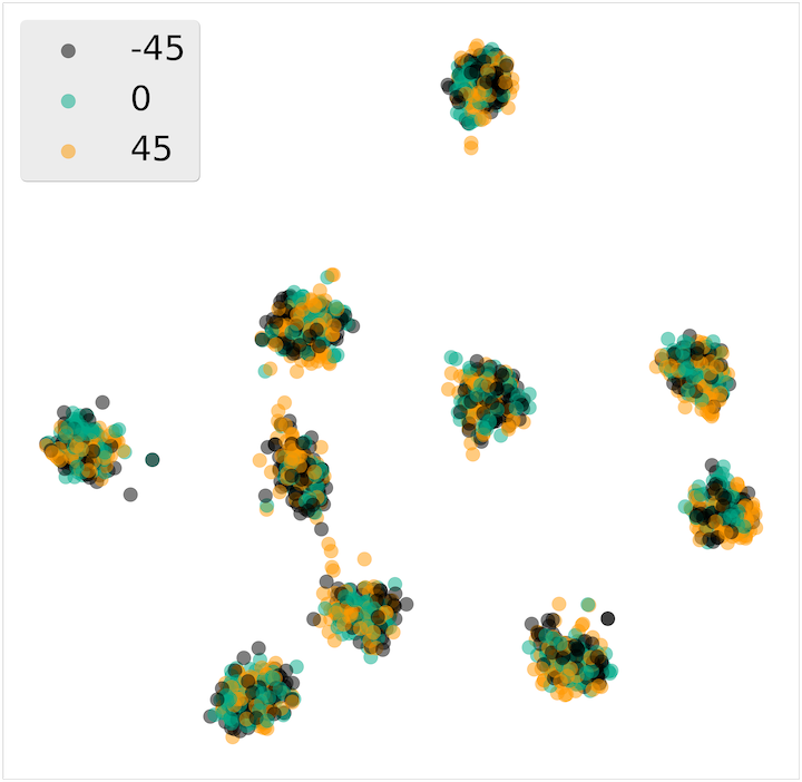
$z_{p}$ embedding

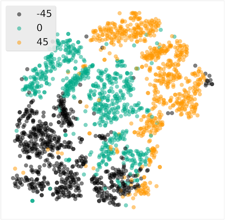
$z_{n}$ embedding

Figure 1: t-SNE visualization of $z_{p}$ and $z_{n}$ embeddings of MNIST-ROT images labeled by rotation angle. As desired, the $z_{p}$ embedding does not encode rotation information, which migrates to $z_{n}$.

We start with rearranging the proposed objective in Equation 3 using the identity from Equation 9 as $I(z_{p}:x)=I(z_{p}:z_{n})+I(z_{p}:x|z_{n})$. This gives us:

$$J =\alpha I(z_{p}:y)+I(x:\{z_{p},z_{n}\})$$

$$\qquad\qquad-\lambda I(z_{p}:x)-\gamma I(z_{p}:z_{n})$$

$$=\alpha I(z_{p}:y)+I(x:\{z_{p},z_{n}\})-\lambda I(z_{p}:z_{n})$$

$$\qquad\qquad-\lambda I(z_{p}:x|z_{n})-\gamma I(z_{p}:z_{n})$$

$$=\alpha I(z_{p}:y)+\Bigl{\{}I(x:\{z_{p},z_{n}\})-\lambda I(z_{p}:x|z_{n})\Bigr{\}}$$

$$\qquad\qquad-(\lambda+\gamma)I(z_{p}:z_{n})$$ (16)

Recall that the chain rule for mutual information in Equation 10 implies that $I(x:\{z_{p},z_{n}\})=I(z_{n}:x)+I(z_{p}:x|z_{n})$. In the expression $I(x:\{z_{p},z_{n}\})-\lambda I(z_{p}:x|z_{n})$ in braces above, our objective simply downweights the $I(z_{p}:x|z_{n})$ component of $I(x:\{z_{p},z_{n}\})$ as:

$$I(x:\{z_{p},z_{n}\})-\lambda I(z_{p}:x|z_{n})$$

$$\qquad\qquad=I(z_{n}:x)+(1-\lambda)I(z_{p}:x|z_{n})$$ (17)

This is equivalent to calculating $I(x:\{\tilde{z}_{p},z_{n}\})$ for a noisified $\tilde{z}_{p}=\psi(z_{p})$ such that:

$$I(x:\{\tilde{z}_{p},z_{n}\}) =I(z_{n}:x)+I(\tilde{z}_{p}:x|z_{n})$$ (18)

$$I(\tilde{z}_{p}:x|z_{n}) =(1-\lambda)I(z_{p}:x|z_{n})$$ (19)

where the free parameter $\lambda$ can be chosen to enforce this relationship. In particular, $\lambda$ depends on $I(z_{p}:x|\{\tilde{z_{p}},z_{n}\})$, which measures the information about $x$ that is destroyed by adding noise through $\psi$. We derive this result using the chain rule for mutual information in two different ways:

$$I(x:\{\tilde{z}_{p},z_{p},z_{n}\})=I(x:\{\tilde{z}_{p},z_{n}\})+I(z_{p}:x|\{\tilde{z}_{p},z_{n}\})$$

$$=I(x:\{z_{p},z_{n}\})+I(\tilde{z}_{p}:x|\{z_{p},z_{n}\})$$

$$\therefore~{}I(x:\{z_{p},z_{n}\})=I(x:\{\tilde{z}_{p},z_{n}\})+I(z_{p}:x|\{\tilde{z}_{p},z_{n}\})$$ (20)

In Equation 20, we used the fact that $I(\tilde{z}_{p}:x|\{z_{p},z_{n}\})=0$ by the data processing inequality. Using the chain rule again, we know that both $I(x:\{z_{p},z_{n}\})$ and $I(x:\{\tilde{z}_{p},z_{n}\})$ contain a $I(z_{n}:x)$ term. Canceling out $I(z_{n}:x)$ and rearranging to match the form of Equation 19, we obtain:

$$I(\tilde{z}_{p}:x|z_{n}) =I(z_{p}:x|z_{n})-I(z_{p}:x|\{\tilde{z}_{p},z_{n}\})$$ (21)

Thus, the information using a noisy $\tilde{z}_{p}$ instead of $z_{p}$ differs by a term of $I(z_{p}:x|\{\tilde{z}_{p},z_{n}\})$. Since $\lambda$ is a free parameter and does not appear elsewhere in the objective, it can be set to satisfy Equation 19. The objective function in Equation 16 can be rewritten with this noisy $\tilde{z}_{p}$ as:

$$J=\alpha I(z_{p}:y)+I(x:\{\tilde{z}_{p},z_{n}\})-\gamma I(z_{p}:z_{n})$$ (22)

Although not explored in (Jaiswal et al.,, 2018), Equation 22 describes an information theoretic formulation of UAI.

Table 1: MNIST-ROT results presented as accuracy for $\Theta=\{0,\pm 22.5,\pm 45\}$ that the models were trained on and unseen $\pm 55$ and $\pm 65$ angles. VFAE could not be evaluated for $\pm 55$ and $\pm 65$ as it uses $s$ as input for encoding $x$ and cannot be used for unseen $s$. The $y$-accuracy should be high but $s$-accuracy should be close to random chance (0.20). RI indicates relative improvement in error-rate between DSF-H (ours) and UAI (previous best).

Acc.	$\bm{\theta}$	VFAE	CAI	CVIB	UAI	DSF-E	DSF-C	DSF-H	RI
$y$	$\Theta$	0.953	0.958	0.960	0.977	0.980	0.981 $\pm$ 0.001	0.981 $\pm$ 0.001	17%
	$\pm$55	$\times$	0.826	0.819	0.856	0.865	0.869 $\pm$ 0.001	0.873 $\pm$ 0.002	12%
	$\pm$65	$\times$	0.662	0.674	0.696	0.707	0.724 $\pm$ 0.002	0.732 $\pm$ 0.001	12%
$s$	$\Theta$	0.389	0.384	0.382	0.338	0.200	0.200 $\pm$ 0.001	0.200 $\pm$ 0.000	100%

Table 2: MNIST-DIL results presented as accuracy for various kernel sizes $\kappa$ (positive for dilation and negative for erosion). Models were trained on MNIST-ROT but tested on MNIST-DIL. RI indicates relative improvement in error-rate between DSF-H (ours) and UAI (previous best).

Acc.	$\bm{\kappa}$	VFAE	CAI	CVIB	UAI	DSF-E	DSF-C	DSF-H	RI
$y$	-2	0.807	0.816	0.844	0.880	0.891	0.899 $\pm$ 0.002	0.907 $\pm$ 0.001	22%
	2	0.916	0.933	0.933	0.958	0.964	0.966 $\pm$ 0.001	0.970 $\pm$ 0.001	28%
	3	0.818	0.795	0.846	0.874	0.887	0.889 $\pm$ 0.002	0.892 $\pm$ 0.002	14%
	4	0.548	0.519	0.586	0.606	0.608	0.608 $\pm$ 0.002	0.610 $\pm$ 0.002	1%

The UAI model uses independent multiplicative Bernoulli noise to create a noisy $\tilde{z}_{p}=\psi(z_{p})$, which is then used alongside $z_{n}$ in a variational decoder maximizing $I(x:\{\tilde{z}_{p},z_{n}\})$. This has the indirect effect of regularizing $I(z_{p}:x)$, since nuisance information cannot be reliably passed through $\tilde{z}_{p}$ for the reconstruction task. In contrast, the proposed objective in Equation 3 directly constrains the information channel between $x$ and $z_{p}$, which guarantees invariance to nuisance at optimality (Achille and Soatto, 2018a, ).

5 Experimental Evaluation

Empirical results are presented on four datasets — MNIST-ROT (Jaiswal et al.,, 2018), MNIST-DIL (Jaiswal et al.,, 2018), Multi-PIE (Gross et al.,, 2008), and Chairs (Aubry et al.,, 2014), following previous works (Li et al.,, 2014; Louizos et al.,, 2016; Moyer et al.,, 2018; Xie et al.,, 2017; Jaiswal et al.,, 2018). Samples of images in these datasets are shown in the supplementary material. The proposed model is compared with previous state-of-the-art: VFAE, CAI, CVIB, and UAI. Results are also reported for an ablation version of our framework, DSF-E, which models the IB objective in Equation 1. We optimize an exact expression for $I(z_{p}:x)$, as presented in Section 3.2, for DSF-E. Hence, we do not evaluate methods that are similar to the ablation model but indirectly optimize $I(z_{p}:x)$ (Achille and Soatto, 2018b, ; Alemi et al.,, 2016).

The accuracy of predicting $y$ from $z_{p}$ is reported for the trained models. Additionally, the accuracy of predicting $s$ is reported as a measure of invariance using two layer neural networks that were trained post hoc to predict known $s$ from $z_{p}$, following previous works (Jaiswal et al.,, 2018; Moyer et al.,, 2018). While the $y$-accuracy is desired to be high, the $s$-accuracy should be close to random chance of $s$ for true invariance. Results of the full version of our model are reported as mean and standard-deviation based on five runs. We also report relative improvements (%) in error-rate over previous best models. The error-rate for $s$ is calculated as the difference between $s$-accuracy and random chance. Furthermore, t-SNE (Maaten and Hinton,, 2008) visualization of the $z_{p}$ and $z_{n}$ embeddings are presented for the DSF-H version of the proposed model for visualizing the separation of nuisance factors.

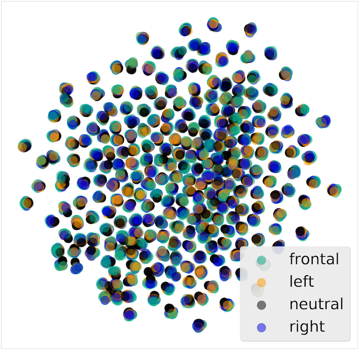
$z_{p}$ – labeled by illumination

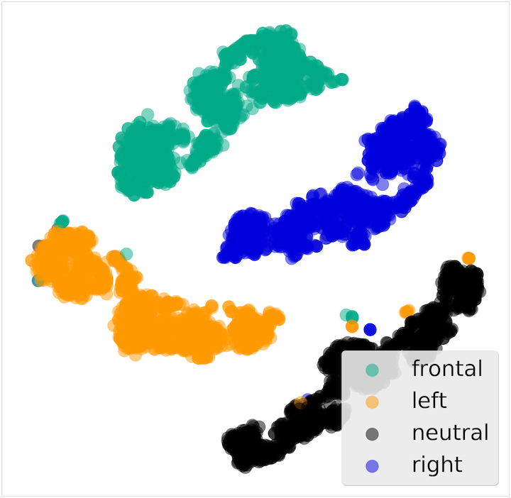
$z_{n}$ – labeled by illumination

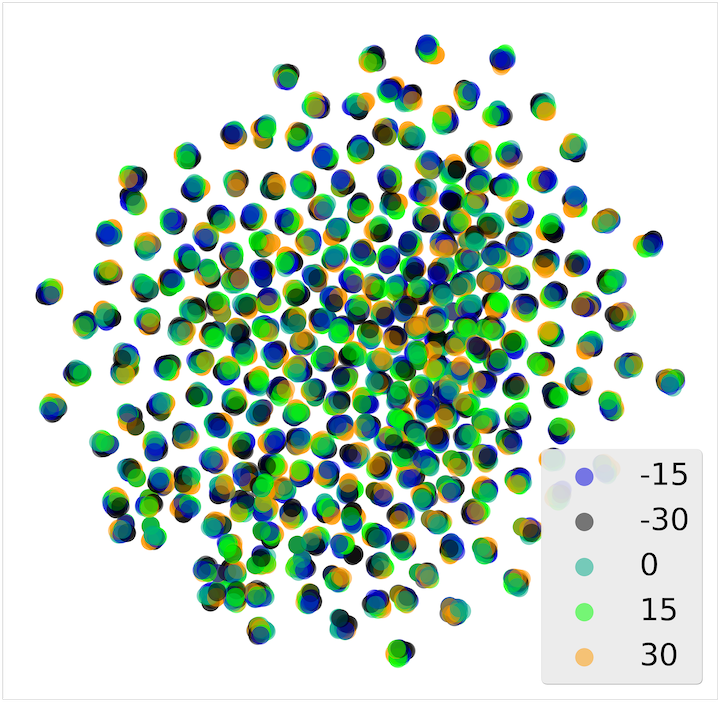
$z_{p}$ – labeled by pose

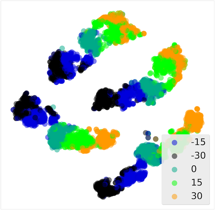
$z_{n}$ – labeled by pose

Figure 2: t-SNE visualization of $z_{p}$ and $z_{n}$ embeddings of Multi-PIE images labeled by illumination (top row) and pose (bottom row). As desired, $z_{p}$ does not encode illumination and pose, both of which migrate to $z_{n}$.

Table 3: Multi-PIE — $y$-accuracy should be high but $s$-accuracy should be random chance (illumination (i): 0.25, pose (p): 0.20). Separate models were trained for illumination and pose for previous supervised invariance methods: VFAE, CAI, and CVIB. RI indicates relative improvement in error-rate over previous best (UAI).

Acc.	VFAE		CAI		CVIB		UAI	DSF-E	DSF-C	DSF-H	RI
	$s$: i	$s$: p	$s$: i	$s$: p	$s$: i	$s$: p
$y$	0.67	0.62	0.76	0.77	0.51	0.46	0.82	0.83	0.85 $\pm$ 0.00	0.87 $\pm$ 0.01	28%
$s$: i	0.41	0.80	0.99	1.00	0.44	0.63	0.61	0.25	0.25 $\pm$ 0.02	0.25 $\pm$ 0.00	100%
$s$: p	0.65	0.29	0.98	0.98	0.45	0.28	0.32	0.20	0.20 $\pm$ 0.01	0.20 $\pm$ 0.00	100%

Table 4: Chairs results — $y$-accuracy should be high but $s$-accuracy should be random chance (0.25). RI indicates relative improvement in error-rate between DSF-H (ours) and UAI (previous best).

Acc.	VFAE	CAI	CVIB	UAI	DSF-E	DSF-C	DSF-H	RI
$y$	0.72	0.68	0.67	0.74	0.84	0.86 $\pm$ 0.01	0.88 $\pm$ 0.01	54%
$s$	0.37	0.69	0.52	0.34	0.25	0.25 $\pm$ 0.00	0.25 $\pm$ 0.00	100%

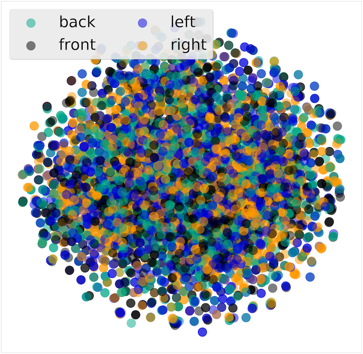
$z_{p}$ embedding

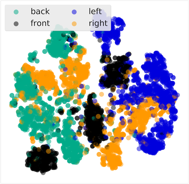
$z_{n}$ embedding

Figure 3: t-SNE visualization of $z_{p}$ and $z_{n}$ embeddings of Chairs images labeled by yaw orientation. As desired, the $z_{p}$ embedding does not encode orientation information, which migrates to $z_{n}$.

MNIST-ROT: This dataset was introduced in (Jaiswal et al.,, 2018) as an augmented version of the MNIST (LeCun et al.,, 1998) dataset that contains digits rotated at angles $\theta\in\Theta=\{0,\pm 22.5,\pm 45\}$ for training. Evaluation is performed on digits rotated at $\theta\in\Theta$ as well as for $\pm 55$ and $\pm 65$. We use the same version of the dataset as (Jaiswal et al.,, 2018). The NN instantiation of the proposed model also follows UAI with two layers for encoding $x$ into $z_{p}$ and $z_{n}$, two layers for inferring $y$ from $z_{p}$, and three layers for reconstructing $x$ from $\{z_{p},z_{n}\}$. The digit class is treated as $y$ and categorical $\theta$ as $s$. Table 1 presents results of our dataset, showing that all versions of the proposed framework outperform previous state-of-the-art models with DSF-H achieving the best $y$-accuracies. Furthermore, without using $s$-labels, all versions of the proposed framework achieve random chance $s$-accuracy ($0.20$), which indicates perfect invariance to rotation angle. Figure 1 shows the t-SNE visualization of $z_{p}$ and $z_{n}$. As evident, $z_{p}$ does not cluster by rotation angle but $z_{n}$ does, which validates that this nuisance factor is separated out and encoded in $z_{n}$ instead of $z_{p}$.

MNIST-DIL: This variant of MNIST contains digits eroded or dilated with various kernel sizes $\kappa\in\{-2,2,3,4\}$, as introduced in (Jaiswal et al.,, 2018). MNIST-DIL is used for further evaluating models trained on the MNIST-ROT dataset for varying stroke-widths, which is not explicitly controlled in MNIST-ROT but is implicitly present. Results in Table 2 show that all versions of the proposed framework outperform previous works by retaining more predictive information in $z_{p}$.

Multi-PIE: This is a dataset of face images of 337 subjects captured at 15 poses and 19 illumination conditions with various facial expressions. A subset of the data is prepared for this experiment that contains 264 subjects with images captured at five pose angles $\{0,\pm 15,\pm 30\}$ and four illumination conditions: neutral, frontal, left, and right. The subject identity is treated as $y$ while pose and illumination are treated as nuisances. The NN instantiation of the proposed model uses one layer each for encoding $z_{p}$ and $z_{n}$, and for predicting $y$ from $z_{p}$, while two layers are used for reconstructing $x$ from $\{z_{p},z_{n}\}$. Table 3 presents the results of this experiment, showing that all versions of the proposed model outperform previous works on both $y$-accuracy and $s$-accuracy of both illumination and pose. The t-SNE visualization of $z_{p}$ and $z_{n}$ in Figure 2 shows that both illumination and pose information are separated out and encoded in $z_{n}$ instead of $z_{p}$, resulting in an invariant $z_{p}$ embedding.

Chairs: This dataset contains images of chairs at various yaw angles, which are binned into four orientations: front, back, left, and right. We use the same version of this dataset as (Jaiswal et al.,, 2018) where the yaw angles do not overlap between the train and test sets. The NN instantiation follows (Jaiswal et al.,, 2018) with two layers each for encoding $z_{p}$ and $z_{n}$ from $x$, predicting $y$ from $z_{p}$, and reconstructing $x$ from $\{z_{p},z_{n}\}$. Results are summarized in Table 4, showing that all versions of the proposed framework outperform previous methods by a large margin on both $y$-accuracy and $s$-accuracy. All versions of the proposed framework also achieve random chance $s$-accuracy ($0.25$), which indicates perfect invariance to orientation, without using $s$-labels during training. Figure 3 shows the t-SNE visualization of $z_{p}$ and $z_{n}$, further validating that the orientation information is separated out of $z_{p}$ and encoded in $z_{n}$.

6 Conclusion

We have presented a novel framework for inducing nuisance-invariant representations in supervised NNs through learning to encode all information about the data while separating out predictive and nuisance factors into independent embeddings. We provided an information theoretic formulation of the approach and derived training objectives from it. Furthermore, we provided a theoretical analysis of the proposed model and derived a connection with the UAI model, showing that the proposed framework is superior to UAI. Empirical results on benchmark datasets show that the proposed framework outperforms previous works with large relative improvements.

References

- (1) Achille, A. and Soatto, S. (2018a). Emergence of invariance and disentanglement in deep representations. Journal of Machine Learning Research, 19(50):1–34.
- (2) Achille, A. and Soatto, S. (2018b). Information dropout: Learning optimal representations through noisy computation. IEEE Transactions on Pattern Analysis and Machine Intelligence, 40(12):2897–2905.
- Alemi et al., (2016) Alemi, A. A., Fischer, I., Dillon, J. V., and Murphy, K. (2016). Deep variational information bottleneck. arXiv preprint arXiv:1612.00410.
- Aubry et al., (2014) Aubry, M., Maturana, D., Efros, A., C. Russell, B., and Sivic, J. (2014). Seeing 3d chairs: Exemplar part-based 2d-3d alignment using a large dataset of cad models. In Proceedings of the IEEE Computer Society Conference on Computer Vision and Pattern Recognition.
- Brekelmans et al., (2019) Brekelmans, R., Moyer, D., Galstyan, A., and Steeg, G. V. (2019). Exact rate-distortion in autoencoders via echo noise. arXiv preprint arXiv:1904.07199.
- Ganin et al., (2016) Ganin, Y., Ustinova, E., Ajakan, H., Germain, P., Larochelle, H., Laviolette, F., Marchand, M., and Lempitsky, V. (2016). Domain-adversarial training of neural networks. The Journal of Machine Learning Research, 17(1):2096–2030.
- Gao et al., (2016) Gao, S., Ver Steeg, G., and Galstyan, A. (2016). Variational information maximization for feature selection. In Advances in neural information processing systems, pages 487–495.
- Gretton et al., (2007) Gretton, A., Borgwardt, K. M., Rasch, M., Schölkopf, B., and Smola, A. J. (2007). A kernel method for the two-sample-problem. In Schölkopf, B., Platt, J. C., and Hoffman, T., editors, Advances in Neural Information Processing Systems 19, pages 513–520. MIT Press.
- Gretton et al., (2005) Gretton, A., Bousquet, O., Smola, A., and Schölkopf, B. (2005). Measuring statistical dependence with hilbert-schmidt norms. In Jain, S., Simon, H. U., and Tomita, E., editors, Algorithmic Learning Theory, pages 63–77, Berlin, Heidelberg. Springer Berlin Heidelberg.
- Gross et al., (2008) Gross, R., Matthews, I., Cohn, J., Kanade, T., and Baker, S. (2008). Multi-pie. In 2008 8th IEEE International Conference on Automatic Face Gesture Recognition, pages 1–8.
- Hsu et al., (2019) Hsu, I.-H., Jaiswal, A., and Natarajan, P. (2019). Niesr: Nuisance invariant end-to-end speech recognition. Proceedings of Interspeech 2019, pages 456–460.
- Jaiswal et al., (2020) Jaiswal, A., Moyer, D., Steeg, G. V., AbdAlmageed, W., and Natarajan, P. (2020). Invariant representations through adversarial forgetting. In Proceedings of the AAAI Conference on Artificial Intelligence, volume 34.
- Jaiswal et al., (2018) Jaiswal, A., Wu, R. Y., Abd-Almageed, W., and Natarajan, P. (2018). Unsupervised adversarial invariance. In Bengio, S., Wallach, H., Larochelle, H., Grauman, K., Cesa-Bianchi, N., and Garnett, R., editors, Advances in Neural Information Processing Systems 31, pages 5097–5107. Curran Associates, Inc.
- (14) Jaiswal, A., Wu, Y., AbdAlmageed, W., and Natarajan, P. (2019a). Unified Adversarial Invariance. arXiv preprint arXiv:1905.03629.
- (15) Jaiswal, A., Xia, S., Masi, I., and AbdAlmageed, W. (2019b). RoPAD: Robust Presentation Attack Detection through Unsupervised Adversarial Invariance. In 12th IAPR International Conference on Biometrics (ICB).
- Ko et al., (2015) Ko, T., Peddinti, V., Povey, D., and Khudanpur, S. (2015). Audio augmentation for speech recognition. In Sixteenth Annual Conference of the International Speech Communication Association.
- Krizhevsky et al., (2012) Krizhevsky, A., Sutskever, I., and Hinton, G. E. (2012). Imagenet classification with deep convolutional neural networks. In Advances in neural information processing systems, pages 1097–1105.
- Lample et al., (2017) Lample, G., Zeghidour, N., Usunier, N., Bordes, A., DENOYER, L., et al. (2017). Fader networks: Manipulating images by sliding attributes. In Advances in Neural Information Processing Systems, pages 5963–5972.
- LeCun et al., (1998) LeCun, Y., Bottou, L., Bengio, Y., and Haffner, P. (1998). Gradient-based Learning Applied to Document Recognition. Proceedings of the IEEE, 86(11):2278–2324.
- Li et al., (2014) Li, Y., Swersky, K., and Zemel, R. (2014). Learning unbiased features. arXiv preprint arXiv:1412.5244.
- Lopez et al., (2018) Lopez, R., Regier, J., Jordan, M. I., and Yosef, N. (2018). Information constraints on auto-encoding variational bayes. In Bengio, S., Wallach, H., Larochelle, H., Grauman, K., Cesa-Bianchi, N., and Garnett, R., editors, Advances in Neural Information Processing Systems 31, pages 6117–6128. Curran Associates, Inc.
- Louizos et al., (2016) Louizos, C., Swersky, K., Li, Y., Welling, M., and Zeme, R. (2016). The variational fair autoencoder. In Proceedings of International Conference on Learning Representations.
- Maaten and Hinton, (2008) Maaten, L. v. d. and Hinton, G. (2008). Visualizing data using t-sne. Journal of machine learning research, 9(Nov):2579–2605.
- Miao and Niu, (2016) Miao, J. and Niu, L. (2016). A survey on feature selection. Procedia Computer Science, 91:919 – 926. Promoting Business Analytics and Quantitative Management of Technology: 4th International Conference on Information Technology and Quantitative Management (ITQM 2016).
- Moyer et al., (2018) Moyer, D., Gao, S., Brekelmans, R., Galstyan, A., and Ver Steeg, G. (2018). Invariant representations without adversarial training. In Bengio, S., Wallach, H., Larochelle, H., Grauman, K., Cesa-Bianchi, N., and Garnett, R., editors, Advances in Neural Information Processing Systems 31, pages 9102–9111. Curran Associates, Inc.
- Sabour et al., (2017) Sabour, S., Frosst, N., and Hinton, G. E. (2017). Dynamic routing between capsules. In Advances in Neural Information Processing Systems, pages 3859–3869.
- Tishby et al., (1999) Tishby, N., Pereira, F. C., and Bialek, W. (1999). The information bottleneck method. In 37th Annual Allerton Conference on Communication, Control and Computing, pages 368–377.
- Xie et al., (2017) Xie, Q., Dai, Z., Du, Y., Hovy, E., and Neubig, G. (2017). Controllable invariance through adversarial feature learning. In Guyon, I., Luxburg, U. V., Bengio, S., Wallach, H., Fergus, R., Vishwanathan, S., and Garnett, R., editors, Advances in Neural Information Processing Systems 30, pages 585–596. Curran Associates, Inc.
- Zemel et al., (2013) Zemel, R., Wu, Y., Swersky, K., Pitassi, T., and Dwork, C. (2013). Learning fair representations. In Dasgupta, S. and McAllester, D., editors, Proceedings of the 30th International Conference on Machine Learning, volume 28 of Proceedings of Machine Learning Research, pages 325–333, Atlanta, Georgia, USA. PMLR.
- Zhang et al., (2016) Zhang, Y., Lee, K., and Lee, H. (2016). Augmenting supervised neural networks with unsupervised objectives for large-scale image classification. In International Conference on Machine Learning, pages 612–621.