Identifying nearby sources of ultra-high-energy cosmic rays with deep learning

Abstract

We present a method to analyse arrival directions of ultra-high-energy cosmic rays (UHECRs) using a classifier defined by a deep convolutional neural network trained on a HEALPix grid. To illustrate a high effectiveness of the method, we employ it to estimate prospects of detecting a large-scale anisotropy of UHECRs induced by a nearby source with an (orbital) detector having a uniform exposure of the celestial sphere and compare the results with our earlier calculations based on the angular power spectrum. A minimal model for extragalactic cosmic rays and neutrinos by Kachelrieß, Kalashev, Ostapchenko and Semikoz (2017) is assumed for definiteness and nearby active galactic nuclei Centaurus A, M82, NGC 253, M87 and Fornax A are considered as possible sources of UHECRs. We demonstrate that the proposed method drastically improves sensitivity of an experiment by decreasing the minimal required amount of detected UHECRs or the minimal detectable fraction of from-source events several times compared to the approach based on the angular power spectrum. We also test robustness of the neural networks against different models of the large-scale Galactic magnetic fields and variations of the mass composition of UHECRs, and consider situations when there are two nearby sources or the dominating source is not known a priori. In all cases, the neural networks demonstrate good performance unless the test models strongly deviate from those used for training. The method can be readily applied to the analysis of data of the Telescope Array, the Pierre Auger Observatory and other cosmic ray experiments.

1 Introduction

Cosmic rays of the highest energies ($E\gtrsim 50$ EeV, ultra-high-energy cosmic rays, UHECRs) were first detected almost 60 years ago [1] and still remain at the forefront of the high-energy astrophysics. Due to the limited distance of CR propagation at these energies amounting to $\sim$100 Mpc, a certain degree of anisotropy is expected in the distribution of their arrival directions. The level of an anisotropy and its other properties depend on characteristics of sources of UHECRs, thus studying the anisotropy is one of the key parts of this branch of astrophysics.

An analysis of an anisotropy of CR arrival directions is only feasible when a sufficiently large amount of data is available. Due to the extremely low flux of UHECRs, obtaining the required number of events demands instruments with a very large exposure. One of possible solutions of the problem is employing space-born detectors, which observe UV-radiation from extensive air showers induced by UHECRs in the Earth’s atmosphere. Several missions of the kind are under development now, such as KLYPVE-EUSO (K-EUSO) [2, 3, 4, 5] and POEMMA [6, 7]. In our previous paper [8] (Paper 1 in what follows), we studied sensitivity of these future orbital missions to a large-scale anisotropy emerging due to the presence of a nearby source. A particular model for cosmic rays and neutrinos by Kachelrieß, Kalashev, Ostapchenko and Semikoz (KKOS in what follows) [9], which can act as a representative of a broader class of models, was selected for the analysis. The model assumes that UHECRs are accelerated by (a subclass of) active galactic nuclei (AGN) with the energy spectra of nuclei following a power-law with a rigidity-dependent cut-off after the acceleration phase. The model successfully reproduces the energy spectrum of cosmic rays with energies beyond $10^{17}$ eV registered with the Pierre Auger Observatory and the spectrum of high-energy neutrinos registered by IceCube, as well as data on the depth of maximum of air showers $X_{\mathrm{max}}$ and RMS($X_{\mathrm{max}}$). One of the consequences of the model is the existence of a nearby (within $\sim 20$ Mpc) AGN acting as a source of UHECRs. Presence of such an accelerator would inevitably lead to deviations from isotropy at some level and produce detectable imprints on the angular power spectrum (APS) of the UHECR flux providing the fraction of nuclei arriving from the source is sufficiently high. We considered five nearby AGN often discussed in literature as possible sources of UHECRs and demonstrated that an observation of $\gtrsim 200\text{--}300$ events with energies $\gtrsim 57$ EeV will allow detecting deviations from isotropy with a high level of statistical significance if the fraction of events from any of these sources is $\simeq$10–15% of the total flux.

Use of the APS allows for a very robust approach to an analysis of anisotropy but has certain drawbacks since some information such as the characteristic shape and size of a region with an excessive flux of UHECRs produced by the source is only partially preserved in the APS coefficients. That results in a somewhat lower sensitivity to a sought signal. In the present paper, we searched for this signal exploiting information about arrival directions of UHECRs. To do that, we employed a convolutional neural network (CNN) classifier. It is known that CNNs have demonstrated high performance in a wide range of problems related to classification of data and pattern recognition, see, e.g., [10]. However, to the best of our knowledge, they have never been employed for anisotropy studies in UHECR physics yet.

In what follows, we present a CNN trained on a HEALPix grid [11] and demonstrate that it presents a real breakthrough by reducing the number of events needed for establishing a large-scale anisotropy produced by UHECRs arriving from a nearby source by $\sim 4$ times. Alternatively, for a fixed sample size, the CNN strongly decreases the fraction of CRs arriving from the source necessary for a robust detection of an anisotropy.

2 Traditional approach

Let us briefly remind the key points of Paper 1, which was based on calculating the angular power spectrum of CR arrival directions mostly following a method suggested by the IceCube and the Pierre Auger Observatory collaborations [12, 13]. We considered five nearby active galactic nuclei Centaurus A, M82, NGC 253, M87 and Fornax A as possible sources of UHECRs. All of them are located within a sphere with a radius of $\sim 20$ Mpc with the first three being as close as $\approx 3.5\text{--}4$ Mpc from the Galaxy. For the aims of the analysis, we generated multiple sets of mock maps imitating arrival directions of nuclei coming from these sources.

In a simplified approach of the KKOS model, all sources share the same injection spectrum and composition. These properties were found from the global fit of the CR spectrum and composition observed at Earth. However, both composition and spectrum evolve during propagation of nuclei in the inter-galactic media. That was taken into account with the TransportCR code [14]. We only considered nuclei with energies above 57 EeV, which approximately corresponds to the 100% efficiency threshold of the K-EUSO and POEMMA projects. This allowed us to assume that extragalactic magnetic fields do not strongly deflect the nuclei [15] so that UHECRs arrive to the Milky Way within $\pm 1^{\circ}$ from the original direction. Next, we employed the CRPropa 3 code [16] to simulate propagation of nuclei in the Galactic magnetic field (GMF), for which we assumed the Jansson–Farrar model [17, 18], JF12 in what follows. All three components of the magnetic field present in the model (the regular, striated and turbulent ones) were utilised in simulations. The calculations were performed on the HEALPix grid with $N_{\mathrm{side}}=512$. The corresponding angular resolution of the grid ($7^{\prime}$) is much higher than the angular resolution of any of the existing or forthcoming cosmic ray experiments but it allowed us to obtain an accurate sampling of arrival directions of from-source UHECRs.

Having these tools, it is straightforward to produce a map of arrival directions of $N$ UHECRs, $N_{\mathrm{src}}$ of which come from a particular source. The procedure is as follows. One takes the propagated spectrum calculated with TransportCR for a source located at a given distance from the Galaxy and samples it $N_{\mathrm{src}}$ times, each time extracting some nuclei with an energy $E$ and charge $Z$. An observed arrival direction of a cosmic ray is found then for each $(E,Z)$ pair (or, equivalently, for each rigidity) using the mapping obtained with CRPropa by backpropagation. Finally, the remaining $N-N_{\mathrm{src}}$ events are generated following the isotropic distribution. The whole process is repeated multiple times in order to generate a large number of maps for each source.

After that, we prepared maps of the relative intensity of the CR flux and calculated their angular power spectra looking for the minimal fraction $\eta$ of from-source events in the whole sample allowing one to reject the null hypothesis of an isotropic distribution at a high confidence level. The hypothesis of isotropy was tested using the following estimator:

$$D(\text{sample})=\frac{1}{\ell_{\mathrm{max}}}\sum_{\ell=1}^{\ell_{\mathrm{max}}}\frac{C_{\ell,\mathrm{sample}}-\langle C_{\ell,\mathrm{iso}}\rangle}{\sigma_{\ell,\mathrm{iso}}},$$ (2.1)

where “sample” is either “mix” when applied to samples that contain a contribution from an UHECR source, or “iso” when applied to isotropic samples, and $C_{\ell}$ are coefficients of the angular power spectrum:

$$C_{\ell}=\frac{1}{2\ell+1}\sum_{m=-\ell}^{+\ell}|a_{\ell m}|^{2}.$$ (2.2)

Thus, variables $C_{\ell,\mathrm{sample}}$, $\langle C_{\ell,\mathrm{iso}}\rangle$ and $\sigma_{\ell,\mathrm{iso}}$ in eq. (2.1) are respectively the $C_{\ell}$ observed in the sample (either “mix” or “iso”), the average and the standard deviation of $C_{\ell}$ for isotropic expectations, all of them calculated at a given scale $\ell$. Coefficients $a_{\ell m}$ in eq. (2.2) are the multipolar moments of the spherical harmonics used to decompose the relative intensity of the flux.

Since both $D(\mathrm{iso})$ and $D(\mathrm{mix})$ in eq. (2.1) are random variables, one needs to compare their distributions. It was assumed as the null hypothesis $H_{0}$ that arrival directions of a mixed sample of UHECRs obey an isotropic distribution. We adopted the value of the error of the second kind (the probability not to reject the null hypothesis when it is false) $\beta=0.05$ and searched for a minimal fraction $\eta$ of from-source events in the total flux such that the error of the first kind (the probability to reject the true null hypothesis) $\alpha\lesssim 0.01$. For the sake of uniformity, all calculations of the estimator $D$ in Paper 1 were done with $\ell_{\mathrm{max}}=16$ though it was remarked that the choice is not necessarily optimal, and slightly better results can be obtained by adjusting $\ell_{\mathrm{max}}$ for each particular source, depending on its angular power spectrum.

We used samples of sizes $N=100,200,\dots,500$ to cover the whole possible range of UHECRs to be detected by K-EUSO above 57 EeV [4]. It was demonstrated that an observation of $\gtrsim 200\text{--}300$ events over the celestial sphere (depending on the particular source) will allow testing $H_{0}$ with the above demands on $\alpha$ and $\beta$ providing the from-source events form 10–15% of the total sample. In other words, registering a sample of that size will allow one to detect a large-scale anisotropy arising due to a nearby source with a high confidence level.

Adjusting $\ell_{\mathrm{max}}$ to minimize $\eta$ allows one to decrease numbers obtained with the APS method by a few percent (from 2–5% for $N=100$ to 1–2% for $N=500$) most notably for Cen A and Fornax A, for which a deviation of the lower multipoles from the isotropic distribution is most pronounced, see Paper 1. Obviously, this does not present a noticeable improvement of the result.

We remark the KKOS model provides a heavy mass composition of UHECRs at energies above 57 EeV thus resulting in much more fuzzy patterns of arrival directions if compared with the case of a light (mostly proton and helium) composition. In this sense, our results are conservative since having more compact patterns will allow obtaining less restrictive demands on the minimal number of from-source events needed to reject the isotropy hypothesis.

3 Deep convolutional classifier

As we have already mentioned above, a test statistics based solely on the angular power spectrum cannot benefit from information about a pattern of arrival directions of UHECRs coming from a particular source. An obvious way to overcome this limitation is to use some function of the expected and observed arrival direction maps. In what follows, we use a classifier based on the convolutional neural network architecture as a test statistics. Recall that CNNs present a widely used subclass of feed-forward neural networks designed specifically for pattern recognition and image classification tasks [19].

The basic idea behind CNNs is using local feature maps at different scales to extract valuable information and perform a classification task. A variety of CNN implementations exist for many programming languages and platforms. However, most of them support operations on flat (two-dimensional) images only. A number of implementations for convolutional operations on the sphere were proposed recently [20, 21, 22]. We employed the publicly available code developed by Krachmalnicoff and Tomasi [22], which implements convolution and pooling (down-sampling) operations on the HEALPix grid data with the help of Keras deep learning library [24]. The convolution operation on the HEALPix grid is parameterized by 9 adjustable weights per feature map. The CNN architecture developed in this work is shown in figure 1.

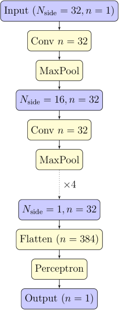
Figure 1: Architecture of the CNN developed in this work. Blue boxes are used to show feature vectors and maps. Yellow boxes show operations.

The network takes one feature map ($n=1$ in figure 1) in the HEALPix grid with $N_{\mathrm{side}}=32$ as an input. Thirty-two feature maps ($n=32$) are built at the first step using the convolution operation with $32\times 9$ free parameters and max-pooling the image to $N_{\mathrm{side}}=16$. The sequence of convolutions and max-pooling operations is repeated until reaching $N_{\mathrm{side}}=1$ with the persistent number of feature maps, which means that each intermediate convolution operation has $32\times 32\times 9$ trainable weights. The rectified linear activation function (ReLU) is used for all intermediate layers. Finally, 32 feature maps with $N_{\mathrm{side}}=1$ are flattened and sent to a single-layer sigmoid perceptron. To avoid overfitting, we use an early-stop technique. Namely, we train our model for at most 1000 epochs and interrupt training in case accuracy on validation data is not improving for 10 epochs. Attempts to use other regularization techniques, such as dropout and the L2 regularization demonstrated little benefit. The weights were optimized using the Adadelta adaptive learning rate method [25]. The output of the classifier, a number between 0 and 1 was used as the test statistic. The minimal fractions $\eta$ of from-source UHECRs needed to reject the null hypothesis of an isotropic flux with the same demands on $\alpha$ and $\beta$ as above, are presented in table 1. Results obtained in Paper 1 are included for comparison (for $N\geq 100$). Figure 2 provides two examples of the dependence of the test power $1-\beta$ on the fraction of UHECRs arriving from M 87 for both approaches, two sample sizes and $\alpha=0.01,0.001$. One can clearly see that the CNNs outperform the APS-based approach in terms of the test power for any $\eta$ and $\alpha$.

Table 1: Percentage of UHECRs arriving from the candidate sources in samples of sizes $N=50,100,\dots,500$ such that the error of the first kind $\alpha\lesssim 0.01$ for the null hypothesis of isotropy $H_{0}$ providing the second kind error $\beta=0.05$, obtained with the traditional approach based on the angular power spectrum (APS) and with the convolutional neural network (CNN) shown in figure 1. The result based on the APS was obtained for fixed $\ell_{\mathrm{max}}=16$. One source at a time was considered.

Source	Method	50	100	200	300	400	500
NGC 253	APS	24	17	12	10	8	7
	CNN	12	7	4.5	3.67	3	2.6
Cen A	APS	28	21	14	12	10	9
	CNN	16	11	7	5.67	5	4.4
M 82	APS	36	26	18	14	12	11
	CNN	20	12	7	6	4.75	4.2
M 87	APS	38	29	20	16	14	12
	CNN	22	14	9	8	6.25	5.2
Fornax A	APS	28	19	13	11	9	8
	CNN	16	9	6	5	4.5	3.8

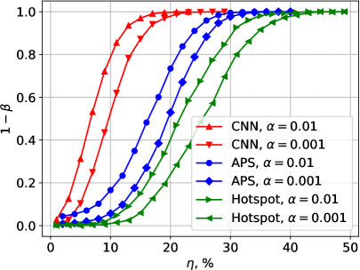
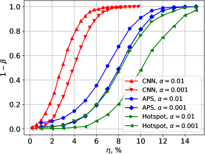
Figure 2: Dependence of the test power $1-\beta$ on the fraction $\eta$ of UHECRs coming from M 87 in samples of size 100 (left) and 500 (right) for the approach based APS (blue) and with the suggested CNN (red) for $\alpha=0.01,0.001$. Green lines show the same for the approach based on a search for a “hotspot” at intermediate angular scales, see Remark 1.

Remark 1.

One might expect that an anisotropy arising due to an impact of a nearby source can be found more effectively with a traditional method similar to the one used for finding the famous “hotspot” discovered by the Telescope Array experiment [26] and other intermediate scale anisotropies found by other experiments. To verify the conjecture, we have written a dedicated code and performed searches for a hotspot taking M 87 as a source for two “limiting” cases, $N=100$ and $N=500$ events, for definiteness. Fraction of from-source events varied in intervals 0–50% and 0–15% in the first and the second cases respectively. We have searched for an excess in circles with radii from 20^∘ to 60^∘ in 10^∘ steps. The results are shown in figure 2 in green. It can be seen that the hotspot approach fared a bit worse than the one based on the APS and was much less sensitive than the CNN. Thus, the approach is not necessary the best in all possible cases though it can definitely be very efficient in certain tasks. A comprehensive investigation of anisotropies at small and intermediate angular scales can be a subject of a separate study.

Notice the minimal fractions of from-source events needed to find an anisotropy with CNNs decreased drastically in comparison with those obtained with the classical approach. Consider for example M 87, which poses the most complicated case in comparison with the other sources due to the fuzzy pattern of UHECR arrival directions, see the right panel of figure 3 and plots in Paper 1. In the classical approach, one needed to register 400 events over the celestial sphere to verify $H_{0}$ for the given restrictions on $\alpha$ and $\beta$, providing the flux of UHECRs arriving from M 87 comprises 14% of the total. With the CNN, one needs to register only 100 events over the sphere to test the hypothesis under the same conditions. This means even a pattern like the one shown in the left panel of figure 3 with 14 UHECRs coming from M 87 and 86 forming the isotropic background allows testing $H_{0}$ by the CNN.

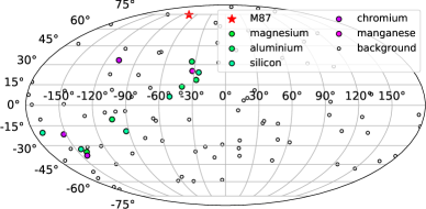
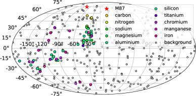
Figure 3: Left: an example of 14 UHECRs with energies above 57 EeV coming from M 87 on the background of 86 events distributed isotropically (i.e., 14% in the sample of 100). A sample like this allows testing $H_{0}$ with the CNN. Right: an example of a sample with the same percentage of UHECRs coming from M 87 (14%) that allows testing $H_{0}$ in the classical approach based on the APS. Here, the total size of the sample equals 400, cf. table 1. The maps are in the Mollweide projection with galactic coordinates.

The situation is similar for the other sources. Notice one needs to register less than 100 events over the whole celestial sphere to verify the null hypothesis providing any of the sources generates $\sim$10–15% of the total flux. Alternatively, given a sample of a fixed size, one will be able to test $H_{0}$ with the CNN with a contribution from a source that it is at least two times less than the one needed in the APS-based approach.

We also tried to use maps with cells of other sizes for the classifier input but found that the minimal fraction of from-source events necessary to test $H_{0}$ only moderately depends on $N_{\mathrm{side}}$ for $N_{\mathrm{side}}\geq 32$ but grows substantially for maps with $N_{\mathrm{side}}\leq 16$.

Remark 2.

It was considered in Paper 1 if an anisotropy arising from a nearby source at energies above 57 EeV can be found by the existing experiments at lower energies. It was demonstrated that a source providing 10–15% of the flux beyond 57 EeV can only contribute 1–1.5% at energies above 8 EeV, at which a dipole anisotropy was found by the Pierre Auger collaboration [27], and there is very little difference between sources located at distances 3.5 Mpc and 20 Mpc in this respect. The approach based on the angular power spectrum and the estimator $D$ defined in eq. (2.1) did not allow us to find an anisotropy from a nearby source even in case the total sample contains 50,000 events, which is close to the size of the Pierre Auger data set taking into account their field of view. To the contrary, the CNN presented above is able to distinguish a pattern of from-source events comprising a much smaller fraction. For example, it is able to verify $H_{0}$ with a pattern produced by UHECRs with energies above 8 EeV coming from Cen A if they constitute as little as $\sim 1\%$ of a sample of that size, with the same cuts on $\alpha$ and $\beta$. This suggests applying the technique to the analysis of data of the existing experiments.

4 Model dependence. Towards a unified test statistic

One of disadvantages of the neural network approach is the resulting model opaqueness. Features used by the trained classifier are hard to extract and interpret. By this reason, it is important to check the test statistic resistance to variations of the physical model assumed during training the neural network. In this section, we present results of this study and propose some ways to make the test statistic more universal. We also consider more realistic cases than the one discussed above, namely, a situation when the source is not known a priori and when there are more than one nearby source contributing to the UHECR flux and generating a kind of anisotropy.

4.1 Galactic magnetic field model uncertainties

As it was mentioned in section 2, the JF12 model of the large-scale Galactic magnetic field [17, 18] was used for training the neural networks presented above, as well as within the traditional approach employed in Paper 1. However, the GMF is not known accurately yet, and some modifications of the JF12 model have been suggested, as well as a number of alternative models. We have considered four recent models for the large-scale GMF, namely, the JF12 model as modified by the Planck Collaboration [28] (JF12P below), a version of the JF12 model suggested by Kleimann et al. [29] (JF12K), a model by Pshirkov et al. [30] (PTKN) and one of the recent models suggested by Terral and Ferrière [31] (TF17). We shall briefly recall the main features of these models below but let us begin with the JF12 model since two of the other models are based on it.

The large-scale GMF in the JF12 model is described by three regular components (a spiral disk field, a toroidal halo field and a poloidal X-shaped field), a turbulent field and an extended random halo field. The disk component of the turbulent field is modelled following the same spiral structure as the regular component. The JF12 model has 36 free parameters in total, which are constrained by radio observations of the Faraday rotation of extra-galactic radio sources, measurements of the polarized synchrotron emission of cosmic-ray electrons in the regular component of the GMF and by measurements of the total synchrotron intensity.

The Planck Collaboration modified the JF12 model to match the experimental data of the Planck satellite on polarized synchrotron emission at 30 GHz in conjunction with the so-called z10LMPDE cosmic-ray lepton model [28]. First, the amplitude of the random component was changed to correct the degree of ordering in the field near the Galactic plane. The amplitude of the X-shaped component was lowered, and the amplitude of the (otherwise leading) coherent component of the Perseus arm was reduced. The JF12 model was further modified to distribute the random component more evenly through alternating spiral arm segments. The simple generation of the ordered random component in the JF12 model was kept intact by scaling up the coherent component. We have implemented the JF12P model for CRPropa 3, and it is now available online.

Kleimann et al. modified the JF12 model in two aspects [29]. First, they inserted transitional layers at the inner and outer rims of the spiral disk in which incoming and outgoing magnetic field lines are redistributed, resulting in the spiral field being fully divergence-free also at its inner and outer boundaries. As a result, a truly solenoidal large-scale spiral field was obtained. The second change relates to the poloidal X-shaped component of the magnetic field in the JF12 model and serves to remove the sharp kinks of field lines that are present in the original model at the Galactic midplane. These kinks were removed by either a numerical convolution technique, or analytically replaced with smooth parabolic inserts, which also fully satisfy the divergence constraint.

Pshirkov et al. suggested two models of the GMF based on experimental data on rotational measures of extra-galactic radio sources [30]. Both models include a halo and a disk component, with the latter coming in two versions: an axisymmetric one (ASS), with the direction of the magnetic field being the same in two different arms, and a bisymmetric (BSS), with the direction being opposite. The fitting procedure done by Pshirkov et al. could not discriminate between the ASS and BSS models. We employed the BSS model of magnetic fields in the disk (together with the halo model), similar to the one used in the TF17 model. Notice the PTKN model does not have a random component.

Finally, Terral and Ferrière [31] considered as much as 35 models of the total (halo plus disk) magnetic field, each composed of one of their seven anti-symmetric halo field models plus one of the five symmetric disk-field models. The work was based on analytical models of spiralling, possibly X-shape magnetic fields developed in their earlier paper [32] and on data on Faraday rotation measures of extragalactic point sources. In the present work, we employed a so called Ad1 bisymmetric disk field and C1 halo field as implemented in CRPropa, which were found by Terral and Ferrière to be among the most favourable of the models.

Figure 4 illustrates how an UHECR is deflected from its initial arrival direction on its way to the Solar system in different models of Galactic magnetic fields. In its turn, figure 5 gives examples of how these four models act on UHECRs arriving from a particular source. Compare these patterns of arrival directions with those shown in the right panel of figure 3. It is clearly seen the TF17 model results in a pattern that deviates from the one in the JF12 model most of all.

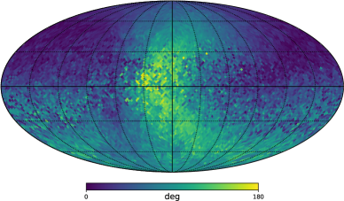
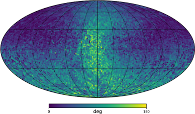
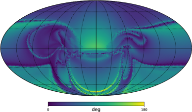
a) b)
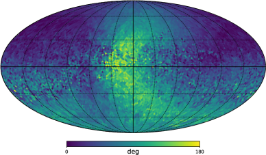
c) d)

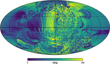
Figure 4: Absolute values of deflections of a 100 EeV iron nuclei from an initial arrival direction on its way to the Solar system in different models of the large-scale Galactic magnetic fields. Top panel: the JF12 model. Other panels: a) JF12P, b) JF12K, c) PTKN d) TF17. Galactic coordinates in the Mollweide projection are used.

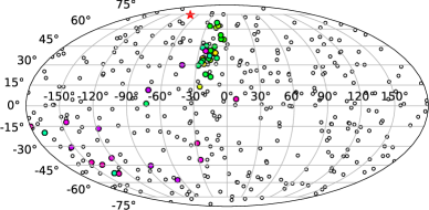
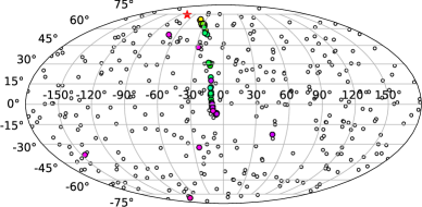
a) b)
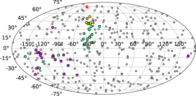
c) d)

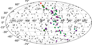
Figure 5: Examples of samples of 400 UHECRs with energies above 57 EeV with 14% of them coming from M 87 obtained with different models of the GMF: a) JF12P, b) JF12K, c) PTKN d) TF17. Compare them with the right panel in figure 3 showing the same for JF12.

To examine the robustness of the test statistic introduced in section 3, we have tested the original neural network classifier trained on the JF12 model on event sets generated assuming the four alternative GMF models described above. To make the test statistic more universal, we modified the early-stop procedure to avoid overfitting when training the classifier. Namely, we used a set of events prepared assuming the PTKN model of the GMF as validation data. Results of the tests are presented in table 2. Notice that similar to the results presented above, CNNs were trained separately for each particular source and the number of incoming UHECRs, with the background flux being isotropic.

Table 2: Results of tests of the CNNs trained with the JF12 model of the GMF versus data sets generated assuming other models. Here, JF12 is the original model [17, 18], JF12P is the JF12 model modified by the Planck Collaboration [28], JF12K is a version of the JF12 model suggested by Kleimann et al. [29], PTKN is a model by Pshirkov et al. [30] and TF17 is a model by Terral and Ferrière [31]. Numbers mean the same percentage as defined in table 1. A dash means a solution was not found. See figure 7 below for an illustration of the data for M 87.

Source	GMF	50	100	200	300	400	500
	JF12	14	10	6	5	3.75	3.6
	JF12P	20	13	8	6.7	5.5	5.2
NGC 253	JF12K	14	9	5.5	4.3	3.75	3.4
	PTKN	28	16	9.5	8	6.5	5.8
	TF17	64	42	24	18.3	14.25	12
	JF12	16	12	7.5	6	5.25	4.8
	JF12P	22	14	10	8	6.75	5.8
Cen A	JF12K	16	11	8	6.3	5.5	4.8
	PTKN	20	12	8	6	5.25	4
	TF17	40	25	19	13.7	12	10.4
	JF12	20	14	8.5	6.3	5.5	4.6
	JF12P	26	17	10	8	6.5	6.2
M 82	JF12K	24	15	9	7.3	6	5
	PTKN	20	12	7	5.3	4.25	3.8
	TF17	30	20	12.5	9.7	7.75	6.2
	JF12	24	17	11	8.3	7.5	6.6
	JF12P	46	22	17.5	11.67	10	8.6
M 87	JF12K	26	17	11.5	9	7.75	7
	PTKN	34	18	11	8.7	7	5.6
	TF17	–	79	44.5	33.7	26.5	24.2
	JF12	16	11	7.5	6	4.75	4.6
	JF12P	26	17	10.5	8.3	7	6.6
Fornax A	JF12K	16	10	6.5	5	4.5	3.8
	PTKN	26	16	10	7.7	5.5	5.4
	TF17	58	38	18	15	10.75	9.8

In general, the CNNs trained with the JF12 model demonstrate excellent robustness against the JF12K model, for which they sometimes produce even better results, possibly due to more compact patterns of arrival directions. The JF12P model is more complicated for the CNNs but results are still good for almost all sources except M 87, for which the minimum required fraction of from-source events grows strongly for small samples. The PTKN model acts sufficiently well sometimes demonstrating results that are even better than for the original JF12 model (see the case of M 82). Finally, the TF17 model presents the biggest problem for the CNNs trained for JF12. Still, except for M 87, even this model of the GMF works well enough to allow detecting a nearby source providing the size of the total sample is big enough. Thus, one can conclude that the suggested CNNs demonstrate good efficiency providing the main features of the Galactic magnetic field are understood sufficiently well. Notice the new CNNs perform slightly worse for the JF12 model than those used in table 1 due to the early-stop procedure, which is non-optimal for them. An important point is the CNNs can be easily updated as soon as our knowledge of the large-scale GMF improves.

4.2 Testing the CNNs against different mass compositions

4.2.1 Mass composition as a function of the propagation length in the KKOS model

It is known that mass composition of UHECRs registered on Earth depends on the distance to the source. One and the same AGN located at different distances from Earth will generate UHECRs with possibly distinguishable mass compositions due to interactions nuclei face on their way from the source. This results in different patterns of their arrival directions. Figure 6 illustrates how mass composition of UHECRs registered at Earth depends on the propagation length in the KKOS model.

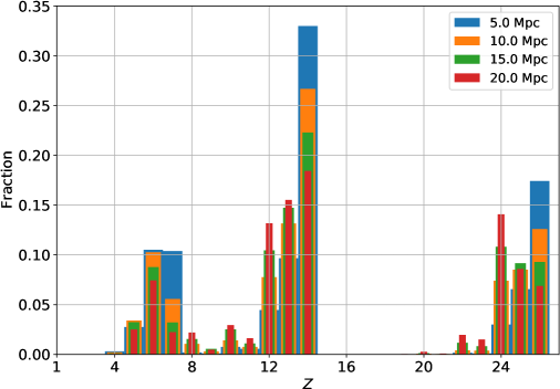
Figure 6: Dependence of the mass composition of UHECRs above 57 EeV on the distance to the source in the KKOS model. The height of bins is normalised to the total flux. $Z$ is the atomic number of a nuclei.

We used distances given in the catalogue [33] rounded to 0.5 Mpc for the sources considered above. On the other hand, the NASA/IPAC Extragalactic Database (NED) provides a whole range of distances to the objects. We took the mean values plus/minus standard deviations and tested the CNNs used to obtain table 1 against maps of arrival directions obtained for samples arriving from the minimum and maximum distances defined this way. It was found that percentage of from-source events necessary to verify the original null hypothesis $H_{0}$ deviates by at most 10% from the numbers given in table 1 even for Fornax A, which has the biggest uncertainty in the distance, thus demonstrating an excellent robustness of the CNNs in these tests.

4.2.2 Comparison with other mass compositions

Mass composition of UHECRs is a subject of ongoing studies and debates. It is known that results of the Telescope Array (TA) experiment witness in favour of a light mass composition in the whole energy range above a few EeV [34] while the Pierre Auger Observatory argues that the UHECR flux at around 2 EeV mostly consists of light nuclei but becomes heavier at higher energies [35]. The TA collaboration has recently suggested a mass composition that fits well the data of both experiments. It consists of protons (57%), nuclei of helium (18%), nitrogen (17%) and iron (8%) [34]. We will refer to this composition as TA4. We have considered how the CNNs presented in subsection 4.1 (trained with the KKOS mass composition and the JF12 model of the GMF model) perform with this new composition. Besides this, we tested the CNNs against two other mass compositions, one of which being in average two times lighter than the original composition in the KKOS model, and another one being two times heavier. Compositions in these two models are probably unnatural. We introduced them just to evaluate the robustness of the test statistics obtained in subsection 4.1. Results of the tests are presented in table 3.

Table 3: Results of tests of the CNNs used in subsection 4.1 versus different mass compositions of UHECRs. Here, “Mass” denoted as “0.5” corresponds to the mass composition that is in average two times lighter than that in the original KKOS model, “2.0” denotes a composition that is two times heavier. “TA4” denotes the 4-component composition suggested by the Telescope Array collaboration [34]. Numbers denote the same minimum percentage of UHECRs necessary to verify the null hypothesis $H_{0}$ as in all tables above. See figure 7 below for an illustration of the data for M 87.

Source	Mass	50	100	200	300	400	500
	0.5	12	8	5.5	4	3.5	3.4
NGC 253	2.0	18	13	9	6	5.25	4.8
	TA4	26	15	10	7.33	6.25	5.4
	0.5	14	9	6	4.67	4.25	3.6
Cen A	2.0	22	14	10	8	6.5	6
	TA4	14	8	4.5	3.3	2.75	2.2
	0.5	10	6	3.5	2.3	2	1.6
M 82	2.0	52	34	25	20	16.75	14.8
	TA4	8	5	3	2	1.75	1.4
	0.5	14	10	5.5	4.3	3.75	3
M 87	2.0	60	35	27	22	17.5	16
	TA4	24	14	8.5	6.67	5.5	4.6
	0.5	14	10	5	4.3	3.5	3
Fornax A	2.0	28	19	15	10.67	9.25	9
	TA4	18	14	7	5.3	4	3.6

As one could expect, the light composition (“0.5”) does not pose a problem for the CNNs since patterns of UHECR arrival directions become less fuzzy. More than this, the CNNs demonstrate even better results in this case than with the original composition, c.f. results corresponding to the JF12 model in table 2. The heavy (“2.0”) composition also worked fine for all sources except M 82 and M 87. This does not come as a surprise since light nuclei arriving from these two sources form long and narrow “tails” on the celestial sphere while heavy ones are spread over huge regions, see the right panel in figure 3 for M 87 and figure 4 in Paper 1 for M 82. As for the TA4 composition, results also depend on the particular source. The CNNs demonstrated good performance for Cen A, Fornax A and especially M 82 but needed higher percentage of events coming from M 87 and NGC 253 to verify $H_{0}$ for small samples. Generally, we conclude the CNNs exhibit good robustness to reasonable variations of the mass composition used for their training. Thus, the present uncertainty in the composition of UHECRs is not crucial for their application.

5 Multiple nearby sources of UHECRs

So far we considered the case of a single nearby source of UHECRs, and the problem was to reject the null hypothesis $H_{0}$ (isotropy) providing an alternative hypothesis (anisotropy) is true. To solve the task, we trained a separate classifier for each particular source and each size of the total sample to use it as a test statistic. A possibly more realistic situation is when there are two or more nearby sources contributing to the flux of UHECRs.

In Paper 1, we estimated the average event number coming from the second strongest source in case of identical sources to be roughly about 1/3 of the main source contribution (see Table 3 in Paper 1). Here, we have evaluated the performance of the test statistics obtained for Cen A being the only nearby source in a situation when there is another strong source, and test samples contain three times more events from Cen A than from that other source. The tests were performed for the JF12 model as well as for the other four models of the GMF. The results are presented in table 4. Notice that numbers given in the table denote percentage of the joint flux from Cen A and the second source relative to the total flux.

Table 4: Application of the test statistics based on classifiers trained on Cen A (rows 6-10 of table 2) to samples containing an admixture of events from another source. In test samples, the average number of events from the second source was three times less than from Cen A. Notation is the same as in table 2 except the percentage of the joint flux from Cen A and the second source relative to the total flux is shown now. See figure 7 below for an illustration of the data for M 87.

2nd source	GMF	50	100	200	300	400	500
	JF12	24	16	10.5	8	7	6.8
	JF12P	32	22	14	10.33	9.5	8.4
NGC 253	JF12K	24	18	11.5	8.67	7.25	6.8
	PTKN	30	18	12	8.33	7.25	6.2
	TF17	60	40	27	18.67	17.25	15
	JF12	26	17	11	8.33	6.75	6.4
	JF12P	32	22	14	11	9.25	7.8
M 82	JF12K	26	17	11	9	7.25	6.8
	PTKN	32	18	11	8.33	7.25	6.2
	TF17	62	40	26	19.67	17.75	13.6
	JF12	24	15	10.5	8	7	6.4
	JF12P	32	20	13.5	10.33	9.5	7.8
M 87	JF12K	24	15	10	8.33	7	6.4
	PTKN	28	17	11.5	9	7.25	5.8
	TF17	60	38	28	19	16.25	13.8
	JF12	26	16	10	8.67	7.25	6.4
	JF12P	34	21	15	11	9.5	8.2
Fornax A	JF12K	26	17	11	8.67	7.5	7.2
	PTKN	32	19	12	9	7.75	6.2
	TF17	62	38	29	19	18	15.4

An important point to notice about results presented in table 4 is that efficiency of the classifier remains high when tested on the JF12 model with the total fraction of UHECRs coming from any of the four pairs of sources being in the range 15–17% for $N=100$ and 6.4–6.8% for $N=500$. Nearly the same fractions are needed if the CNNs are tested on the JF12K model. As expected, other models of the GMF need a higher contribution of from-source events but there is no drastic decrease of performance in comparison with the case of a single source, cf. table 2.

Now, let us discuss what can be done in a more general case. It is straightforward to train a CNN for a set of nearby sources, e.g., Cen A, Fornax A and M 87, which are often considered as the most likely candidates. However, one needs to estimate relative fluxes of UHECRs arriving from the selected sources in the given energy range.

To the best of our knowledge, there is no unequivocal solution to the problem yet. It is argued by a number of authors that in the case of radio AGN, the UHECR flux generated by a particular source is proportional to its radio luminosity, see, e.g, [36, 37]. One can scale fluxes from each AGN taking them proportional to their radio luminosity at some frequency (say, at 1.4 GHz as was done in the catalogue [33]) divided by the square of the distance to the source. Applying this approach, one immediately finds that Cen A, which is a strong and nearby radio AGN, dominates the flux from the sources considered above, with only approximately 17% of it attributed to M 87 and Fornax A. This results in a situation very similar to the case of Cen A being the only source of a large-scale anisotropy with just a slightly higher fraction of from-source events necessary to observe a deviation from isotropy. Another approach relates the flux of UHECRs to the gamma-ray luminosity of sources [38] (see [39] for a recent application of the approach). In this case, Cen A also dominates the UHECR flux but in a different proportion to the flux of other sources.

To avoid the necessity of estimating the relative flux of possible nearby sources, we tried a more generic way. Namely, we assumed that any of the three sources — Cen A, M 87 and Fornax A — can be a dominating one but we do not know which of them. Then we trained classifiers with samples created the same way as in the cases discussed above, i.e., with a contribution from one of them and an isotropic background, but the source was chosen from the three in a random fashion for each new training sample. Once again, the CNNs were trained with the JF12 model of the GMF with the PTKN model employed for creating validation sets in the early-stop procedure.

After training the CNNs, we tested them against the same null hypothesis $H_{0}$ of isotropy as above. Notice that training was performed with three sources but tests were run for each of them separately. We also tested the performance of the CNNs for two “unknown” sources — NGC 253 and M 82, which were not anyhow involved in training. Finally, we checked how robust are the new classifiers against other models of the GMF. Results demonstrating the test statistic performance are presented in table 5.

Table 5: Results of tests of the CNNs trained simultaneously for three sources (Cen A, M 87 and Fornax A) assuming only one of them is contributing to a large-scale anisotropy of the flux. NGC 253 and M 82 were not involved in training. Notation is the same as in table 2. See figure 7 below for an illustration of the data for M 87.

Source	GMF	50	100	200	300	400	500
	JF12	22	14	9.5	7.3	6.25	5.6
	JF12P	24	16	11	8.3	7	5.6
Cen A	JF12K	24	15	9.5	7.67	6.5	5.8
	PTKN	22	14	9	7	5.25	4.4
	TF17	42	27	18.5	15	11	9.4
	JF12	28	19	12	11	9.5	7.8
	JF12P	58	36	26.5	22	19.5	11.8
M 87	JF12K	30	20	13	11.3	9	8
	PTKN	32	20	12	9.67	8.75	6
	TF17	–	95	60.5	39.7	31.23	26.4
	JF12	18	13	8	6.3	6	5.2
	JF12P	32	19	13	10.3	9	8
Fornax A	JF12K	18	12	7.5	6	5	5
	PTKN	36	21	14	10	8.5	8.4
	TF17	70	41	24	17	15.5	15.2
	JF12	36	22	15.5	11.67	10.25	8.2
	JF12P	76	48	31.5	25	22	15.8
NGC 253	JF12K	32	20	12.5	9.7	8.25	6.4
	PTKN	–	88	63.5	48	41.5	26.8
	TF17	–	75	61.5	42.3	34	29.8
	JF12	50	32	20	15	13.25	10.4
	JF12P	50	32	18.5	15.3	12.75	10.2
M 82	JF12K	50	32	20	15.3	12.25	10.8
	PTKN	32	22	13	10.3	9	7.4
	TF17	48	28	18	13.7	12	10

One can see the efficiency of the classifiers did not decrease drastically for the three sources used for training in comparison with the “ideal” case shown in table 2, except for M 87 and the TF17 model. The CNNs performed pretty well in all cases providing the test model of the GMF does not deviate strongly from the one used for training. The situation with the “unknown” sources is more complicated and varies depending on the source and the GMF model. The neural networks performed pretty well for NGC 253 with the JF12 and JF12K models, especially for $N\geq 200$, but not the other models of the GMF. Surprisingly, the best results for M 82 were obtained with the PTKN model, which outperformed all models of the JF family.

Finally, figure 7 illustrates the data presented in tables 2–5 for M 87.

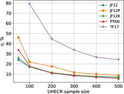
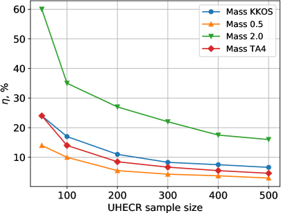
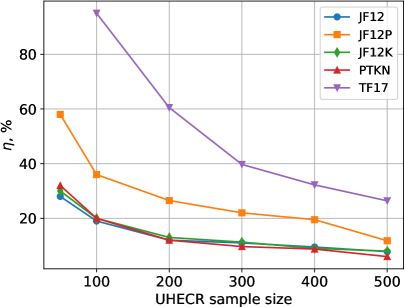
Figure 7: Illustration of the data presented in tables 2 (top left), 3 (top right), 4 (bottom left) and 5 (bottom right) for M 87.

6 Conclusions

We have demonstrated how one can strongly improve the efficiency of an analysis of arrival directions of UHECRs using machine learning techniques. The basic idea is to train a classifier which discriminates samples generated assuming null (isotropy) and alternative (anisotropy) hypotheses and to use the classifier output as a test statistic. An application of models that involve pattern recognition such as the suggested deep convolutional neural network on a HEALPix grid gives a really qualitative enhancement in terms of sensitivity to deviations from an isotropic distribution of arrival directions. It was shown in particular that the method allows decreasing the minimal number of events necessary to reject the null hypothesis by $\sim 4$ times. This reduces technical demands and the required total exposure of an UHECR experiment drastically.

Although the new test statistic depends on the alternative model details such as the choice of a nearby source, the Galactic magnetic field configuration, the spectrum and mass composition of cosmic rays, we proposed a couple of methods to make it less model dependent. The first idea is to use sample sets derived in a modified model as validation data for the early-stop technique to avoid overfitting. The second idea is to use several sources for building the classifier training samples to obtain a more universal test statistic.

Note that the test statistic model dependence is not necessarily a drawback for the source identification problem. We intentionally started our discussion from the test statistics trained with a particular source in mind since these statistics are the most sensitive to the flux from that source and can be used to reject the hypothesis of the particular source giving the main contribution to the anisotropy. As an illustration, we tried to reject the null hypothesis of Cen A giving at least 6% of events, assuming that we have observed 300 events and a large-scale anisotropy has been established as above. We needed to formulate an alternative hypothesis to do this. We just repeated our previous calculations with null and alternative hypothesis swapped in the case of isotropy being an alternative hypothesis. This way, we obtained $\beta\leq 0.048$ for $\alpha=0.01$ using the test statistic based on the previously trained CNN classifier, discriminating maps with an admixture of Cen A events from isotropic maps. A less trivial question is whether one can use the same test statistic with another alternative hypothesis, e.g., assuming another source giving the main contribution to the anisotropy. To answer this question, we calculated the same Cen A-based test statistic on maps with an admixture of 6% events from one of the other four sources, considered in the work. We obtained values of $\beta$ in the range from 0.02 for M 82 to 0.16 for Fornax A, assuming $\alpha=0.01$ as above, thus indicating the usefulness of the test statistic derived. However, a more efficient test statistic can be constructed for any specific alternative hypothesis by training the CNN classifier on the corresponding null and alternative hypotheses maps.

We emphasise the proposed method can be applied in more complicated situations than those discussed above. For instance, we considered the case of a uniform exposure of the celestial sphere, which is expected for orbital detectors like K-EUSO or POEMMA but a non-uniform exposure, which takes place for the existing ground-based experiments, is not a problem here since it can be easily taken into account when generating training and validation sets of data. Besides this, one can employ other possible sources of UHECRs and their combinations to study more cases. Last but not least, the presented CNN is modest on computational resources allowing one to perform the whole analysis on an average desktop computer not necessarily equipped with a GPU.

Finally, we remark that training one CNN for each particular source and each size $N$ of UHECR samples was a big work. A reasonable question is whether one can reduce the amount of calculations. The answer is yes. Namely, we have tested two CNNs for each of the sources (for the JF12 model), one trained for samples of the size $N=50$ and another one for $N=500$, against the whole range of sample sizes. A remarkable thing is the difference between results obtained with “dedicated” CNNs as shown in tables 1 or 2 and those obtained for CNNs trained for $N=50$ or 500 was negligible.

In the future, we plan to take into account uncertainties in the energy of detected UHECRs, which influence the spectrum and thus the shape of patterns formed by nuclei arriving from a source. It is also interesting to check if a further improvement in recognizing patterns of arrival directions and thus identifying sources of UHECRs can be obtained by changing the energy threshold of events selected for the analysis and by incorporating information on the energy or the depth of maximum of registered events in a neural network. We believe the suggested approach opens new promising possibilities for studying anisotropy of ultra-high-energy cosmic rays and identifying their sources. The source code and supplemental materials for this work, including trained classifier models, can be downloaded from the project web page [23].

References

- [1] J. Linsley, L. Scarsi and B. Rossi, Extremely energetic cosmic-ray event, Physical Review Letters 6 (1961) 485.
- [2] M. Casolino, P. Klimov and L. Piotrowski, Observation of ultra high energy cosmic rays from space: Status and perspectives, Progress of Theoretical and Experimental Physics 2017 (2017) .
- [3] P. Klimov, M. Casolino and the JEM-EUSO Collaboration, Status of the KLYPVE-EUSO detector for EECR study on board the ISS, in Proceedings, 35th International Cosmic Ray Conference (ICRC 2017): Bexco, Busan, Korea, July 12-20, 2017, p. 412, 2017, https://pos.sissa.it/301/412/pdf.
- [4] M. Casolino, A. Belov, M. Bertaina, T. Ebisuzaki and the JEM-EUSO Collaboration, KLYPVE-EUSO: science and UHECR observational capabilities, in Proceedings, 35th International Cosmic Ray Conference (ICRC 2017): Bexco, Busan, Korea, July 12-20, 2017, p. 368, 2017, https://pos.sissa.it/301/368/pdf.
- [5] G. K. Garipov, M. Y. Zotov, P. A. Klimov, M. I. Panasyuk, O. A. Saprykin, L. G. Tkachev et al., The KLYPVE ultra high energy cosmic ray detector on board the ISS, Bull. Rus. Acad. Sci. Physics 79 (2015) 326.
- [6] A. V. Olinto, J. Adams, R. Aloisio, L. Anchordoqui, D. Bergman and M. Bertaina, POEMMA: Probe Of Extreme Multi-Messenger Astrophysics, in 36th International Cosmic Ray Conference (ICRC2019), vol. 36 of International Cosmic Ray Conference, p. 378, Jul, 2019, 1907.06217.
- [7] A. V. Olinto, J. H. Adams, R. Aloisio, L. A. Anchordoqui, D. R. Bergman, M. E. Bertaina et al., POEMMA: Probe Of Extreme Multi-Messenger Astrophysics, in Proceedings, 35th International Cosmic Ray Conference (ICRC 2017): Bexco, Busan, Korea, July 12-20, 2017, vol. 301, p. 542, 2017, 1708.07599.
- [8] O. Kalashev, M. Pshirkov and M. Zotov, Prospects of detecting a large-scale anisotropy of ultra-high-energy cosmic rays from a nearby source with the K-EUSO orbital telescope, Journal of Cosmology and Astroparticle Physics 2019 (2019) 034.
- [9] M. Kachelrieß, O. Kalashev, S. Ostapchenko and D. V. Semikoz, Minimal model for extragalactic cosmic rays and neutrinos, Phys. Rev. D96 (2017) 083006 [1704.06893].
- [10] G. Carleo, I. Cirac, K. Cranmer, L. Daudet, M. Schuld, N. Tishby et al., Machine learning and the physical sciences, Reviews of Modern Physics 91 (2019) 045002 [1903.10563].
- [11] K. M. Górski, E. Hivon, A. J. Banday, B. D. Wandelt, F. K. Hansen, M. Reinecke et al., HEALPix: A framework for high-resolution discretization and fast analysis of data distributed on the sphere, Astrophys. J. 622 (2005) 759 [astro-ph/0409513].
- [12] J. Hülss and C. Wiebusch, Search for signatures of extra-terrestrial neutrinos with a multipole analysis of the AMANDA-II sky-map, in Proceedings, 30th International Cosmic Ray Conference (ICRC 2007): Merida, Mexico, July 3–11 2007, 2007, 0711.0353.
- [13] Pierre Auger collaboration, Multi-resolution anisotropy studies of ultrahigh-energy cosmic rays detected at the Pierre Auger Observatory, Journal of Cosmology and Astroparticle Physics 1706 (2017) 026 [1611.06812].
- [14] O. E. Kalashev and E. Kido, Simulations of ultra high energy cosmic rays propagation, J. Exp. Theor. Phys. 120 (2015) 790 [1406.0735].
- [15] M. S. Pshirkov, P. G. Tinyakov and F. R. Urban, New limits on extragalactic magnetic fields from rotation measures, Phys. Rev. Lett. 116 (2016) 191302 [1504.06546].
- [16] R. Alves Batista, A. Dundovic, M. Erdmann, K.-H. Kampert, D. Kuempel, G. Müller et al., CRPropa 3—a public astrophysical simulation framework for propagating extraterrestrial ultra-high energy particles, Journal of Cosmology and Astroparticle Physics 1605 (2016) 038 [1603.07142].
- [17] R. Jansson and G. R. Farrar, A new model of the Galactic magnetic field, Astrophys. J. 757 (2012) 14 [1204.3662].
- [18] R. Jansson and G. R. Farrar, The Galactic magnetic field, Astrophysical Journal Letters 761 (2012) L11 [1210.7820].
- [19] Y. LeCun, B. Boser, J. S. Denker, D. Henderson, R. E. Howard, W. Hubbard et al., Backpropagation applied to handwritten zip code recognition, Neural Computation 1 (1989) 541.
- [20] T. S. Cohen, M. Geiger, J. Koehler and M. Welling, Spherical CNNs, in International Conference on Learning Representations, p. 542, 2018, 1801.10130.
- [21] N. Perraudin, M. Defferrard, T. Kacprzak and R. Sgier, DeepSphere: Efficient spherical convolutional neural network with HEALPix sampling for cosmological applications, Astron. Comput. 27 (2019) 130 [1810.12186].
- [22] N. Krachmalnicoff and M. Tomasi, Convolutional neural networks on the HEALPix sphere: a pixel-based algorithm and its application to CMB data analysis, Astron. Astrophys. 628 (2019) A129 [1902.04083].
- [23] O. Kalashev, M. Pshirkov and M. Zotov, “Supplemental materials and source code for this work.” https://github.com/okolo/ml_cr_aniso, 2020.
- [24] F. Chollet et al., “Keras.” https://keras.io, 2015.
- [25] M. D. Zeiler, ADADELTA: an adaptive learning rate method, CoRR (2012) [1212.5701].
- [26] R. U. Abbasi, M. Abe, T. Abu-Zayyad, M. Allen, R. Anderson, R. Azuma et al., Indications of intermediate-scale anisotropy of cosmic rays with energy greater than 57 EeV in the Northern sky measured with the surface detector of the Telescope Array experiment, Astrophysical Journal Letters 790 (2014) L21 [1404.5890].
- [27] Pierre Auger Collaboration, A. Aab, P. Abreu, M. Aglietta, I. A. Samarai, I. F. M. Albuquerque et al., Observation of a large-scale anisotropy in the arrival directions of cosmic rays above eV, Science 357 (2017) 1266 [1709.07321].
- [28] Planck Collaboration, R. Adam, P. A. R. Ade, M. I. R. Alves et al., Planck intermediate results. XLII. Large-scale Galactic magnetic fields, Astronomy & Astrophysics 596 (2016) A103 [1601.00546].
- [29] J. Kleimann, T. Schorlepp, L. Merten and J. B. Tjus, Solenoidal improvements for the JF12 Galactic magnetic field model, The Astrophysical Journal 877 (2019) 76 [1809.07528].
- [30] M. S. Pshirkov, P. G. Tinyakov, P. P. Kronberg and K. J. Newton-McGee, Deriving global structure of the Galactic magnetic field from Faraday rotation measures of extragalactic sources, Astrophys. J. 738 (2011) 192 [1103.0814].
- [31] P. Terral and K. Ferrière, Constraints from Faraday rotation on the magnetic field structure in the Galactic halo, Astronomy & Astrophysics 600 (2017) A29 [1611.10222].
- [32] K. Ferrière and P. Terral, Analytical models of X-shape magnetic fields in galactic halos, Astronomy & Astrophysics 561 (2014) A100 [1312.1974].
- [33] S. van Velzen, H. Falcke, P. Schellart, N. Nierstenhöfer and K.-H. Kampert, Radio galaxies of the local universe. All-sky catalog, luminosity functions, and clustering, Astronomy & Astrophysics 544 (2012) A18 [1206.0031].
- [34] W. Hanlon, Telescope Array 10 year composition, in 36th International Cosmic Ray Conference (ICRC2019), vol. 36 of International Cosmic Ray Conference, p. 280, July, 2019, 1908.01356.
- [35] A. Yushkov, Mass composition of cosmic rays with energies above eV from the hybrid data of the Pierre Auger Observatory, in 36th International Cosmic Ray Conference (ICRC2019), vol. 36 of International Cosmic Ray Conference, p. 482, July, 2019.
- [36] I. Duţan and L. I. Caramete, Ultra-high-energy cosmic rays from low-luminosity active galactic nuclei, Astroparticle Physics 62 (2015) 206 [1409.8162].
- [37] J. P. Rachen and B. Eichmann, A parametrized catalog of radio galaxies as UHECR sources, in 36th International Cosmic Ray Conference (ICRC2019), vol. 36 of International Cosmic Ray Conference, p. 396, July, 2019, 1909.00261.
- [38] C. D. Dermer and S. Razzaque, Acceleration of ultra-high-energy cosmic rays in the colliding shells of blazars and gamma-ray bursts: Constraints from the Fermi Gamma-ray Space Telescope, Astrophysical Journal 724 (2010) 1366 [1004.4249].
- [39] A. Aab, P. Abreu, M. Aglietta et al., An indication of anisotropy in arrival directions of ultra-high-energy cosmic rays through comparison to the flux pattern of extragalactic gamma-ray sources, Astrophysical Journal Letters 853 (2018) L29 [1801.06160].
- [40] M. Wenger, F. Ochsenbein, D. Egret, P. Dubois, F. Bonnarel, S. Borde et al., The SIMBAD astronomical database. The CDS reference database for astronomical objects, Astronomy and Astrophysics Supplement 143 (2000) 9 [astro-ph/0002110].