Time-variation in online nonconvex optimization enables escaping from spurious local minima
Abstract
A major limitation of online algorithms that track the optimizers of time-varying nonconvex optimization problems is that they focus on a specific local minimum trajectory, which may lead to poor spurious local solutions. In this paper, we show that the natural temporal variation may help simple online tracking methods find and track time-varying global minima. To this end, we investigate the properties of a time-varying projected gradient flow system with inertia, which can be regarded as the continuous-time limit of (1) the optimality conditions for a discretized sequential optimization problem with a proximal regularization and (2) the online tracking scheme. We introduce the notion of the dominant trajectory and show that the inherent temporal variation could re-shape the landscape of the Lagrange functional and help a proximal algorithm escape the spurious local minimum trajectories if the global minimum trajectory is dominant. For a problem with twice continuously differentiable objective function and constraints, sufficient conditions are derived to guarantee that no matter how a local search method is initialized, it will track a time-varying global solution after some time. The results are illustrated on a benchmark example with many local minima.
Index Terms:
Time-varying optimization, nonconvex optimization, stability analysis.I Introduction
In this paper, we study the following equality-constrained time-varying optimization problem:
| (1) | ||||
| s.t. |
where denotes the time and is the optimization variable that depends on . Moreover, the objective function and the constraint function with for are assumed to be twice continuously differentiable in state and continuously differentiable in time . For each time , the function could potentially be nonconvex in with many local minima and the function could also potentially be nonlinear in , leading to a nonconvex feasible set. The objective is to solve the above problem online under the assumption that at any given time the function and are known for all while no knowledge about or may be available for any . Therefore, the problem (1) cannot be minimized off-line and should be solved sequentially. Another issue is that the optimization problem at each time instance could be highly complex due to NP-hardness, which is an impediment to finding its global minima. This paper aims to investigate under what conditions simple local search algorithms can solve the above online optimization problem to almost global optimality after some finite time. More precisely, the goal is to devise an algorithm that can track a global solution of (1) as a function of time with some error at the initial time and a diminishing error after some time.
If and do not change over time, the problem reduces to a classic (time-invariant) optimization problem. It is known that simple local search methods, such as stochastic gradient descent (SGD) [2], may be able to find a global minimum of such time-invariant problems (under certain conditions) for almost all initializations due to the randomness embedded in SGD [3, 4, 5]. The objective of this paper is to significantly extend the above result from a single optimization problem to infinitely-many problems parametrized by time . In other words, it is desirable to investigate the following question: Can the temporal variation in the landscape of time-varying nonconvex optimization problems enable online local search methods to find and track global trajectories? To answer this question, we study a first-order time-varying ordinary differential equation (ODE), which is the counterpart of the classic projected gradient flow system for time-invariant optimization problems [6] and serves as a continuous-time limit of the discrete online tracking method for (1) with the proximal regularization. This ODE is given as
| (P-ODE) |
where is a constant parameter named inertia due to a proximal regularization, , and are matrices related to the Jacobian of that will be derived in detail later. A system of the form (P-ODE) is called a time-varying projected gradient system with inertia . The behavior of the solutions of this system initialized at different points depends on the value of . In the unconstrained case, this ODE reduces to the time-varying gradient system with inertia given as
| (ODE) |
In what follows, we offer a motivating example without constraints (to simplify the visualization) before stating the goals of this paper.
I-A Motivating example
Example 1.
Consider , where
This time-varying objective has a spurious (non-global) local minimum trajectory at , a local maximum trajectory at , and a global minimum trajectory at . In Figure 1, we show a bifurcation phenomenon numerically. The red lines are the solutions of (P-ODE) with the initial point . In the case with and , the solution of (P-ODE) winds up in the region of attraction of the global minimum trajectory. However, for the case with and , the solution of (P-ODE) remains in the region of attraction of the spurious local minimum trajectory. In the case with and , the solution of (P-ODE) fails to track any local minimum trajectory. In the case with and , the solution of (P-ODE) winds up in the region of attraction of the global minimum trajectory.
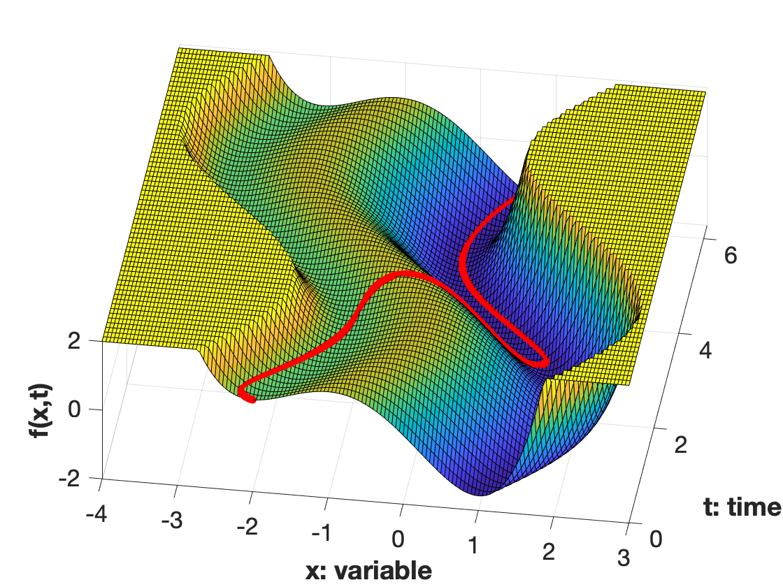
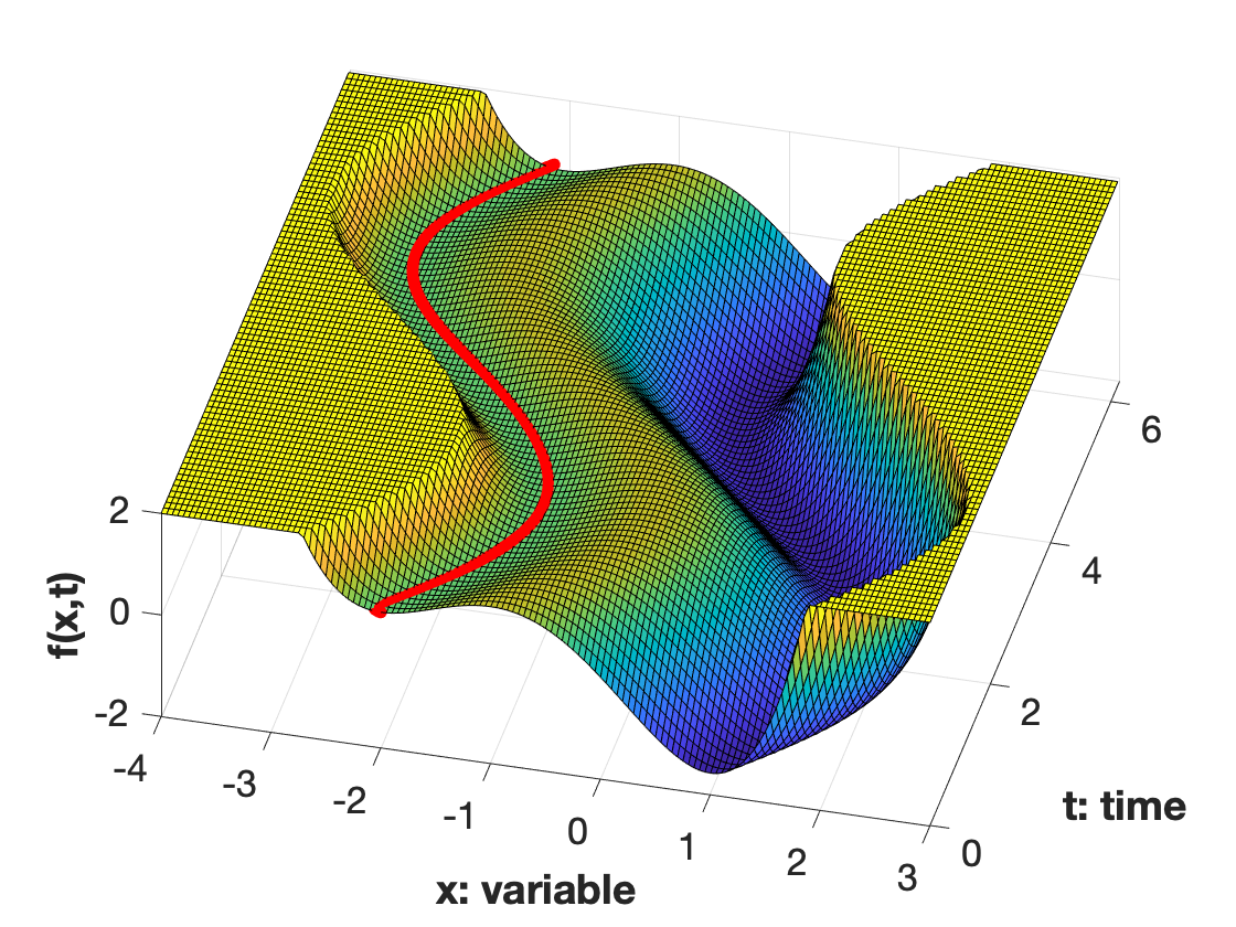
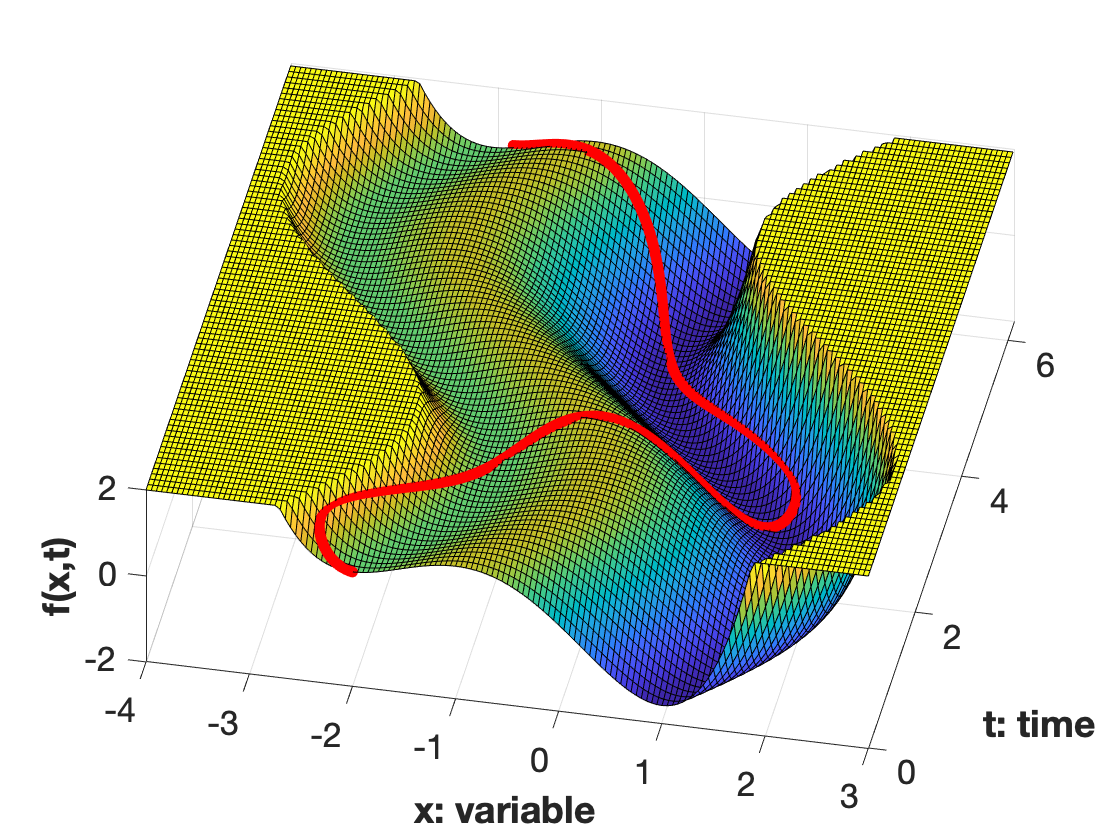
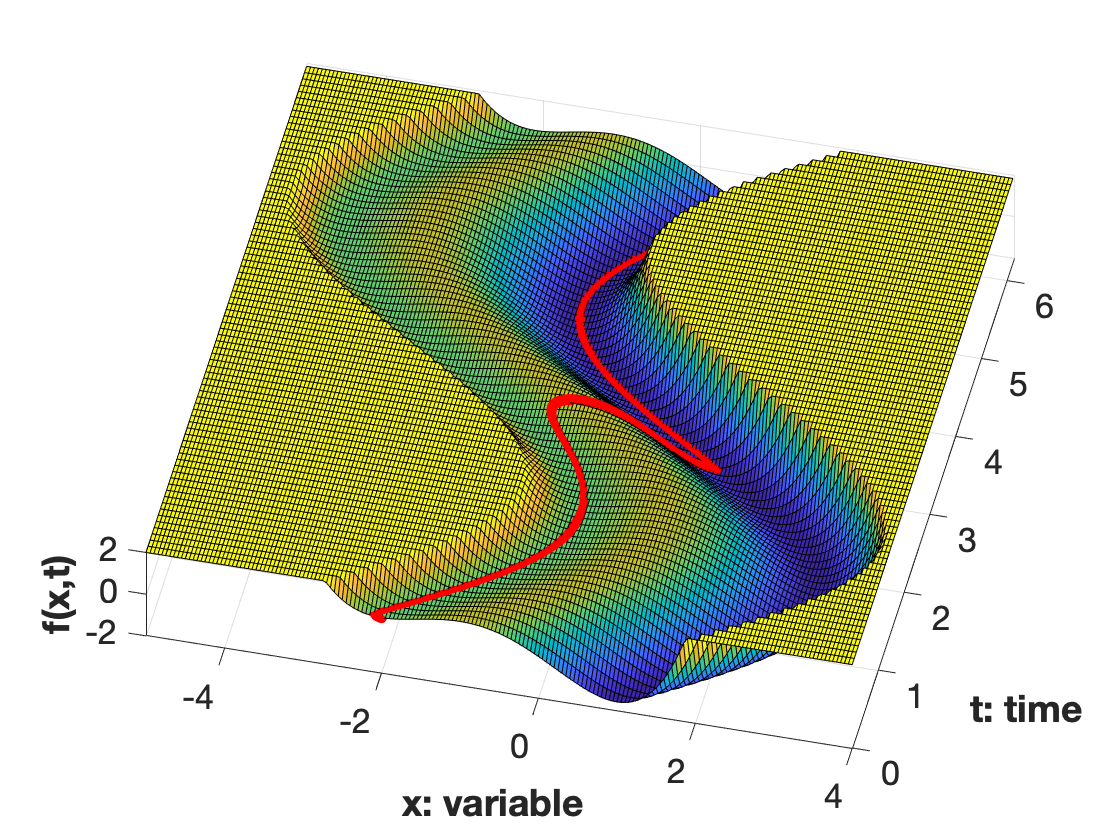
Two observations can be made here. First, jumping from a local minimum trajectory to a better trajectory tends to occur with the help of a relatively large inertia when the local minimum trajectory changes the direction abruptly and there happens to exist a better local minimum trajectory in the direction of the inertia. Second, when the inertia is relatively small, the solution of (P-ODE) tends to track a local (or global) minimum trajectory closely and converges to that trajectory quickly.
Example 2.
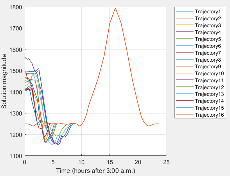
Consider the time-varying optimal power flow (OPF) problem, as the most fundamental problem for the operation of electric power grids that aims to match supply with demand while satisfying network and physical constraints. Let be the function to be minimized at time , which is the sum of the total energy cost and a penalty term taking care of all the inequality constraints of the problem. Let describe the time-varying demand constraint. Assume that the load data corresponds to the California data for August 2019. As discussed in [7], this time-varying OPF has 16 local minima at t=0 and many more for some values of . However, if (ODE) is run from any of these local minima, the 16 trajectories will all converge to the globally optimal trajectory, as shown in Figure 2. This observation has been made in [7] for a discrete-time version of the problem, but it also holds true for the continuous-time (ODE) model.
I-B Our contributions
To mathematically study the observations made in Example 1 and Example 2 for a general time-varying nonconvex optimization problem with equality constraints, we focus on the aforementioned time-varying projected gradient flow system with inertia as a continuous-time limit of an online updating scheme for (1). We first introduce a time-varying Lagrange functional to unify the analysis of unconstrained problems and equality-constrained problems, and make the key assumption that the time-varying Lagrange functional is locally one-point strongly convex around each local minimum trajectory. This assumption is justified by the second-order sufficient optimality conditions. A key property of (P-ODE) is that its solution will remain in the time-varying feasible region if the initial point is feasible for (1), which allows us to use the Lyapunov technique without worrying about the feasibility of the solution. Then, we show that the time-varying projected gradient flow system with inertia is a continuous-time limit of the Karush–Kuhn–Tucker (KKT) optimality conditions for a discretized sequential optimization problem with a proximal regularization. The existence and uniqueness of the solution for such ODE is proven.
As a main result of this work, it is proven that the natural temporal variation of the time-varying optimization problem encourages the exploration of the state space and re-shaping the landscape of the objective function (in the unconstrained case) or the Langrange functional (in the constrained case) by making it one-point strongly convex over a large region during some time interval. We introduce the notion of the dominant trajectory and show that if a given spurious local minimum trajectory is dominated by the global minimum trajectory, then the temporal variation of the time-varying optimization would trigger escaping the spurious local minimum trajectory for free. We develop two sufficient conditions under which the ODE solution will jump from a certain local minimum trajectory to a more desirable local minimum trajectory. We then derive sufficient conditions on the inertia to guarantee that the solution of (P-ODE) can track a global minimum trajectory. To illustrate how the time variation nature of an online optimization problem promotes escaping a spurious minimum trajectory, we offer a case study with many shallow minimum trajectories.
I-C Related work
Online time-varying optimization problems: Time-varying optimization problems of the form (1) arise in the real-time optimal power flow problem [8, 9] for which the power loads and renewable generations are time-varying and operational decisions should be made every 5 minutes, as well as in the real-time estimation of the state of a nonlinear dynamic system [10]. Other examples include model predictive control [11], time-varying compressive sensing [12, 13] and online economic optimization [14, 15]. There are many researches on the design of efficient online algorithms for tracking the optimizers of time-varying convex optimization problems [16, 17, 18, 19]. With respect to time-varying nonconvex optimization problems, the work [20] presents a comprehensive theory on the structure and singularity of the KKT trajectories for time-varying optimization problems. On the algorithm side, [8] provides regret-type results in the case where the constraints are lifted to the objective function via penalty functions. [21] develops a running regularized primal-dual gradient algorithm to track a KKT trajectory, and offers asymptotic bounds on the tracking error. [22] obtains an ODE to approximate the KKT trajectory and derives an algorithm based on a predictor-corrector method to track the ODE solution.
Recently, [23] proposed the question of whether the natural temporal variation in a time-varying nonconvex optimization problem could help a local tracking method escape spurious local minimum trajectories. It developed a differential equation to characterize this phenomenon (which is the basis of the current work), but it lacked mathematical conditions to guarantee this desirable behavior. The paper [7] also studies this phenomenon in the context of power systems and verifies on real data for California that the natural load variation enables escaping local minima of the optimal power flow problem. The current work significantly generalizes the results of [23] and [7] by mathematically studying when such an escaping is possible.
Local search methods for global optimization: Nonconvexity is inherent in many real-world problems: the classical compressive sensing and matrix completion/sensing [24, 25, 26], training of deep neural networks [27], the optimal power flow problem [28], and others. From the classical complexity theory, this nonconvexity is perceived to be the main contributor to the intractability of these problems. However, it has been recently shown that simple local search methods, such as gradient-based algorithms, have a superb performance in solving nonconvex optimization problems. For example, [29] shows that the gradient descent with a random initialization could avoid the saddle points almost surely, and [3] and [4] prove that a perturbed gradient descent and SGD could escape the saddle points efficiently. Furthermore, it has been shown that nearly-isotropic classes of problems in matrix completion/sensing [30, 31, 32], robust principle component analysis [33, 34], and dictionary recovery [35] have benign landscape, implying that they are free of spurious local minima. The work [5] proves that SGD could help escape sharp local minima of a loss function by taking the alternative view that SGD works on a convolved (thus smoothed) version of the loss function. However, these results are all for time-invariant optimization problems for which the landscape is time-invariant. In contrast, many real-world problems should be solved sequentially over time with time-varying data. Therefore, it is essential to study the effect of the temporal variation on the landscape of time-varying nonconvex optimization problems.
Continuous-time interpretation of discrete numerical algorithms: Many iterative numerical optimization algorithms for time-invariant optimization problems can be interpreted as a discretization of a continuous-time process. Then, several new insights have been obtained due to the known results for continuous-time dynamical systems [36, 37]. Perhaps, the simplest and oldest example is the gradient flow system for the gradient descent algorithm with an infinitesimally small step size. The recent papers [38, 39, 40] study accelerated gradient methods for convex optimization problems from a continuous-time perspective. In addition, the continuous-time limit of the gradient descent is also employed to analyze various non-convex optimization problems, such as deep linear neural networks [41] and matrix regression [42]. It is natural to analyze the continuous-time limit of an online algorithm for tracking a KKT trajectory of time-varying optimization problem [16, 21, 22, 23].
I-D Paper organization
This paper is organized as follows. Section II presents some preliminaries for time-varying optimization with equality constraints and the derivation of time-varying projected gradient flow with inertia. Section III offers an alternative view on the landscape of time-varying nonconvex optimization problems after a change of variables and explains the role of the time variation of the constraints. Section IV analyzes the jumping, tracking and escaping behaviors of local minimum trajectories. Section V illustrates the phenomenon that the time variation of an online optimization problem can assist with escaping spurious local minimum trajectories, by working on a benchmark example with many shallow minimum trajectories. Concluding remarks are given in Section VI.
I-E Notation
The notation represents the Euclidean norm. The interior of the interval is denoted by . The symbol denotes the region centered around a trajectory with radius at time . We denote the solution of starting from at the initial time with or the short-hand notation if the initial condition is clear from the context.
II Preliminaries and Problem Formulation
II-A Time-varying optimization with equality constraints
The first-order KKT conditions for the time-varying optimization (1) are as follows:
| (2a) | ||||
| (2b) | ||||
where denotes the Jacobian of with respect to the first argument and is a Lagrange multiplier associated with the equality constraint. We first make some assumptions below.
Assumption 1.
is twice continuously differentiable in and continuously differentiable in . is twice continuously differentiable in and twice continuously differentiable in for . Moreover, at any given time , is uniformly bounded from below over the set , meaning that there exists a constant such that for all and .
Assumption 2.
The feasible set at defined as
is nonempty for all .
Assumption 3.
For all and , the matrix has full row-rank.
Remark 1.
Although Assumption 3 is somewhat stronger than the Linear independence constraint qualification [43], it is necessary for our following analysis because with different values of and different initial points, the solution of (P-ODE) may land anywhere in the feasible region. Furthermore, Sard’s theorem [44] ensures that if the constraint function is sufficiently smooth, then the set of values of , denoted as (t), for which is not full row-rank has measure 0. Thus, Assumption 3 is satisfied if where is only a set with measure 0. Finally, if the inertia parameter is fixed and the initial point of (P-ODE) is a local solution, then the work [23] provides a sophisticated proof for the existence and uniqueness of the solution for a special class of (P-ODE) under a minor assumption that the Jacobian has full-row rank only at the discrete local trajectories (which is defined in the paragraph after equation (10) in our work). However, to be able to study the solution of (P-ODE) for all and any initial feasible point and keep the focus of the paper on studying the escaping behavior, we made Assumption 3.
Under Assumption 3, the matrix is invertible and therefore in (2a) can be written as
| (3) |
Since is written as a function of in (3), we also denote it as . Now, (2a) can be written as
| (4) |
where is the identity matrix in . For the sake of readability, we introduce the symbolic notation
which is the orthogonal projection operation onto , where denotes the tangent plane of at the point and the time . It is convenient and conventional to introduce the time-varying Lagrange functional
| (5) |
In terms of this functional, (II-A) can be written as
| (6) |
where is given in (3). Here, means first taking the partial gradient with respect to the first argument and then using the formula (3) for . Since the solution is time-varying, we define the notion of the local (or global) minimum trajectory below.
Definition 1.
In this paper, we focus on the case when the local minimum trajectories will not cross, bifurcate or disappear by assuming the following uniform regularity condition.
Assumption 4.
For each local minimum trajectory , its domain is and satisfies the second-order sufficient optimality conditions uniformly, meaning that is positive definite on for all .
Lemma 1.
Proof.
Under Assumptions 1-4, one can apply the inverse function theorem to (2) (see [45, Theorem 4.4, Example 4.7]) to conclude that for every and , there exist an open set containing and an open set containing such that there exist a unique differentiable function in for all where is the isolated local minimizer of the time-varying optimization problem (1). Because of this uniqueness property and the continuity of the local minimum trajectory , must coincide with for all . Then, because the above property holds uniformly for every , must be a differentiable isolated minimum trajectory. ∎
After freezing the time in (1) at a particular value, one may use local search methods, like Rosen’s gradient projection method [46], to minimize over the feasible region . If the initial point is feasible and close enough to a local solution and the step size is small enough, the algorithm will converge to the local minimum. This leads to the notion of region of attraction defined by resorting to the continuous-time model of Rosen’s gradient projection method [6] (for which the step size is not important anymore).
Definition 2.
The region of attraction of a local minimum point of in the feasible set at a given time is defined as:
In the unconstrained case, the notion of the locally one-point strong convexity can be defined as follows:
Definition 3.
Consider arbitrary positive scalars and . The function is said to be locally -one-point strongly convex around the local minimum trajectory if
| (7) |
where . The region is called the region of locally -one-point strong convexity around .
This definition resembles the (locally) strong convexity condition for the function , but it is only expressed around the point . This restriction to a single point constitutes the definition of one-point strong convexity and it does not imply that the function is convex. The following result paves the way for the generalization of the notion of the locally one-point strong convexity from the unconstrained case to the equality constrained case.
Lemma 2.
Consider an arbitrary local minimum trajectory satisfying Assumption 4, there exist positive constants and such that
for all .
Proof.
Due to the second-order sufficient conditions for the equality constrained minimization problem, is positive definite on for all , meaning that for every nonzero vector , there exists a positive constant such that . Since is the orthogonal projection matrix onto the tangent plane , we have for all and , and for all . Taking the first-order Taylor expansion of with respect to around and using the following result from [47, Corollary 1]:
it yields that
From Lemma 6 in Appendix A, we know that is continuous in and . In addition, is also continuous in and . As a result, there exist positive constants and such that
for all ∎
Definition 4.
Consider arbitrary positive scalars and . The Lagrange function with given in (3) is said to be locally -one-point strongly convex with respect to around the local minimum trajectory in the feasible set if:
| (8) |
for all and , where . The region is called the region of locally -one-point strong convexity of the Lagrange function around in the feasible set .
Remark 2.
The Lagrange function with given in (3) being locally -one-point strongly convex with respect to around is equivalent to the vector field being locally -one-point strongly monotone with respect to around .
II-B Derivation of time-varying projected gradient flow system
In practice, one can only hope to sequentially solve the time-varying optimization problem (1) at some discrete time instances as follows:
| (9) |
In many real-world applications, it is neither practical nor realistic to have solutions that abruptly change over time. To meet this requirement, we impose a soft constraint to the objective function by penalizing the deviation of its solution from the one obtained in the previous time step. This leads to the following sequence of optimization problems with proximal regularization (except for the initial optimization problem):
| (10a) | ||||
| s.t. | ||||
| (10b) | ||||
| s.t. | ||||
where denotes an arbitrary local minimum of the modified optimization problem (10) obtained using a local search method at time iteration . A local optimal solution sequence is said to be a discrete local trajectory of the sequential regularized optimization (10). The parameter is called inertia because it acts as a resistance to changes at time step with respect to at the previous time step . Note that could be time-varying (and adaptively changing) in the analysis of this paper, but we restrict our attention to a fixed regularization term to simplify the presentation.
Under Assumption 3, all solutions of (10b) must satisfy the KKT conditions:
| (11a) | ||||
| (11b) | ||||
where ’s are the Lagrange multipliers for the sequence of optimization problems with proximal regularization in (10). Similar to [22], we can write the right-hand side of the constraint (11b) as:
| (12) |
Since the function and are nonconvex in general, the problem (10) may not have a unique solution . In order to cope with this issue, we study the continuous-time limit of (11) as the time step diminishes to zero. This yields the following time-varying ordinary differential equations:
| (13a) | ||||
| (13b) | ||||
where denotes the partial derivative of with respect to . Since is invertible, we have
| (14) |
Therefore, can be written as a function of , and :
| (15) |
We alternatively denote as . When , we have and the differential equation (13) reduces to the algebraic equation (2), which is indeed the first-order KKT condition for the unregularized time-varying optimization (1). When , substituting into (13a) yields the following time-varying ODE:
| (P-ODE) |
where . In terms of the Lagrange functional, (P-ODE) can be written as
| (16) |
Here, means first taking the partial gradient with respect to the first argument and then using the formula (15) for . It can be shown that if the initial point of (P-ODE) is in the feasible set , the solution of (P-ODE) will stay in the feasible set .
Lemma 3.
Suppose that the solution of (P-ODE) is defined in with the initial point . If , then the solution belongs to for all .
Proof.
Therefore, as long as the initial point of (P-ODE) is in the feasible set , the above lemma guarantees that we can analyze the stability of (P-ODE) using the standard Lyapunov’s theorem without worrying about the feasibility of the solution. When , we will show that for any initial point , (P-ODE) has a unique solution defined for all if there exists a local minimum trajectory such that the solutions of (P-ODE) lie in a compact set around 111In Theorems 3 and 4, the compactness assumption is included in the definition of the dominant trajectory. In Theorem 5, checking the compactness assumption can be carried out via the Lyapunov’s method without solving the differential equation due to the one-point strong convexity condition around ..
Theorem 1 (Existence and uniqueness).
Proof.
Since is differentiable by Lemma 1, we can use the change of variables to rewrite (P-ODE) as:
| (17) |
In light of the conditions in Theorem 1, the solution of (II-B) stays in a compact set. Then, by Lemma 3 and [36, Theorem 3.3], the equation (II-B) has a unique solution. Thus, (P-ODE) must also have a unique solution. ∎
In online optimization, it is sometimes desirable to predict the solution at a future time (namely, ) only based on the information at the current time (namely, ). This can be achieved by implementing the forward Euler method to obtain a numerical approximation to the solution of (P-ODE):
| (18) |
(note that show the approximate solutions). The following theorem explains the reason behind studying the continuous-time problem (P-ODE) in the remainder of this paper.
Theorem 2 (Convergence).
Under Assumptions 1-4 and given a local minimum of (10a), as the time difference approaches zero, any sequence of discrete local trajectories () converges to the (P-ODE) in the sense that for all fixed :
| (19) |
and any sequence of () updated by (II-B) converges to the (P-ODE) in the sense that for all fixed :
| (20) |
Proof.
The first part follows from Theorem 2 in [23]. For the second part, a direct application of the classical results on convergence of the forward Euler method [48] immediately shows that the solution of (P-ODE) starting at a local minimum of (10a) is the continuous limit of the discrete local trajectory of the sequential regularized optimization (10). ∎
Theorem 2 guarantees that the solution of (P-ODE) is a reasonable approximation in the sense that it is the continuous-time limit of both the solution of the sequential regularized optimization problem (10) and the solution of the online updating scheme (II-B). For this reason, we only study the continuous-time problem (P-ODE) in the remainder of this paper.
II-C Jumping, tracking and escaping
In this paper, the objective is to study the case where there are at least two local minimum trajectories of the online time-varying optimization problem. Consider two local minimum trajectories and . We provide the definitions of jumping, tracking and escaping below.
Definition 5.
It is said that the solution of (P-ODE) (v,u)-jumps from to over the time interval if there exist and such that
| (21a) | |||
| (21b) | |||
| (21c) | |||
Definition 6.
Given , it is said that u-tracks if there exist a finite time and a constant such that
| (22a) | ||||
| (22b) | ||||
In this paper, the objective is to study the scenario where a solution tracking a poor solution at the beginning ends up tracking a better solution after some time. This needs the notion of “escaping” which is a combination of jumping and tracking.
Definition 7.
It is said that the solution of (ODE) (v,u)-escapes from to if there exist , and such that
| (23a) | |||
| (23b) | |||
| (23c) | |||
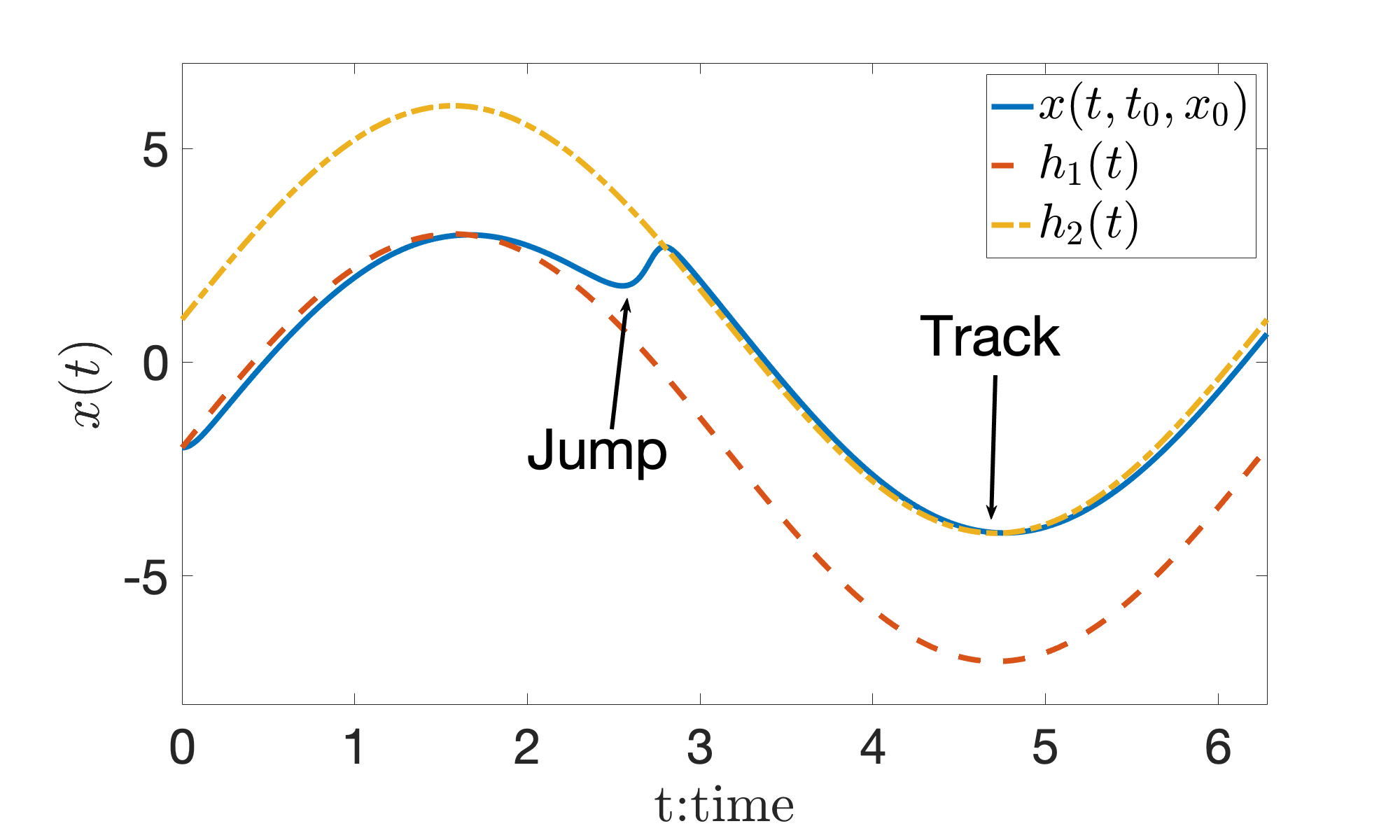
Figure 3 illustrates the definitions of jumping and tracking for Example 1 with and . The objective of this paper is to study when the solution of (P-ODE) started at a poor local minimum at the initial time jumps to and tracks a better (or global) minimum of the problem after some time. In other words, it is desirable to investigate the escaping property from and .
III Change of variables
Given two isolated local minimum trajectories , . One may use the change of variables to transform (P-ODE) into the form
| (24a) | ||||
| (24b) | ||||
We use to denote the solution of this differential equation starting at time with the initial point and use to denote the right-hand side of (24). Note that and are local solutions of (1) and as long as (1) is time-varying, these functions cannot satisfy (P-ODE) in general. We denote .
III-A Unconstrained optimization landscape after a change of variables
In this subsection, we study the unconstrained case to enable a better visualization of the optimization landscape. In the unconstrained case, (24) is reduced to
| (25) |
III-A1 Inertia encouraging the exploration
The first term in (25) can be understood as a time-varying gradient term that encourages the solution of (25) to track , while the second term represents the inertia from this trajectory. In particular, if points toward outside of the region of attraction of during some time interval, the term acts as an exploration term that encourages the solution of (ODE) to leave the region of attraction of . The parameter balances the roles of the gradient and the inertia.
In the extreme case where goes to infinity, converges to and approaches a constant trajectory determined by the initial point ; when is sufficiently small, the time-varying gradient term dominates the inertia term and the solution of (ODE) would track closely. With an appropriate proximal regularization that keeps the balance between the time-varying gradient term and the inertia term, the solution of (ODE) could temporarily track a local minimum trajectory with the potential of exploring other local minimum trajectories.
III-A2 Inertia creating a one-point strongly convex landscape
The differential equation (25) can be written as
| (26) |
This can be regarded as a time-varying gradient flow system of the original objective function plus a time-varying perturbation . During some time interval , the time-varying perturbation may enable the time-varying objective function over a neighborhood of to become one-point strongly convexified with respect to . Under such circumstances, the time-varying perturbation prompts the solution of (26) starting in a neighborhood of to move towards a neighborhood of . Before analyzing this phenomenon, we illustrate the concept in an example.
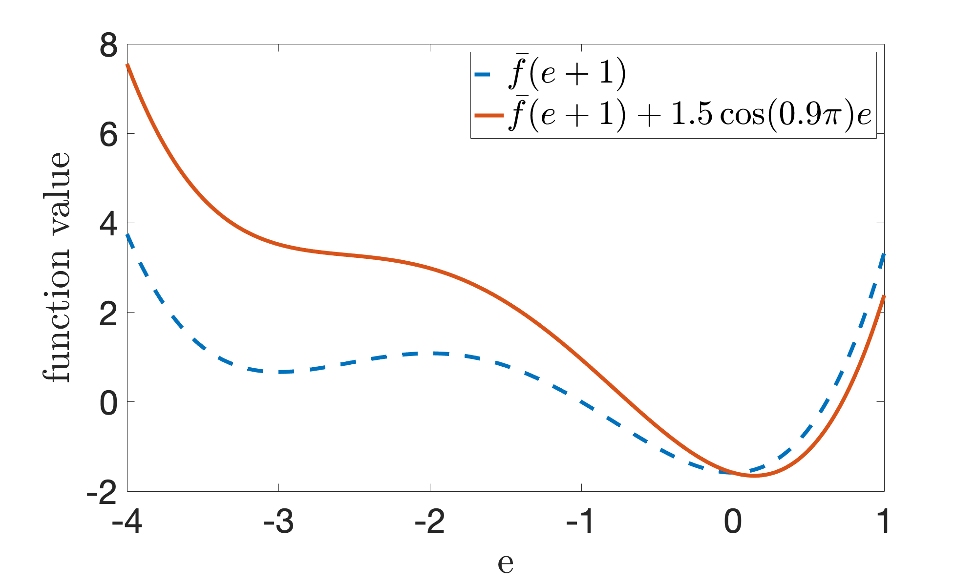
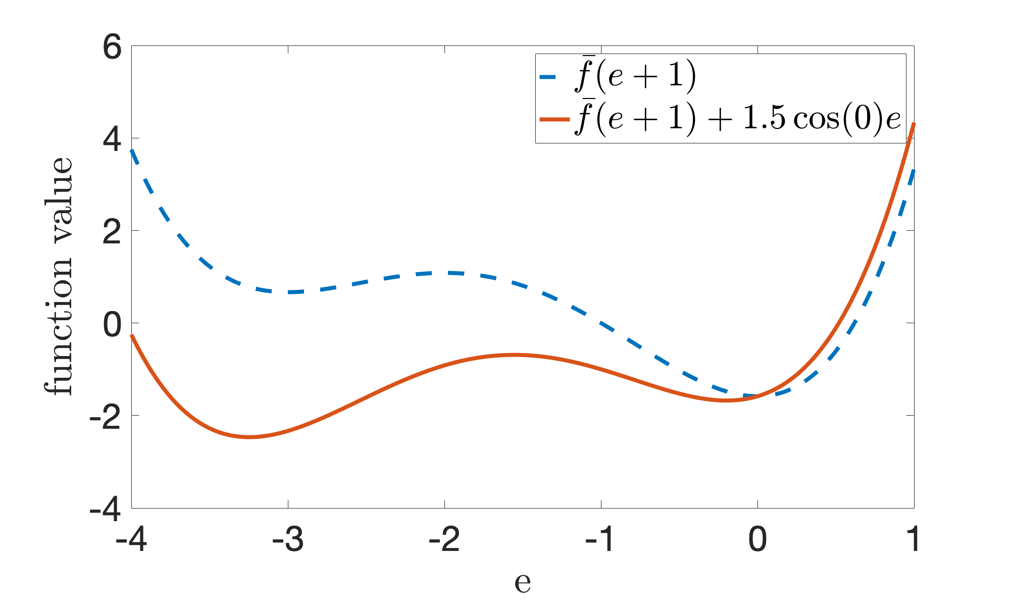
Consider again Example 1 and recall that has 2 local minima at and . By taking , and , the differential equation (26) can be expressed as . The landscape of the new time-varying function with the variable is shown for two cases and in Figure 4. The red curves are the solutions of (26) starting from . One can observe that when , the new landscape becomes one-point strongly convex around over the whole region for some time interval, which provides (26) with the opportunity of escaping from the region around to the region around . However, when , there are always two locally one-point strongly convex regions around and and, therefore, (26) fails to escape the region around .
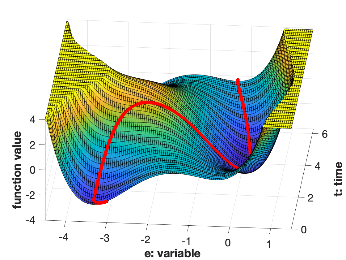
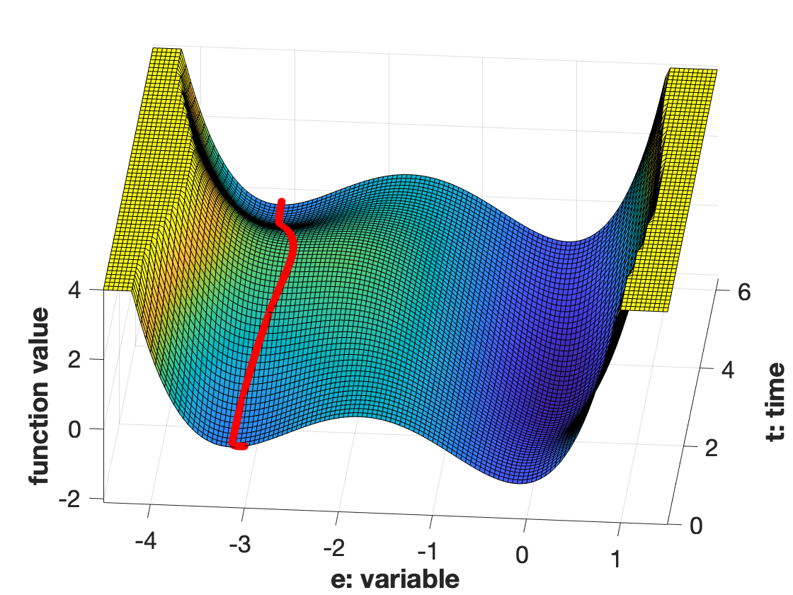
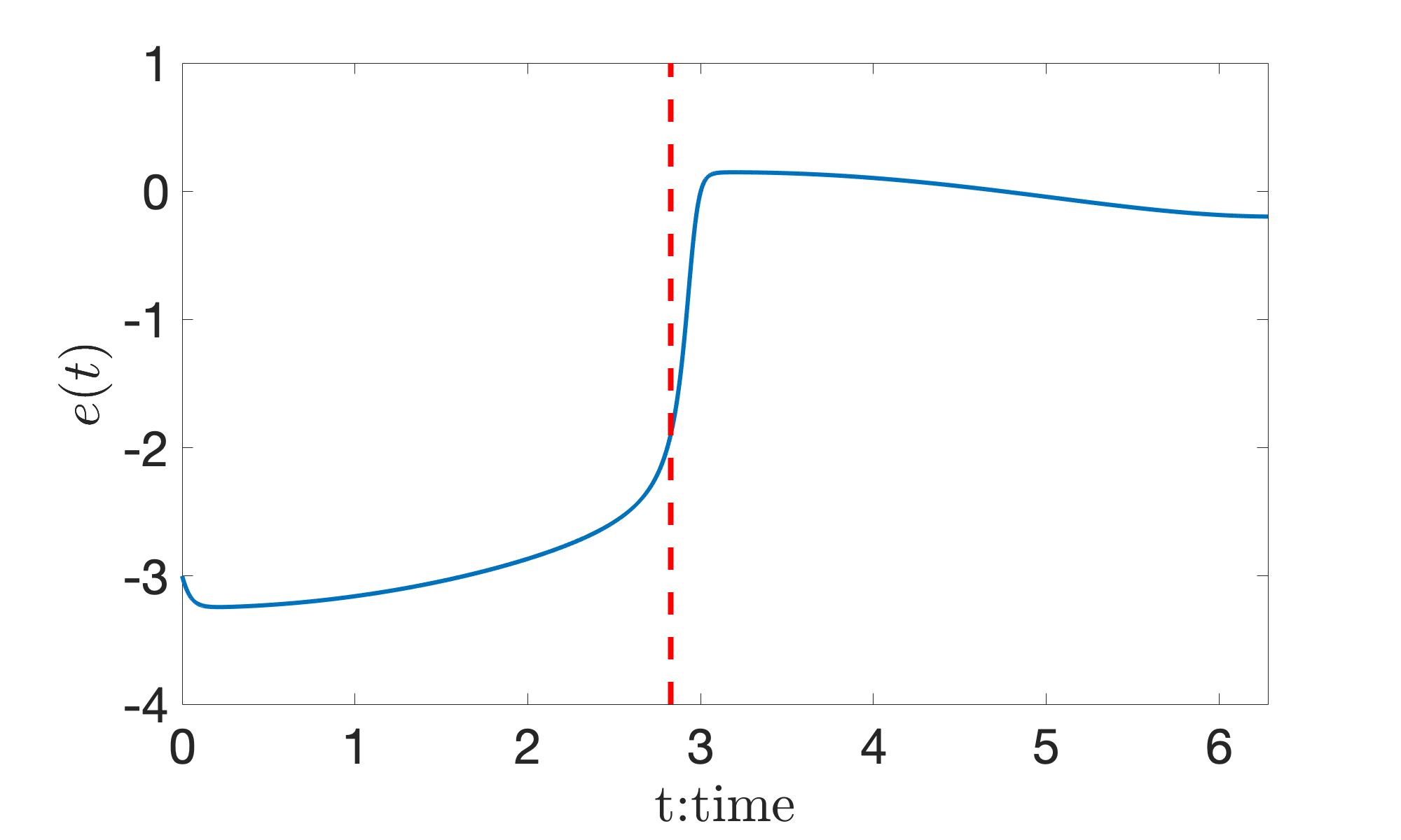
To further inspect the case , observe in Figure 5a that the landscape of the objective function shows that the region around the spurious local minimum trajectory is one-point strongly convexified with respect to at time . This is consistent with the fact that the solution of starting from jumps to the neighborhood of around time , as demonstrated in Figure 5c.
| Unconstrained problem | Equality-constrained problem | |
| First-order optimality condition(FOC) | ||
| ODE (continuous time limit of FOC for regularized problem) | ||
| Change of variables: | ||
| Key assumption: one-point strong convexity | ||
| Reshaping of the landscape: one-point strong convexification |
Furthermore, if the time interval is large enough to allow transitioning from a neighborhood of to a neighborhood of , then the solution of (26) would move to the neighborhood of . In contrast, the region around is never one-point strongly convexified with respect to , as shown in Figure 5b.
From the right-hand side of (26), it can be inferred that if the gradient of is relatively small around some local minimum trajectory, then its landscape is easier to be re-shaped by the time-varying linear perturbation . The local minimum trajectory in a neighborhood with small gradients usually corresponds to a shallow minimum trajectory in which the trajectory has a relatively flat landscape and a relatively small region of attraction. Thus, the one-point strong convexication introduced by the time-varying perturbation could help escape the shallow minimum trajectories.
III-B Dominant trajectory
In this subsection, we will formalize the intuitions discussed in Section III-A. We first define the notion of the shallow local minimum trajectory.
Definition 8.
Consider a positive number and assume that is -Lipschitz continuous. It is said that the local minimum trajectory is -shallow during the time period if and , where , , and is defined in (16).
In other words, a local minimum trajectory is shallow if it has a large time variation but a small region of attraction. We next show that whenever a local minimum trajectory is shallow during some time interval, the solution of (P-ODE) starting anywhere in the region of attraction of will leave its region of attraction at some time.
Lemma 4.
If the local minimum trajectory is -shallow during , then for any , then there exists a time such that .
Proof.
Let be the unit vector . One can write
For any and , we have
Hence,
The above contradiction completes the proof. ∎
On the one hand, Lemma 4 shows that any shallow local minimum trajectory is unstable in the sense that the time-variation in the minimum trajectory will force the solution of (P-ODE) to leave its region of attraction. If the shallow local minimum trajectory happens to be a non-global local solution, then the solution of (P-ODE), acting as a tracking algorithm, will help avoid the bad local solutions for free. On the other hand, Lemma 4 does not specify where the solution of (P-ODE) will end up after leaving the region of attraction of a shallow local minimum trajectory. Simulations (such as those provided in Sections III-A and V) suggest that, with some appropriate , the solution of (P-ODE) may move towards a nearby local minimum trajectory that has an enlarged region of one-point strong convexity. This leads to the following definition of the region of the domination and the dominant local minimum trajectory.
Definition 9.
Given two local minimum trajectories and , suppose that the time-varying Lagrange function with given in (3) is locally -one-point strongly convex with respect to around in the region . A set is said to be the region of domination for with respect to if it satisfies the following properties:
-
•
is a compact subset such that
(27) where is the solution of (24) staring from the feasible initial point at the initial time .
-
•
where
(28)
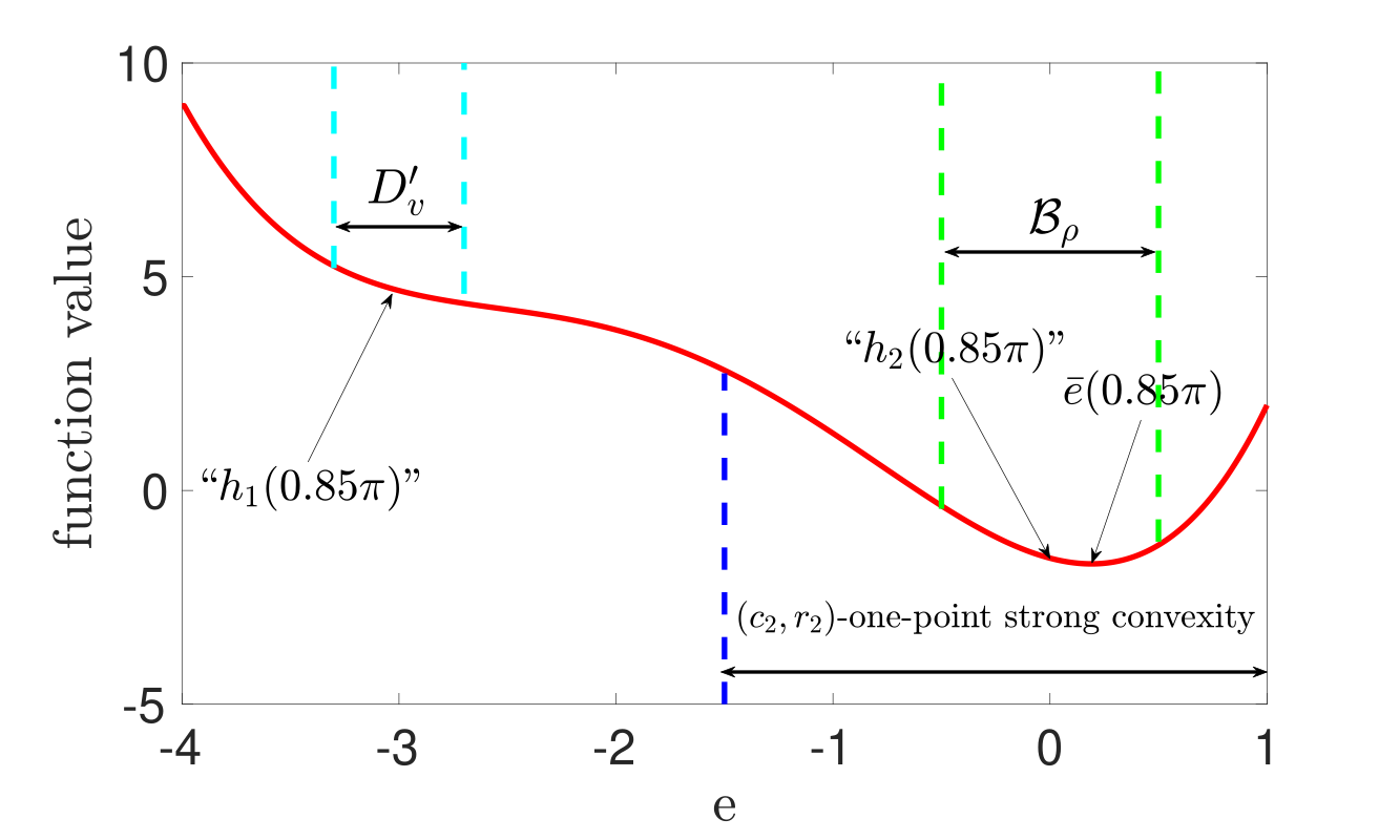
The condition (27) is a set invariance property, which requires that the solution of (24) starting from an initial point in stays in during the time period . For the visualization of , and in Definition 9, we consider again Example 1. In Fig 6, the red curve corresponds to the landscape of the function , corresponds to and corresponds to . is a region around containing all zeros of during a time period around and is a neighborhood around . In this example, the region of domination for with respect to is which contains and if if it also satisfies (27).
Definition 10.
It is said that is a -dominant trajectory with respect to during the time period over the region if the time variation of makes the time-varying function become one-point strongly monotone over , i.e.,
| (29) |
where is a constant and is defined in (28).
Note that being a dominant trajectory with respect to is equivalent to the statement that the inertia of creates a strongly convex landscape over , as discussed in Section III-A.
III-C The role of temporal variations of the constraints
From the perspective of the landscape of the Lagrange functional, (24b) can be regarded as a time-varying gradient flow system of the Lagrange functional plus a linear time-varying perturbation . Besides the linear time-varying perturbation induced by the inertia of the minimum trajectory similar to the unconstrained case, the constraints’ temporal variation plays the role of shifting the Lagrange multiplier from in (3) to in (15), which results in a nonlinear time-varying perturbation of the landscape of the Lagrange functional.
From the perspective of the perturbed gradient, the constraints’ temporal variation perturbs the projected gradient in an orthogonal direction to drive the trajectory of (24a) towards satisfying the time-varying constraints.
Lemma 5.
At any given time , the vector is orthogonal to the vector .
Proof.
Recall that is the orthogonal projection matrix on the tangent plane of at the point after the freezing time . Thus, we have . For the vector , it can be shown that
This implies that the orthogonal projection of the vector onto the tangent plane is . Thus, must be orthogonal to . ∎
Therefore, in the equality-constrained problem, the time-varying projected gradient flow system after a change of variables in (24a) can be regarded as a composition of a time-varying projected term , a time-varying constraint-driven term and an inertia term due to the time variation of the local minimum trajectory.
III-D A unified view for unconstrained and equality-constrained problems
By introducing the Lagrange functional in (5) and (16), we can unify the analysis of how the temporal variation and the proximal regularization help reshape the optimization landscape and potentially make the landscape become one-point strongly convex over a larger region, for both unconstrained and equality constrained problems. This unified view is illustrated in Table I.
IV Main results
In this section, we study the jumping, tracking and escaping properties for the time-varying nonconvex optimization.
IV-A Jumping
The following theorem shows that the solution of (P-ODE) could jump to the dominant trajectory as long as the time-interval of such domination is large enough.
Theorem 3 (Sufficient conditions for jumping from to ).
Suppose that the local minimum trajectory is a -dominant trajectory with respect to during over the region . Let be the initial point of (24), and consider defined in (28). Assume that is non-singular for all and and there exists a constant such that
| (30) |
Then, the solution of (P-ODE) will -jump from to over the time interval .
Proof.
First, notice that if is uniformly non-singular for all and , then defined in (28) is continuously differentiable for . Then, notice that every solution of (24) with an initial point in will remain in . It follows from Theorem 1 that (24) has a unique solution defined for all whenever .
We take as the Lyapunov function for the system (24). Because of Lemma 3, any solution of (24) stating in will remain in for all . Therefore, the derivative of along the trajectories of (24) in can be expressed as
| (31) |
where . By taking , since satisfies the condition (27), the solution of (24) starting from will stay in . Thus, the bound in (31) is valid. To ensure that the trajectory of (24) enters the time-varying set , it is sufficient to have or . Since . We can further bound as which is equivalent to .
Now, it is desirable to show that if the time interval is large enough, the solution of (24a) will enter the time-varying set with an exponential convergence rate. Since is negative in and because of (27), a trajectory starting from must stay in and move in a direction of decreasing . The function will continue decreasing until the trajectory enters the set or until time . Let us show that the trajectory enters before if . Since , (31) can be written as
By the comparison lemma[36, Lemma 3.4],
Hence,
The inequality holds if . ∎
We also offer an approach based on the time-averaged dynamics over a small time interval and name it “small interval averaging”222Our averaging approach distinguishes from classic averaging methods [37, 36, 49, 50] and the partial averaging method [51] in the sense that: (1) it is averaged over a small time interval instead of the entire time horizon, and (2) there is no two-time-scale behavior because there is no parameter in (25) that can be taken sufficiently small.. This technique guarantees that the solution of the time-varying differential equation (or system) will converge to a residual set of the origin of (25), provided that: (i) there is a time interval such that the temporal variation makes the averaged objective function during this interval locally one-point strongly convex around not only just over a neighborhood of but also over a neighborhood of , (ii) the original time-varying system is not too distant from the time-invariant averaged system, (iii) is large enough to allow the transition of points from a neighborhood of to a neighborhood of . Therefore, the time interval and the time-averaged dynamics over this time interval serve as a certificate for jumping from to . In what follows, we introduce the notion of averaging a time-varying function over a time interval .
Definition 11.
A function is said to be the average function of over the time interval if
The averaged system of (24) over the time interval can be written as
| (32) |
Then, (24) can be regarded as a time-invariant system (32) with the time-varying perturbation term . For the averaged system, we can define the on-average region of domination for with respect to similarly as Definition 9 by replacing (28) with
| (33) |
The corresponding on-average -dominant trajectory with respect to during over the region can also be defined similarly as Definition 10 by replacing (10) with
| (34) | ||||
where is defined in (33).
Theorem 4 (Sufficient conditions for jumping from to using averaging).
Suppose that the local minimum trajectory is a on-average -dominant trajectory with respect to during over the region . Assume that the following conditions are satisfied:
-
1.
There exist some time-varying scalar functions and such that
(35) for all , and there exist some positive constants and such that
(36) -
2.
The inequality
(37) holds, where and .
Then, the solution of (P-ODE) will -jump from to over the time interval .
Proof.
As shown in the proof of Theorem 3, the differential equation (24) has a unique solution defined for all that stays in whenever . By using as the Lyapunov function for the system (24), the derivative of along the trajectories of (24) can be obtained as
Since , one can derive an upper bound on as
To obtain a linear differential inequality, we consider . When , it holds that and
| (38) |
When , we have . Writing the Tylor expansion of for a sufficiently small yields that
This implies that
Therefore,
| (39) | ||||
Thus, (38) is also satisfied when , and accordingly satisfies (38) for all values of . Since is scalar and the right-hand side of (38) is continuous in and locally Lipschitz in for all and , the comparison lemma is applicable. In addition, the right-hand side of (38) is linear and a closed-form expression for the solution of the first-order linear differential equation of can be obtained. Hence, satisfies
| (40) |
where the translation function is given by
| (41) |
| (42) |
Since , and using and in (42), it holds that
| (43) |
By taking , since retains trajectories starting from a feasible initial point with respect to the dynamics (24) for , any trajectory of (24) starting from will stay in and remain in the feasible set . Thus, the bound in (IV-A) is valid. If satisfies
then . Since , we have . This shows that the solution of (25) jumps from to during the time interval . ∎
Remark 3.
Remark 4.
The condition in Theorem 3 and Condition 2 in Theorem 4 mean that needs to be large enough to allow the transition of points from a neighborhood of to a neighborhood of . Condition 1 in Theorem 4 means that the original time-varying system should not be too distant from the time-invariant averaged system.
Remark 5.
Remark 6.
Remark 7.
In Theorem 4, to ensure that the time-invariant partial interval averaged system is a reasonable approximation of the time-varying system, the time interval should not be very large. On the other hand, to guarantee that the solution of (24) has enough time to jump, the time interval should not be very small. This trade-off is reflected in (37).
IV-B Tracking
In this subsection, we study the tracking property of the local minimum trajectory . First, notice that if is not constant, the right-hand side of (P-ODE) is nonzero while the left-hand side is zero. Therefore, is not a solution of (P-ODE) in general. This is because the solution of (P-ODE) approximates the continuous limit of a discrete local trajectory of the sequential regularized optimization problem (10). However, to preserve the optimality of the solution with regards to the original time-varying optimization problem without any proximal regularization, it is required to guarantee that the solution of (P-ODE) is close to .
If the solution of (24) can be shown to be in a small residual set around on the time-varying manifold , then it is guaranteed that tracks its nearby local minimum trajectory. Notice that (24) can be regarded as a time-varying perturbation of the system
| (44) |
Since is a local minimum trajectory, it is obvious that is an equilibrium point of (44). In addition, if the time-varying Lagrange function with given in (3) is locally one-point strongly convex with respect to around in the time-varying feasible set , after noticing the fact that the solution of (24) will remain in if the initial point from Lemma 3, one would expect that the solution of (24) stays in a small residual set of if the perturbation is relatively small. The perturbation being small is equivalent to being small. The next theorem shows that every local minimum trajectory can be tracked for a relatively small .
Theorem 5 (Sufficient condition for tracking).
Assume that the time-varying Lagrange function with given in (3) is locally -one-point strongly convex with respect to around . Given such that , suppose that there exist time-varying scalar functions and such that the perturbed gradient due to the time-variation of constraints satisfies the inequality
| (45) |
and there exist some positive constants and such that
| (46) |
If is bounded and the following conditions hold
| (47a) | |||
| (47b) | |||
then the solution will -track . More specifically, we have
| (48) |
Proof.
Consider as the Lyapunov function for the system (24). Because of Lemma 3, any solution of (24) stating in will remain in for all . The derivative of along the trajectories of (24) can be obtained as
Since , one can derive an upper bound on as
Using the same proof procedure as in Theorem 4 and by taking and , it can be shown that
| (49) | ||||
To make the bound in (49) valid, we must ensure that for all . Note that
It can be verified that the condition will be satisfied if (47) holds. Furthermore, by and Theorem 1, there must exist a unique solution for (P-ODE) for all . ∎
Remark 8.
The inequality (5) implies that the smaller the regularization parameter is, the smaller the tracking error is and the faster converges to the neighbourhood of .
Remark 9.
In the case that the local minimum trajectory is a constant, the upper bound on simply becomes . This implies that if is constant, then it will be perfectly tracked with any regularization parameter and can not be escaped by tuning the regularization parameter.
Remark 10.
IV-C Escaping
Combining the results of jumping and tracking immediately yields a sufficient condition on escaping from one local minimum trajectory to a more desirable local (or global) minimum trajectory. The proof is omitted for brevity.
Theorem 6 (Sufficient conditions for escaping from to ).
Given two local minimum trajectories and , suppose that the Lagrange function with given in (3) is locally -one-point strongly convex with respect to around in the time-varying feasible set and let . Under the conditions of Theorem 3 or 4, if (45)-(47) hold, then the solution of (P-ODE) will -escape from to after .
IV-D Discussions
Adaptive inertia: To leverage the potential of the time-varying perturbation in re-shaping the landscape of the Langrange function or the objective function to become locally one-point strongly convex in over a large region, the regularization parameter should be selected relatively large. On the other hand, to ensure that the solution of (24) and (26) will end up tracking a desirable local (or global) minimum trajectory, Theorem 5 prescribes small values for . In practice, especially when the time-varying objective function has many spurious shallow minimum trajectories, this suggests using a relatively large regularization parameter at the beginning of the time horizon to escape spurious shallow minimum trajectories and then switching to a relative small regularization parameter for reducing the ultimate tracking error bound.
Sequential jumping: When the time-varying optimization problem has many local minimum trajectories, the solution of (P-ODE) or (ODE) may sequentially jump from one local minimum trajectory to a better local minimum trajectory. To illustrate this concept, consider the local minimum trajectories , where is a global trajectory. Assume that there exists a sequence of time intervals for such that the conditions of Theorem 3 or 4 are satisfied for and during each time interval. Then, by sequentially deploying Theorem 3 or 4, it can be concluded that the solution of (P-ODE) or (ODE) will jump from to after . Furthermore, if can be tracked with the given , the solution of (P-ODE) or (ODE) will escape from to after .
V Numerical Examples
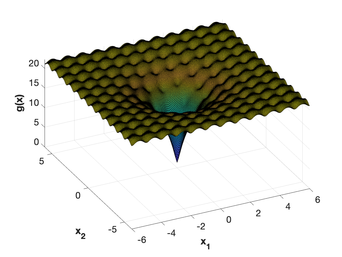
Example 3.
Consider the non-convex function
This function has a global minimum at with the optimal value and many spurious local minima. Its landscape is shown in Figure 7. When , this function is called the Ackley function [52], which is a benchmark function for global optimization algorithms. To make this function twice continuously differentiable, we choose .
Consider the time-varying objective function and the time-varying constraint , where . This constrained time-varying optimization problem has the global minimum trajectory and many spurious local minimum trajectories. Two local minimum trajectories are and . It can be shown that is locally -one-point strongly convex with respect to .
We take in Definition 10. The condition in (27) can be verified by checking the signs of the derivatives of and along the dynamics (24) on the boundary points of . Furthermore, (34) is satisfied for . Thus, is a -dominant trajectory with respect to during over the region .
Regarding Theorem 3, if we select , the inequality (37) is satisfied for and . Thus, the solution of (P-ODE) will -jump from to . Regarding Theorem 5, and in the inequality (45) can be taken as and , respectively. Then the inequality (47b) reduces to , which is satisfied by . Thus, the solution of (P-ODE) will -track . Putting the above findings together, we can conclude that the solution of (24) will -escape from to .
In addition, by choosing the inertia parameter , the simulation shows that for 1000 runs of random initialization with and determined by the equality constraint, all solutions of the corresponding (P-ODE) will sequentially jump over the local minimum trajectories and end up tracking the global trajectory after .
VI Conclusion
In this work, we study the landscape of time-varying nonconvex optimization problems. The objective is to understand when simple local search algorithms can find (and track) time-varying global solutions of the problem over time. We introduce a time-varying projected gradient flow system with controllable inertia as a continuous-time limit of the optimality conditions for discretized sequential optimization problems with proximal regularization and online updating scheme. Via a change of variables, the time-varying projected gradient flow system is regarded as a composition of a time-varying projected gradient term, a time-varying constraint-driven term and an inertia term due to the time variation of the local minimum trajectory. We show that the time-varying perturbation term due to the inertia encourages the exploration of the state space and re-shapes the landscape by potentially making it one-point strongly convex over a large region during some time interval. We introduce the notions of jumping and escaping, and use them to develop sufficient conditions under which the time-varying solution escapes from a poor local trajectory to a better (or global) minimum trajectory over a finite time interval. We illustrate in a benchmark example with many shallow minimum trajectories that the natural time variation of the problem enables escaping spurious local minima over time. Avenues for future work include the characterization of the class of problems in which all spurious local minimum trajectories are shallow compared with the global minimum trajectory.
Appendix A
Lemma 6.
Proof.
We first show that the matrix is positive definite over the time-varying feasible region for all . Since, under Assumption 3, is full row rank for for all , the null space of is . Thus, if and only if . Therefore, for all . Therefore, is positive definite. Denote as the minimum eigenvalue of . Then,there exists a positive constant such that . By the chain rule and the twice continuously differentiability of ’s in for , we know that is continuously differentiabile in for . Next, we show that is also continuously differentiabile in on . Let be the -th component of the vector . By taking the derivative of the identity with respect to , we obatin
and
Since the inversion operator is continuous by the Cayley–Hamilton theorem, is continuously differentiable in and is bounded, we know that is well-defined and continuous over for all . Therefore, is continuously differentiable in on . Consequently, and are continuously differentiable in on . Since is twice continuously differentiable in and ’s are twice continuously differentiable in for , it holds that the function is continuously differentiable in . Hence, because of [36, Theorem 3.2], it is locally Lipschitz continuous in on . ∎
Acknowledgment
This work was supported by grants from ARO, AFOSR, ONR and NSF.
References
- [1] Y. Ding, J. Lavaei, and M. Arcak, “Escaping spurious local minimum trajectories in online time-varying nonconvex optimization,” submitted for conference publication, 2020.
- [2] E. Hazan et al., “Introduction to online convex optimization,” Foundations and Trends® in Optimization, vol. 2, no. 3-4, pp. 157–325, 2016.
- [3] C. Jin, R. Ge, P. Netrapalli, S. M. Kakade, and M. I. Jordan, “How to escape saddle points efficiently,” in Proceedings of the 34th International Conference on Machine Learning-Volume 70. JMLR. org, 2017, pp. 1724–1732.
- [4] R. Ge, F. Huang, C. Jin, and Y. Yuan, “Escaping from saddle points—online stochastic gradient for tensor decomposition,” in Conference on Learning Theory, 2015, pp. 797–842.
- [5] R. Kleinberg, Y. Li, and Y. Yuan, “An alternative view: When does SGD escape local minima?” arXiv preprint arXiv:1802.06175, 2018.
- [6] K. Tanabe, “An algorithm for constrained maximization in nonlinear programming,” J. Oper. Res. Soc. Jpn, vol. 17, pp. 184–201, 1974.
- [7] J. Mulvaney-Kemp, S. Fattahi, and J. Lavaei, “Smoothing property of load variation promotes finding global solutions of time-varying optimal power flow,” https://lavaei.ieor.berkeley.edu/DOPF_2020_2.pdf, 2020.
- [8] Y. Tang, K. Dvijotham, and S. Low, “Real-time optimal power flow,” IEEE Transactions on Smart Grid, vol. 8, no. 6, pp. 2963–2973, 2017.
- [9] A. Hauswirth, I. Subotić, S. Bolognani, G. Hug, and F. Dörfler, “Time-varying projected dynamical systems with applications to feedback optimization of power systems,” in 2018 IEEE Conference on Decision and Control (CDC). IEEE, 2018, pp. 3258–3263.
- [10] C. V. Rao, J. B. Rawlings, and D. Q. Mayne, “Constrained state estimation for nonlinear discrete-time systems: Stability and moving horizon approximations,” IEEE Transactions on Automatic Control, vol. 48, no. 2, pp. 246–258, 2003.
- [11] T. Binder, L. Blank, H. G. Bock, R. Bulirsch, W. Dahmen, M. Diehl, T. Kronseder, W. Marquardt, J. P. Schlöder, and O. von Stryk, “Introduction to model based optimization of chemical processes on moving horizons,” in Online optimization of large scale systems. Springer, 2001, pp. 295–339.
- [12] M. Salman Asif and J. Romberg, “Sparse recovery of streaming signals using l1-homotopy,” arXiv preprint arXiv:1306.3331, 2013.
- [13] A. Balavoine, C. J. Rozell, and J. Romberg, “Discrete and continuous-time soft-thresholding with dynamic inputs,” arXiv preprint arXiv:1405.1361, 2014.
- [14] J. Kadam, W. Marquardt, M. Schlegel, T. Backx, O. Bosgra, P. Brouwer, G. Dünnebier, D. Van Hessem, A. Tiagounov, and S. De Wolf, “Towards integrated dynamic real-time optimization and control of industrial processes,” Proceedings foundations of computer-aided process operations (FOCAPO2003), pp. 593–596, 2003.
- [15] V. M. Zavala, E. M. Constantinescu, T. Krause, and M. Anitescu, “On-line economic optimization of energy systems using weather forecast information,” Journal of Process Control, vol. 19, no. 10, pp. 1725–1736, 2009.
- [16] A. Simonetto, A. Mokhtari, A. Koppel, G. Leus, and A. Ribeiro, “A class of prediction-correction methods for time-varying convex optimization,” IEEE Transactions on Signal Processing, vol. 64, no. 17, pp. 4576–4591, 2016.
- [17] M. Fazlyab, C. Nowzari, G. J. Pappas, A. Ribeiro, and V. M. Preciado, “Self-triggered time-varying convex optimization,” in 2016 IEEE 55th Conference on Decision and Control (CDC). IEEE, 2016, pp. 3090–3097.
- [18] A. Bernstein, E. Dall’Anese, and A. Simonetto, “Online primal-dual methods with measurement feedback for time-varying convex optimization,” IEEE Transactions on Signal Processing, vol. 67, no. 8, pp. 1978–1991, 2019.
- [19] A. Simonetto, “Time-varying convex optimization via time-varying averaged operators,” arXiv preprint arXiv:1704.07338, 2017.
- [20] J. Guddat, F. G. Vazquez, and H. T. Jongen, Parametric optimization: singularities, pathfollowing and jumps. Springer, 1990.
- [21] Y. Tang, E. Dall’Anese, A. Bernstein, and S. Low, “Running primal-dual gradient method for time-varying nonconvex problems,” arXiv preprint arXiv:1812.00613, 2018.
- [22] O. Massicot and J. Marecek, “On-line non-convex constrained optimization,” arXiv preprint arXiv:1909.07492, 2019.
- [23] S. Fattahi, C. Josz, R. Mohammadi, J. Lavaei, and S. Sojoudi, “Absence of spurious local trajectories in time-varying optimization,” arXiv preprint arXiv:1905.09937, 2019.
- [24] D. L. Donoho, “For most large underdetermined systems of linear equations the minimal -norm solution is also the sparsest solution,” Communications on Pure and Applied Mathematics: A Journal Issued by the Courant Institute of Mathematical Sciences, vol. 59, no. 6, pp. 797–829, 2006.
- [25] E. J. Candes and Y. Plan, “Matrix completion with noise,” Proceedings of the IEEE, vol. 98, no. 6, pp. 925–936, 2010.
- [26] E. J. Candès and B. Recht, “Exact matrix completion via convex optimization,” Foundations of Computational Mathematics, vol. 9, no. 6, p. 717, 2009.
- [27] H. Li, Z. Xu, G. Taylor, C. Studer, and T. Goldstein, “Visualizing the loss landscape of neural nets,” in Advances in Neural Information Processing Systems, 2018, pp. 6389–6399.
- [28] J. Lavaei and S. H. Low, “Zero duality gap in optimal power flow problem,” IEEE Transactions on Power Systems, vol. 27, no. 1, pp. 92–107, 2012.
- [29] J. D. Lee, I. Panageas, G. Piliouras, M. Simchowitz, M. I. Jordan, and B. Recht, “First-order methods almost always avoid saddle points,” arXiv preprint arXiv:1710.07406, 2017.
- [30] S. Bhojanapalli, B. Neyshabur, and N. Srebro, “Global optimality of local search for low rank matrix recovery,” in Advances in Neural Information Processing Systems, 2016, pp. 3873–3881.
- [31] R. Ge, J. D. Lee, and T. Ma, “Matrix completion has no spurious local minimum,” in Advances in Neural Information Processing Systems, 2016, pp. 2973–2981.
- [32] R. Y. Zhang, S. Sojoudi, and J. Lavaei, “Sharp restricted isometry bounds for the inexistence of spurious local minima in nonconvex matrix recovery,” Journal of Machine Learning Research, 2019.
- [33] S. Fattahi and S. Sojoudi, “Exact guarantees on the absence of spurious local minima for non-negative robust principal component analysis,” arXiv preprint arXiv:1812.11466, 2018.
- [34] C. Josz, Y. Ouyang, R. Zhang, J. Lavaei, and S. Sojoudi, “A theory on the absence of spurious solutions for nonconvex and nonsmooth optimization,” in Advances in Neural Information Processing Systems, 2018, pp. 2441–2449.
- [35] J. Sun, Q. Qu, and J. Wright, “Complete dictionary recovery over the sphere I: Overview and the geometric picture,” IEEE Transactions on Information Theory, vol. 63, no. 2, pp. 853–884, 2016.
- [36] H. K. Khalil, Nonlinear systems. Upper Saddle River, 2002.
- [37] J. K. Hale, Ordinary differential equations. Wiley-Inter-science, 1980.
- [38] W. Su, S. Boyd, and E. Candes, “A differential equation for modeling nesterov’s accelerated gradient method: Theory and insights,” in Advances in Neural Information Processing Systems, 2014, pp. 2510–2518.
- [39] W. Krichene, A. Bayen, and P. L. Bartlett, “Accelerated mirror descent in continuous and discrete time,” in Advances in Neural Information Processing Systems, 2015, pp. 2845–2853.
- [40] A. Wibisono, A. C. Wilson, and M. I. Jordan, “A variational perspective on accelerated methods in optimization,” Proceedings of the National Academy of Sciences, vol. 113, no. 47, pp. E7351–E7358, 2016.
- [41] A. M. Saxe, J. L. McClelland, and S. Ganguli, “Exact solutions to the nonlinear dynamics of learning in deep linear neural networks,” arXiv preprint arXiv:1312.6120, 2013.
- [42] S. Gunasekar, B. E. Woodworth, S. Bhojanapalli, B. Neyshabur, and N. Srebro, “Implicit regularization in matrix factorization,” in Advances in Neural Information Processing Systems, 2017, pp. 6151–6159.
- [43] D. P. Bertsekas, Nonlinear programming. Athena Scientific, 2016.
- [44] A. Sard, “The measure of the critical values of differentiable maps,” Bulletin of the American Mathematical Society, vol. 48, no. 12, pp. 883–890, 1942.
- [45] G. Still, “Lectures on parametric optimization: An introduction,” Optimization Online, 2018.
- [46] J. Rosen, “The gradient projection method for nonlinear programming. part ii. nonlinear constraints,” Journal of the Society for Industrial and Applied Mathematics, vol. 9, no. 4, pp. 514–532, 1961.
- [47] D. G. Luenberger, “The gradient projection method along geodesics,” Management Science, vol. 18, no. 11, pp. 620–631, 1972.
- [48] A. Iserles, A first course in the numerical analysis of differential equations. Cambridge University Press, 2009, no. 44.
- [49] A. R. Teel, J. Peuteman, and D. Aeyels, “Semi-global practical asymptotic stability and averaging,” Systems & Control Letters, vol. 37, no. 5, pp. 329–334, 1999.
- [50] D. Aeyels and J. Peuteman, “On exponential stability of nonlinear time-varying differential equations,” Automatica, vol. 35, no. 6, pp. 1091–1100, 1999.
- [51] J. Peuteman and D. Aeyels, “Exponential stability of nonlinear time-varying differential equations and partial averaging,” Mathematics of Control, Signals and Systems, vol. 15, no. 1, pp. 42–70, 2002.
- [52] D. H. Ackley, A Connectionist Machine for Genetic Hillclimbing. Norwell, MA, USA: Kluwer Academic Publishers, 1987.
![[Uncaptioned image]](/html/1912.00561/assets/photo_Yuhao.jpeg) |
Yuhao Ding is currently working toward the Ph.D. degree in Industrial Engineering and Operations Research at the University of California, Berkeley, CA, USA. He obtained the B.E. degree in Aerospace Engineering from Nanjing University of Aeronautics and Astronautics in 2016, and the M.S. degree in Electrical and Computer Engineering from University of Michigan, Ann Arbor in 2018. |
![[Uncaptioned image]](/html/1912.00561/assets/Photo_Lavaei.jpg) |
Javad Lavaei is currently an Associate Professor in the Department of Industrial Engineering and Operations Research at the University of California, Berkeley, CA, USA. He has worked on different interdisciplinary problems in power systems, optimization theory, control theory, and data science. He is an associate editor of the IEEE Transactions on Automatic Control, the IEEE Transactions on Smart Grid, and the IEEE Control System Letters. He serves on the conference editorial boards of the IEEE Control Systems Society and European Control Association. |
![[Uncaptioned image]](/html/1912.00561/assets/photo_arcak.jpg) |
Murat Arcak is currently a Professor with the Department of Electrical Engineering and Computer Sciences, University of California, Berkeley, CA, USA. His research interests include dynamical systems and control theory with applications to synthetic biology, multiagent systems, and transportation. Prof. Arcak was a recipient of the CAREER Award from the National Science Foundation in 2003, the Donald P. Eckman Award from the American Automatic Control Council in 2006, the Control and Systems Theory Prize from the Society for Industrial and Applied Mathematics (SIAM) in 2007, and the Antonio Ruberti Young Researcher Prize from the IEEE Control Systems Society in 2014. He is a member of SIAM. |