Risk Bounds for Low Cost Bipartite Ranking

San Gultekin and John Paisley
Abstract

Bipartite ranking is an important supervised learning problem; however, unlike regression or classification, it has a quadratic dependence on the number of samples. To circumvent the prohibitive sample cost, many recent work focus on stochastic gradient-based methods. In this paper we consider an alternative approach, which leverages the structure of the widely-adopted pairwise squared loss, to obtain a stochastic and low cost algorithm that does not require stochastic gradients or learning rates. Using a novel uniform risk bound—based on matrix and vector concentration inequalities—we show that the sample size required for competitive performance against the all-pairs batch algorithm does not have a quadratic dependence. Generalization bounds for both the batch and low cost stochastic algorithms are presented. Experimental results show significant speed gain against the batch algorithm, as well as competitive performance against state-of-the-art bipartite ranking algorithms on real datasets.

1 Introduction

Binary classification is among the most widely studied machine learning problems, with many applications. Given a binary labeled dataset, the aim is to learn a mapping from the features to the labels. The performance of a learning algorithm is typically gauged in terms of classification error. However, in situations such as cost-sensitive learning [1] and imbalanced learning [2, 3] this choice may not be appropriate. For example, in online advertising [1] one is typically concerned with separating the interesting ads from the rest. This problem is also known as bipartite ranking, where the aim is to rank the “positive” inputs higher than the “negative” ones.

1.1 Problem Setup

Let 𝒳𝒳\mathcal{X} be a D𝐷D-dimensional input domain and 𝒴𝒴\mathcal{Y} the label domain. The bipartite ranking problem is defined for binary labeled samples, 𝒴={0,1}𝒴01\mathcal{Y}=\{0,1\}. These sample pairs are generated i.i.d. from an unknown distribution 𝒟𝒟\mathcal{D} on 𝒳×𝒴𝒳𝒴\mathcal{X}\times\mathcal{Y}. A ranking function f:𝒳:𝑓𝒳f:\mathcal{X}\rightarrow\mathbb{R} is a mapping from the inputs to a scalar-valued score. In this paper we are interested in linear ranking functions of the form f(𝐱)=𝐰𝐱𝑓𝐱superscript𝐰top𝐱f(\mathbf{x})=\mathbf{w}^{\top}\mathbf{x} with parameter vector 𝐰𝐰\mathbf{w}. The goal in bipartite ranking is to assign higher scores to the inputs with label 1. Let 𝐱1superscript𝐱1\mathbf{x}^{1} and 𝐱0superscript𝐱0\mathbf{x}^{0} denote two samples with corresponding labels of 111 and 00. In many ranking settings we are given a set of features that encodes the preference of one sample over another [1], which can be represented by Ψ(𝐱1,𝐱0)Ψsuperscript𝐱1superscript𝐱0\Psi(\mathbf{x}^{1},\mathbf{x}^{0}). It is also possible that the individual features 𝐱0subscript𝐱0\mathbf{x}_{0} and 𝐱1subscript𝐱1\mathbf{x}_{1} are not defined explicitly; for example when a single user is shown two ads and prefers one over another. Given this, a widely used performance metric is the Wilcoxon-Mann-Whitney statistic

WMW(𝐰,Ψ(𝐱1,𝐱0))=𝕀{𝐰Ψ(𝐱1,𝐱0)>0}+12𝕀{𝐰Ψ(𝐱1,𝐱0)=0}.subscriptWMW𝐰Ψsuperscript𝐱1superscript𝐱0𝕀superscript𝐰topΨsuperscript𝐱1superscript𝐱0012𝕀superscript𝐰topΨsuperscript𝐱1superscript𝐱00\displaystyle\mathbf{\ell}_{\text{WMW}}(\mathbf{w},\Psi(\mathbf{x}^{1},\mathbf{x}^{0}))=\mathbb{I}\left\{\mathbf{w}^{\top}\Psi(\mathbf{x}^{1},\mathbf{x}^{0})>0\right\}+\frac{1}{2}\mathbb{I}\left\{\mathbf{w}^{\top}\Psi(\mathbf{x}^{1},\mathbf{x}^{0})=0\right\}~{}. (1)

Based on this we define the risks

RAUC(𝐰)=𝔼x1D1x0D0[WMW(𝐰,Ψ(𝐱1,𝐱0))],R𝒩AUC(𝐰)=1N1N0i=1N1j=1N0WMW(𝐰,Ψ(𝐱i1,𝐱j0)),formulae-sequencesuperscript𝑅AUC𝐰subscript𝔼similar-tosuperscript𝑥1superscript𝐷1similar-tosuperscript𝑥0superscript𝐷0delimited-[]subscriptWMW𝐰Ψsuperscript𝐱1superscript𝐱0subscriptsuperscript𝑅AUC𝒩𝐰1subscript𝑁1subscript𝑁0superscriptsubscript𝑖1subscript𝑁1superscriptsubscript𝑗1subscript𝑁0subscriptWMW𝐰Ψsuperscriptsubscript𝐱𝑖1superscriptsubscript𝐱𝑗0\displaystyle R^{\text{\tiny AUC}}(\mathbf{w})=\mathbb{E}_{\begin{subarray}{c}x^{1}\sim D^{1}\\ x^{0}\sim D^{0}\end{subarray}}\left[\mathbf{\ell}_{\text{WMW}}(\mathbf{w},\Psi(\mathbf{x}^{1},\mathbf{x}^{0}))\right],~{}~{}R^{\text{\tiny AUC}}_{\mathcal{N}}(\mathbf{w})=\frac{1}{N_{1}N_{0}}\sum_{i=1}^{N_{1}}\sum_{j=1}^{N_{0}}\mathbf{\ell}_{\text{WMW}}(\mathbf{w},\Psi(\mathbf{x}_{i}^{1},\mathbf{x}_{j}^{0})), (2)

where RAUC(𝐰)superscript𝑅AUC𝐰R^{\text{\tiny AUC}}(\mathbf{w}) corresponds to the actual AUC risk and is obtained by taking expectation over the class-conditional distributions Di=D(𝐱|y=i)superscript𝐷𝑖𝐷conditional𝐱𝑦𝑖D^{i}=D(\mathbf{x}|y=i). Let the sample set 𝒩={𝐱10,,𝐱N00,𝐱11,,𝐱N11}𝒩superscriptsubscript𝐱10superscriptsubscript𝐱subscript𝑁00superscriptsubscript𝐱11superscriptsubscript𝐱subscript𝑁11\mathcal{N}=\{\mathbf{x}_{1}^{0},\ldots,\mathbf{x}_{N_{0}}^{0},\mathbf{x}_{1}^{1},\ldots,\mathbf{x}_{N_{1}}^{1}\}, containing N0subscript𝑁0N_{0} and N1subscript𝑁1N_{1} samples with labels 0 and 1, respectively, and define N:=N0+N1assign𝑁subscript𝑁0subscript𝑁1N:=N_{0}+N_{1}. This gives the empirical risk R𝒩AUC(𝐰)subscriptsuperscript𝑅AUC𝒩𝐰R^{\text{\tiny AUC}}_{\mathcal{N}}(\mathbf{w}) to be minimized in practice. The main drawback of this approach is that the objective function is now a sum of indicator functions, an NP-hard problem. A widely-used approach to handle this problem is to replace the intrinsic loss function WMWsubscriptWMW\mathbf{\ell}_{\text{WMW}} with a convex one, often written as ϕsubscriptitalic-ϕ\mathbf{\ell}_{\phi} [4, 5].

In this paper we are interested in the pairwise squared loss as it is a consistent estimator of AUC [6], and widely preferred by recent work [7, 8, 9]:

ϕ(𝐰,(𝐱1,𝐱0))=12[1𝐰Ψ(𝐱i1,𝐱j0)]2,subscriptitalic-ϕ𝐰superscript𝐱1superscript𝐱012superscriptdelimited-[]1superscript𝐰topΨsuperscriptsubscript𝐱𝑖1superscriptsubscript𝐱𝑗02\displaystyle\mathbf{\ell}_{\phi}(\mathbf{w},(\mathbf{x}^{1},\mathbf{x}^{0}))=\frac{1}{2}\left[1-\mathbf{w}^{\top}\Psi(\mathbf{x}_{i}^{1},\mathbf{x}_{j}^{0})\right]^{2}, (3)

which produces its own corresponding actual and empirical ϕitalic-ϕ\phi-risks that parallels Eq. (2). Let 𝚺N=1/(N1N0)i=1N1j=1N0Ψ(𝐱i1,𝐱j0)Ψ(𝐱i1,𝐱j0)subscript𝚺𝑁1subscript𝑁1subscript𝑁0superscriptsubscript𝑖1subscript𝑁1superscriptsubscript𝑗1subscript𝑁0Ψsuperscriptsubscript𝐱𝑖1superscriptsubscript𝐱𝑗0Ψsuperscriptsuperscriptsubscript𝐱𝑖1superscriptsubscript𝐱𝑗0top\mathbf{\Sigma}_{N}=1/(N_{1}N_{0})\sum_{i=1}^{N_{1}}\sum_{j=1}^{N_{0}}\Psi(\mathbf{x}_{i}^{1},\mathbf{x}_{j}^{0})\Psi(\mathbf{x}_{i}^{1},\mathbf{x}_{j}^{0})^{\top} and μN=1/(N1N0)i=1N1j=1N0Ψ(𝐱i1,𝐱j0)subscript𝜇𝑁1subscript𝑁1subscript𝑁0superscriptsubscript𝑖1subscript𝑁1superscriptsubscript𝑗1subscript𝑁0Ψsuperscriptsubscript𝐱𝑖1superscriptsubscript𝐱𝑗0\mathbf{\mu}_{N}=1/(N_{1}N_{0})\sum_{i=1}^{N_{1}}\sum_{j=1}^{N_{0}}\Psi(\mathbf{x}_{i}^{1},\mathbf{x}_{j}^{0}). The empirical risk for this problem can then also written as the optimization of R𝒩ϕ(𝐰)=(1/2)𝐰𝚺N𝐰μN𝐰superscriptsubscript𝑅𝒩italic-ϕ𝐰12superscript𝐰topsubscript𝚺𝑁𝐰superscriptsubscript𝜇𝑁top𝐰R_{\mathcal{N}}^{\phi}(\mathbf{w})=(1/2)\mathbf{w}^{\top}\mathbf{\Sigma}_{N}\mathbf{w}-\mathbf{\mu}_{N}^{\top}\mathbf{w}. For what follows we will drop the ϕitalic-ϕ\phi symbol and refer to ϕsubscriptitalic-ϕ\mathbf{\ell}_{\phi}, Rϕsuperscript𝑅italic-ϕR^{\phi}, and R𝒩ϕsuperscriptsubscript𝑅𝒩italic-ϕR_{\mathcal{N}}^{\phi} simply as \mathbf{\ell}, R𝑅R, and R𝒩subscript𝑅𝒩R_{\mathcal{N}}.

The focus of this paper is on two algorithms: The first one is a Batch Bipartite Ranking (BBR) algorithm (Algorithm 1), which aims at minimizing R𝒩subscript𝑅𝒩R_{\mathcal{N}} based on all pairs available in 𝒩𝒩\mathcal{N}. We provide a new theoretical analysis of BBR in Section 2. Due to the quadratic growth of sample size, O(N1N0)𝑂subscript𝑁1subscript𝑁0O(N_{1}N_{0}), the sample cost of BBR quickly becomes prohibitive. Therefore we also propose a new Low Cost Bipartite Ranking (LCBR) algorithm (Algorithm 2), which, given the same sample set 𝒩𝒩\mathcal{N}, subsamples S𝑆S pairs uniformly at random with replacement. The main goal of this paper is to analyze the subsample size S𝑆S required for LCBR to be competitive with BBR. As we show in Section 3, S𝑆S does not have such quadratic dependence. Section 4 discusses related work. We show experiments in Section 5 and conclude in Section 6.

Algorithm 1 BBR

Input:    Sample set 𝒩𝒩\mathcal{N}
Input:    Regularization parameter (Wsubscript𝑊W_{*})
Output: Linear ranker’s weight 𝐰Nsubscript𝐰𝑁\mathbf{w}_{N}
1. Initialize μN𝟎subscript𝜇𝑁0\mathbf{\mu}_{N}\leftarrow\mathbf{0}, 𝚺N𝟎subscript𝚺𝑁0\mathbf{\Sigma}_{N}\leftarrow\mathbf{0}
2. //Accummulation
3. for i=1,,N1𝑖1subscript𝑁1i=1,\ldots,N_{1}
4.   for j=1,,N0𝑗1subscript𝑁0j=1,\ldots,N_{0}
5.    μNμN+1N1N0(𝐱i1𝐱j0)subscript𝜇𝑁subscript𝜇𝑁1subscript𝑁1subscript𝑁0superscriptsubscript𝐱𝑖1superscriptsubscript𝐱𝑗0\mathbf{\mu}_{N}\leftarrow\mathbf{\mu}_{N}+\frac{1}{N_{1}N_{0}}(\mathbf{x}_{i}^{1}-\mathbf{x}_{j}^{0})
6.    𝚺N𝚺N+1N1N0(𝐱i1𝐱j0)(𝐱i1𝐱j0)subscript𝚺𝑁subscript𝚺𝑁1subscript𝑁1subscript𝑁0superscriptsubscript𝐱𝑖1superscriptsubscript𝐱𝑗0superscriptsuperscriptsubscript𝐱𝑖1superscriptsubscript𝐱𝑗0top\mathbf{\Sigma}_{N}\leftarrow\mathbf{\Sigma}_{N}+\frac{1}{N_{1}N_{0}}(\mathbf{x}_{i}^{1}-\mathbf{x}_{j}^{0})(\mathbf{x}_{i}^{1}-\mathbf{x}_{j}^{0})^{\top}
7.   end for
8. end for
9. //Empirical Risk Minimization
10. 𝐰Nargmin𝐰B2(W)12𝐰𝚺N𝐰μN𝐰subscript𝐰𝑁𝐰subscript𝐵2subscript𝑊12superscript𝐰topsubscript𝚺𝑁𝐰superscriptsubscript𝜇𝑁top𝐰\mathbf{w}_{N}\leftarrow\underset{\mathbf{w}\in B_{2}(W_{*})}{\arg\min}~{}~{}\frac{1}{2}\mathbf{w}^{\top}\mathbf{\Sigma}_{N}\mathbf{w}-\mathbf{\mu}_{N}^{\top}\mathbf{w}

Algorithm 2 LCBR

Input:    Sample set 𝒩𝒩\mathcal{N}, subsample size (S𝑆S)
Input:    Regularization parameter (Wsubscript𝑊W_{*})
Output: Linear ranker’s weight 𝐰Ssubscript𝐰𝑆\mathbf{w}_{S}
1. Initialize μS𝟎subscript𝜇𝑆0\mathbf{\mu}_{S}\leftarrow\mathbf{0}, 𝚺S𝟎subscript𝚺𝑆0\mathbf{\Sigma}_{S}\leftarrow\mathbf{0}
2. //Accummulation
3. for s=1,,S𝑠1𝑆s=1,\ldots,S
4.   Sample (is,js)subscript𝑖𝑠subscript𝑗𝑠(i_{s},j_{s}) uniformly with replacement
5.   μSμS+1S(𝐱is1𝐱js0)subscript𝜇𝑆subscript𝜇𝑆1𝑆superscriptsubscript𝐱subscript𝑖𝑠1superscriptsubscript𝐱subscript𝑗𝑠0\mathbf{\mu}_{S}\leftarrow\mathbf{\mu}_{S}+\frac{1}{S}(\mathbf{x}_{i_{s}}^{1}-\mathbf{x}_{j_{s}}^{0})
6.   𝚺S𝚺S+1S(𝐱is1𝐱js0)(𝐱is1𝐱js0)subscript𝚺𝑆subscript𝚺𝑆1𝑆superscriptsubscript𝐱subscript𝑖𝑠1superscriptsubscript𝐱subscript𝑗𝑠0superscriptsuperscriptsubscript𝐱subscript𝑖𝑠1superscriptsubscript𝐱subscript𝑗𝑠0top\mathbf{\Sigma}_{S}\leftarrow\mathbf{\Sigma}_{S}+\frac{1}{S}(\mathbf{x}_{i_{s}}^{1}-\mathbf{x}_{j_{s}}^{0})(\mathbf{x}_{i_{s}}^{1}-\mathbf{x}_{j_{s}}^{0})^{\top}
7. end for
8. end for
9. //Empirical Risk Minimization
10. 𝐰Sargmin𝐰B2(W)12𝐰𝚺S𝐰μS𝐰subscript𝐰𝑆𝐰subscript𝐵2subscript𝑊12superscript𝐰topsubscript𝚺𝑆𝐰superscriptsubscript𝜇𝑆top𝐰\mathbf{w}_{S}\leftarrow\underset{\mathbf{w}\in B_{2}(W_{*})}{\arg\min}~{}~{}\frac{1}{2}\mathbf{w}^{\top}\mathbf{\Sigma}_{S}\mathbf{w}-\mathbf{\mu}_{S}^{\top}\mathbf{w}

Remark: At this point, for the ease of presentation we focus on the case Ψ(𝐱i1,𝐱j0)=𝐱i1𝐱j0Ψsuperscriptsubscript𝐱𝑖1superscriptsubscript𝐱𝑗0superscriptsubscript𝐱𝑖1superscriptsubscript𝐱𝑗0\Psi(\mathbf{x}_{i}^{1},\mathbf{x}_{j}^{0})=\mathbf{x}_{i}^{1}-\mathbf{x}_{j}^{0} (which is reflected in Algorithms 1 and 2). All the theory developed in this paper is valid for the most general case of Ψ(𝐱i1,𝐱j0)Ψsuperscriptsubscript𝐱𝑖1superscriptsubscript𝐱𝑗0\Psi(\mathbf{x}_{i}^{1},\mathbf{x}_{j}^{0}), however. In particular, imposing a norm bound on the individual features 𝐱i1,𝐱j0superscriptsubscript𝐱𝑖1superscriptsubscript𝐱𝑗0\mathbf{x}_{i}^{1},\mathbf{x}_{j}^{0} is equivalent to imposing a scaled norm bound on Ψ(𝐱i1,𝐱j0)Ψsuperscriptsubscript𝐱𝑖1superscriptsubscript𝐱𝑗0\Psi(\mathbf{x}_{i}^{1},\mathbf{x}_{j}^{0}).

Additional assumptions: We assume the input domain is compact, 𝒳2(X)𝒳subscript2subscript𝑋\mathcal{X}\subseteq\mathcal{B}_{2}(X_{*}) which implies 𝐱2Xsubscriptnorm𝐱2subscript𝑋\left\|\mathbf{x}\right\|_{2}\leq X_{*}, and that the domain of ranking functions is compact, taking 𝒲=2(W)𝒲subscript2subscript𝑊\mathcal{W}=\mathcal{B}_{2}(W_{*}) such that 𝐰2Wsubscriptnorm𝐰2subscript𝑊\left\|\mathbf{w}\right\|_{2}\leq W_{*}. Here p(r):={𝐱𝒳:𝐱pr}assignsubscript𝑝𝑟conditional-set𝐱𝒳subscriptnorm𝐱𝑝𝑟\mathcal{B}_{p}(r):=\{\mathbf{x}\in\mathcal{X}:\left\|\mathbf{x}\right\|_{p}\leq r\} is the psubscript𝑝\ell_{p}-ball of radius r𝑟r. The first assumption is related to data preprocessing where the features are scaled appropriately; the second assumption corresponds to regularization. For both cases we chose the 2subscript2\ell_{2}-norm as it provides a dimension-independent upper bound; however it is still possible to derive bounds using other norms. Let 𝐰Nsubscript𝐰𝑁\mathbf{w}_{N} and 𝐰Ssubscript𝐰𝑆\mathbf{w}_{S} be the minimizer of the empirical risk objectives (Algorithms 1 and 2, Line 10). Also for clarity we focus on the case where 𝚺,𝚺N,𝚺S𝟎succeeds𝚺subscript𝚺𝑁subscript𝚺𝑆0\mathbf{\Sigma},\mathbf{\Sigma}_{N},\mathbf{\Sigma}_{S}\succ\mathbf{0} in the sequel.111Where we defined 𝚺=𝔼𝐱1P1,𝐱0P0[(𝐱1𝐱0)(𝐱1𝐱0)]𝚺subscript𝔼formulae-sequencesimilar-tosubscript𝐱1subscript𝑃1similar-tosubscript𝐱0subscript𝑃0delimited-[]subscript𝐱1subscript𝐱0superscriptsubscript𝐱1subscript𝐱0top\mathbf{\Sigma}=\mathbb{E}_{\mathbf{x}_{1}\sim P_{1},\mathbf{x}_{0}\sim P_{0}}[(\mathbf{x}_{1}-\mathbf{x}_{0})(\mathbf{x}_{1}-\mathbf{x}_{0})^{\top}]. This means 𝐰subscript𝐰\mathbf{w}_{\star}, 𝐰Nsubscript𝐰𝑁\mathbf{w}_{N}, and 𝐰Ssubscript𝐰𝑆\mathbf{w}_{S} have unique values. Note that, this last assumption is only for presentation purposes and the results derived in this paper apply to the most general case where 𝚺,𝚺N,𝚺S𝟎succeeds-or-equals𝚺subscript𝚺𝑁subscript𝚺𝑆0\mathbf{\Sigma},\mathbf{\Sigma}_{N},\mathbf{\Sigma}_{S}\succeq\mathbf{0}.

2 Batch Bipartite Ranking (BBR)

In order to analyze the more efficient LCBR, we first derive a risk bound for the corresponding BBR. The risk bounds derived in this paper are with respect to the best-in-class ranking function. For the sample set 𝒩𝒩\mathcal{N} we define ρ:=N1/(N0+N1)assign𝜌subscript𝑁1subscript𝑁0subscript𝑁1\rho:=N_{1}/(N_{0}+N_{1}) as the label skew. Also, for the unit sphere 𝒮D1superscript𝒮𝐷1\mathcal{S}^{D-1} let C𝒮(ϵ)subscript𝐶𝒮italic-ϵC_{\mathcal{S}}(\epsilon) denote the covering number based on 2subscript2\ell_{2}-balls of radius ϵ.italic-ϵ\epsilon. The main result of this section is the following risk bound based on the metric entropy of 𝒲𝒲\mathcal{W}.

Theorem 1. For a given sample set 𝒩𝒩\mathcal{N}, define 𝐰N:=argmin𝐰𝒲R𝒩(𝐰)assignsubscript𝐰𝑁subscript𝐰𝒲subscript𝑅𝒩𝐰\mathbf{w}_{N}:=\arg\min_{\mathbf{w}\in\mathcal{W}}R_{\mathcal{N}}(\mathbf{w}) and 𝐰=argmin𝐰𝒲R(𝐰)subscript𝐰subscript𝐰𝒲𝑅𝐰\mathbf{w}_{\star}=\arg\min_{\mathbf{w}\in\mathcal{W}}R(\mathbf{w}). Also define the constants C1:=8X2W+4Xassignsubscript𝐶18superscriptsubscript𝑋2subscript𝑊4subscript𝑋C_{1}:=8X_{*}^{2}W_{*}+4X_{*} and C2:=3X2W2+2XWassignsubscript𝐶23superscriptsubscript𝑋2superscriptsubscript𝑊22subscript𝑋subscript𝑊C_{2}:=3X_{*}^{2}W_{*}^{2}+2X_{*}W_{*}. Then

P𝒩𝒟N(R(𝐰N)R(𝐰)ϵ)2C𝒮(ϵ4C1)exp{ϵ28C22ρ(1ρ)N}.similar-to𝒩superscript𝒟𝑁𝑃𝑅subscript𝐰𝑁𝑅subscript𝐰italic-ϵ2subscript𝐶𝒮italic-ϵ4subscript𝐶1superscriptitalic-ϵ28superscriptsubscript𝐶22𝜌1𝜌𝑁\displaystyle\underset{\mathcal{N}\sim\mathcal{D}^{N}}{P}\bigg{(}R(\mathbf{w}_{N})-R(\mathbf{w}_{\star})\geq\epsilon\bigg{)}\leq 2~{}C_{\mathcal{S}}\left(\frac{\epsilon}{4C_{1}}\right)~{}\exp\left\{-\frac{\epsilon^{2}}{8C_{2}^{2}}\rho(1-\rho)N\right\}~{}. (4)

Here we used the shorthand 𝒟Nsuperscript𝒟𝑁\mathcal{D}^{N} to denote the product measure over the samples, [𝒟1]N1[𝒟0]N0tensor-productsuperscriptdelimited-[]superscript𝒟1subscript𝑁1superscriptdelimited-[]superscript𝒟0subscript𝑁0[\mathcal{D}^{1}]^{N_{1}}\otimes[\mathcal{D}^{0}]^{N_{0}} where [𝒟i]Ni=i=1Ni𝒟i[\mathcal{D}^{i}]^{N_{i}}=\otimes_{i=1}^{N_{i}}\mathcal{D}^{i}. This result is comparable to the bound given for linear regression based on covering numbers [10]. One distinction, however, is the dependence on skew ρ(1ρ)𝜌1𝜌\rho(1-\rho); when ρ𝜌\rho is close to 0 or 1, the learner requires significantly more samples to achieve the same bound. The exponential term in Eq. (4) is comparable to the one obtained for AUC loss in Theorem 5 of [11]. On the other hand, when ρ(1ρ)=O(1)𝜌1𝜌𝑂1\rho(1-\rho)=O(1) and N𝑁N is large enough to bound the covering number by the exponential term in Eq. (4) we get the typical rate O(log(1/δ)/N)𝑂1𝛿𝑁O(\sqrt{\log(1/\delta)/N}).

As the rate in Eq. (4) depends on N1+N0subscript𝑁1subscript𝑁0N_{1}+N_{0} and not N1N0subscript𝑁1subscript𝑁0N_{1}N_{0}, it is natural to only consider pairs of independent samples instead of their Cartesian product, which reduces the analysis to that of linear regression. However, this is not done in practice as it would discard information [7]. Indeed, for this reason, a number of works consider the all-pair problem, e.g. [7, 4, 5]; we do so similarly. Below, we prove Theorem 1 using the following Lemma.

Lemma 1.  For a given sample set 𝒩𝒩\mathcal{N} and constants C1:=8X2W+4Xassignsubscript𝐶18superscriptsubscript𝑋2subscript𝑊4subscript𝑋C_{1}:=8X_{*}^{2}W_{*}+4X_{*}, C2:=3X2W2+2XWassignsubscript𝐶23superscriptsubscript𝑋2superscriptsubscript𝑊22subscript𝑋subscript𝑊C_{2}:=3X_{*}^{2}W_{*}^{2}+2X_{*}W_{*},

P𝒩𝒟N(sup𝐰𝒲|R(𝐰)R𝒩(𝐰)|ϵ)2C𝒮(ϵ2C1)exp{ϵ22C22ρ(1ρ)N}.similar-to𝒩superscript𝒟𝑁𝑃𝐰𝒲supremum𝑅𝐰subscript𝑅𝒩𝐰italic-ϵ2subscript𝐶𝒮italic-ϵ2subscript𝐶1superscriptitalic-ϵ22superscriptsubscript𝐶22𝜌1𝜌𝑁\displaystyle\underset{\mathcal{N}\sim\mathcal{D}^{N}}{P}\bigg{(}\underset{\mathbf{w}\in\mathcal{W}}{\sup}\left|R(\mathbf{w})-R_{\mathcal{N}}(\mathbf{w})\right|\geq\epsilon\bigg{)}\leq 2~{}C_{\mathcal{S}}\left(\frac{\epsilon}{2C_{1}}\right)~{}\exp\left\{-\frac{\epsilon^{2}}{2C_{2}^{2}}\rho(1-\rho)N\right\}~{}. (5)

Proof.  Recall that pairwise squared loss is defined as (𝐰,𝐱1,𝐱0)=(1/2)(1h𝐰(𝐱1,𝐱0))2𝐰superscript𝐱1superscript𝐱012superscript1subscript𝐰superscript𝐱1superscript𝐱02\mathbf{\ell}(\mathbf{w},\mathbf{x}^{1},\mathbf{x}^{0})=(1/2)(1-h_{\mathbf{w}}(\mathbf{x}^{1},\mathbf{x}^{0}))^{2} for h𝐰(𝐱1,𝐱0)=𝐰(𝐱1𝐱0)subscript𝐰superscript𝐱1superscript𝐱0superscript𝐰topsuperscript𝐱1superscript𝐱0h_{\mathbf{w}}(\mathbf{x}^{1},\mathbf{x}^{0})=\mathbf{w}^{\top}(\mathbf{x}^{1}-\mathbf{x}^{0}). Also define Φ𝒩(𝐰):=R(𝐰)R𝒩(𝐰)assignsubscriptΦ𝒩𝐰𝑅𝐰subscript𝑅𝒩𝐰\Phi_{\mathcal{N}}(\mathbf{w}):=R(\mathbf{w})-R_{\mathcal{N}}(\mathbf{w}). For 𝐰1,𝐰2𝒲subscript𝐰1subscript𝐰2𝒲\mathbf{w}_{1},\mathbf{w}_{2}\in\mathcal{W},

|(𝐰1,𝐱1,𝐱0)\displaystyle\bigg{|}\ell(\mathbf{w}_{1},\mathbf{x}^{1},\mathbf{x}^{0}) (𝐰2,𝐱1,𝐱0)|=|12(1h𝐰1(𝐱1,𝐱0))212(1h𝐰2(𝐱1,𝐱0))2|\displaystyle-\ell(\mathbf{w}_{2},\mathbf{x}^{1},\mathbf{x}^{0})\bigg{|}=\left|\frac{1}{2}(1-h_{\mathbf{w}_{1}}(\mathbf{x}^{1},\mathbf{x}^{0}))^{2}-\frac{1}{2}(1-h_{\mathbf{w}_{2}}(\mathbf{x}^{1},\mathbf{x}^{0}))^{2}\right|
12|2h𝐰1(𝐱1,𝐱0)h𝐰2(𝐱1,𝐱0)||h𝐰2(𝐱1,𝐱0)h𝐰1(𝐱1,𝐱0)|absent122subscriptsubscript𝐰1superscript𝐱1superscript𝐱0subscriptsubscript𝐰2superscript𝐱1superscript𝐱0subscriptsubscript𝐰2superscript𝐱1superscript𝐱0subscriptsubscript𝐰1superscript𝐱1superscript𝐱0\displaystyle\quad\quad\leq\frac{1}{2}\big{|}2-h_{\mathbf{w}_{1}}(\mathbf{x}^{1},\mathbf{x}^{0})-h_{\mathbf{w}_{2}}(\mathbf{x}^{1},\mathbf{x}^{0})\big{|}~{}\big{|}h_{\mathbf{w}_{2}}(\mathbf{x}^{1},\mathbf{x}^{0})-h_{\mathbf{w}_{1}}(\mathbf{x}^{1},\mathbf{x}^{0})\big{|}
(2XW+1)|(𝐰2𝐰1)(𝐱1𝐱0)|absent2subscript𝑋subscript𝑊1superscriptsubscript𝐰2subscript𝐰1topsuperscript𝐱1superscript𝐱0\displaystyle\quad\quad\leq(2X_{*}W_{*}+1)\left|(\mathbf{w}_{2}-\mathbf{w}_{1})^{\top}(\mathbf{x}^{1}-\mathbf{x}^{0})\right|
(4X2W+2X)𝐰1𝐰22.absent4superscriptsubscript𝑋2subscript𝑊2subscript𝑋subscriptnormsubscript𝐰1subscript𝐰22\displaystyle\quad\quad\leq(4X_{*}^{2}W_{*}+2X_{*})\left\|\mathbf{w}_{1}-\mathbf{w}_{2}\right\|_{2}~{}. (6)

Using this bound we have

|Φ𝒩(𝐰1)Φ𝒩(𝐰2)|=|R(𝐰1)R𝒩(𝐰1)R(𝐰2)+R𝒩(𝐰2)|subscriptΦ𝒩subscript𝐰1subscriptΦ𝒩subscript𝐰2𝑅subscript𝐰1subscript𝑅𝒩subscript𝐰1𝑅subscript𝐰2subscript𝑅𝒩subscript𝐰2\displaystyle\left|\Phi_{\mathcal{N}}(\mathbf{w}_{1})-\Phi_{\mathcal{N}}(\mathbf{w}_{2})\right|=\left|R(\mathbf{w}_{1})-R_{\mathcal{N}}(\mathbf{w}_{1})-R(\mathbf{w}_{2})+R_{\mathcal{N}}(\mathbf{w}_{2})\right|
|𝔼x1D1x0D0[(𝐰1,𝐱1,𝐱0)(𝐰2,𝐱1,𝐱0)]|+1N1N0i=1N1j=1N0|(𝐰1,𝐱i1,𝐱j0)(𝐰2,𝐱i1,𝐱j0)|absentsubscript𝔼similar-tosuperscript𝑥1superscript𝐷1similar-tosuperscript𝑥0superscript𝐷0delimited-[]subscript𝐰1superscript𝐱1superscript𝐱0subscript𝐰2superscript𝐱1superscript𝐱01subscript𝑁1subscript𝑁0superscriptsubscript𝑖1subscript𝑁1superscriptsubscript𝑗1subscript𝑁0subscript𝐰1superscriptsubscript𝐱𝑖1superscriptsubscript𝐱𝑗0subscript𝐰2superscriptsubscript𝐱𝑖1superscriptsubscript𝐱𝑗0\displaystyle~{}~{}\leq\bigg{|}\mathbb{E}_{\begin{subarray}{c}x^{1}\sim D^{1}\\ x^{0}\sim D^{0}\end{subarray}}\left[\ell(\mathbf{w}_{1},\mathbf{x}^{1},\mathbf{x}^{0})-\ell(\mathbf{w}_{2},\mathbf{x}^{1},\mathbf{x}^{0})\right]\bigg{|}+\frac{1}{N_{1}N_{0}}\sum_{i=1}^{N_{1}}\sum_{j=1}^{N_{0}}\bigg{|}\ell(\mathbf{w}_{1},\mathbf{x}_{i}^{1},\mathbf{x}_{j}^{0})-\ell(\mathbf{w}_{2},\mathbf{x}_{i}^{1},\mathbf{x}_{j}^{0})\bigg{|}
(8X2W+4X)𝐰1𝐰22.absent8superscriptsubscript𝑋2subscript𝑊4subscript𝑋subscriptnormsubscript𝐰1subscript𝐰22\displaystyle~{}~{}\leq(8X_{*}^{2}W_{*}+4X_{*})\left\|\mathbf{w}_{1}-\mathbf{w}_{2}\right\|_{2}. (7)

We have shown that |Φ𝒩(𝐰1)Φ𝒩(𝐰2)|C1𝐰1𝐰22subscriptΦ𝒩subscript𝐰1subscriptΦ𝒩subscript𝐰2subscript𝐶1subscriptnormsubscript𝐰1subscript𝐰22\left|\Phi_{\mathcal{N}}(\mathbf{w}_{1})-\Phi_{\mathcal{N}}(\mathbf{w}_{2})\right|\leq C_{1}\left\|\mathbf{w}_{1}-\mathbf{w}_{2}\right\|_{2}. Let {i}i=1Isuperscriptsubscriptsubscript𝑖𝑖1𝐼\{\mathcal{B}_{i}\}_{i=1}^{I} be a set of 2subscript2\ell_{2}-balls of radius ϵitalic-ϵ\epsilon covering 𝒲𝒲\mathcal{W}. Then

P𝒩(sup𝐰𝒲|Φ𝒩(𝐰)|ϵ)i=1IP𝒩(sup𝐰i|Φ𝒩(𝐰)|ϵ)i=1IP𝒩(|Φ𝒩(𝐰i)|ϵ/2).subscript𝑃𝒩subscriptsupremum𝐰𝒲subscriptΦ𝒩𝐰italic-ϵsuperscriptsubscript𝑖1𝐼subscript𝑃𝒩subscriptsupremum𝐰subscript𝑖subscriptΦ𝒩𝐰italic-ϵsuperscriptsubscript𝑖1𝐼subscript𝑃𝒩subscriptΦ𝒩subscript𝐰𝑖italic-ϵ2\displaystyle P_{\mathcal{N}}\left(\sup_{\mathbf{w}\in\mathcal{W}}\left|\Phi_{\mathcal{N}}(\mathbf{w})\right|\geq\epsilon\right)\leq\sum_{i=1}^{I}P_{\mathcal{N}}\left(\sup_{\mathbf{w}\in\mathcal{B}_{i}}\left|\Phi_{\mathcal{N}}(\mathbf{w})\right|\geq\epsilon\right)\leq\sum_{i=1}^{I}P_{\mathcal{N}}\left(\left|\Phi_{\mathcal{N}}(\mathbf{w}_{i})\right|\geq\epsilon/2\right). (8)

Now that the weight vector and samples are decoupled, we can bound the deviation of Φ𝒩(𝐰)subscriptΦ𝒩𝐰\Phi_{\mathcal{N}}(\mathbf{w}) for a fixed 𝐰𝐰\mathbf{w}. First note that 𝔼[Φ𝒩(𝐰)]=0𝔼delimited-[]subscriptΦ𝒩𝐰0\mathbb{E}[\Phi_{\mathcal{N}}(\mathbf{w})]=0 by definition of R(𝐰)𝑅𝐰R(\mathbf{w}) and R𝒩(𝐰)subscript𝑅𝒩𝐰R_{\mathcal{N}}(\mathbf{w}). Now consider perturbation of a single variable—define 𝒩=(𝐱1,,𝐱,,𝐱N)superscript𝒩superscript𝐱1superscript𝐱superscript𝐱𝑁\mathcal{N}^{\prime}=(\mathbf{x}^{1},\ldots,\mathbf{x}^{\prime},\ldots,\mathbf{x}^{N}) which matches 𝒩𝒩\mathcal{N} everywhere except 𝐱superscript𝐱\mathbf{x}^{\prime}. We have two cases:

  1. (i)

    When 𝐱superscript𝐱\mathbf{x}^{\prime} has corresponding label 00, we have

    |Φ𝒩(𝐰)Φ𝒩(𝐰)|subscriptΦ𝒩𝐰subscriptΦsuperscript𝒩𝐰\displaystyle|\Phi_{\mathcal{N}}(\mathbf{w})-\Phi_{\mathcal{N}^{\prime}}(\mathbf{w})| =|12N0N1i=1N1[1𝐰(𝐱i1𝐱j0)]212N0N1i=1N1[1𝐰(𝐱i1𝐱)]2|absent12subscript𝑁0subscript𝑁1superscriptsubscript𝑖1subscript𝑁1superscriptdelimited-[]1superscript𝐰topsuperscriptsubscript𝐱𝑖1superscriptsubscript𝐱𝑗0212subscript𝑁0subscript𝑁1superscriptsubscript𝑖1subscript𝑁1superscriptdelimited-[]1superscript𝐰topsuperscriptsubscript𝐱𝑖1superscript𝐱2\displaystyle=\footnotesize\left|\frac{1}{2N_{0}N_{1}}\sum_{i=1}^{N_{1}}[1-\mathbf{w}^{\top}(\mathbf{x}_{i}^{1}-\mathbf{x}_{j}^{0})]^{2}-\frac{1}{2N_{0}N_{1}}\sum_{i=1}^{N_{1}}[1-\mathbf{w}^{\top}(\mathbf{x}_{i}^{1}-\mathbf{x}^{\prime})]^{2}\right|
    12N0N1N16X2W2+12N0N1N14XWabsent12subscript𝑁0subscript𝑁1subscript𝑁16superscriptsubscript𝑋2superscriptsubscript𝑊212subscript𝑁0subscript𝑁1subscript𝑁14subscript𝑋subscript𝑊\displaystyle\leq\frac{1}{2N_{0}N_{1}}N_{1}6X_{*}^{2}W_{*}^{2}+\frac{1}{2N_{0}N_{1}}N_{1}4X_{*}W_{*} (9)

    From this last line it follows that |Φ𝒩(𝐰)Φ𝒩(𝐰)|C2/N0subscriptΦ𝒩𝐰subscriptΦsuperscript𝒩𝐰subscript𝐶2subscript𝑁0\left|\Phi_{\mathcal{N}}(\mathbf{w})-\Phi_{\mathcal{N}^{\prime}}(\mathbf{w})\right|\leq C_{2}/N_{0}.

  2. (ii)

    Similarly when 𝐱superscript𝐱\mathbf{x}^{\prime} has corresponding label 111: |Φ𝒩(𝐰)Φ𝒩(𝐰)|C2/N1subscriptΦ𝒩𝐰subscriptΦsuperscript𝒩𝐰subscript𝐶2subscript𝑁1\left|\Phi_{\mathcal{N}}(\mathbf{w})-\Phi_{\mathcal{N}^{\prime}}(\mathbf{w})\right|\leq C_{2}/N_{1}.

As the differences are bounded and the inputs are independent, applying McDiarmid’s inequality yields P(|Φ𝒩(𝐰)|ϵ/2)2exp{(ϵ2/2C22)ρ(1ρ)N}𝑃subscriptΦ𝒩𝐰italic-ϵ22superscriptitalic-ϵ22superscriptsubscript𝐶22𝜌1𝜌𝑁P(\left|\Phi_{\mathcal{N}}(\mathbf{w})\right|\geq\epsilon/2)\leq 2\exp\{-(\epsilon^{2}/2C_{2}^{2})\rho(1-\rho)N\}. This, along with I=C𝒮(ϵ/(2C1))𝐼subscript𝐶𝒮italic-ϵ2subscript𝐶1I=C_{\mathcal{S}}(\epsilon/(2C_{1})), implies the bound in Lemma 1. \hfill\square

Proof of Theorem 1.  By definition of 𝐰𝒩subscript𝐰𝒩\mathbf{w}_{\mathcal{N}} and 𝐰subscript𝐰\mathbf{w}_{\star} we have R(𝐰N)R(𝐰)0𝑅subscript𝐰𝑁𝑅subscript𝐰0R(\mathbf{w}_{N})-R(\mathbf{w}_{\star})\geq 0. Also,

R(𝐰N)R(𝐰)𝑅subscript𝐰𝑁𝑅subscript𝐰\displaystyle R(\mathbf{w}_{N})-R(\mathbf{w}_{\star}) =[R(𝐰N)R𝒩(𝐰N)+R𝒩(𝐰)R(𝐰)]+[R𝒩(𝐰N)R𝒩(𝐰)]absentdelimited-[]𝑅subscript𝐰𝑁subscript𝑅𝒩subscript𝐰𝑁subscript𝑅𝒩subscript𝐰𝑅subscript𝐰delimited-[]subscript𝑅𝒩subscript𝐰𝑁subscript𝑅𝒩subscript𝐰\displaystyle=[R(\mathbf{w}_{N})-R_{\mathcal{N}}(\mathbf{w}_{N})+R_{\mathcal{N}}(\mathbf{w}_{\star})-R(\mathbf{w}_{\star})]+[R_{\mathcal{N}}(\mathbf{w}_{N})-R_{\mathcal{N}}(\mathbf{w}_{\star})]
|R(𝐰N)R𝒩(𝐰N)|+|R(𝐰)R𝒩(𝐰)|.absent𝑅subscript𝐰𝑁subscript𝑅𝒩subscript𝐰𝑁𝑅subscript𝐰subscript𝑅𝒩subscript𝐰\displaystyle\leq\left|R(\mathbf{w}_{N})-R_{\mathcal{N}}(\mathbf{w}_{N})\right|+\left|R(\mathbf{w}_{\star})-R_{\mathcal{N}}(\mathbf{w}_{\star})\right|~{}. (10)

where the second line follows from R𝒩(𝐰N)R𝒩(𝐰)0subscript𝑅𝒩subscript𝐰𝑁subscript𝑅𝒩subscript𝐰0R_{\mathcal{N}}(\mathbf{w}_{N})-R_{\mathcal{N}}(\mathbf{w}_{\star})\leq 0 and the triangle inequality. We next bound both terms by ϵ/2italic-ϵ2\epsilon/2, and according to Lemma 1, the bounds hold simultaneously with probability at least 1C𝒮(ϵ/4C1)2exp{(ϵ2/(8C22))ρ(1ρ)N}1subscript𝐶𝒮italic-ϵ4subscript𝐶12superscriptitalic-ϵ28superscriptsubscript𝐶22𝜌1𝜌𝑁1-C_{\mathcal{S}}(\epsilon/4C_{1})2\exp\{-(\epsilon^{2}/(8C_{2}^{2}))\rho(1-\rho)N\}. \hfill\square

3 Low Cost Bipartite Ranking (LCBR)

In this section we derive risk bounds for LCBR, a subsampling strategy for approximately optimizing BBR. Our main goal is to obtain a bound similar to that in Eq. (4). We start with a brief comparison of LBCR and BBR: In Section 1 we noted that the empirical risk objective of BBR can be written as R𝒩(𝐰)=(1/2)𝐰𝚺N𝐰μN𝐰subscript𝑅𝒩𝐰12superscript𝐰topsubscript𝚺𝑁𝐰superscriptsubscript𝜇𝑁top𝐰R_{\mathcal{N}}(\mathbf{w})=(1/2)\mathbf{w}^{\top}\mathbf{\Sigma}_{N}\mathbf{w}-\mathbf{\mu}_{N}^{\top}\mathbf{w} where 𝚺N=1/(N1N0)i=1N1j=1N0(𝐱i1𝐱j0)(𝐱i1𝐱j0)subscript𝚺𝑁1subscript𝑁1subscript𝑁0superscriptsubscript𝑖1subscript𝑁1superscriptsubscript𝑗1subscript𝑁0superscriptsubscript𝐱𝑖1superscriptsubscript𝐱𝑗0superscriptsuperscriptsubscript𝐱𝑖1superscriptsubscript𝐱𝑗0top\mathbf{\Sigma}_{N}=1/(N_{1}N_{0})\sum_{i=1}^{N_{1}}\sum_{j=1}^{N_{0}}(\mathbf{x}_{i}^{1}-\mathbf{x}_{j}^{0})(\mathbf{x}_{i}^{1}-\mathbf{x}_{j}^{0})^{\top} and μN=1/(N1N0)i=1N1j=1N0(𝐱i1𝐱j0)subscript𝜇𝑁1subscript𝑁1subscript𝑁0superscriptsubscript𝑖1subscript𝑁1superscriptsubscript𝑗1subscript𝑁0superscriptsubscript𝐱𝑖1superscriptsubscript𝐱𝑗0\mathbf{\mu}_{N}=1/(N_{1}N_{0})\sum_{i=1}^{N_{1}}\sum_{j=1}^{N_{0}}(\mathbf{x}_{i}^{1}-\mathbf{x}_{j}^{0}). Here 𝚺Nsubscript𝚺𝑁\mathbf{\Sigma}_{N} and μNsubscript𝜇𝑁\mathbf{\mu}_{N} are constructed using all N1N0subscript𝑁1subscript𝑁0N_{1}N_{0} pairs available. On the other hand, LBCR subsamples S𝑆S pairs from the fixed N1N0subscript𝑁1subscript𝑁0N_{1}N_{0} total pairs uniformly at random with replacement. The pairs obtained this way are denoted by the set 𝒮={(x11,x10),,(xS1,xS0)}𝒮superscriptsubscript𝑥11superscriptsubscript𝑥10superscriptsubscript𝑥𝑆1superscriptsubscript𝑥𝑆0\mathcal{S}=\{(x_{1}^{1},x_{1}^{0}),\ldots,(x_{S}^{1},x_{S}^{0})\}. It can be seen that the elements of 𝒮𝒮\mathcal{S} are random variables sampled from a uniform distribution conditional on 𝒩𝒩\mathcal{N}. Thus, while the elements of 𝒩𝒩\mathcal{N} are sampled from the class-conditionals, i.e. 𝒟isuperscript𝒟𝑖\mathcal{D}^{i}, the elements of 𝒮𝒮\mathcal{S} are sampled from the uniform distribution 𝒟(𝒩)𝒟𝒩\mathcal{D}(\mathcal{N}). With a slight abuse of notation, we will denote this by (𝐱i1,𝐱j0)𝒩similar-tosuperscriptsubscript𝐱𝑖1superscriptsubscript𝐱𝑗0𝒩(\mathbf{x}_{i}^{1},\mathbf{x}_{j}^{0})\sim\mathcal{N}. The corresponding objective of LCBR is R𝒮(𝐰)=(1/2)𝐰𝚺S𝐰μS𝐰subscript𝑅𝒮𝐰12superscript𝐰topsubscript𝚺𝑆𝐰superscriptsubscript𝜇𝑆top𝐰R_{\mathcal{S}}(\mathbf{w})=(1/2)\mathbf{w}^{\top}\mathbf{\Sigma}_{S}\mathbf{w}-\mathbf{\mu}_{S}^{\top}\mathbf{w} with μSsubscript𝜇𝑆\mathbf{\mu}_{S} and 𝚺Ssubscript𝚺𝑆\mathbf{\Sigma}_{S} the first and second moments computed on the subsample.

In order to derive a risk bound for |R(𝐰S)R(𝐰)|𝑅subscript𝐰𝑆𝑅subscript𝐰|R(\mathbf{w}_{S})-R(\mathbf{w}_{\star})| we first need to bound |R𝒩(𝐰N)R𝒩(𝐰S)|subscript𝑅𝒩subscript𝐰𝑁subscript𝑅𝒩subscript𝐰𝑆|R_{\mathcal{N}}(\mathbf{w}_{N})-R_{\mathcal{N}}(\mathbf{w}_{S})|. However, in the latter expression, the weight vectors and the samples are not independent. For this reason, we again use a uniform convergence argument. Here we use matrix and vector concentration to obtain the bounds necessary. In particular, the following lemma provides concentration inequalities for two key variables.

Lemma 2.  For 𝐰1,𝐰2𝒲subscript𝐰1subscript𝐰2𝒲\mathbf{w}_{1},\mathbf{w}_{2}\in\mathcal{W}, define Δ𝚺:=𝐰1(𝚺S𝚺N)𝐰1assignsubscriptΔ𝚺superscriptsubscript𝐰1topsubscript𝚺𝑆subscript𝚺𝑁subscript𝐰1\Delta_{\mathbf{\Sigma}}:=\mathbf{w}_{1}^{\top}(\mathbf{\Sigma}_{S}-\mathbf{\Sigma}_{N})\mathbf{w}_{1} and Δσ:=(𝐰1𝐰2)(μNμS)assignsubscriptΔ𝜎superscriptsubscript𝐰1subscript𝐰2topsubscript𝜇𝑁subscript𝜇𝑆\Delta_{\sigma}:=(\mathbf{w}_{1}-\mathbf{w}_{2})^{\top}(\mathbf{\mu}_{N}-\mathbf{\mu}_{S}). The following hold:

(i) P(sup𝐰1𝒲|Δ𝚺|ϵ)2Dexp{Sϵ2/(8𝚺N2X2W4+(16/3)ϵX2W2)}𝑃subscriptsupremumsubscript𝐰1𝒲subscriptΔ𝚺italic-ϵ2𝐷𝑆superscriptitalic-ϵ28subscriptnormsubscript𝚺𝑁2superscriptsubscript𝑋2superscriptsubscript𝑊4163italic-ϵsuperscriptsubscript𝑋2superscriptsubscript𝑊2P(\sup_{\mathbf{w}_{1}\in\mathcal{W}}\left|\Delta_{\mathbf{\Sigma}}\right|\geq\epsilon)\leq 2D\exp\{-S\epsilon^{2}/(8\left\|\mathbf{\Sigma}_{N}\right\|_{2}X_{*}^{2}W_{*}^{4}+(16/3)\epsilon X_{*}^{2}W_{*}^{2})\}

(ii) P(sup𝐰1,𝐰2𝒲|Δσ|ϵ)2exp{1/2(ϵS/(2XW)1)2}𝑃subscriptsupremumsubscript𝐰1subscript𝐰2𝒲subscriptΔ𝜎italic-ϵ212superscriptitalic-ϵ𝑆2subscript𝑋subscript𝑊12P(\sup_{\mathbf{w}_{1},\mathbf{w}_{2}\in\mathcal{W}}\left|\Delta_{\sigma}\right|\geq\epsilon)\leq 2\exp\{-1/2(\epsilon\sqrt{S}/(2X_{*}W_{*})-1)^{2}\}

The proof is given in the appendix. We can now bound the difference of the empirical risks with high probability.

Theorem 2.  For a given sample set 𝒩𝒩\mathcal{N} and its subsample set 𝒮𝒮\mathcal{S} let 𝐰N=argmin𝐰𝒲R𝒩(𝐰)subscript𝐰𝑁subscript𝐰𝒲subscript𝑅𝒩𝐰\mathbf{w}_{N}=\arg\min_{\mathbf{w}\in\mathcal{W}}R_{\mathcal{N}}(\mathbf{w}) and 𝐰S=argmin𝐰𝒲R𝒮(𝐰)subscript𝐰𝑆subscript𝐰𝒲subscript𝑅𝒮𝐰\mathbf{w}_{S}=\arg\min_{\mathbf{w}\in\mathcal{W}}R_{\mathcal{S}}(\mathbf{w}). If the subsample size satisfies

Smax{log(4D/δ)𝚺N2X2W4+(1/3)ϵX2W2ϵ2/32,X2W2ϵ2/4[2log(4/δ)+1]2}𝑆4𝐷𝛿subscriptnormsubscript𝚺𝑁2superscriptsubscript𝑋2superscriptsubscript𝑊413italic-ϵsuperscriptsubscript𝑋2superscriptsubscript𝑊2superscriptitalic-ϵ232superscriptsubscript𝑋2superscriptsubscript𝑊2superscriptitalic-ϵ24superscriptdelimited-[]24𝛿12\displaystyle S\geq\max\biggl{\{}\log(4D/\delta)\frac{\left\|\mathbf{\Sigma}_{N}\right\|_{2}X_{*}^{2}W_{*}^{4}+(1/3)\epsilon X_{*}^{2}W_{*}^{2}}{\epsilon^{2}/32}~{},~{}\frac{X_{*}^{2}W_{*}^{2}}{\epsilon^{2}/4}\left[\sqrt{2\log(4/\delta)}+1\right]^{2}\biggr{\}} (11)

then

P𝒮𝒩(|R𝒩(𝐰S)R𝒩(𝐰N)|ϵ)1δ.similar-to𝒮𝒩𝑃subscript𝑅𝒩subscript𝐰𝑆subscript𝑅𝒩subscript𝐰𝑁italic-ϵ1𝛿\displaystyle\underset{\mathcal{S}\sim\mathcal{N}}{P}\bigg{(}|R_{\mathcal{N}}(\mathbf{w}_{S})-R_{\mathcal{N}}(\mathbf{w}_{N})|\geq\epsilon\bigg{)}\leq 1-\delta~{}. (12)

Proof.  We define the following pointwise difference

Δ(𝐰):=R𝒮(𝐰)R𝒩(𝐰)=12𝐰(𝚺S𝚺N)𝐰+𝐰(μNμS).assignΔ𝐰subscript𝑅𝒮𝐰subscript𝑅𝒩𝐰12superscript𝐰topsubscript𝚺𝑆subscript𝚺𝑁𝐰superscript𝐰topsubscript𝜇𝑁subscript𝜇𝑆\displaystyle\Delta(\mathbf{w}):=R_{\mathcal{S}}(\mathbf{w})-R_{\mathcal{N}}(\mathbf{w})=\frac{1}{2}\mathbf{w}^{\top}(\mathbf{\Sigma}_{S}-\mathbf{\Sigma}_{N})\mathbf{w}+\mathbf{w}^{\top}(\mathbf{\mu}_{N}-\mathbf{\mu}_{S})~{}. (13)

Our first task is to show that the following inequality holds,

0R𝒩(𝐰S)R𝒩(𝐰N)Δ(𝐰N)Δ(𝐰S).0subscript𝑅𝒩subscript𝐰𝑆subscript𝑅𝒩subscript𝐰𝑁Δsubscript𝐰𝑁Δsubscript𝐰𝑆\displaystyle 0\leq R_{\mathcal{N}}(\mathbf{w}_{S})-R_{\mathcal{N}}(\mathbf{w}_{N})\leq\Delta(\mathbf{w}_{N})-\Delta(\mathbf{w}_{S})~{}. (14)

The LHS of this inequality holds by the definition of 𝐰Nsubscript𝐰𝑁\mathbf{w}_{N} and 𝐰Ssubscript𝐰𝑆\mathbf{w}_{S}. For the RHS we have

R𝒩(𝐰S)R𝒩(𝐰N)=Δ(𝐰N)Δ(𝐰S)[R𝒮(𝐰N)R𝒮(𝐰S)]Δ(𝐰N)Δ(𝐰S)subscript𝑅𝒩subscript𝐰𝑆subscript𝑅𝒩subscript𝐰𝑁Δsubscript𝐰𝑁Δsubscript𝐰𝑆delimited-[]subscript𝑅𝒮subscript𝐰𝑁subscript𝑅𝒮subscript𝐰𝑆Δsubscript𝐰𝑁Δsubscript𝐰𝑆\displaystyle R_{\mathcal{N}}(\mathbf{w}_{S})-R_{\mathcal{N}}(\mathbf{w}_{N})=\Delta(\mathbf{w}_{N})-\Delta(\mathbf{w}_{S})-[R_{\mathcal{S}}(\mathbf{w}_{N})-R_{\mathcal{S}}(\mathbf{w}_{S})]\leq\Delta(\mathbf{w}_{N})-\Delta(\mathbf{w}_{S}) (15)

since R𝒮(𝐰N)R𝒮(𝐰S)0subscript𝑅𝒮subscript𝐰𝑁subscript𝑅𝒮subscript𝐰𝑆0R_{\mathcal{S}}(\mathbf{w}_{N})-R_{\mathcal{S}}(\mathbf{w}_{S})\geq 0. It is therefore sufficient prove a high probability bound for |Δ(𝐰N)Δ(𝐰S)|Δsubscript𝐰𝑁Δsubscript𝐰𝑆\left|\Delta(\mathbf{w}_{N})-\Delta(\mathbf{w}_{S})\right|. Next,

|Δ(𝐰N)Δ(𝐰S)|Δsubscript𝐰𝑁Δsubscript𝐰𝑆\displaystyle\left|\Delta(\mathbf{w}_{N})-\Delta(\mathbf{w}_{S})\right| =|12𝐰N(𝚺S𝚺N)𝐰N12𝐰S(𝚺S𝚺N)𝐰S+(𝐰S𝐰N)(μNμS)|absent12superscriptsubscript𝐰𝑁topsubscript𝚺𝑆subscript𝚺𝑁subscript𝐰𝑁12superscriptsubscript𝐰𝑆topsubscript𝚺𝑆subscript𝚺𝑁subscript𝐰𝑆superscriptsubscript𝐰𝑆subscript𝐰𝑁topsubscript𝜇𝑁subscript𝜇𝑆\displaystyle=\footnotesize\left|\frac{1}{2}\mathbf{w}_{N}^{\top}(\mathbf{\Sigma}_{S}-\mathbf{\Sigma}_{N})\mathbf{w}_{N}-\frac{1}{2}\mathbf{w}_{S}^{\top}(\mathbf{\Sigma}_{S}-\mathbf{\Sigma}_{N})\mathbf{w}_{S}+(\mathbf{w}_{S}-\mathbf{w}_{N})^{\top}(\mathbf{\mu}_{N}-\mathbf{\mu}_{S})\right|
|12𝐰N(𝚺S𝚺N)𝐰N12𝐰S(𝚺S𝚺N)𝐰S|+|(𝐰S𝐰N)(μNμS)|.\displaystyle\leq\footnotesize\biggl{|}\frac{1}{2}\mathbf{w}_{N}^{\top}(\mathbf{\Sigma}_{S}-\mathbf{\Sigma}_{N})\mathbf{w}_{N}-\frac{1}{2}\mathbf{w}_{S}^{\top}(\mathbf{\Sigma}_{S}-\mathbf{\Sigma}_{N})\mathbf{w}_{S}\biggr{|}+\biggl{|}(\mathbf{w}_{S}-\mathbf{w}_{N})^{\top}(\mathbf{\mu}_{N}-\mathbf{\mu}_{S})\biggr{|}. (16)

We bound each of these terms by ϵ/2italic-ϵ2\epsilon/2 with probability at least 1δ/21𝛿21-\delta/2. Note that both terms have weight vectors coupled with samples so we cannot apply concentration inequalities directly. However, they can be upper bounded by the expressions in Lemma 2. In particular, for the quadratic term |12𝐰N(𝚺S𝚺N)𝐰N12𝐰S(𝚺S𝚺N)𝐰S|sup𝐰1,𝐰2𝒲|Δ𝚺|12superscriptsubscript𝐰𝑁topsubscript𝚺𝑆subscript𝚺𝑁subscript𝐰𝑁12superscriptsubscript𝐰𝑆topsubscript𝚺𝑆subscript𝚺𝑁subscript𝐰𝑆subscriptsupremumsubscript𝐰1subscript𝐰2𝒲subscriptΔ𝚺\left|\frac{1}{2}\mathbf{w}_{N}^{\top}(\mathbf{\Sigma}_{S}-\mathbf{\Sigma}_{N})\mathbf{w}_{N}-\frac{1}{2}\mathbf{w}_{S}^{\top}(\mathbf{\Sigma}_{S}-\mathbf{\Sigma}_{N})\mathbf{w}_{S}\right|\leq\sup_{\mathbf{w}_{1},\mathbf{w}_{2}\in\mathcal{W}}\left|\Delta_{\mathbf{\Sigma}}\right|. We then apply Lemma 5(i) with threshold ϵ/2italic-ϵ2\epsilon/2 and probability δ/2𝛿2\delta/2 which yields the first term in Eq. (11). For the linear term, |(𝐰S𝐰N)(μNμS)|sup𝐰1,𝐰2𝒲|Δσ|superscriptsubscript𝐰𝑆subscript𝐰𝑁topsubscript𝜇𝑁subscript𝜇𝑆subscriptsupremumsubscript𝐰1subscript𝐰2𝒲subscriptΔ𝜎\left|(\mathbf{w}_{S}-\mathbf{w}_{N})^{\top}(\mathbf{\mu}_{N}-\mathbf{\mu}_{S})\right|\leq\sup_{\mathbf{w}_{1},\mathbf{w}_{2}\in\mathcal{W}}\left|\Delta_{\sigma}\right|. Applying Lemma 5(ii) with threshold ϵ/2italic-ϵ2\epsilon/2 and probability δ/2𝛿2\delta/2 yields the second term. \hfill\square

Theorem 2 shows that the subsample size S𝑆S required to decrease the difference |R𝒩(𝐰S)R𝒩(𝐰N)|subscript𝑅𝒩subscript𝐰𝑆subscript𝑅𝒩subscript𝐰𝑁\left|R_{\mathcal{N}}(\mathbf{w}_{S})-R_{\mathcal{N}}(\mathbf{w}_{N})\right| does not depend on the number of total pairs N1N0subscript𝑁1subscript𝑁0N_{1}N_{0}. Instead, the dependence is on the operator norm of the empirical second moment matrix 𝚺N2subscriptnormsubscript𝚺𝑁2\left\|\mathbf{\Sigma}_{N}\right\|_{2}, and polynomial in Xsubscript𝑋X_{*}, Wsubscript𝑊W_{*}, log(1/δ)1𝛿\log(1/\delta), and 1/ϵ1italic-ϵ1/\epsilon. This is favorable, as in many settings the total number of pairs can be prohibitively large. The following is the main result of this section, regarding the actual risk of LCBR solution.

Theorem 3.  For a probability target psuperscript𝑝p^{\star} let the sample size be chosen such that

Smax{log(4D/p)𝚺N2X2W4+(1/15)ϵX2W2ϵ2/800,X2W2ϵ2/100[2log(4/p)+1]2}.𝑆4𝐷superscript𝑝subscriptnormsubscript𝚺𝑁2superscriptsubscript𝑋2superscriptsubscript𝑊4115italic-ϵsuperscriptsubscript𝑋2superscriptsubscript𝑊2superscriptitalic-ϵ2800superscriptsubscript𝑋2superscriptsubscript𝑊2superscriptitalic-ϵ2100superscriptdelimited-[]24superscript𝑝12\displaystyle S\geq\max\biggl{\{}\log(4D/p^{\star})\frac{\left\|\mathbf{\Sigma}_{N}\right\|_{2}X_{*}^{2}W_{*}^{4}+(1/15)\epsilon X_{*}^{2}W_{*}^{2}}{\epsilon^{2}/800}~{},~{}\frac{X_{*}^{2}W_{*}^{2}}{\epsilon^{2}/100}\left[\sqrt{2\log(4/p^{\star})}+1\right]^{2}\biggr{\}}~{}. (17)

Then the solution 𝐰Ssubscript𝐰𝑆\mathbf{w}_{S} returned by LCBR satisfies

P𝒩𝒟N(R(𝐰S)R(𝐰)ϵ)2C𝒮(ϵ10C1)exp{ϵ250C22ρ(1ρ)N}+p.similar-to𝒩superscript𝒟𝑁𝑃𝑅subscript𝐰𝑆𝑅subscript𝐰italic-ϵ2subscript𝐶𝒮italic-ϵ10subscript𝐶1superscriptitalic-ϵ250superscriptsubscript𝐶22𝜌1𝜌𝑁superscript𝑝\displaystyle\underset{\mathcal{N}\sim\mathcal{D}^{N}}{P}\bigg{(}R(\mathbf{w}_{S})-R(\mathbf{w}_{\star})\geq\epsilon\bigg{)}\leq 2~{}C_{\mathcal{S}}\left(\frac{\epsilon}{10C_{1}}\right)~{}\exp\left\{-\frac{\epsilon^{2}}{50C_{2}^{2}}\rho(1-\rho)N\right\}+p^{\star}~{}. (18)

Proof.  We start with the inequality

R(𝐰S)R(𝐰)=|R(𝐰S)R(𝐰)||R(𝐰S)R(𝐰N)|+|R(𝐰N)R(𝐰)|.𝑅subscript𝐰𝑆𝑅subscript𝐰𝑅subscript𝐰𝑆𝑅subscript𝐰𝑅subscript𝐰𝑆𝑅subscript𝐰𝑁𝑅subscript𝐰𝑁𝑅subscript𝐰\displaystyle R(\mathbf{w}_{S})-R(\mathbf{w}_{\star})=\left|R(\mathbf{w}_{S})-R(\mathbf{w}_{\star})\right|\leq\left|R(\mathbf{w}_{S})-R(\mathbf{w}_{N})\right|+\left|R(\mathbf{w}_{N})-R(\mathbf{w}_{\star})\right|. (19)

The first term can be bounded as

|R(𝐰S)R(𝐰N)|𝑅subscript𝐰𝑆𝑅subscript𝐰𝑁\displaystyle\left|R(\mathbf{w}_{S})-R(\mathbf{w}_{N})\right| =|R(𝐰S)R𝒩(𝐰S)+R𝒩(𝐰S)R𝒩(𝐰N)+R𝒩(𝐰N)R(𝐰N)|absent𝑅subscript𝐰𝑆subscript𝑅𝒩subscript𝐰𝑆subscript𝑅𝒩subscript𝐰𝑆subscript𝑅𝒩subscript𝐰𝑁subscript𝑅𝒩subscript𝐰𝑁𝑅subscript𝐰𝑁\displaystyle=\left|R(\mathbf{w}_{S})-R_{\mathcal{N}}(\mathbf{w}_{S})+R_{\mathcal{N}}(\mathbf{w}_{S})-R_{\mathcal{N}}(\mathbf{w}_{N})+R_{\mathcal{N}}(\mathbf{w}_{N})-R(\mathbf{w}_{N})\right|
|R(𝐰S)R𝒩(𝐰S)|+|R(𝐰N)R𝒩(𝐰N)|+|R𝒩(𝐰S)R𝒩(𝐰N)|.absent𝑅subscript𝐰𝑆subscript𝑅𝒩subscript𝐰𝑆𝑅subscript𝐰𝑁subscript𝑅𝒩subscript𝐰𝑁subscript𝑅𝒩subscript𝐰𝑆subscript𝑅𝒩subscript𝐰𝑁\displaystyle\leq\left|R(\mathbf{w}_{S})-R_{\mathcal{N}}(\mathbf{w}_{S})\right|+\left|R(\mathbf{w}_{N})-R_{\mathcal{N}}(\mathbf{w}_{N})\right|+\left|R_{\mathcal{N}}(\mathbf{w}_{S})-R_{\mathcal{N}}(\mathbf{w}_{N})\right|~{}. (20)

Note that the empirical risk trick in the proof Theorem 1 no longer applies as it not known which one of R(𝐰N)𝑅subscript𝐰𝑁R(\mathbf{w}_{N}) or R(𝐰S)𝑅subscript𝐰𝑆R(\mathbf{w}_{S}) is smaller, and all three terms have to be retained. On the other hand, for the second term, from the proof of Theorem 1 we know that

|R(𝐰N)R(𝐰)||R(𝐰N)R𝒩(𝐰N)|+|R(𝐰)R𝒩(𝐰)|.𝑅subscript𝐰𝑁𝑅subscript𝐰𝑅subscript𝐰𝑁subscript𝑅𝒩subscript𝐰𝑁𝑅subscript𝐰subscript𝑅𝒩subscript𝐰\displaystyle\left|R(\mathbf{w}_{N})-R(\mathbf{w}_{\star})\right|\leq\left|R(\mathbf{w}_{N})-R_{\mathcal{N}}(\mathbf{w}_{N})\right|+\left|R(\mathbf{w}_{\star})-R_{\mathcal{N}}(\mathbf{w}_{\star})\right|~{}. (21)

Combining Eqs. (3) and (21) we get

R(𝐰S)R(𝐰)[𝐰𝒲4|R(𝐰)R𝒩(𝐰)|]+|R𝒩(𝐰S)R𝒩(𝐰N)|.𝑅subscript𝐰𝑆𝑅subscript𝐰delimited-[]subscript𝐰subscript𝒲4𝑅𝐰subscript𝑅𝒩𝐰subscript𝑅𝒩subscript𝐰𝑆subscript𝑅𝒩subscript𝐰𝑁\displaystyle R(\mathbf{w}_{S})-R(\mathbf{w}_{\star})\leq\bigg{[}\sum_{\mathbf{w}\in\mathcal{W}_{4}}\left|R(\mathbf{w})-R_{\mathcal{N}}(\mathbf{w})\right|\bigg{]}+\left|R_{\mathcal{N}}(\mathbf{w}_{S})-R_{\mathcal{N}}(\mathbf{w}_{N})\right|~{}. (22)

where we defined the sequence 𝒲4=[𝐰,𝐰N,𝐰N,𝐰S]subscript𝒲4subscript𝐰subscript𝐰𝑁subscript𝐰𝑁subscript𝐰𝑆\mathcal{W}_{4}=[\mathbf{w}_{\star},\mathbf{w}_{N},\mathbf{w}_{N},\mathbf{w}_{S}]. We now consider bounding each term by ϵ/5italic-ϵ5\epsilon/5. For the summation on the right hand side this yields

P(𝐰𝒲4|R(𝐰)R𝒩(𝐰)|4ϵ/5)𝑃subscript𝐰subscript𝒲4𝑅𝐰subscript𝑅𝒩𝐰4italic-ϵ5\displaystyle P\left(\sum_{\mathbf{w}\in\mathcal{W}_{4}}\left|R(\mathbf{w})-R_{\mathcal{N}}(\mathbf{w})\right|\leq 4\epsilon/5\right) P(sup𝐰𝒲|R(𝐰)R𝒩(𝐰)|ϵ/5)absent𝑃subscriptsupremum𝐰𝒲𝑅𝐰subscript𝑅𝒩𝐰italic-ϵ5\displaystyle\leq P\left(\sup_{\mathbf{w}\in\mathcal{W}}\left|R(\mathbf{w})-R_{\mathcal{N}}(\mathbf{w})\right|\leq\epsilon/5\right)
2C𝒮(ϵ10C1)exp{ϵ250C22ρ(1ρ)N}absent2subscript𝐶𝒮italic-ϵ10subscript𝐶1superscriptitalic-ϵ250superscriptsubscript𝐶22𝜌1𝜌𝑁\displaystyle\leq 2~{}C_{\mathcal{S}}\left(\frac{\epsilon}{10C_{1}}\right)~{}\exp\left\{-\frac{\epsilon^{2}}{50C_{2}^{2}}\rho(1-\rho)N\right\} (23)

where the last inequality follows from Lemma 1. For the last term we would like to bound the deviation by ϵ/5italic-ϵ5\epsilon/5 with probability psuperscript𝑝p^{\star}. Plugging these terms into the sample complexity bound of Theorem 2 yields the bound of Eq. (17). \hfill\square

Theorem 3 shows that the number of samples S𝑆S required to make LCBR competitive with BBR does not depend on N1N0subscript𝑁1subscript𝑁0N_{1}N_{0}. Firstly, for a fixed probability target psuperscript𝑝p^{\star}, S𝑆S depends on 𝒩𝒩\mathcal{N} only through 𝚺Nsubscript𝚺𝑁\mathbf{\Sigma}_{N}. In practice we set psuperscript𝑝p^{\star} such that it is relatively smaller than the exponential term in Eq. (18). In this case S𝑆S will have an implicit dependence on N1+N0subscript𝑁1subscript𝑁0N_{1}+N_{0} and ρ𝜌\rho. The important difference is, while BBR requires N1N0subscript𝑁1subscript𝑁0N_{1}N_{0} samples to achieve the bound in Eq. (4), LCBR can achieve the comparable bound in Eq. (18) with SN1N0much-less-than𝑆subscript𝑁1subscript𝑁0S\ll N_{1}N_{0}. We demonstrate this with experiments in Section 5. Finally, note that we focused on the linear case due to space limitations. Clearly, for any fixed nonlinear feature map, our results hold where D𝐷D is replaced with the dimensionality of the new feature space. Another direction is to consider random feature transforms and provide bounds based to the best ranker in the corresponding function space [12]; we leave this for a longer version of the paper.

4 Related Work

Our proof of the uniform risk bound in Lemma 1 is based on covering numbers, which is also used for analyzing linear regression problems [10]. The covering number-based argument is later extended to online learning with pairwise loss functions [13]; however, their analysis is for sequential updates. Bounds based on Rademacher complexity and U-processes are considered in [9, 14, 15, 16]. These bounds can be tighter, however they are based on the assumption that all samples are drawn i.i.d. from 𝒟𝒟\mathcal{D}, which is different from our setup. Bounds based on algorithmic stability [17, 18] and VC dimenstion [11] have also been considered. Replacing the discrete AUC loss with a convex one has been investigated in a number of work. In particular [4, 5, 9, 8, 7] consider online algorithms. Online learning based on stochastic saddle point problems is considered in [19, 20]. It is also worthwhile to note that the majority of the aforementioned papers are based on the pairwise squared loss. In [6], the consistency of surrogate loss functions with respect to AUC loss has been considered, extending the results of [21]. On the other hand [22, 23] provide bounds for the AUC loss in terms of the surrogate loss of the learner. Kernel based methods for bipartite ranking was considered in [3, 24, 25]. (For more related work see also [26, 27, 28].) In terms of low sample complexity, the stochastic gradient descent (SGD) based online learning algorithms also provide bounds in terms of the samples used; however these algorithms require a step size to tune, whereas LCBR in Algorithm 2 does not need this parameter, which can be an important practical advantage. As we will show in experiments, LCBR can achieve better performance with fewer samples, compared to the SGD-based methods.

5 Experiments

5.1 Gaussian Mixture Distribution
Refer to caption
(a)
Refer to caption
(b)
Refer to caption
(c)
Refer to caption
(d)
Refer to caption
(e)
Refer to caption
(f)
Refer to caption
(g)
Refer to caption
(h)
Refer to caption
(i)
Refer to caption
(j)
Figure 1: Results of experiments with Gaussian Mixture distributions.

We first consider experiments where the generating distribution is a K𝐾K-component Gaussian Mixture. So for i{0,1}𝑖01i\in\left\{0,1\right\} we can write

𝒟i(𝐱)=k=1Kck2πσ2exp{𝐱μki22/(2σ2)}superscript𝒟𝑖𝐱superscriptsubscript𝑘1𝐾subscript𝑐𝑘2𝜋superscript𝜎2superscriptsubscriptnorm𝐱superscriptsubscript𝜇𝑘𝑖222superscript𝜎2\displaystyle\mathcal{D}^{i}(\mathbf{x})=\sum_{k=1}^{K}\frac{c_{k}}{\sqrt{2\pi\sigma^{2}}}\exp\{-\left\|\mathbf{x}-\mathbf{\mu}_{k}^{i}\right\|_{2}^{2}/(2\sigma^{2})\} (24)

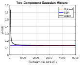
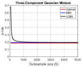
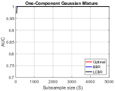
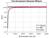
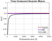
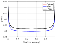
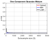
where cksubscript𝑐𝑘c_{k}’s are mixture weights. We consider the case where the covariance matrix is isotropic and controlled with a single scale parameter σ𝜎\sigma. We consider three cases where K=1,2,3𝐾123K=1,2,3 and σ=2,3,4𝜎234\sigma=2,3,4 where the increasing value of K𝐾K and σ𝜎\sigma makes the problem gradually more difficult. The mean values for class one are sampled from the unit cube in positive orthant and class zero from unit cube in negative orthant. The curves are obtained by averaging 50 experiments. For any given pair of conditional distributions the optimal ranking function minimizing the ϕitalic-ϕ\phi-risk is found by calculating μ𝜇\mathbf{\mu} and 𝚺𝚺\mathbf{\Sigma} and solving the ϕitalic-ϕ\phi-risk minimization problem. On the other hand, the optimal ranking function maximizing the AUC is the likelihood ratio of class-conditionals, which is a consequence of the Neyman-Pearson lemma [29]. Figure 1 shows the results of our experiments. For panels (a)-(f) we have ρ=0.5𝜌0.5\rho=0.5 with 103superscript10310^{3} positive and negative samples. So BBR uses 106superscript10610^{6} pairs whereas LCBR uses the number shown on the x-axis. In panels (a)-(c) we show the ϕitalic-ϕ\phi-risk and in (d)-(f) we show the AUC. As the number of components increase the problem becomes more difficult, resulting in higher ϕitalic-ϕ\phi-risk and lower AUC for optimal ranking functions. In all cases BBR is very close to the optimal ranker; but it has high sample cost. LCBR, on the other hand, catches on with S=3000𝑆3000S=3000 at most. This is also reflected in wall clock times; as shown in panels (g)-(i) LCBR is roughly 100 times faster than BBR when S=5000𝑆5000S=5000 subsamples are used. Finally we illustrate the performance of BBR and LCBR as a function of label skew ρ𝜌\rho. In the proof of Lemma 1, we saw that applying McDiarmid’s inequality gives the term ρ(1ρ)𝜌1𝜌\rho(1-\rho) in the exponent. This suggests, as ρ𝜌\rho goes to 00 or 111 the generalization performance should decrease. Panel (j) shows that this is indeed the case: here BBR uses 2000ρ2000𝜌2000\rho positive and 2000(1ρ)20001𝜌2000(1-\rho) negative samples, whereas LCBR uses 5,00050005,000 subsamples. The performance of BBR and LCBR are once again close; but as ρ𝜌\rho deviates from 0.50.50.5 the generalization of both algorithms get worse.

5.2 LIBSVM Datasets

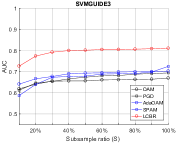
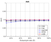
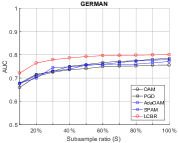
We now compare LCBR against state-of-the art algorithms on three datasets from LIBSVM. The algorithms we implement, in addition to LCBR, are the following: AdaOAM [8] uses adaptive stochastic gradient descent with pairwise squared loss, whereas PGD is SGD based approach [7]. SPAM is one of the most recent works where AUC optimization is formulated as a stochastic saddle point problem [19]. OAM is a relatively older algorithm, but we include it as it is based in a different objective, the pairwise hinge loss [4]. As widely done in the literature, we use AUC on test set as the performance measure. We use the train and test splits provided by LIBSVM. Regularization parameters are determined by cross-validation and step sizes are chosen based on the references. The experiments are averaged over 50 runs.

We show the results in Figure 2. The x-axis correspond to the number of subsamples used as a percentage of total number of samples available. For example, A9A dataset contains approximately 33K33𝐾33K data points. A subsample ratio of 50%percent5050\% implies we use approximately 16.5K16.5𝐾16.5K random samples from this dataset. For the A9A dataset all algorithms have good generalization, with an AUC of approximately 90%percent9090\%. For the GERMAN and SVMGUIDE3 datasets, on the other hand, there is a significant gap between LCBR and the SGD-based competitiors. Here the SGD and learning rate free approach of LCBR proves useful and it achieves better generalization for the given number of samples. Therefore the sample complexity of LCBR is favorable.

5.3 Algorithmic Complexity

For the algorithms presented in this paper, it can be seen that the computational bottleneck is at the accumulation phase (cf. Algorithms 1 and 2). For BBR the cost of this step is O(N1N0D2)𝑂subscript𝑁1subscript𝑁0superscript𝐷2O(N_{1}N_{0}D^{2}) and for LCBR this is O(SD2)𝑂𝑆superscript𝐷2O(SD^{2}). Typically SN1N0much-less-than𝑆subscript𝑁1subscript𝑁0S\ll N_{1}N_{0} which can save significant computation. On the other hand, the storage for both BBR and LCBR is O(D2)𝑂superscript𝐷2O(D^{2}) as it requires storing the covariance matrix. This quadratic dependence on dimension can be an issue when D𝐷D is too large. In this case, a sparse approximation of 𝚺Ssubscript𝚺𝑆\mathbf{\Sigma}_{S} can be necessary. However, note that this storage bottleneck is also present in the algorithms we compared [4, 7, 8]. In contrast, SPAM [19] can be implemented in O(D)𝑂𝐷O(D) space; however that algorithm requires knowledge of expectations with respect to the true conditionals, which is unknown in practice. Our experiments show that LCBR can still achieve better performance.
Refer to caption
(a)
Refer to caption
(b)
Refer to caption
(c)
Figure 2: Results of experiments with LIBSVM datasets.

6 Conclusion

We have considered the problem of bipartite ranking, where the empirical AUC loss is replaced with the pairwise squared loss. Different from the previous work—which was based on SGD—we proposed a low sample cost bipartite ranking algorithm (LCBR), and showed that the number of samples required for good performance obeys SN1N0much-less-than𝑆subscript𝑁1subscript𝑁0S\ll N_{1}N_{0}. Experiments show that LCBR quickly achieves similar performance with BBR where the number of samples are several order of magnitudes lower. Experiments against state-of-the-art bipartite ranking algorithms also show that LCBR can achieve better generalization with a smaller subsample set. In a longer version of the paper we will also consider extending these results to random feature spaces, which include random kernel features and random neural networks.

7 Appendix: Proof of Lemma 2

For the proofs we will use the shorthand 𝐱s=𝐱is1𝐱js0subscript𝐱𝑠superscriptsubscript𝐱subscript𝑖𝑠1superscriptsubscript𝐱subscript𝑗𝑠0\mathbf{x}_{s}=\mathbf{x}_{i_{s}}^{1}-\mathbf{x}_{j_{s}}^{0}.

(i) We recall the Matrix Bernsten Inequality for a D×D𝐷𝐷D\times D symmetric, random matrix 𝐙𝐙\mathbf{Z} and threshold γ𝛾\gamma:

P(𝐙2>γ)2Dexp(γ2/2𝕍(𝐙)+Lγ/3)𝑃subscriptnorm𝐙2𝛾2𝐷superscript𝛾22𝕍𝐙𝐿𝛾3\displaystyle P(\left\|\mathbf{Z}\right\|_{2}>\gamma)\leq 2D\exp\left(-\frac{\gamma^{2}/2}{\mathbb{V}(\mathbf{Z})+L\gamma/3}\right) (25)

where L𝐿L is a norm bound on summands.

First apply a spectral norm bound to the quadratic expression: sup𝐰1𝒲|Δ𝚺|W2𝚺S𝚺N2subscriptsupremumsubscript𝐰1𝒲subscriptΔ𝚺superscriptsubscript𝑊2subscriptnormsubscript𝚺𝑆subscript𝚺𝑁2\sup_{\mathbf{w}_{1}\in\mathcal{W}}\left|\Delta_{\mathbf{\Sigma}}\right|\leq W_{*}^{2}\left\|\mathbf{\Sigma}_{S}-\mathbf{\Sigma}_{N}\right\|_{2}. We now take 𝐙=𝚺S𝚺N𝐙subscript𝚺𝑆subscript𝚺𝑁\mathbf{Z}=\mathbf{\Sigma}_{S}-\mathbf{\Sigma}_{N}. The spectral norm can be bounded based on the argument in [30]. We can decompose 𝐙𝐙\mathbf{Z} into a sum: 𝐙=s=1S(1/S)[𝐱s𝐱s𝚺N]𝐙superscriptsubscript𝑠1𝑆1𝑆delimited-[]subscript𝐱𝑠superscriptsubscript𝐱𝑠topsubscript𝚺𝑁\mathbf{Z}=\sum_{s=1}^{S}(1/S)[\mathbf{x}_{s}\mathbf{x}_{s}^{\top}-\mathbf{\Sigma}_{N}]. We denote each summand by 𝐄s=(1/S)[𝐱s𝐱s𝚺N]subscript𝐄𝑠1𝑆delimited-[]subscript𝐱𝑠superscriptsubscript𝐱𝑠topsubscript𝚺𝑁\mathbf{E}_{s}=(1/S)[\mathbf{x}_{s}\mathbf{x}_{s}^{\top}-\mathbf{\Sigma}_{N}]. It then follows from triangle inequality that

𝐄s21S[𝐱s𝐱s2+𝚺N2]2S𝐱s228X2Ssubscriptnormsubscript𝐄𝑠21𝑆delimited-[]subscriptnormsubscript𝐱𝑠superscriptsubscript𝐱𝑠top2subscriptnormsubscript𝚺𝑁22𝑆superscriptsubscriptnormsubscript𝐱𝑠228superscriptsubscript𝑋2𝑆\displaystyle\left\|\mathbf{E}_{s}\right\|_{2}\leq\frac{1}{S}\left[\left\|\mathbf{x}_{s}\mathbf{x}_{s}^{\top}\right\|_{2}+\left\|\mathbf{\Sigma}_{N}\right\|_{2}\right]\leq\frac{2}{S}\left\|\mathbf{x}_{s}\right\|_{2}^{2}\leq\frac{8X_{*}^{2}}{S} (26)

where the second inequality follows from Jensen’s inequality. Since the subsampling is conditional on 𝒩𝒩\mathcal{N}, 𝚺Nsubscript𝚺𝑁\mathbf{\Sigma}_{N} is constant with respect to the subsampled pairs, and each summand is centered and i.i.d. The variance of the sum decomposes as 𝕍(𝐙)=sS𝔼[𝐄s2]2𝕍𝐙subscriptnormsubscript𝑠𝑆𝔼delimited-[]superscriptsubscript𝐄𝑠22\mathbb{V}(\mathbf{Z})=\left\|\sum_{s\in S}\mathbb{E}[\mathbf{E}_{s}^{2}]\right\|_{2}. For a single summand the second moment can be bounded as

𝔼[𝐄s2]=1S2𝔼[[𝐱s𝐱s𝚺N]2]=1S2[𝔼[𝐱s22𝐱s𝐱s]𝚺N2]4X2S2𝚺N𝔼delimited-[]superscriptsubscript𝐄𝑠21superscript𝑆2𝔼delimited-[]superscriptdelimited-[]subscript𝐱𝑠superscriptsubscript𝐱𝑠topsubscript𝚺𝑁21superscript𝑆2delimited-[]𝔼delimited-[]superscriptsubscriptnormsubscript𝐱𝑠22subscript𝐱𝑠superscriptsubscript𝐱𝑠topsuperscriptsubscript𝚺𝑁2precedes-or-equals4superscriptsubscript𝑋2superscript𝑆2subscript𝚺𝑁\displaystyle\mathbb{E}[\mathbf{E}_{s}^{2}]=\frac{1}{S^{2}}\mathbb{E}\left[\left[\mathbf{x}_{s}\mathbf{x}_{s}^{\top}-\mathbf{\Sigma}_{N}\right]^{2}\right]=\frac{1}{S^{2}}\left[\mathbb{E}\left[\left\|\mathbf{x}_{s}\right\|_{2}^{2}\mathbf{x}_{s}\mathbf{x}_{s}^{\top}\right]-\mathbf{\Sigma}_{N}^{2}\right]\preceq\frac{4X_{*}^{2}}{S^{2}}\mathbf{\Sigma}_{N} (27)

from which the variance inequality 𝕍(𝐙)(4X2/S)𝚺N2𝕍𝐙4superscriptsubscript𝑋2𝑆subscriptnormsubscript𝚺𝑁2\mathbb{V}(\mathbf{Z})\leq(4X_{*}^{2}/S)\left\|\mathbf{\Sigma}_{N}\right\|_{2} follows. Substituting these to Eq. (25) with γ=ϵ/W2𝛾italic-ϵsuperscriptsubscript𝑊2\gamma=\epsilon/W_{*}^{2} yields the result.

(ii) We recall the following concentration inequality for i.i.d. and bounded random vectors with mean 𝐱¯¯𝐱\bar{\mathbf{x}} [12]:

P(1Ss=1S𝐱s𝐱¯2γ)exp{12(γSL1)2}.𝑃subscriptnorm1𝑆superscriptsubscript𝑠1𝑆subscript𝐱𝑠¯𝐱2𝛾12superscript𝛾𝑆𝐿12\displaystyle P\left(\left\|\frac{1}{S}\sum_{s=1}^{S}\mathbf{x}_{s}-\bar{\mathbf{x}}\right\|_{2}\geq\gamma\right)\leq\exp\left\{-\frac{1}{2}\left(\frac{\gamma\sqrt{S}}{L}-1\right)^{2}\right\}~{}. (28)

From the following inequalities

sup𝐰1,𝐰2𝒲|Δσ(𝐰1,𝐰2)|sup𝐰1,𝐰2𝐰1𝐰2SμNμS22W1Ss=1S𝐱sμN2subscriptsupremumsubscript𝐰1subscript𝐰2𝒲subscriptΔ𝜎subscript𝐰1subscript𝐰2subscriptsupremumsubscript𝐰1subscript𝐰2subscriptnormsubscript𝐰1subscript𝐰2𝑆subscriptnormsubscript𝜇𝑁subscript𝜇𝑆22subscript𝑊subscriptnorm1𝑆superscriptsubscript𝑠1𝑆subscript𝐱𝑠subscript𝜇𝑁2\displaystyle\sup_{\mathbf{w}_{1},\mathbf{w}_{2}\in\mathcal{W}}\left|\Delta_{\sigma}(\mathbf{w}_{1},\mathbf{w}_{2})\right|\leq\sup_{\mathbf{w}_{1},\mathbf{w}_{2}}\left\|\mathbf{w}_{1}-\mathbf{w}_{2}\right\|_{S}\left\|\mathbf{\mu}_{N}-\mathbf{\mu}_{S}\right\|_{2}\leq 2W_{*}\left\|\frac{1}{S}\sum_{s=1}^{S}\mathbf{x}_{s}-\mathbf{\mu}_{N}\right\|_{2} (29)

the desired result is obtained by setting γ=ϵ/2W𝛾italic-ϵ2subscript𝑊\gamma=\epsilon/2W_{*} and L=X𝐿subscript𝑋L=X_{*} in Eq. (28). \hfill\square

References

  • [1] H. B. McMahan, G. Holt, D. Sculley, M. Young, D. Ebner, J. Grady, L. Nie, T. Phillips, E. Davydov, D. Golovin, S. Chikkerur, D. Liu, M. Wattenberg, A. M. Hrafnkelsson, T. Boulos, and J. Kubica, “Ad click prediction: a view from the trenches,” in Conference on Knowledge Discovery and Data Mining, 2013.
  • [2] J. Hu, H. Yang, M. Lyu, I. King, and A. So, “Online Nonlinear AUC Maximization for Imbalanced Data Sets,” IEEE Transactions on Neural Networks and Learning Systems, 2016.
  • [3] X. Hong, S. Chen, and C. J. Harris, “A Kernel-Based Two-Class Classifier for Imbalanced Data Sets,” IEEE Transactions on Neural Networks, 2007.
  • [4] P. Zhao, S. C. H. Hoi, R. Jin, and T. Yang, “Online AUC Maximization,” in International Conference on Machine Learning, 2011.
  • [5] W. Gao, R. Jin, S. Zhu, and Z.-H. Zhou, “One-Pass AUC Optimization,” in International Conference on Machine Learning, 2013.
  • [6] W. Gao and Z.-H. Zhou, “On the Consistency of AUC Pairwise Optimization,” in International Joint Conference on Artificial Intelligence, 2015.
  • [7] M. Boissier, S. Lyu, Y. Ying, and D.-X. Zhou, “Fast Convergence of Online Pairwise Learning Algorithms,” in International Conference on Artificial Intelligence and Statistics, 2016.
  • [8] Y. Ding, P. Zhao, S. C. H. Hoi, and Y. S. Ong, “An Adaptive Gradient Method for Online AUC Maximization,” in Association for Advancement of Artificial Intelligence, 2015.
  • [9] P. Kar, B. Sriperumbudur, P. Jain, and H. Karnick, “On the Generalization Ability of Online Learning Algorithms for Pairwise Loss Functions,” in International Conference on Machine Learning, 2013.
  • [10] M. Mohri, A. Rostamizadeh, and A. Talwalkar, Foundations of Machine Learning.   MIT Press, 2012.
  • [11] S. Agarwal, T. Graepel, R. Herbrich, S. Har-Peled, and D. Roth, “Generalization Bounds for the Area Under the ROC Curve,” Journal of Machine Learning Research, 2005.
  • [12] A. Rahimi and B. Recht, “Weighted sums of random kitchen sinks: Replacing minimization with randomization in learning,” in Advances in Neural Information Processing Systems, 2008.
  • [13] Y. Wang, R. Khardon, D. Pechyony, and R. Jones, “Generalization Bounds for Online Learning Algorithms with Pairwise Loss Functions,” in Conference on Learning Theory, 2012.
  • [14] S. Clemencon, G. Lugosi, and N. Vayatis, “Ranking and empirical minimization of U-Statistics,” The Annals of Statistics, 2008.
  • [15] T. Peel, A. Sandrine, and L. Ralaivola, “Empirical Bernstein Inequalities for U-Statistics,” in Advances in Neural Information Processing Systems, 2010.
  • [16] Y. Lei, S.-B. Lin, and K. Tang, “Generalization Bounds for Regularized Pairwise Learning,” in International Joint Conference on Artificial Intelligence, 2018.
  • [17] S. Agarwal and P. Niyogi, “Generalization Bounds for Ranking Algorithms via Algorithmic Stability,” Journal of Machine Learning Research, 2009.
  • [18] C. Cortes, M. Mohri, and A. Rastogi, “Magnitude-Preserving Ranking Algorithms,” in International Conference on Machine Learning, 2007.
  • [19] M. Natole Jr., Y. Ying, and S. Lyu, “Stochastic Proximal Algorithms for AUC Maximization,” in International Conference on Machine Learning, 2018.
  • [20] Y. Ying, L. Wen, and S. Lyu, “Stochastic Online AUC Maximization,” in Advances in Neural Information Processing Systems, 2016.
  • [21] P. L. Bartlett, M. I. Jordan, and J. D. McAuliffe, “Convexity, classification, and risk bounds,” Journal of the American Statistical Association, 2006.
  • [22] S. Agarwal, “Surrogate Regret Bounds for Bipartite Ranking via Strongly Proper Losses,” Journal of Machine Learning Research, 2014.
  • [23] W. Kotlowski, K. J. Dembczynski, and E. Huellermeier, “Bipartite ranking through minimization of univariate loss,” in International Conference on Machine Learning, 2011.
  • [24] Y. Ding, C. Liu, P. Zhao, and S. C. Hoi, “Large Scale Kernel Methods for Online AUC Maximization,” in International Conference on Data Mining (ICDM), 2017.
  • [25] J. Hu, H. Yang, M. Lyu, I. King, and A. So, “Kernelized Online Imbalanced Learning with Fixed Budgets,” in Association for Advancement of Artificial Intelligence (AAAI), 2015.
  • [26] H. Narasimhan and S. Agarwal, “On the Relationship Between Binary Classification, Bipartite Ranking, and Binary Class Probability Estimation,” in Advances in Neural Information Processing Systems, 2013.
  • [27] S. Agarwal, “Generalization bounds for some ordinal regression algorithms,” in Proceedings of the 19th International Conference on Algorithmic Learning Theory, 2008.
  • [28] A. Rajkumar and S. Agarwal, “When Can We Rank Well from Comparisons of O(n log n) Non-Actively Chosen Pairs?” in Conference on Learning Theory, 2016.
  • [29] H. V. Poor, An Introduction to Signal Detection and Estimation.   Springer, 1998.
  • [30] J. Tropp, “An introduction to matrix concentration inequalities,” Foundations and Trends in Machine Learning, 2015.