The intriguing role of module criticality in the generalization of deep networks

Abstract

We study the phenomenon that some modules of deep neural networks (DNNs) are more critical than others. Meaning that rewinding their parameter values back to initialization, while keeping other modules fixed at the trained parameters, results in a large drop in the network’s performance. Our analysis reveals interesting properties of the loss landscape which leads us to propose a complexity measure, called module criticality, based on the shape of the valleys that connect the initial and final values of the module parameters. We formulate how generalization relates to the module criticality, and show that this measure is able to explain the superior generalization performance of some architectures over others, whereas, earlier measures fail to do so.

1 Introduction

Neural networks have had tremendous practical impact in various domains such as revolutionizing many tasks in computer vision, speech and natural language processing. However, many aspects of their design and analysis have remained mysterious to this date. One of the most important questions is “what makes an architecture work better than others given a specific task?” Extensive research in this area has led to many potential explanations on why some types of architectures have better performance; however, we lack a unified view that provides a complete and satisfactory answer. In order to attain a unified view on superiority of one architecture over another in terms of generalization performance, we need to come up with a measure that effectively captures this.

(a)

(b)

Figure 1: Module Criticality: Loss values in the valleys that connect the initial weights $\theta^{0}$ to the final weights $\theta^{F}$ of a non-critical (left) and a critical (right) module in the ResNet18 architecture. Given a ball with radius $r$ (length of the red line), module criticality can be defined as how far one can push the ball in the valley towards initialization (length of the white dashed line) divided by the radius $r$. Hence, non-critical modules are the ones with a wide valley connecting the initial weight vector to the final one whereas in critical modules, the valley either becomes too sharp or the loss values start to increase when the ball comes too close to the initial weight. The $x$ axis is simply chosen to be parallel to $\theta^{F}-\theta^{0}$ and the $y$ axis is a compact representation of all other dimensions generated by adding Gaussian noise to the the points on the convex combination of $\theta^{0}$ and $\theta^{F}$ and evaluating the loss. The sign on the $y$ axis is decided based on the sign of the inner product of the noise to $\theta^{0}$.

Analyzing the generalization behavior of neural networks has been an active area of research since Baum and Haussler (1989). Many generalization bounds and complexity measures have been proposed so far.  Bartlett (1998) emphasized the importance of the norm of the weights in predicting the generalization error. Since then various analysis have been proposed. These results are either based on covering number and Rademacher complexity (Neyshabur et al., 2015; Bartlett et al., 2017; Neyshabur et al., 2019; Long and Sedghi, 2019; Wei and Ma, 2019), or they use approaches similar to PAC-Bayes (McAllester, 1999; Dziugaite and Roy, 2017; Neyshabur et al., 2017; Neyshabur et al., 2018; Arora et al., 2018; Nagarajan and Kolter, 2019a; Zhou et al., 2019). Recently authors have emphasized on the role of distance to initialization rather than norm of the weights in generalization (Dziugaite and Roy, 2017; Nagarajan and Kolter, 2019b; Neyshabur et al., 2019; Long and Sedghi, 2019). Earlier results have an exponential dependency on the depth and focus on fully connected networks. More recently, Long and Sedghi (2019) provided generalization bounds for convolutional neural networks (CNNs) and fully connected networks used in practice and their bounds have linear dependency on the depth.

Despite the success of earlier works in capturing the dependency of generalization performance of a model on different parameters, they fail at the following task: Rank the generalization performance of candidate architectures for a specific task such that the ranking aligns well with the ground truth. Moreover, majority of these bounds are proposed for fully connected modules and it is not straightforward to evaluate them for different architectures such as ResNets.

Every DNN architecture is a computation graph where each node is a module. We are interested in understanding how different modules in the network interact with each other and influence generalization performance as a whole. To do so, we delve deeper into the phenomenon of “module criticality” which was reported by Zhang et al. (2019). They observed that modules of the network present different robustness characteristics to parameter perturbation. Specifically, they look into the following perturbation: Rewind one module back to its initialization value while keeping all other modules fixed (at the final trained value). They note that the impact of this perturbation on network performance varies between modules and depends on which module was rewound. Some modules are “critical” meaning that rewinding their value to the initialization harms the network performance, while for others the impact of this perturbation on performance is negligible. They show that various conventional DNN architectures exhibit this phenomenon.

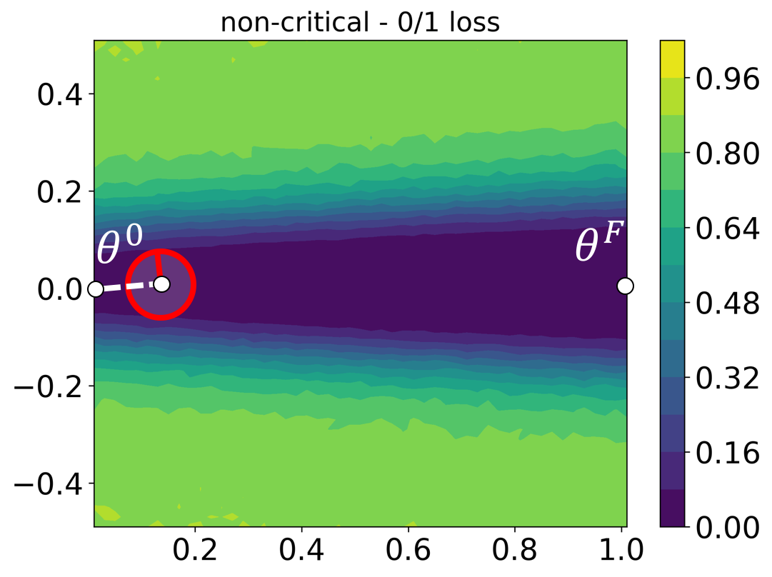
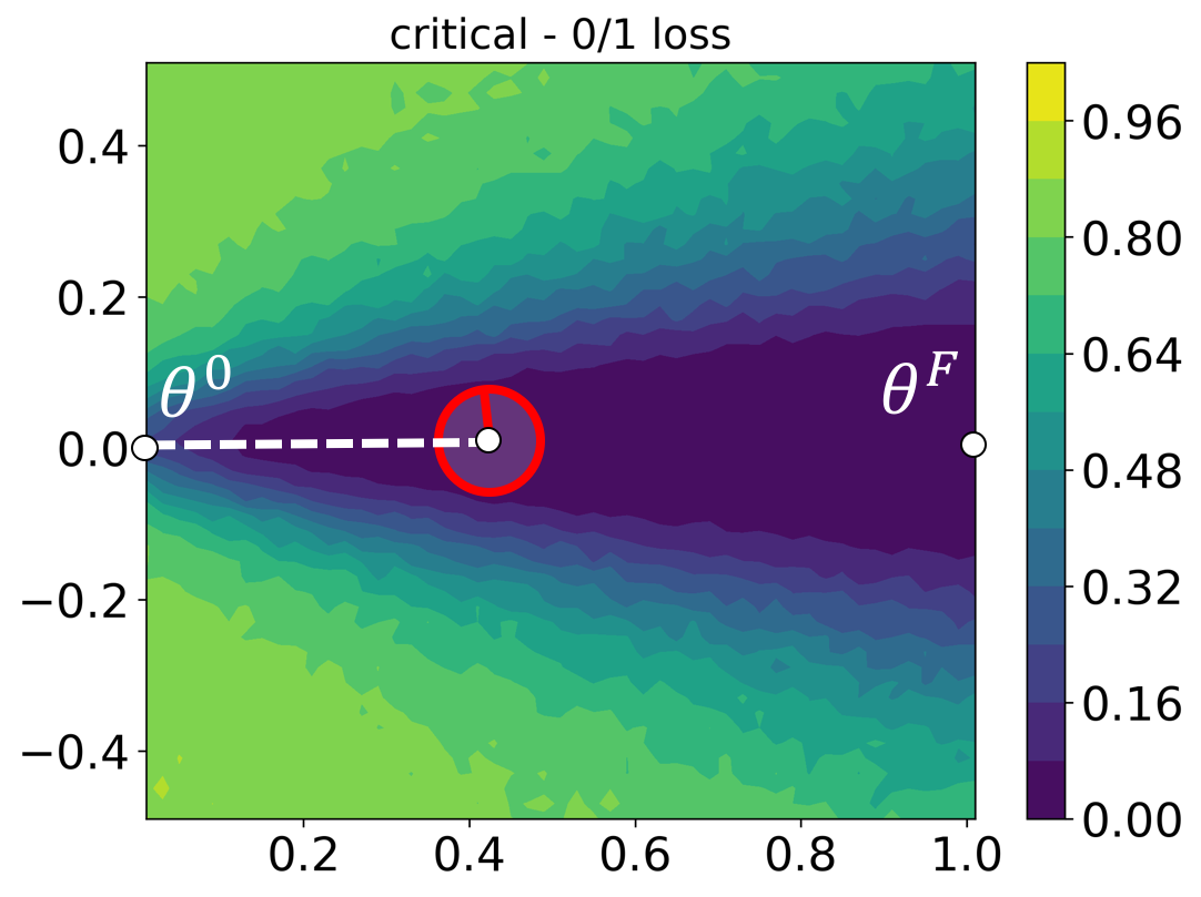
Let us now informally define what we mean by the measure “module criticality” (see Figure 1). For each module, we move on a line from its final trained value to its initialization value (convex combination path) while keeping all other modules fixed at their trained value. Then we measure the performance drop. Let $\theta^{\alpha}_{i}=(1-\alpha)\theta_{i}^{0}+\alpha\theta_{i}^{F},\alpha\in[0,1]$ be the convex combination between initial weights $\theta^{0}_{i}$ and the final weights $\theta^{F}_{i}$ at module $i$, where $\alpha_{i}$ is the minimum value between $0$ and $1$ when performance (train error) of the network drops by at most a threshold value ${\epsilon}$. If $\alpha_{i}$ is small we can move a long way back to initialization without hurting performance and the “module criticality” of this module would be low. Further, we also wish to incorporate the robustness to noise (that is, the valley width) for the module along this path. If the module is robust to noise along this path (that is, the valley is wide) then the module criticality would again be low (see Definition 3.1 for a formal definition).

In this paper, we seek to study this phenomenon in depth and shed some light on it by showing that conventional complexity measures cannot capture criticality (see Section 2). Next, we theoretically formulate this phenomenon and analyze its role in generalization. Through this analysis, we provide a new generalization measure that captures the dissimilarity of different modules and depicts how it influences the generalization of the corresponding DNN. Intuitively, the closer we can get to initialization for each module, the better the generalization.

We analyze the relation between generalization and module criticality through a PAC-Bayesian analysis. In Section 3 we show that it is the overall network criticality measure and not the number of critical modules that controls generalization. If the network criticality measure is smaller for an architecture, it has better generalization performance. In Section 4, we demonstrate through various experiments that our proposed measure is able to distinguish between different network architectures in terms of their generalization performance. Moreover, the network criticality measure is able to correctly rank the generalization performance of different architectures better than the measures proposed earlier.

Notation:

We use upper case letters for matrices. The operator norm and Frobenius norm of $M$ are denoted by $\lVert M\rVert_{2}$, $\lVert M\rVert_{\text{Fr}}$ respectively. For $n\in\mathbb{N}$, we use $[n]$ to denote the set $\{1,\dotsc,n\}$. Let $\mathcal{L}_{S}(f)$ be the loss of function $f$ on the training set $S$ with $m$ samples. We are mainly interested in the classification task where $\mathcal{L}_{S}(f)=\frac{1}{m}\sum_{(x,y)\in S}\mathbf{1}[f(x)[y]\leq\max_{j\neq y}f(x)[j]]$. For any $\gamma>0$, we also define margin loss $\mathcal{L}_{S,\gamma}(f)=\frac{1}{m}\sum_{(x,y)\in S}\mathbf{1}[f(x)[y]\leq\gamma+\max_{j\neq y}f(x)[j]]$. Let $\mathcal{L}_{D}(f)$ be the loss of function $f$ on population data distribution $D$ defined similar to $\mathcal{L}_{S}(f)$. We will denote the function parameterized by $\Theta$ by $f_{\Theta}$.

2 Towards understanding module criticality

2.1 Setting

A DNN architecture is a directed acyclic computation graph which may or may not be layered. In order to have a unifying definition between different architectures, we use the notion of a “module”. A module is a node in the computation graph that has incoming edges from other modules and outgoing edges to other nodes, and performs a linear transformation on its inputs. For a layered model such as a VGG, a module is equivalent to a layer. On the other hand, in a ResNet some modules are parallel to each other. For example, a downsample module and the concatenation of two convolutional modules in a ResNet18-v1 architecture. Note that, similar to conventional definitions the non-linearity (such as a ReLU) is not part of the module.

Figure 2: Analysis of rewinding modules to initialization for the ResNet-18 architecture. Each row represents a module in ResNet18-v1 and each column represents a particular training epoch to which this module is rewound to. The difference from analysis of Zhang et al. (2019) is that we rewind each module, whereas Zhang et al. (2019) rewind the entire ResNet blocks.

Let $\Theta=(\theta_{1},\dotsc,\theta_{d})$ correspond to all parameters of a DNN with $d$ modules, where $\theta_{i}$ refers to the weight matrix (or operator matrix in case of convolution) at module $i$ and $\theta_{i}^{0},\theta_{i}^{F}$ refer to the value of weight matrix at initialization and the end of training, respectively. For sequential architectures, $d$ is equal to the depth of the network but that is not necessarily true for a general architectures such as a ResNet.

2.2 Robustness to rewinding

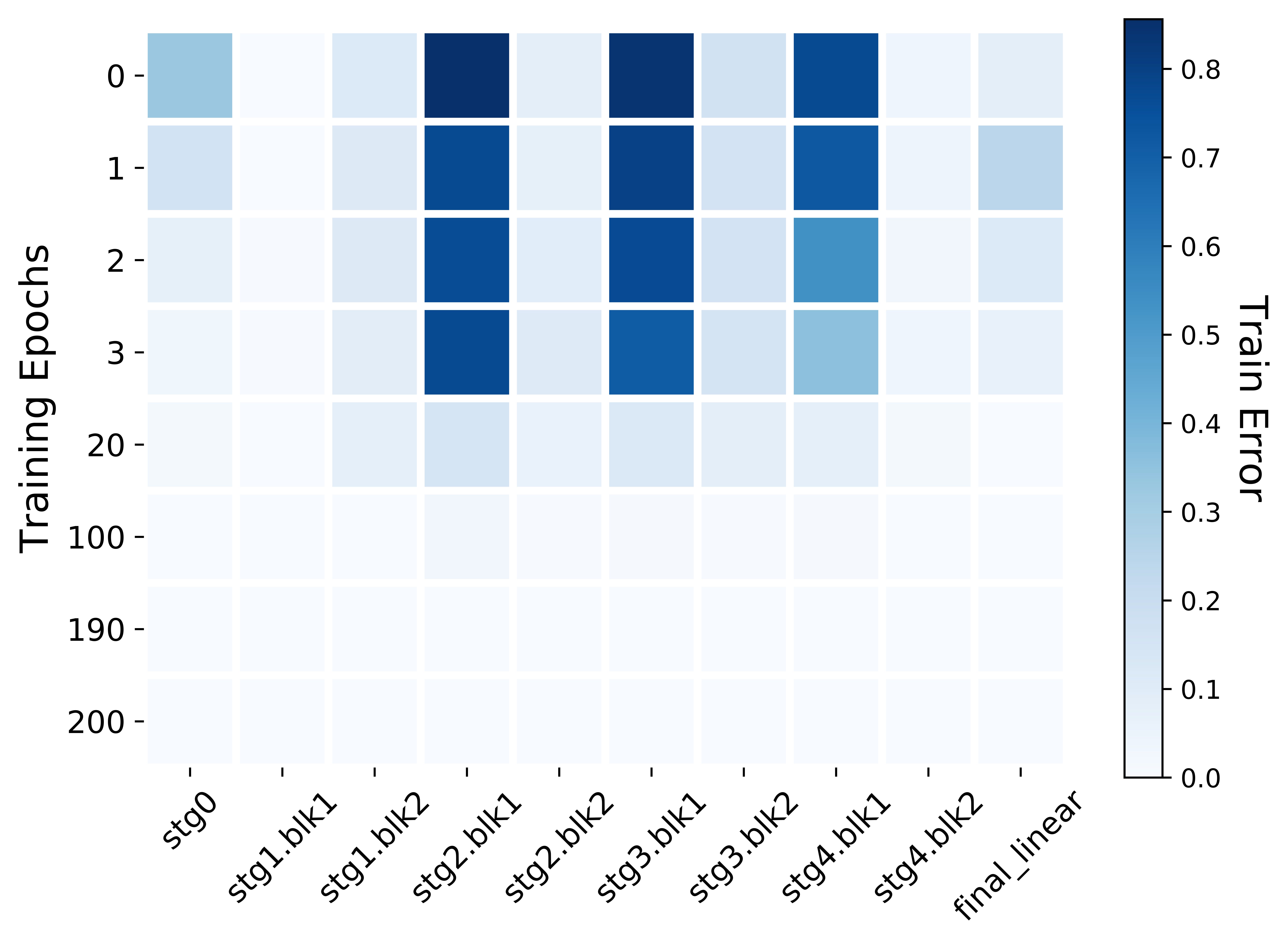
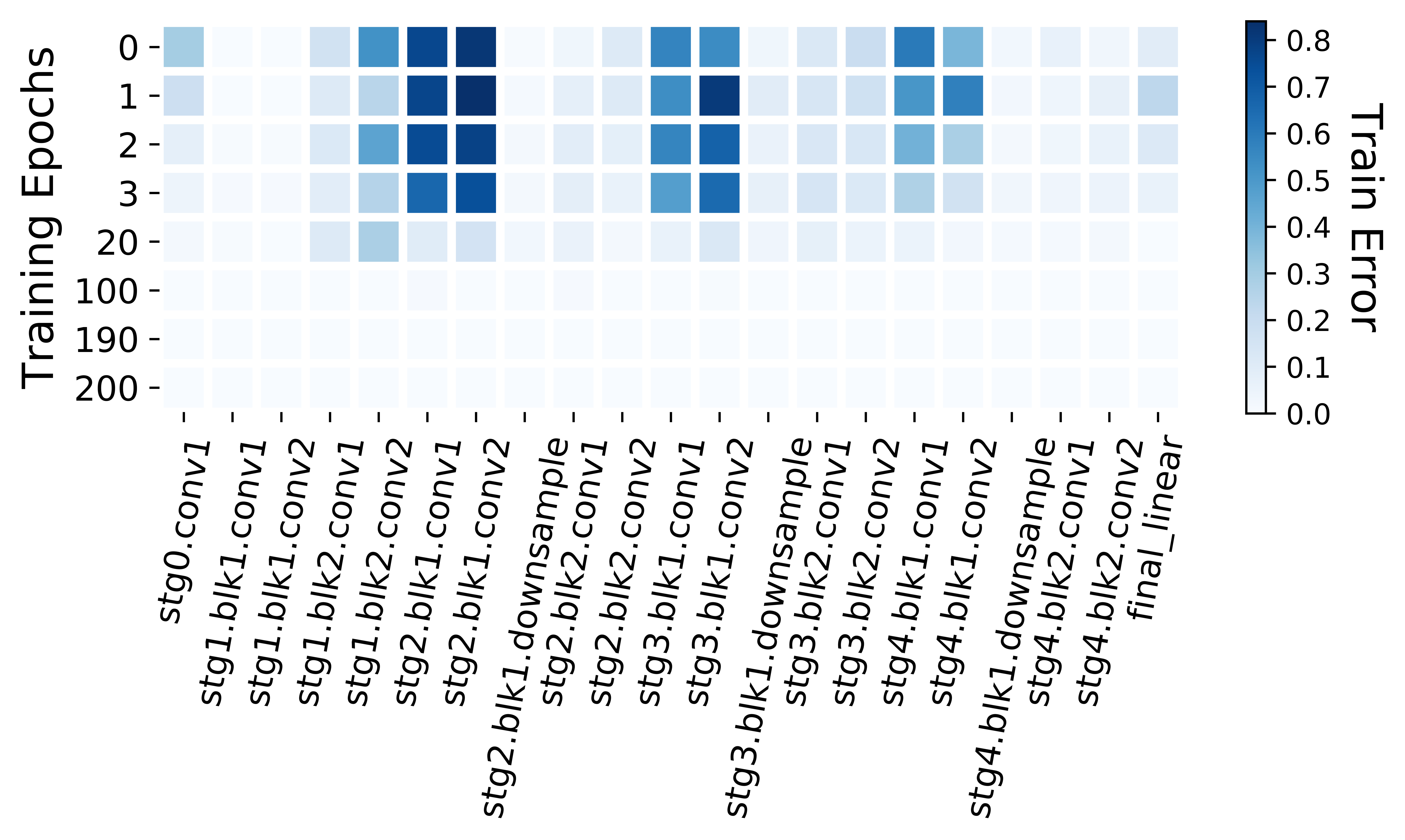
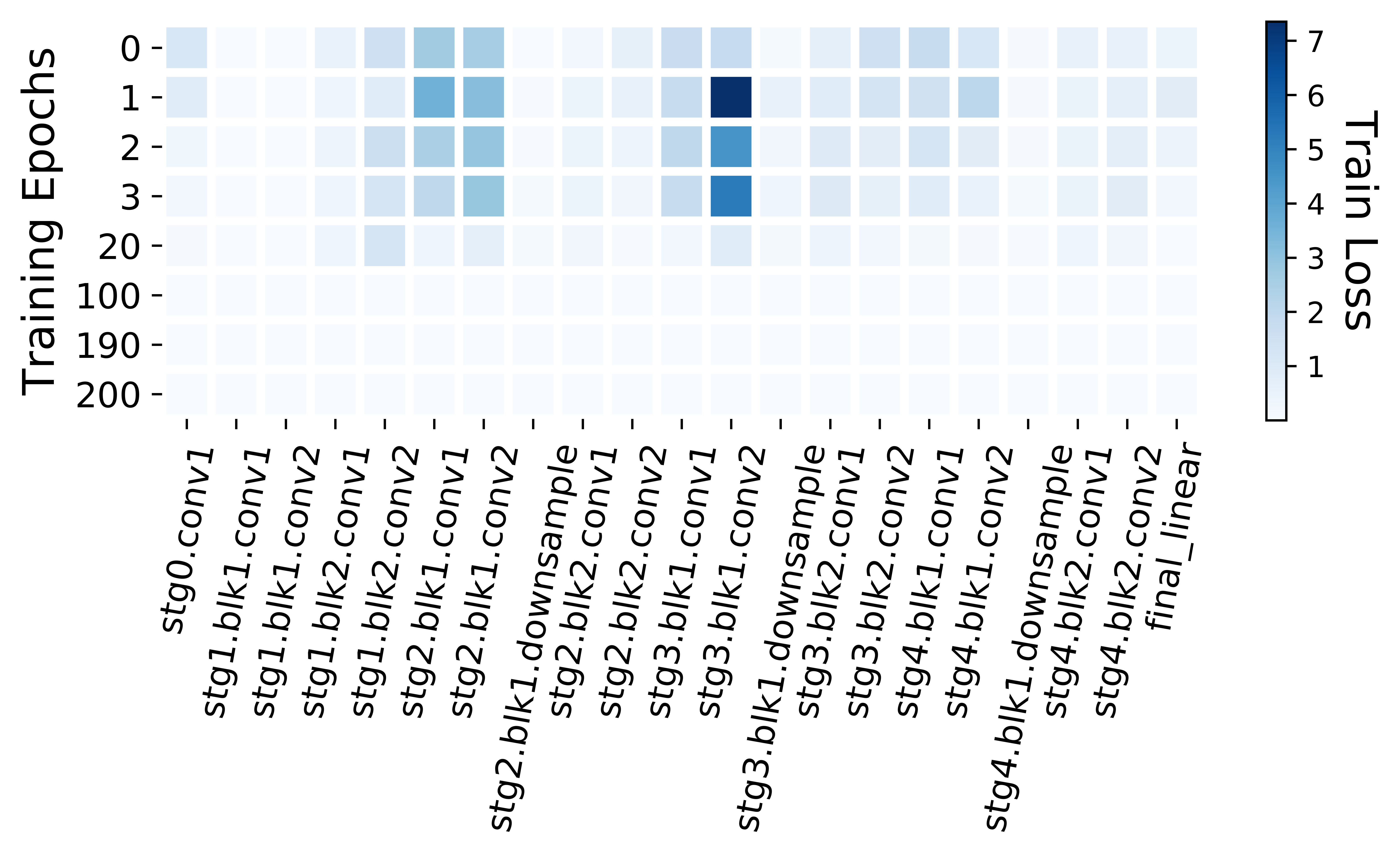
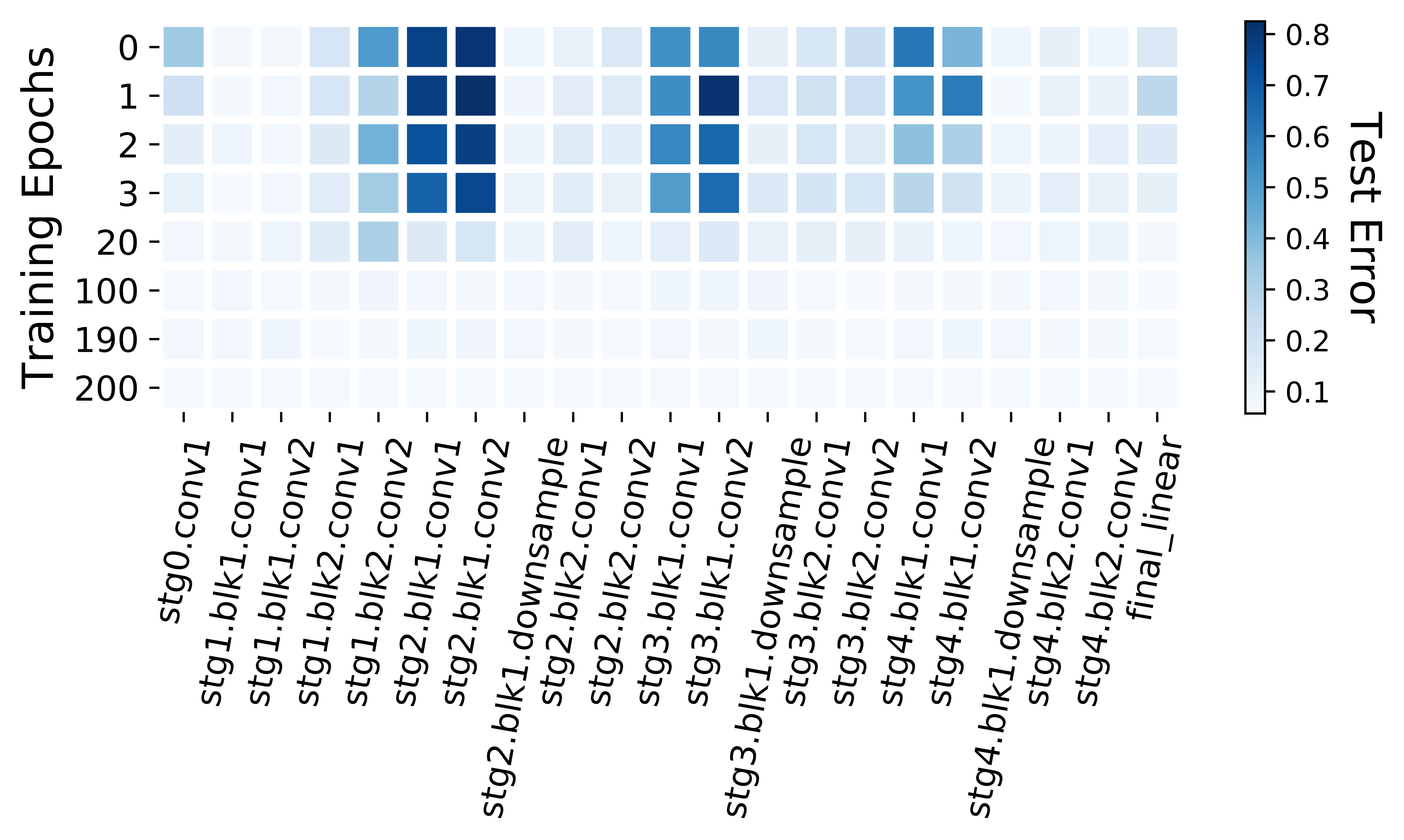
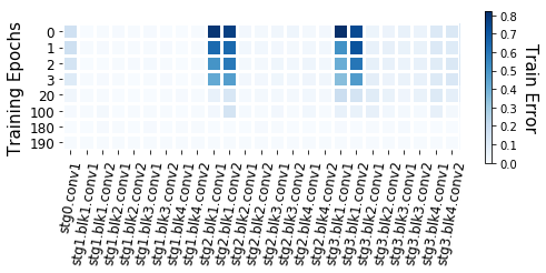
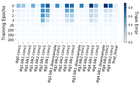
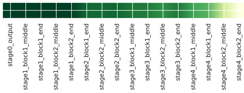
Consider the following perturbation to a trained network at some training epoch as considered by Zhang et al. (2019). For each module in the network, rewind its value back to its value at this training epoch while keeping the values of all other modules fixed (at their final trained value). Next, measure the change in performance of the model before and after this manipulation. We repeat a similar analysis that differs from that of Zhang et al. (2019) in one detail. Zhang et al. (2019) rewind the whole ResNet block at once, whereas, we rewind each module (each convolutional module) separately. This rewind analysis is shown in Figure 2 for ResNet18-v1. Each column represents a module in ResNet18-v1 and each row represents a particular training epoch to which this module is rewound to. Similar to earlier analysis, we observe that for many modules of the network, this manipulation does not influence the network performance drastically, while, for some others the impact is more pronounced. For example, in Figure 2 we look at the effect of rewinding on train error. The “Stage2.block1.conv2” module is critical, whereas, most other modules, once rewound, do not affect the performance. In Figure 6 in Appendix E we plot the effect of rewinding on different performance criteria (train loss, train error and test error) and observe that they exhibit a similar trend.

A stable phenomena:

The plots in Figure 2 capture a network trained with SGD with weights initialized using the standard Kaiming initialization (He et al., 2015). To ensure that the observed phenomenon is not an artifact of the training method and the initialization scheme, we repeated the experiments with different initialization and optimization methods. We saw a similar pattern. For example, Figures 7a, 7b in the appendix illustrate the pattern when we changed the initialization to Fixup (Zhang et al., 2019), and when we replace SGD with Adam (Kingma and Ba, 2014) respectively.

2.3 What measures fail to distinguish critical layers

(a) A non-critical module

(b) A critical module

Figure 3: Spectrum of a non-critical and a critical module during different epochs of training.

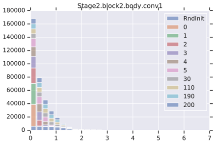
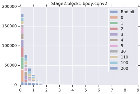
Spectrum of weight matrices:

We explore the change in the spectrum of different weight matrices on rewinding and note that the spectrum for a critical and non-critical module look similar. This is shown in Figure 3. We calculate the spectrum of convolutional layers using the algorithm by Sedghi et al. (2019).

Distance to initialization:

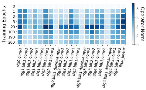
Next, we analyze the operator norm of difference from initialization for each module. Figure 8 in the appendix depicts this and reveals no difference between critical and non-critical modules. A similar plot was explored by Zhang et al. (2019), where they find that the Frobenius norm and the infinity norm also fail to capture criticality.

Change in the activation patterns:

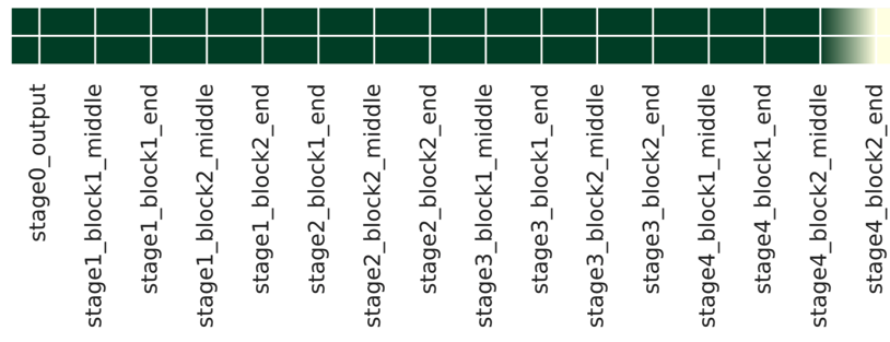
We investigated the change in the activation patterns of a network when we rewind a module. To do this, we study the similarity between two networks: 1. The original trained network and 2. The network with a rewound module. We use CKA (Kornblith et al., 2019) as the measure of similarity. For a non-critical module, the original and rewound networks are similar and in case of a critical module, the similarity between the activation patterns between the two networks degrades gradually rather than abruptly. See Figure 9 in Appendix E.

3 Generalization bounds based on module criticality

Our goal is to understand criticality and how it affects the generalization performance of a DNN. Inspired by the rewind to initialization experiments of Zhang et al. (2019), we take one step further and consider changing the value of each module, to the convex combination of its initial and final value. That is, for each module $i$, we replace $\theta_{i}$ with $\theta^{\alpha}_{i}=(1-\alpha)\theta_{i}^{0}+\alpha\theta_{i}^{F},\alpha\in[0,1],$ and keep all other layers fixed. Then we look at the effect of this perturbation on the performance of the network.

Figure 4 depicts how the train error, test error and train loss change as we decrease the value of $\alpha$ in $\theta^{\alpha}_{i}$ when $i$ refers to a critical module (yellow dashdot curve), a non-critical module (red dashed curve) and all modules (blue solid curve). We find that along this convex combination path all these performance measures degrade monotonically (increase in error and loss), as we move from the final weights to the initial weights.

The above experiment shows the effect of moving along a convex combination between module’s initial and trained value. To capture the relation between criticality and generalization, we are interested in also accounting for the width of the valley as we move from the final value to the initial value. In particular, we are interested in analyzing what happens if we are moving inside a ball of some radius $\sigma_{i}$ around each point in this path. PAC-Bayesian analysis, looks for a ball around final value of parameters such that the loss does not change if we move in this ball. Bringing this idea together with the one mentioned above, we are interested in moving from the final value to the initial value in a valley of some radius, and want to find out how far we can move on this path. Intuitively, being able to move closer to initialization values indicate that the effective function class is smaller and hence the network should generalize better. For example, in the extreme case where none of the weights change from their initialization value the function class would be a single function (the initial function) and the generalization error would be very low ($\sim$0$\%$) as both the train and test error would be very high (but equal). In this paper, we consider the case of trained models where train error is very low and hence low generalization error means good performance on test data.

Definition 3.1 (Module and Network Criticality).

Given an ${\epsilon}>0$ and network $f_{\Theta}$, we define the module criticality for module $i$ as follows:

$$\mu_{i,{\epsilon}}(f_{\Theta})=\min_{0\leq\alpha_{i},\sigma_{i}\leq 1}\left\{\frac{\alpha_{i}^{2}\left\|\theta_{i}^{F}-\theta_{i}^{0}\right\|_{\text{\emph{Fr}}}^{2}}{\sigma_{i}^{2}}:\mathbb{E}_{u\sim\mathcal{N}(0,\sigma_{i}^{2})}[\mathcal{L}_{S}(f_{\theta^{\alpha}_{i}+u,\Theta^{F}_{-i}})]\leq{\epsilon}\right\},$$ (1)

We also define the network criticality as the sum of the module criticality over modules of the network:

$$\mu_{\epsilon}(f_{\Theta})=\sum_{i=1}^{d}\mu_{i,{\epsilon}}(f_{\Theta}).$$ (2)

Here, $\mathcal{L}_{S}$ denotes the empirical zero-one loss over the training set, $f_{\theta^{\alpha}_{i},\Theta^{F}_{-i}}$ is the DNN’s function value where weight matrix corresponding to $i^{th}$ module is replaced by $\theta^{\alpha}_{i}$ and all other modules are fixed at their values in the end of training, $\Theta_{-i}^{F}$. $\theta^{\alpha}_{i}=(1-\alpha)\theta_{i}^{0}+\alpha\theta_{i}^{F}$, where $\theta_{i}^{0}$ is the value of the weight matrix at initialization and $\theta_{i}^{F}$ is the trained value.

Intuitively, network criticality measure is sum of module criticalities. This is also theoretically derived using the analysis below.

3.1 A PAC-Bayesian generalization bound

We attempt to understand the relationship between module criticality, and generalization by deriving a generalization bound using the PAC-Bayesian framework (McAllester, 1999). Given a prior distribution over the parameters that is picked in advance before observing a training set, a posterior distribution over the parameters that could depend on the training set and a learning algorithm, the PAC-Bayesian framework bounds the generalization error in terms of the Kullback-Leibler (KL) divergence (Kullback and Leibler, 1951) between the posterior and the prior distribution. We use PAC-Bayesian bounds as they hold for any architecture.

Figure 4: Performance degradation as we move on convex combination path from final to initial value of modules. We find that along this path the training error (as well as test error and train loss) increases monotonically from the final weights to initial weights. The blue (solid) curve is when we replace all the parameters in the network by the convex combination between their initial and final value simultaneously, the red (dashed) curve corresponds to moving on the convex path for a single (non-critical) layer and the yellow (dashdot) curve corresponds to moving on the convex path for a critical layer in ResNet-18 architecture.

The intuition from Figure 4 suggests moving the parameters of each module as close as possible to the initialization value before harming the performance. For such $\alpha_{i}$, we can then define the posterior $Q_{i}$ for module $i$ to be a Gaussian distribution centered at $\theta_{i}^{\alpha}$ with covariance matrix $\sigma_{i}^{2}I$, that is, as if we have additive noise $u_{i}\sim{\mathcal{N}}(0,\sigma_{i}I)$. We use $\Theta^{\alpha}$ to refer to the case where all the parameters $\theta_{i}$ are replaced with $\theta_{i}^{\alpha_{i}}$ and matrix $U$ includes all the noise $u_{i}$. Then the following theorem holds.

Theorem 3.2.

For any data distribution $D$, number of samples $m\in{\mathbb{N}}$ , for any $0<\delta<1$, for any $0<\sigma_{i}\leq 1$ and any $0\leq\alpha_{i}\leq 1$, with probability $1-\delta$ over the choice of the training set $S_{m}\sim D$ the following generalization bound holds:

$$\mathbb{E}_{U}[\mathcal{L}_{D}(f_{\Theta^{\alpha}+U})]\leq\mathbb{E}_{U}[\mathcal{L}_{S}(f_{\Theta^{\alpha}+U})]+\sqrt{\frac{\frac{1}{4}\sum_{i=1}^{d}k_{i}\log\left(1+\frac{\alpha_{i}^{2}\left\|\theta_{i}^{F}-\theta_{i}^{0}\right\|_{\text{\emph{Fr}}}^{2}}{k_{i}\sigma_{i}^{2}}\right)+\log\left(\frac{m}{\delta}\right)+\widetilde{\mathcal{O}}(1)}{m-1}},$$

where $k_{i}$ is the number of parameters in module $i$. For example, for a convolution module with kernel size $q_{i}\times q_{i}$ and number of output channels $c_{i}$, $k_{i}=q_{i}^{2}c_{i-1}c_{i}$.

The exact bound including the constants and the proof of the theorem above is given in Appendix A. Theorem 3.2 already gives us some insight into generalization of the original network. However, it is not exactly a generalization bound on the original network but rather on a perturbed network. We conjecture that for almost any realistic distribution $D$, any random $\Theta^{0}$, any $\Theta^{F}$ achieved by known gradient based optimization algorithms, any $0\leq\alpha\leq 1$ and any $\sigma\geq 0$, the test error does not improve by taking a convex combination of parameters and their initial values followed by Gaussian perturbation. Therefore, we have that $\mathcal{L}_{D}(f_{\Theta^{F}})\leq\leavevmode\nobreak\ \mathbb{E}_{U}[L_{D}(f_{\Theta^{\alpha}+U})]$. The following corollary restates Theorem 3.2 by using this assumption and optimizing over $\alpha$ and $\sigma$ in the bound.

Corollary 3.3.

For any data distribution $D$, number of samples $m\in{\mathbb{N}}$. For any ${\epsilon}>0$, for any $0<\delta$, if $\mathcal{L}_{D}(f_{\Theta^{F}})\leq\mathbb{E}_{U}[\mathcal{L}_{D}(f_{\Theta^{\alpha}+U})]$ where $u_{i}\sim{\mathcal{N}}(0,\sigma_{i}I)$ , then with probability $1-\delta$ over the choice of the training set $S_{m}\sim D$, the following generalization bound holds

$$\mathcal{L}_{D}(f_{\Theta})\leq{\epsilon}+\sqrt{\frac{\frac{1}{4}\mu^{\prime}_{\epsilon}(f_{\Theta})+\log\left(\frac{m}{\delta}\right)+\widetilde{\mathcal{O}}(1)}{m-1}},$$

where $\mu^{\prime}_{\epsilon}(f_{\Theta})$ is calculated as follows:

$$\mu^{\prime}_{\epsilon}(f_{\Theta})=\min_{0\leq\alpha,\sigma\leq 1}\left\{\sum_{i}\frac{\alpha_{i}^{2}\left\|\theta_{i}^{F}-\theta_{i}^{0}\right\|_{\text{\emph{Fr}}}^{2}}{\sigma_{i}^{2}}:\mathbb{E}_{U}[\mathcal{L}_{S}(f_{\Theta^{\alpha}+U})]\leq{\epsilon}\right\}.$$

Note that the above bound uses a slightly different notion of network criticality compared to Definition 3.1, as the bound requires finding $\alpha$ and $\sigma$ values simultaneously for all modules, whereas, Definition 3.1 allows us to decouple the search over $\alpha$ and $\sigma$.

Deterministic generalization bound for convolutional networks

Although PAC-Bayesian bounds are data-dependent and hence numerically superior, they provide less insight about the underlying reason that results in generalization. For example, the flatness of the solution after adding Gaussian perturbation can be computed numerically. But computing this value does not reveal what properties of the network enforce the loss surface around a point to be flat. On the other hand, deterministic norm-based generalization bounds are numerically much looser yet they provide better insights into the dependence of generalization on different network parameters. In Appendix B, we build on the results of Theorem 3.2 to present a norm-based deterministic bound using module criticality.

In this section, we intuitively justified network criticality measure and related the generalization of a DNN to the network criticality measure in Corollary 3.3. In the next section, we empirically show that the network criticality measure is able to correctly rank the generalization performance of different architectures better than measures proposed earlier.

4 Experiments

We perform several experiments to compare our network criticality measure to earlier complexity measures in the literature. Our experiments are performed on the CIFAR10 and CIFAR100 datasets. For all experiments, implementation and architecture details are presented in Appendix C.

Table 1 summaries the quantities that are calculated in this section. The quantity SoSP was proposed by Long and Sedghi (2019). For the last two measures, we calculate $\sigma_{i}$ and $\alpha_{i}$ as per Definition 3.1. In our experiments, each module is a single convolutional or linear layer. This represents a natural choice where each module is a linear transformation (with respect to the parameters). This choice also leads to the lowest number of modules such that each module is a linear transformation.

Table 1: Quantities of Interest

Generalization Error (GE)	$\mathcal{L}_{D}(f_{\Theta})-\mathcal{L}_{S}(f_{\Theta})$
Product of Frobenius Norms (PFN)	$\Pi_{i}\lVert\theta_{i}^{F}\rVert_{\text{Fr}}$
Product of Spectral Norms (PSN)	$\Pi_{i}\lVert\theta_{i}^{F}\rVert_{2}$
Distance to Initialization (DtI)	$\sum_{i}\lVert\theta_{i}^{0}-\theta_{i}^{F}\rVert_{\text{Fr}}^{2}$
Number of Parameters (NoP)	Total number of parameters in the network
Sum of Spectral Norms (SoSP)	Total number of parameters $\times(\sum_{i}\lVert\theta_{i}^{0}-\theta_{i}^{F}\rVert_{2})$
PAC Bayes (at error threshold 0.1)	$\sum_{i}\lVert\theta_{i}^{0}-\theta_{i}^{F}\rVert_{\text{Fr}}^{2}/\sigma_{i}^{2}$
Network Criticality Measure (at error threshold 0.1)	$\sum_{i}\alpha_{i}^{2}\lVert\theta_{i}^{0}-\theta_{i}^{F}\rVert_{\text{Fr}}^{2}/\sigma_{i}^{2}$

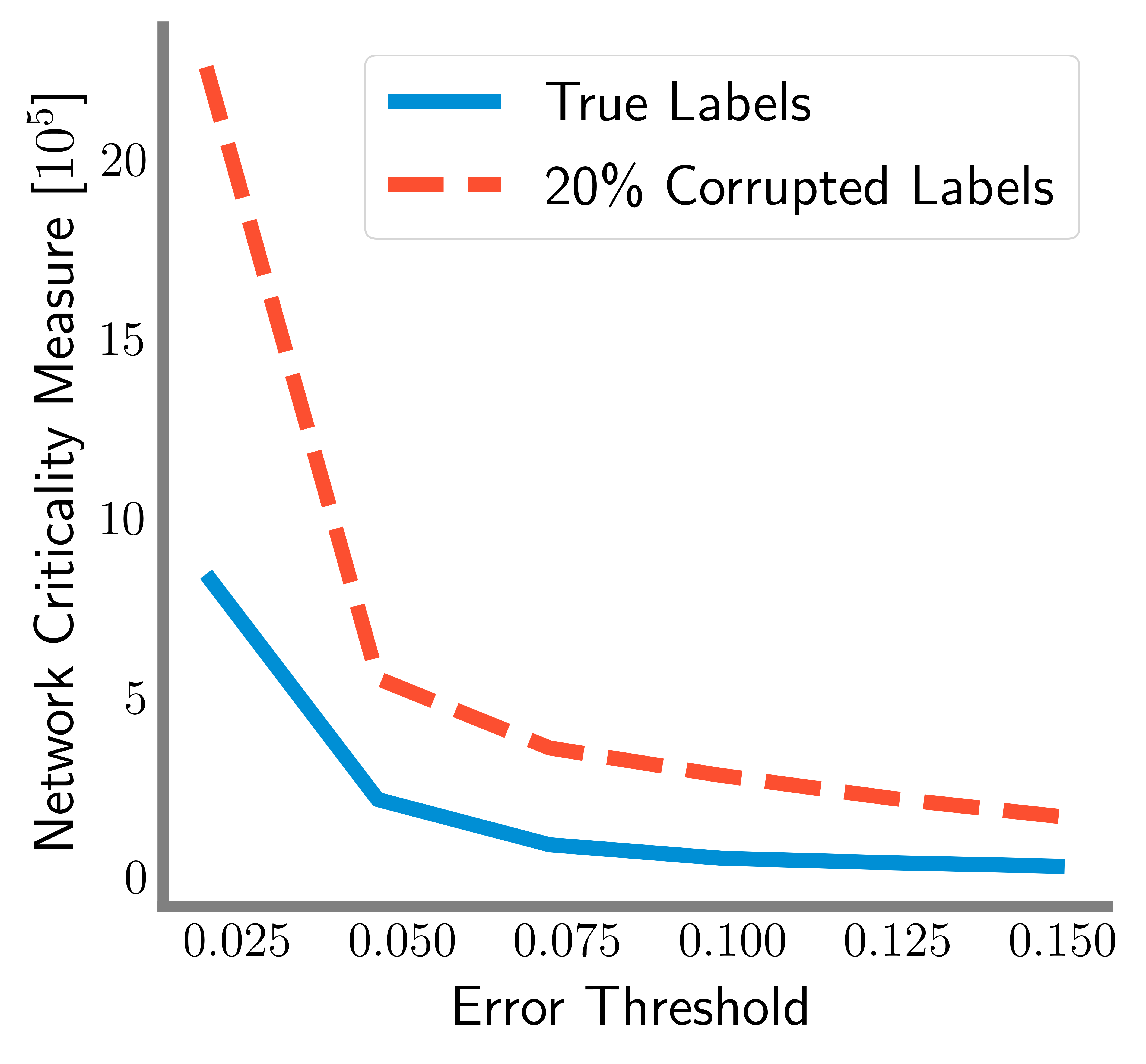
First, as a sanity check we use our complexity measure (lower is better) to compare between a ResNet18 trained on true labels and a ResNet18 trained on data where $20\%$ of the labels are randomly corrupted. As seen in Figure 5a, our measure is able to correctly capture that the network trained with true label generalizes better than the one trained on corrupted labels (4.62% error vs. 35% error).

(a) Comparing ResNet18 on trained true labels vs. corrupted labels

(b) Comparing ResNet18, ResNet34, VGG16 and FCN (I).

Figure 5: Network criticality as a function of error threshold for networks trained on CIFAR10.

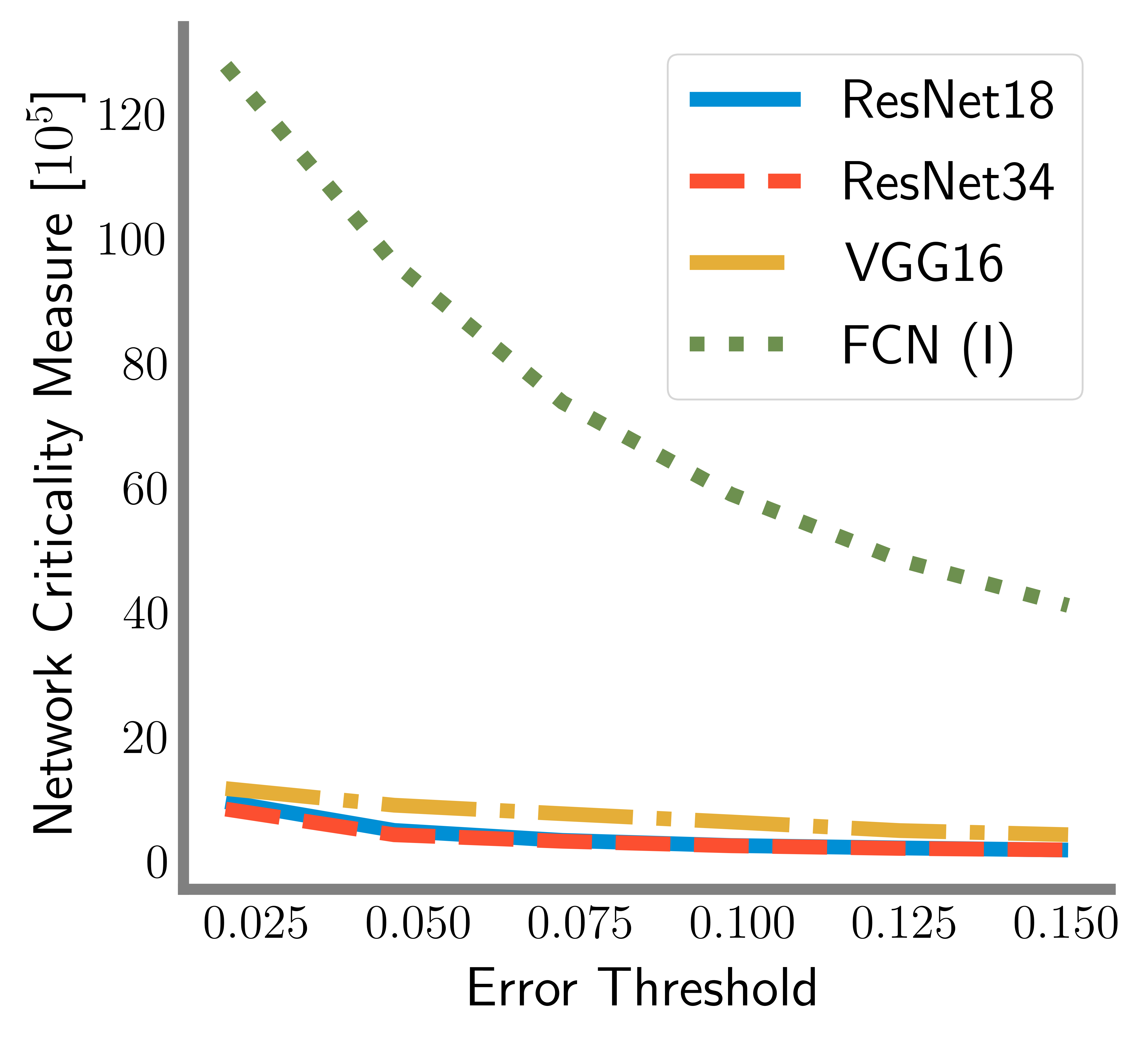
Next, in Table 2 we compare the generalization performance of several conventional DNN architectures trained on the CIFAR10 dataset. There is a particular ranking of the networks based on their generalization error and it is desirable for a complexity measure to capture this ranking. Therefore, we compare the rankings proposed by network criticality measure and complexity measures from the literature with the empirical rankings obtained in the experiment. To do this, we calculate the Kendall’s $\tau$ correlation coefficient (Kendall, 1938) which is defined as follows:

$$\text{Kendall's }\tau=\frac{\#\text{ of pairs where the rankings agree}-\#\text{ of pairs where the rankings disagree}}{\#\text{ pairs}}.$$

This coefficient lies between $-1$ and $1$, where $1$ denotes a high correlation between the two set of rankings. Table 2 shows that the Kendall’s $\tau$ coefficient between our network criticality measure and the generalization error is higher than all other complexity measures that we compared to.

We find that our measure correctly ranks the generalization performance of the networks – ResNet18, ResNet101, VGG16 and FCN (I). It fails to correctly identify the correct rank of ResNet34, ResNet50, DenseNet121, VGG11 and FCN (II).

We also repeat the above experiment for the same networks trained on the CIFAR100 dataset (see Table 3). We note that network criticality measure correctly predicts the ranking of generalization performance for ResNet101, ResNet34, ResNet18, ResNet50, VGG16 and the 3-layer fully connected networks (FCN). We find that the generalization error of ResNet101 is the lowest which is correctly captured only by our complexity measure and not by any other measure. Further, the Kendall’s $\tau$ correlation coefficient between the ranking based of the generalization error and our network criticality measure is 0.55 which is again higher than this coefficient for any other complexity measure. Our measure only fails to capture the ranking of VGG11 and DenseNet121 relative to the other DNN architectures and the relative ranking between FCN (I) and FCN (II).

Table 2: Measuring complexity of different architectures trained on CIFAR10.

Network	GE	PFN	PSN	DtI	NoP	SoSP	PAC Bayes	Net. Criticality
ResNet18	4.61%	1e22	4e14	3430	1.1e7	1.3e9	6.9e5	2.2e5
ResNet34	6.3%	2e37	3e24	4768	2.1e7	3.7e9	9.1e5	1.7e5
ResNet50	6.6%	4e56	4e20	10018	2.3e7	3.3e9	1.6e6	1.8e5
ResNet101	6.4%	8e110	3e32	18730	4.2e7	9.8e9	2.8e6	6.3e5
DenseNet121	7.8%	2e129	7e42	21359	6.8e6	2.0e9	1.2e6	4.1e5
VGG11	8.51%	1e11	1e6	2106	2.8e7	1.3e9	1.0e6	2.8e5
VGG16	7.47%	5e15	2e8	2341	3.4e7	2.1e9	1.2e6	2.70e5
FCN (I)	29.83%	3e20	2e7	75221	2.0e7	4.6e8	9.0e6	5.7e6
FCN (II)	26.45%	3e21	1e7	81258	5.0e7	2.0e9	9.5e6	6.2e6
Kendall’s $\tau$	-	-0.22	-0.33	0.38	0.16	-0.53	0.42	0.55

Table 3: Measuring complexity of different architectures trained on CIFAR100.

Network	GE	PFN	PSN	DtI	NoP	SoSP	PAC Bayes	Net. Criticality
ResNet18	30.6%	2e22	9e14	4855	1.1e7	1.4e9	3.4e6	1.6e6
ResNet34	29.3%	1e37	1e22	6017	2.1e7	3.6e9	6.7e6	1.4e6
ResNet50	31.1%	7e57	9e23	12715	2.3e7	4.1e9	5.8e6	1.9e6
ResNet101	25.5%	2e112	5e36	21233	4.2e7	1.1e10	6.4e6	1.3e6
DenseNet121	35.3%	1e131	1e49	23702	6.9e6	2.4e9	4.5e6	2.6e6
VGG11	43.5%	6e13	1e8	5059	2.8e7	1.7e9	3.6e6	2.4e5
VGG16	32.69%	8e19	4e12	7010	3.4e7	3.6e9	8.1e6	4.6e6
FCN (I)	57.59%	8e27	1e10	246636	2.0e7	8.3e8	2.4e7	1.2e7
FCN (II)	53.17%	1e29	1e10	329296	5.0e7	3.7e9	3.3e7	2.3e7
Kendall’s $\tau$	-	-0.27	-0.47	0.33	0	-0.42	0.22	0.55

We also perform an additional set of experiments in Appendix D where we calculate these complexity measures on four ResNet18 networks with changing channel widths.

5 Conclusion

In this paper, we studied the module criticality phenomenon and proposed a complexity measure based on module criticality that is able to correctly predict the superior performance of some DNN architectures over others, for a specific task. We believe module criticality can be used as a road-map for designing new task-specific architectures. Proposing new regularizers that improve generalization performance by bounding criticality or spreading it among various modules of the network is an exciting direction for future work. Our measure could also be potentially used in architecture search where we could calculate this score over the training set to select architectures that generalize well on the unseen test set.

Acknowledgements

We would like to thank Samy Bengio and Chiyuan Zhang for valuable conversations, and Yann Dauphin for his help with the implementation of Fixup initialization. We would also like to thank Chiyuan Zhang for sharing the code for the paper “Are all layers created equal?” Part of this work was performed while the author NC was an intern at Google AI, Brain team.

References

- Arora et al. (2018) Arora, S., R. Ge, B. Neyshabur, and Y. Zhang (2018). Stronger generalization bounds for deep nets via a compression approach. In Proceedings of the International Conference on Machine Learning.
- Bartlett (1998) Bartlett, P. (1998). The sample complexity of pattern classification with neural networks: the size of the weights is more important than the size of the network. IEEE Transactions on Information Theory 44(2), 525–536.
- Bartlett et al. (2017) Bartlett, P., D. Foster, and M. Telgarsky (2017). Spectrally-normalized margin bounds for neural networks. In Proceedings of the Advances in Neural Information Processing Systems.
- Baum and Haussler (1989) Baum, E. and D. Haussler (1989). What size net gives valid generalization? In Proceedings of the Advances in Neural Information Processing Systems.
- Dziugaite and Roy (2017) Dziugaite, G. K. and D. Roy (2017). Computing nonvacuous generalization bounds for deep (stochastic) neural networks with many more parameters than training data. In Proceedings of Uncertainity in Artificial Intelligence.
- He et al. (2015) He, K., X. Zhang, S. Ren, and J. Sun (2015). Delving deep into rectifiers: Surpassing human-level performance on imagenet classification. In Proceedings of the IEEE International Conference on Computer Vision.
- He et al. (2016) He, K., X. Zhang, S. Ren, and J. Sun (2016). Deep residual learning for image recognition. In Proceedings of the IEEE Conference on Computer Vision and Pattern Recognition.
- Huang et al. (2017) Huang, G., Z. Liu, L. Van Der Maaten, and K. Weinberger (2017). Densely connected convolutional networks. In Proceedings of the IEEE Conference on Computer Vision and Pattern Recognition.
- Kendall (1938) Kendall, M. (1938). A new measure of rank correlation. Biometrika 30(1/2), 81–93.
- Kingma and Ba (2014) Kingma, D. and J. Ba (2014). Adam: A method for stochastic optimization. arXiv preprint arXiv:1412.6980.
- Kornblith et al. (2019) Kornblith, S., M. Norouzi, H. Lee, and G. Hinton (2019). Similarity of neural network representations revisited. In Proceedings of the International Conference on Machine Learning.
- Kullback and Leibler (1951) Kullback, S. and R. Leibler (1951). On information and sufficiency. The Annals of Mathematical Statistics 22(1), 79–86.
- Langford and Caruana (2002) Langford, J. and R. Caruana (2002). (not) bounding the true error. In Proceedings of the Advances in Neural Information Processing Systems.
- Long and Sedghi (2019) Long, P. and H. Sedghi (2019). Generalization bounds for deep convolutional neural networks. arXiv preprint arXiv:1905.12600.
- McAllester (1999) McAllester, D. (1999). PAC-bayesian model averaging. In Proceedings of the Conference on Computational Learning Theory.
- Nagarajan and Kolter (2019a) Nagarajan, V. and Z. Kolter (2019a). Deterministic PAC-Bayesian generalization bounds for deep networks via generalizing noise-resilience. In Proceedings of the International Conference on Learning Representations.
- Nagarajan and Kolter (2019b) Nagarajan, V. and Z. Kolter (2019b). Generalization in deep networks: The role of distance from initialization. arXiv preprint arXiv:1901.01672.
- Neyshabur et al. (2017) Neyshabur, B., S. Bhojanapalli, D. McAllester, and N. Srebro (2017). Exploring generalization in deep learning. In Proceedings of the Advances in Neural Information Processing Systems.
- Neyshabur et al. (2018) Neyshabur, B., S. Bhojanapalli, and N. Srebro (2018). A PAC-Bayesian approach to spectrally-normalized margin bounds for neural networks. In Proceedings of the International Conference on Learning Representations.
- Neyshabur et al. (2019) Neyshabur, B., Z. Li, S. Bhojanapalli, Y. LeCun, and N. Srebro (2019). Towards understanding the role of over-parametrization in generalization of neural networks. In Proceedings of the International Conference on Learning Representations.
- Neyshabur et al. (2015) Neyshabur, B., R. Tomioka, and N. Srebro (2015). Norm-based capacity control in neural networks. In Proceedings of the Conference on Learning Theory.
- Pitas et al. (2017) Pitas, K., M. Davies, and P. Vandergheynst (2017). PAC-Bayesian margin bounds for convolutional neural networks. arXiv preprint arXiv:1801.00171.
- Sedghi et al. (2019) Sedghi, H., V. Gupta, and P. Long (2019). The singular values of convolutional layers. In Proceedings of the International Conference on Learning Representations.
- Simonyan and Zisserman (2015) Simonyan, K. and A. Zisserman (2015). Very deep convolutional networks for large-scale image recognition. In Proceedings of the International Conference on Learning Representations.
- Wei and Ma (2019) Wei, C. and T. Ma (2019). Data-dependent sample complexity of deep neural networks via Lipschitz augmentation. arXiv preprint arXiv:1905.03684.
- Zhang et al. (2019) Zhang, C., S. Bengio, and Y. Singer (2019). Are all layers created equal? arXiv preprint arXiv:1902.01996.
- Zhang et al. (2019) Zhang, H., Y. Dauphin, and T. Ma (2019). Residual learning without normalization via better initialization. In Proceedings of the International Conference on Learning Representations.
- Zhou et al. (2019) Zhou, W., V. Veitch, M. Austern, R. Adams, and P. Orbanz (2019). Non-vacuous generalization bounds at the imagenet scale: a PAC-Bayesian compression approach. In Proceedings of the International Conference on Learning Representations.
Appendix
Appendix A Proof of Thereorm 3.2
We start by stating the PAC-Bayes theorem which bounds the generalization error of any posterior distribution on parameters that can be reached using the training set given a prior distribution on parameters that should be chosen in advance and before observing the training set. Throughout this section given two scalar let denote the KL divergence between two Bernoulli distributions with success probabilities and respectively.
Theorem A.1 (McAllester (1999)).
For any data distribution , number of samples , training set , and prior distribution on parameters , posterior distribution , for any , with probability over the draw of training data we have that
where KL is the Kullback-Leibler (KL) divergence (Kullback and Leibler, 1951).
Following Dziugaite and Roy (2017), we use the inequality to achieve a simple bound on the test error:
The intuition from Figure 4 suggests that moving the parameters of each module as close as possible to the initialization value before harming performance. For such , we can then define the posterior for module to be a Gaussian distribution centered at with covariance matrix , that is, as if we have additive noise . We use to refer to the case where all are replaced with and matrix includes all . Then the training loss term can be decomposed as
where the second term on the right hand side of the inequality captures the flatness of the point by adding Gaussian noise and measuring the change in the loss. Therefore, searching over the posterior corresponds to finding a flat solution in the valley that connects the initial and final points. Next, we use this intuition to prove a generalization bound based on module criticality.
First, we express the value of the term in Theorem 3.2 , which is equal to as follows: