keywords: replicator dynamics, state based models, evolutionary game, stage structured population, age structured population, Owner-Intruder game

Abstract:
The paper contains the attempt to integration of the classical evolutionary game theory based on replicator dynamics and the state based approach of Houston and Mcnamara. In the new approach, individuals have different heritable strategies, however the individuals carrying the same strategy can differ on the state, role or situation in which they act. Thus, the

classical replicator dynamics is completed by the additional subsystem of differential equations describing the dynamics of transitions between different states. In effect the interactions described by game structure, in addition to the demographic payoffs (constituted by births and deaths) can lead to the change of state of the competing individuals. The special cases of the new framework of stage structured models where the state changes describe developmental steps or aging are derived. New approach is illustrated by the example of Owner-Intruder game with explicit dynamics of the role changes. New model is the generalization of the demographic version of the Hawk-Dove game, the difference is that opponents in the game are drawn from two separate subpopulations consisting of Owners and Intruders. Intruders check random nest sites, and play the Hawk-Dove game with the Owner if they are occupied. Interesting feedback mechanism is produced by fluxes of individuals between subpopulations. Owners produce newborns which become Intruders, since they should find a free nest site to reproduce.

1 Introduction

The classical evolutionary game theory consists of the game structure associated by replicator dynamics (Maynard Smith 1982; Cressman 1992; Hofbauer and Sigmund 1988, 1998) This approach is mainly based on the simple matrix games, where payoff matrices describe the excess from the average growth rate in the population for the respective strategies. To add necessary ecological details and to describe the models in measurable parameters, the classical approach was expressed in terms of the demographic vital rates (Argasinski and Broom 2013a, 2018a, 2018b; Zhang and Hui 2011; Huang et al. 2015, Gokhale and Hauert 2016). In this approach instead of single payoff function there are separate payoff functions describing the mortality (probability of death during interaction) and fertility (offspring number resulting from the interaction), in effect vital rates (birth and death rate) are products of interaction rates describing the distribution of interactions (game rounds) in time and demographic payoffs describing the average outcomes of a single interaction. Those mortality and survival payoff functions, describing the game interaction, may depend on each other leading to the trade-offs, such as mortality-fertility trade-off function describing the reproductive success of the survivors of the interaction (Argasinski and Broom 2013a, 2017, 2018). The distinction between opposing mortality and fertility forces was described as the cornerstone of the novel mechanistic formulation of evolutionary theory (Doebeli et al. 2017), however, the new approach is still based on a very strong simplifying assumption. The individuals (and thus their payoffs) differ only by inherited strategy and the individuals carrying the same strategy are completely equivalent. Another thing is that many conflicts in nature have no direct effect in the reproductive success or death, however they can affect the level of supplies of the individual. Thus births and deaths are not the only currency in which are paid payoffs in evolutionary games. The alternative general approach to the game theoretic modelling, dealing with the problem of non-heritable differences between individuals carrying the same genes was introduced in Houston and McNamara (1999). In the state based approach the individual differences caused by environmental conditions are explicitly taken into consideration. Independently, basic replicator dynamics models completed by state switching dynamics were introduced by Brunetti et al. (2015, 2018). The goal of this paper is to integrate the state based approach with the demographic approach to the dynamic evolutionary games (Argasinski and Broom 2013a, 2017, 2018). We will derive and analyze the general framework describing the dynamics underlying the process of state changes and the interplay between this process and the population dynamics. Some specific models dealing with the state or role changes already exist in literature. For example, dynamics of pair formation problem in Battle of the sexes (Myllius 1999), dynamics of role changes from Owner to Intruder caused by population feedbacks (Kokko et al. 2006) and formation of interacting pairs in games with time constraints (Křivan et al. 2018). However, the general game theoretic framework don’t contain tools allowing for modelling these problems. The last example (Křivan et al. 2018) is described as going ”beyond replicator dynamics”, but in this paper we want to show that replicator dynamics still can be useful for the problems of this type and it is too early to send it on retirement.

2 Methods

We will extend the event based approach of Argasinski and Broom (2013a,2017,2018) where individuals are involved in different activities (described as different evolutionary games) and the growth rate of the population is determined by the aggregated demographic outcomes of the particular events (rounds of different games). Then the growth of the population of the individuals with strategy $s$ can be presented as

$$\dot{n}_{s}=n_{s}\sum_{j}\tau^{j}\left(W_{s}^{j}-d_{s}^{j}\right)$$ (1)

where
$\tau^{j}$ is the interaction rate of $j$-th event (game type)
$W_{s}^{j}$ is the fertility payoff (number of offspring)
$d_{s}^{j}$ is the mortality payoff,

and products $\sum_{j}\tau^{j}W_{s}^{j}$ and $\sum_{j}\tau^{j}d_{s}^{j}$ constitute the demographic vital rates (Argasinski and Broom 2017). The strategy $s$ will affect payoffs in some particular types of games or in single type of game only, described as the focal game (for simplicity we will assume this case throughout the paper) with payoff functions $W_{s}^{F}$ and $d_{s}^{F}$. Then other games where all strategies will obtain equal payoffs will constitute background mortality and fertility rates:

$$W_{B} = \sum_{j}\tau_{B}^{j}W_{B}^{j}/\tau_{B}\text{ \ \ average fertility per event (where }\tau_{B}=\sum_{i}\tau_{B}^{i}\text{)}$$

$$m_{B} = \sum_{j}\tau_{B}^{j}d_{B}^{j}/\tau_{B}\text{ \ \ \ average death probability per event.}$$

Then equation (1) can be presented as

$$\dot{n}_{s}=n_{s}\left[\tau_{F}\left(W_{s}^{F}-d_{s}^{F}\right)+\tau_{B}\left(W_{B}-m_{B}\right)\right].$$ (2)

Then after adjustment of the timescale, the focal game occurrence rate can be removed from the equation. In effect background birth and death rates will be transformed into $\Phi=\frac{\tau_{B}}{\tau_{F}}W_{B}$ and $\Psi=\frac{\tau_{B}}{\tau_{F}}m_{B}$ leading to the simplified form of equations (2) where superscript $F$ is not necessary and the payoff functions can depend on the composition of the population described by the vector of strategy frequencies $q$ where$\ q_{s}=n_{s}/\sum_{i}n_{i}$:

$$\dot{n}_{s}=n_{s}\left[\left(W_{s}(q)-d_{s}(q)\right)+\left(\Phi-\Psi\right)\right].$$ (3)

Above system of equations can be transformed to the dynamics of the relative frequencies of the strategies by change of coordinates $q_{s}=n_{s}/\sum_{i}n_{i}$ leading to the replicator dynamics:

$$\dot{q}_{s}=q_{s}\left[\left(W_{s}(q)-\bar{W}(q)\right)-\left(d_{s}(q)-\bar{d}(q)\right)\right],$$ (4)

where $\bar{W}(q)=\sum_{s}q_{s}W_{s}(q)$ and $\bar{d}(q)=\sum_{s}q_{s}d_{s}(q)$. Note that background vital rates $\Phi$ and $\Psi$ vanishes from replicator dynamics. In more complicated cases, where individuals differ not only on strategies but also on some another trait such as for example sex (Argasinski 2012,2013,2017) we can use multipopulation  replicator dynamics (Argasinski 2006) where initial population is divided into some subpopulations. Then the composition of each subpopulation (indexed by superscript) described by frequencies $q_{s}^{j}=n_{s}^{j}/\sum_{j}n_{s}^{j}$ will be described by respective replicator dynamics (4). Those system of systems (4) will be completed by additional system describing the dynamics of relative proportions between those subpopulations $g_{s}=n_{s}/\sum_{j}n_{s}$ (where $n_{s}=\sum_{j}n_{s}^{j}$ and $n=\sum_{s}n_{s}$) which will have similar form to (4) but expressed in terms of the excess of the average subpopulation payoffs from average payoffs in the general population. The last element that should be added is the equation on general population size (scaling parameter). In effect we obtain

$$\dot{q}_{s}^{j} = q_{s}^{j}\left[\left(W_{s}^{j}(g,q)-\bar{W}_{s}(g,q)\right)-\left(d_{s}^{j}(g,q)-\bar{d}_{s}(g,q)\right)\right]$$ (5)

$$\dot{g}_{s} = g_{s}\left[\left(\bar{W}_{s}(g,q)-\bar{W}(g,q)\right)-\left(\bar{d}_{s}(g,q)-\bar{d}(g,q)\right)\right]$$

$$\dot{n} = n\left[\bar{W}(g,q)-\bar{d}(g,q)+\left(\Phi-\Psi\right)\right].$$

Respective demographic payoffs can depend on each other leading to the trade-off functions (Argasinski and Broom 2013a, 2017, 2018), for example when reproduction occurs after mortality stage, instead of simple fertility payoff $W_{s}$ we should use mortality-fertility trade-off function where $s_{i}^{j}(g,q)=1-d_{i}^{j}(g,q)$

$$V_{i}^{j}(g,q)=\sum_{l}q_{l}s_{i}^{j}(e_{l})W_{i}(e_{l}),$$ (6)

where only survivors of the game round can reproduce. The above system can be extended to explicit density dependence by some density dependent adult mortality or incorporation of the juvenile recruitment survival to the fertility payoffs (Argasinski and Broom 2013a, 2018a, 2018b). This can be implemented by multiplication of the fertility rates $W_{s}^{j}(g,q)$ or $V_{i}^{j}(g,q)$ by suppression coefficient $(1-n/K)$. Suppression can be interpreted as the juvenile recruitment survival. For constant mortality and fertility rates this approach leads to the Nest Site Lottery mechanism (Argasinski and Broom 2013b), where newborns introduced to the population compete for the available nest sites. Under shortage of nest sites they form the pool  of candidates from which are drawn those who replace dead adults in the released nest sites. It can work for other forms of suppression than logistic growth (Rudnicki 2018). The availability of nest sites can be used for derivation of the fully mechanistic growth model (Argasinski and Rudnicki 2017, Argasinski and Rudnicki submitted). This is important because changing juvenile survival alters the value of the reward in evolutionary games (Argasinski and Broom 2013a, 2018a, 2018b) which may invert the strategic situation leading to breakdown of the growth of some strategy (Argasinski and Broom 2013a) or even stabilize the unstable invasion barrier (Argasinski and Broom 2018b). The general impact of the density dependence on selection deserves more attention (Dańko et al 2018).

3 Results

$n_{s}^{i}$   number of individuals with strategy $s$ and in state $i$
$q_{s}^{i}=n_{s}^{i}/\sum_{j}n_{j}^{i}$   frequency of individuals in state $i$ among $s$-strategists
$g_{s}=\sum_{i}n_{s}^{i}/\sum_{z}\sum_{l}n_{z}^{l}$   frequency of $s$-strategists in the population
$\tau^{j}$   is the interaction rate of $j$-th event (game type)
$W_{s}^{i}$   is the fertility payoff (number of offspring) of $s$-strategist in state $i$
$d_{s}^{i}$    is the mortality payoff of $s$-strategist in state $i$
$\Phi^{i}$   background fertility rate in state $i$
$\Psi^{i}$   background mortality rate in state $i$
$c_{s}^{i,z}(g,q)$    switching payoff (probability of transition from state $i$ to $z$ )
$c_{s}^{i}=\sum_{k\neq i}c_{s}^{i,k}=1-c_{s}^{i,i}$    probability of leaving the state $i$
$\Lambda^{z,i}$    background switching rate
$\Lambda^{i}$      background leaving rate
$V_{s}^{i}(q,g)$    survival-fertility trade-off function
$Z_{s}^{i,j}(q,g)$   survival-switching trade-off function
$X_{s}^{i}(q,g)$    switching-survival trade-off function
$Y_{s}^{i}(q,g)$    switching-mortality trade-off function
$\bar{W}_{s}(g,q)$, $\bar{W}(g,q)$   average fertility payoff of $s$-strategists/whole population
$\bar{s}_{s}(g,q)$, $\bar{s}(g,q)$     average survival payoff of $s$-strategists/whole population
$\bar{c}_{s}(g,q)$, $\bar{c}(g,q)$     average switching payoff of $s$-strategists/whole population
$\bar{\Phi}_{s}(q_{s})$, $\bar{\Phi}(g,q)$     average background fertility rate of $s$-strategists/whole population
$\bar{\Psi}_{s}(q_{s})$, $\bar{\Psi}(g,q)$   average background mortality rate of $s$-strategists/whole population
$\bar{\Lambda}^{i}$, $\bar{\Lambda}$    average background leaving rate of state $i$/whole population
$H^{O}$, $H^{I}$    proportion of Hawks among Owners/Intruders
$\Phi_{s}^{I}=\frac{q_{s}^{O}}{1-q_{s}^{O}}\Phi$ Intruders per capita increase rate caused by Owners background fertility

Table 1 List of important symbols

Plan of the paper:
-completion of the framework presented in introduction by switching payoffs describing state changes resulting from the game (sections 3.1-3.2).
-introduction of the trade-off functions analogous to the mortality-fertility trade-off function (6) describing the trade-offs between demographic payoffs and switching payoffs (section 3.3).
-introduction of ratio dependent nonuniform interaction rates, when interactions occur between individuals in different states (Males and Females or Owners with Intruders), section 3.4.
-derivation of the generalized replicator dynamics, where selection equations are completed by equations describing the dynamics of fluxes between different states among carriers of different strategies (sections 3.5-3.8), including the limit cases of separation of timescales between switching and demographic dynamics (section 3.9).
-special cases of the obtained framework describing the stage and age structured populations (section 4).
-example of Owner-Intruder game describing the competition for nest sites, with explicit dynamics of fluxes between roles of settled Owner and homeless Intruder.

3.1 Population growth with switching payoffs

Here we will extend the framework from the previous section to the state dependent case. Table 1 contains list of important symbols. Therefore, assume that individuals in the population differ in states and similarly to the previous section are involved in the different types of events, described by demographic outcomes (mortality and fertility). Then each type of interaction event can be characterized by following parameters:

$\tau^{j}$ is the interaction rate of $j$-th event, since it is not affected by state.
$d_{s,i}^{j}$ is the mortality payoff (probability of death during interaction event)
$W_{s,i}^{j}$ is the fertility payoff (number of offspring resulting from the interaction)
of $s$-strategist in state $i$ obtained in $j$th type event.

However, state is not heritable, offspring may have different state than parental individual. We can assume that the state of the offspring is drawn with the probability $\zeta_{s,i}(k)$ for $k$-th state. Then individual $s,i$ will produce $O_{s,i}^{j}\zeta_{s,i}(k)$ individuals in state $k$ (where $O_{s,i}^{j}$ is the mating payoff which describes the number of offspring obtained by $s,i$ in the $j$-th type event). Then $\sum_{z}n_{s,z}O_{s,z}^{j}\zeta_{s,z}(k)$ individuals in state $k$ will be produced leading to the following average aggregated per capita fertility rate of individual $s,i$ caused by the $j$-th type of event:

$$W_{s,i}^{j}=\dfrac{\sum_{z}n_{s,z}O_{s,z}^{j}\zeta_{s,z}(i)}{n_{s,i}}$$ (7)

and $O_{s,i}^{j}$ is the mating payoff (successful mating attempts). The general growth equation equivalent to (1) of the subpopulation of individuals in state $i$ and with strategy $s$ (described by the subscript vector $s,i$ while superscripts will describe event type will be:

$$\dot{n}_{s,i}=n_{s,i}\sum_{j}\tau^{j}\left(W_{s,i}^{j}-d_{s,i}^{j}\right)$$ (8)

We should add the third type of the event outcome, the probability of switch in the state from $i$ to $k$ (for $i\neq k$) described by $c_{s,i,k}^{j}$ (assume that $c_{s,i}^{j}=\sum_{k\neq i}c_{s,i,k}^{j}=1-c_{s,i,i}^{j}$ describes the per capita probability of leaving the state $i$). This idea is similar to the state switching dynamics introduced by Brunetti et al. (2015, 2018). Then the population should be divided into different state classes. Then we should update our equation to the following form where term $\sum_{j}n_{i}\tau^{j}c_{s,i}^{j}$ describes the leaving rate, i.e. changes of a state of the individuals in the $i$-th state, while term $\sum_{j}\sum_{z}n_{z}\tau^{j}c_{s,z,i}^{j}$ describes the incoming rate, per capita increase of individuals in state $i$ caused by switches of individuals at the other states.

$$\dot{n}_{s,i} = \sum_{j}n_{s,i}\tau^{j}\left(W_{s,i}^{j}-d_{s,i}^{j}\right)-n_{s,i}\sum_{j}\tau^{j}c_{s,i}^{j}+\sum_{j}\sum_{z\neq i}n_{s,z}\tau^{j}c_{s,z,i}^{j}$$

$$= n_{s,i}\left[\sum_{j}\tau^{j}\left(W_{s,i}^{j}-d_{s,i}^{j}\right)+\sum_{j}\tau^{j}\left(\sum_{z\neq i}\dfrac{n_{s,z}}{n_{s,i}}c_{s,z,i}^{j}-\sum_{j}c_{s,i}^{j}\right)\right]$$

3.2 Extraction of the focal type of interaction

Now we can extract focal interactions affected by analyzed trait from the general dynamics and assume that they are functions of the population composition i.e. game payoffs. The population state is described by vector $(q_{s,i},g_{s})$:

$q_{s,i}=n_{s,i}/\sum_{l}n_{s,l}$ state distributions among carriers of the particular strategies

$g_{s}=\sum_{i}n_{s,i}/\sum_{z}\sum_{l}n_{z,l}$   strategy frequencies

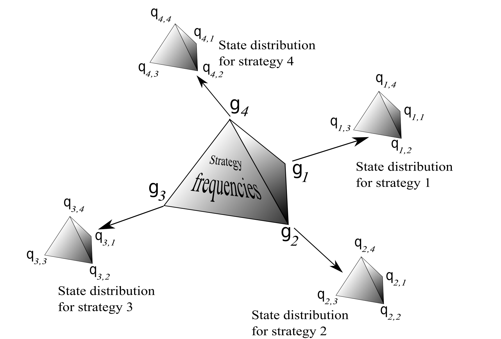
Figure 1: Schematic presentation of the phase space of the system

See fig.1 for the schematic presentation of the phase space. Individuals enter an focal game (with payoffs $W_{s,i}^{F}(g,q)$ and $d_{s,i}^{F}(g,q)$ where auxiliary index $F$ means ”focal event”) at rate $\tau_{F}$ as in equation (8), and engage in other activities at rates described by $\tau_{B}^{i}$; we can consider a single class of all such activities, as we show below. Assume that background events do not depend on the strategies but are affected by state, since for example energy level will have impact on the overall performance of the organism. Each of the background events can be characterized by outcomes which include a fertility $W_{B,i}^{j}$ and mortality $d_{B,i}^{j}$ (lower index $B$ means ”background event”). We should also consider the background switching dynamics where

$$c_{B,z,i}=\sum_{j}\tau_{B}^{j}c_{B,z,i}^{j}/\tau_{B}\text{ \ \ \ and \ \ \ \ \ }c_{B,i}=\sum_{j}\tau_{B}^{j}c_{B,i}^{j}\text{,}$$

because it will be affected by the actual state distribution determined by impact of the focal game. We can calculate the outcomes of the average background event for the individual in state $i$:

$$W_{B,i} = \sum_{j}\tau_{B}^{j}W_{B,i}^{j}/\tau_{B}\text{ \ \ average fertility per event (where }\tau_{B}=\sum_{i}\tau_{B}^{i}\text{)}$$

$$m_{B,i} = \sum_{j}\tau_{B}^{j}d_{B,i}^{j}/\tau_{B}\text{ \ \ \ average death probability per event.}$$

In effect “background events” occur at intensity $\tau_{B}$ and individuals involved in those events obtain fertility $W_{B,i}$ on average and die with probability $m_{B,i}$. Then equation (8) can be presented similarly to (2) in the form:

$$\dot{n}_{s,i} = n_{s,i}\tau_{F}\left[\left(W_{s,i}^{F}(g,q)-d_{s,i}^{F}(g,q)\right)+\left(\sum_{z\neq i}\dfrac{n_{s,z}}{n_{s,i}}c_{s,z,i}^{F}(g,q)-c_{s,i}^{F}(g,q)\right)\right]$$ (10)

$$+n_{s,i}\tau_{B}\left[\left(W_{B,i}-m_{B,i}\right)+\left(\sum_{z\neq i}\dfrac{n_{s,z}}{n_{s,i}}c_{B,z,i}-c_{B,i}\right)\right].$$

We can adjust the timescale to make the focal game’s vital rates equal to their demographic payoffs. This will keep the mechanistic interpretation as the number of offspring and the death probability during the interaction event. It is clear that only the ratio of our two interaction rates is important for the evolution of the population. Similarly to (3), after a change of timescale $\tilde{t}=t\tau_{F}$, $\tau_{F}$ vanishes and $\tau_{B}$ transforms into $\theta=\dfrac{\tau_{B}}{\tau_{F}}$. Since demographic parameters $W_{B,i}$ and $m_{B,i}$ never occur without the ratio between intensities $\theta$, we can simplify this by substitutions $\Phi^{i}=\theta W_{B,i}$ and $\ \Psi^{i}=\theta m_{B,i}$, constituting the background vital rates. In similar way we can derive the background switching intensities $\Lambda^{z,i}=\theta c_{B,z,i}$ and respectively $\Lambda^{i}=\theta c_{B,i}$ This leads to:

$$\dot{n}_{s,i} = n_{s,i}\left[\left(W_{s,i}^{F}(g,q)-d_{s,i}^{F}(g,q)\right)+\left(\sum_{z\neq i}\dfrac{n_{s,z}}{n_{s,i}}c_{s,z,i}^{F}(g,q)-c_{s,i}^{F}(g,q)\right)\right]$$ (11)

$$\text{ \ }+n_{s,i}\left[\left(\Phi^{i}-\Psi^{i}\right)+\left(\sum_{z\neq i}\dfrac{n_{s,z}}{n_{s,i}}\Lambda^{z,i}-\Lambda^{i}\right)\right].$$

Since we extracted the focal interaction and averaged the background interactions, we can simplify the notation by removing the superscript $F$, since it is not necessary now. We can assume that from now subscript describes the strategy while superscript describes the state. This leads to the following general growth equation:

$$\dot{n}_{s}^{i} = {}n_{s}^{i}\left[\left(W_{s}^{i}(g,q)-d_{s}^{i}(g,q)\right)+\left(\sum_{z\neq i}\dfrac{n_{s}^{z}}{n_{s}^{i}}c_{s}^{z,i}(g,q)-c_{s}^{i}(g,q)\right)\right]$$ (12)

$$+n_{s}^{i}\left[\left(\Phi^{i}-\Psi^{i}\right)+\left(\sum_{z\neq i}\dfrac{n_{s}^{z}}{n_{s}^{i}}\Lambda^{z,i}-\Lambda^{i}\right)\right].$$

3.3 Causal structure of the focal interaction

Following Argasinski and Broom (2012) we can describe the order of the different outcomes of the focal interaction. For example only survivors of the interaction can reproduce. Then we have survival payoff function $s_{s}^{i}(q,g)=1-d_{s}^{i}(q,g)$. To derive the mortality-fertility trade-off function where reproductive success of survivors is described by product of survival and fertility $s_{s}^{i}W_{s}^{i}$ (Argasinski and Broom, 2012), outcomes of interactions with all strategies present in the population should be averaged. Recall that the population state is described by set of vectors $\left[g,q\right]$ where $q$ consists of vectors of state distributions $q_{s}$ for all strategies. Monomorphic uniform population consisting of $s$ strategists in state $i$ , where $q_{s}^{i}=g_{s}=1$ and all other entries are zeros, can be described by state vector $u_{s}^{i}=[e_{s},e_{s}^{i}]$ where $e_{s}$ is the unit vector for argument $g_{s}$ and $e_{s}^{i}$ is the unit vector with $1$ on $i$th place for argument $q_{s}^{i}$, state distribution vectors $q_{j\neq s}^{i}$ for other strategies are zeros. It can be used as an argument of the payoff functions to simplify the notation. Then for example $s_{s}^{i}(u_{k}^{l})$ will describe survival of $s$ strategists in state $i$ playing with $k$th strategy carrier in state $l$. Then the mortality-fertility trade-off equivalent to (6) function will be:

$$V_{s}^{i}(q,g)=\sum_{k}g_{k}\sum_{l}q_{k}^{l}s_{s}^{i}(u_{k}^{l})W_{s}^{i}(u_{k}^{l})$$

similarly when only survivors of the interaction can switch to another state we can introduce the survival-switching trade-off function

$$Z_{s}^{i,j}(q,g)=\sum_{k}g_{k}\sum_{l}q_{k}^{l}s_{s}^{i}(u_{k}^{l})c_{s}^{i,j}(u_{k}^{l})$$ (13)

that will replace functions $c_{s}^{i,j}$ in the equations from previous sections. Then the function $c_{s}^{i}$ describing the probability of leaving the state $i$ should be replaced by

$$Z_{s}^{i}(q,g) = \sum_{j\neq i}Z_{s}^{i,j}(q,g)=\sum_{k}g_{k}\sum_{l}q_{k}^{l}s_{s}^{i}(u_{k}^{l})\sum_{j\neq i}c_{s}^{i,j}(u_{k}^{l})$$

$$= \sum_{k}g_{k}\sum_{l}q_{k}^{l}s_{s}^{i}(u_{k}^{l})c_{s}^{i}(u_{k}^{l}).$$

We can also imagine the situation that mortality acts after the state switching (thus only those individuals will die which remained in the focal state) leading to switching-survival trade-off function

$$X_{s}^{i}(q,g)=\sum_{k}g_{k}\sum_{l}q_{k}^{l}\left[1-c_{s}^{i}(u_{k}^{l})\right]s_{s}^{i}(u_{k}^{l})=1-Z_{s}^{i}(q,g)$$ (14)

that will replace functions $s_{s}^{i}$ and then the switching-mortality trade-off function, equivalent to $d_{s}^{i}=(1-s_{s}^{i})$ will be

$$Y_{s}^{i}(q,g) = \sum_{k}g_{k}\sum_{l}q_{k}^{l}\left[1-c_{s}^{j}(u_{k}^{l})\right]d_{s}^{i}(u_{k}^{l})$$

$$= \sum_{k}g_{k}\sum_{l}q_{k}^{l}\left[1-c_{s}^{i}(u_{k}^{l})\right]-X_{s}^{i}(q,g)$$

$$= Z_{s}^{i}(q,g)-\sum_{k}g_{k}\sum_{l}q_{k}^{l}c_{s}^{i}(u_{k}^{l}).$$

Note that since $d_{i}^{j}=(1-s_{i}^{j})$ we have

$$X_{s}^{i}+Y_{s}^{i}=\sum_{k}g_{k}\sum_{l}q_{k}^{l}\left[1-c_{s}^{i}(u_{k}^{l})\right],$$

which describes the average probability of remaining in the same state.

3.4 Frequency dependence and the interaction rates

Note that the respective payoff functions presented above describe outcomes of the average focal interaction. The argument of those functions should be vector of the population state describing distribution of states for all strategies $q_{j}^{i}$ and the strategy frequencies $g_{i}$. This will be enough for description of the frequency dependent selection among randomly paired individuals with different strategies and states. However, this is not the only case. We can imagine situation, when interactions occur only between individuals in different particular states (such as when owners of the habitat interact only with the intruders). In the simplest ”gas” model of panmictic population of randomly meeting individuals this can be realized by assumption that only interactions between those particular types have nonzero payoffs. However, we can imagine situations when pairing is not completely random, such as mating when males search for females or owner-intruder problem when homeless individuals investigate the nest-sites. Then random pairing is limited to drawing opponents from opposite subgroups. Then pure frequency dependence should be completed by the impact of the proportion between interacting subpopulations. This is important, because if the ratio between interacting subgroups is not 1, than individuals from different subgroups will have different chances of interactions determined by availability of potential opponents/partners. This will result in different average numbers of interactions for different types (this will be shown later by Owner-Intruder example). Therefore, we cannot limit ourselves to description of the average outcomes of interaction only. This may lead to badly defined models, similarly to the case of bimatrix games, which are independent of the proportion between playing subpopulations (Argasinski 2006). Different numbers of interactions for different types/states can be described by resulting different interaction rates (Argasinski and Broom 2017). For example if we have asymmetric pairwise interactions between individuals acting in two opposite roles (such as Owner-Intruder conflict) and the distribution of states is described by $q_{i}^{j}$ for $it$h strategy in the $j$th role. Then, on average, ratio of individuals in role 1 to individuals in role 2 is $\sum_{s}g_{s}q_{s}^{1}/\sum_{s}g_{s}(1-q_{s}^{1})$ and it is proportional to the ratio of per capita interaction rates for both roles, since individuals in minority will always find the opponent, while those in majority not, due to shortage of individuals of the opposite type. Thus, for example, if for minority type we have $\tau_{F}^{1}=1$ then for majority type we have $\tau_{F}^{2}=\sum_{i}g_{i}q_{i}^{1}/\sum_{i}g_{i}q_{i}^{2}$. Then, for example, the respective death rates in (12), and in the resulting replicator equations, will be

$$D_{i}^{1}(g,q)=d_{i}^{1}(g,q)=1-s_{i}^{1}(g,q)\text{ \ \ for \ \ role \ \ 1 }$$ (15)

$$D_{i}^{2}(g,q)=d_{i}^{2}(g,q)\dfrac{\sum_{i}g_{i}q_{i}^{1}}{\sum_{i}g_{i}(1-q_{i}^{1})}=\left(1-s_{i}^{2}(g,q)\right)\dfrac{\sum_{i}g_{i}q_{i}^{1}}{\sum_{i}g_{i}(1-q_{i}^{1})}\text{ \ \ for role 2}$$ (16)

If the interaction rate decreases due to the shortage of the opponents of the opposite type we have following interaction rates

$$\tau_{F}^{1} = \left\{\begin{array}[]{c}1\text{ \ \ \ \ \ \ \ \ \ \ \ \ \ \ \ \ \ \ \ for\ \ \ \ \ \ \ \ }\dfrac{\sum_{i}g_{i}q_{i}^{1}}{\sum_{i}g_{i}(1-q_{i}^{1})}\leq 1\\ \dfrac{\sum_{i}g_{i}(1-q_{i}^{1})}{\sum_{i}g_{i}q_{i}^{1}}\text{ \ \ \ for \ \ \ \ \ }\dfrac{\sum_{i}g_{i}q_{i}^{1}}{\sum_{i}g_{i}(1-q_{i}^{1})}>1\end{array}\right.$$ (19)

$$\tau_{F}^{2} = \left\{\begin{array}[]{c}\dfrac{\sum_{i}g_{i}q_{i}^{1}}{\sum_{i}g_{i}(1-q_{i}^{1})}\text{ \ \ \ for \ \ \ \ \ }\dfrac{\sum_{i}g_{i}q_{i}^{1}}{\sum_{i}g_{i}(1-q_{i}^{1})}\leq 1\\ 1\text{ \ \ \ \ \ \ \ \ \ \ \ \ \ \ \ \ \ for\ \ \ \ \ \ \ \ \ \ \ }\dfrac{\sum_{i}g_{i}q_{i}^{1}}{\sum_{i}g_{i}(1-q_{i}^{1})}>1\end{array}\right.,$$ (22)

and due to previous derivation based on the change of the timescale, it will act as the multiplicative factor on the r.h.s. of (12). Similarly, difference in the interaction rates for different states/types should be incorporated into switching payoffs constituting switching rates and the trade-off functions constituting conditional fertility and death rates and conditional switching. In the next sections we will limit ourselves to the basic simple demographic and switching rates and focus on the dynamics. When it is necessary, simple payoff functions will be replaced by more detailed tradeoff functions and nontrivial interaction rates described in this and in the previous section.

3.5 Derivation of the replicator dynamics

We will use the multipopulation approach (5) to replicator dynamics (Argasinski 2006, 2012, 2013, 2018), where population can be decomposed into subpopulations described by their own replicator dynamics. Subsystems describing those subpopulations are completed by additional set of replicator equations describing the dynamics of proportions of all subpopulations. Then we can describe the distribution of states among $s$-strategists in related frequencies $q_{s}^{i}=n_{s}^{i}/\sum_{j}n_{s}^{j}$. In effect, fertility payoff (7) of the focal game can be presented in the new indexing convention and in frequencies as:

$$W_{s}^{i}(g,q)=\dfrac{\sum_{z}n_{s}^{z}O_{s}^{z}(g,q)\zeta_{s}^{z}(i)}{n_{s}^{i}}=\dfrac{\sum_{z}q_{s}^{z}O_{s}^{z}(g,q)\zeta_{s}^{z}(i)}{q_{s}^{i}}$$ (23)

Now we can derive the replicator dynamics, in a standard way, by rescaling the growth equations $\dot{n}_{i}=n_{i}r_{i}=n_{i}\left(W_{i}-d_{i}\right)$ (where $r_{i}$ is the function describing growth rate) into frequency equations (4) which have form $\dot{q}_{i}=q_{i}\left(r_{i}-\sum_{k}q_{k}r_{k}\right)=q_{i}\left(\left[W_{i}-\sum_{k}q_{k}W_{k}\right]-\left[d_{i}-\sum_{k}q_{k}d_{k}\right]\right)$, describing the changes of distribution of the states for the $i$-th strategy, completed by total population size equation $\dot{n}=n\sum_{i}q_{i}r_{i}$. Since

$$\sum_{z\neq i}\dfrac{n_{s}^{z}}{n_{s}^{i}}c_{s}^{z,i}(g,q)=\sum_{z\neq i}\dfrac{q_{s}^{z}}{q_{s}^{i}}c_{s}^{z,i}(g,q)\ \ \ \ \text{and}\ \ \ \ \ \sum_{i}q_{s}^{i}\sum_{z\neq i}\dfrac{q_{s}^{z}}{q_{s}^{i}}c_{s}^{z,i}(g,q)=\sum_{i}\sum_{z\neq i}q_{s}^{z}c_{s}^{z,i}(g,q)$$ (24)

the respective bracketed term will be

$$q_{s}^{i}\left(\sum_{z\neq i}\dfrac{q_{s}^{z}}{q_{s}^{i}}c_{s}^{z,i}(g,q)-\sum_{k}\sum_{z\neq k}q_{s}^{z}c_{s}^{z,k}(g,q)\right),$$

similarly for $\Lambda$ terms. Then we will obtain:

$$\dot{q}_{s}^{i} = {}q_{s}^{i}\left[\left(W_{s}^{i}(g,q)-\bar{W}_{s}(g,q)\right)-\left(d_{s}^{i}(g,q)-\bar{d}_{s}(g,q)\right)+\left(\Phi^{i}-\bar{\Phi}_{s}(q_{s})\right)\right.$$ (25)

$$\left.-\left(\Psi^{i}-\bar{\Psi}_{s}(q_{s})\right)-\left(c_{s}^{i}(g,q)-\bar{c}_{s}(g,q)\right)-\left(\Lambda^{i}-\bar{\Lambda}(q_{s})\right)\right]$$

$$+\left(\sum_{z\neq i}q_{s}^{z}c_{s}^{z,i}(g,q)-q_{s}^{i}\sum_{k}\sum_{z\neq k}q_{s}^{z}c_{s}^{z,k}(g,q)\right)$$

$$+\left(\sum_{z\neq i}q_{s}^{z}\Lambda^{z,i}-q_{s}^{i}\sum_{k}\sum_{z\neq k}q_{s}^{z}\Lambda^{z,k}\right),$$

where

$$\bar{W}_{s}(g,q) = \sum_{k}q_{s}^{k}W_{s}^{k}(g,q),\quad\bar{d}_{s}(g,q)=\sum_{k}q_{s}^{k}d_{s}^{k}(g,q),$$

$$\bar{\Phi}_{s}(q_{s}) = \sum_{k}q_{s}^{k}\Phi^{k},\quad\bar{\Psi}_{s}(q_{s})=\sum_{k}q_{s}^{k}\Psi^{k},$$

$$\bar{c}_{s}(g,q) = \sum_{k}q_{s}^{k}c_{s}^{k}(g,q),\quad\text{and $\bar{\Lambda}(q_{s})=\sum_{k}q_{s}^{k}\Lambda^{k}$}.$$

3.6 Case of two competing strategies

In the special case where for all strategies we have only two states, the above system reduces to the single equation. In addition it can be simplified by application of well known form of the replicator dynamics for two strategies $\dot{q}_{1}=q_{1}(1-q_{1})\left[r_{1}-r_{2}\right]$.  In addition the terms describing the switching dynamics in (24) will be also simplified and for both states will have forms

$$\sum_{z\neq 1}\dfrac{n_{s}^{z}}{n_{s}^{1}}c_{s}^{z,1}(g,q) = \dfrac{\left(1-q_{s}^{1}\right)}{q_{s}^{1}}c_{s}^{2,1}(g,q)$$

$$\sum_{z\neq 2}\dfrac{n_{s}^{z}}{n_{s}^{2}}c_{s}^{z,2}(g,q) = \dfrac{q_{s}^{1}}{\left(1-q_{s}^{1}\right)}c_{s}^{1,2}(g,q),$$

leaving rates $c_{s}^{i}(g,q)$ reduce to

$$c_{s}^{1}(g,q)=c_{s}^{1,2}(g,q)\text{ \ \ \ and \ \ }c_{s}^{1}(g,q)=c_{s}^{1,2}(g,q).$$

since there is only single opposite state to switch. Then the external bracketed term describing the impact of switching dynamics will be:

$$q_{s}^{1}\left(1-q_{s}^{1}\right)\left(\left[\dfrac{\left(1-q_{s}^{1}\right)}{q_{s}^{1}}c_{s}^{2,1}(g,q)-c_{s}^{1,2}(g,q)\right]-\left[\dfrac{q_{s}^{1}}{\left(1-q_{s}^{1}\right)}c_{s}^{1,2}(g,q)-c_{s}^{2,1}(g,q)\right]\right)$$

$$= \left(1-q_{s}^{1}\right)\left[\left(1-q_{s}^{1}\right)c_{s}^{2,1}(g,q)-q_{s}^{1}c_{s}^{1,2}(g,q)\right]+q_{s}^{1}\left[\left(1-q_{s}^{1}\right)c_{s}^{2,1}(g,q)-q_{s}^{1}c_{s}^{1,2}(g,q)\right]$$

$$= \left(1-q_{s}^{1}\right)c_{s}^{2,1}(g,q)-q_{s}^{1}c_{s}^{1,2}(g,q)$$

Similar form will have terms describing the background switching dynamics. Then the equation describing the transitions between two states will be:

$$\dot{q}_{s}^{1}=q_{s}^{1}\left(1-q_{s}^{1}\right)\left[\left(W_{s}^{1}(g,q)-W_{s}^{2}(g,q)\right)-\left(d_{s}^{1}(g,q)-d_{s}^{2}(g,q)\right)+\left(\Phi^{1}-\Phi^{2}\right)-\left(\Psi^{1}-\Psi^{2}\right)\right]$$

$$\,\,+\left[\left(1-q_{s}^{1}\right)c_{s}^{2,1}(g,q)-q_{s}^{1}c_{s}^{1,2}(g,q)\right]+\left[\left(1-q_{s}^{1}\right)\Lambda^{2,1}(g,q)-q_{s}^{1}\Lambda^{1,2}(g,q)\right],$$ (26)

and the averaged values are not necessary.

3.7 Selection of the strategies

Now we can describe the selection of strategies by application of the multipopulation approach 5). Then the above system  ((25) or (26))should be completed by the additional set of the replicator equations describing the related frequencies of the other strategies. Obviously the dynamics of state changes will not have direct impact on the strategy frequencies (as well as on the population size) since it will not change the number of strategy carriers. Then we have the following system describing the selection:

$$\dot{g}_{s}={}g_{s}\left[\left(\bar{W}_{s}(g,q)-\bar{W}(g,q)\right)-\left(\bar{d}_{s}(g,q)-\bar{d}(g,q)\right)\right.\\ \left.+\left(\bar{\Phi}_{s}(q_{s})-\bar{\Phi}(g,q)\right)-\left(\bar{\Psi}_{s}(q_{s})-\bar{\Psi}(g,q)\right)\right],$$ (27)

where

$$\bar{W}(g,q) = \sum_{k}g_{k}\bar{W}_{k}(g,q),\quad\bar{d}(g,q)=\sum_{k}g_{k}\bar{d}_{k}(g,q),$$

$$\bar{\Phi}(g,q) = \sum_{k}g_{k}\bar{\Phi}_{k}(q_{k}),\quad\bar{\Psi}(g,q)=\sum_{k}g_{k}\bar{\Psi}_{k}(q_{k}).$$

The above system should be completed by the equation on total population size:

$$\dot{n}=n\left[\bar{W}(g,q)-\bar{d}(g,q)+\bar{\Phi}(g,q)-\bar{\Psi}(g,q)\right]$$ (28)

Note that for the uniform interaction rate $\tau_{F}$ for all strategies the negative mortality bracketed terms $\left(\bar{d}_{s}(g,q)-\bar{d}(g,q)\right)$ and $\left(d_{s}^{1}(g,q)-d_{s}^{2}(g,q)\right)$ reduce to the positive bracketed terms $\left(\bar{s}_{s}(g,q)-\bar{s}(g,q)\right)$ and $\left(s_{s}^{1}(g,q)-s_{s}^{2}(g,q)\right)$. this will not work for nonuniform interaction rates. The above system can be easily extended to density dependence by multiplying focal and background fertilities by some juvenile recruitment mortality factor such as classical logistic suppression $(1-n/K)$.

3.8 Obtained framework

Summarizing the derivations from the previous subsections, we obtained the following system containing switching dynamics, selection dynamics and the population size:

$$\dot{q}_{s}^{i} = {}q_{s}^{i}\left[\left(W_{s}^{i}(g,q)-\bar{W}_{s}(g,q)\right)-\left(d_{s}^{i}(g,q)-\bar{d}_{s}(g,q)\right)+\left(\Phi^{i}-\bar{\Phi}_{s}(q_{s})\right)\right.$$ (29)

$$\left.-\left(\Psi^{i}-\bar{\Psi}_{s}(q_{s})\right)-\left(c_{s}^{i}(g,q)-\bar{c}_{s}(g,q)\right)-\left(\Lambda^{i}-\bar{\Lambda}(q_{s})\right)\right]$$

$$+\left(\sum_{z\neq i}q_{s}^{z}c_{s}^{z,i}(g,q)-q_{s}^{i}\sum_{k}\sum_{z\neq k}q_{s}^{z}c_{s}^{z,k}(g,q)\right)$$

$$+\left(\sum_{z\neq i}q_{s}^{z}\Lambda^{z,i}-q_{s}^{i}\sum_{k}\sum_{z\neq k}q_{s}^{z}\Lambda^{z,k}\right),$$

$$\dot{g}_{s}={}g_{s}\left[\left(\bar{W}_{s}(g,q)-\bar{W}(g,q)\right)-\left(\bar{d}_{s}(g,q)-\bar{d}(g,q)\right)\right.\\ \left.+\left(\bar{\Phi}_{s}(q_{s})-\bar{\Phi}(g,q)\right)-\left(\bar{\Psi}_{s}(q_{s})-\bar{\Psi}(g,q)\right)\right],$$ (30)

$$\dot{n}=n\left[\bar{W}(g,q)-\bar{d}(g,q)+\bar{\Phi}(g,q)-\bar{\Psi}(g,q)\right]$$ (31)

For the case of two states the switching dynamics reduces to

$$\dot{q}_{s}^{1}=q_{s}^{1}\left(1-q_{s}^{1}\right)\left[\left(W_{s}^{1}(g,q)-W_{s}^{2}(g,q)\right)-\left(d_{s}^{1}(g,q)-d_{s}^{2}(g,q)\right)+\left(\Phi^{1}-\Phi^{2}\right)-\left(\Psi^{1}-\Psi^{2}\right)\right]$$

$$\,\,+\left[\left(1-q_{s}^{1}\right)c_{s}^{2,1}(g,q)-q_{s}^{1}c_{s}^{1,2}(g,q)\right]+\left[\left(1-q_{s}^{1}\right)\Lambda^{2,1}(g,q)-q_{s}^{1}\Lambda^{1,2}(g,q)\right],$$ (32)

Depending on the causal structure underlying the modelled phenomenon, payoff functions $W_{s}^{i}$, $d_{s}^{i}$ and $c_{s}^{i}$ can be replaced by more complex trade-off functions $V_{s}^{i}$, $Z_{s}^{i,j}$, $X_{s}^{i}$ or $Y_{s}^{i}$. For different interaction rates for different states/roles we can use the functions (15,16) and (19,22). Then the focal game mortality payoffs $d_{s}^{i}(g,q)$ should be replaced by general death rates

$$D_{i}^{1}(g,q)=d_{i}^{1}(g,q)=1-s_{i}^{1}(g,q)\text{ \ \ for \ \ role \ \ 1 (in minority)}$$ (33)

$$D_{i}^{2}(g,q)=d_{i}^{2}(g,q)\dfrac{\sum_{i}g_{i}q_{i}^{1}}{\sum_{i}g_{i}(1-q_{i}^{1})}=\left(1-s_{i}^{2}(g,q)\right)\dfrac{\sum_{i}g_{i}q_{i}^{1}}{\sum_{i}g_{i}(1-q_{i}^{1})}\text{ \ \ for role 2 (in majority),}$$ (34)

or by respective alternative form in the opposite situation. However, we will see in the later sections that we can successfully build a model limited to the case when one particular role is always in minority.

3.9 Separation of the timescales between demographic and switching dynamics

Now let us examine assumption that demographic events are separate from switching events. Let us get back to the equation (10):

$$\dot{n}_{s,i} = n_{s,i}\tau_{F}\left[\left(W_{s,i}^{F}(g,q)-d_{s,i}^{F}(g,q)\right)+\left(\sum_{z\neq i}\dfrac{n_{s,z}}{n_{s,i}}c_{s,z,i}^{F}(g,q)-c_{s,i}^{F}(g,q)\right)\right]$$ (35)

$$+n_{s,i}\tau_{B}\left[\left(W_{B,i}-m_{B,i}\right)+\left(\sum_{z\neq i}\dfrac{n_{s,z}}{n_{s,i}}c_{B,z,i}-c_{B,i}\right)\right].$$

Similarly to the separation of the focal game from the background events, we can reindex the rates to distinguish between those two classes of events. Then demographic events will occur with rate $\tau_{dem}^{j}$ while state changing events will occur at rates $\tau_{st}^{i}$ Then demographic event will occur at the intensity $\tau_{dem}=\sum_{l}\tau_{dem}^{l}$ and when it occurs then it will be $j$-th type event with probability $p_{dem}^{j}=\dfrac{\tau_{dem}^{j}}{\sum_{l}\tau_{dem}^{l}}$. Similarly for state switching events we have $\tau_{st}=\sum_{l}\tau_{st}^{l}$ and $p_{st}^{j}=\dfrac{\tau_{st}^{j}}{\sum_{l}\tau_{st}^{l}}$. We can extract focal demographic and switching events

$$\dot{n}_{s,i} = n_{s,i}\tau_{F}\left[\tau_{dem}\left(W_{s,i}^{F}(g,q)-d_{s,i}^{F}(g,q)\right)+\tau_{st}\left(\sum_{z\neq i}\dfrac{n_{s,z}}{n_{s,i}}c_{s,z,i}^{F}(g,q)-c_{s,i}^{F}(g,q)\right)\right]$$ (36)

$$+n_{s,i}\tau_{B}\left[\tau_{dem}\left(W_{B,i}-m_{B,i}\right)+\tau_{st}\left(\sum_{z\neq i}\dfrac{n_{s,z}}{n_{s,i}}c_{B,z,i}-c_{B,i}\right)\right].$$

Then we can assume that $\tau_{dem}<<\tau_{st}$ we can separate the timescales. In the resulting $q$ equations $\tau_{st}$ can be extracted from the bracket and set to 1 by timescale adjustment, in effect $\tau_{dem}$ will be replaced by $\phi=\dfrac{\tau_{dem}}{\tau_{st}}$. In the limit $\phi\rightarrow 0$ we obtain fast system describing the state changes:

$$\dot{q}_{s}^{i} = {}\left(\sum_{z}q_{s}^{z}c_{s}^{z,i}(g,q)-q_{s}^{i}\sum_{k}\sum_{z}q_{s}^{z}c_{s}^{z,k}(g,q)\right)$$

$$+\left(\sum_{z}q_{s}^{z}\Lambda^{z,i}-q_{s}^{i}\sum_{k}\sum_{z}q_{s}^{z}\Lambda^{z,k}\right)$$

$$-q_{s}^{i}\left[\left(c_{s}^{i}(g,q)-\bar{c}_{s}(g,q)\right)-\left(\Lambda^{i}-\bar{\Lambda}(q_{s})\right)\right]$$

and the slow selection system driven by the equilibria of the above state changing system which will have the same form as (27) completed by the equation on the population size (28). We can imagine the opposite situation when state changes are much slower than the demographic dynamics, as for example in the process of the senescence (then we should limit to the mortality payoffs of the focal game since newborns will also follow slow ageing process, thus they cannot rapidly mature and enter the game). Then we can assume that $\tau_{st}<<\tau_{dem}$ and in the similar way obtain the model where selection dynamics is the fast system while the dynamics of state changes is slow, since fast demographic dynamics will rapidly set the bracketed terms in the first line of equation (25) to zero. Note that above approaches will be applicable only in the cases where equilibria of fast systems exist.

4 Special case: Stage structured population

Now let us consider the case of the population where individuals are affected by some irreversible process such as developmental cycle or senescence which can be interpreted as the accumulation of damages. The phenomenon of this kind can be also considered as the state changing process. Then we should modify our approach to describe the stepwise incremental process with $x$ possible levels. Then $c_{s}^{i,i+1}$ and $\Lambda^{i,i+1}$ are intensities of the next step in the process caused by focal type of interaction or by background dynamics. Then the term

$$\sum_{z\neq i}\dfrac{n_{s}^{z}}{n_{s}^{i}}c_{s}^{z,i}(g,q)-c_{s}^{i}(g,q)$$

in equation (12) reduces to

$$\dfrac{n_{s}^{i-1}}{n_{s}^{i}}c_{s}^{i-1,i}(g,q)-c_{s}^{i,i+1}(g,q)$$

(the term describing the background state changes will have similar form). We assume that all newborns are in stage 0 and there are no interactions between them, thus all of them will pass to the stage 1 with intensity $\Lambda^{0,1}$ and in the last stage the individuals will only die with intensity $\Psi^{x}$. Thus the aggregated fertility of the strategy $s$ will be

$$\tilde{W}_{s}(g,q)=\sum_{j}n_{s}^{j}W_{s}^{j}(g,q),$$

and to obtain per capita value it should be divided by respective number of 0 stage individuals (similar function will be for the background fertilities $\Phi$). We should also describe the causal chain of the focal interaction, since only survivors of the interactions should change the state, post mortality switching function $Z_{i}^{j,x}$ (13) should be applied and replace the function $c_{i}^{j,x}$ (application of the post-switching survival described by function $X_{i}^{j}$ (14) will lead to immortality with $c_{i}^{l}$ converging to 1). leading to the following form of (12):

$$\dot{n}_{s}^{0} = {}n_{s}^{0}\left[\frac{\tilde{W}_{s}(g,q)}{n_{s}^{0}}-\Lambda^{0,1}\right]$$

$$\dot{n}_{s}^{i} = {}n_{s}^{i}\left[\left(\dfrac{n_{s}^{i-1}}{n_{s}^{i}}Z_{s}^{i-1,i}(g,q)-Z_{s}^{i,i+1}(g,q)\right)-(1-s_{s}^{i}(g,q))\right]$$

$$+n_{s}^{i}\left(\dfrac{n_{s}^{i-1}}{n_{s}^{i}}\Lambda^{i-1,i}-\Lambda^{i,i+1}\right)-n_{s}^{i}\Psi^{i}$$

$$\dot{n}_{s}^{x} = {}n_{s}^{x}\left[\dfrac{n_{s}^{x-1}}{n_{s}^{x}}\left(Z_{s}^{i-1,i}(g,q)+\Lambda_{s}^{x-1,x}(g,q)\right)-\Psi^{x}\right].$$

The above system can be presented as

$$\dot{n}_{s}^{0}={} \tilde{W}_{s}(g,q)-n_{s}^{0}\Lambda^{0,1}$$ (37)

$$\dot{n}_{s}^{i}={} n_{s}^{i-1}Z_{s}^{i-1,i}(g,q)-n_{s}^{i}\left(Z_{s}^{i,i+1}(g,q)-d_{s}^{i}(g,q)\right)$$ (38)

$$+n_{s}^{i-1}\Lambda^{i-1,i}-n_{s}^{i}\left(\Lambda^{i,i+1}-\Psi^{i}\right).$$ (39)

$$\dot{n}_{s}^{x}={} n_{s}^{x}\left[n_{s}^{x-1}\Lambda_{s}^{x-1,x}(g,q)-n_{s}^{x}\Psi_{x}\right].$$ (40)

Let us derive the replicator dynamics describing the state switching dynamics. Note that for average switching payoffs we have that

$$\sum_{i}q_{s}^{i}\left(\dfrac{q_{s}^{i-1}}{q_{s}^{i}}Z_{s}^{i-1,i}(g,q)-Z_{s}^{i,i+1}(g,q)\right)\\ =\sum_{i}q_{s}^{i-1}Z_{s}^{i-1,i}(g,q)-\sum_{i}q_{s}^{i}Z_{s}^{i,i+1}(g,q)=0,$$

since by definition in the last state class $x$ we have $Z_{s}^{x,x+1}(g,q)=0$ (similarly for $\Lambda$ terms). This simplifies the bracketed terms describing switching payoffs excess from the average value. We will derive replicator dynamics describing the frequencies of stages from $1$ to $x$, thus fertility payoffs in those stages are $0$ by definition and then average fertility for carrier subpopulation is

$$\bar{W}_{s}(g,q)=\sum_{j}q_{s}^{j}W_{s}^{j}(g,q)=\frac{\tilde{W}_{s}(g,q)}{n_{s}}.$$

since in this case $W_{s}^{j}(g,q)$ (23) describes per capita growth of newborn subpopulation. Similar situation is for background switching subsystem. Therefore system (25) will be reduced to:

$$\dot{q}_{s}^{i} = q_{s}^{i}\left[\left(s_{s}^{i}(g,q)-\bar{s}_{s}(g,q)\right)-\left(\Psi^{i}-\Psi_{s}(q_{s})\right)-\bar{W}_{s}(g,q)-\bar{\Phi}_{s}(q_{s})\right.$$ (41)

$$\left.-Z_{s}^{i,i+1}(g,q)-\Lambda^{i,i+1}\right]+q_{s}^{i-1}\left[Z_{s}^{i-1,i}(g,q)+\Lambda^{i-1,i}\right]$$

Equations describing the selection of the strategies and the population size will be

$$\dot{g}_{s} = {}g_{s}\left[\left(\bar{W}_{s}(g,q)-\bar{W}(g,q)\right)+\left(\bar{s}_{s}(g,q)-\bar{s}(g,q)\right)\right.$$

$$\left.{}+\left(\bar{\Phi}_{s}(q_{s})-\bar{\Phi}(g,q)\right)-\left(\bar{\Psi}_{s}(q_{s})-\bar{\Psi}(g,q)\right)\right]$$

$$\dot{n} = {}n\left[\bar{W}(g,q)+\bar{s}(g,q)-1+\bar{\Phi}(g,q)-\bar{\Psi}(g,q)\right].$$

Note that (41) is attracted by the surface

$$q_{s}^{i}=q_{s}^{i-1}\frac{Z_{s}^{i-1,i}(g,q)+\Lambda^{i-1,i}}{D},$$

where

$$D=\left(s_{s}^{i}(g,q)-\bar{s}_{s}(g,q)\right)-\left(\Psi^{i}-\Psi_{s}(q_{s})\right)-\bar{W}_{s}(g,q)-\bar{\Phi}_{s}(q_{s})-Z_{s}^{i,i+1}(g,q)-\Lambda^{i,i+1}.$$

4.1 Limit case: classical age structured models of life history evolution

Interesting is the case when all individuals in the population (not only those involved in the interactions) are subject of switching dynamics. Assume that the switching probabilities are equal to $c$ for all states and strategies and there is no background switching dynamics $\Lambda$ (with exception of the state 0 where there are no focal game switching payoffs, we assume $\Lambda^{0,1}=1$) and background fertility and mortality payoffs $\Phi$ and $\Psi$. This case will describe the phenomenological aging or senescence. The simple discrete system presented here is insufficient for description of the detailed game dynamics where payoff functions depend on the population composition $(q,g)$. However, it can be used for description of the simpler case when payoffs of different strategies depend only on their age or on some physiologic strategy of allocation of resources (such as tradeoff in investment in reproduction or in somatic repair). Therefore demographic payoffs will be functions of the value $p^{j}$ of some physiological trait in age class $j$ ($W^{j}(p_{s}^{j})$ and $s^{j}(p_{s}^{j})$). Then vector $p_{s}$ is the physiological life history strategy which replaces the argument $g$ describing strategy frequencies. This can be used for modelling of the selection of life history strategies (Stearns 1992, Roff 2002). Then post-mortality switching function will be simply

$$Z_{i}^{j,j+1}(p_{s}^{j})=cs_{i}^{j}(p_{s}^{j}),$$ (42)

therefore for $c=1$ survival function $s$ replaces switching function $Z$ and the system (37-40) of equations becomes:

$$\dot{n}_{s}^{0} = n_{s}^{0}\bar{W}_{s}(p_{s},q_{s})-n_{s}^{0}$$ (43)

$$\dot{n}_{s}^{i} = n_{s}^{i-1}s^{i-1,i}(p_{s}^{i-1})-n_{s}^{i}.$$ (44)

For single strategy $s$ this will be the continuous time equivalent of the Leslie matrix model if the above model will reflect the actual age described by delays between censuses of the population. If the duration of the age classes will be $\gamma$, then the system (43,44) will be:

$$\dot{n}_{s}^{0}(t) = n_{s}^{0}(t)\bar{W}_{s}(p_{s},q_{s})-n_{s}^{0}(t)$$ (45)

$$\dot{n}_{s}^{i}(t) = n_{s}^{i-1}(t-\gamma)s^{i-1,i}(p_{s}^{i-1})-n_{s}^{i}(t),$$ (46)

where $s_{s}^{i-1,i}$ can be interpreted as the aggregated exponential survival between censuses and $\bar{W}_{s}(p_{s},q_{s})=\sum_{j}q_{s}^{j}W^{j}(p_{s}^{j})$. Above system can be rescaled to the dynamics describing the age structure and completed by replicator dynamics describing the selection of the strategies and the equation for population size. In effect in (41) $\Psi$, $\bar{\Phi}_{s}(q_{s})$ and $\Lambda$ are not present, as we assumed above. In addition (42) implies that $Z_{s}^{i,i+1}$ is replaced by $s_{s}^{i}$ which cancels out and $s_{i}^{j-1}$replaces $Z_{s}^{i-1,i}$. In effect we obtain system:

$$\dot{q}_{s}^{i}(t) = q_{s}^{i-1}(t-\gamma)s_{s}^{i-1}(p_{s}^{i-1})-q_{s}^{i}(t)\left[\bar{s}_{s}(p_{s},q_{s})+\bar{W}_{s}(g)\right]$$ (47)

$$\dot{g}_{s} = g_{s}\left[\left(\bar{W}_{s}(p_{s},q_{s})-\bar{W}(g)\right)+\left(\bar{s}_{s}(p_{s},q_{s})-\bar{s}(g)\right)\right]$$ (48)

$$\dot{n} = n\left[\bar{W}(g)+\bar{s}(g)-1\right],$$ (49)

where $\bar{s}_{s}(p_{s},q_{s})=\sum_{j}q_{s}^{j}s^{j}(p_{s}^{j})$, $\bar{W}(g)=\sum_{s}\bar{W}_{s}(p_{s},q_{s})$ and $\bar{s}(g)=\sum_{s}\bar{s}_{s}(p_{s},q_{s})$. The more complex models allowing for description of frequency dependent game dynamics where payoffs depend on the vector of the strategy frequencies $g$, will be subject of the next paper. The main problem is that in this case life cycle of the individual cannot be discretized since the mortality between censuses is shaped by trajectory of the population composition.

5 Example: Owner-Intruder game with explicit role distribution and the underlying dynamics.

Owner-Intruder game model was introduced by John Maynard Smith (1982) as a simple bimatrix game model of conflict for property, where individuals may randomly act in both roles of Owner and Intruder with equal probability. It is still analyzed (Cressman and Křivan 2019) since it is one of the basic examples of asymmetric matrix games. Model suggests that the strategy called Bourgeois, defending the property while respecting the property of others, by playing Dove as Intruder, should be favored by natural selection. Later works suggest that the opposite strategy called Anti-bourgeois or Vagabond (Grafen 1987, Eschel and Sansone 1995) can be also justified in some cases. The problem still needs the general explanation (Sherratt and Mesterton-Gibbons 2015). The classic model, as every bimatrix game ignores the proportion between both subgroups, which may lead to false predictions of the models (Argasinski 2006). In addition it ignores the dynamics of role changes. This aspect was explicitly considered in Kokko et al. (2006) and later in Křivan et al. (2018). Alternatively, the time spent in each role can be considered (Hinsch and Komdeur 2010). Our model will be extension of the demographic formulation of Hawk-Dove game (Argasinski and Broom 2013,2017,2018), based on similar assumptions to Kokko et al. 2006 and Křivan et al. (2018, but for simplicity we will not include the time constraints), but it will be more focused on the dynamics and the explanation of underlying mechanisms, since the previous papers were more focused on equilibria and the static analysis of the outcomes of the strategy selection. Due to our focus on the dynamics and the processes we will ignore asymmetries between roles (Leimar and Enquist 1984, Korona 1989, 1991) for simplicity of payoff functions. So let us start the development of the new model.

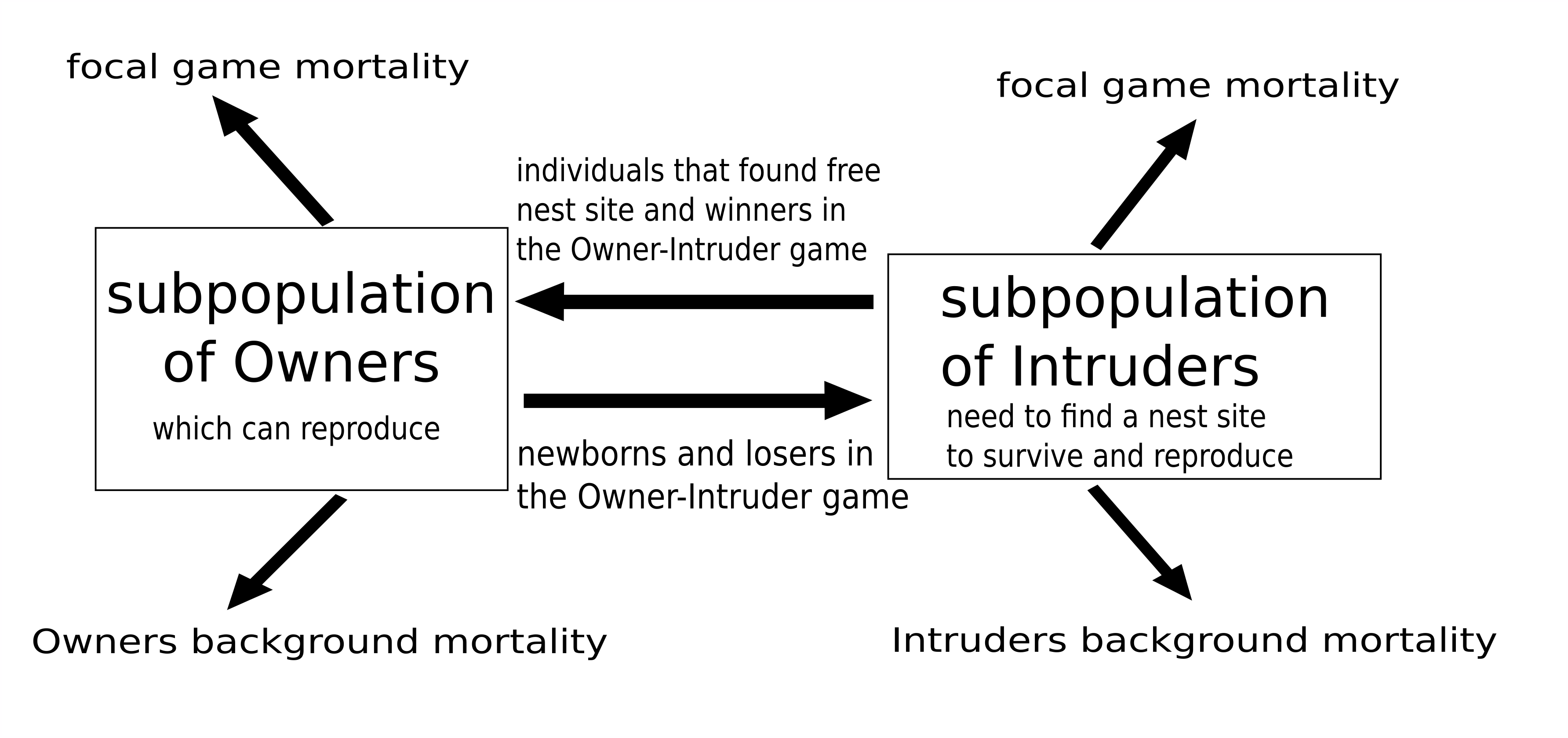
Figure 2: Structure of the model. Diagram of fluxes of indiviuals between Owner and Intruder roles and the fluxes caused by different mortality soruces.

We have two states, Owner of the Habitat and the Intruder. This leads to the two subpopulations, which strategic compositions are affected by respective mortalities and fertilities and fluxes between both roles (see Fig.2 for detailed presentation). Only Owners can reproduce and this factor will be described by their background fertility $\Phi$ and produced newborns will become homeless intruders. Intruders will randomly check the nest sites at the constant inspection rate, settle down when the nest site is free or play with the Owner. Fight for the habitat, a round of Hawk-Dove game played by Owner and Intruder, will be associated with the risk of death described by survival payoffs. The difference between basic Hawk-Dove game (Argasinski and Broom 2013,2017,2018) and a new model is that in the new model opponents are randomly drawn from separate pools (subpopulations of Owners and Intruders). This leads to different numbers of interactions per time unit (described by different interaction rates) for opposite roles (see Fig 3). By application of the concept of interaction rates (Argasinski and Broom 2017), this situation can be modelled by (15,16) and (19,22).

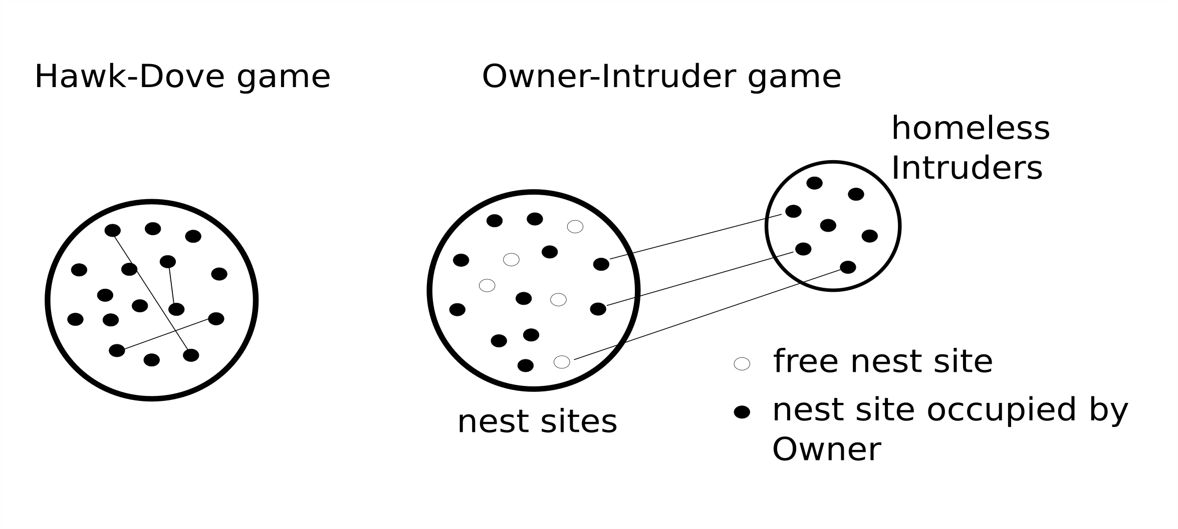
Figure 3: In Hawk-Dove game we have panmictic population with a random pair formation, thus all indiviuals will interact at the same rate. In the Owner-Intruder game Intruders check the nest-sites at the constant inspection rate. Then, for example, if we have 16 nest sites inhabited by 11 Owners and surrounded by 7 Intruders, as depicted on the figure, for three inspections per capita probability of fight for Owner is 2/11, while for Intruder 2/7. Therefore, the difference between Hawk-Dove game and Owner-Intruder game mainly depends on different interaction rates for different roles.

Behavioral patterns (actions) are Hawk (aggressive) and Dove (peaceful). Individual strategy is defined as the pair of behavioral patterns associated to the state. Thus, following the classic Maynard-Smith terminology (1982) we have Pure Hawk, Pure Dove, Bourgeois (Hawk when Owner, Dove when Intruder) and Anti-Bourgeois (opposite to Bourgeois). For each strategy the distribution of roles is described by $q_{i}^{O}=1-q_{i}^{I}$ Now we should define payoffs. Action-specific survival payoffs will be described by matrix:

$\ \ \ \ \ \ \ \ \ \begin{array}[]{cc}H&D\end{array}$
$S=\begin{array}[]{c}H\\ D\end{array}\left[\begin{array}[]{cc}s&1\\ 1&1\end{array}\right]$

and will be the same for both states. The switch payoffs will be

$\qquad\ \ \ \ \ \ \begin{array}[]{cc}H&D\end{array}$
$C^{O}=\begin{array}[]{c}H\\ D\end{array}\left[\begin{array}[]{cc}0.5&0\\ 1&0.5\end{array}\right]$     for Owners

$\qquad\ \ \ \ \ \ \ \begin{array}[]{cc}H&D\end{array}$
$C^{I}=\begin{array}[]{c}H\\ D\end{array}\left[\begin{array}[]{cc}0.5&1\\ 0&0.5\end{array}\right]$     for Intruders

Since only survivors can switch we should introduce the mortality-switching trade-off functions $Z$ (13). Thus for simplicity we should describe the model in terms of survival $s_{s}^{i}(g,q)=1-d_{s}^{i}(g,q)$. We should start the derivation of functions $Z^{O}$ and$\ Z^{I}$ by multiplying entries of $S$ and $C^{O}$ ($S$ and $C^{I}$) elementwise (the only difference will be $0.5s$ for Hawk-Hawk interaction), leading to:

$\qquad\ \ \ \ \ \ \ \ \begin{array}[]{cc}H&D\end{array}$
$Z^{O}=\begin{array}[]{c}H\\ D\end{array}\left[\begin{array}[]{cc}0.5s&0\\ 1&0.5\end{array}\right]$     for Owners

$\qquad\ \ \ \ \ \ \ \begin{array}[]{cc}H&D\end{array}$
$Z^{I}=\begin{array}[]{c}H\\ D\end{array}\left[\begin{array}[]{cc}0.5s&1\\ 0&0.5\end{array}\right]$     for Intruders

Now we should derive the arguments of those payoff functions which are distributions of actions (more specifically proportion of Hawk playing strategies among individuals of both states:

$$H^{O}=\dfrac{\sum_{H}g_{i}q_{i}^{O}}{\sum_{i}g_{i}q_{i}^{O}}\text{ \ \ and \ \ \ }H^{I}=\dfrac{\sum_{H}g_{i}q_{i}^{I}}{\sum_{i}g_{i}q_{i}^{I}}=\dfrac{\sum_{H}g_{i}\left(1-q_{i}^{O}\right)}{\sum_{i}g_{i}\left(1-q_{i}^{O}\right)}$$ (50)

(and $\sum_{H}g_{i}q_{i}^{O}$ ($\sum_{H}g_{i}q_{i}^{I}$)means sum over strategies playing Hawk as Owners (Intruders)). Proportions of Owners and Intruders will be $\sum_{i}g_{i}q_{i}^{O}$ and $1-\sum_{i}g_{i}q_{i}^{O}$. Individuals in the population compete for $K$ available nest sites (Hui 2006), then $K-n\sum_{i}g_{i}q_{i}^{O}$ will be number of free nest sites in the population. Then the Intruder will check the randomly chosen nest site and play the game with the Owner with probability

$$p_{g}=\frac{n\sum_{i}g_{i}q_{i}^{O}}{K},$$

or stay there when it is free with probability

$$1-p_{g}=\frac{K-n\sum_{i}g_{i}q_{i}^{O}}{K}.$$

Then the respective action specific survival payoffs per nest site inspection will be:

$$s_{H}^{O} = H^{I}s+(1-H^{I})=1-H^{I}\left(1-s\right),$$ (51)

$$s_{H}^{I} = \left(1-p_{g}\right)+p_{g}\left[H^{O}s+(1-H^{O})\right]$$ (52)

$$= 1-H^{O}\left(1-s\right)\frac{n\sum_{i}g_{i}q_{i}^{O}}{K},$$

$$s_{D}^{O} = s_{D}^{I}=1.$$ (53)

We have that $s_{H}^{O}$ and $s_{H}^{I}$ are always smaller than $s_{D}^{O}$ and $s_{D}^{I}$. Switching payoffs per nest site inspection will be:

$$Z_{H}^{O,I} = H^{I}0.5s+(1-H^{I})0=H^{I}0.5s$$ (54)

$$Z_{D}^{O,I} = H^{I}+(1-H^{I})0.5=0.5(1+H^{I})$$ (55)

$$Z_{H}^{,I,O} = \left(1-p_{g}\right)+p_{g}\left[H^{O}0.5s+(1-H^{O})\right]$$ (56)

$$= 1-H^{O}\left[1-0.5s\right]\frac{n\sum_{i}g_{i}q_{i}^{O}}{K}$$

$$Z_{D}^{,I,O} = \left(1-p_{g}\right)+p_{g}0.5(1-H^{O})=$$ (57)

$$= 1-\frac{n\sum_{i}g_{i}q_{i}^{O}}{K}0.5(1+H^{O})=$$

$$= 1-0.5\left(\sum_{i}g_{i}q_{i}^{O}+\sum_{H}g_{i}q_{i}^{O}\right)\frac{n}{K}$$

and always $Z_{H}^{O,I}\leq Z_{D}^{O,I}$ and $Z_{D}^{,I,O}\leq Z_{H}^{,I,O}$. In this case there are no fertility payoffs for strategies. Only Owners reproduce at the rate $\Phi$ for all strategies and their fertility feeds the Invaders subpopulation. However the reproduction is not related to the focal interaction, thus it can be regarded as background fertility $\Phi$. Then the fertility for the strategy, describing per capita growth of invaders will be

$$\Phi_{s}^{I}=\frac{q_{s}^{O}}{1-q_{s}^{O}}\Phi$$ (58)

We also assume the background mortalities for both states $\Psi_{O}<\Psi_{I}$ since Owners are safer. In addition there is no background switching, since individuals cannot leave the nest site without a reason. Above payoff functions describe survival and switching outcomes of the average interaction which is fight for the occupied nest site. However in this case, we will have different interaction rates for different states, similarly to (19,22), which means that Owners will play different number of game rounds per single time unit than Intruders (see Fig.3). Owners play the game with Intruders checking the nest sites and the probability that the nest site will be invaded is $\frac{n\left(1-\sum_{i}g_{i}q_{i}^{O}\right)}{K}$ when the number of Intruders is not greater than $K$. Otherwise, $\frac{K}{n\left(1-\sum_{i}g_{i}q_{i}^{O}\right)}$ is the probability that the Intruder will check single nest site, when the number of intruders exceeds $K$. Therefore the ratio of interaction rates is

$$\dfrac{\tau_{F}^{O}}{\tau_{F}^{I}}=\dfrac{n\left(1-\sum_{i}g_{i}q_{i}^{O}\right)}{K}$$ (59)

and it should be multiplied by Owners payoffs to obtain death and switching rates similarly to (15,16). Therefore, we can assume that the timescale of our model is adjusted to the constant Intruders inspection rate of the nest sites, however for simplicity we will limit ourselves to the cases when $n\left(1-\sum_{i}g_{i}q_{i}^{O}\right)<K$ i.e. the number of Intruders is smaller than total number of nest sites. This implies constant inspection rate for Intruders.

5.1 Switching dynamics

We can use (26), which is

$$\dot{q}_{s}^{x} = {}q_{s}^{x}\left(1-q_{s}^{x}\right)\left[\left(\Phi_{x}-\Phi_{y}\right)-\left(\Psi_{x}-\Psi_{y}\right)-\left(D_{s}^{x}(g,q)-D_{s}^{y}(g,q)\right)\right]$$ (60)

$${}+\left[\left(1-q_{s}^{x}\right)Z_{s}^{y,x}(g,q)-q_{s}^{x}Z_{s}^{x,y}(g,q)\right],$$

to describe the switching dynamics for different strategies. We can use survival payoffs (51),(52) and (53) to (15) and (16) for derivation of mortality bracket (which will be positive in equation for fraction of Owners)

$$\left(D_{s}^{I}(g,q)-D_{s}^{O}(g,q)\right)=\left(\left[1-s_{s}^{I}(g,q)\right]-\left[1-s_{s}^{O}(g,q)\right]\frac{n\left(1-\sum_{i}g_{i}q_{i}^{O}\right)}{K}\right),$$

similarly we will use switching payoffs (54), (55), (56) and (57) for derivation of the bracketed term $\left[\left(1-q_{s}^{x}\right)Z_{s}^{y,x}(g,q)-q_{s}^{x}Z_{s}^{x,y}(g,q)\right]$. Then, since $\Phi_{s}^{O}=0$ in our case and due to (58), the bracket ${}q_{s}^{x}\left(1-q_{s}^{x}\right)\left(\Phi_{x}-\Phi_{y}\right)$ reduces to negative term $\left(q_{s}^{O}\right)^{2}\Phi$. Then (60) will be

$$\dot{q}_{s}^{O} = {}q_{s}^{O}\left(1-q_{s}^{O}\right)\left[\left(\left[1-s_{s}^{I}(g,q)\right]-\left[1-s_{s}^{O}(g,q)\right]\frac{n\left(1-\sum_{i}g_{i}q_{i}^{O}\right)}{K}\right)-\left(\Psi_{O}-\Psi_{I}\right)\right]-\left(q_{s}^{O}\right)^{2}\Phi$$

$$+\left[\left(1-q_{s}^{O}\right)Z_{s}^{I,O}(g,q)-q_{s}^{O}Z_{s}^{O,I}(g,q)\frac{n\left(1-\sum_{i}g_{i}q_{i}^{O}\right)}{K}\right],$$

Thus the differences between strategies in the state switching dynamics will be described by survival and switching brackets. Note that after some rearrangement the above equation can be presented in the form revealing factors responsible for growth and decline:

$$\dot{q}_{s}^{O} = {}\left(1-q_{s}^{O}\right)\left[q_{s}^{O}\left[1-s_{s}^{I}(g,q)\right]+Z_{s}^{I,O}(g,q)\right]-q_{s}^{O}\left[{}\left(1-q_{s}^{O}\right)\left[1-s_{s}^{O}(g,q)\right]+Z_{s}^{O,I}(g,q)\right]\frac{n\left(1-\sum_{i}g_{i}q_{i}^{O}\right)}{K}$$ (61)

$$-{}q_{s}^{O}\left(1-q_{s}^{O}\right)\left(\Psi_{O}-\Psi_{I}\right)-\left(q_{s}^{O}\right)^{2}\Phi{},$$

showing that for growth is responsible action chosen as Intruder and its impact is described by the term $\mathbf{Inc}=\left(q_{s}^{O}\left[1-s_{s}^{I}(g,q)\right]+Z_{s}^{I,O}(g,q)\right)$, while decline is determined by action chosen as Owner and its impact is described by term $\mathbf{Dec}=\left(\left(1-q_{s}^{O}\right)\left[1-s_{s}^{O}(g,q)\right]+Z_{s}^{O,I}(g,q)\right)$. Then the switching dynamics (61) can be denoted in the simplified form:

$$\dot{q}_{s}^{O}={}\left(1-q_{s}^{O}\right)\mathbf{Inc}-q_{s}^{O}\mathbf{Dec}\frac{n\left(1-\sum_{i}g_{i}q_{i}^{O}\right)}{K}-{}q_{s}^{O}\left(1-q_{s}^{O}\right)\left(\Psi_{O}-\Psi_{I}\right)-\left(q_{s}^{O}\right)^{2}\Phi.$$ (62)

Now we can derive the increase and decrease factors for Hawk and Dove actions:

$$\mathbf{Inc}_{H} = q_{s}^{O}H^{O}\left(1-s\right)\frac{n\sum_{i}g_{i}q_{i}^{O}}{K}+1-H^{O}\left[1-0.5s\right]\frac{n\sum_{i}g_{i}q_{i}^{O}}{K}$$

$$= 1+\left[q_{s}^{O}\left(1-s\right)-1+0.5s\right]H^{O}\frac{n\sum_{i}g_{i}q_{i}^{O}}{K}$$

$$\mathbf{Inc}_{D} = 1-(1+H^{O})0.5\frac{n\sum_{i}g_{i}q_{i}^{O}}{K}$$

$$\mathbf{Dec}_{H} = \left[\left(1-q_{s}^{O}\right)\left(1-s\right)+0.5s\right]H^{I}$$

$$\mathbf{Dec}_{D} = 0.5(1+H^{I}).$$

Note that $\mathbf{Inc}_{D}>\mathbf{Inc}_{H}$ when

$$(1+H^{O})0.5 < \left[1-q_{s}^{O}\left(1-s\right)-0.5s\right]H^{O}$$

$$0.5 < \left(0.5-q_{s}^{O}\right)(1-s)H^{O}.$$

This condition is never satisfied. Similarly we have that $\mathbf{Dec}_{D}>\mathbf{Dec}_{H}$ when

$$(1+H^{I})0.5 > \left[\left(1-q_{s}^{O}\right)\left(1-s\right)+0.5s\right]H^{I}$$

$$0.5 > \left(0.5-q_{s}^{O}\right)\left(1-s\right)H^{I}.$$

The second condition is always satisfied except the marginal case of $q_{s}^{O}=s=0$ and $H^{I}=1$. In effect Hawk action is most efficient for switching in both roles. By substituting increase and decrease factors to (62) we can derive switching dynamics for respective strategies:
Hawk strategy ($\mathbf{Inc}_{H}$ and $\mathbf{Dec}_{H}$)

$$\dot{q}_{H}^{O} = {}\left(1-q_{H}^{O}\right)\left(1+\left[q_{H}^{O}\left(1-s\right)-1+0.5s\right]H^{O}\frac{n\sum_{i}g_{i}q_{i}^{O}}{K}\right)$$

$$-q_{H}^{O}\left[\left(1-q_{H}^{O}\right)\left(1-s\right)+0.5s\right]H^{I}\frac{n\left(1-\sum_{i}g_{i}q_{i}^{O}\right)}{K}$$

$$-{}q_{H}^{O}\left(1-q_{H}^{O}\right)\left(\Psi_{O}-\Psi_{I}\right)-\left(q_{H}^{O}\right)^{2}\Phi$$

Dove strategy ($\mathbf{Inc}_{D}$ and $\mathbf{Dec}_{D}$)

$$\dot{q}_{D}^{O} = {}\left(1-q_{D}^{O}\right)\left(1-(1+H^{O})0.5\frac{n\sum_{i}g_{i}q_{i}^{O}}{K}\right)-q_{D}^{O}0.5(1+H^{I})\frac{n\left(1-\sum_{i}g_{i}q_{i}^{O}\right)}{K}$$

$$-{}q_{D}^{O}\left(1-q_{D}^{O}\right)\left(\Psi_{O}-\Psi_{I}\right)-\left(q_{D}^{O}\right)^{2}\Phi.$$

Bourgeois strategy ($\mathbf{Inc}_{D}$ and $\mathbf{Dec}_{H}$)

$$\dot{q}_{B}^{O} = {}\left(1-q_{B}^{O}\right)\left(1-(1+H^{O})0.5\frac{n\sum_{i}g_{i}q_{i}^{O}}{K}\right)-q_{B}^{O}\left[\left(1-q_{B}^{O}\right)\left(1-s\right)+0.5s\right]H^{I}\frac{n\left(1-\sum_{i}g_{i}q_{i}^{O}\right)}{K}$$

$$-{}q_{B}^{O}\left(1-q_{B}^{O}\right)\left(\Psi_{O}-\Psi_{I}\right)-\left(q_{B}^{O}\right)^{2}\Phi.$$

Antibourgeois strategy ($\mathbf{Inc}_{H}$ and $\mathbf{Dec}_{D}$)

$$\dot{q}_{A}^{O} = {}\left(1-q_{A}^{O}\right)\left(1+\left[q_{A}^{O}\left(1-s\right)-1+0.5s\right]H^{O}\frac{n\sum_{i}g_{i}q_{i}^{O}}{K}\right)-q_{A}^{O}0.5(1+H^{I})\frac{n\left(1-\sum_{i}g_{i}q_{i}^{O}\right)}{K}$$

$$-{}q_{A}^{O}\left(1-q_{A}^{O}\right)\left(\Psi_{O}-\Psi_{I}\right)-\left(q_{A}^{O}\right)^{2}\Phi.$$

5.2 Mortality stage

Average mortality rates are:

$$\bar{D}_{H}(g,q,n)=\left[q_{H}^{O}H^{I}\left(1-\sum_{i}g_{i}q_{i}^{O}\right)+\left(1-q_{H}^{O}\right)H^{O}\sum_{i}g_{i}q_{i}^{O}\right]\frac{n}{K}(1-s)$$

$$\bar{D}_{D}(g,q,n)=0$$

$$\bar{D}_{B}(g,q,n)=q_{B}^{O}H^{I}\left(1-s\right)\frac{n\left(1-\sum_{i}g_{i}q_{i}^{O}\right)}{K}$$

$$\bar{D}_{A}(g,q,n)=\left(1-q_{A}^{O}\right)H^{O}\left(1-s\right)\frac{n\sum_{i}g_{i}q_{i}^{O}}{K}.$$

where $\bar{D}_{D}$ is smallest and $\bar{D}_{H}$ greatest, and $\bar{D}_{B}<\bar{D}_{A}$ when

$$\frac{q_{B}^{O}}{\sum_{H}g_{i}q_{i}^{O}}<\frac{\left(1-q_{A}^{O}\right)}{\sum_{H}g_{i}\left(1-q_{i}^{O}\right)}$$

Average mortality rate of the whole population is:

$$\bar{D}(g,q,n)=g_{H}\bar{D}_{H}(g,q,n)+g_{D}\bar{D}_{D}(g,q,n)+g_{B}\bar{D}_{B}(g,q,n)+g_{A}\bar{D}_{A}(g,q,n)$$

$$=\left[\left(g_{H}q_{H}^{O}+g_{B}q_{B}^{O}\right)H^{I}\left(1-s\right)\left(1-\sum_{i}g_{i}q_{i}^{O}\right)+\left(g_{H}\left(1-q_{H}^{O}\right)+g_{A}\left(1-q_{A}^{O}\right)\right)H^{O}\left(1-s\right)\sum_{i}g_{i}q_{i}^{O}\right]\frac{n}{K}.$$ (63)

Detailed derivation is in Appendix 1

5.3 Selection dynamics

Now let us describe the selection dynamics

$$\dot{g}_{s}=g_{s}\left[\left(\bar{\Phi}_{s}(q_{s}^{O})-\bar{\Phi}(g,q)\right)-\left(\bar{D}_{s}(g,q,n)-\bar{D}(g,q,n)\right)-\left(\bar{\Psi}_{s}(q_{s})-\bar{\Psi}(g,q)\right)\right],$$ (64)

which can be reduced to

$$\dot{g}_{s}=g_{s}\left[\left[\Phi-\Psi_{O}+\Psi_{I}\right]\left(q_{s}^{O}-\sum_{i}gq_{i}^{O}\right)-\left(\bar{D}_{s}(g,q,n)-\bar{D}(g,q,n)\right)\right].$$ (65)

Detailed derivation is in Appendix 2.
The equation for population size will be:

$$\dot{n} = n\left[\bar{\Phi}(g,q)-\bar{\Psi}(g,q)-\bar{D}(g,q,n)\right]$$

$$= n\left[\left[\Phi-\Psi_{O}+\Psi_{I}\right]\sum_{i}g_{i}q_{i}^{O}-\Psi_{I}-\bar{D}(g,q,n)\right].$$

Impact of the population size $n$ on function $\bar{D}(g,q,n)$ is realized by multiplicative term $\dfrac{n}{K}$. Therefore, the average mortality (63) can be presented as $\bar{D}(g,q,n)=\tilde{D}(g,q)\dfrac{n}{K}$, in effect attractor population size can be calculated:

$$\tilde{n}=K\frac{\left[\Phi-\Psi_{O}+\Psi_{I}\right]\sum_{i}g_{i}q_{i}^{O}-\Psi_{I}}{\tilde{D}(g,q)}$$

Therefore (65) contains two factors, first term $\left(q_{s}^{O}-\sum_{i}gq_{i}^{O}\right)$ weighted by background payoffs bracket describes differences in role distributions of the subpopulations of carriers, and the second term $\left(\bar{D}_{s}(g,q,n)-\bar{D}(g,q,n)\right)$ describes differences in average mortalities resulting from role distributions too, but also from individual actions determined by strategies. Thus it mixes the results of strategies used in the focal interaction and background payoffs. In addition level of individual interactions is determined by actual compositions of the carrier subpopulations and we have complex trade-offs between those levels. This is even more complicated situation than in the case of the sex ratio evolution (Argasinski 2012, 2013, 2018) where selection is determined by sex ratios in carrier subpopulations (thus subpopulation compositions not individual traits) while individual actions are responsible for the adjustment of those sex ratios leading to the double level selection system. However, the difference between those systems is that in the case of sex ratio evolution adjustment of the subpopulation composition is realized by demographic process (differences in the numbers of births) while in Owner-Intruder game by switching dynamics independent from demography. Therefore, it cannot be regarded as the multi-level selection, even if the subpopulation composition plays important role in this process. This is rather related to the extended phenotype concept (Dawkins 2016), since the subpopulation composition is the direct result of the behaviour (i.e. leaving the property or not).

5.4 Obtained system

Summarizing the above derivations we have the system

$$\dot{q}_{H}^{O} = {}\left(1-q_{H}^{O}\right)\left(1+\left[q_{H}^{O}\left(1-s\right)-1+0.5s\right]H^{O}\frac{n\sum_{i}g_{i}q_{i}^{O}}{K}\right)$$ (66)

$$-q_{H}^{O}\left[\left(1-q_{H}^{O}\right)\left(1-s\right)+0.5s\right]H^{I}\frac{n\left(1-\sum_{i}g_{i}q_{i}^{O}\right)}{K}$$

$$-{}q_{H}^{O}\left(1-q_{H}^{O}\right)\left(\Psi_{O}-\Psi_{I}\right)-\left(q_{H}^{O}\right)^{2}\Phi$$

$$\dot{q}_{D}^{O} = {}\left(1-q_{D}^{O}\right)\left(1-(1+H^{O})0.5\frac{n\sum_{i}g_{i}q_{i}^{O}}{K}\right)-q_{D}^{O}0.5(1+H^{I})\frac{n\left(1-\sum_{i}g_{i}q_{i}^{O}\right)}{K}$$ (67)

$$-{}q_{D}^{O}\left(1-q_{D}^{O}\right)\left(\Psi_{O}-\Psi_{I}\right)-\left(q_{D}^{O}\right)^{2}\Phi.$$

$$\dot{q}_{B}^{O} = {}\left(1-q_{B}^{O}\right)\left(1-(1+H^{O})0.5\frac{n\sum_{i}g_{i}q_{i}^{O}}{K}\right)-q_{B}^{O}\left[\left(1-q_{B}^{O}\right)\left(1-s\right)+0.5s\right]H^{I}\frac{n\left(1-\sum_{i}g_{i}q_{i}^{O}\right)}{K}$$ (68)

$$-{}q_{B}^{O}\left(1-q_{B}^{O}\right)\left(\Psi_{O}-\Psi_{I}\right)-\left(q_{B}^{O}\right)^{2}\Phi.$$

$$\dot{q}_{A}^{O} = {}\left(1-q_{A}^{O}\right)\left(1+\left[q_{A}^{O}\left(1-s\right)-1+0.5s\right]H^{O}\frac{n\sum_{i}g_{i}q_{i}^{O}}{K}\right)-q_{A}^{O}0.5(1+H^{I})\frac{n\left(1-\sum_{i}g_{i}q_{i}^{O}\right)}{K}$$ (69)

$$-{}q_{A}^{O}\left(1-q_{A}^{O}\right)\left(\Psi_{O}-\Psi_{I}\right)-\left(q_{A}^{O}\right)^{2}\Phi.$$

$$\dot{g}_{D}=g_{D}\left[\left[\Phi-\Psi_{O}+\Psi_{I}\right]\left(q_{D}^{O}-\sum_{i}g_{i}q_{i}^{O}\right)+\tilde{D}(g,q)\dfrac{n}{K}\right]$$ (70)

$$\dot{g}_{B}=g_{B}\left[\left[\Phi-\Psi_{O}+\Psi_{I}\right]\left(q_{B}^{O}-\sum_{i}g_{i}q_{i}^{O}\right)-\left(q_{B}^{O}H^{I}\left(1-s\right)\frac{n\left(1-\sum_{i}g_{i}q_{i}^{O}\right)}{K}-\tilde{D}(g,q)\dfrac{n}{K}\right)\right]$$ (71)

$$\dot{g}_{A}=g_{A}\left[\left[\Phi-\Psi_{O}+\Psi_{I}\right]\left(q_{A}^{O}-\sum_{i}g_{i}q_{i}^{O}\right)-\left(\left(1-q_{A}^{O}\right)H^{O}\left(1-s\right)\frac{n\sum_{i}g_{i}q_{i}^{O}}{K}-\tilde{D}(g,q)\dfrac{n}{K}\right)\right]$$ (72)

$$\dot{n} = n\left[\bar{\Phi}(g,q)-\bar{\Psi}(g,q)-\bar{D}(g,q)\right]$$ (73)

$$= n\left[\left[\Phi-\Psi_{O}+\Psi_{I}\right]\sum_{i}g_{i}q_{i}^{O}-\Psi_{I}-\tilde{D}(g,q)\dfrac{n}{K}\right]$$

where

$$\tilde{D}(g,q) = \left[\left(g_{H}q_{H}^{O}+g_{B}q_{B}^{O}\right)H^{I}\left(1-s\right)\left(1-\sum_{i}g_{i}q_{i}^{O}\right)+\left(g_{H}\left(1-q_{H}^{O}\right)+g_{A}\left(1-q_{A}^{O}\right)\right)H^{O}\left(1-s\right)\sum_{i}g_{i}q_{i}^{O}\right]$$

$$H^{O} = \dfrac{\sum_{H}g_{i}q_{i}^{O}}{\sum_{i}g_{i}q_{i}^{O}}\text{ \ \ and \ \ \ }H^{I}=\dfrac{\sum_{H}g_{i}\left(1-q_{i}^{O}\right)}{\sum_{i}g_{i}\left(1-q_{i}^{O}\right)},$$

and the attracting density surface is:

$$\tilde{n}=K\frac{\left[\Phi-\Psi_{O}+\Psi_{I}\right]\sum_{i}g_{i}q_{i}^{O}-\Psi_{I}}{\tilde{D}(g,q)}$$

5.5 Resulting static fitness measure

From selection dynamics (65) we can derive proper static fitness function which is

$$F_{s}(g,q)=q_{s}^{O}\left[\Phi-\Psi_{O}+\Psi_{I}\right]-\bar{D}_{s}(g,q,n).$$

Therefore selection is driven by two factors, focal interaction average mortality $\bar{D}_{s}(g,q,n)$ and the differences in background vital rates caused by different role allocations. The second stage is described by factor $q_{s}^{O}\left[\Phi-\Psi_{O}+\Psi_{I}\right]$. Note that role allocation affects the value of $\bar{D}_{s}(g,q,n)$ too. In the expanded form above function can be presented as

$$F_{s}(g,q)=q_{s}^{O}\left(\Phi-\Psi_{O}+\Psi_{I}\right)-\left(q_{s}^{O}\left[1-s_{s}^{O}(g,q)\right]\frac{n\left(1-\sum_{i}g_{i}q_{i}^{O}\right)}{K}+\left(1-q_{s}^{O}\right)\left[1-s_{s}^{I}(g,q)\right]\right)$$

substitution of the respective action specific survival payoffs (51), (52) and (53) for $s_{s}^{O}(g,q)$ and $s_{s}^{I}(g,q)$ leads to

$$F_{H}(g,q) = q_{H}^{O}\left(\Phi-\Psi_{O}+\Psi_{I}\right)-\left[q_{H}^{O}H^{I}\left(1-\sum_{i}g_{i}q_{i}^{O}\right)+\left(1-q_{H}^{O}\right)H^{O}\sum_{i}g_{i}q_{i}^{O}\right]\frac{n}{K}\left(1-s\right)$$

$$F_{D}(g,q) = q_{D}^{O}\left(\Phi-\Psi_{O}+\Psi_{I}\right)$$

$$F_{B}(g,q) = q_{B}^{O}\left(\Phi-\Psi_{O}+\Psi_{I}\right)-q_{B}^{O}\left(1-\sum_{i}g_{i}q_{i}^{O}\right)H^{I}\frac{n}{K}\left(1-s\right)$$

$$F_{A}(g,q) = q_{A}^{O}\left(\Phi-\Psi_{O}+\Psi_{I}\right)-\left(1-q_{s}^{O}\right)\sum_{i}g_{i}q_{i}^{O}H^{O}\frac{n}{K}\left(1-s\right)$$

6 Numerical simulations

Due to complexity of the obtained model, to avoid the inflation of the paper, we will limit ourselves to numerical simulations, leaving the detailed analysis for the separate paper. First important thing is the choice of the biologically relevant values of parameters. Let us focus on the background mortality and fertility rates $\Psi_{O}$, $\Psi_{I}$ and $\Phi$. The timescale of the model is adjusted to the constant Intruder’s per capita intensity of nest site inspection (equivalent to the interaction rate with possible Owner) which leads to (59). Therefore, realistic situation is when Owners background mortality $\Psi_{O}$ is significantly smaller than respective parameter for Intruders $\Psi_{I}$. Fertility rate $\Phi$ should be greater than average mortality to avoid the extinction of the population. Inspections of the nest sites occur in the behavioral timescale and are more frequent than births and background deaths. This will allow Intruders to do few inspections before death. Therefore, background vital rates should be smaller than focal game interaction rate, leading to $\Psi_{O}<\Psi_{I}<\Phi<1$. In those cases new model reproduces the predictions that are known from literature. Competition between pure Hawk and pure Dove leads to the mixed equilibrium which depends on the survival of the fight between Hawks. This situation is shown on Fig.4, for very low fight survival probability $s=0,001$ and the background mortality and fertility rates $\Psi_{O}=0.01$, $\Psi_{I}=0.2$ and $\Phi=0.05$. What is interesting, for such harsh conditions the stable frequency of hawks is relatively high, in addition the proportion of Owners among Hawks is close to 1, while for Doves is slightly lower. In effect subpopulation of homeless Intruders contains majority of Doves. Another interesting observation is that the total population size is smaller than the number of nest sites $K$. Therefore, in the environment is enough nest sites for all individuals. This means that the availability of nest sites is not the main limiting factor here. The suppression is driven by pressure of the background mortality related to the searching for free nest site. Simulations also show that both pure strategies are outcompeted by Bourgeois and paradoxical Antibourgeois strategies. Both those strategies can successfully invade the population and be evolutionarily stable. In the population composed of competing Bourgeois and Antibourgeois individuals, both strategies are stable and invasion barrier is exactly 0.5. However, when we add some fraction of Hawks or Doves, the invasion barrier will shift closer to the Antibourgeois pure state, leading to the increase of the basin of attraction of Bourgeois. For some parameter values it is possible another interesting situation, when Bourgeois is not stable but exists mixed equilibrium composed of Bourgeois and small fraction of pure Hawks. Let us focus on this situation. Assume that number of nest sites is $K=10000$. We can choose values $\Psi_{O}=0.01$, $\Psi_{I}=0.2$ and $\Phi=0.8$ and the survival of the fight as $s=0.4$. For initial state of the population we assume that $n(0)=70$ and all for all strategies role distributions are equal to $0.1$ and gene frequencies to $0.25$. The trajectories of population parameters are depicted on Fig.5. In addition, Fig.6 shows changes in the average mortalities $\bar{D}_{s}(g,q,n)$ for all strategies and frequencies of Hawks among Owners and Intruders $H^{O}$ and $H^{I}$, which determine those mortalities. They show the increase in mortality associated with population growth. This is caused by increasing number of fights related to the increase of the fraction of the occupied nest sites.

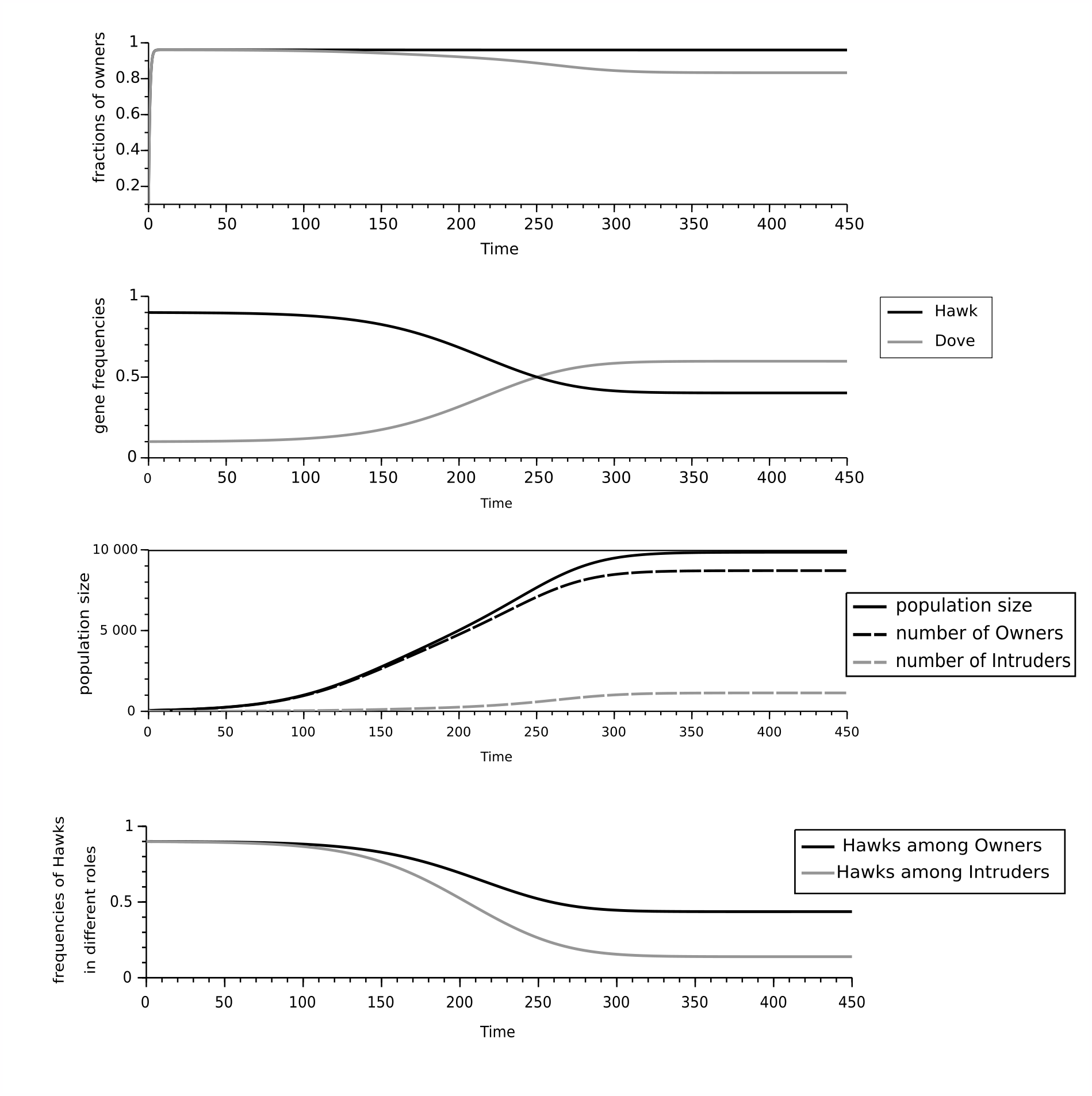
Figure 4: Case of competing pure Hawk and Dove strategies. Plots of role distributions $q_{s}^{O}$, strategy frequencies $g_{s}$ and numbers of Owners $n\sum_{s}g_{s}q_{s}^{O}$, Intruders $n\left(1-\sum_{s}g_{s}q_{s}^{O}\right)$ and the population size $n$. Last panel shows proportions of Hawks among Owners and Intruders. Proportion of Owners among Hawks is close to 1 while among doves is sligtly lower. On the other hand among Intruders we have majority of Doves. In effect among reproducing Owners thie proportion of Hawks is slightly greater than Hawk gene frequency. Interesting is that the stable population sizeis lower than the number of nest sites, thus this is not a lomiting factor in this case. Suppression is rather driven by background mortalities.

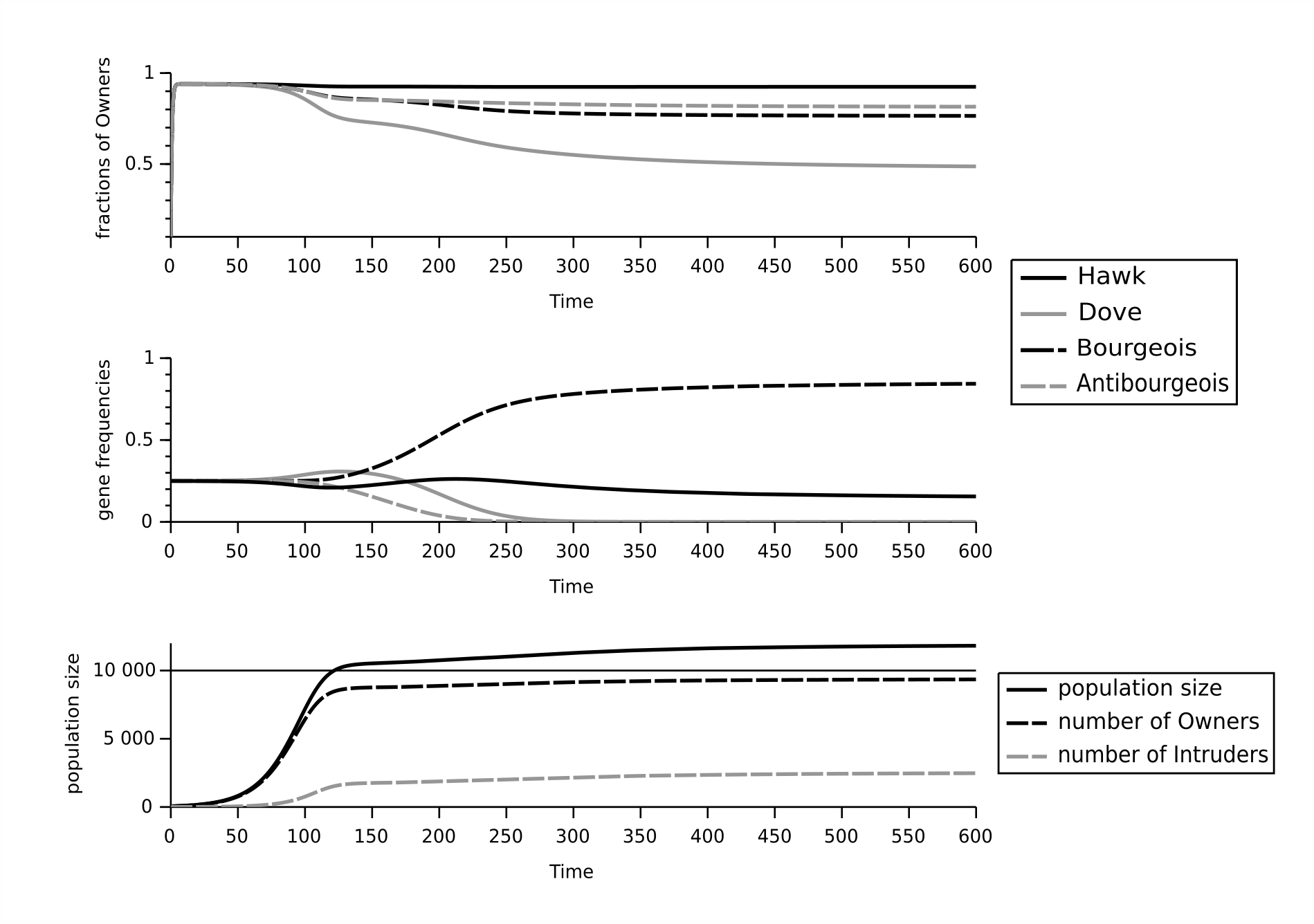
Figure 5: Plots of role distributions $q_{s}^{O}$, strategy frequencies $g_{s}$ and numbers of Owners $n\sum_{s}g_{s}q_{s}^{O}$, Intruders $n\left(1-\sum_{s}g_{s}q_{s}^{O}\right)$ and the population size $n$. Interesting is that the system converged to the mixture of Bourgeois and pure Hawks

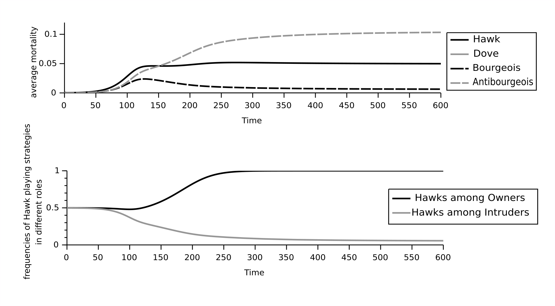
Figure 6: Plots of changes in average mortality rates $\bar{D}_{s}$ for all strategies and frequencies of Hawk playing strategies among Owners and Intruders $H^{O}$ and $H^{I}$. Note that mortality increases with the population growth since fights become more frequent.

7 Discussion

In this paper we introduced the combination of the dynamic evolutionary games with the state based approach. We presented the system of differential equations which describes the dynamics of state changes and completes the replicator dynamics. Our new framework can be useful in the integration of many distinct fields of theoretical evolutionary biology into coherent synthetic theory. We illustrated this by examples of application of the new framework to the classical problems.

The natural processes such as aging or the developmental process can be described in terms of state changing processes. It can be useful for formalization of the game theoretic notions such as ”costs” and ”benefits” in terms of the stages of a life cycle of the individual. We presented a simple attempt to this problem which shows the complexity of the phenomenon. This example shows that the new framework presented in this paper can be used in life history modelling (Stearns 1992, Roff 2002) The future research on this topic should investigate the relationships of this type of models with results related to the classical demography.

Example of dynamic owner-intruder game shows the complexity of the process underlying the changes of life situation determined by strategy. It clearly shows that the assumption in the classical models (Maynard Smith 1982) that the individual can be owner or intruder with the probability 0.5 was very strong simplification. Owner-Intruder example emphasizes the importance of the definition of the demographic vital rates as the products of the interaction rates and the demographic outcomes of the interaction (interpreted as the game round, Argasinski and Broom 2018a). In this example different interaction rates for opposite roles should be explicitly considered in the model (for example in the average mortalities) thus this problem cannot be clearly described in terms of abstract fitnesses expressed in units of instantaneous growth rates. The case of stable mixed Bourgeois/Hawk state is important from the point of view of the latest theories on the impact of density dependence on the selection mechanisms, which are one of important questions (Dańko et al 2018). Latest Nest Site Lottery models (Argasinski and Broom 2013b, Argasinski and Rudnicki 2017, Rudnicki 2018, Argasinski and Rudnicki submitted) silently assume that all newborns competing for free nest sites are Bourgeois. Our new model shows that this may be not the case. Some newborns can be Hawks and can try to attack the occupied nest sites. Presence of small but significant fraction of Hawks may alter the selection mechanism. Note that our model describes very specific conflict for supply which are nest sites. Conflict for other supplies such as food will have different structure and will be driven by different mechanisms, for example models of kleptoparasitism describe situations when ownership is not respected (Broom and Ruxton 1998; Broom and Rychtar 2007,2009,2011; Luther et al 2007; Broom et al 2009) This suggests that there is no general explanation for ownership respect and different forms of ownership are shaped by different selection mechanisms. Therefore we can expect different behavioral patterns for those distinct conflicts, which means that the respect for nest site may not imply respect for ownership of food and vice versa.

Important reason shown by new approach is the importance of the state distribution for the determination of fitness, which is the quantity related to the population growth rate (Metz 2008) but can be formalized in many ways (Roff 2009). The dynamic equilibria of the state changing process, constituting the role/state distributions, should be explicitly taken into consideration in the fitness evaluation. The possible perturbations of the stable distribution of states should be incorporated to the modern development of the ESS theory to increase its consistence (Houston and McNamara 2005, McNamara 2013) . This will be interesting contribution to theoretical studies related to the individual level, originated by Łomnicki (1988), and in particular related to research on animal personalities (Dall et al. 2004; Wolf et al. 2007; Wolf and Weissing 2010, Wolf and Weissing 2012; Wolf and McNamara 2012).

We want to thank John McNamara for scientific mentoring, helpful suggestions and support during scientific visits. In addition, we want to thank Mark Broom and Jan Kozłowski a for their support of the project. This paper was supported by the Polish National Science Centre Grant No. 2013/08/S/NZ8/00821 FUGA2 (KA) and Grant No. 2017/27/B/ST1/00100 OPUS (RR)

References

Argasinski K. (2006) Dynamic multipopulation and density dependent evolutionary games related to replicator dynamics. A metasimplex concept. Math Biosci 202 88-114.
Argasinski K. (2012) The dynamics of sex ratio evolution Dynamics of global population parameters. J Theor Biol 309 134-146.
Argasinski K. (2013) The Dynamics of Sex Ratio Evolution: From the Gene Perspective to Multilevel Selection. PloS ONE, 8(4), e60405
Argasinski K. (2018) The dynamics of sex ratio evolution: the impact of males as passive gene carriers on multilevel selection. Dynamic Games and Applications, 8(4), 671-695.
Argasinski K. Broom M. (2013a) Ecological theatre and the evolutionary game: how environmental and demographic factors determine payoffs in evolutionary games. J Math Biol. 1;67(4):935-62.
Argasinski K. Broom M.(2013b) The nest site lottery: how selectively neutral density dependent growth suppression induces frequency dependent selection. Theor Pop Biol 90 82-90.
Argasinski, K. Broom M. (2018a). Interaction rates, vital rates, background fitness and replicator dynamics: how to embed evolutionary game structure into realistic population dynamics. Theory in Biosciences, 137(1), 33-50.
Argasinski K. Broom M. (2018b). Evolutionary stability under limited population growth: Eco-evolutionary feedbacks and replicator dynamics. Ecological Complexity, 34, 198-212.
Argasinski K, Rudnicki R. (2017). Nest site lottery revisited: Towards a mechanistic model of population growth suppressed by the availability of nest sites. J Theor Biol, 420, 279-289.
Cressman R. (1992) The Stability Concept of Evolutionary Game Theory. Springer.
Cressman R., & Křivan, V. (2019). Bimatrix games that include interaction times alter the evolutionary outcome: The Owner–Intruder game. Journal of theoretical biology, 460, 262-273.
Dańko MJ, Burger O, Argasiński K, & Kozłowski, J (2018). Extrinsic mortality can shape life-history traits, including senescence. Evolutionary biology, 45(4), 395-404.
Broom M., Ruxton G. D. (1998). Evolutionarily stable stealing: game theory applied to kleptoparasitism. Annals of Human Genetics, 62(5), 453-464.
Broom, M., Rychtář, J. (2007). The evolution of a kleptoparasitic system under adaptive dynamics. Journal of Mathematical Biology, 54(2), 151-177.
Broom, M., Rychtář, J. (2009). A game theoretical model of kleptoparasitism with incomplete information. Journal of mathematical biology, 59(5), 631-649.
Broom, M., Luther, R. M., Rychtár, J. (2009). A hawk-dove game in kleptoparasitic populations. Journal of Combinatorics, Information and System Sciences, 4, 449-462.
Broom, M., Rychtář, J. (2011). Kleptoparasitic melees—modelling food stealing featuring contests with multiple individuals. Bulletin of mathematical biology, 73(3), 683-699.
Brunetti, I., Hayel, Y., & Altman, E. (2015). State policy couple dynamics in evolutionary games. In 2015 American Control Conference (ACC) (pp. 1758-1763). IEEE.
Brunetti, I., Hayel, Y., & Altman, E. (2018). State-policy dynamics in evolutionary games. Dynamic Games and Applications, 8(1), 93-116.
Dawkins R (2016).The extended phenotype: The long reach of the gene. Oxford University Press.
Eshel I, Sansone E. (1995). Owner-intruder conflict, Grafen effect and self-assessment. The bourgeois principle re-examined. J. Theor Biol, 177(4), 341-356.
Grafen A. (2006) Optimization of inclusive fitness. Journal of Theoretical Biology. Feb 7;238(3):541-63.
Grafen A. (1987). The logic of divisively asymmetric contests: respect for ownership and the desperado effect. Anim. Behav. 35, 462–467.
Hofbauer J, Sigmund.K (1988) The Theory of Evolution and Dynamical Systems. Cambridge University Press.
Hofbauer J, Sigmund.K (1998) Evolutionary Games and Population Dynamics. Cambridge University Press.
Houston AI, McNamara J (1999) JM. Models of adaptive behaviour: an approach based on state. Cambridge University Press;
Houston AI, McNamara J (2005). John Maynard Smith and the importance of consistency in evolutionary game theory. Biol Phil 20(5) 933-950.
Huang W, Hauert C, Traulsen A (2015). Stochastic game dynamics under demographic fluctuations. PNAS, 112(29), 9064-9069
Hui, C. (2006). Carrying capacity, population equilibrium, and environment’s maximal load. Ecological Modelling, 192(1-2), 317-320.
Hauert C, Holmes M. Doebeli M (2006) Evolutionary games and population dynamics: maintenance of cooperation in public goods games. Proceedings of the Royal Society B: Biological Sciences, 273(1600), pp.2565–2570.
Hauert C, Wakano JY, Doebeli M, (2008) Ecological public goods games: cooperation and bifurcation. Theor Pop Biol, 73(2), pp.257–263
Leimar, O., & Enquist, M. (1984). Effects of asymmetries in owner-intruder conflicts. Journal of theoretical Biology, 111(3), 475-491.
Kokko H, López-Sepulcre, A Morrell LJ (2006). From hawks and doves to self-consistent games of territorial behavior. The American Naturalist, 167(6), 901-912
Kokko H, (2013) Dyadic contests: Modelling figths between two individuals, in: Animal contests Hardy, I. C., & Briffa, M. (Eds.) Cambridge University Press
Korona, R. (1989). Evolutionarily stable strategies in competition for resource intake rate maximization. Behavioral ecology and sociobiology, 25(3), 193-199
Korona, R. (1991). On the role of age and body size in risky animal contests. Journal of theoretical biology, 152(2), 165-176
Křivan V, Galanthay TE, & Cressman R. (2018). Beyond replicator dynamics: From frequency to density dependent models of evolutionary games. J. Theor. Biol. , 455, 232-248.
Luther, R. M., Broom, M., & Ruxton, G. D. (2007). Is food worth fighting for? ESS’s in mixed populations of kleptoparasites and foragers. Bulletin of mathematical biology, 69(4), 1121-1146.
Łomnicki A (1988). Population ecology of individuals. Princeton University Press, Princeton, New Jersey.
Maynard Smith J (1982) Evolution and the Theory of Games. Cambridge University Press, Cambbridge, United Kingdom.
McElreath, R., & Boyd, R. (2008). Mathematical models of social evolution: A guide for the perplexed. University of Chicago Press.
McNamara JM (2013). Towards a richer evolutionary game theory. J Roy Soc Interface 10(88) 20130544.
Mylius, S. D. (1999). What pair formation can do to the battle of the sexes: towards more realistic game dynamics. J. Theor. Biol, 197(4), 469-485.
Roff DA (2008). Defining fitness in evolutionary models. J Genet 87, 339–348.
Roff DA (2002) Life history evolution. Sinauer
Rudnicki R (2017). Does a population with the highest turnover coefficient win competition?. Journal of Difference Equations and Applications, 23(9), 1529-1541.
Sherratt TN, Mesterton-Gibbons M. (2015). The evolution of respect for property. Journal of evolutionary biology, 28(6), 1185-1202.
Stearns SC.(1992) The evolution of life histories. Oxford: Oxford University Press
Metz JAJ (2008). Fitness. In: Jørgensen, S.E., Fath, B.D. (Eds.), Evolutionary Ecology. In: Encyclopedia of Ecology, vol. 2. Elsevier, pp. 1599–1612.
Taylor PD. (1996) Inclusive fitness arguments in genetic models of behaviour. Journal of mathematical biology. May 1;34(5-6):654-74.
Van Veelen M. (2009) Group selection, kin selection, altruism and cooperation: when inclusive fitness is right and when it can be wrong. Journal of Theoretical Biology. Aug 7;259(3):589-600
Wolf M., McNamara JM. (2012). On the evolution of personalities via frequency-dependent selection. Am Nat 179(6), 679-692.
Wolf M, Van Doorn GS, Leimar O, Weissing FJ. (2007). Life-history trade-offs favour the evolution of animal personalities. Nature, 447(7144), 581-584.
Wolf M, Weissing FJ. (2010). An explanatory framework for adaptive personality differences. Phil Trans Proc Roy Soc B 365(1560), 3959-3968.
Wolf M, Weissing FJ. (2012). Animal personalities: consequences for ecology and evolution. Trends Ecol Evol 27(8), 452-461.
Zhang F, Hui C (2011) Eco-Evolutionary Feedback and the Invasion of Cooperation in Prisoner’s Dilemma Games. PLoS ONE 6(11) e27523.
doi:10.1371/journal.pone.0027523

Appendix 1 Derivation of mortality rates

Average mortality rates for respective strategies are

$$\bar{D}_{H}(g,q,n) = q_{H}^{O}\left[1-s_{H}^{O}(g,q)\right]\frac{n\left(1-\sum_{i}g_{i}q_{i}^{O}\right)}{K}+\left(1-q_{H}^{O}\right)\left[1-s_{H}^{I}(g,q)\right]=$$

$$= q_{H}^{O}H^{I}\left(1-s\right)\frac{n\left(1-\sum_{i}g_{i}q_{i}^{O}\right)}{K}+\left(1-q_{H}^{O}\right)H^{O}\left(1-s\right)\frac{n\sum_{i}g_{i}q_{i}^{O}}{K}$$

$$= \left[q_{H}^{O}H^{I}\left(1-\sum_{i}g_{i}q_{i}^{O}\right)+\left(1-q_{H}^{O}\right)H^{O}\sum_{i}g_{i}q_{i}^{O}\right]\frac{n}{K}(1-s)$$

$$\bar{D}_{D}(g,q,n)=0$$

$$\bar{D}_{B}(g,q,n)=q_{B}^{O}\left[1-s_{H}^{O}(g,q)\right]\frac{n\left(1-\sum_{i}g_{i}q_{i}^{O}\right)}{K}+\left(1-q_{B}^{O}\right)\left[1-s_{D}^{I}(g,q)\right]\\ =q_{B}^{O}H^{I}\left(1-s\right)\frac{n\left(1-\sum_{i}g_{i}q_{i}^{O}\right)}{K}.$$

$$\bar{D}_{A}(g,q,n) = q_{A}^{O}\left[1-s_{D}^{O}(g,q)\right]\frac{n\left(1-\sum_{i}g_{i}q_{i}^{O}\right)}{K}+\left(1-q_{A}^{O}\right)\left[1-s_{H}^{I}(g,q)\right]=$$

$$= \left(1-q_{A}^{O}\right)H^{O}\left(1-s\right)\frac{n\sum_{i}g_{i}q_{i}^{O}}{K}.$$

Obviously $\bar{D}_{D}$ is smallest and $\bar{D}_{H}$ greatest. We have that $\bar{D}_{B}<\bar{D}_{A}$ when

$$q_{B}^{O}H^{I}\left(1-s\right)\frac{n\left(1-\sum_{i}g_{i}q_{i}^{O}\right)}{K} < \left(1-q_{A}^{O}\right)H^{O}\left(1-s\right)\frac{n\sum_{i}g_{i}q_{i}^{O}}{K}$$

$$q_{B}^{O}\left(1-\sum_{H}g_{i}q_{i}^{O}\right) < \left(1-q_{A}^{O}\right)\sum_{H}g_{i}q_{i}^{O}$$

$$\frac{q_{B}^{O}}{\sum_{H}g_{i}q_{i}^{O}} < \frac{\left(1-q_{A}^{O}\right)}{\sum_{H}g_{i}\left(1-q_{i}^{O}\right)}$$

Average mortality rate of the whole population is:

$$\bar{D}(g,q,n)=g_{H}\bar{D}_{H}(g,q,n)+g_{D}\bar{D}_{D}(g,q,n)+g_{B}\bar{D}_{B}(g,q,n)+g_{A}\bar{D}_{A}(g,q,n)$$

$$=g_{H}\left[q_{H}^{O}H^{I}\left(1-s\right)\frac{n\left(1-\sum_{i}g_{i}q_{i}^{O}\right)}{K}+\left(1-q_{H}^{O}\right)H^{O}\left(1-s\right)\frac{n\sum_{i}g_{i}q_{i}^{O}}{K}\right]$$

$$+g_{B}\left[q_{B}^{O}H^{I}\left(1-s\right)\frac{n\left(1-\sum_{i}g_{i}q_{i}^{O}\right)}{K}\right]+g_{A}\left[\left(1-q_{A}^{O}\right)H^{O}\left(1-s\right)\frac{n\sum_{i}g_{i}q_{i}^{O}}{K}\right]$$

$$=\left[\left(g_{H}q_{H}^{O}+g_{B}q_{B}^{O}\right)H^{I}\left(1-s\right)\left(1-\sum_{i}g_{i}q_{i}^{O}\right)+\left(g_{H}\left(1-q_{H}^{O}\right)+g_{A}\left(1-q_{A}^{O}\right)\right)H^{O}\left(1-s\right)\sum_{i}g_{i}q_{i}^{O}\right]\frac{n}{K}.$$

Appendix 2 Derivation of selection dynamics

Selection is described by equation

$$\dot{g}_{s}=g_{s}\left[\left(\bar{\Phi}_{s}(q_{s}^{O})-\bar{\Phi}(g,q)\right)-\left(\bar{D}_{s}(g,q,n)-\bar{D}(g,q,n)\right)-\left(\bar{\Psi}_{s}(q_{s})-\bar{\Psi}(g,q)\right)\right],$$ (74)

where for strategy $s$ average fertility is equal to $\bar{\Phi}_{s}(q_{s}^{O})=q_{s}^{O}\Phi$ and background mortality is

$$\bar{\Psi}_{s}(q_{s})=q_{s}^{O}\Psi_{O}+\left(1-q_{s}^{O}\right)\Psi_{I}.$$

Then

$$\bar{\Phi}(g,q)=\sum_{i}g_{i}\bar{\Phi}_{i}(q_{i})=\Phi\sum_{i}g_{i}q_{i}^{O},$$

$$\bar{\Psi}(g,q)=\sum_{i}g_{i}\bar{\Psi}_{i}(q_{i})=\Psi_{O}\sum_{i}g_{i}q_{i}^{O}+\Psi_{I}\left(1-\sum_{i}g_{i}q_{i}^{O}\right).$$

Then we can derive the bracketed terms:

$$\left(\bar{\Phi}_{s}(q_{s})-\bar{\Phi}(g,q)\right)-\left(\bar{\Psi}_{s}(q_{s})-\bar{\Psi}(g,q)\right)=\left[q_{s}^{O}\Phi-\Phi\sum_{i}g_{i}q_{i}^{O}\right]$$

$$-\left[q_{s}^{O}\Psi_{O}+\left(1-q_{s}^{O}\right)\Psi_{I}-\Psi_{O}\sum_{i}g_{i}q_{i}^{O}-\Psi_{I}\left(1-\sum_{i}g_{i}q_{i}^{O}\right)\right]$$

$$=\left(q_{s}^{O}-\sum_{i}g_{i}q_{s}^{O}\right)\left[\Phi-\Psi_{O}+\Psi_{I}\right].$$

Therefore, selection equation can be presented as

$$\dot{g}_{s}=g_{s}\left[\left[\Phi-\Psi_{O}+\Psi_{I}\right]\left(q_{s}^{O}-\sum_{i}gq_{i}^{O}\right)-\left(\bar{D}_{s}(g,q,n)-\bar{D}(g,q,n)\right)\right].$$ (75)