*corresponding author: argas1@wp.pl

Acknowledgments: We want to thank Mark Broom, Jan Kozłowski for their support of the project and helpful suggestions and John McNamara for hospitality during research stays and valuable consulting. This paper was supported by the Polish National Science Centre Grant No. 2013/08/S/NZ8/00821 FUGA2 (KA) and Grant No. 2017/27/B/ST1/00100 OPUS (RR).

Abstract

Most of the formalizations of the Inclusive Fitness and Kin Selection concepts contain two highly simplifying assumptions (which actually complicate the problem): first, is that the models are described in terms of ”fitness”, an abstract parameter vaguely related to the population growth rate or expected reproductive success. The second is that they ignore the division between Donors and Receivers of altruism and the distribution of those roles in the population. In this paper the Inclusive Fitness and Kin Selection approaches instead of unclear fitness units, will be expressed by explicit demographic parameters describing the probability of death during focal interaction when cooperative trait can be exhibited. This will allow for more mechanistic insight into impact of the cooperative actions on the population dynamics. In addition, new framework will take into account the distribution of the roles of Donor or the Receiver in the population. This description will be used for the derivation of the population growth model describing the competition between Cooperative and Noncooperative strategies. The obtained approach will be sufficient for description of the cases when the roles are independently drawn during each interaction. However, we can imagine situations when survival and the change of the role are not correlated (such as food support for the infected individual, which keeps him alive, but cannot cure). To cover those cases, new model is extended to the case with explicit dynamics of the role distributions among carriers of different strategies, driven by some general mechanisms. In effect it is shown that even in the case when fluxes between roles are driven by selectively neutral mechanisms (acting in the same way on all strategies), the differences in the mortalities in the focal interaction will lead to different distributions of roles for different strategies. This leads to more complex rules for cooperation than the classical Hamilton’s rule, that in addition to the classical Cost and Benefit contain third component weighted by difference in proportions of Donors among carriers of both strategies. Depending on the sign, this component can be termed ”selfishness bonus” (when it decreases the benefit) which describes the benefit of not taking a risk related to altruist action, or ”sacrifice bonus” (when it decreases the cost) which describes the benefit of sacrifice if the Receiver’s survival exceeds the survival of helping Donor.

1 Introduction

Kin selection and inclusive fitness are described as the one of the most important and influential concepts in modern evolutionary biology. These concepts are popular in many disciplines where evolutionary reasoning is used, such as evolutionary psychology. On the other hand, those approaches are probably most misunderstood concepts in modern science (Park 2007, West et al. 2011). Also limits of their applicability are subject of ongoing debate (Fletcher et al. 2006, Wenseleers 2006, Doebeli and Hauert 2006, West et al 2007, Van Veelen 2009). After the paper by Nowak et al. (2010) the debate exploded with astonishing intensity (Rousset and Lion 2011, Gardner et al. 2011, Allen 2015, Kramer and Meunier 2016, Okasha and Martens 2016, Allen and Nowak 2016, van Veelen 2017, Birch 2017). Very briefly summarizing the actual state of the debate: most of researchers agree that for the spread of the altruistic gene famous Hamilton’s rule $Cost<Relatedness\ast Benefit$ should be satisfied, but there is huge disagreement on what Cost, Benefit and Relatedness actually means. Different approaches assume different definitions of those parameters using the same words. For example, relatedness is often defined as the probability that the Receiver carry the cooperative gene (Nowak 2006), or as the regression coefficient in more complex genetic approaches (Grafen 2006), or as in many cases it may be not explained at all. It does not mean that those different approaches are wrong. They probably have some limitations, but they are simply mutually incompatible due to differences in their basic assumptions. Surprising is that the basic underlying idea, that the cooperative behaviour of the individual may support the spread of the cooperative genes carried by other individuals, is quite simple, clear and inspiring. However, the debate on this topic becomes more and more complicated and hermetic and in effect the mathematical formulations are very complicated too, which leads to the situation when basic questions about a meaning and a sense of these concepts are still open (Marshall 2016).

This leads to the question: can we formalize the initial simple intuition in a simple and mechanistic way, under minimum set of assumptions, that it will be accessible for moderately smart undergraduate student, after basic course on mathematical biology and evolutionary game theory?

The problems described above may be caused by two aspects common for the used complex mathematical approaches: in most cases the models are expressed in terms of vaguely defined ”fitness” parameter related to reproductive success or instantaneous growth rate (Roff 2008, Metz 2008). In effect an important aspect, which is the distinction between two states (roles), active Donor and passive Receiver (or Receivers) is not sufficiently addressed. In this paper we will focus on these issues. Some light on this problem can be cast by application of the following methods from evolutionary game theory. The classical evolutionary games consists of the game structure associated by replicator dynamics (Maynard Smith 1982; Cressman 1992; Hofbauer and Sigmund 1988, 1998) This approach is mainly based on the simple matrix games, where payoff matrices describe the excess from the average growth rate in the population for the respective strategies. To add necessary ecological details and to describe the models in measurable parameters the classical approach was expressed in terms of the demographic vital rates (Argasinski and Broom 2012, 2013; Zhang and Hui 2011; Huang et al. 2015, Gokhale and Hauert 2016). In this approach instead of single payoff function there are separate payoff functions describing the mortality and fertility. Similar explicit consideration of opposed mortality and fertility forces as the cornerstone of the mechanistic formulation of evolutionary theory was proposed by Doebeli and Ispolatov (2017). Probably the most of considered cases will be related to some danger and will have no direct reproductive output. Therefore, in the problems related to inclusive fitness or kin altruism we will rather use mortality payoffs to describe costs of sacrifice of the Donor individual and benefits resulting from rescue of the Receiver. However, this framework will be not sufficient for description of the analyzed problem. The proposed approach is still based on a very strong simplifying assumption. The individuals (and thus their payoffs) differ only by inherited strategy and the individuals carrying the same strategy are completely equivalent. Thus births and deaths are not the only currency in which are paid payoffs in evolutionary games. The alternative approach to game theoretic modelling, dealing with the problem of not heritable differences between individuals carrying the same genes was introduced in Houston and McNamara (1999). In the state based approach the individual differences caused by environmental conditions are explicitly taken into consideration. Individuals and their payoffs are determined by their actual state or situation. In terms of the analyzed problem this will be the distinction between Donors and Receivers of the altruistic action. The distinction between those two states (or roles) leads to the question about distribution of states among individuals carrying different strategies and its impact on the selection mechanism. This is the second question of this paper. In addition the distribution of roles may be product of some underlying dynamical process.

Therefore, the goals of the paper are following. In the first part of the paper we will express the classic inclusive fitness and kin selection frameworks in demographic parameters (probability of death during interaction) instead of vaguely defined fitness units. We will start from the standard simplifying assumptions used in evolutionary game theory such as well mixed population, to see their limitations and to find ways how to overcome them. The obtained framework will be embedded in population dynamics model with explicit distribution of states (or roles such as passive Receiver and active Donor). Then, in the second part of the paper, we will extend the obtained model to the case when the distribution of states is not constant, but is the product of some dynamical process (fluxes between roles of Receiver and Donor), which will be described by respective additional equations. Then we will derive the general rule for cooperation from the dynamic model.

List of important symbols:

$n_{s}^{i}$ -number of individuals in state $i$ with strategy $s$

$R_{s}^{i}$ -growth rate of individuals in state $i$ with strategy $s$

$\Lambda^{i}$ -intensity of leaving the state $i$

$q_{s}^{i}=n_{s}^{i}/\sum_{j}n_{s}^{j}$ -frequency of individuals in state $i$ among individuals with strategy $s$

$g_{s}$ -frequency of all $s$-strategists

$R_{b}$ -background growth rate

$d_{s}^{i}$ -mortality of individuals in state $i$ with strategy $s$

lower index indicates strategy $C$-Cooperative $N$-Noncooperative

upper index indicates state $D$-Donor $R$-Receiver

$d^{R}(s)$-mortality of passive receivers, depending on the strategy of the Donor

$C=d_{C}^{D}-d_{N}^{D}$ -cost of Donor

$B=d_{s}^{R}(N)-d_{s}^{R}(C)$ -benefit for Receiver

$\tau^{f}$ -intensity of the focal type of interaction

$x$ -maximal number of Receivers that can benefit from single cooperative action performed by Donor

$O$ -number of Receivers per single cooperating Donor

$Q=\dfrac{x}{O}$ -probability of being affected by cooperator

$p_{C}$ -probability that Receiver will interact with Cooperator

$p_{N}$ -probability that noncooperative Receiver will be helped by Cooperator

1.1 Basic assumptions of the event based modelling and demographic game approach

The event based approach focused on the explicit dynamics of the interaction events in time and the aggregation of their outcomes was introduced in Argasinski and Broom (2012) and later extended and clarified (Argasinski and Broom 2017,2018). For derivation of the growth equation we can use the method from Argasinski and Broom (2017). We can derive the vital rates (birth and death rates) from interaction rates and demographic parameters describing the number of offspring and the probability of death in the single interaction. Assume that individuals are involved in the different types of interaction events described by demographic outcomes (mortality and fertility). The general growth equation of the subpopulation of individuals with strategy $s$ (described by the subscript $s$ while superscript $j$ will describe event type will be:

$$\dot{n}_{s}=n_{s}\sum_{j}\tau^{j}\left(W_{s}^{j}-d_{s}^{j}\right)$$ (1)

where

$\tau^{j}$ is the interaction rate of $j$-th type event,

$W_{s}^{j}$ is the fertility payoff (number of offspring) in $j$-th type event,

$d_{s}^{j}$ is the mortality payoff in $j$-th type event,
The analyzed trait under selection, described by different strategies, may affect few or even one type of interaction (we will limit to this case). This interaction will be described as the focal game (described by $\tau^{f}$, $W_{s}^{f}$ and $d_{s}^{f}$). In most basic cases the altruist action can be expressed in terms of the average mortality $d_{s}^{f}$ (or equivalently survival) of the individual carrying strategy $s$. Other types of events will constitute the background fitness, the same for all strategies

$$R_{b}=\dfrac{\sum_{j\neq f}\tau^{j}\left(W_{s}^{j}-d_{s}^{j}\right)}{\tau^{f}}.$$

Some of the background events may depend on the population size, thus the $R_{b}$ parameter may be the function describing the density dependent effects (for simplicity we will not describe this explicitly). This will lead to the basic growth equation

$$\dot{n}_{s}=n_{s}\tau^{f}\left(R_{b}-d_{s}^{f}\right),$$ (2)

where $\tau^{f}$ can be removed by the change of the timescale. In the next section we will focus on the structure of the focal interaction.

2 Framework with explicit distinction between Donor and Receiver subpopulations

In this section we will develop a more detailed equivalent of the ”donation game” (Marshall 2015), a game model of altruist sacrifice, expressed in differences in mortality and taking into account explicit distribution of roles of Receiver and Donor among individuals. In the considered case we have two states: Active Donor of the altruism and passive Receivers of the altruistic behaviour. According to the classical examples such as ladybirds or signaling of the predator threat, we will have trade-offs between mortality of Donors and the expected survival of the Receivers. In this case background growth rate $R_{b}$ should be the same in both states. We have two roles or states of individuals (Donor and Receiver) and two competing strategies (Cooperative and Noncooperative) The Receiver’s mortality payoff is independent of the carried strategy, while Donors can exhibit two types of behaviour Cooperate (pay the cost) described by subscript $C$ or Defect (don’t pay the cost) described by subscript $N$, thus the payoff of the Donors will be $d_{N}^{D}$ and $d_{C}^{D}$. Then the cost can be expressed as

$$C=d_{C}^{D}-d_{N}^{D}>0\text{ \ \ \ \ \ \ thus \ }d_{C}^{D}=d_{N}^{D}+C.$$ (3)

Since Receivers are passive, their payoff functions will be the same. Single Receiver of the cooperative behaviour will have payoff $d^{R}(C)$ in comparison to the the Receiver not affected by cooperative behaviour which will have mortality $d^{R}(N)$. Since $d^{R}(N)>d^{R}(C)$ we can define the benefit of the Receiver as

$$B=d_{s}^{R}(N)-d_{s}^{R}(C)>0$$

(leading to $d_{s}^{R}(C)=d_{s}^{R}(N)-B$ since benefit means decrease in mortality). Above payoffs describe outcomes of the pairwise interactions between Donors playing different strategies and Receivers. However, in some cases such as predator warning signal, single Cooperative Donor can alarm few Receivers with different strategies. Assume that $x$ is the number of Receivers that can be affected by the behaviour of the single Donor. The question arises about the resulting probability of being affected by the cooperator for the average Receiver. This needs the description of the population state. Assume that $g_{C}$ is the fraction of Cooperators in the population. In addition for both strategies we have the same constant distribution of states (the exceptions from this assumption are subject of the second part of the paper) described by $q^{D}$ (while $q^{R}=1-q^{D}$ is the fraction of Receivers). Then the number of the Receivers per single cooperating Donor in the population is

$$O=\dfrac{\left(1-q^{D}\right)}{g_{C}q^{D}},$$ (4)

thus the probability of being affected by Cooperator will be

$$Q=\dfrac{x}{O}=\dfrac{g_{C}q^{D}x}{\left(1-q^{D}\right)}\leq 1$$ (5)

(in the case when this factor exceeds 1 we can assume that the whole population can receive the benefit and replace factor $Q$ by 1). Then the mortality payoff of the Receiver can be described as

$$d^{R}(g,q^{D}) = Qd^{R}(C)+\left(1-Q\right)d^{R}(N)$$ (6)

$$= Q\left(d^{R}(N)-B\right)+d^{R}(N)-Qd^{R}(N)$$

$$= d^{R}(N)-QB$$

After substitution of $Q$ (5) we have:

$$d^{R}(g,q^{D})=d^{R}(N)-\dfrac{g_{C}q^{D}}{\left(1-q^{D}\right)}xB\text{ \ \ \ \ \ \ \ \ \ \ }\left(d^{R}(N)-B\text{ for }Q=1\right)$$

In effect we have static strategic description of the modelled type of interaction which can be embedded in the more general dynamic model. Since our initial focal interaction is described by mortalities only but expressed for different states, the average focal interaction mortality payoff will be

$$d_{s}^{f}=q^{D}d_{s}^{D}+\left(1-q^{D}\right)d^{R}(g,q^{D}),$$

and $q^{D}$ is the conditional probability of acting as Donor when focal interaction occurs.

2.1 Population growth

This will lead to the following form of the growth equation (2) after removal of $\tau^{f}$

$$\dot{n}_{s}=n_{s}\left(R_{b}-\left[q^{D}d_{s}^{D}+\left(1-q^{D}\right)d^{R}(g,q^{D})\right]\right),$$ (7)

Note that in the context of the population growth, the per capita benefit (the same for both strategies) is not constant in time but it depends on the fraction of the Cooperators. Only cooperators pay the cost $C$. This will lead to the following system of the growth equations (7) for both strategies. Therefore, growth equations for Cooperators and noncooperators will be:

$$\dot{n}_{C} = n_{C}\left(R_{b}-\left[q^{D}d_{N}^{D}+\left(1-q^{D}\right)\left(d^{R}(N)-QB\right)+q^{D}C\right]\right)$$

$$\dot{n}_{N} = n_{N}\left(R_{b}-\left[q^{D}d_{N}^{D}+\left(1-q^{D}\right)\left(d^{R}(N)-QB\right)\right]\right).$$

Substitution of $Q$ (5) for $Q<1$ leads to

$$\dot{n}_{C} = n_{C}\left(R_{b}-\left[q^{D}d_{N}^{D}+\left(1-q^{D}\right)\left(d^{R}(N)-\dfrac{g_{C}q^{D}}{\left(1-q^{D}\right)}xB\right)+q^{D}C\right]\right)$$

$$= n_{C}\left(R_{b}-\left[\left(1-q^{D}\right)d^{R}(N)+q^{D}\left(d_{N}^{D}-g_{C}xB+C\right)\right]\right)$$

for Cooperators and for Noncooperators we have exactly the same equation as above but without the cost term $q^{D}C$ leading to the system

$$\dot{n}_{C} = n_{C}\left(R_{b}-\left[\left(1-q^{D}\right)d^{R}(N)+q^{D}\left(d_{N}^{D}-g_{C}xB+C\right)\right]\right)$$ (8)

$$\dot{n}_{N} = n_{N}\left(R_{b}-\left[\left(1-q^{D}\right)d^{R}(N)+q^{D}\left(d_{N}^{D}-g_{C}xB\right)\right]\right)$$ (9)

Note that change in the growth rate for Cooperators, described by factor $g_{C}q^{D}xB-q^{D}C$ in effect of the altruistic behaviour should be positive. This leads to the formula $g_{C}xB>C$ where $g_{C}$ describes the actual fraction of the Cooperators in the population and $xB$ describes the aggregated benefit caused by action of single cooperator. However, growth rate of the Defectors is nearly the same as for Cooperators. The only difference is lack of factor $q^{D}C$ describing costs of altruistic behaviour. Thus it is clear that selfish individuals will always dominate the altruistic strategy. Even if the cooperative strategy obtained fixation, the selfish mutant can successfully invades the population. This is caused by the fact that our Cooperative strategy acts randomly with every partner. We know from the Repeated Prisoners Dilemma models that this approach described there as the Sucker strategy is not the best option. What happens when we allow Cooperative strategies to be more choosy?

2.2 In panmictic populations Cooperators should be a little bit smarter

Let us assume that the Cooperators want to help other Cooperators and that they can guess the strategy of the randomly drawn partner with probability $r$. We will not specify here underlying mechanism for altruism (kin, based on reciprocity etc.). We want to build the top-down model describing the population mechanisms determining selection. Therefore, Cooperating Receiver will receive help witj probability $Qr$, while Noncooperative Receiver will receive help with probability $Q\left(1-r\right)$. In this case, similarly to (6), the impact on the Receiver will be different for both strategies:

$$d_{C}^{R}(g,q) = Qrd^{R}(C)+\left(1-Qr\right)d^{R}(N)$$

$$= d^{R}(N)-QrB$$

$$\left(d^{R}(N)-rB\text{ \ for \ }Q=1\right),$$

$$d_{N}^{R}(g,q)={}Q\left(1-r\right)d^{R}(C)+\left(1-Q\left(1-r\right)\right)d^{R}(N)$$

$$=d^{R}(N)-Q\left(1-r\right)B$$ (11)

$$\left(d^{R}(N)-\left(1-r\right)B\text{\ \ for \ }Q=1\right),$$

after substitution of $Q$ (5) for $Q<1$ we have

$$d_{C}^{R}(g,q) = d^{R}(N)-\dfrac{g_{C}q^{D}}{\left(1-q^{D}\right)}xrB$$

$$d_{N}^{R}(g,q) = d^{R}(N)-\dfrac{g_{C}q^{D}}{\left(1-q^{D}\right)}x\left(1-r\right)B,$$

thus in addition to the previous derivations, $B$ should be multiplied by $r$ in the Cooperators payoff $d_{C}^{R}$ and by $(1-r)$ in Noncooperators payoff $d_{N}^{R}$.

2.3 Population growth

This leads to the following equations analogous to (8,9):

$$\dot{n}_{C} = n_{C}\left(R_{b}-\left[q^{D}d_{N}^{D}+\left(1-q^{D}\right)\left(d^{R}(N)-QrB\right)+q^{D}C\right]\right)$$

$$\dot{n}_{N} = n_{N}\left(R_{b}-\left[q^{D}d_{N}^{D}+\left(1-q^{D}\right)\left(d^{R}(N)-Q\left(1-r\right)B\right)\right]\right),$$

which can be presented as

$$\dot{n}_{C} = n_{C}\left(R_{b}-\left[q^{D}d_{N}^{D}+\left(1-q^{D}\right)d^{R}(N)\right]+\left(1-q^{D}\right)QrB-q^{D}C\right)$$

$$\dot{n}_{N} = n_{N}\left(R_{b}-\left[q^{D}d_{N}^{D}+\left(1-q^{D}\right)d^{R}(N)\right]+\left(1-q^{D}\right)Q\left(1-r\right)B\right),$$

Above equations differ in terms

$$\left(1-q^{D}\right)QrB-q^{D}C\text{ \ for Cooperators,}$$ (12)

$$\left(1-q^{D}\right)Q\left(1-r\right)B\text{ \ \ for Noncooperators.}$$ (13)

After substitution of $Q$ (5) we have

$$\dot{n}_{C} = n_{C}\left(R_{b}-\left[\left(1-q^{D}\right)d^{R}(N)+q^{D}\left(d_{N}^{D}-g_{C}xrB+C\right)\right]\right)$$ (14)

$$\dot{n}_{N} = n_{N}\left(R_{b}-\left[\left(1-q^{D}\right)d^{R}(N)+q^{D}\left(d_{N}^{D}-g_{C}x\left(1-r\right)B\right)\right]\right)$$ (15)

or equivalently

$$\dot{n}_{C} = n_{C}\left(R_{b}-\left[\left(1-q^{D}\right)d^{R}(N)+q^{D}d_{N}^{D}\right]+q^{D}\left(g_{C}xrB-C\right)\right)$$

$$\dot{n}_{N} = n_{N}\left(R_{b}-\left[\left(1-q^{D}\right)d^{R}(N)+q^{D}d_{N}^{D}\right]+q^{D}g_{C}x\left(1-r\right)B\right)$$

The factors that are different for both strategies are

$$g_{C}xrB-C\text{ \ \ for Cooperators,}$$ (16)

$$g_{C}x(1-r)B\text{ \ \ for Noncooperators,}$$ (17)

both multiplied by $q^{D}$.

2.4 Rule for cooperation

Thus the rule for the positive effect of the altruistic action on the growth rate of the cooperators will be

$$g_{C}xrB-C>0\text{ \ \ or \ \ }\left(1-q^{D}\right)rB-q^{D}C>0\text{ for }Q=1,$$

since the change (16) (or equivalently (12)) should be positive, leading to

$$g_{C}xrB>C\text{ \ \ or \ \ }\frac{\left(1-q^{D}\right)}{q^{D}}rB>C\text{ \ \ for }Q=1,$$ (18)

where $g_{C}r$ describes the fraction of the correctly recognized Cooperators among randomly drawn Receivers. Note the similarity to the Hamilton’s rule (especially when $q_{D}=0.5$), which may be misleading (this aspect will be analyzed in the discussion) The above rule depends on the fraction of cooperative individuals in the population. Now let us check the condition for the dominance of the Cooperators over the Defectors where (16) is greater than (17). This can be described by condition

$$g_{C}x(1-r)B<g_{C}xrB-C.$$

For $Q=1$ ((12) greater than (13)) it will be

$$\left(1-q^{D}\right)(1-r)B<\left(1-q^{D}\right)rB-q^{D}C,$$

which means that increase of the growth rate caused by altruistic behaviour should be greater for Cooperators than for Defectors. Above condition leads to

$$C<\left(2r-1\right)g_{C}xB\text{ \ \ \ \ or \ \ }C<\left(2r-1\right)\frac{\left(1-q^{D}\right)}{q^{D}}B\text{, for }Q=1,$$

or generally to

$$C < \left(2r-1\right)\frac{\left(1-q^{D}\right)}{q^{D}}QB,$$ (19)

$$\text{where }Q = \dfrac{g_{C}q^{D}x}{\left(1-q^{D}\right)}\text{ for }Q<1$$ (20)

which can be termed General Hamilton’s Rule since this is the background for derivation the classical kin selection rule. The above condition can be satisfied only for $r>0.5$ which is reasonable, because it means that the strategy should support more Cooperators than Defectors. The above formula can be described in the form

$$C<\left[r-\left(1-r\right)\right]\frac{\left(1-q^{D}\right)}{q^{D}}B,$$ (21)

where $r$ is the probability that the Cooperating Donor will help Cooperating Receiver and $\left(1-r\right)$ is the probability that the Noncooperative Receiver will receive help from Cooperating Donor. Factor $g_{C}x$ (or $\left(1-q^{D}\right)/q^{D}$ for $Q=1$) describes the number of helped Receivers resulting from cooperative action. The obtained condition definitely make sense, however it is not surprising at all. This formula (or similar) can be found in many papers (for example McElreath and Boyd 2008, Fletcher and Doebeli 2008, Alger and Weibull 2012). Note that, the above conditions introduced in this section describe the average outcome of the random encounters. When the frequency of cooperators is low then the value of $Q$ is also close to zero making the spread of the cooperative behaviour impossible. Therefore, the classical game theoretic perspective focused on the outcomes of the average interaction is not sufficient for the explanation of the evolution of the altruistic behaviour. Cooperative strategies should be able to overcome the randomness resulting from the pure frequency dependent selection. This aspect was analyzed in the literature. Some authors assume existence of some assortment mechanism pairing Cooperators more likely with Cooperators ( McElreath and Boyd 2008, Fletcher and Doebeli 2008). Note that when the assumption of panmictic population is relaxed, the probabilities $r$ and $1-r$ may result from some population processes responsible for assortment. Indeed, this assortment can be realized by very simple mechanism.

2.5 Cooperators should stay together and care about themselves

Since the framework developed in the previous sections was based on frequency dependent game structure, survivors of the focal interaction split up and lonely look for another random encounters. If the frequency of Cooperators is low, then the chance of receiving the help from another Cooperator is small. The solution of this problem is to follow the confirmed Cooperator and to support him when he acts as the Receiver. This will lead to aggregation of the cooperative groups, where the value of $Q$ will be significantly greater than those resulting from the purely random encounters. When we assume some phenomenological probability $p_{g}$ of receiving help from some member of self-supporting group of Cooperators then the probability of receiving help can be presented as

$$Q=\dfrac{x}{O}=p_{g}+(1-p_{g})\dfrac{g_{C}q^{D}x}{\left(1-q^{D}\right)}\leq 1.$$ (22)

When cooperative groups are large enough, then the problem of elimination of free-riding Noncooperators emerges. Correctly recognized free riders will be not helped, however in some cases, such as predator alarm signals, they can benefit from the general cooperative action towards other Cooperators. In these cases, recognized free-riders should be expelled from the group (or even killed), however this aspects will be no explored in this work. Increase of the frequency of the cooperative strategy $g_{C}$ (leading to $Q=1$) potentially allows for the increase of trust in the population, since every Donor can receive help from randomly met Cooperator. This may lead to the transition from the population of the cooperating subgroups to the general cooperative population where group formation is not necessary. However, this transition may be impossible if the cooperative groups are too xenophobic. This is the interesting question for the future research. On the other hand, when the frequency of cooperators is low, the potential cooperators can be found among kins and that’s why the most important structures in the evolution of social mechanisms are family relationships based on kinship.

2.6 The Kin selection case

In this special case interactions are limited to the close kins only. Thus instead of guessing the strategy of the Receiver with probability $r$, Donors support only kins of degree $k$ (then $r_{k}$ is the probability that both actors share the altruist gene from common ancestor, later referred as kin relatedness). We assume that the family members stay relatively close and support themselves to keep the value of $Q$ (22) at the sufficiently high level. Cooperative Donor after kin recognition will pay the conditional cost $C$ and deliver the conditional benefit $B$. However, for different strategies we have different conditional probabilities that those potential kin donor is a carrier of the altruist gene ($p_{C}$ and $p_{N}$ respectively). Derivation of those probabilities can be found in McElreath and Boyd (2008). The Receiver carries the same gene from common ancestor with probability $r_{k}$, but he can also carry those gene from another source with probability $g_{C}$. Similarly kin of noncooperative Receiver will not carry the cooperative gene with probability $r_{k}$ but it can also carry it from other source with probability $g_{C}$. When we limit interactions to the kins of degree $r_{k}$ then

$$p_{C}=r_{k}(1)+(1-r_{k})g_{C}\text{ \ \ \ \ \ \ \ \ and \ \ \ \ \ }p_{N}=r_{k}(0)+(1-r_{k})g_{C}$$ (23)

Then Receiver mortality payoffs analogous to (2.2) and (11) will be:

$$d_{C}^{R}(g,q)=Qp_{C}d^{R}(C)+\left(1-Qp_{C}\right)d^{R}(N)$$

$$=d^{R}(N)-Qp_{C}B$$

$$=d^{R}(N)-\dfrac{g_{C}q^{D}}{\left(1-q^{D}\right)}xp_{C}B\quad\quad\left(d^{R}(N)-p_{C}B\text{ \ for \ }Q=1\right)$$ (24)

$$d_{N}^{R}(g,q)={}Qp_{N}d^{R}(C)+\left(1-Qp_{N}\right)d^{R}(N)$$

$$=d^{R}(N)-Qp_{N}B$$

$$={}d^{R}(N)-\dfrac{g_{C}q^{D}}{\left(1-q^{D}\right)}xp_{N}B\quad\quad\left(d^{R}(N)-p_{N}B\text{ \ for \ }Q=1\right).$$ (25)

Note that the only differences between (2.2) and (11) and (24) and (25) is that $r$ is replaced by $p_{C}$ and $(1-r)$ by $p_{N}$. Therefore, further derivations are exactly the same leading to the condition for positive change of growth rate equivalent to (18):

$$C<g_{C}p_{C}xB\text{ \ \ or \ \ }C<\frac{\left(1-q^{D}\right)}{q^{D}}p_{C}B\text{ \ \ \ \ for }Q=1.$$ (26)

After substitution of $p_{C}$ and $p_{N}$ we obtain

$$C < \left[r_{k}+(1-r_{k})g_{C}\right]g_{C}xB=\left[r_{k}g_{C}+(1-r_{k})g_{C}^{2}\right]xB$$

  or

$$C < \left[r_{k}+(1-r_{k})g_{C}\right]\frac{\left(1-q^{D}\right)}{q^{D}}B\text{ \ \ \ \ for }Q=1.$$ (27)

The condition for greater growth of Cooperators equivalent to (21) will be

$$C<\left[p_{C}-p_{N}\right]\frac{\left(1-q^{D}\right)}{q^{D}}B,$$ (28)

since $p_{C}-p_{N}=r_{k}$ this leads to

$$r_{k}\frac{\left(1-q^{D}\right)}{q^{D}}B>C,$$ (29)

which is the classical Hamilton’s rule. Thus, we expressed the classical theory in terms of demographic outcomes of the focal interaction and described the impact of the distribution of roles. Therefore, the limitation of altruistic actions to close kins is the strategy to overcome the pressure of the frequency dependent selection. It will produce selective advantage independently of the cooperative gene frequency in the population. The disadvantage is that the range of possible cooperation is dramatically reduced. From the point of view of our panmictic population it should be rather regarded as the evolution of nepotism than altruism, since it refuses to help the non-kins.

3 Summary of part one

Let us summarize the benefits of the obtained new formulation of the classical theory:

-model explicitly depends on the distribution of roles described by parameter $q^{D}$ (it can be reduced to the classical case for $q^{D}=0.5$). This allows for description of the cases of the multiple Receivers helped by single Cooperating Donor, thus it is not limited to pairwise interactions only (problem mentioned in Nowak et al. 2010).
-model is expressed in terms of survival of the focal interaction instead of the abstract fitness expressed in the ”number of offspring equivalents” (as it is defined in Encyclopedia Britannica) or reproductive value (for example Marshall 2015). In the new model reproduction is realized by background growth rate, and there is no need to take it into account.
-in effect the new approach is fully mechanistic and much simpler. It can be parameterized by easily measurable demographic parameters. It can be feed by simple survival statistics instead of the complex and hardly measurable calculus of offspring unborn due to the death of might-have-been parent, as in the previous interpretations such as the reproductive value (Nowak et al 2017).
-in the new approach payoffs are obviously linear by definition. There is no reason that the survival of the cooperative gene carrier should be greater that those of noncooperative gene carrier, as in the case of nonlinear payoffs (Marshall 2015).

The last advantage is that the new approach allows for generalization presented in part two of the paper.

4 Rationale for part two: explicit dynamics of roles

Note that the analysis of the problem of altruism was limited to the simple system of the exponential growth equations. However the question arises about the assumption of the constant distribution of roles (Donors versus Receivers) in the population. In the previous sections the distribution of roles was determined by conditional probability of acting as Donor or Receiver related to the focal interaction. This should be correct in many cases when the role is strictly related to the particular game round and in the next round will be drawn again. However, it is also possible that the Donor or Receiver role is determined by some external conditions and cannot be changed in effect of focal interaction. For example vampire bat foraging in the area where abundance of prey is very low needs support until he finds the area where prey abundance is high, which he may exploit for some time period. The altruist behaviour may increase the survival of the Receiver but it cannot help him in finding the source of food. In the case of predator warning signal, we can imagine that the population is structured and divided into two groups of which one is more exposed to the observation of the threat (for example due to being at the border of the habitat). However, the exposed individuals according to their strategy can warn the other individuals or not and after the warning event they can move to the other location or stay at the border of the habitat. This division may be not fixed and the individuals may randomly shift between different roles. This will lead to the separate demographic process and the background switching dynamics that may depend on the daily movement routines of the individuals. Therefore, we can imagine that the distribution of roles is a dynamic equilibrium of some independent process driven by some basic principles describing fluxes of individuals between those roles. We can use our framework to extend the static reasoning to the dynamical case where distribution of roles varies in time. In this case we should describe the respective dynamics for both strategies and the evolution of the distribution of states for each strategy.

5 Derivation of the replicator dynamics with explicit dynamics of fluxes between states

We have two states: Donor and Receiver. We will extend our dynamics by explicit intensities of switching between roles described by $\Lambda^{i}$ for intensity of leaving role $i$ and taking the opposite role. Note that the parameters $\Lambda^{i}$ may be not constants but functions of the actual distribution of roles in the population described by $g_{1}q_{1}^{1}+(1-g_{1})q_{2}^{1}$, however for simplicity we will not describe this explicitly in the formalism. For simplicity assume that $R_{b}+R_{s}^{1}$ describes overall Malthusian growth rate (sum of the density dependent background fitness and focal game payoffs) for strategy $s$ in role $1$. Then the growth equation for strategy $s$ in role $1$ can be described as:

$$\dot{n}_{s}^{1} = n_{s}^{1}\left[R_{b}+R_{s}^{1}-\Lambda^{1}\right]+n_{s}^{2}\Lambda^{2}$$ (30)

$$= n_{s}^{1}\left[R_{b}+R_{s}^{1}+\dfrac{n_{s}^{2}}{n_{s}^{1}}\Lambda^{2}-\Lambda^{1}\right].$$ (31)

We will use the multipopulation approach to replicator dynamics (Argasinski 2006, 2012, 2013), where population can be decomposed into subpopulations described by their own replicator dynamics. Then subsystems describing subpopulations are completed by additional set of replicator equations describing the dynamics of proportions of all subpopulations. Then we can describe the distribution of states among $s$-strategists in related frequencies $q_{s}^{i}=n_{s}^{i}/\sum_{j}n_{s}^{j}$. In the special case where for all strategies we have only two states, the above system reduces to the single equation. In addition it can be simplified by application of well known form of replicator dynamics for two strategies, but in our case applied not for strategies but for separate roles among carriers of some strategy, described by superscript

$$\dot{q}_{s}^{1} = q_{s}^{1}(1-q_{s}^{1})\left[M_{s}^{1}-M_{s}^{2}\right]\text{ \ \ \ }$$

where

$$\text{\ }M_{s}^{1} = R_{b}+R_{s}^{1}+\dfrac{n_{s}^{2}}{n_{s}^{1}}\Lambda^{2}-\Lambda^{1}\text{ \ and \ }M_{s}^{2}=R_{b}+R_{s}^{2}+\dfrac{n_{s}^{1}}{n_{s}^{2}}\Lambda^{2}-\Lambda^{1}.$$

Then the background growth rate $R_{b}$ will cancel out. The terms describing the switching dynamics in (31) expressed in terms of frequencies $q_{s}^{i}=n_{s}^{i}/\left(n_{s}^{1}+n_{s}^{2}\right)$ will have forms

$$\dfrac{n_{s}^{z}}{n_{s}^{i}}\Lambda^{2}-\Lambda^{1}=\dfrac{\left(1-q_{s}^{1}\right)}{q_{s}^{1}}\Lambda^{2}-\Lambda^{1}\text{.}$$

Then the separate external bracketed term describing the switching dynamics will be:

$$q_{s}^{1}\left(1-q_{s}^{1}\right)\left(\left[\dfrac{\left(1-q_{s}^{1}\right)}{q_{s}^{1}}\Lambda^{2}-\Lambda^{1}\right]-\left[\dfrac{q_{s}^{1}}{\left(1-q_{s}^{1}\right)}\Lambda^{1}-\Lambda^{2}\right]\right)$$

$$= \left(\left(1-q_{s}^{1}\right)\left[\left(1-q_{s}^{1}\right)\Lambda^{2}-q_{s}^{1}\Lambda^{1}\right]+q_{s}^{1}\left[\left(1-q_{s}^{1}\right)\Lambda^{2}-q_{s}^{1}\Lambda^{1}\right]\right)$$

$$= \left(1-q_{s}^{1}\right)\Lambda_{s}^{2}-q_{s}^{1}\Lambda_{s}^{1}$$

Then the equation describing the dynamics of distribution of roles will be:

$$\dot{q}_{s}^{1}=q_{s}^{1}(1-q_{s}^{1})\left[R_{s}^{1}-R_{s}^{2}\right]+\left[\left(1-q_{s}^{1}\right)\Lambda^{2}-q_{s}^{1}\Lambda^{1}\right].$$ (32)

Now we can describe the selection of strategies by application of the multipopulation replicator dynamics approach. Then the above system should be completed by the additional set of the replicator equations describing the relative frequencies of the other strategies. Obviously the dynamics of state changes will not have direct impact on the strategy frequencies (as well as on the population size) since it don’t changes the number of strategy carriers. Then we have the following system describing the selection:

$$\dot{g}_{1}={}g_{1}(1-g_{1})\left[\bar{R}_{1}(q_{1})-\bar{R}_{2}(q_{2})\right]$$ (33)

where

$$\bar{R}_{s}(q_{s})=q_{s}^{1}R_{s}^{1}+(1-q_{s}^{1})R_{s}^{2}$$

The above system should be completed by the equation on total population size (the only element where background growth rate $R_{b}$ is present):

$$\dot{n}=n\left[R_{b}+g_{1}\bar{R}_{1}(q_{1})+(1-g_{1})\bar{R}_{2}(q_{2})\right]$$ (34)

5.1 The dynamics of altruism

Now we can update our model from first part of the paper to the case describing the dynamics of roles. For description of the rules underlying the state changes we can use the background switching dynamics. Switching term will have form $\left(\dfrac{n_{s}^{R}}{n_{s}^{D}}\Lambda^{D}-\Lambda^{R}\right)$. Recall that we assumed that the focal interaction happens at intensity $\tau^{f}$ which was removed by change of the timescale. We assumed that role switching is independent of the results of the focal interaction, however number of switches of the role in the game cannot be greater than the number of rounds of that game (it’s make no sense). This implies that $\Lambda^{D}<\tau^{f}$ and $\Lambda^{R}<\tau^{f}$, leading to $\Lambda^{D}<1$ and $\Lambda^{R}<1$ after change of the timescale.

In effect we will obtain the following system of growth equations:

$$\dot{n}_{C}^{D} = n_{C}^{D}\left(R_{b}-\left(d_{N}^{D}+C\right)+\left(\dfrac{n_{C}^{R}}{n_{C}^{D}}\Lambda^{D}-\Lambda^{R}\right)\right)$$ (35)

$$\dot{n}_{N}^{D} = n_{N}^{D}\left(R_{b}-d_{N}^{D}+\left(\dfrac{n_{N}^{R}}{n_{N}^{D}}\Lambda^{D}-\Lambda^{R}\right)\right)$$ (36)

$$\dot{n}_{C}^{R} = n_{C}^{R}\left(R_{b}-d_{C}^{R}(g,q)+\left(\dfrac{n_{C}^{D}}{n_{C}^{R}}\Lambda^{R}-\Lambda^{D}\right)\right)$$ (37)

$$\dot{n}_{N}^{R} = n_{N}\left(R_{b}-d_{N}^{R}(g,q)+\left(\dfrac{n_{N}^{D}}{n_{N}^{R}}\Lambda^{R}-\Lambda^{D}\right)\right),$$ (38)

and after substitution of $d_{C}^{R}(g,q)$ (2.2) and $d_{N}^{R}(g,q)$ (11) equations (37) and (38) will be:

$$\dot{n}_{C}^{R} = n_{C}^{R}\left(R_{b}-d^{R}(N)+QrB+\left(\dfrac{n_{C}^{D}}{n_{C}^{R}}\Lambda^{R}-\Lambda^{D}\right)\right)$$

$$\dot{n}_{N}^{R} = n_{N}\left(R_{b}-d^{R}(N)+Q\left(1-r\right)B+\left(\dfrac{n_{N}^{D}}{n_{N}^{R}}\Lambda^{R}-\Lambda^{D}\right)\right).$$

We can use the (32) for description of the switching dynamics:

$$\dot{q}_{s}^{D}=\left(\left(1-q_{s}^{D}\right)\Lambda^{R}-q_{s}^{D}\Lambda^{D}\right)-q_{s}^{D}\left(1-q_{s}^{D}\right)\left[d_{s}^{D}(g,q)-d_{s}^{R}(g,q)\right]$$

leading to

$$\dot{q}_{C}^{D} = {}\left(\left(1-q_{C}^{D}\right)\Lambda^{R}-q_{C}^{D}\Lambda^{D}\right)$$ (39)

$$-q_{C}^{D}\left(1-q_{C}^{D}\right)\left[d_{N}^{D}+C-\left(d^{R}(N)-QrB\right)\right]$$

$$\dot{q}_{N}^{D} = {}\left(\left(1-q_{N}^{D}\right)\Lambda^{R}-q_{N}^{D}\Lambda^{D}\right)$$ (40)

$$-q_{N}^{D}\left(1-q_{N}^{D}\right)\left[d_{N}^{D}-\left(d^{R}(N)-Q\left(1-r\right)B\right)\right].$$

Note that in the above equations both factors $C$ and $B$ have negative impact. The difference is caused by negative terms $\left[C+QrB\right]$ for Cooperators and $\left[Q\left(1-r\right)B\right]$ for Noncooperators. This is reasonable since Cost increases mortality of Donors while Benefit decreases mortality of Receivers, both leading to decrease of the relative frequency of Donors. In addition, with increase of $r>0.5$ factor $B$ have stronger negative impact in the population of Cooperators than Noncooperators. Therefore, we can expect that during the most of the time $q_{C}^{D}<q_{N}^{D}$ and this condition will hold at the equilibria if they exists. It is clear that those dynamics will lead to the different role distributions for different strategies. How this will affect the selection process? Let us derive the replicator dynamics describing the selection of the strategies:

$$\dot{g}_{C}=g_{C}\left(1-g_{C}\right)\left(\bar{d}_{N}(g,q)-\bar{d}_{C}(g,q)\right).$$ (41)

We have $\left(\bar{d}_{N}(g,q)-\bar{d}_{C}(g,q)\right)$ since mortalities are negative. This leads to the equation (see Appendix 1 for derivation):

$$\dot{g}_{C} = {}g_{C}\left(1-g_{C}\right)\left[\left(q_{N}^{D}-q_{C}^{D}\right)\left(d_{N}^{D}-d^{R}(N)\right)\right.$$ (42)

$$\left.+\left[\left(1-q_{C}^{D}\right)r-\left(1-q_{N}^{D}\right)\left(1-r\right)\right]QB-q_{C}^{D}C\right].$$

5.2 Mortality payoffs of the focal interaction

Since we have different distributions of roles for different strategies we should modify the payoff functions accordingly. Then the number of Receivers per single cooperating Donor (analogous to (4)) will be

$$O=\dfrac{g_{N}\left(1-q_{N}^{D}\right)+g_{C}\left(1-q_{C}^{D}\right)}{g_{C}q_{C}^{D}}$$

The probability of being helped, analogous to (5) will be

$$Q=\begin{cases}\dfrac{x}{O}=\dfrac{g_{C}q_{C}^{D}}{g_{C}\left(1-q_{C}^{D}\right)+\left(1-g_{C}\right)\left(1-q_{N}^{D}\right)}x&\text{if \thinspace}\dfrac{x}{O}<1,\\ &\\ 1&\text{if \thinspace}\dfrac{x}{O}\geq 1\end{cases}$$

In the case when Cooperators follow themselves and help their companions with probability $p_{g}$, we will have

$$Q=\begin{cases}p_{g}+(1-p_{g})\dfrac{g_{C}q_{C}^{D}}{g_{C}\left(1-q_{C}^{D}\right)+\left(1-g_{C}\right)\left(1-q_{N}^{D}\right)}x&\text{if \thinspace}\dfrac{x}{O}<1,\\ &\\ 1&\text{if \thinspace}\dfrac{x}{O}\geq 1\end{cases}.$$

6 Impact of the switching dynamics on the selection

Recall the equations (39) and (40)

$$\dot{q}_{C}^{D} = \left(\left(1-q_{C}^{D}\right)\Lambda^{R}-q_{C}^{D}\Lambda^{D}\right)$$

$$-q_{C}^{D}\left(1-q_{C}^{D}\right)\left[d_{N}^{D}+C-\left(d^{R}(N)-QrB\right)\right]$$

$$\dot{q}_{N}^{D} = \left(\left(1-q_{N}^{D}\right)\Lambda^{R}-q_{N}^{D}\Lambda^{D}\right)$$

$$-q_{N}^{D}\left(1-q_{N}^{D}\right)\left[d_{N}^{D}-\left(d^{R}(N)-Q\left(1-r\right)B\right)\right].$$

If we assume constant switching rates $\Lambda$ then in the absence of mortality terms, parameter $q_{s}^{D}$ will converge to $q_{s}^{D}=\dfrac{\Lambda^{R}}{\Lambda^{D}+\Lambda^{R}}$. The different mortality terms will lead to different values of this parameter. The difference is caused by negative terms $C+QrB$ for Cooperators and $Q\left(1-r\right)B$ for Noncooperators, both multiplied by $q_{s}^{D}\left(1-q_{s}^{D}\right)$.  For positive impact of the basal mortality on the growth of Cooperators in equation (42) we need condition $q_{C}^{D}-q_{N}^{D}>0$ to be satisfied. $q_{C}^{D}>q_{N}^{D}$ when $C+QrB<Q\left(1-r\right)B$ leading to condition

$$[(1-r)-r]QB>C.$$ (43)

which is in some sense opposite inequality to condition (19) where probability of helping the Cooperator was replaced by probability of helping the Noncooperator. Comparing them, (19) can be presented as $[r-(1-r)]QB-C>0$ while (43) as $[r-(1-r)]QB+C<0$ Therefore switching dynamics affecting the basal mortalities acts antagonistically on the impact of the strategic outcomes described by cost $C$ and benefits $B$. This is logical since cooperative action towards other Cooperator decreases mortality of Receiver Cooperators and increases mortality of Donor Cooperators. in effect fraction of Donors among Cooperators should decrease. On the other hand selfish Noncooperating Donors don’t take risk of helping others and keeping their mortality on the lowest possible level while receiving help from Cooperators as Receivers which decreases their Receiver mortality.

Thus we have two antagonistic mechanisms, one driven by differences in direct demographic outcomes of the performed strategy and second driven by resulting changes of compositions of the subpopulations of carriers of the particular strategies. We can imagine situation when parameters $\Lambda$ are different for different strategies. It is possible that switch of the state depends on the focal interaction and surviving Receivers can switch to be Donors with some conditional probability, while Donors can become Receivers. This is possible in the situation of sharing resources with individual that cannot forage due to infection. Support from Cooperators can allow infected individual to survive till recovery. On the other hand Donor not only decreases his survival due to the cost but interaction with infected individual may also lead to infection and change of the role to Receiver. Then switching events will occur with the same intensity than focal interaction and the switching rates will be intensities $\Lambda_{s}^{D}=\tau^{f}(1-d_{s}^{D})p_{s}^{D}$ and $\Lambda^{R}=\tau^{f}(1-d^{R})p^{R}$ where $p^{D}$ and $p^{R}$ are conditional probabilities of leaving the state resulting from the focal interaction. Therefore, different mechanisms can lead to differences in distributions of states between strategies. Framework from the paper assumes that the focal interaction occurs at the constant rate $\tau^{f}$, thus the fraction of the population involved in it is constant. However, this reasoning can be extended and incorporated into more detailed general infection model where the dynamics of the infected fraction may depend on the state of the population. Then the focal interaction rate $\tau^{f}$ from (2) will describe the new infection cases and may be the function of the actual fraction of infected individuals and should be associated by $\Lambda_{s}^{D}$ and $\Lambda^{R}$ for detailed description of the dynamics of the infection spread. This is another question for the future work, in addition to the problem of transition from cooperating groups to the general cooperative population. More technical topics for future work are analysis of the cases when switch between roles depends on the focal interaction and the intensity of focal interaction depends on the population state as in the case of helping the infected Receiver.

7 The general rule for cooperation

Therefore from the condition $\left(\bar{d}_{N}(g,q)-\bar{d}_{C}(g,q)\right)>0$ from (41) we can derive the rule for the increase of Cooperation describing the relationships between Cost and Benefit. From the bracketed term from (42) we have that it will be

$$\left[\left(1-q_{C}^{D}\right)r-\left(1-q_{N}^{D}\right)\left(1-r\right)\right]QB+\left(q_{N}^{D}-q_{C}^{D}\right)\left(d_{N}^{D}-d^{R}(N)\right)>q_{C}^{D}C,$$ (44)

Depending on the actual distributions of states the term $\left(q_{N}^{D}-q_{C}^{D}\right)\left(d_{N}^{D}-d^{R}(N)\right)$ can be negative or positive. Note that for $q_{C}^{D}=q_{N}^{D}$ above formula reduces to the classical rule (21). We can express $\left(d_{N}^{D}-d^{R}(N)\right)$ (and in effect the whole (44)) in terms of differences in mortalities used in the cost vs benefit calculus. Thus we should interpret the factor $d_{N}^{D}-d^{R}(N)$. Obviously we have that $d_{N}^{D}<d^{R}(N)$. In addition, it is reasonable to assume that the mortality of Noncooperator in the role of Donor should be equal or smaller that the mortality of the Receiver receiving help, since doing nothing cannot be more dangerous than being rescued. This leads to

$$d_{N}^{D}\leq d^{R}(C)=d^{R}(N)-B$$

leading to

$$B\leq S=d^{R}(N)-d_{N}^{D}>0,$$

in effect

$$\left(q_{N}^{D}-q_{C}^{D}\right)\left(d_{N}^{D}-d^{R}(N)\right)=\left(q_{C}^{D}-q_{N}^{D}\right)S,$$

which means that if fraction of safe individuals of the particular strategy is greater then the opposite strategy then the respective mortality will be smaller. Therefore the parameter $S$ is simply a benefit from not being in trouble (which means the role of Receiver). Therefore (44) can be presented in the form

$$\left[\left(1-q_{C}^{D}\right)r-\left(1-q_{N}^{D}\right)\left(1-r\right)\right]QB+\left(q_{C}^{D}-q_{N}^{D}\right)S>q_{C}^{D}C,$$ (45)

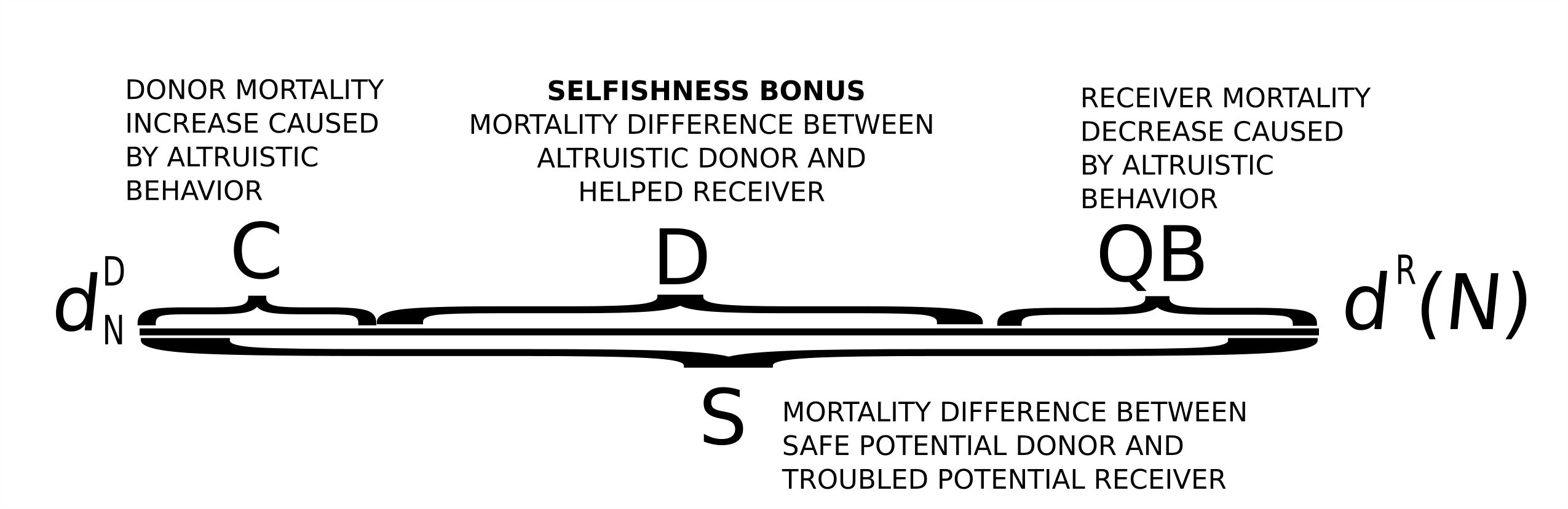
Figure 1:

Since $d_{N}^{D}=d_{C}^{D}-C$ parameter $S$ can be presented as $S=QB+D+C$ (see Fig. 1 for the meaning of these parameters). Then $d_{N}^{D}=d^{R}(N)-QB-D-C$ and thus $D$ can be interpreted as the efficiency of the sacrifice of the cooperating Donor in increasing the survival of the Receiver to the level of the safe individual. Therefore $D$ in addition to the cost $C$, saved by Noncooperator, can be termed the ”selfishness bonus”, since it will be consumed by noncooperative donors and cannot be transferred to the helped Receiver. Then equation (45) can be presented as

$$\left[\left(1-q_{C}^{D}\right)r-\left(1-q_{N}^{D}\right)\left(1-r\right)\right]QB+\left(q_{C}^{D}-q_{N}^{D}\right)\left[QB+D+C\right]>q_{C}^{D}C,$$

together with (43) leading to the general rule for cooperation expressed in terms of $B$,$C$ and $D$:

$$\left[\left(1-q_{N}^{D}\right)r-\left(1-q_{C}^{D}\right)(1-r)\right]QB+\left(q_{C}^{D}-q_{N}^{D}\right)D>q_{N}^{D}C.$$ (46)

and

$$\left(q_{C}^{D}-q_{N}^{D}\right)D<0\text{ when }[(1-r)-r]QB<C$$

$$\left(q_{C}^{D}-q_{N}^{D}\right)D>0\text{ when }[(1-r)-r]QB>C.$$

It seems to be little bit counterintuitive, but if we expand it to show differences between contributions for both strategies we obtain

$$q_{C}^{D}D-\left(1-q_{C}^{D}\right)(1-r)QB>q_{N}^{D}(D+C)-\left(1-q_{N}^{D}\right)rQB,$$

where $q_{C}^{D}D$ and $q_{N}^{D}(D+C)$ are Donor average mortalities weighted by fractions of Donors for both strategies and $\left(1-q_{C}^{D}\right)(1-r)QB$ is the Cooperators loss caused by wrong recognition of Cooperative Receiver, while $\left(1-q_{N}^{D}\right)rQB$ is Noncooperators loss caused by correct recognition by Cooperative Donor.

7.1 Case of $D<0$

Negative $D$ may occur when $C+B>S$, which means that changes in mortalities caused by altruistic action overlap and in effect they invert the inequality between mortalities of Donor and Receiver (this is depicted on Fig. 2).

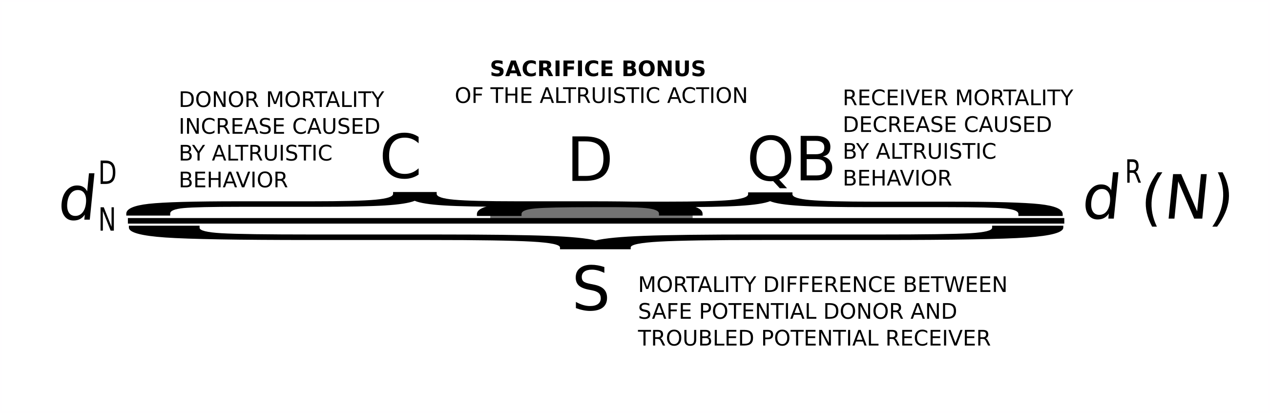
Figure 2:

Then $D$ can be termed sacrifice bonus since it acts negatively and the general rule for cooperation has the form

$$\left[\left(1-q_{N}^{D}\right)r-\left(1-q_{C}^{D}\right)(1-r)\right]QB+\left(q_{C}^{D}-q_{N}^{D}\right)D>q_{N}^{D}C.$$ (47)

and (48)

$$\left(q_{C}^{D}-q_{N}^{D}\right)D>0\text{ when }[(1-r)-r]QB<C$$ (49)

$$\left(q_{C}^{D}-q_{N}^{D}\right)D<0\text{ when }[(1-r)-r]QB>C,$$ (50)

therefore (49) shows that the impact of $D$ is positive when $\left[r-\left(1-r\right)\right]QB>C$ (19) is satisfied, however it will be positive even if $[r-(1-r)]QB>-C$.

7.2 Case of $D=0$

Note that for $D=0$ it will have form

$$\frac{\left(1-q_{N}^{D}\right)r-\left(1-q_{C}^{D}\right)(1-r)}{q_{N}^{D}}QB>C$$ (51)

Impact of the benefit is positive when $\left(1-q_{C}^{D}\right)r-\left(1-q_{N}^{D}\right)\left(1-r\right)>0$ leading to

$$r>\frac{\left(1-q_{N}^{D}\right)}{\left(1-q_{C}^{D}\right)+\left(1-q_{N}^{D}\right)}=\frac{q_{N}^{R}}{q_{C}^{R}+q_{N}^{R}}$$

Depending on the parameter values, condition (51) may be weaker or stronger than rule (19). It will be weaker or equivalent when

$$\dfrac{\left(1-q_{N}^{D}\right)r-\left(1-q_{C}^{D}\right)(1-r)}{q_{N}^{D}}\leq r-(1-r),$$

leading to the condition

$$r\leq r^{\ast}=\dfrac{1-q_{N}^{D}-q_{C}^{D}}{2-3q_{N}^{D}-q_{C}^{D}},$$ (52)

where $r^{\ast}$ is the manifold where both conditions (51) and (19) are equivalent. Numerator is negative if $q_{C}^{D}>1-q_{N}^{D}$ and on the line $q_{C}^{D}=1-q_{N}^{D}$ we have $r^{\ast}=0$. Denominator is negative if $q_{C}^{D}>2-3q_{N}^{D}$ and $q_{C}^{D}=2-3q_{N}^{D}$ is the singular surface. Manifold where $r^{\ast}=1$ is the line $q_{N}^{D}=1/2$ It intersects with the singular surface at $q_{C}^{D}=1/2$. Summarizing, the negative value of $r^{\ast}$ is possible when only numerator or only denominator is negative

$$1-q_{N}^{D} < q_{C}^{D}<3q_{N}^{D}-1\text{ \ \ \ for \ \ }q_{N}^{D}<0.5$$

and

$$3q_{N}^{D}-1 < q_{C}^{D}<1-q_{N}^{D}\text{ \ \ \ \ \ for\ \ \ }q_{N}^{D}>0.5.$$

In addition (51) will be always weaker than (19) ($r^{\ast}>1$) when

$$q_{C}^{D}>3q_{N}^{D}-1\text{ \ \ \ for \ \ }q_{N}^{D}<0.5\text{ \ and\ \ }q_{C}^{D}<3q_{N}^{D}-1\text{ \ \ \ for \ \ \ }q_{N}^{D}>0.5,$$

in other case ($r^{\ast}<0$) the rule for cooperation will be always stronger than (19) (see Figure 3 and Figure 4 for plot of the surface $r^{\ast}$).

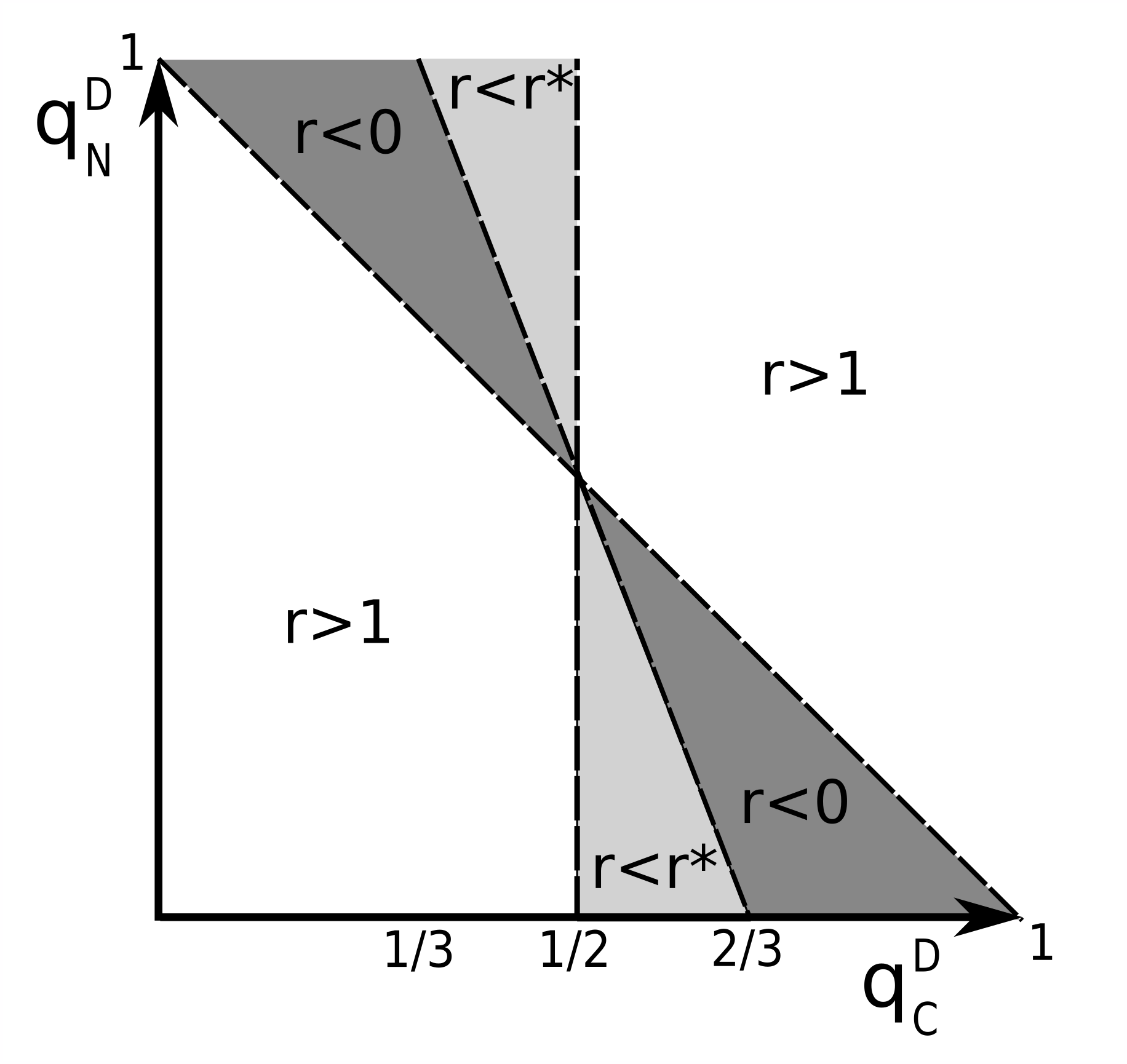
Figure 3: Diagram describing the role allocations for different strategies when new rule for cooperation is always stronger/weaker (is satisfied for greater/smaller $r$) or may be either smaller, greater or equivalent.

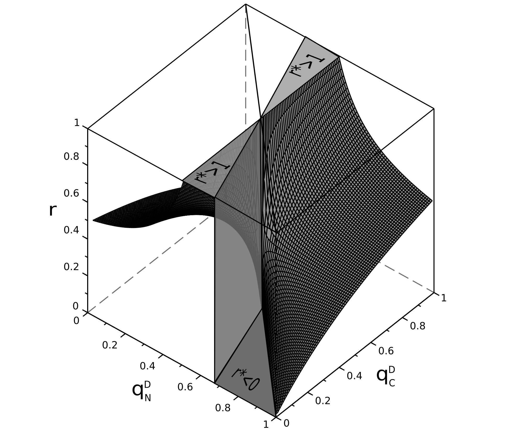
Figure 4: Plot of the surface $r^{\ast}$ where new rule for cooperation is equivalent to the classical rule (works for the same parameter $r$.

Therefore conditions for cooperation are highly affected by the dynamics of the distribution of states. In addition we have trade-off between cost and benefits resulting from the cooperative action and the changes of basal mortalities ((56) and (57) in Appendix 1) caused by impact of the focal interaction on the equilibria of the switching dynamics (represented by term $\left(q_{N}^{D}-q_{C}^{D}\right)\left(d_{N}^{D}-d^{R}(N)\right)$ in equation (44)) leading to the third parameter $S$ (and in effect $D$). Summarizing, we obtain formula expressed in terms of Benefit, Cost and the Selfishness/Sacrifice Bonus. The last parameter can describe important biological factors. Selfishness/Sacrifice Bonus can occur in many types of problems for example in engaging in the fight to save other individual. Passive individual will be safer than all individuals involved in the fight. For example, in the mentioned in the beginning problem of predator warning signal it may be zero because selfish individual that spotted predator will hide, thus it will behave as individuals warned by Cooperator. However, we can imagine the cases, where hidden Noncooperator may have greater survival when all other individuals are exposed and attract the attention of the predator, than in case when everybody are hidden and have the same risk of being catched. The above formula takes into account the asymmetry in the distribution of roles. The values of $q_{C}^{R}$ and $q_{N}^{R}$ can be calculated from the equilibria of the equations (39,40). Note that rule for cooperation (46) in the cases when $Q<1$ will have more complicated form and it will depend on the cooperative gene frequency $g_{C}$.

7.3 The kin selection case

Recall from the previous sections that in the case of kin selection $r$ is replaced by $p_{C}$ and $(1-r)$ by $p_{N}$ (23), and since cooperators will pay the cost only for their kins. Thus, in the switching dynamics (39,40) the terms $C+QrB$ and $Q\left(1-r\right)B$ should be replaced by $C+p_{C}QB$ for Cooperators and $p_{N}QB$ for Noncooperators. The equivalent of (43) will be $C<\left[p_{N}-p_{C}\right]QB$  ($C>r_{k}QB$). Therefore, (46) will be

$$\left[p_{C}(1-q_{N}^{D})-p_{N}(1-q_{C}^{D})\right]QB+\left(q_{C}^{D}-q_{N}^{D}\right)D>q_{C}^{D}C,$$ (53)

leading to

$$\left[r_{k}(1-q_{N}^{D})+(1-r_{k})g_{C}\left(q_{C}^{D}-q_{N}^{D}\right)\right]QB+\left(q_{C}^{D}-q_{N}^{D}\right)D>q_{C}^{D}C.$$

In the absence of the selfishness bonus ($D=0$) the above formula simplifies to

$$\frac{r_{k}(1-q_{N}^{D})+(1-r_{k})\left(q_{C}^{D}-q_{N}^{D}\right)g_{C}}{q_{C}^{D}}QB>C.$$

It can be presented in the form expressing the impact of parameter $r_{k}$

$$\frac{r_{k}\left[1-\left(q_{N}^{D}(1-g_{C})+q_{C}^{D}g_{C}\right)\right]+\left(q_{C}^{D}-q_{N}^{D}\right)g_{C}}{q_{C}^{D}}QB>C.$$

Therefore, even in the case of $Q=1$ the success depends on the frequency of cooperators in the population described by $g_{C}$. Only in the case when $q_{N}^{D}=q_{C}^{D}$ the above formula reduces to the Hamilton’s rule (29).

8 Discussion

Summarizing, in this paper we expressed the basic classic results on Inclusive Fitness and Kin Selection in the simplified form related to the Event Based Approach (Argasinski and Broom 2013,2017,2018). In effect, the classical framework was simplified and expressed in the measurable parameters e.g. mortality (or survival) related to the focal type of interaction, when cooperative trait is expressed. In addition, another important parameter was incorporated into the framework. This parameter describes the distribution of roles Donor/Receiver among members of the population. This leads to the general rule for positive growth of the frequency of the cooperative strategy showing that among Receivers of the altruism should be more Cooperators than Noncooperators. This implies the need for identification or discrimination strategies to sort out the noncooperative individuals. In addition, if the frequency of Cooperators is low, the Cooperators should gather together and support themselves. This mechanism can be relaxed with the spread of the cooperative gene, since with increase of the fraction of Cooperators increases the probability of meeting the Cooperator at random. Increase of the sizes of cooperative groups or the level of cooperation in the whole population leads to the problem of elimination of free riding Noncooperators. The incorporation of these mechanisms into framework developed in this paper is the question for the future research. One of the basic strategies is the limitation of the altruism to close kins only, which leads to the classical Hamilton’s rule. The transition from cooperative subgroups (groups of closely related kins at the beginning) to fully cooperative population caused by increase of the frequency of Cooperators is another interesting question. It is related to the transition between different types of altruism, from restrictive kin altruism to broader forms of reciprocal altruism, leading to the cooperative instinct towards all members of the population. This aspect should be also incorporated into new framework.

New formulation allowed for generalization described in the second part of the paper. The distinction between two separate outcomes of the interaction, which are survival and change of the role, leads to the problem of the mechanisms underlying the dynamics of role changes. This formulation is more mechanistic than classical approaches based on abstract fitness (Geritz and Kisdi 2012) and allows for the deeper insight into the modelled problem. It shows that the classical formulation works well for the cases when roles are independently drawn at every focal interaction event. Good example of the problem of this type is the classical Haldane’s dilemma describing the help for the drowning individual. However, in some problems this may not be the case. For example help for the sick individual may support him with necessary supplies but may not cure him. If this individual suffers from the infectious disease then the altruistic action may lead to infection of the Cooperative Donor and in effect the fraction of the strategy carriers being in trouble can increase. Important result shown by new framework is that in those cases different strategies may have different distributions of roles. These complicated cases can be described by models extended by equations describing the role switching dynamics. Resulting equilibria of the role distributions (if they exist) should be considered in general rule for cooperation being the generalization of the classical approach leading to the Hamilton’s rule. In effect we obtain the general condition which is affected by differences in role distributions, which may be termed State Distribution Asymmetry. Resulting condition, in addition to the classical components describing Cost and Benefit, contains third component. This component may have different interpretations depending on its value. If Cooperative Donors mortality is smaller than the mortality of the helped Receivers then it describes the deficiency of benefit (in addition to the compensation of cost described by classical condition) that will be consumed by Noncooperative Donors doing nothing. That’s why it can be termed Selfishness Bonus and it should be added to the actual cost in the general rule for cooperation.

In the second case when Cooperative Donors mortality is greater than the mortality of the helped Receivers this component describes the ”amount” of Donor’s mortality ”transferred” into Receivers survival, therefore it can be termed Sacrifice Bonus. This component is consumed by Receivers, thus it can be subtracted from the actual cost in the general rule for cooperation.

Important aspect revealed by our model is that for derivation of the general rule for cooperation, being equivalent to the classical conditions, existence of the equilibria of the role dynamics is necessary. We can imagine cases with, for example, cyclic role switching dynamics. Then the static conditions for the selection toward altruism will be more complex and will probably contain integrals over trajectories of the cycles describing the average role distributions in time.

The distribution of roles resulting from the selection mechanisms may be important tool for explanation of many biological phenomena. for example it can play important role in evolution of the social structure and the division of labour among social insects. This is another potential direction of future research.

9 What is the difference between $C<rB$ and $C<r_{k}B$?

In addition to popular fallacies (Park 2007, West et al. 2011) associated with Hamilton’s rule, there is one popular mistake related to the relationships between inclusive fitness and kin selection concepts. The question is: Should the relatedness be defined as the probability that the Receiver is the carrier of the cooperative gene or it should be also inherited from the common ancestor? This problem was critically discussed by Gintis (2013) and can be found for example in Bourke (2011). Also Encyclopedia Britannica states that:

”Relatedness is the probability that a gene in the potential altruist is shared by the potential recipient of the altruistic behaviour.”

without explicit reference to genealogy. The source of the problem is following: For simplified case of pairwise interactions between single Donor and Receiver when there are enough Donors for every Receiver (then $Q=1$ and $q^{D}=0.5$), the condition for positive growth $C<rB$ (27) reduces to $C<\left[r_{k}+(1-r_{k})g_{C}\right]B=p_{C}B$ for kin selection case. On the other hand the general condition for cooperation $C<\left[r-(1-r)\right]B$ (28) in kin selection case reduces to $C<r_{k}B$. Note that $p_{C}$ describes probability that the Benefit consuming Donor is actually the carrier of the cooperative gene, thus it can be interpreted as parameter $r$ in the general inclusive fitness sense. However, since in the inclusive fitness case Cooperators interact with kins only we have that $p_{N}\neq 1-r$. Then the relationships between $r$ and $r_{k}$ can be summarized as

$$\boldsymbol{C}\boldsymbol{<rB} \simeq p_{C}B\text{ \ \ }\Longrightarrow\text{\ \ \ \ }C<r_{k}B+(1-r_{k})g_{C}B.$$

$$C < \left[r-(1-r)\right]B\simeq\left[p_{C}-p_{N}\right]B\text{ \ \ }\Longrightarrow\text{\ \ \ \ }\boldsymbol{C<r}_{k}\boldsymbol{B}.$$

Thus, what is the difference between $C<rB$ and $C<r_{k}B$? Condition $C<rB$ where $r$ is the probability that the Receiver is the carrier of the cooperative gene (identity by state in terms of population genetics) is the condition for positive impact of the act of altruism on the growth rate of Cooperators. thus it is not sufficient for the spread of altruism. On the other hand, condition $C<r_{k}B$ where $r_{k}$ is the probability that Receiver inherited cooperative gene from the common ancestor (identity by descent) is the condition for greater growth for Cooperators over Noncooperators. This is correct condition for altruism, however limited to kins only. However, all above reasonings are based on the assumption that the distribution of roles $q^{D}$ is constant and independent of the outcomes of the analyzed interaction.

References:Alger I, Weibull JW (2012)A generalization of Hamilton’s rule—Love others how much? J Theor Biol 29942-54
Allen B (2015). Inclusive fitness theory becomes an end in itself. BioScience 65(11) 1103-1104
Allen B, Nowak MA (2016) There is no inclusive fitness at the level of the individual. Current Opinion in Behavioral Sciences 12 122-128
Argasinski K (2006) Dynamic multipopulation and density dependent evolutionary games related to replicator dynamics. A metasimplex concept. Math Biosci 202 88-114
Argasinski K (2012) The dynamics of sex ratio evolution Dynamics of global population parameters. J Theor Biol 309 134-146
Argasinski K (2013) The Dynamics of Sex Ratio Evolution: From the Gene Perspective to Multilevel Selection. PloS ONE 8(4) e60405
Argasinski K (2018) The dynamics of sex ratio evolution: the impact of males as passive gene carriers on multilevel selection. Dyn Gam App 8(4) 671-695
Argasinski K, Broom M (2013a) Ecological theatre and the evolutionary game: how environmental and demographic factors determine payoffs in evolutionary games. J Math Biol 1;67(4):935-62
Argasinski, K Broom M (2018a) Interaction rates, vital rates, background fitness and replicator dynamics: how to embed evolutionary game structure into realistic population dynamics. Theo Bio 137(1) 33-50
Argasinski K Broom M (2018b) Evolutionary stability under limited population growth: Eco-evolutionary feedbacks and replicator dynamics. Ecol Complex 34 198-212
Birch J (2017) The inclusive fitness controversy: finding a way forward. Royal Society open science 4(7) 170335
Cressman R (1992) The Stability Concept of Evolutionary Game Theory Springer
Doebeli M, Ispolatov Y, Simon B (2017) Point of view: Towards a mechanistic foundation of evolutionary theory. Elife 6 e23804
Doebeli M, Hauert C (2006) Limits of Hamilton’s rule. J Evol Biol 19(5) 1386-1388
https://www.britannica.com/science/animal-behavior/Function#ref1043131
Fletcher JA, Doebeli M (2008) A simple and general explanation for the evolution of altruism. Proc of the R Soc B: Biological Sciences 276(1654) 13-19
Fletcher JA, Zwick M, Doebel M, Wilson DS (2006) What’s wrong with inclusive fitness? TREE 21(11) 597-598
Gardner A, West SA, Wild G (2011) The genetical theory of kin selection. J Evol Biol 24(5) 1020-1043
Geritz SA , Kisdi É (2012) Mathematical ecology: why mechanistic models? J Math Biol, 65(6), 1411-1415
Gintis H (2014) Inclusive fitness and the sociobiology of the genome. Biol Philos 29(4) 477-515
Grafen A (2006) Optimization of inclusive fitness. J theor Biol Feb 7;238(3):541-63
Hofbauer J, Sigmund K (1988) The Theory of Evolution and Dynamical Systems. Cambridge University Press
Hofbauer J, Sigmund K (1998) Evolutionary Games and Population Dynamics. Cambridge University Press
Houston AI, McNamara J (1999) JM Models of adaptive behaviour: an approach based on state. Cambridge University Press;
Houston AI, McNamara J (2005) John Maynard Smith and the importance of consistency in evolutionary game theory. Biol Phil 20(5) 933-950
Hauert C, Holmes M, Doebeli M (2006) Evolutionary games and population dynamics: maintenance of cooperation in public goods games. Proc R Soc B: Biological Sciences 273(1600) pp.2565–2570
Hauert C, Wakano JY, Doebeli M, (2008) Ecological public goods games: cooperation and bifurcation. Theor Pop Biol 73(2) pp.257–263
Marshall JA (2015) Social evolution and inclusive fitness theory: an introduction. Princeton University Press
Marshall JA (2016) What is inclusive fitness theory, and what is it for? Current Opinion in behavioral Sciences 12 103-108
Maynard Smith J (1982) Evolution and the Theory of Games. Cambridge University Press Cambbridge, United Kingdom
McElreath R, Boyd R (2008) Mathematical models of social evolution: A guide for the perplexed. University of Chicago Press
Kramer J, Meunier J (2016) Kin and multilevel selection in social evolution: a never-ending controversy? F1000Research, 5
McNamara JM (2013) Towards a richer evolutionary game theory. J Roy Soc Interface 10(88) 20130544
Nowak MA (2006) Five rules for the evolution of cooperation. Science 314(5805) 1560-1563
Nowak MA, Tarnita, CE, Wilson EO (2010) The evolution of eusociality. Nature, 466(7310) 1057
Nowak M A , McAvoy A , Allen B, Wilson EO (2017) The general form of Hamilton’s rule makes no predictions and cannot be tested empirically. PNAS 114(22) 5665-5670
Okasha S, Martens J (2016) The causal meaning of Hamilton’s rule. R Soc Open Science 3(3) 160037
Park JH (2007) Persistent misunderstandings of inclusive fitness and kin selection: Their ubiquitous appearance in social psychology textbooks. Evol Psychol 5(4) 147470490700500414
Rousset F, Lion S (2011) Much ado about nothing: Nowak et al.’s charge against inclusive fitness theory. J Evol Biol 24(6) 1386-1392
Roff DA (2008) Defining fitness in evolutionary models. J Genet 87 339–348
Metz JAJ (2008) Fitness. In: Jørgensen SE, Fath BD (Eds.) Evolutionary Ecology. In: Encyclopedia of Ecology vol. 2 Elsevier pp. 1599–1612
Van Veelen M (2009) Group selection, kin selection, altruism and cooperation: when inclusive fitness is right and when it can be wrong. J Theor Biol Aug 7;259(3):589-600
Van Veelen M, Allen B, Hoffman M, Simon B, Veller C (2017) Hamilton’s rule. J Theor Biol 414 176-230
Wenseleers T (2006) Modelling social evolution: the relative merits and limitations of a Hamilton’s rule-based approach. J Evol Biol 19(5) 1419-1422
West SA, Griffin AS, Gardner A (2007) Social semantics: altruism, cooperation, mutualism, strong reciprocity and group selection. J Evol Biol 20(2) 415-432
West SA, El Mouden C, Gardner A (2011) Sixteen common misconceptions about the evolution of cooperation in humans. Evol Hum Beh 32(4), 231-262

Appendix 1

Let us derive the bracketed term $\left(\bar{d}_{N}(g,q)-\bar{d}_{C}(g,q)\right)$ from (42) where

$$\bar{d}_{C}(g,q)=q_{C}^{D}\left(d_{N}^{D}+C\right)+\left(1-q_{C}^{D}\right)\left(d^{R}(N)-QrB\right)$$

and

$$\bar{d}_{N}(g,q)=q_{N}^{D}d_{N}^{D}+\left(1-q_{N}^{D}\right)\left(d^{R}(N)-Q\left(1-r\right)B\right),$$

above payoffs can be presented as

$$\bar{d}_{C}(g,q)=\tilde{d}_{C}(q_{C})-\left(1-q_{C}^{D}\right)QrB+q_{C}^{D}C$$ (54)

and

$$\bar{d}_{N}(g,q)=\tilde{d}_{N}(q_{N})-\left(1-q_{N}^{D}\right)Q\left(1-r\right)B,$$ (55)

where

$$\tilde{d}_{C}(q_{C}) = q_{C}^{D}d_{N}^{D}+\left(1-q_{C}^{D}\right)d^{R}(N)$$ (56)

$$\tilde{d}_{N}(q_{N}) = q_{N}^{D}d_{N}^{D}+\left(1-q_{N}^{D}\right)d^{R}(N)$$ (57)

describe the different basal average mortalities (in addition to the impact of strategic parameters $C$ and $B$) caused by distributions of states for both strategies and

$$\tilde{d}_{N}(q_{N})-\tilde{d}_{C}(q_{C}) = \left(q_{N}^{D}-q_{C}^{D}\right)d_{N}^{D}+\left[\left(1-q_{N}^{D}\right)-\left(1-q_{C}^{D}\right)\right]d^{R}(N)$$ (58)

$$= \left(q_{C}^{D}-q_{N}^{D}\right)\left(d^{R}(N)-d_{N}^{D}\right),$$

in effect

$$\bar{d}_{N}(g,q)-\bar{d}_{C}(g,q)=$$

$$\tilde{d}_{N}(q_{N})-\tilde{d}_{C}(q_{C})-\left(1-q_{N}^{D}\right)Q\left(1-r\right)B+\left(1-q_{C}^{D}\right)QrB-q_{C}^{D}C=$$

$$\left(q_{N}^{D}-q_{C}^{D}\right)\left(d_{N}^{D}-d^{R}(N)\right)+\left[\left(1-q_{C}^{D}\right)r-\left(1-q_{N}^{D}\right)\left(1-r\right)\right]QB-q_{C}^{D}C$$ (59)

leading to the equation on selection of the strategies (42)

$$\dot{g}_{C} = {}g_{C}\left(1-g_{C}\right)\left[\left(q_{N}^{D}-q_{C}^{D}\right)\left(d_{N}^{D}-d^{R}(N)\right)\right.$$ (60)

$$\left.+\left[\left(1-q_{C}^{D}\right)r-\left(1-q_{N}^{D}\right)\left(1-r\right)\right]QB-q_{C}^{D}C\right]$$