State dependent diffusion in a bistable potential: conditional probabilities and escape rates

Abstract

We consider a simple model of a bistable system under the influence of multiplicative noise. We provide a path integral representation of the overdamped Langevin dynamics and compute conditional probabilities and escape rates in the weak noise approximation. The saddle-point solution of the functional integral is given by a diluted gas of instantons and anti-instantons, similarly to the additive noise problem. However, in this case, the integration over fluctuations is more involved. We introduce a local time reparametrization that allows its computation in the form of usual Gaussian integrals. We found corrections to the Kramers’ escape rate produced by the diffusion function which governs the state dependent diffusion for arbitrary values of the stochastic prescription parameter. Theoretical results are confirmed through numerical simulations.

I Introduction

The physics of thermal or noise activation over a barrier has a long history. Nowadays, it is an important research topic due to the wide range of applications in several areas of science, such as physics, chemistry and biology as well Fleming and Hänggi (1993). The simplest model to study this problem is a classical particle in a bistable potential, $U(x)$, whose dynamics is driven by an overdamped Langevin equation with additive white noise. In this context, an important physical quantity is the rate at which the particle escape out of a minimum of the potential. The seminal work of Kramers Kramers (1940) stated the very simple formula

$$r_{\rm add}=\frac{\sqrt{\omega_{\rm min}|\omega_{\rm max}|}}{2\pi}e^{-\frac{\Delta U}{\sigma^{2}}}$$ (1)

where $r_{\rm add}$ is the escape rate, $\Delta U=U(x_{\rm max})-U(x_{\rm min})$ is the height of the potential barrier, $\sigma^{2}$ is the noise intensity and $\omega_{\rm min}=U^{\prime\prime}(x_{\rm min})$ and $\omega_{\rm max}=U^{\prime\prime}(x_{\rm max})$ are the local curvatures of the potential at its minimum ($x_{\rm min}$) and its maximum ($x_{\rm max}$), respectively (primes mean derivative with respect to $x$). We use the notation $r_{\rm add}$ to emphasize that this expression for the escape rate was computed assuming an additive noise stochastic differential equation. Equation (1) is valid in the weak noise or high barrier approximation $\sigma^{2}\ll\Delta U$. Since this well-established result was defined, a lot of work has been done in order to compute more accurate expressions suitable to be applied to more realistic situations. The generalization of Eq. (1) to multidimensional systems was (and still is) a big challenge Hänggi et al. (1990). Moreover, generalizations to different types of noise probability distributions have been also considered Bray and McKane (1989); McKane et al. (1990); Bray et al. (1990); Luckock and McKane (1990); Jung et al. (2005); Goulding et al. (2007).

On the other hand, there is an increasing interest for multiplicative noise stochastic systems. Some examples of multiplicative noise dynamics are given by the diffusion of particles near a wall Lançon et al. (2001, 2002); Lau and Lubensky (2007); Volpe et al. (2010); Brettschneider et al. (2011), micromagnetic dynamics García-Palacios and Lázaro (1998); Aron et al. (2014); Arenas et al. (2018) and non-equilibrium transitions into absorbing states Hinrichsen (2000). There are two particular stochastic phenomena in which multiplicative noise plays an important role: noise-induced phase transitions Van den Broeck et al. (1994); Castro et al. (1995); Carrillo et al. (2003); Jafarpour et al. (2015); Barci et al. (2016) and stochastic resonance Benzi et al. (1981, 1983); Wio, H. S. and Deza, R. R. (2007); Wio et al. (2002). In the last case, the escape rate is at the stem of the physical description of the observed phenomenology.

One of the main questions that we address in this paper is how the Kramers’ escape rate of Eq. (1) is modified when the dynamics is driven by a general multiplicative noise, modeled by a diffusion function $g(x)$. This topic have been rarely treated in the past and there is some controversy in the literature Jin et al. (2005); Guo and Cheng (2011); Li-Juan and Wei (2006); Zheng et al. (2011); Rosas et al. (2016). In particular, we study the dependence of the escape rate on the stochastic prescription, necessary to correctly define the multiplicative noise Langevin equation. This point is particularly relevant in order to compare analytic results with numerical simulations. Our main result is

$$r_{\rm mult}=g^{2}(x_{\rm max})\frac{\sqrt{\tilde{\omega}_{\rm min}|\tilde{\omega}_{\rm max}|}}{2\pi}\;e^{-\frac{\Delta U_{\rm eq}}{\sigma^{2}}}\;.$$ (2)

We used the notation $r_{\rm mult}$ to denote the escape rate in the multiplicative noise case. In general, we observe that the Arrhenius form of the Kramers’ result still remains. Another similarity with Eq. (1) is that the escape rate does not depend on details, either of the potential or of the diffusion function. Instead, it only depends on the local properties of these functions at the maximum and minima of the potential. On the other hand, there are significant differences between both results. Firstly, the original potential $U(x)$ has been replaced by the equilibrium potential $U_{\rm eq}(x)$, obtained from the solution of the asymptotic stationary Fokker-Planck equation (Eq. (7)). This potential depends on the noise and, more important, on the prescription used to interpret the stochastic differential equation. The barrier height is, in this case, $\Delta U_{\rm eq}=U_{\rm eq}(x_{\rm max})-U_{\rm eq}(x_{\rm min})$. It is worth to note that $x_{\rm max}$ and $x_{\rm min}$ are the position of the maximum and minumum of the equilibrium potential $U_{\rm eq}$ and not of the original “classical” potential $U(x)$. Local curvatures $\tilde{\omega}_{\rm min}=U^{\prime\prime}_{\rm eq}(x_{\rm min})$ and $\tilde{\omega}_{\rm max}=U^{\prime\prime}_{\rm eq}(x_{\rm max})$ are also computed by using the equilibrium potential. Finally, there is an overall factor given by the diffusion function computed at the maximum of the equilibrium potential, $g^{2}(x_{\rm max})$, coming from a careful treatment of fluctuations. We describe the model and the technique used to compute Eq. (2), discussing the result in more detail, throughout the paper.

Multiplicative stochastic processes can be studied with different theoretical approaches. For numerical simulations Sivak et al. (2013), the Langevin approach seems to be more adequate. The Fokker-Planck equation is perhaps more appropriate to develop analytic calculations, specially in the long time stationary limit. In this context, techniques such as mean fields, perturbation theory and even renormalization group are also available Goldenfeld (1992). On the other hand, the path integral formulation of stochastic processes is the more natural technique to compute correlation and response functions Wio (2013). Important progress has been recently reached in the path integral representation of multiplicative noise processes Aron et al. (2010); Arenas and Barci (2010, 2012a, 2012b); Moreno et al. (2015); Aron et al. (2016), despite the fact that this topic has been studied for a long time Janssen (1992).

The escape rate is just one ingredient of a more general problem that is the computation of conditional probabilities. Equilibrium properties, such as detailed balance, can be cast in terms of the conditional probability and its time reversal. Time reversal transformations, detailed-balance relations, as well as microscopic reversibility in multiplicative processes were studied in detail in Ref. Arenas and Barci (2012b). More recently, we have presented a useful path integral technique to compute weak noise expansions Moreno et al. (2019). The integration over fluctuations in the multiplicative case is not trivial. The reason is that the diffusion function produces an integration measure that resembles a curved time axis Zinn-Justin (2002). We have provided a local time reparametrization in order to integrate fluctuations Moreno et al. (2019). In this paper, we compute the conditional probability of finding a particle in a well at large times $t/2$, provided it was in the same or the other well at $-t/2$. In the weak noise approximation, saddle points provide a set of diluted instanton and anti-instanton solutions. The diluted instanton gas approximation was first introduced in the context of quantum mechanics to compute the tunneling probability across a potential barrier Coleman (1979). In the context of an additive stochastic process, it was developed with great detail in Refs. Caroli et al. (1979, 1981). From a technical point o view, we generalize the calculation of Ref. Caroli et al. (1981) to the multiplicative noise case, using the time reparametrization techniques introduced in Ref. Moreno et al. (2019). We also perform extensive Langevin simulations to test our results and approximations, finding an excellent agreement.

The paper is organized as follows. In the next section, we present the equilibrium properties of a particle in a double-well potential under state dependent diffusion. In section III, we briefly review the path integral representation of a conditional probability in a multiplicative process and we show, in section IV, how to integrate fluctuations. We develop the dilute instanton gas approximation in section V, where we compute conditional probabilities and the escape rate. In VI we present Langevin simulations of a particular model and compare the output with our analytic results. Finally, we discuss our results in section VII. We lead to the Appendix A some details of the calculation.

II Equilibrium properties of a particle in a double-well potential under state dependent diffusion

In this section, we describe the equilibrium properties of a model consisting of a single particle in a double-well potential coupled with a thermal bath with state dependent diffusion. We consider a conservative one dimensional system described by a potential energy $U(x)=U(-x)$ with a double minima structure. The thermal bath is characterized by the diffusion function $g(x)=g(-x)$. The reflection symmetry $x\to-x$ is not essential and most of our results do not depend on it. However, to keep the discussion as simple as possible, we focus in the symmetric model, leading the details of a more general asymmetric situation to a future presentation.

In order to reach thermodynamic equilibrium at long times, the drift force $f(x)$ should be related with the classical potential $U(x)$ through a generalized Einstein relation Arenas and Barci (2012a, b)

$$f(x)=-\frac{1}{2}g^{2}(x)\frac{dU(x)}{dx}\;.$$ (3)

In this way, the overdamped stochastic dynamics is driven by the Langevin equation

$$\frac{dx}{dt}=-\frac{1}{2}g^{2}(x)\frac{dU(x)}{dx}+g(x)\eta(t),$$ (4)

where $\eta(t)$ obeys a Gaussian white noise distribution with

$$\left\langle\eta(t)\right\rangle=0\;\;\mbox{,}\;\;\;\left\langle\eta(t)\eta(t^{\prime})\right\rangle=\sigma^{2}\delta(t-t^{\prime})\;,$$ (5)

in which $\sigma^{2}$ measures the noise intensity. This equation is understood in the generalized Stratonovich Hänggi (1978) prescription (also known as $\alpha-$prescription Janssen (1992)). The asymptotic long time equilibrium probability distribution is given by Arenas and Barci (2012b)

$$P_{\rm eq}(x)={\cal N}\;e^{-\frac{1}{\sigma^{2}}U_{\rm eq}(x)},$$ (6)

where ${\cal N}$ is a normalization constant and the equilibrium potential

$$U_{\rm eq}(x)=U(x)+(1-\alpha)\sigma^{2}\ln g^{2}(x)\;.$$ (7)

The parameter $0\leq\alpha\leq 1$ labels the particular stochastic prescription used to discretized the Langevin equation. For instance, $\alpha=0$ corresponds with Itô interpretation while $\alpha=1/2$ corresponds with the Stratonovich one. In this way, the equilibrium potential is not the bare classical potential, but it is corrected by the diffusion function $g(x)$. On the other hand, the case $\alpha=1$ corresponds with Hänggi-Klimontovich or kinetic interpretation Hänggi and Thomas (1982); Klimontovich (1994). This is the only prescription which leads to the Boltzmann distribution $U_{\rm eq}(x)=U(x)$. Furthermore, this prescription is also known as anti-Itô and can be considered as the time reversal conjugated to the Itô prescription Arenas and Barci (2012b); Moreno et al. (2015).

Although the techniques and results of this paper do not depend on details, either of $U(x)$ or of $g(x)$, it is convenient, just to visualize the equilibrium potential $U_{\rm eq}(x)$, to consider a very simple model. Let us take, for instance,

$$U(x)=-\frac{1}{2}x^{2}+\frac{1}{4}x^{4}\;,$$ (8)

with the diffusion function

$$g(x)=1+\lambda x^{2}.$$ (9)

where the parameter $\lambda$ measures in some sense the multiplicative character of the noise. The particular value of $\lambda=0$ corresponds with an additive noise. The potential $U(x)$ has two degenerated minima at $x_{\rm min}=\pm 1$ and a local maximum at $x_{\rm max}=0$. The contribution of the multiplicative noise for the equilibrium potential is quite interesting. In the weak noise limit, the global two-minima structure remains the same. However, the minima are displaced to

$$x_{\rm min} =\pm(1-4\sigma^{2}(1-\alpha))^{1/4}$$

$$\sim\pm 1\mp\sigma^{2}(1-\alpha)+O(\sigma^{4})\;.$$ (10)

For $\sigma^{2}\geq 1/4(1-\alpha)$, both minima melt in a single one, deeply changing the global structure of the potential. This dependence on the noise intensity resembles a second order phase transition, where the critical noise is given by

$$\sigma_{c}=\frac{1}{2}\frac{1}{\sqrt{1-\alpha}}\;.$$ (11)

Interestingly, the critical noise depends on the stochastic prescription. For $\alpha\to 1$, $\sigma_{c}\to\infty$, meaning that, in the anti-Itô prescription, the double-well structure is preserved for all values of the noise.

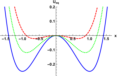
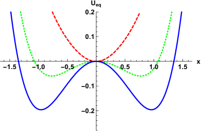
Figure 1: Equilibrium potential $U_{\rm eq}(x)$ given by Eq. (7). In (a) we fixed $\sigma=0.5$. The continuous line is plotted in the anti-Itô prescription $\alpha=1$, the dotted line is in the Stratonovich prescription $\alpha=1/2$ and the dashed line corresponds to the Itô interpretation $\alpha=0$. In (b), all the curves are computed in the Itô interpretation. The continuous curve is plotted with $\sigma=1/5$, the dotted line with $\sigma=2/5$ and the dashed line with $\sigma=2/3$. In both figures we have fixed $\lambda=1$.

In Figure 1, we depict the equilibrium potential $U_{\rm eq}(x)$ given by Eq. (7) for the simple model specified by Eqs. (8) and (9), for different values of the parameters $\sigma$ and $\alpha$. In Figure 1-(a), we show the equilibrium potential for $\sigma=0.5$ and different values of the stochastic prescription $\alpha=0,1/2,1$. We see that, for $\alpha=1$, $U_{\rm eq}=U$ and the minima are fixed at $x_{\rm min}=\pm 1$. However, in the Stratonovich and Itô prescriptions, the minima are displaced towards the origin. In Figure 1-(b), the three curves are computed in the Itô prescription with different values of the noise $\sigma=1/5,2/5,2/3$. In this case, the minima approach zero when the noise grows and, for the value $\sigma=2/3>\sigma_{c}=1/2$, the equilibrium potential has only one global minimum at $x_{\rm min}=0$.

III Conditional probabilities: path integral representation

We are interested in computing the conditional probability $P(x_{f},t_{f}|x_{i},t_{i})$ of finding the system in the state $x_{f}$ at time $t_{f}$, provided the system was in the state $x_{i}$ at a previous time $t_{i}$. It is useful to express this quantity using a path integral representation Moreno et al. (2019). It can be written as

$$P(x_{f},t_{f}|x_{i},t_{i})=e^{-\frac{\Delta U_{\rm eq}}{2\sigma^{2}}}K(x_{f},t_{f}|x_{i},t_{i})$$ (12)

where $\Delta U_{\rm eq}=U_{\rm eq}(x_{f})-U_{\rm eq}(x_{i})$ and the propagator $K(x_{f},t_{f}|x_{i},t_{i})$ is given by

$$K(x_{f},t_{f}|x_{i},t_{i})=\int[{\cal D}x]\;e^{-\frac{1}{\sigma^{2}}\int_{t_{i}}^{t_{f}}dt\;L(x,\dot{x})}\;.$$ (13)

Here, the functional integration measure is

$$[{\cal D}x]={\cal D}x\;{\det}^{-1}g=\lim\limits_{\begin{subarray}{c}{N\to\infty}\\ {\Delta t\to 0}\end{subarray}}\prod_{n=0}^{N}\frac{dx_{n}}{\sqrt{\Delta t\;g^{2}(\frac{x_{n}+x_{n+1}}{2})}}$$ (14)

where $x_{0}=x_{i}$ and $x_{N}=x_{f}$. The Lagrangian can be written in the form,

$$L=\frac{1}{2}\left(\frac{1}{g^{2}(x)}\right)\dot{x}^{2}+V(x)\;,$$ (15)

where

$$V(x)=\frac{g^{2}}{2}\left[\left(\frac{U^{\prime}_{\rm eq}}{2}\right)^{2}-\sigma^{2}\left(\frac{U^{\prime\prime}_{\rm eq}}{2}+\frac{g^{\prime}}{g}U^{\prime}_{\rm eq}\right)\right]+\frac{\sigma^{4}}{4}\left(gg^{\prime}\right)^{\prime}.$$ (16)

The primes mean derivative with respect to $x$. Equation (13), with the Lagrangian defined by Eq. (15), correctly describes the dynamics of the Langevin Eq. (4) for arbitrary values of the parameter $0\leq\alpha\leq 1$ Moreno et al. (2019). It is important to note that all the information about the stochastic prescription is codified in the structure of the equilibrium potential $U_{\rm eq}(x)$, contained in the definition of the potential $V(x)$, Eq. (16). In this particular representation, the path integral measure given by Eq. (14) is discretized symmetrically, allowing us to use normal calculus rules in the manipulation of the path integral (for more details on the subtleties of stochastic calculus in the path integral formulation, please see Ref. Arenas and Barci (2012b) and references therein).

An interesting observation is that Eq. (13) coincides with the propagator of a quantum particle with position-dependent mass $m(x)=1/g^{2}(x)$ moving in a potential $V(x)$, written in the imaginary time path integral formalism $t\to-it$. The noise $\sigma^{2}$ plays the role of $\hbar$ in the quantum theory. At a classical level, the Lagrangian, Eq. (15), represents a particle with variable mass moving in a potential $-V(x)$. The structure of the potential $-V(x)$ (Eq. (16)) is much more complex than $U(x)$ or even $U_{\rm eq}(x)$.

In Figure 2, we plotted the potential $-V(x)$ for the simple model displayed by Eq. (8).

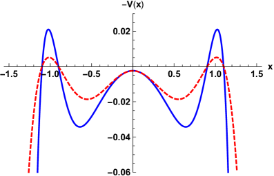
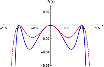
Figure 2: Potential $-V(x)$ given by Eq. (16). All the plots are in the Itô prescription, $\alpha=0$. The dashed lines are the potentials in the additive noise case $g(x)=1$ and the continuous lines correspond with multiplicative noise, for $g(x)=1+x^{2}$. In (a) we have fixed $\sigma=0.1$ while in (b), $\sigma=0.01$.

All the curves have been plotted in the Itô prescription $\alpha=0$. The dashed lines correspond to the additive noise case $g(x)=1$, while the continuous lines represent the potential in the multiplicative noise case, with $g(x)=1+x^{2}$. In Figure 2-(a) we fixed $\sigma=0.1$, while in Figure 2-(b), $\sigma=0.01$. The first observation is that $-V(x)$ has three maxima and two minima. The location of both non-zero maxima roughly coincides with the minima of the potential $U(x)$. The difference is of the order of $\sigma^{2}$. The main effect of the diffusion function is to increase the curvature at each maxima with a factor proportional to $g^{2}(x_{\rm max})>1$. An important feature that will be relevant to compute conditional probabilities is that the difference between the height of the peaks are of the order of $\sigma^{2}$. Thus, in a weak noise regime, the difference between the three maxima tends to disappear. In the extreme limit of $\sigma\to 0$, the potential $-V(x)$ has three degenerate maxima. This fact is clearly shown in Figure 2-(b). It is timely to note that the structure of $-V(x)$ is quite different from a similar calculus of the tunneling probability amplitude of a quantum particle Coleman (1979). In that case, the relevant potential is $-U(x)$, which has only two maxima. The appearance of a quasi-degenerate maximum at $x=0$ is proper of a classical stochastic process, even additive as well as multiplicative.

IV Fluctuations and time reparametrization

The usual weak noise expansion consists in evaluating the path integral of Eq. (13) in the saddle-point approximation plus Gaussian fluctuations. Generally, multiplicative noise induces an integration measure that depends on the diffusion function $g(x)$. In Ref. Moreno et al. (2019), we have shown how to overcome this problem by means of a time reparametrization. In this section, we briefly review this technique since we will use it to compute conditional probabilities.

The classical equation of motion is

$$\frac{d^{2}x}{dt^{2}}=g^{2}V^{\prime}+\frac{g^{\prime}}{g}\dot{x}^{2}\;.$$ (17)

Despite the fact that this is a complicated nonlinear equation, using time translation symmetry, a first integral can be built up. We have

$$\dot{x}_{cl}^{2}=2g^{2}_{cl}\left(V_{cl}+H\right)\,.$$ (18)

Here, $x_{cl}(t)$ is a solution of Eq. (17). The notation $x_{cl}$ stands for classical solution, resembling in some sense a semiclassical calculation in quantum mechanics. $H$ is an arbitrary constant, $g_{cl}=g(x_{cl}(t))$ and $V_{cl}=V(x_{cl}(t))$. Then, the solution of Eq. (17) can be expressed by a quadrature,

$$t-t_{0}=\int_{0}^{x_{cl}}\frac{ds}{\sqrt{2V_{\rm eff}(s)}}\;,$$ (19)

where we have defined an effective potential,

$$V_{\rm eff}(x)=g^{2}(x)\left[V(x)+H\right].$$ (20)

These expressions have two arbitrary constants, $t_{0}$ and $H$, that should be determined by means of the boundary conditions $x_{cl}(t_{i})=x_{i}$ and $x_{cl}(t_{f})=x_{f}$. Thus, Eqs. (19) and (20) implicitly define $x_{cl}(t)$, used as a starting point of the weak noise approximation.

Let us assume, for the moment, that, given initial and final conditions, the classical solution $x_{cl}$ is unique. Then, we consider fluctuations around it

$$x(t)=x_{cl}(t)+\delta x(t)\ ,$$ (21)

with boundary conditions $\delta x(t_{i})=\delta x(t_{f})=0$. Replacing Eq. (21) into Eq. (13) and keeping up to second-order terms in the fluctuations, we find for the propagator

$$K(x_{f},t_{f}| x_{i},t_{i})=$$ (22)

$$~{}~{}e^{-\frac{1}{\sigma^{2}}S_{cl}}\int[{\cal D}\delta x]\;e^{-\frac{1}{2}\int dtdt^{\prime}\;\delta x(t)O(t,t^{\prime})\delta x(t^{\prime})}\;,$$

where the classical action $S_{cl}$ is

$$S_{cl}=\int_{t_{i}}^{t_{f}}dt\;L(x_{cl}(t),\dot{x}_{cl}(t))$$ (23)

and the fluctuation kernel,

$$O(t,t^{\prime}) =-\frac{d~{}}{dt}\!\left(\frac{1}{g^{2}_{cl}}\frac{d\delta(t-t^{\prime})}{dt}\right)\!+\!\left(\frac{1}{g^{2}_{cl}}V^{\prime}_{\rm eff}(x_{cl})\right)^{\prime}\!\!\delta(t-t^{\prime}).$$

(24)

In Eq. (22), the functional integration measure is

$$[{\cal D}\delta x]=\lim\limits_{\begin{subarray}{c}{N\to\infty}\\ {\Delta t\to 0}\end{subarray}}\prod_{n=0}^{N}\frac{d\delta x_{n}}{\sqrt{\Delta t\;g^{2}(\frac{x_{cl}(t_{n})+x_{cl}(t_{n+1})}{2})}}.$$ (25)

Due to the time dependence of $g_{cl}=g(x_{cl}(t))$, the fluctuation kernel $O(t,t^{\prime})$ is not trivial. On the other hand, the integration measure, Eq. (25), depends on the diffusion function $g(x(t))$. As a consequence, although the exponent in Eq. (22) is quadratic, the evaluation of the functional integral is cumbersome. In this case, to compute the fluctuation integral, we make a time reparametrization. For concreteness, we introduce a new time variable $\tau$ by means of

$$\tau=\int_{0}^{t}g^{2}(x_{cl}(t^{\prime}))dt^{\prime}\;.$$ (26)

This is a nontrivial local scale transformation, weighted by the diffusion function evaluated at the classical solution $x_{cl}(t)$. Performing this time reparametrization, the fluctuation kernel transforms as $O(t,t^{\prime})\to\Sigma(\tau,\tau^{\prime})$ and takes the simpler form

$$\Sigma(\tau,\tau^{\prime})=\left[-\frac{d^{2}~{}~{}}{d\tau^{2}}+W[x_{cl}]\right]\delta(\tau-\tau^{\prime})$$ (27)

where

$$W(x_{cl})=\frac{1}{g^{2}_{cl}}\left(\frac{1}{g^{2}_{cl}}V^{\prime}_{\rm eff}(x_{cl})\right)^{\prime}\;.$$ (28)

More important, after discretizing the reparametrized time axes $\tau$, the functional integration measure, Eq. (25) becomes

$$[{\cal D}\delta x]=\lim\limits_{\begin{subarray}{c}{N\to\infty}\\ {\Delta\tau\to 0}\end{subarray}}\prod_{n=0}^{N}\frac{d\delta x_{n}}{\sqrt{\Delta\tau}}\;,$$ (29)

in which the function $g(x_{cl})$ has been absorbed in the reparametrization.

Thus, in the new time variable $\tau$, the functional integral over fluctuations can be formally evaluated, obtaining for the propagator

$$K(x_{f},t_{f}|x_{i},t_{i})=\left(\det\Sigma(\tau_{i},\tau_{f})\right)^{-1/2}e^{-\frac{1}{\sigma^{2}}S_{cl}(t_{i},t_{f})}\ ,$$ (30)

where the relation between $(\tau_{i},\tau_{f})$ and $(t_{i},t_{f})$ is given through Eq. (26).

Equation (30) is formally similar to the weak noise expansion in the additive noise case. However, in this case, the determinant is written in terms of a rescaled time parameter $\tau$. Thus, in order to compute a prefactor, we need to reparametrized the time variable, compute the determinant and, at the end, go back to the original time. In Ref. Moreno et al. (2019) we have successfully used this technique to compute conditional probabilities of an harmonic oscillator in a multiplicative noise environment. Here, we will use it to compute conditional probabilities in a double-well set-up.

V Probability of remaining in a well

In order to compute conditional probabilities, let us consider a potential $-V(x)$ with the general structure displayed in Figure 2. We will consider that the potential has local maxima at $x=\pm a$ and $x=0$, while it has two minima, at $x=\pm x_{p}$. The difference $|V(a)-V(0)|\sim O(\sigma^{2})$, in such a way that the three maxima are degenerated in the limit $\sigma\to 0$. As we have mentioned, the maxima at $x=\pm a$, roughly coincide with the minima of the bare potential $U(x)$. The difference is of order $\sigma^{2}$.

We want to compute the probability of remaining in a minimum of $U(x)$, after some time $t$. Let us compute, for instance, the probability of remaining in the state $x=-a$, i.e., the probability of finding the particle in the state $x=-a$ at a time $t/2$, provided it was in the same point, at a time $-t/2$. As the initial and final states coincide, $\Delta U_{\rm eq}=0$ and, from Eq. (12), we see that this conditional probability coincides with the propagator, $P\left(-a,t/2|-a,-t/2\right)=K\left(-a,t/2|-a,-t/2\right)$. So, we are interested in the function $K(-a,-t/2~{}|-a,t/2)$ for very long times, $t\to\infty$.

The main point is that for long times, there are a huge number of solutions (or approximate solutions) of the saddle-point equation which need to be considered in order to compute the path integral in the weak noise approximation. A trivial solution of Eq. (17) with initial and final conditions $x_{cl}(-t/2)=x_{cl}(t/2)=-a$ is simply $x_{cl}=-a$. In this case, the multiplicative noise has a trivial effect. Since $x_{cl}$ does not depend on time, the diffusion function $g_{cl}$ is a simple constant that renormalizes the noise intensity $\sigma$. Then, the contribution of this solution to $K(-a,t/2|-a,-t/2)$ can be easily computed obtaining,

$$K^{(0)}(-a,t/2|-a,-t/2)=\left(\frac{g^{2}_{a}U^{\prime\prime}_{\rm eq}(a)}{2\pi\sigma^{2}}\right)^{1/2}\;,$$ (31)

where $g_{a}=g(a)$. We are using the superscript $(0)$ to indicate the contribution of the constant solution to the propagator.

V.1 Instantons/Anti-Instantons

In the case of potentials with two degenerate maxima, there are topological time-dependent solutions of the equation of motion with finite action that interpolate between both maxima. These solutions are called instantons or anti-instantons and should be taken into account to compute the propagator. For very large time intervals, well separated superposition of instantons and anti-instantons will also contribute to the path integral in a nontrivial way. The technique of summation over these configurations, usually called instanton/anti-instanton diluted gas approximation, was developed by several authors to compute tunneling amplitudes in quantum mechanics Coleman (1979); Brézin et al. (1977); Bogomolny (1980). In stochastic processes, the technique was applied to the case of additive white noise in Ref. Caroli et al. (1981), in which the problem of a diffusion in a bistable potential was addressed. Some years later, the same technique was successfully applied to color noise processes Bray and McKane (1989); McKane et al. (1990); Bray et al. (1990); Luckock and McKane (1990). Here, we will apply it to the multiplicative noise case. In the rest of this section we will closely follow the calculation of Ref. Caroli et al. (1981), emphasizing those steps that are proper of multiplicative noise.

In addition to the constant solution, there are other time-dependent trajectories which begin and end at $x=-a$ for very long time intervals that will contribute to the propagator. In our case, the maximum at $x=0$ is quasi-degenerate with $x=\pm a$. For this reason, we expect that trajectories which begin at $x=-a$, go to approximately $x=0$ and then return to the original point, will also have an important weight in the functional integral. This type of trajectories are not exact solutions of the classical equation of motion, then, there will be a linear term in the fluctuations expansion. However, this term will be $O(\sigma^{2})$ since, in the limit $\sigma\to 0$, it should disappear.

We denote by $K^{(1)}\left(-a,t/2|-a,-t/2\right)$, the contribution of the trajectory $-a\to 0\to-a$ to the propagator. To compute it, we first rewrite the Lagrangian, Eq. (15), in the following way

$$L=\frac{1}{2}\left(\frac{1}{g^{2}(x)}\right)\dot{x}^{2}+V^{(0)}(x)+\delta V(x)\ ,$$ (32)

where we have defined the quantity

$$\delta V(x)=V(x)-V^{(0)}(x)=\left\{\begin{array}[]{ccl}0,&&x<-x_{p}\\ V_{0}-V_{a},&&x>-x_{p}\end{array}\;.\right.$$ (33)

In the last expression, $-x_{p}$ is the position of the minimum of the potential $-V(x)$, $V_{a}=V(a)=V(-a)$ and $V_{0}=V(0)$. The specific form of $\delta V(x)$, as well as the specific value $x_{p}$ are not important. The final results will not depend on such details. Thus, the first two terms of Eq. (32) describe the dynamics of a particle in a potential $-V^{(0)}$ with truly degenerate maxima, while $\delta V(x)\sim O(\sigma^{2})$.

Let us compute asymptotic solutions of the classical equation of motion for the potential $-V^{(0)}$. We define the “instanton”, $x_{I}(t)$, as the solution with initial and final conditions $x_{cl}(-t/2)=-a$ and $x_{cl}(t/2)=0$, for very large values of $t$. From Eq. (19), we have

$$t-t_{0}=\int^{x_{I}}_{-x_{p}}\frac{dx}{\sqrt{2g^{2}(x)(V^{(0)}(x)-V_{a})}}\ ,$$ (34)

where we fixed the conditions $x_{I}(t_{0})=-x_{p}$ and $H=V_{a}$. These parameters guarantee the above-mentioned initial and final conditions.

We see, from Eq. (34), that the integral is dominated by the region in which $V^{(0)}(x)-V_{a}\to 0$. It happens for $x\to 0>-x_{p}$ or $x\to-a<-x_{p}$. Thus, to compute the integral we can expand $V^{(0)}(x)$ around $x=0$ and $x=-a$ to second order in powers of $x$ and $x+a$, respectively. Thus, in the harmonic approximation we have

$$V^{(0)}_{h}(x) =\left\{\begin{array}[]{lcl}V_{a}+\frac{1}{2}V^{\prime\prime}_{0}x^{2},&&x>-x_{p}\\ \\ V_{a}+\frac{1}{2}V^{\prime\prime}_{a}(x+a)^{2},&&x<-x_{p}\end{array}\right.\;.$$ (38)

Using this approximation, we obtain for the instanton solution

$$x_{I}(t) \underset{{t\ll t_{0}}}{\sim}-a+(-x_{p}+a)\;e^{g_{a}(V^{\prime\prime}_{a})^{1/2}(t-t_{0}-\Delta_{ap})}\;,$$ (39)

$$x_{I}(t) \underset{{t\gg t_{0}}}{\sim}\;-x_{p}\;e^{-g_{0}(V^{\prime\prime}_{0})^{1/2}(t-t_{0}-\Delta_{0p})}\;,$$ (40)

where we have introduced the finite constants

$$\Delta(x_{i}, x_{j})=$$ (41)

$$\int_{x_{i}}^{x_{j}}\frac{dx}{\sqrt{2}}\left[\frac{1}{g(x)\sqrt{V^{(0)}-V_{a}}}-\frac{1}{g(x_{i})\sqrt{V^{(0)}_{h}-V_{a}}}\right],$$

in such a way that, in Eq. (40), $\Delta_{0p}=\Delta(0,x_{p})$ and $\Delta_{ap}=\Delta(a,x_{p})$.

The instanton/anti-instanton pair of trajectories, corresponding with the path $-a\to 0\to-a$, can be written as

$$x_{{}_{IA}}(t,t_{0},t_{1})=\left\{\begin{array}[]{lcl}x_{{}_{I}}(t-t_{0}),&&t<\frac{t_{0}+t_{1}}{2}\\ \\ x_{{}_{I}}(t_{1}-t),&&t>\frac{t_{0}+t_{1}}{2}\end{array}\;,\right.$$ (42)

where $x_{I}(t)$ is given by Eqs. (39) and (40). A typical instanton/anti-instanton trajectory is shown in Figure 3.

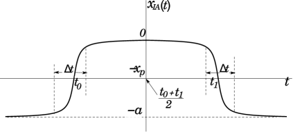
Figure 3: Instanton/anti-instanton pair trajectory in the potential $-V^{(0)}(x)$.

The classical action is computed by replacing Eq. (42) into Eq. (32) and integrating in time between $t_{i}=-t/2$ and $t_{f}=t/2$. We find

$$S_{IA}(t,t_{0}, t_{1})=(V_{0}-V_{a})(t_{1}-t_{0})+V_{a}t$$ (43)

$$-\frac{x^{2}_{p}(V^{\prime\prime}_{0})^{1/2}}{g_{0}}e^{g_{0}(V^{\prime\prime}_{0})^{1/2}(t_{0}-t_{1}+2\Delta_{0p})}$$

$$+U_{\rm eq}(0)-U_{\rm eq}(a)+\sigma^{2}\ln\left|\frac{U^{\prime\prime}_{\rm eq}(a)\;g^{2}_{a}\;(x_{p}+a)}{U^{\prime\prime}_{\rm eq}(0)\;g_{0}^{2}\;x_{p}}\right|$$

$$+\frac{\sigma^{2}}{2}\left[g_{a}^{2}U^{\prime\prime}_{\rm eq}(a)\Delta_{pa}+g_{0}^{2}U^{\prime\prime}_{\rm eq}(0)\Delta_{0p}\right],$$

where we have used the notation $S_{IA}=S_{cl}[x_{IA}]$, i.e., the classical action computed at the instanton/anti-instanton configuration of Eq. (42).

The next step is to compute fluctuations around the instanton/anti-instanton solution. After the time reparametrization given by Eq. (26), we are lead to the computation of the determinant $\det\hat{\Sigma}(\tau_{f},\tau_{i})$, where the operator $\hat{\Sigma}$ is given by Eq. (27), evaluated at $x_{cl}=x_{IA}(\tau)$. Due to time translation invariance, the determinant has zero modes. Similarly to the original computation of instanton fluctuations Coleman (1979), we need to properly take into account translation modes, identifying translation fluctuations with the integration over the collective variables $t_{0}$ and $t_{1}$. We obtain (see Appendix A),

$$K^{(1)}\left(-a,\frac{t}{2}\Big{|}-a,-\frac{t}{2}\right)={\cal N}\int^{t/2}_{-t/2}dt_{0}\int^{t/2}_{t_{0}}dt_{1}\;\times$$ (44)

$$g_{a}\sqrt{S_{I}}g_{0}\sqrt{S_{A}}\;\left[{\det}^{\prime}{\hat{\Sigma}\left(\tau_{f},\tau_{i}\right)}\right]^{-1/2}e^{-\frac{1}{\sigma^{2}}S_{{}_{IA}}(t,t_{0},t_{1})}$$

where $S_{I}=S_{cl}[x_{I}]$, $S_{A}=S_{cl}[x_{A}]$ and the prime in the determinant indicates that it should be evaluated excluding the zero modes. We use the notation $K^{(1)}$ to indicate the contribution of the path $-a\to 0\to-a$ to the propagator. This result is similar to the additive noise case Caroli et al. (1981). The main difference is that the determinant is computed in a reparametrized time and the integration over collective variables $t_{0}$ and $t_{1}$ are renormalized by the diffusion function. The advantage of the reparametrized time is that the operator $\hat{\Sigma}$ has the simpler form of Eq. (27) and can be computed using the Gelfand-Yaglom theorem Dunne (2008). At the end of the calculation, we go back to the original time axes. Following tedious but usual procedures, we finally find

$$K^{(1)}\left(-a,\frac{t}{2}\Big{|}-a,-\frac{t}{2}\right)=-g_{0}^{2}t\;K^{(0)}\;\Gamma\ ,$$ (45)

where $K^{(0)}$ is the contribution of the constant solution, given by Eq. (31), and

$$\Gamma=\frac{\left(U^{\prime\prime}_{\rm eq}(a)|U^{\prime\prime}_{\rm eq}(0)|\right)^{1/2}}{2\pi}\exp\left\{-\frac{U_{\rm eq}(0)-U_{\rm eq}(a)}{\sigma^{2}}\right\}\;.$$ (46)

We see that the contribution of an instanton/anti-instanton configuration to the propagator at long times, is a linear function of time. The structure of the coefficient $\Gamma$ is very interesting. All the information about the stochastic calculus is hidden in the definition of the equilibrium potential, $U_{\rm eq}$. On the other hand, it does not depend on the details of $U_{\rm eq}(x)$, but instead, it depends on the barrier height, $U_{\rm eq}(a)-U_{\rm eq}(0)$, and on the curvature at each maxima, $U^{\prime\prime}_{\rm eq}(0)$ and $U^{\prime\prime}_{\rm eq}(a)$. These properties are quite similar with the additive noise case, except for the fact that the original potential $U(x)$ is replaced by the equilibrium potential $U_{\rm eq}$ and the time is rescaled by the diffusion function at the maximum of the potential $t\to g^{2}_{0}t$. In this way, $K^{(1)}$ does not depend on the details of $g(x)$, but only on its value at the maxima, $g(0)$ and $g(a)$.

Due to the structure of the potential $-V(x)$, there are other trajectories which contribute in a nontrivial way to the propagator; for instance, trajectories that begin in $x=-a$, go to $x=a$ passing through $x=0$, and return to $x=-a$. This kind of trajectories contains two instantons and two anti-instantons as shown in Figure 4.

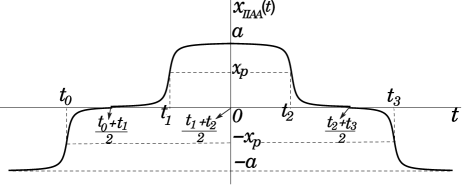
Figure 4: Representation of a trajectory of 2-Instanton and 2-Anti-instanton in the potential $-V^{(0)}(x)$.

The contribution of these trajectories to the propagator can be computed following the same steps of the computation of the single instanton/anti-instanton case. We find, in this case,

$$K^{(2)}\left(-a,\frac{t}{2}\Big{|}-a,-\frac{t}{2}\right)=\frac{(g_{0}^{2}t)^{2}}{2!}\;K^{(0)}\;\Gamma^{2}\ .$$ (47)

Thus, trajectories of the type $-a\to a\to-a$, produce a quadratic time contribution, the coefficient is simply $\Gamma^{2}$, where $\Gamma$ is given by Eq. (46).

V.2 Kramers’ escape rate and time reversal transformation

To compute the conditional probability of remaining in a minimum after some time $t$, we need to sum up all the trajectories that begin and end at $x=-a$ and which contribute to the propagator in a nontrivial way. Having in mind that $\Delta U_{\rm eq}=0$, this probability coincides with the propagator, $P\left(-a,t/2|-a,-t/2\right)=K\left(-a,t/2|-a,-t/2\right)$. As described above, there are essentially three contributions to these paths: a constant one, $K^{(0)}$, given by Eq. (31), a linear term $K^{(1)}$ given by Eq. (45), corresponding to trajectories $-a\to 0\to-a$ or, by symmetry, to $a\to 0\to a$, and, finally, a quadratic term $K^{(2)}$ given by Eq. (47), related to the path $-a\to a\to-a$.

Consider, for instance, a general trajectory containing $\ell_{1}$ paths of the type $-a\to 0\to-a$ and $\ell_{2}$ paths of the type $a\to 0\to a$, related with the linear function $K^{(1)}$. In addition, we allow $m$ paths of the type $-a\to a\to-a$, related with $K^{(2)}$. Then, this particular trajectory will contribute to the propagator with a term

$$K^{(\ell_{1},\ell_{2},m)} \left(-a,\frac{t}{2}\Big{|}-a,-\frac{t}{2}\right)=$$

$$\hskip 28.45274ptK^{(0)}\frac{(-g_{0}^{2}t)^{\ell_{1}+\ell_{2}+2m}}{(\ell_{1}+\ell_{2}+2m)!}\Gamma^{\ell_{1}+\ell_{2}+2m}\ .$$ (48)

By carefully counting the number of different paths which contribute to each trajectory labeled by $(\ell_{1},\ell_{2},m)$ and summing up, we finally arrive at the expression for the conditional probability,

$$P\left(-a,\frac{t}{2}\Big{|}-a,-\frac{t}{2}\right)=\frac{1}{2}K^{(0)}\times\big{(}1+e^{-t/\tau_{k}}\big{)}\;.$$ (49)

On the other hand, by using the same formalism, we easily find the expression for the conditional probability of finding the system in the state $x=a$ at time $t/2$, provided it was in the state $x=-a$ at a previous time $-t/2$,

$$P\left(a,\frac{t}{2}\Big{|}-a,-\frac{t}{2}\right)=\frac{1}{2}K^{(0)}\times\big{(}1-e^{-t/\tau_{k}}\big{)}\;.$$ (50)

In Eqs. (49) and (50), the inverse time parameter $\tau_{k}^{-1}$, which is equivalent to the Kramers’ escape rate, is given by $\tau_{k}^{-1}=r_{\rm mult}=g_{0}^{2}\Gamma$. Using Eq. (46), it is explicitly written as

$$r_{\rm mult}=g_{0}^{2}\frac{\sqrt{U^{\prime\prime}_{\rm eq}(a)|U^{\prime\prime}_{\rm eq}(0)|}}{2\pi}\;e^{-\frac{\Delta U_{\rm eq}}{\sigma^{2}}}\ ,$$ (51)

with $\Delta U_{\rm eq}=U_{\rm eq}(0)-U_{\rm eq}(a)$.

This is one of the main results of our paper. Comparing Eq. (51) with the classical result of Eq. (1), we clearly see the effect of the multiplicative noise. Notice that the role of the original potential $U(x)$ is now played by the equilibrium potential $U_{\rm eq}(x)$ given by Eq. (7). This potential depends not only on the diffusion function $g(x)$ and the noise, but also on the stochastic prescription $\alpha$ which defines the original Langevin equation. There is also an important global scaling factor given by $g^{2}(0)$.

It is worth to mention that, to the best of our knowledge, there are only few papers where analytic expressions for the escape rate in the multiplicative noise case were in fact derived. Indeed, there is no one where different stochastic prescriptions are discussed. In Refs. Jin et al., 2005; Guo and Cheng, 2011; Li-Juan and Wei, 2006, particular examples combining multiplicative with additive noise were treated. There seems to be a consensus that in the exponential part of the Arrhenius form, the classical potential should be replaced by an effective potential computed from the static solution of the Fokker-Planck equation. However, the values presented for the prefactor differ from ours. As a matter of facts, in all that references, there is no indication of the discretization prescription used. This fact is quite important in multiplicative noise, since different prescriptions correspond to completely different stochastic processes. In such a situation, it is necessary to proceed with great care in order to compare analytic expressions and numerical data. In Ref. Rosas et al., 2016, a careful treatment of the first time passage was made by focusing on the Fokker-Planck equation in the Stratonovich prescription. Its result coincides with ours for $\alpha=1/2$ in the weak noise limit.

In order to gain more insight on Eq. (51), let us compare the Kramers’ escape rate with the expression of $r_{\rm mult}$. Expanding Eq. (51) for weak noise. We obtain

$$\frac{r_{\rm mult}}{r_{\rm add}}=|g_{0}|^{2\alpha}|g_{a}|^{2(1-\alpha)}\left(1+O(\sigma^{2})\right)\;.$$ (52)

It can be noticed that the relation between both escape rates does not depend on details of $g(x)$, but on its value at each maxima of $-V(x)$, $x=\pm a$ and $x=0$. As expected, Eq. (52) depends on the stochastic prescription parameter $\alpha$. For instance, in the case of the Stratonovich prescription, $\alpha=1/2$, $r_{\rm mult}/r_{\rm add}=g_{0}g_{a}$. In this case, $g_{0}$ and $g_{a}$ have the same weight. On the other hand, in the Itô interpretation $\alpha=0$, $r_{\rm mult}/r_{\rm add}=g_{a}^{2}$ while, in the thermal prescription, $\alpha=1$, $r_{\rm mult}/r_{\rm add}=g_{0}^{2}$. Indeed, Eq. (52) is invariant under the transformation

$$\alpha \longleftrightarrow 1-\alpha$$ (53)

$$0 \longleftrightarrow a$$ (54)

which is nothing but a time reversal transformation Arenas and Barci (2012b). The simplest way to understand this symmetry is by noting that the instanton solution $x_{I}(t)$ interpolates between the states $x=-a$ and $x=0$. The time reversal solution, the anti-instanton $x_{A}(t)=x_{I}(-t)$, makes the inverse trajectory, i.e., connecting $x=0$ with $x=a$. However, if the forward time process evolves with the $\alpha$ prescription, the backward evolution takes place with the $1-\alpha$ prescription. In this sense, one process is the time reversal conjugate of the other one. For this reason, the kinetic prescription $\alpha=1$ is also called the anti-Itô interpretation. In fact, the only time reversal invariant prescription is the Stratonovich one, $\alpha=1/2$. For details on the time reversal transformation in multiplicative noise dynamics, please see Refs. Arenas and Barci (2012a, b); Moreno et al. (2015).

Let us finally mention that the escape rate in the multiplicative case may be greater or lower than in the additive case, depending essentially on the values of $g(0)$ and $g(a)$. Moreover, if the diffusion function $g(x)$ locally approaches zero at either $x=a$ or $x=0$, the escape rate goes to zero. This effect can be understood from the fact that the effective curvature of $V(x)$ approaches zero and the particle tends to remain in the well for a long time. Of course, our approximation $t\gg\tau_{k}$ is no longer valid in this limit.

VI Numerical simulations

In this section, we perform numerical simulations for the stochastic process driven by the Langevin equation (4) with (5), interpreted in the generalized Stratonovich prescription. We use the Euler-Maruyama scheme, which is the simplest algorithm for this task. This algorithm implies an Itô discretization of the stochastic differential equation (SDE). Thus, for a Langevin equation interpreted in a given $\alpha$ prescription, $0\leq\alpha\leq 1$, it must be transformed to Itô prescription by appropriately changing the drift function $f(x)$. As a consequence, we represent any $\alpha$ defined SDE by means of the following Itô differential equation,

$$\frac{dx}{dt}=-\frac{1}{2}g^{2}(x)\frac{dU(x)}{dx}+\sigma^{2}\alpha g(x)g^{\prime}(x)+g(x)\eta(t).$$ (55)

Eq. (55) was obtained from Eq. (4) by shifting $f(x)\to f(x)+\sigma^{2}\alpha g(x)g^{\prime}(x)$ Moreno et al. (2019).

Considering the model given by Eqs. (8) and (9), we explicitly have the Itô SDE,

$$dx= \frac{x\left(1+\lambda x^{2}\right)}{2}\left\{\left(1-x^{2}\right)\left(1+\lambda x^{2}\right)+4\lambda\sigma^{2}\alpha\right\}dt$$

$$+\left(1+\lambda x^{2}\right)dW\;,$$ (56)

where $W(t)$ is a standard Wiener process with $\langle W(t)\rangle=0$ and $\langle W(t)W(t^{\prime})\rangle=\sigma^{2}{\rm min}(t,t^{\prime})$. In Figure 5, we show a typical output for a particular noise realization.

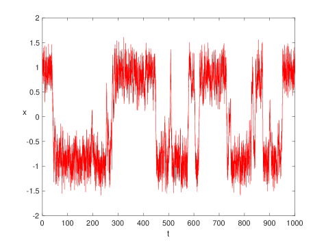
Figure 5: $x(t)$, computed from the integration of Eq. (56) for a particular realization of the noise, for $\lambda=0.5$, $\alpha=1/2$ and $\sigma^{2}=0.095$. Time interval $0<t<1000$ was divided into $2\times 10^{4}$ steps.

Fixing the initial condition $x(0)=1$, we clearly see the dynamics of the stochastic variable $x(t)$, fluctuating around the potential minima $x_{\rm min}\sim\pm 1$, flipping between them at seemly irregular times.

We have computed the mean value $\langle x(t)\rangle$ over different noise realizations. In Figure 6, we show the result of averaging over $8\times 10^{4}$ configurations of the noise for different values of the stochastic prescription.

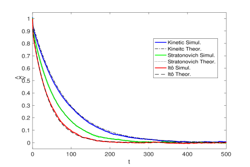
Figure 6: $\langle x(t)\rangle$ averaged over $8\times 10^{4}$ noise realizations. We fixed the initial condition $x(0)=1$ and the parameters $\lambda=0.5$ and $\sigma^{2}=0.085$. The three curves corresponds to three different stochastic prescriptions, $\alpha=0,1/2,1$. The continuous lines are the numerical simulations while the dashed, dot and dashed-dot lines correspond to a theoretical fitting using Eq. (51), in the Itô, Stratonovich and Kinetics stochastic prescription, respectively.

We can observe that, as expected, $\langle x(t)\rangle$ tends to zero exponentially. This means that, at long times, the particle is flipping between both potential wells with zero mean value. We can also observe that the typical decay time is not the same for different stochastic prescriptions and, in general, $\tau_{I}<\tau_{S}<\tau_{K}$, where $\tau_{I}$, $\tau_{S}$ and $\tau_{K}$ are the decay times in the Itô, Stratonovich and Kinetic prescriptions. This is consistent with the fact observed in Figure 1, where we can see that the height of the equilibrium potential barrier increases with increasing $\alpha$.

By using the asymptotic conditional probability distributions, Eqs. (49) and (50), it is not difficult to show that, for $t>>\tau_{k}$,

$$\langle x(t)\rangle=A\;e^{-t/\tau_{k}},$$ (57)

where $A$ is some constant. We have used Eq. (57), with $\tau_{k}=r_{\rm mult}^{-1}$ computed in Eq. (51), to compare the simulations and the theoretical prediction in the three cases shown in Figure 6, obtaining excellent fittings.

In order to have more accurate results, the numerical decay rate $r=\tau^{-1}_{k}$ can be obtained from a linear least-square fitting of $\ln\langle x(t)\rangle$. Following this procedure, we studied a wide range of the parameter space $\{\alpha,\sigma^{2}\}$ and we compared the output with the analytic decay rate of Eq. (51). In Figure 7, we show the decay rate $r_{\rm mult}$ as a function of the noise intensity $\sigma^{2}$ for three different values of the stochastic prescription.

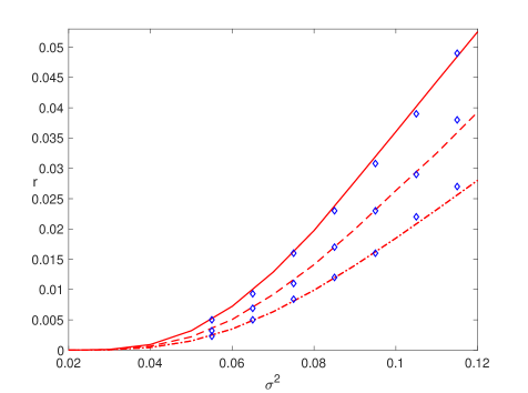
Figure 7: Decay rate $r_{mult}$ as a function of the noise intensity $\sigma^{2}$ computed using Eq. (51). The continuous line corresponds to the decay rate in the Itô prescription. For Stratonovich and kinetic or anti-Itô interpretation, the decay rate is depicted by the dashed and dot-dashed curves, respectively. The points (diamonds) were obtained from a linear fitting of $\ln\langle x(t)\rangle$ through numerical simulations for each case. For all the data, it was fixed $\lambda=0.5$.

The continuous line represents the decay rate in the Itô prescription. The Stratonovich interpretation is depicted by the dashed line and the dot-dashed curve shows the decay rate in the Kinetic or anti-Itô prescription. The diamonds are numerical results obtained by the least-square fitting of $\ln\langle x(t)\rangle$ in each case. We can observe an excellent agreement over almost all the noise range. As expected, there is a small deviation for larger values of the noise, since in these cases $\Delta U_{\rm eq}/\sigma^{2}\gtrsim 1$, and the Arrhenius form is no longer a good approximation.

In Figure 8 we show the decay rate $r_{\rm mult}$ as a function of the stochastic prescription $0\leq\alpha\leq 1$, for different values of the noise from $\sigma^{2}=0.055$ to $\sigma^{2}=0.085$.

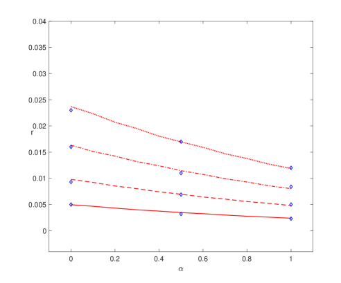
Figure 8: Decay rate $r=\tau_{k}^{-1}$ as a function of the stochastic prescription $\alpha$ obtained from Eq. (51) for different values of $\sigma^{2}$. The continuous line is plotted for $\sigma^{2}=0.055$, dashed line corresponds to $\sigma^{2}=0.065$, while the dot-dashed and dotted lines correspond to $\sigma^{2}=0.075$ and $\sigma^{2}=0.085$, respectively. The points (diamonds) results from numerical simulation, computed by linear fittings of $\ln\langle x(t)\rangle$. Parameter $\lambda=0.5$ was fixed for all the curves.

We observe an excellent agreement between the theoretical predictions and the data computed from the numerical simulation of the Langevin equation. In this figure, the continuous line was plotted fixing $\sigma^{2}=0.055$ and has a perfect match with the numerical results. We expect that lower values of the noise produce still better results. However, for these values, the time decays are huge, being on the order of $t=1000$ for $\sigma^{2}=0.055$. So, in order to have statistics for a lower noise range, it would be necessary to simulate for very longer times scales considering a big number of noise realizations. Of course, this consumes much more computational resources.

VII Summary and conclusions

We have considered the problem of a particle in a symmetric double-well potential $U(x)$, with a dynamics driven by an overdamped multiplicative Langevin equation characterized by a symmetric diffusion function $g(x)=g(-x)$. The stochastic differential equation was defined in the generalized Stratonovich prescription, parametrized by a continuum parameter $0\leq\alpha\leq 1$. This prescription contains the usual stochastic interpretations for particular values of the parameter $\alpha$. Indeed, $\alpha=0,1/2,1$ corresponds to the usual Itô, Stratonovich and Kinetic prescriptions, respectively.

We have provided a path integral technique to compute conditional probabilities in the weak noise approximation for arbitrary values of the parameter $\alpha$. Interestingly, all the dependence of $\alpha$ is codified in the equilibrium potential $U_{\rm eq}(x)$, obtained by means of a static solution of the associated Fokker-Planck equation.

It was introduced a local time reparametrization, which allows to exactly integrate fluctuations around saddle-point solutions. Conditional probabilities were computed for long time intervals by generalizing the instanton/anti-instanton diluted gas approximation, already developed for the additive noise case Caroli et al. (1981). From these probabilities, the escape rate was computed in the same approximation and the result was compared with the Kramers’ escape rate for additive noise dynamics.

The main result of the paper is given by Eq. (51). We found that the general structure of the escape rate keeps the Arrhenius form of the Kramers’ result. The main corrections are twofold. First, the equilibrium potential $U_{\rm eq}(x)$ of Eq. (7) plays the role of the bare potential $U(x)$. The potential $U_{\rm eq}(x)$ is generally different from $U(x)$ in the multiplicative noise case, depending on the diffusion function and the stochastic prescription $\alpha$. Indeed, the only stochastic prescription in which $U_{\rm eq}(x)=U(x)$ is the anti-Itô prescription $\alpha=1$. Moreover, there is a global scale factor $g^{2}(0)$ that has its origin in the time reparametrization necessary to correctly compute fluctuations.

In the weak noise limit, we found a simple relation between the Kramers’ escape rates computed with additive and multiplicative noise, given by Eq. (52). The obvious consistency check is that $r_{\rm mult}/r_{\rm add}=1$ in the limit $g(x)\to 1$ (or $\lambda\to 0$ in the particular example). In addition, we observe that $g(0)$ and $g(a)$ enter with different weights depending on the prescription parameter $\alpha$. These weights are consistent with a time reversal transformation, which relates a stochastic process in the $\alpha$ prescription with its time reversal conjugate $1-\alpha$. Indeed, the Stratonovich convention $\alpha=1/2$ is the only one with time reversal invariance and, in this case, both maxima enter with the same weight.

Finally, we have made extensive Langevin simulations to test the accuracy of our expressions. We have explored a huge region of the parameter space $\{\sigma,\alpha\}$, in which the high barrier approximation, $\Delta U_{\rm eq}/\sigma^{2}>>1$, is well defined. We have found a very good agreement for all values of the stochastic prescription.

Although we have presented results for a system with full reflection symmetry $x\to-x$, the methods developed in this paper are completely general. We hope to communicate results for a more general non-symmetric case in the near future. Moreover, having analytic expressions for the conditional probability we can face the problem of stochastic resonance in multiplicative noise processes in a more solid bases.

Appendix A Zero modes in the multiplicative case

The relation of zero modes of the fluctuation operator and translation invariance is very well known in quantum mechanics Coleman (1979), as well as in additive noise stochastic dynamics Caroli et al. (1981). In this appendix, we focus on the effect produced by the diffusion function $g(x)$ in a multiplicative noise stochastic system.

Let us consider the instanton function $x_{I}(t)$ as a solution of the equation of motion Eq. (17), with boundary conditions $\lim_{t\to-\infty}x_{I}(t)=-a$ and $\lim_{t\to\infty}x_{I}(t)=0$, where $-a$ and $0$ are the positions of a minimum and the local maximun of $U_{\rm eq}(x)$, respectively. In the weak noise approximation, these values coincide with two local maxima of $-V(x)$ as shown in Figure 2. It is not difficult to show that $dx_{I}/dt$ is a zero mode of the fluctuation operator Eq. (24). To see this, we consider

$$\int dt^{\prime}O(t,t^{\prime}) \frac{dx_{I}(t^{\prime})}{dt^{\prime}}=$$ (58)

$$-\frac{d}{dt}\left(\frac{1}{g^{2}}\frac{d^{2}x_{I}}{dt^{2}}\right)+\left(\frac{1}{g^{2}}V^{\prime}_{\rm eff}\right)^{\prime}\frac{dx_{I}}{dt}=$$

$$-\frac{d}{dt}\left(\frac{1}{g^{2}}V^{\prime}_{\rm eff}\right)+\left(\frac{1}{g^{2}}V^{\prime}_{\rm eff}\right)^{\prime}\frac{dx_{I}}{dt}=0$$

where in the first term of the last line we have used $d^{2}x_{I}/dt^{2}=V_{\rm eff}$ and in the second term we used the chain rule.

Thus, the fluctuation operator has a normalized zero mode of the form

$$\eta_{0}(t)=A\frac{dx_{I}(t)}{dt}\ ,$$ (59)

where $A$ is a normalization constant. To determine it, we impose,

$$\int dt\;\eta_{0}^{2}(t)=A^{2}\int dt\;\left(\frac{dx_{I}}{dt}\right)^{2}=1$$ (60)

and, thus, the normalization constant reads

$$A^{-2}=\int dt\;\left(\frac{dx_{I}}{dt}\right)^{2}.$$ (61)

The action computed at the instanton solution is

$$S_{I}=\int dt\left\{\frac{1}{2g^{2}(x_{I})}\left(\frac{dx_{I}}{dt}\right)^{2}+V(x_{I})\right\}.$$ (62)

Using the equations of motion, it can be written as

$$S_{I}=\int dt\;\frac{1}{g^{2}(x_{I})}\left(\frac{dx_{I}}{dt}\right)^{2}.$$ (63)

Since the zero mode has a small support around $t_{0}$, in the thin-wall approximation we can write with good accuracy

$$S_{I}\sim\frac{1}{g^{2}_{a}}\int dt\left(\frac{dx_{I}}{dt}\right)^{2},$$ (64)

where $g_{a}=g(a)$. Replacing this result in Eq. (61) we finally find the normalized zero mode

$$\eta_{0}(t)=\frac{1}{g_{a}\sqrt{S_{I}}}\frac{dx_{I}(t)}{dt}.$$ (65)

In order to compute fluctuations, we perform a local time reparametrization given by Eq. (26). We are lead to the computation of the integral

$$I_{F}=\int[{\cal D}\delta x]\;e^{-\frac{1}{2}\int d\tau\delta x(\tau)\left(-\frac{d^{2}~{}}{d\tau^{2}}+W[x_{cl}]\right)\delta x(\tau)}\ ,$$ (66)

where $W$ is given by Eq. (28). To compute it, we expand fluctuations in eigenfunctions of the fluctuation operator, taking special care with the translational modes that are responsible for the zero mode. We write the fluctuation field in the following form

$$\delta x(\tau)=c_{0}\psi_{0}(\tau-\tau_{0})+\sum_{k=1}^{\infty}c_{k}\psi_{k}(\tau-\tau_{0}),$$ (67)

where $\psi_{k}$ are eigenvectors

$$\left(-\frac{d^{2}~{}}{d\tau^{2}}+W[x_{cl}]\right)\psi_{n}(\tau)=\lambda_{n}\psi_{n}(\tau)$$ (68)

with eigenvalues $\lambda_{k}\neq 0$ and the zero mode in the reparametrized variable reads

$$\psi_{0}(\tau)=\frac{1}{g_{a}\sqrt{S_{I}}}\;g^{2}(x_{I}(\tau))\frac{dx_{I}(\tau)}{d\tau}\;.$$ (69)

The functional measure can be written in terms of the coefficients $c_{k}$ as

$${\cal D}\delta x=dc_{0}\prod_{k\neq 0}dc_{k}\ .$$ (70)

Computing the variation of fluctuations under time translation, we have that

$$d\delta x(\tau)=\frac{dx_{I}}{d\tau}d\tau_{0}\ .$$ (71)

On the other hand, a variation in the zero mode reads

$$d\delta x(\tau)=\frac{1}{g_{a}\sqrt{S_{I}}}\;g^{2}(x_{I}(\tau))\frac{dx_{I}}{d\tau}dc_{0}\ .$$ (72)

Now, comparing Eqs. (71) and (72) and using the reparametrization identity $d\tau/dt=g^{2}(x_{I})$, we immediately find

$$dc_{0}=g_{a}\sqrt{S_{I}}dt_{0}\ .$$ (73)

In this way,

$$I_{F} =\int g_{a}\sqrt{S_{I}}dt_{0}\int\left(\prod_{k\neq 0}dc_{k}\right)\exp\left(-\frac{1}{2}\sum_{n}\lambda_{n}(\tau_{0})c_{n}^{2}\right)$$

$$=\int g_{a}\sqrt{S_{I}}dt_{0}\left(\prod_{k\neq 0}\lambda_{k}^{-1/2}(\tau_{0})\right)$$

$$=\int dt_{0}\;g_{a}\sqrt{S_{I}}\;\left({\det}^{\prime}\left(-\frac{d^{2}~{}}{d\tau^{2}}+W[x_{cl}]\right)\right)^{-1/2}$$ (74)

where the prime means that the determinant should be computed without the zero mode.

Thus, the usual interpretation of the zero mode as an integration in the collective variable $dt_{0}$ is still valid in the multiplicative case. However, the constant of proportionality is renormalized by the diffusion function $g_{a}$, computed at the minimum of the potential.

The same reasoning applies to the anti-instanton solutions. However, in this case, the variation is proportional to $g_{0}\sqrt{S_{A}}dt_{1}$, where $g_{0}$ is evaluated at the maximum of the potential and $S_{A}$ is the classical action evaluated at the anti-instanton solution. This analysis leads to Eq. (44) for $K^{(1)}$.

References

- Fleming and Hänggi (1993) G. R. Fleming and P. Hänggi, Activated Barrier Crossing: Applications In Physics, Chemistry And Biology, Advanced Database Research and Development Series (World Scientific Publishing Company, Singapore, 1993).
- Kramers (1940) H. Kramers, Physica 7, 284 (1940).
- Hänggi et al. (1990) P. Hänggi, P. Talkner, and M. Borkovec, Rev. Mod. Phys. 62, 251 (1990).
- Bray and McKane (1989) A. J. Bray and A. J. McKane, Phys. Rev. Lett. 62, 493 (1989).
- McKane et al. (1990) A. J. McKane, H. C. Luckock, and A. J. Bray, Phys. Rev. A 41, 644 (1990).
- Bray et al. (1990) A. J. Bray, A. J. McKane, and T. J. Newman, Phys. Rev. A 41, 657 (1990).
- Luckock and McKane (1990) H. C. Luckock and A. J. McKane, Phys. Rev. A 42, 1982 (1990).
- Jung et al. (2005) P. Jung, A. Neiman, M. K. N. Afghan, S. Nadkarni, and G. Ullah, New Journal of Physics 7, 17 (2005).
- Goulding et al. (2007) D. Goulding, S. Melnik, D. Curtin, T. Piwonski, J. Houlihan, J. P. Gleeson, and G. Huyet, Phys. Rev. E 76, 031128 (2007).
- Lançon et al. (2001) P. Lançon, G. Batrouni, L. Lobry, and N. Ostrowsky, EPL (Europhysics Letters) 54, 28 (2001).
- Lançon et al. (2002) P. Lançon, G. Batrouni, L. Lobry, and N. Ostrowsky, Physica A: Statistical Mechanics and its Applications 304, 65 (2002).
- Lau and Lubensky (2007) A. W. C. Lau and T. C. Lubensky, Phys. Rev. E 76, 011123 (2007).
- Volpe et al. (2010) G. Volpe, L. Helden, T. Brettschneider, J. Wehr, and C. Bechinger, Phys. Rev. Lett. 104, 170602 (2010).
- Brettschneider et al. (2011) T. Brettschneider, G. Volpe, L. Helden, J. Wehr, and C. Bechinger, Phys. Rev. E 83, 041113 (2011).
- García-Palacios and Lázaro (1998) J. L. García-Palacios and F. J. Lázaro, Phys. Rev. B 58, 14937 (1998).
- Aron et al. (2014) C. Aron, D. G. Barci, L. F. Cugliandolo, Z. G. Arenas, and G. S. Lozano, Journal of Statistical Mechanics: Theory and Experiment 2014, P09008 (2014).
- Arenas et al. (2018) G. Arenas, D. G. Barci, and M. V. Moreno, Physica A: Statistical Mechanics and its Applications 510, 98 (2018).
- Hinrichsen (2000) H. Hinrichsen, Advances in Physics 49, 815 (2000), https://doi.org/10.1080/00018730050198152 .
- Van den Broeck et al. (1994) C. Van den Broeck, J. M. R. Parrondo, and R. Toral, Phys. Rev. Lett. 73, 3395 (1994).
- Castro et al. (1995) F. Castro, A. D. Sánchez, and H. S. Wio, Phys. Rev. Lett. 75, 1691 (1995).
- Carrillo et al. (2003) O. Carrillo, M. Ibañes, J. García-Ojalvo, J. Casademunt, and J. M. Sancho, Phys. Rev. E 67, 046110 (2003).
- Jafarpour et al. (2015) F. Jafarpour, T. Biancalani, and N. Goldenfeld, Phys. Rev. Lett. 115, 158101 (2015).
- Barci et al. (2016) D. G. Barci, Z. G. Arenas, and M. V. Moreno, EPL (Europhysics Letters) 113, 10009 (2016).
- Benzi et al. (1981) R. Benzi, A. Sutera, and A. Vulpiani, Journal of Physics A: Mathematical and General 14, L453 (1981).
- Benzi et al. (1983) R. Benzi, G. Parisi, A. Sutera, and A. Vulpiani, SIAM Journal on Applied Mathematics 43, 565 (1983), https://doi.org/10.1137/0143037 .
- Wio, H. S. and Deza, R. R. (2007) Wio, H. S. and Deza, R. R., Eur. Phys. J. Special Topics 146, 111 (2007).
- Wio et al. (2002) H. Wio, S. Bouzat, and B. von Haeften, Physica A: Statistical Mechanics and its Applications 306, 140 (2002), invited Papers from the 21th {IUPAP} International Conference on St atistical Physics.
- Jin et al. (2005) Y. Jin, W. Xu, and M. Xu, Chaos, Solitons & Fractals 26, 1183 (2005).
- Guo and Cheng (2011) F. Guo and X.-F. Cheng, J. Korean Phy. Soc. 58, 1567 (2011).
- Li-Juan and Wei (2006) N. Li-Juan and X. Wei, Chinese Physics Letters 23, 3180 (2006).
- Zheng et al. (2011) X.-D. Zheng, X.-Q. Yang, and Y. Tao, PLOS ONE 6, 1 (2011).
- Rosas et al. (2016) A. Rosas, I. L. D. Pinto, and K. Lindenberg, Phys. Rev. E 94, 012101 (2016).
- Sivak et al. (2013) D. A. Sivak, J. D. Chodera, and G. E. Crooks, Phys. Rev. X 3, 011007 (2013).
- Goldenfeld (1992) N. Goldenfeld, Lectures On Phase Transitions And The Renormalization Group (Frontiers in Physics v.85, Perseus Books Publishing L.L.C., New York, USA, 1992).
- Wio (2013) H. Wio, Path Integrals for Stochastic Processes: An Introduction (World Scientific, 2013).
- Aron et al. (2010) C. Aron, G. Biroli, and L. F. Cugliandolo, Journal of Statistical Mechanics: Theory and Experiment 2010, P11018 (2010).
- Arenas and Barci (2010) Z. G. Arenas and D. G. Barci, Phys. Rev. E 81, 051113 (2010).
- Arenas and Barci (2012a) Z. G. Arenas and D. G. Barci, Phys. Rev. E 85, 041122 (2012a).
- Arenas and Barci (2012b) Z. G. Arenas and D. G. Barci, Journal of Statistical Mechanics: Theory and Experiment 2012, P12005 (2012b).
- Moreno et al. (2015) M. V. Moreno, Z. G. Arenas, and D. G. Barci, Phys. Rev. E 91, 042103 (2015).
- Aron et al. (2016) C. Aron, D. G. Barci, L. F. Cugliandolo, Z. G. Arenas, and G. S. Lozano, Journal of Statistical Mechanics: Theory and Experiment 2016, 053207 (2016).
- Janssen (1992) H. K. Janssen, From phase transitions to chaos: Topics in Modern Statistical Physics (World Scientific, Singapore, 1992).
- Moreno et al. (2019) M. V. Moreno, D. G. Barci, and Z. G. Arenas, Phys. Rev. E 99, 032125 (2019).
- Zinn-Justin (2002) J. Zinn-Justin, Quantum field theory and critical phenomena (Oxford University Press, USA, 2002).
- Coleman (1979) S. Coleman, “The uses of instantons,” in The Whys of Subnuclear Physics, edited by A. Zichichi (Springer US, Boston, MA, 1979) pp. 805–941.
- Caroli et al. (1979) B. Caroli, C. Caroli, and B. Roulet, Journal of Statistical Physics 21, 415 (1979).
- Caroli et al. (1981) B. Caroli, C. Caroli, and B. Roulet, Journal of Statistical Physics 26, 83 (1981).
- Hänggi (1978) P. Hänggi, Helv. Phys. Acta 51, 183 (1978).
- Hänggi and Thomas (1982) P. Hänggi and H. Thomas, Phys. Rep. 88, 207 (1982).
- Klimontovich (1994) Y. L. Klimontovich, Physics-Uspekhi 37, 737 (1994).
- Brézin et al. (1977) E. Brézin, G. Parisi, and J. Zinn-Justin, Phys. Rev. D 16, 408 (1977).
- Bogomolny (1980) E. Bogomolny, Physics Letters B 91, 431 (1980).
- Dunne (2008) G. V. Dunne, Journal of Physics A: Mathematical and Theoretical 41, 304006 (2008).