A Caputo based SIRS and SIS fractional order models with standard incidence rate and varying population

Abstract

In the present work, we have introduced and studied two epidemic models that are constructed with Caputo fractional derivative. We considered standard incidence rate and varying population dynamics for SIS and SIRS mathematical models. Model equilibria, basic reproduction numbers are determined and local stability analysis are established for the two fractional dynamical models. Finally, the efficient fracPECE iterative scheme for fractional order deterministic dynamical models is applied to perform numerical simulations.

Keywords: Fractional-order model, Caputo derivative, fracPECE iterative scheme.

1 Introduction

Mathematical models have played role in understanding infectious diseases epidemiology (Hethcote, 2000). Epidemiological models formulated with system of nonlinear fractional order equations have been studied by several authors and it is still gaining a lot of attention in mathematical biology [see, e.g, Qureshi and Atangana (2019), Pinto and Carvalho (2019), Wang et al. (2019), Jajarmi et al. (2019), Ameen and Novati (2017), Rihan et al. (2019), R. Jan et al. (2019), Arafa et al. (2012), Almeida (2018)]. An SEIR compartmental model formulation that describes the dynamical behaviour of an influenza A infection is introduced and analyzed by the authors in (González-Parra et al., 2014) using nonlinear fractional order equations. A co-infection epidemic model for malaria and HIV/AIDS infections with fractional order derivative that captures time delay dynamics is studied (Carvalho and Pinto, 2016). A mathematical model that describes the dynamics of an HIV/AIDS infection using Caputo based fractional derivative is studied (Silva and Torres, 2019).

A Caputo fractional derivative is used to construct a nonlinear epidemic model that captures vertical transmission dynamics (Ozalp and Demirci, 2011). A deterministic model with fractional order formulation is presented to study the dynamical behavior between viral particles, humoral immune response mediated by the antibodies and susceptible host cells (Boukhouima et al., 2018). In the work of (Ahmed and El-Saka, 2010), the authors derived and studied a non-integer order mathematical model for Hepatitis C disease. Carvalho et al. (2018) formulated and analyzed a nonlinear fractional order initial value problem for the co-infection dynamics of Hepatitis C and HIV. A compartmental model for Hepatitis B infection that includes cure of infected cells is presented and analyzed using system of fractional order nonlinear equations (Salman and Yousefl, 2017). A non-standard finite discretization scheme is applied to solve two nonlinear Hepatitis B infection models that are of fractional orders (Ullah et al., 2018). Fractional order deterministic models based on an MSEIR compartmental formulation have recently been introduced in the works done by the authors in (Qureshi and Yusuf, 2019, Almeida et al., 2019)

El-Saka (2014) developed and analyzed an SIS model with bilinear incidence rate and varying populaton dynamics. He formulated the epidemic model using differential equations based on Caputo derivative. The same author in (El-Saka, 2013) introduced a Caputo based SIRS and SIR models with varying populaton dynamics and bilinear incidence rates. A fractional SIS model problem with constant population and standard incidence rate has been introduced and studied in (Hassouna et al., 2018). El-Saka et al. (2019) has derived a fractional order Susceptible-Infected-Recovered-Susceptible (SIRS) model based on homogeneous networks. They applied global stability concepts in the work by (Vargas-De-Leó, 2015) and established global stability for their constructed epidemic model. A fractional dynamical problem has been derived and analyzed for the classic SIR endemic model with constant population size (Okyere et al., 2016). The authors in (Liu et al., 2019) have derived and analyzed an SIS epidemic model based on fractional dynamical nonlinear equations and complex networks. The recent work by the authors in (Mouaouine et al., 2018) deals with mathematical formulation of an SIR model with varying population size, nonlinear incidence and Caputo fractional derivative.

The fractional order formulation approach we consider for the SIS and SIRS models in our present study is motivated by work done in (Diethelm, 2013). The modeling concept introduced in (Diethelm, 2013) has been used by many authors (see, e.g, Carvalho et al., 2018, Sardar et al., 2015, Carvalho and Pinto, 2016, Okyere et al., 2016). In this study, we will modify and analyze an SIS mathematical model introduced in (Vargas-De-Leó, 2015). We will also propose a new SIRS model with fractional order dynamics.

The outline for the rest of the work is organized as follows: Section 2 is concern with some useful preliminaries on fractional calculus. We present the first mathematical model which is based on an SIS compartmental modeling formulation with fractional order dynamics in section 3. We then present an SIRS model with fractional order dynamics in section 4. Local stability analysis, numerical simulations and discussions are presented for the two dynamical models in their respective sections. We then conclude the study in section 5

2 Preliminaries

In this work, our modeling formulation is motivated by well-known Caputo derivative in fractional calculus. Several applications of this fractional derivative in engineering and science have been studied in the text books by the authors in (Petras, 2011, Podlubny, 1999).

Definition 1

(Podlubny, 1999) Fractional integral of order $\alpha$ is defined as

$$I^{\alpha}v(t)=\frac{1}{\Gamma(\alpha)}\int_{0}^{t}\!\frac{v(x)}{(t-x)^{1-\alpha}}\,\mathrm{d}x$$

for $0<\alpha<1,\ t>0.$

Definition 2

(Podlubny, 1999) Caputo fractional derivative of order $\alpha$ is defined as

$$D^{\alpha}v(t)=\frac{1}{\Gamma(m-\alpha)}\int_{0}^{t}\!\frac{v^{m}(x)}{(t-x)^{\alpha+1-m}}\,\mathrm{d}x.$$

for $m-1<\alpha<m.$

3 SIS model with fractional order dynamics

In this section, we modify and study an existing SIS model that is characterised by system of nonlinear fractional order equations with standard incidence rate. This type of deterministic compartmental structure (susceptible-infected-susceptible) is used to study the dynamical behaviour of infections that do not confer immunity. The total population is grouped into two sub-populations namely susceptible individuals, $Q_{S}$ and infected individuals, $Q_{I}$. The fractional order dynamical model presented and analysed in (Vargas-De-Leó, 2015) is given by the nonlinear system as follows,

$$D_{t}^{\alpha}Q_{S}(t) =\Lambda-\dfrac{\varphi Q_{S}Q_{I}}{Q_{S}+Q_{I}}-\nu Q_{S}+\omega Q_{I}$$ (1)

$$D_{t}^{\alpha}Q_{I}(t) =\dfrac{\varphi Q_{S}Q_{I}}{Q_{S}+Q_{I}}-(\eta+\nu+\omega)Q_{I}$$

The positive model parameters which includes $\Lambda,\ \beta,\ \nu,\ \eta$ and $\omega$ represent recruitment rate of susceptible individuals corresponding to births and immigration, infection rate, natural death rate, disease induced death rate and the rate at which infectious individuals return to the susceptible class after infectious period respectively.

From the nonlinear system (1), it is not hard to see that, there is a mismatch of time dimension on both sides of the system of equations. The left-hand side has a time dimension of $(time)^{-\alpha}$ and the time dimension of the right-hand side is $(time)^{-1}$. The fractionalization method introduced and studied in (Diethelm, 2013) rectifies this drawback of time dimension.

Therefore motivated by the modeling approach in (Diethelm, 2013), the new modified epidemic model which is an improved version of the fractional dynamical initial value problem (1) is given by

$$D_{t}^{\alpha}Q_{S}(t) =\Lambda^{\alpha}-\dfrac{\varphi^{\alpha}Q_{S}Q_{I}}{Q_{S}+Q_{I}}-\nu^{\alpha}Q_{S}+\omega^{\alpha}Q_{I}$$ (2)

$$D_{t}^{\alpha}Q_{I}(t) =\dfrac{\varphi^{\alpha}Q_{S}Q_{I}}{Q_{S}+Q_{I}}-(\eta^{\alpha}+\nu^{\alpha}+\omega^{\alpha})Q_{I}$$

Knowing that $N=Q_{S}+Q_{I}$, the fractional differential equation describing the dynamics of the total population is given by

$$D_{t}^{\alpha}N =\Lambda^{\alpha}-\eta^{\alpha}Q_{I}-\nu^{\alpha}N$$ (3)

Since the right-hand side of equation (3) is not equal to zero, it implies that, the total population may vary in time.

3.1 Model equlilibria and local stablility analysis

There are two equilibrium points for the fractional dynamical system (2)
given by $H_{df}=\bigg{(}\dfrac{\Lambda^{\alpha}}{\nu^{\alpha}},0\bigg{)}$ and $H_{en}=\bigg{(}{Q_{S}}^{*},{Q_{I}}^{*}\bigg{)}$

where

$${Q_{S}}^{*} =\dfrac{\Lambda^{\alpha}}{\nu^{\alpha}+\big{(}\eta^{\alpha}+\nu^{\alpha}\big{)}\big{(}R_{0}-1\big{)}};$$

$${Q_{I}}^{*} =\dfrac{\big{(}R_{0}-1\big{)}\Lambda^{\alpha}}{\nu^{\alpha}+\big{(}\eta^{\alpha}+\nu^{\alpha}\big{)}\big{(}R_{0}-1\big{)}}.$$

$H_{df}$ and $H_{en}$ represent disease-free and endemic equilibrium points respectively.

The basic reproduction number $R_{0}$ associated with the model problem (2) is given as

$$R_{0}=\dfrac{\varphi^{\alpha}}{\eta^{\alpha}+\nu^{\alpha}+\omega^{\alpha}}.$$

At the endemic equilibrium, we obtain the following two identities given by

$$\dfrac{\varphi^{\alpha}{Q_{S}}^{*}}{{Q_{S}}^{*}+{Q_{I}}^{*}} =\eta^{\alpha}+\nu^{\alpha}+\omega^{\alpha}$$ (4)

$$\Lambda^{\alpha} =(\eta^{\alpha}+\nu^{\alpha}){Q_{I}}^{*}+\nu^{\alpha}{Q_{I}}^{*}$$ (5)

Theorem 1

The equilibrium point $H_{df}$ (disease-free) of the SIS model (2) is locally asymptotically stable if $R_{0}<1$ and unstable if $R_{0}>1.$

Proof. The Jacobian matrix of the dynamical fractional SIS model (2) computed at $H_{df}$ is given by

$$J(H_{df})=\begin{bmatrix}-\nu^{\alpha}&-\varphi^{\alpha}+\omega^{\alpha}\\ \\ 0&\varphi^{\alpha}-\big{(}\eta^{\alpha}+\nu^{\alpha}+\omega^{\alpha}\big{)}\end{bmatrix}$$

For the equilibrium point $H_{df}$ to be locally asymptotically stable, it is necessary and sufficient to verify that the all the eigenvalues of matrix $J(H_{df})$ satisfy the stability condition derived and analyzed in (Ahmed et al., 2006).

$$\mathinner{\!\left\lvert arg(\lambda_{i})\right\rvert}>\frac{\alpha\pi}{2}$$ (6)

Since the $2\times 2$ matrix $J(H_{df})$ is a diagonal matrix, it is not hard to see that the eigenvalues are $\lambda_{1}=-\nu^{\alpha}<0$ and $\lambda_{2}=\varphi^{\alpha}-\big{(}\eta^{\alpha}+\nu^{\alpha}+\omega^{\alpha}\big{)}$. For the two eigenvalues to satisfy the stability condition (6), it is sufficient to show that $\lambda_{2}$ has negative real part.

$$\lambda_{2} =\varphi^{\alpha}-\big{(}\eta^{\alpha}+\nu^{\alpha}+\omega^{\alpha}\big{)}$$

$$=\big{(}\eta^{\alpha}+\nu^{\alpha}+\omega^{\alpha}\big{)}\bigg{[}\dfrac{\varphi^{\alpha}}{\big{(}\eta^{\alpha}+\nu^{\alpha}+\omega^{\alpha}\big{)}}-1\bigg{]}$$

$$=\big{(}\eta^{\alpha}+\nu^{\alpha}+\omega^{\alpha}\big{)}\big{[}R_{0}-1\big{]}<0\hskip 8.5359ptiff\hskip 8.5359ptR_{0}<0$$

Knowing that $\lambda_{1}=-\nu^{\alpha}<0$ and following the basic manipulations on the second eigenvalue above, we can conclude that both eigenvalues satisfy the stability condition (6).   

Theorem 2

The equilibrium point $H_{en}$ of the SIS model (2) is locally asymptotically stable if $R_{0}>1$.

Proof. The Jacobian matrix of the dynamical fractional SIS model (2) computed at $H_{en}$ is given by

$$J(H_{en})=\begin{bmatrix}-\bigg{(}\nu^{\alpha}+\frac{\varphi^{\alpha}({Q_{I}}^{*})^{2}}{\big{(}{Q_{S}}^{*}+{Q_{I}}^{*}\big{)}^{2}}\bigg{)}&&&\frac{\varphi({Q_{S}}^{*})^{2}}{\big{(}{Q_{S}}^{*}+{Q_{I}}^{*}\big{)}^{2}}+\omega^{\alpha}\\ \\ \\ \frac{\varphi^{\alpha}({Q_{I}}^{*})^{2}}{\big{(}{Q_{S}}^{*}+{Q_{I}}^{*}\big{)}^{2}}&&&\frac{\varphi^{\alpha}({Q_{S}}^{*})^{2}}{\big{(}{Q_{S}}^{*}+{Q_{I}}^{*}\big{)}^{2}}-\big{(}\eta^{\alpha}+\nu^{\alpha}+\omega^{\alpha}\big{)}\end{bmatrix}$$

From $\dfrac{\varphi^{\alpha}({Q_{S}}^{*})}{{Q_{S}}^{*}+{Q_{I}}^{*}}=\eta^{\alpha}+\nu^{\alpha}+\omega^{\alpha}$, matrix $J(H_{en})$ becomes

$$J(H_{en})=\begin{bmatrix}-\nu^{\alpha}-\frac{\varphi^{\alpha}({Q_{I}}^{*})^{2}}{\big{(}{Q_{S}}^{*}+{Q_{I}}^{*}\big{)}^{2}}&&&\frac{\varphi^{\alpha}{Q_{S}}^{*}{Q_{I}}^{*}}{\big{(}{Q_{S}}^{*}+{Q_{I}}^{*}\big{)}^{2}}-\big{(}\eta^{\alpha}+\nu^{\alpha}\big{)}\\ \\ \\ \frac{\varphi^{\alpha}({Q_{I}}^{*})^{2}}{\big{(}{Q_{S}}^{*}+{Q_{I}}^{*}\big{)}^{2}}&&&-\frac{\varphi^{\alpha}{Q_{S}}^{*}{Q_{I}}^{*}}{\big{(}{Q_{S}}^{*}+{Q_{I}}^{*}\big{)}^{2}}\end{bmatrix}$$

For the two eigenvalues to the satisfy the stability condition (6), derived and studied by the authors in (Ahmed et al., 2006), it is necessary and sufficient to verify that the Routh-Hurwitz stability conditions for the characteristics equation of $J(H_{en})$ are satisfied.

The two eigenvalues of the $2\times 2$ matrix, $J(H_{en})$ can obtained from the characteristic equation given by

$$\lambda^{2}+a_{1}\lambda+a_{2}=0$$ (7)

where

$$a_{1} =\nu^{\alpha}+\dfrac{\varphi^{\alpha}{Q_{I}}^{*}}{\big{(}{Q_{S}}^{*}+{Q_{I}}^{*}\big{)}}>0$$

$$a_{2} =\frac{\nu^{\alpha}\varphi^{\alpha}{Q_{S}}^{*}{Q_{I}}^{*}}{\big{(}{Q_{S}}^{*}+{Q_{I}}^{*}\big{)}^{2}}+\big{(}\eta^{\alpha}+\nu^{\alpha}\big{)}\frac{\varphi^{\alpha}({Q_{I}}^{*})^{2}}{\big{(}{Q_{S}}^{*}+{Q_{I}}^{*}\big{)}^{2}}$$

$$=\dfrac{\varphi^{\alpha}{Q_{I}}^{*}}{\big{(}{Q_{S}}^{*}+{Q_{I}}^{*}\big{)}^{2}}\bigg{[}\nu^{\alpha}{Q_{I}}^{*}+\big{(}\eta^{\alpha}+\nu^{\alpha}\big{)}{Q_{I}}^{*}\bigg{]}$$

Also from $\Lambda^{\alpha}=\nu^{\alpha}{Q_{I}}^{*}+\big{(}\eta^{\alpha}+\nu^{\alpha}\big{)}{Q_{I}}^{*}$, $a_{2}$ can further be simplified as

$$a_{2}=\dfrac{\varphi^{\alpha}{Q_{I}}^{*}}{\big{(}{Q_{S}}^{*}+{Q_{I}}^{*}\big{)}^{2}}\Lambda^{\alpha}>0$$

Since the Routh-Hurwitz stability conditions ($a_{1}>0,\ a_{2}>0,$) have been verified, it follows that the two eigenvalues will have negative real parts.   

3.2 Numerical simulations and discussions

In this subsection, we present numerical solutions of the SIRS model problem (2),
using the well-known and efficient fracPECE iterative scheme introduced in (Diethelm and Freed, 1999). For this purpose, we have used the Matlab code fde12.m designed in (Garrappa, 2011) for the implementation of the fracPECE iteative scheme (Diethelm and Freed, 1999). Recently the authors in (Silva and Torres, 2019, Hamdan and Kilicman, 2018, Okyere et al., 2016) have applied this numerical scheme to solve their nonlinear problems.

For our numerical experiments, we considered four different values of $\alpha$ ($0.90,\ 0.95,\ 0.99,\ 1$). The positive values for the model parameters $\Lambda$ and $\nu$ were adapted from work of the author in (Vargas-De-Leó, 2015). To demonstrate asymptotic stability of the disease-free equilibrium, we have used the following parameter values: $\Lambda=0.01,\ \beta=0.06,\ \\ \nu=0.01,\ \omega=0.02,\ \eta=0.2$ and initial conditions $Q_{S0}=0.95,\ Q_{I0}=0.05$. Asymptotic stability of the endemic equilibrium is illustrated using the following positive parameter values: $\Lambda=0.01,\ \ \beta=0.45,\ \nu=0.01,\ \omega=0.2,\ \eta=0.05$ and initial conditions $Q_{S0}=0.95,\ Q_{I0}=0.05$. Figures 1 and 2 represent trajectories of susceptible and infected individuals respectively illustrating asymptotic stability of the disease-free equilibrium. Local asymptotic stability of the endemic equilibrium is demonstrated in Figures 4 and 5. The sub-plots in Figures 3 and 6 demonstrate SI plane phase portraits for the SIS model with fractional order dynamics.

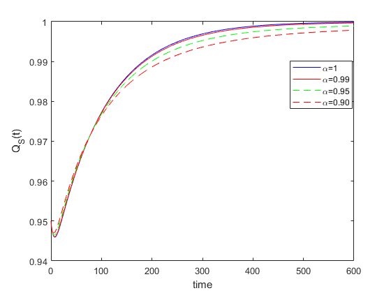
Figure 1: Solution trajectories for susceptible individuals illustrating asymptotic stability of the disease-free equilibrium $H_{df}$ with fractional orders $\alpha\in\{1,\ 0.99,\ 0.95,\ 0.90\}$ and $R_{0}<1.$

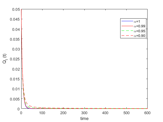
Figure 2: Solution trajectories for infected individuals illustrating asymptotic stability of the disease-free equilibrium $H_{df}$ with fractional orders $\alpha\in\{1,\ 0.99,\ 0.95,\ 0.90\}$ and $R_{0}<1.$

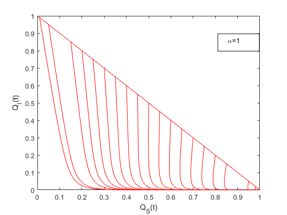
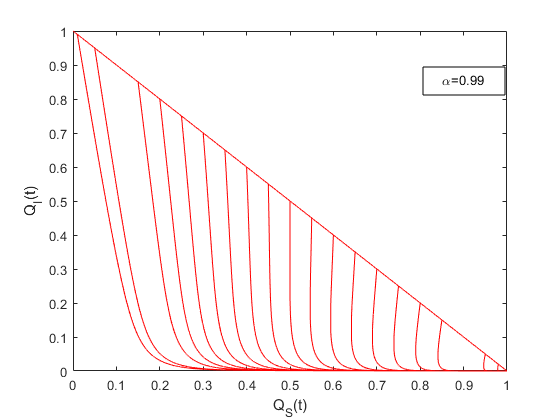
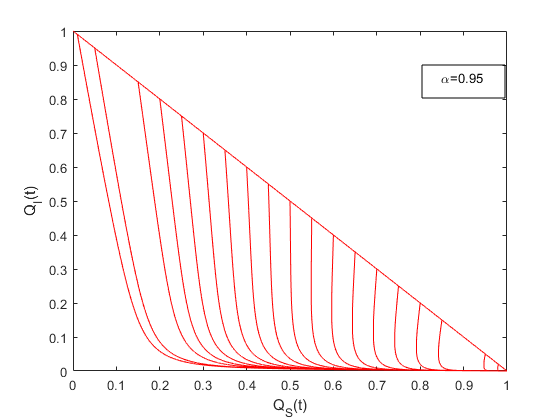
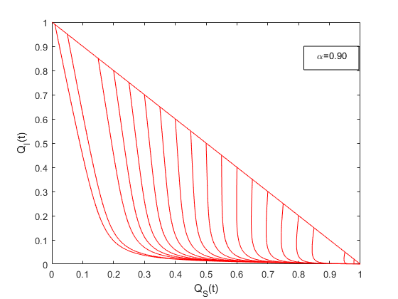
Figure 3: These graphs represent SI plane phase portraits for the SIS model with fractional orders $\alpha\in\{1,\ 0.99,\ 0.95,\ 0.90\}$ and $R_{0}<1.$

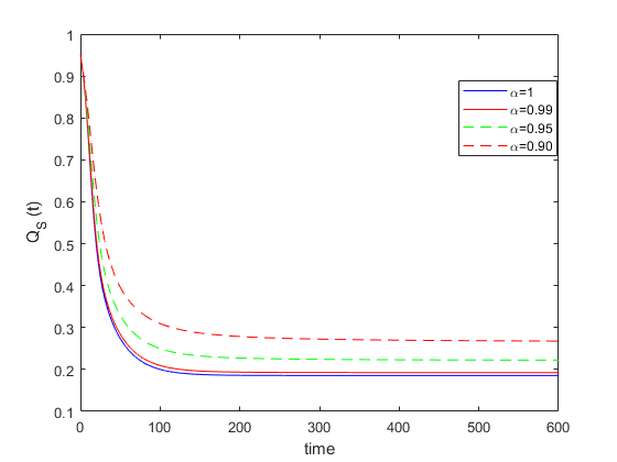
Figure 4: Solution trajectories for susceptible individuals illustrating asymptotic stability of the endemic equilibrium $H_{en}$ with fractional orders $\alpha\in\{1,\ 0.99,\ 0.95,\ 0.90\}$ and $R_{0}>1.$

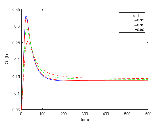
Figure 5: Solution trajectories for infected individuals illustrating asymptotic stability of the disease-free equilibrium $H_{en}$ with fractional orders $\alpha\in\{1,\ 0.99,\ 0.95,\ 0.90\}$ and $R_{0}>1.$

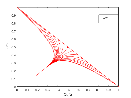
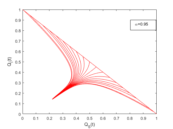
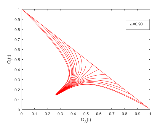
Figure 6: These graphs represent SI plane Phase portraits for the SIS model with fractional orders $\alpha\in\{1,\ 0.99,\ 0.95,\ 0.90\}$ and $R_{0}>1.$

4 SIRS model with fractional order dynamics

In this section, we introduce a new SIRS model that is characterised by system of nonlinear fractional order equations with standard incidence rate. This type of compartmental structure (susceptible-infected-recovered-susceptible) is used to construct and formulate nonlinear dynamical models for infectious diseases that that do not confer permanent immunity. The total population is grouped into three sub-populations namely susceptible individuals, $Q_{S}$, infected individuals, $Q_{I}$ and recovered individuals, $Q_{R}$. The integer order SIRS model studied in (Vargas-De-Leó, 2011, Mena-Lorca and Hethcote, 1992) is given by

$$\frac{dQ_{S}(t)}{dt} =\Lambda-\dfrac{\varphi Q_{S}Q_{I}}{Q_{S}+Q_{I}+Q_{R}}-\nu Q_{S}+\gamma Q_{R}$$

$$\frac{dQ_{I}(t)}{dt} =\dfrac{\varphi Q_{S}Q_{I}}{Q_{S}+Q_{I}+Q_{R}}-\big{(}\delta+\kappa+\nu\big{)}Q_{I}$$

$$\frac{dQ_{R}(t)}{dt} =\kappa Q_{I}-(\nu+\gamma)Q_{R}$$

where the positive model parameters which include $\Lambda,\ \varphi,\ \nu,\ \delta,\ \kappa$ and $\gamma$ represent recruitment rate, infection rate, natural death rate, recovered rate, disease induced death rate, and the loss of immunity rate respectively.

Motivated by the deterministic model (4), analyzed by the authors (Vargas-De-Leó, 2011, Mena-Lorca and Hethcote, 1992) and the fractional order modeling approach proposed in (Diethelm, 2013), the new fractional order dynamical system we consider in this study is given by

$$D_{t}^{\alpha}Q_{S}(t) =\Lambda^{\alpha}-\dfrac{\varphi^{\alpha}Q_{S}Q_{I}}{Q_{S}+Q_{I}+Q_{R}}-\nu^{\alpha}Q_{S}+\gamma^{\alpha}Q_{R}$$

$$D_{t}^{\alpha}Q_{I}(t) =\dfrac{\varphi^{\alpha}Q_{S}Q_{I}}{Q_{S}+Q_{I}+Q_{R}}-\big{(}\delta^{\alpha}+\kappa^{\alpha}+\nu^{\alpha}\big{)}Q_{I}$$

$$D_{t}^{\alpha}Q_{R}(t) =\kappa^{\alpha}Q_{I}-(\nu^{\alpha}+\gamma^{\alpha})Q_{R}$$

Knowing that $N=Q_{S}+Q_{I}+Q_{R}$, the fractional order equation describing the dynamics of the total population is given by

$$D_{t}^{\alpha}N =\Lambda^{\alpha}-\delta^{\alpha}Q_{I}-\nu^{\alpha}N$$ (10)

Since the right-hand side of equation (10) is not equal to zero, it follows that the total population may vary in time.

4.1 Equilibrium Points and local stability analysis

The disease-free and endemic equilibrium points resulting from equating the right-hand side of the dynamical system (4) to zero and solving for the states variables $Q_{S},\ \ Q_{I}$ and $Q_{R}$ yields $P_{df}=\bigg{(}\frac{\Lambda^{\alpha}}{\nu^{\alpha}},0,0\bigg{)}$ and $P_{en}=\big{(}{Q_{S}}^{*},{Q_{I}}^{*},{Q_{R}}^{*}\big{)}$ respectively, where

$${Q_{S}}^{*} =\dfrac{\Lambda^{\alpha}\big{(}\gamma^{\alpha}+\kappa^{\alpha}+\nu^{\alpha}\big{)}}{\delta^{\alpha}\big{(}\gamma^{\alpha}+\nu^{\alpha}\big{)}\big{(}R_{0}-1\big{)}+\nu^{\alpha}\big{(}\gamma^{\alpha}+\kappa^{\alpha}+\nu^{\alpha}\big{)}R_{0}}$$

$${Q_{I}}^{*} =\dfrac{\Lambda^{\alpha}\big{(}\gamma^{\alpha}+\nu^{\alpha}\big{)}\big{(}R_{0}-1\big{)}}{\delta^{\alpha}\big{(}\gamma^{\alpha}+\nu^{\alpha}\big{)}\big{(}R_{0}-1\big{)}+\nu^{\alpha}\big{(}\gamma^{\alpha}+\kappa^{\alpha}+\nu^{\alpha}\big{)}R_{0}}$$

$${Q_{R}}^{*} =\dfrac{\Lambda^{\alpha}\kappa^{\alpha}\big{(}R_{0}-1\big{)}}{\delta^{\alpha}\big{(}\gamma^{\alpha}+\nu^{\alpha}\big{)}\big{(}R_{0}-1\big{)}+\nu^{\alpha}\big{(}\gamma^{\alpha}+\kappa^{\alpha}+\nu^{\alpha}\big{)}R_{0}}$$

The basic reproduction number $R_{0}$, corresponding to the fractional dynamical model (4) is given by

$$R_{0}=\dfrac{\varphi^{\alpha}}{\big{(}\delta^{\alpha}+\kappa^{\alpha}+\nu^{\alpha}\big{)}}$$

Theorem 3

The equilibrium point $P_{df}$ (disease-free) of the SIRS model (4) is locally asymptotically stable if $R_{0}<1$ and unstable if $R_{0}>1.$

Proof. The Jacobian matrix for the dynamical fractional SIRS model computed at the equilibrium, $P_{df}$ is given by

$$J(P_{df})=\begin{bmatrix}-\nu^{\alpha}&&-\varphi^{\alpha}&&\gamma^{\alpha}\\ \\ 0&&\varphi^{\alpha}-\big{(}\delta^{\alpha}+\kappa^{\alpha}+\nu^{\alpha}\big{)}&&0\\ \\ \\ 0&&\kappa^{\alpha}&&-\big{(}\nu^{\alpha}+\gamma^{\alpha}\big{)}\end{bmatrix}$$

For the point $P_{df}$ to be locally asymptotically stable, it is necessary and sufficient to show that the all the eigenvalues of matrix $J(H_{df})$ satisfy the stability condition (6) constructed and studied in (Ahmed et al., 2006).

From the $3\times 3$ Jacobian matrix, $J(P_{df})$, it is clear that one of the eigenvalues has negative real part ($\lambda_{1}=-\nu^{\alpha}<0$) and the remaining two eigenvalues can obtained from the $2\times 2$ sub-matrix $E$ given below

$$E=\begin{bmatrix}\varphi^{\alpha}-\big{(}\delta^{\alpha}+\kappa^{\alpha}+\nu^{\alpha}\big{)}&&0\\ \\ \\ \kappa^{\alpha}&&-\big{(}\nu^{\alpha}+\gamma^{\alpha}\big{)}\end{bmatrix}$$

The remaining eigenvalues will also the satisfy the stability condition (6), provided the Routh-Hurwitz stability conditions for the characteristic equation of matrix $E$ are satisfied.

The characteristic equation of the $2\times 2$ sub-matrix $E$ is given by

$$\lambda^{2}+a_{1}\lambda+a_{2}=0$$ (11)

where

$$a_{1} =-\big{[}\varphi^{\alpha}-\big{(}\delta^{\alpha}+\kappa^{\alpha}+\nu^{\alpha}\big{)}\big{]}+\nu^{\alpha}+\gamma^{\alpha}$$

$$=-\big{(}\delta^{\alpha}+\kappa^{\alpha}+\nu^{\alpha}\big{)}\bigg{[}\dfrac{\varphi^{\alpha}}{\delta^{\alpha}+\kappa^{\alpha}+\nu^{\alpha}}-1\bigg{]}+\nu^{\alpha}+\gamma^{\alpha}$$

$$=\big{(}\delta^{\alpha}+\kappa^{\alpha}+\nu^{\alpha}\big{)}\bigg{[}1-\dfrac{\varphi^{\alpha}}{\delta^{\alpha}+\kappa^{\alpha}+\nu^{\alpha}}\bigg{]}+\nu^{\alpha}+\gamma^{\alpha}$$

$$=\big{(}\delta^{\alpha}+\kappa^{\alpha}+\nu^{\alpha}\big{)}\big{[}1-R_{0}\big{]}+\nu^{\alpha}+\gamma^{\alpha}>0\hskip 8.5359ptif\hskip 8.5359ptR_{0}<1$$

$$a_{2} =\big{(}-\nu^{\alpha}-\gamma^{\alpha}\big{)}\big{[}\varphi^{\alpha}-\big{(}\delta^{\alpha}+\kappa^{\alpha}+\nu^{\alpha}\big{)}\big{]}$$

$$=-\big{(}\nu^{\alpha}+\gamma^{\alpha}\big{)}\big{(}\delta^{\alpha}+\kappa^{\alpha}+\nu^{\alpha}\big{)}\bigg{[}\dfrac{\varphi^{\alpha}}{\delta^{\alpha}+\kappa^{\alpha}+\nu^{\alpha}}-1\bigg{]}$$

$$=\big{(}\nu^{\alpha}+\gamma^{\alpha}\big{)}\big{(}\delta^{\alpha}+\kappa^{\alpha}+\nu^{\alpha}\big{)}\big{[}1-R_{0}\big{]}>0\hskip 8.5359ptif\hskip 8.5359ptR_{0}<1$$

Since the Routh-Hurwitz stability conditions ($a_{1}>0,\ a_{2}>0,$) have been verified, it follows that the two eigenvalues will have negative real parts.   

We now consider local stability of the equilibrium point $P_{en}$. The Jacobian matrix of the fractional order model (4) evaluated at $P_{en}$ is given as follows

$$J(P_{en})=\begin{bmatrix}-\nu^{\alpha}-\frac{\varphi^{\alpha}{Q_{I}}^{*}\big{(}{Q_{I}}^{*}+{Q_{R}}^{*}\big{)}}{\big{(}{Q_{S}}^{*}+{Q_{I}}^{*}+{Q_{R}}^{*}\big{)}^{2}}&&-\frac{\varphi^{\alpha}{Q_{S}}^{*}\big{(}{Q_{S}}^{*}+{Q_{R}}^{*}\big{)}}{\big{(}{Q_{S}}^{*}+{Q_{S}}^{*}+{Q_{R}}^{*}\big{)}^{2}}&&\gamma^{\alpha}+\frac{\varphi^{\alpha}{Q_{S}}^{*}{Q_{I}}^{*}}{\big{(}{Q_{S}}^{*}+{Q_{I}}^{*}+{Q_{R}}^{*}\big{)}^{2}}\\ \\ \\ \frac{\varphi^{\alpha}{Q_{I}}^{*}\big{(}{Q_{I}}^{*}+{Q_{R}}^{*}\big{)}}{\big{(}{Q_{S}}^{*}+{Q_{I}}^{*}+{Q_{R}}^{*}\big{)}^{2}}&&\frac{\varphi^{\alpha}{Q_{S}}^{*}\big{(}{Q_{S}}^{*}+{Q_{R}}^{*}\big{)}}{\big{(}{Q_{S}}^{*}+{Q_{I}}^{*}+{Q_{R}}^{*}\big{)}}-\big{(}\delta^{\alpha}+\kappa^{\alpha}+\nu^{\alpha}\big{)}&&-\frac{\varphi^{\alpha}{Q_{S}}^{*}{Q_{I}}^{*}}{\big{(}{Q_{S}}^{*}+{Q_{I}}^{*}+{Q_{R}}^{*}\big{)}^{2}}\\ \\ \\ 0&&\kappa^{\alpha}&&-\big{(}\nu^{\alpha}+\gamma^{\alpha}\big{)}\end{bmatrix}$$

Using the identity $\dfrac{\varphi^{\alpha}{Q_{S}}^{*}}{{Q_{S}}^{*}+{Q_{I}}^{*}+{Q_{R}}^{*}}=\big{(}\delta^{\alpha}+\kappa^{\alpha}+\nu^{\alpha}\big{)}$, the Jacobian matrix can be simplified as

$$J(P_{en})=\begin{bmatrix}-\nu^{\alpha}-\frac{\varphi^{\alpha}{Q_{I}}^{*}\big{(}{Q_{I}}^{*}+{Q_{R}}^{*}\big{)}}{\big{(}{Q_{S}}^{*}+{Q_{I}}^{*}+{Q_{R}}^{*}\big{)}^{2}}&&-\frac{\varphi^{\alpha}{Q_{S}}^{*}\big{(}{Q_{S}}^{*}+{Q_{R}}^{*}\big{)}}{\big{(}{Q_{S}}^{*}+{Q_{I}}^{*}+{Q_{R}}^{*}\big{)}^{2}}&&\gamma^{\alpha}+\frac{\varphi^{\alpha}{Q_{S}}^{*}{Q_{I}}^{*}}{\big{(}{Q_{S}}^{*}+{Q_{I}}^{*}+{Q_{R}}^{*}\big{)}^{2}}\\ \\ \frac{\varphi^{\alpha}{Q_{I}}^{*}\big{(}{Q_{I}}^{*}+{Q_{R}}^{*}\big{)}}{\big{(}{Q_{S}}^{*}+{Q_{I}}^{*}+{Q_{R}}^{*}\big{)}^{2}}&&-\frac{\varphi^{\alpha}{Q_{S}}^{*}{Q_{I}}^{*}}{\big{(}{Q_{S}}^{*}+{Q_{I}}^{*}+{Q_{R}}^{*}\big{)}^{2}}&&-\frac{\varphi^{\alpha}{Q_{S}}^{*}{Q_{I}}^{*}}{\big{(}{Q_{S}}^{*}+{Q_{I}}^{*}+{Q_{R}}^{*}\big{)}^{2}}\\ \\ 0&&\kappa^{\alpha}&&-\big{(}\nu^{\alpha}+\gamma^{\alpha}\big{)}\end{bmatrix}$$

The characteristic equation of matrix $J(P_{en})$ is given as follows

$$\lambda^{3}+w_{1}\lambda^{2}+w_{2}\lambda+w_{3}=0,$$ (12)

where

$$w_{1} =\frac{\varphi^{\alpha}{Q_{I}}^{*}\big{(}{Q_{I}}^{*}+{Q_{R}}^{*}\big{)}}{\big{(}{Q_{S}}^{*}+{Q_{I}}^{*}+{Q_{R}}^{*}\big{)}^{2}}+\frac{\varphi^{\alpha}{Q_{S}}^{*}{Q_{I}}^{*}}{\big{(}{Q_{S}}^{*}+{Q_{I}}^{*}+{Q_{R}}^{*}\big{)}^{2}}+2\nu^{\alpha}+\gamma^{\alpha}$$

$$w_{2} =\dfrac{(\varphi^{\alpha})^{2}{Q_{I}}^{*}{Q_{S}}^{*}\big{(}{Q_{I}}^{*}+{Q_{R}}^{*}\big{)}\big{(}{Q_{S}}^{*}+{Q_{R}}^{*}\big{)}}{\big{(}{Q_{S}}^{*}+{Q_{I}}^{*}+{Q_{R}}^{*}\big{)}^{4}}+\frac{(\varphi^{\alpha})^{2}{Q_{S}}^{*}({Q_{I}}^{*})^{2}\big{(}{Q_{I}}^{*}+{Q_{R}}^{*}\big{)}}{\big{(}{Q_{S}}^{*}+{Q_{I}}^{*}+{Q_{R}}^{*}\big{)}^{4}}$$

$$+\frac{\kappa^{\alpha}\varphi^{\alpha}{Q_{S}}^{*}{Q_{I}}^{*}}{\big{(}{Q_{S}}^{*}+{Q_{I}}^{*}+{Q_{R}}^{*}\big{)}^{2}}+\frac{\nu^{\alpha}\varphi^{\alpha}{Q_{I}}^{*}\big{(}{Q_{I}}^{*}+{Q_{R}}^{*}\big{)}}{\big{(}{Q_{S}}^{*}+{Q_{I}}^{*}+{Q_{R}}^{*}\big{)}^{2}}+\frac{2\nu^{\alpha}\varphi^{\alpha}{Q_{S}}^{*}{Q_{I}}^{*}}{\big{(}{Q_{S}}^{*}+{Q_{I}}^{*}+{Q_{R}}^{*}\big{)}^{2}}$$

$$+\frac{\gamma^{\alpha}\varphi^{\alpha}{Q_{I}}^{*}\big{(}{Q_{I}}^{*}+{Q_{R}}^{*}\big{)}}{\big{(}{Q_{S}}^{*}+{Q_{I}}^{*}+{Q_{R}}^{*}\big{)}^{2}}+\frac{\gamma^{\alpha}\varphi^{\alpha}{Q_{S}}^{*}{Q_{I}}^{*}}{\big{(}{Q_{S}}^{*}+{Q_{I}}^{*}+{Q_{R}}^{*}\big{)}^{2}}+\nu^{\alpha}\gamma^{\alpha}+(\nu^{\alpha})^{2}$$

$$w_{3} =\frac{\nu^{\alpha}(\varphi^{\alpha})^{2}{Q_{S}}^{*}{Q_{I}}^{*}\big{(}{Q_{I}}^{*}+{Q_{R}}^{*}\big{)}\big{(}{Q_{S}}^{*}+{Q_{R}}^{*}\big{)}}{\big{(}{Q_{S}}^{*}+{Q_{I}}^{*}+{Q_{R}}^{*}\big{)}^{4}}+\frac{\nu^{\alpha}(\varphi^{\alpha})^{2}({Q_{I}}^{*})^{2}{Q_{S}}^{*}\big{(}{Q_{I}}^{*}+{Q_{R}}^{*}\big{)}}{\big{(}{Q_{S}}^{*}+{Q_{I}}^{*}+{Q_{R}}^{*}\big{)}^{4}}$$

$$+\frac{\gamma^{\alpha}(\varphi^{\alpha})^{2}{Q_{S}}^{*}{Q_{I}}^{*}\big{(}{Q_{I}}^{*}+{Q_{R}}^{*}\big{)}\big{(}{Q_{S}}^{*}+{Q_{R}}^{*}\big{)}}{\big{(}{Q_{S}}^{*}+{Q_{I}}^{*}+{Q_{R}}^{*}\big{)}^{4}}+\frac{\gamma^{\alpha}(\varphi^{\alpha})^{2}({Q_{I}}^{*})^{2}{Q_{S}}^{*}\big{(}{Q_{I}}^{*}+{Q_{R}}^{*}\big{)}}{\big{(}{Q_{S}}^{*}+{Q_{I}}^{*}+{Q_{R}}^{*}\big{)}^{4}}$$

$$+\frac{\kappa^{\alpha}\nu^{\alpha}\varphi^{\alpha}{Q_{S}}^{*}{Q_{I}}^{*}}{\big{(}{Q_{S}}^{*}+{Q_{I}}^{*}+{Q_{R}}^{*}\big{)}^{2}}+\frac{\gamma^{\alpha}\nu^{\alpha}\varphi^{\alpha}{Q_{S}}^{*}{Q_{I}}^{*}}{\big{(}{Q_{S}}^{*}+{Q_{I}}^{*}+{Q_{R}}^{*}\big{)}^{2}}-\frac{\kappa^{\alpha}\gamma^{\alpha}\varphi^{\alpha}{Q_{I}}^{*}\big{(}{Q_{I}}^{*}+{Q_{R}}^{*}\big{)}}{\big{(}{Q_{S}}^{*}+{Q_{I}}^{*}+{Q_{R}}^{*}\big{)}^{2}}$$

$$+\frac{(\nu^{\alpha})^{2}\varphi^{\alpha}{Q_{S}}^{*}{Q_{I}}^{*}}{\big{(}{Q_{S}}^{*}+{Q_{I}}^{*}+{Q_{R}}^{*}\big{)}^{2}}$$

Let $D(q)$ represent the discriminant of a polynomial function $q$ given by

$$q(x)=x^{3}+w_{1}x^{2}+w_{2}x+w_{3}$$

then

$$D(q)=\begin{vmatrix}1&w_{1}&w_{2}&w_{3}&0\\ 0&1&w_{1}&w_{2}&w_{3}\\ 3&2w_{1}&w_{2}&0&0\\ 0&3&2w_{1}&w_{2}&0\\ 0&0&3&2w_{1}&w_{2}\end{vmatrix}=18w_{1}w_{2}w_{3}+(w_{1}w_{2})^{2}-4w_{3}w_{1}^{2}-4w_{2}^{2}-27w_{3}^{2}.$$ (13)

Motivated by the fractional order stability approach in (Ahmed et al., 2006) and the recent applications of this concept in (Silva and Torres, 2019, Hamdan and Kilicman, 2018, Salman and Yousefl, 2017, Carvalho and Pinto, 2016), we obtain the proposition below

Proposition 1

One assume that $P_{en}$ exists in $\mathbb{R}^{3}_{+}.$

1. If $D(q)>0$ and the Routh-Hurwitz condition are satisfied, i.e., $w_{1}>0$, $w_{3}>0$, $w_{1}$ $w_{2}>w_{3}$, then $P_{en}$ is locally asymptotically stable.

2. If $D(q)<0$, $w_{1}\geq 0$, $w_{2}\geq 0$, $w_{3}>0$, $\alpha<2/3$ then $P_{en}$ is locally asymptotically stable.

3. If $D(q)<0$, $w_{1}<0$, $w_{2}<0$, $\alpha>2/3$ then all roots of $q(\lambda)=0$ satisfy the stability condition $\mathinner{\!\left\lvert arg(\lambda)\right\rvert}>\frac{\alpha\pi}{2}$.

4. If $D(q)<0$, $w_{1}>0$, $w_{2}>0$, $w_{1}w_{2}=w_{3}$ $\forall\alpha\in(0,1]$ then $P_{en}$ is locally asymptotically stable.

5. $w_{3}>0$ is a necessary condition for $P_{en}$ to be locally asymptotically stable.

4.2 Numerical simulations and discussions

This subsection deals with numerical approximation of the new SIRS fractional epidemic model (4). For our numerical illustrations, we have applied the fracPECE iterative scheme developed by Diethelm and Freed (1999). We have also used the Matlab code fde12.m designed by Garrappa (2011) for the fracPECE iterative scheme.

To demonstrate local asymptotic stability of the disease-free point, we considered the parameter values: $\Lambda=0.01,\ \beta=0.06,\ \nu=0.01,\ \delta=0.15,\ \kappa=0.3,\ \gamma=0.02$ and initial conditions $Q_{S0}=0.95,\ Q_{I0}=0.05,\ Q_{R0}=0$. Local asymptotic stability of the endemic point is illustrated by setting $\Lambda=0.01,\ \beta=0.5,\ \nu=0.01,\ \delta=0.015,\ \kappa=0.2,\ \gamma=0.02$ and initial conditions $Q_{S0}=0.95,\ Q_{I0}=0.05,\ Q_{R0}=0$. Figures 7, 8 and 9 shows trajectories of susceptible, infected and recovered individuals respectively for different values of $\alpha$ illustrating asymptotic stability of the disease-free equilibrium. Local asymptotic stability of the endemic equilibrium is demonstrated in Figures 11, 12 and 13. The sub-plots in Figures 10 and 14 illustrate SI plane phase portraits for the SIRS model.

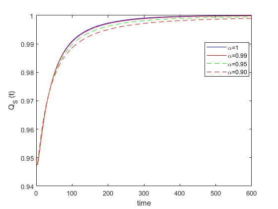
Figure 7: Solution trajectories for susceptible individuals illustrating asymptotic stability of the disease-free equilibrium $H_{df}$ with fractional orders $\alpha\in\{1,\ 0.99,\ 0.95,\ 0.90\}$ and $R_{0}<1.$

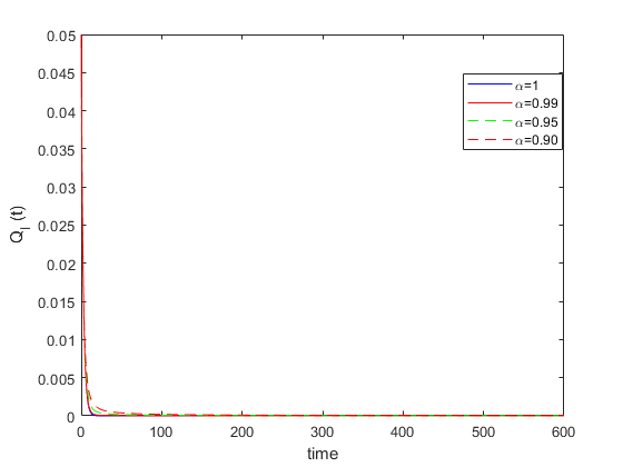
Figure 8: Solution trajectories for infected individuals illustrating asymptotic stability of the disease-free equilibrium $H_{df}$ with fractional orders $\alpha\in\{1,\ 0.99,\ 0.95,\ 0.90\}$ and $R_{0}<1.$

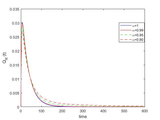
Figure 9: Solution trajectories for recovered individuals illustrating asymptotic stability of the disease-free equilibrium $H_{df}$ with fractional orders $\alpha\in\{1,\ 0.99,\ 0.95,\ 0.90\}$ and $R_{0}<1.$

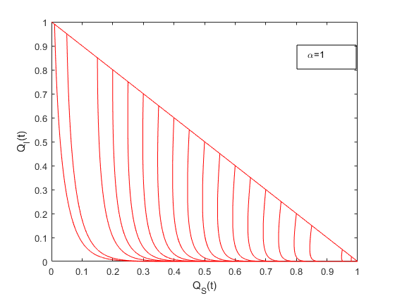
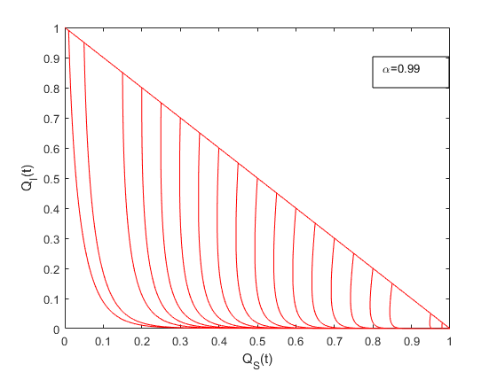
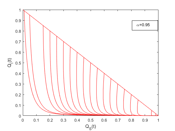
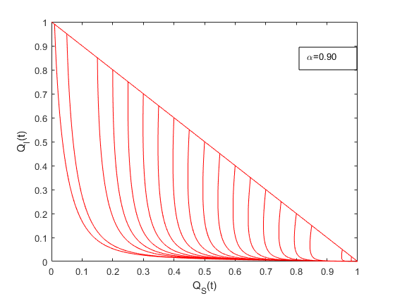
Figure 10: These sub-plots represent SI plane Phase portraits for the SIRS model with fractional orders $\alpha\in\{1,\ 0.99,\ 0.95,\ 0.90\}$ and $R_{0}<1.$

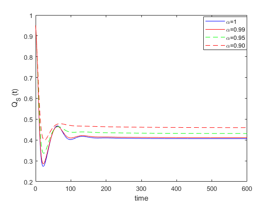
Figure 11: Solution trajectories for susceptible individuals illustrating asymptotic stability of the endemic equilibrium $P_{en}$ with fractional orders $\alpha\in\{1,\ 0.99,\ 0.95,\ 0.90\}$ and $R_{0}>1.$

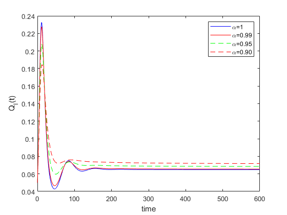
Figure 12: Solution trajectories for infected individuals illustrating asymptotic stability of the endemic equilibrium $P_{en}$ with fractional orders $\alpha\in\{1,\ 0.99,\ 0.95,\ 0.90\}$ and $R_{0}>1.$

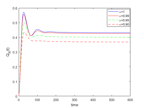
Figure 13: Solution trajectories for recovered individuals illustrating asymptotic stability of the endemic equilibrium $P_{en}$ with fractional orders $\alpha\in\{1,\ 0.99,\ 0.95,\ 0.90\}$ and $R_{0}>1.$

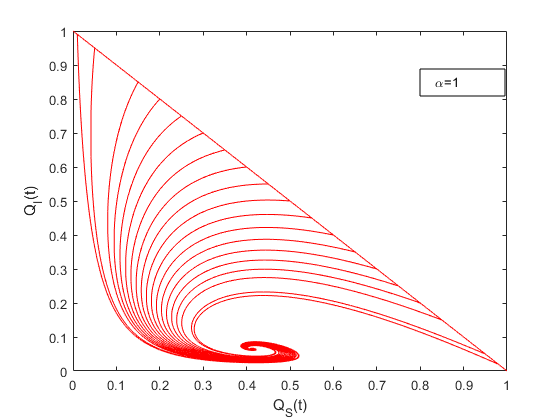
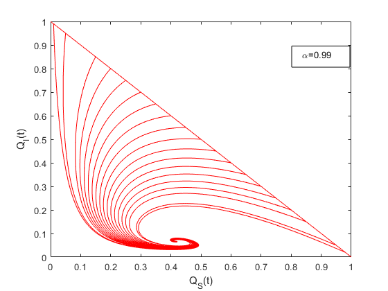
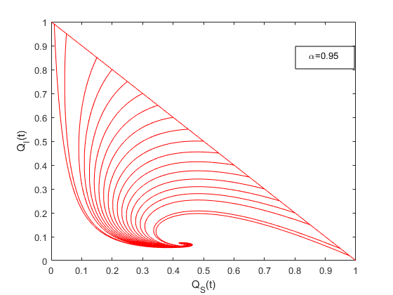
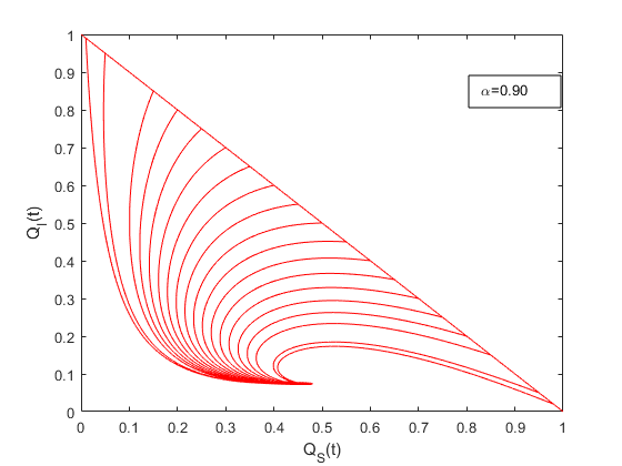
Figure 14: These sub-plots represent SI plane phase portraits for the SIRS model with fractional orders $\alpha\in\{1,\ 0.99,\ 0.95,\ 0.90\}$ and $R_{0}>1.$

5 Conclusion

In this work, we have presented and analyzed two epidemic models that are constructed with Caputo fractional derivative. Our fractional order modelling construction was motivated by the approach introduced by the author in (Diethelm, 2013). We have studied a modified fractional order SIS model from an existing mathematical model. A new Caputo based SIRS model is also proposed and analyzed. In both mathematical models, we have analytically and numerically studied local asymptotic stability of the equilibrium points (disease-free and endemic). Our numerical examples suggest that, fractional order models are appropriate for compartmental modeling of infectious diseases dynamics and can yield interesting results.

References

• Ahmed and El-Saka (2010) E. Ahmed and H. A. El-Saka. On fractional order models for hepatitis c. Nonlinear Biomedical Physics., 4:1–3, 2010.
• Ahmed et al. (2006) E. Ahmed, A. M. A. El-Sayed, and H. A. A. El-Saka. On some routh–hurwitz conditions for fractional order differential equations and their applications in Lorenz, Rössler, Chua and Chen systems. Physics Letters A, 358:1–4, 2006.
• Almeida (2018) R. Almeida. Analysis of a fractional SEIR model with treatment. Applied Mathematics Letters, 84:56–62, 2018.
• Almeida et al. (2019) Ricardo Almeida, Artur MC Brito da Cruz, Natália Martins, and M Teresa T Monteiro. An epidemiological MSEIR model described by the caputo fractional. Intentional Journal of Dynamics and Control, 7(2):776–784, 2019.
• Ameen and Novati (2017) I. Ameen and P. Novati. The solution of fractional order epidemic model by implicit Adams methods. Applied Mathematical Modelling, 43:78–84, 2017.
• Arafa et al. (2012) A. A. M. Arafa, S. Z. Rida, and M. Khalil. Solution of fractional order model of childhood diseases with constant vaccination strategy. Mathematical Sciences Letters, 1:17–23, 2012.
• Boukhouima et al. (2018) A. Boukhouima, K. Hattaf, and N. Yousfi. A fractional order model for viral infection with cure of infected cells and humoral immunity. International Journal of Differential Equations, 2018, Article ID 101242:12, 2018.
• Carvalho and Pinto (2016) A. Carvalho and C. M. A. Pinto. A delay fractional order model for the co-infection of malaria and HIV/ AIDS. International Journal of Dynamics and Control, 5:168, 2016.
• Carvalho et al. (2018) A. R. M. Carvalho, C. M. A. Pinto, and D. Baleanu. HIV/HCV coinfection model: a fractional-order perspective for the effect of the HIV viral load. Advances in Difference Equations, page 2, 2018. doi: 10.1186/s13662-017-1456-z. URL https://doi.org/10.1186/s13662-017-1456-z.
• Diethelm (2013) K. Diethelm. A fractional calculus based model for the simulation of an outbreak of dengue fever. Nonlinear Dynamics, 71:613–619, 2013.
• Diethelm and Freed (1999) K. Diethelm and A.D. Freed. TheFrac PECE subroutine for the numerical solution of differential equations of fractional order, in: S. Heinzel, T. Plesser (Eds.), Forschung und Wissenschaftliches Rechnen 1998, Gessellschaft fur Wissenschaftliche Datenverarbeitung, Gottingen. pages 57–71, 1999.
• El-Saka (2013) H. A. A. El-Saka. The fractional-order SIR and SIRS epidemic models with variable population size. Mathematical Sciences Letters, 2(3):195, 2013.
• El-Saka (2014) H. A. A. El-Saka. The fractional-order SIS epidemic model with variable population. Journal of the Egyptian Mathematical Society, 22(1):50–54, 2014.
• El-Saka et al. (2019) H. A. A. El-Saka, A. A. M. Arafa, and M. I Gouda. Dynamical analysis of a fractional SIRS model on homogenous networks. Advances in Difference Equations, 2019(1):144, 2019.
• Garrappa (2011) R. Garrappa. Predictor-corrector PECE method for fractional differential equations, MATLAB Central File Exchange. File ID: 32918, 2011.
• González-Parra et al. (2014) G. González-Parra, A. J. Arenas, and B. Chen-Charpentier. A fractional order epidemic model for the simulation of outbreaks of influenza A(H1N1). Mathematical Methods in the Applied Sciences, 37:2218–2226, 2014.
• Hamdan and Kilicman (2018) N. I. Hamdan and A. Kilicman. A fractional order SIR epidemic model for dengue transmission. Chaos, Solitons & Fractals, 114:55–62, 2018.
• Hassouna et al. (2018) M. Hassouna, A. Ouhadan, and E. H. El. Kinani. On the solution of fractional order SIS epidemic. Chaos, Solitons & Fractals, 117:168–174, 2018.
• Hethcote (2000) H. W. Hethcote. The mathematics of infectious diseases. Siam Review, 42:599–653, 2000.
• Jajarmi et al. (2019) A. Jajarmi, S. Arshad, and D. Baleanu. A new fractional modelling and control strategy for the outbreak of dengue fever. Physica A: Statistical Mechanics and its Applications, 535:122524, 2019.
• Liu et al. (2019) N. Liu, J. Fang, W. Deng, and J-W. Sun. Stability analysis of a fractional-order SIS model on complex networks with linear treatment function. Advances in Difference Equations, 2019(1):1–10, 2019.
• Mena-Lorca and Hethcote (1992) J. Mena-Lorca and H. W. Hethcote. Dynamic models of infectious diseases as regulators of population sizes. Journal of Mathematical Biology, 30(7):693–716, 1992.
• Mouaouine et al. (2018) A. Mouaouine, A. Boukhouima, K. Hattaf, and N. Yousfi. A fractional order SIR epidemic model with nonlinear incidence rate. Advances in Difference Equations, 2018(1):160, 2018.
• Okyere et al. (2016) E. Okyere, F. T. Oduro, S. K. Amponsah, I. K. Dontwi, and N. K. Frempong. Fractional order SIR model with constant population. British Journal of Mathematics and Computer Science, 14:1–12, 2016.
• Ozalp and Demirci (2011) N. Ozalp and E. Demirci. A fractional order SEIR model with vertical transmission. Mathematical and Computer Modelling, 54:1–6, 2011.
• Petras (2011) I. Petras. Fractional-Order Nonlinear Systems: Modeling, Analysis and Simulation. Springer, 2011.
• Pinto and Carvalho (2019) C. M. A. Pinto and A. R. M. Carvalho. Diabetes mellitus and TB co-existence: Clinical implications from a fractional order modelling. Applied Mathematical Modelling, 68:219–243, 2019.
• Podlubny (1999) I. Podlubny. Fractional Differential Equations. Academic Press, New York, 1999.
• Qureshi and Atangana (2019) S. Qureshi and A. Atangana. Mathematical analysis of dengue fever outbreak by novel fractional operators with field data. Physica A, 526:121127, 2019.
• Qureshi and Yusuf (2019) Sania Qureshi and Abdullahi Yusuf. Fractional derivatives applied to MSEIR problems: Comparative study with real world data. The European Physical Journal Plus, 134(4):171, 2019.
• R. Jan et al. (2019) Rashid R. Jan, M. A. Khan, P. Kumam, and P. Thounthong. Modeling the transmission of dengue infection through fractional derivatives. Chaos, Solitons & Fractals, 127:189–216, 2019.
• Rihan et al. (2019) F. A. Rihan, Q. M. Al-Mdallal, H. J. AlSakaji, and A. Hashish. A fractional-order epidemic model with time-delay and nonlinear incidence rate. Chaos, Solitons & Fractals, 126:97–105, 2019.
• Salman and Yousefl (2017) S. M. Salman and A. M. Yousefl. On a fractional-order model for HBV infection with cure of infected cells. Journal of Egyptian Mathematical Societys, 25:445–451, 2017.
• Sardar et al. (2015) T. Sardar, S. Rana, S. Bhattacharya, K. Al-Khaled, and J. Chattopadhyay. A generic model for a single strain mosquito-transmitted disease with memory on the host and the vector. Mathematical biosciences, 263:18–38, 2015.
• Silva and Torres (2019) C. J. Silva and D. F. M. Torres. Stability of a fractional HIV/AIDS model. Mathematics and Computers in Simulation, 164:180–190, 2019.
• Ullah et al. (2018) S. Ullah, M. A. Khan, and M. Farooq. A new fractional model for the dynamics of the hepatitis B virus using the caputo-fabrizio derivative. The European Physical Journal Plus, 133(6):237, 2018.
• Vargas-De-Leó (2011) C. Vargas-De-Leó. On the global stability of SIS, SIR and SIRS epidemic models with standard incidence. Chaos, Solitons & Fractals, 44:1106–1110, 2011.
• Vargas-De-Leó (2015) C. Vargas-De-Leó. Volterra-type lyapunov functions for fractional-order epidemic systems. Communications in Nonlinear Science and Numerical Simulation, 24(1-3):75–85, 2015.
• Wang et al. (2019) X. Wang, Z. Wang, and J. Xia. Stability and bifurcation control of a delayed fractional-order eco-epidemiological model with incommensurate orders. Journal of the Franklin Institute, 356(15):8278–8295, 2019.