Nonaxisymmetric Component of Solar Activity and the Gnevyshev-Ohl rule

1 Introduction

S-Introduction

Observations of the Sun, solar activity and its cyclic changes have a long history, although the beginning of a truly systematic collection of sunspot data should apparently be attributed to the observations of M. Schwabe and R. Wolf in the mid-19th century. Later it became clear that variations in activity are connected with changes in the magnetic fields of the Sun. To the first attempts to explain the 11-year cyclicity of these phenomena belongs the development of the Babcock–Leighton solar dynamo model (Babcock, 1961; Leighton, 1969). This model and a number of its improvements are based on the notion of axisymmetry of the solar magnetic field (see the survey Charbonneau, 2010). However, at present it is believed that the violation of axisymmetry, which manifests itself in the form of active longitudes, is not accidental, but is one of important components of the solar cycle. According to (Ruzmaikin, 2001), nonaxisymmetric mode even prevails at the time of solar maximum as compared with the axisymmetric mode. Active longitudes were called one of the most interesting manifestations of the solar nonaxisymmetric magnetic field (Pipin and Kosovichev, 2015). It was shown that active longitudes appear also on some types of the stars (Tuominen, Berdyugina and Korpi, 2002) occupying alternately diametrically opposite longitudes (flip-flop). The problem of active longitudes is treated in a large number of works, both experimental and theoretical (see, e.g., Gaizauskas, 1993; Bai, 2003; Bigazzi and Ruzmaikin, 2004; Pipin et al., 2019 and references therein).

Development of solar cycle models which include the generation of nonaxisymmetric magnetic fields should be based on reliable set of data. At present some of results obtained in different studies of active longitudes are contradictive. E.g., the lifetime of active longitudes according to different studies varies from several solar rotations (de Toma, White, and Harvey, 2000) to 20–40  rotations (Bumba and Howard, 1969) and even longer than one 11-year cycle (Balthasar and Schüssler, 1983; Bai, 1988; Jetsu et al., 1997). Around solar minimum, sunspots of the new cycle tend to concentrate at the same active longitudes as the sunspots of the previous cycle (Benevolenskaya et al., 1999; Benevolenskaya and Kostuchenko, 2013).

Results of some studies support the rigid rotation of active longitudes with the nearly Carrington period (Bumba and Howard, 1969); Gaizauskas, 1993). It was also found in some of theoretical models (Pipin and Kosovichev, 2015) that the dynamo-generated nonaxisymmetric magnetic field rotates rigidly. The speed of the solar wind and interplanetary magnetic field display a connection with the rigidly rotating active longitudes (Neugebauer et al., 2000). Other authors, analyzing the experimental data come to a conclusion that the speed of rotation of active longitudes depends on the latitude and is determined by the Sun’s differential rotation speed (Berdyugina and Usoskin, 2003). This shows that the active longitude problem is a topic of current interest and there are many open questions related to this phenomenon.

In the paper Vernova et al. (2004), the analysis of the distribution of sunspot area over the longitudes showed that active longitudes manifest themselves successively at $180^{\circ}$ during the ascend and maximum phases of the solar cycle and at $0^{\circ}/360^{\circ}$ during the phases of descend and minimum. The change of the location occurs in the period of the sign change of the leading sunspots at the minimum of the solar activity and in the period of the polar field reversal. An analogous pattern was observed for the X-ray flares of classes M and X (Vernova, Tyasto and Baranov, 2005) and photospheric magnetic fields.

The same localization of active longitudes ($180^{\circ}$ and $0^{\circ}/360^{\circ}$) was discovered in major solar flares (Dodson and Hedeman, 1968; Jetsu et al., 1997). Activity complex connected with a number of solar flares occupied longitudes around $180^{\circ}$ during solar maximum of 1991 (Bumba et al., 1996). Preferred longitudes shifting from $180^{\circ}$ to $30^{\circ}$ were found in CME (Coronal Mass Ejections) distribution (Skirgiello, 2005) with the change of the location at the time of transition from the ascend-maximum phase to the descend-minimum and vice versa.

The aim of the present work is to study the nonaxisymmetric component of the solar activity during 13 solar cycles (1874–2016). Section S-Data describes data used in this study and method of the data treatment. In Section S-Asymmetry evolution of the nonaxisymmetric component is considered. Section S-Phase is dedicated to the problem of active longitudes. In Section S-Conclusions main conclusions are drawn.

2 Data and Method

S-Data

To study the nonaxisymmetric component of the solar activity we used the vector representation of the sunspot data. The areas and heliocoordinates of sunspots for 1874–2016 were obtained at the site of Royal Observatory, Greenwich–USAF/NOAA Sunspot Data (https://solarscience.msfc.nasa.gov/greenwch.shtml). A polar vector was assigned to each of the sunspots observed during Carrington rotation, the magnitude of the vector being set equal to the sunspot area $Sp$ and the phase angle was defined as the heliolongitude of the sunspot $L$. Individual vectors were combined by vector summing into one resulting vector for each solar rotation (Vernova et al., 2002). The magnitude of the resulting vector could be interpreted as the quantitative characteristics of the nonaxisymmetric component of solar activity while the phase angle pointed to the preferred longitude. We shall refer to the resulting vector as the vector of the longitudinal asymmetry and to its modulus as the longitudinal asymmetry (LA).

The method of the data treatment is illustrated by the scheme in Figure schemea,b. Schematic drawing of the solar disk with two sunspots is shown in Figure schemea, while in Figure schemeb the corresponding polar vectors are shown. Resulting vector for the day of observation is displayed as the red arrow.

For a given day (with number $k$) we calculated the vector sum of all polar vectors ${\mathbfit S}_{i,k}$ corresponding to all $N$ sunspots observed during this day $(i=1,\dots,N)$. In Figure schemeb the vector sum for two sunspots observed during a day is shown by a red arrow. Finally, for each solar rotation we defined the resulting vector ${\mathbfit S}$ as the vector sum of daily vectors for all days of the rotation $(k=1,\dots,27)$. This procedure can be expressed by the equation

$$\ilabel{1}{\mathbfit S}=\sum_{i,k}{\mathbfit S}_{i,k}.$$ (1)

The vector summing technique allowed us to separate the nonaxisymmetric component of the longitudinal distribution of sunspots represented by the vector of the longitudinal asymmetry ${\mathbfit S}$, whose magnitude (modulus) will be referred to as the longitudinal asymmetry ($LA=|{\mathbfit S}|$). The vector phase $L$ points to the dominating longitude.

The vector of the longitudinal asymmetry has the following important features. Sunspot groups living several days or longer make corresponding number of contributions into the vector of the longitudinal asymmetry ${\mathbfit S}$. Therefore large long-living sunspot groups play the main role in the magnitude of the longitudinal asymmetry vector. Due to the vector summing the influence of the solar activity component uniformly distributed over longitude was reduced and the stable nonaxisymmetric component of the solar activity distribution was singled out.

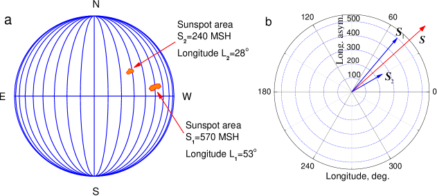
Figure 1.: Vector representation of solar activity (scheme). (a) Schematic drawing of the Sun with two sunspots on the disk with areas $S_{1}$, $S_{2}$. (b) Polar diagram showing two polar vectors assigned to the sunspots 1 and 2. The moduli of these vectors are set equal to the sunspot areas, the phases are defined as the longitude of sunspots. The red arrow corresponds to the vector sum of the individual vectors. scheme

Due to the vector summing method the influence of the stochastic component of the solar activity uniformly distributed over longitude was reduced and the stable nonaxisymmetric component of the solar activity distribution was singled out.

The vector of the longitudinal asymmetry was defined for an integer number of days ($T=27$ days), while a Carrington rotation period is 27.2753 days. The time shift which occurs as a result of this difference is not large but it accumulates and can affect significantly the assignment of the longitudinal asymmetry to a specific time. To compensate this time shift we used the method where for several rotations the asymmetry was calculated for the period $T=27$ days, after which for one rotation the asymmetry was calculated for the period $T=28$ days. These scheme allowed to avoid accumulation of errors and to get the time shift of at most 5 days during the whole, almost 150 year long, period under consideration.

The longitudinal asymmetry vector can be also computed for some specific groups of sunspots, e.g., for sunspots whose area is above (or below) some chosen threshold.

3 Nonaxisymmetric component of the solar activity (modulus of the vector of the longitudinal asymmetry)

S-Asymmetry

3.1 Time variation of the longitudinal asymmetry

S-Time Using the method described above we calculated the magnitude and phase angle of the vector of the longitudinal asymmetry for the whole disc of the Sun as well as separately for the northern and southern hemispheres. The modulus of the vector of the longitudinal asymmetry (to be short, the longitudinal asymmetry, or LA) can be considered as a quantitative characterstics of the nonaxisymmetric component of the solar activity.

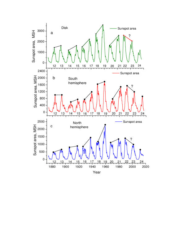
Figure 2.: Sunspot area for Solar Cycles 12–24 (1874–2016): (a) solar disk; (b) southern hemisphere; (c) northern hemisphere. Solar Cycle numbers are shown at the bottom of the panels. Maximums of the even cycles ($2N$) and the following odd cycles ($2N+1$) are connected by straight line segments to emphasize the manifestation of the Gnevyshev–Ohl rule. Curves were smoothed using 13-rotation running mean. area

We compared the variations of the longitudinal asymmetry during 13 solar cycles with the corresponding variations of the sunspot area.In Figure area changes in time (1874–2016) of the sunspot area are shown for the whole disc (Figure areaa), southern hemisphere (Figure areab) and northern hemisphere (Figure areac).

One of the repeating patterns of the solar activity variations is the Gnevyshev–Ohl rule (Gnevyshev and Ohl, 1948). There exist different formulations of this rule which manifests itself in many solar activity parameters. The Gnevyshev–Ohl rule as well as its violations are treated in numerous papers (e.g., Nagovitsyn, Nagovitsyna and Makarova, 2009, Ogurtsov, 2012, Javaraiah, 2013).

One of the forms of the Gnevyshev–Ohl (G-O) rule is as follows: the amplitude of an even solar cycle (cycle $2N$) is lower than the amplitude of the following odd cycle (cycle $2N+1$). The Gnevyshev–Ohl rule holds for ten solar cycles (Solar Cycles 12–21). This pattern is shown in Figure area; to stress the relation between the cycle heights the straight line segments are drawn connecting the maxima of an even and of the consequent odd cycles. It is seen that the G-O rule holds similarly for the disc and for the southern and the northern hemispheres. It should be noted that in the sunspot area the highest is Solar Cycle 19 and one of the lowest is Solar Cycle 20, and these features are present for the whole disc as well as for the both hemispheres.

It was shown in many studies that the G-O rule does not hold for the pair of Solar Cycles 22–23. This violation of the general rule can be seen in Figures areaa,b,c also. As an explanation of the G-O rule violation in Solar Cycles 22–23 Javaraiah (2016) points out to the contribution of small sunspot groups with area below 100 MSH (millionths of solar hemisphere). The number of such groups was large in the southern hemisphere during Solar Cycle 22, whereas in Solar Cycle 23 the number of such groups was low in both hemispheres

Time variations of the nonaxisymmetric component of the solar activity are shown in Figure lonasym for Solar Cycles 12–24 for the disc (Figure lonasyma), southern hemisphere (Figure lonasymb) and northern hemisphere (Figure lonasymc).

We use this specific order of the figures (disc, southern hemisphere, northern hemisphere) to emphasize the similarity of the dependencies for the disc and for the southern hemisphere. On the other hand, the modulus of the vector of the longitudinal asymmetry for the northern hemisphere differs considerably from the whole disc and from the southern hemisphere.

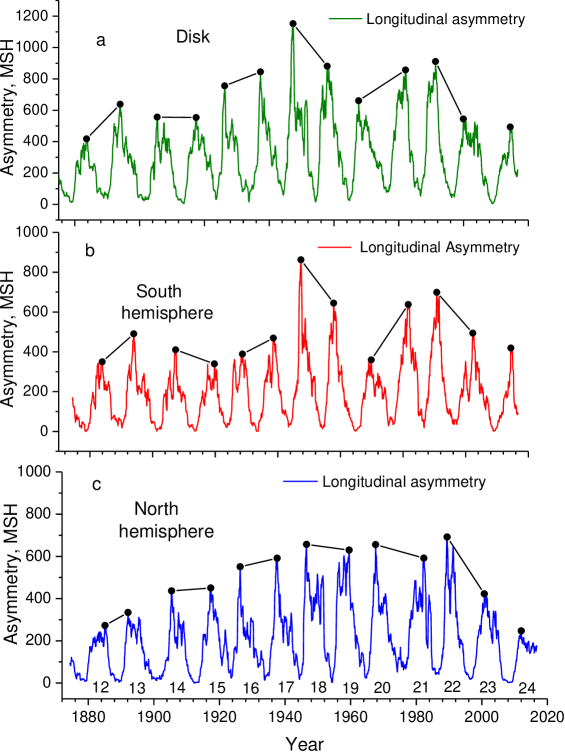
Figure 3.: Modulus of the longitudinal asymmetry vector for Solar Cycles 12–24 (1874–2016): (a) solar disk; (b) southern hemisphere; (c) northern hemisphere. Cycle numbers are shown at the bottom of the figure. Maxima of the even cycles ($2N$) and the following odd cycles ($2N+1$) are connected with straight line segments to emphasize the alternation of the cycle pairs following the Gnevyshev–Ohl rule or anti-Gnevyshev–Ohl rule. Curves were smoothed using 13-rotation running mean. lonasym

A common feature in the variation of the sunspot area (Figure area) and of the longitudinal asymmetry (Figure lonasym) is that they change in phase following the 11-year solar cycle. At the same time, a comparison of these two parameters show significant differences between them. The longitudinal asymmetry vector is 3-4 times smaller than the sunspot area due to reduced contribution of the stochastic component uniformly distributed over longitude. In the course of the cyclic changes the values of the LA do not always follow the changes of the sunspot area. Thus, Cycle 19 is the highest for the solar activity (Figure area), while for the LA the highest values are attained in Cycle 18 for the disc and for the southern hemisphere and in Cycle 22 for the northern hemisphere (Figure lonasym). In Cycle 20 the sunspot area was low for the disc, the southern and the northern hemispheres, whereas this cycle has one of the highest values of the LA for the northern hemisphere.

This difference between the amplitudes of the sunspot area cycles (Figure area) and of the LA cycles (Figure lonasym) leads to the transformation of the Gnevyshev–Ohl rule in the latter case. The relation between maxima of the two successive cycles (the even and following odd cycles) is marked in Figure lonasym by the line segments.

Longitudinal asymmetry of the sunspot distribution shows the following structure. Only the first pair of each four cycles followed the Gnevyshev–Ohl rule (the amplitude of an even solar cycle is lower than the amplitude of the following odd cycle); the next pair followed the “anti-Gnevyshev–Ohl rule”, i.e. the even cycle (cycle $2N$) exceeded the following odd cycle (cycle $2N+1$). This is true for Solar Cycles 12–23. Possibly, this pattern is a manifestation of the 44-year periodicity of the solar activity or the double Hale cycle.

It should be noted that the 44-year pattern described above was observed for the whole solar disc (Figure lonasyma) and was especially pronounced in the southern hemisphere (Figure lonasymb). In the northern hemisphere (Figure lonasymc) for the modulus of the longitudinal asymmetry an essentially different pattern is seen for 12 solar cycles (Cycles 12–23). During the first 6 cycles (Cycles 12–13, 14–15, 16–17) the Gnevyshev–Ohl rule holds – an even solar cycle was lower than the following odd cycle. However, the next 6 cycles followed the anti-Gnevyshev–Ohl rule – an even cycle was higher than the following odd cycle. In the northern hemisphere (Figure lonasymc) the amplitude of the longitudinal asymmetry sharply decreased in the beginning and at the end of time interval under consideration (low values of the modulus of the vector of the LA in Cycles 12, 13, 23 and 24).

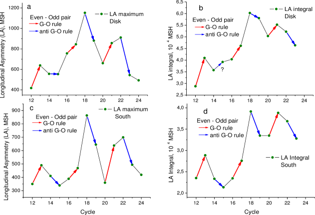
Figure 4.: (a,c) Maxima of the longitudinal asymmetry in Solar Cycles 12–24: (a) solar disk; (c) southern hemisphere. (b,d) Integral of the longitudinal asymmetry for individual solar cycles: (b) solar disk; (d) southern hemisphere. The red arrows show the pairs of even–odd cycles following the G-O rule. The blue arrows show the pairs of even–odd cycles following anti-G-O rule. In all of the cases (except one) the even-odd pairs show in turn the G-O rule or anti-G-O rule. maxint

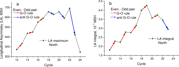
Figure 5.: Northern hemisphere in Solar Cycles 12–24: (a) Maximum of the longitudinal asymmetry. (b) Integral of the longitudinal asymmetry for individual solar cycles. The red arrows show the pairs of even–odd cycles following G-O rule. The blue arrows show the pairs of even–odd cycles following anti-G-O rule. In contrast to the disk and the southern hemisphere, the maxima of the longitudinal asymmetry in the northern hemisphere follow G-O rule only for Solar Cycles 12–17, while for Solar Cycles 18–23 anti-G-O rule holds. Integral of the longitudinal asymmetry changes in the same way as the area of sunspots (see Figure area2). north

3.2 Maximum and integral of the longitudinal asymmetry

S-Integral To show more clearly the alternation of high and low cycles, we considered the maxima of the longitudinal asymmetry for each of the cycles. Figure maxint shows the maximum of the LA values for the disk (Figure maxinta) and the southern hemisphere (Figure maxintc). To compare the heights of adjacent cycles in Figure maxint straight line segments were drawn connecting the maxima of even and subsequent odd solar cycles: the cases where the G-O rule holds are shown in red, the cases of the anti-G-O rule are marked by blue. It can be clearly seen that for the disc (Figure maxinta) and the southern hemisphere (Figure maxintc) there is an alternation of the G-O rule and the anti-G-O rule. These figures illustrate the main features of the variation of the modulus of the longitudinal asymmetry noted in the analysis of Figure lonasym. An interesting feature is the good correlation (correlation coefficient $R=0.86$) and an almost complete matching of the form of the dependencies for the disk (Figure maxinta) and for the southern hemisphere (Figure maxintc), for which the highest cycle of longitudinal asymmetry was Solar Cycle 18 and the second-largest cycle was Solar Cycle 22. For the solar disk and for the southern hemisphere, Solar Cycles 12, 15, 20 and 24 have the lowest height of the LA.

Similar to the research of Gnevyshev and Ohl (1948), where the integral characteristic of the solar cycle was used (the sum of Wolf numbers for each cycle), we considered the integral of longitudinal asymmetry calculated for each solar cycle. We considered the manifestation of the G-O rule for the longitudinal asymmetry integral whose variation in Solar Cycles 12–24 is shown in Figure maxintb (disc) and Figure maxintd (southern hemisphere).

The longitudinal asymmetry integral most clearly shows the alternation of the G-O rule and anti-G-O rule for the southern hemisphere (Figure maxintd.) There is one exception (the pair of Solar Cycles 14–15) for the disk.

It can be seen that the integral for the disc and for the southern hemisphere change in a similar manner, reaching the maximum in Solar Cycle 18 and the second maximum in Solar Cycle 21. On the whole, all four dependencies of Figure maxint resemble each other. The pair of cycles in which the G-O rule holds and the next pair obeying the anti-G-O rule form a stable pattern that repeats three times over the period in question.

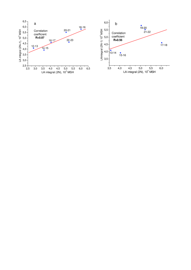
Figure 6.: Correlation of the longitudinal asymmetry maxima for the pairs of cycles: (a) an even cycle ($2N$) vs the following odd cycle ($2N+1$); correlation coefficient $R=0.87$. (b) an even cycle ($2N$) vs the previous odd cycle ($2N-1$); correlation coefficient $R=0.56$. corr

For the northern hemisphere, which behaves in a quite different way when compared to the disk and the southern hemisphere, the variation of the maximum and of the integral of longitudinal asymmetry in Solar Cycles 12–23 is shown in Figure north. In this case, the cycle maximum for longitudinal asymmetry follows the G-O rule for the first three cycle pairs, and for the next three cycle pairs the anti-G-O rule holds (Figure northa). High values of asymmetry maximum were observed in 6 consecutive cycles starting from Solar Cycle 17 to Solar Cycle 22, with the highest value of asymmetry in Solar Cycle 22. On the other hand, the integral of the longitudinal asymmetry of the northern hemisphere (Figure northb) follows the G-O rule in the same way as the area of sunspots (Figure area). As in the case of the sunspot area, the highest cycle is Solar Cycle 19. Thus, the integral of the LA for the northern hemisphere shows no distinctions from the usual sunspot area variation.

There exists the following formulation of the G-O rule (Gnevyshev and Ohl, 1948): the total Wolf number per even cycle (cycle $2N$) correlates well with the subsequent odd cycle (cycle $2N+1$), forming a pair of even-odd cycle (correlation coefficient $R=0.91$). In contrast, the correlation of the even cycle (cycle $2N$) to the previous odd cycle (cycle $2N-1$) is weak ($R=0.5$). We verified whether this phenomenon takes place for the longitudinal asymmetry integral. Figures corra,b illustrate two types of relations of the LA integral: for even-odd (a) and for odd-even cycles (b). In the first case, the correlation coefficient equals $R=0.86$, while in the second case $R=0.56$. These values are close to those obtained in (Gnevyshev and Ohl, 1948). It should be emphasized that the coincidence of the results was obtained despite the fact that essentially different parameters were considered (the sum of Wolf numbers per cycle and the integral of longitudinal asymmetry), as well as different time intervals (1700–1945 and 1874–2016, respectively). This supports the conclusion of Gnevyshev and Ohl (1948) that a pair of even and subsequent odd cycles form a joint structure.

It is known that large and small sunspots form two populations with different properties. E.g., it was shown in Nagovitsyn et al. (2018) that sunspots with area $Sp>50$ and $Sp<50$ MSH have different times of life and different latitude distributions. In Figure lonasym, the changes of the longitudinal asymmetry for the sunspots of arbitrary area were presented. The longitudinal asymmetry for the sunspots with area smaller than 50 MSH is shown in Figure small. It is seen that the LA of small sunspots obeys the usual G-O rule, as well as the sunspot area does (Figure area). Thus, the features of the longitudinal asymmetry which manifest themselves in alternation of G-O rule and anti-G-O rule and the corresponding 44-year structure are characteristic for long-living sunspots with large area.

The presence of a 44-year periodicity was observed in various parameters of the solar activity. For example, regular drops of the equatorial rotation rate of the Sun were found (Javaraiah, 2003) with a time gap of 44 years. This effect was interpreted as a manifestation of a double Hale cycle. The analysis of the large sunspot group diameters (Efimenko and Lozitsky, 2018) also shows the 44-year period in the variations of solar activity. There are some indications that the 44-year periodicity of solar activity is reflected in cosmic ray intensity. The study of connection between the solar activity and cosmic ray modulation showed that dimensions of the modulation region change not only with 11 and 22 year periods, but also with a period of 44 years (Dorman et al., 1999).

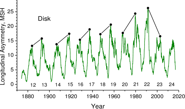
Figure 7.: Small sunspots (area $Sp<50$ MSH). Modulus of the longitudinal asymmetry vector for the solar disk (1874–2016) changes in the same way as the sunspot area (see Figure 2). Curves were smoothed using 13-rotation running mean. small

4 Active longitudes (phase of the longitudinal asymmetry vector)

S-Phase Asymmetry of the distribution of the solar activity over the heliolongitude manifests itself in the form of the so-called active or preferred longitudes. In this section the extension of our previous works on the problem of active longitudes (Vernova et al., 2004; Vernova, Tyasto and Baranov, 2005; Vernova, Tyasto and Baranov, 2007) is presented. Only large sunspots ($Sp>100$ MSH) were considered in this section. The longitudinal distribution of sunspots for 13 solar cycles (1874–2016) is shown in Figure nopref. The distribution over longitude is almost uniform and gives no evidence for the presence of preferred longitudes. However, the picture changes drastically if we study different periods of the solar cycle separately. In (Vernova et al., 2004) it was found that the distributions of sunspots over longitude have similar forms for the periods of the ascent and maximum on one hand and for the descent and minimum on the other hand. Therefore, in our analysis these parts of the cycle were considered jointly as the ascent-maximum epoch (AM) and the descent-minimum epoch (DM).

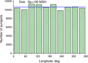
Figure 8.: Longitudinal distribution of the sunspot area ($Sp>100$ MSH) for 13 solar cycles (1874–2016). No preferred longitudes can be seen. nopref

The two characteristic periods (AM and DM) are connected with the magnetic cycle of the Sun. The boundaries of these characteristic periods coincide with the change of the polar field sign and the change of the leading sunspot sign in a hemisphere. Thus AM period corresponds to the interval from the solar minimum to the polar field reversal and DM – to the interval from the reversal to the minimum.

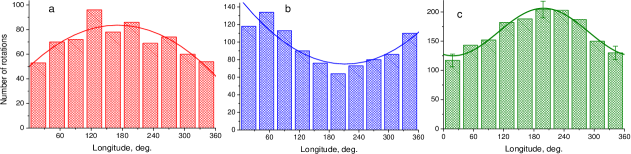
Figure 9.: Distribution of the phase of the longitudinal asymmetry vector for 13 solar cycles (1874–2016). (a) AM phase of the solar cycles. (b) DM phase; maximum of the distribution moves by $180^{\circ}$ during the transition from AM to DM phase and vice versa (flip-flop effect). (c) Joint distribution for AM and DM phases obtained by summing the AM histogram with the DM histogram shifted by $180^{\circ}$. Enveloping curve – approximation with a 2nd degree polynomial. phase

As stated above, the vector summing of the sunspot data allows us to separate the nonaxisymmetric component from the axisymmetric part of solar activity, which is distributed uniformly over the longitude. This method proved to be useful when studying the time variation of the longitudinal asymmetry (Section S-Asymmetry). For each Carrington rotation the phase of the longitudinal asymmetry vector points to the active longitude where large long-living sunspots were observed. If the vector of the longitudinal asymmetry has small magnitude then the value of the phase angle becomes unreliable. Therefore while investigating the longitudinal asymmetry we took into account only those cases where the modulus of the vector exceeded 20 MHS.

Distributions of the phase angle over the longitude for 1874–2016 are plotted in Figure phase for two periods, AM and DM, separately. These histograms display two forms of the enveloping curves: convex or concave. Corresponding maxima of distribution are located at longitudes $\sim 180^{\circ}$ for ascent-maximum (a) and $\sim 0^{\circ}/360^{\circ}$ for descent-minimum (b). Comparison of Figures phasea and Figures phaseb shows that there are two similar distributions with the shift of $180^{\circ}$ with respect to each other. We combined both histograms plotting the sum of histogram (a) with the histogram (b) shifted by $180^{\circ}$. Resulting histogram (Figure phasec) includes data of the whole interval under study (1874–2016). As an enveloping curve for the resulting histogram a sinusoidal function of the following form was chosen:

$$\ilabel{Eq-Hist}y=A\sin((x-B)/w)+C$$ (2)

Clearly displayed maximum of the envelope supports the idea of the active longitude jumping by $180^{\circ}$ (so-called flip-flop) at the boundaries between AM and DM periods. Stability of the longitude asymmetry maximum during 13 solar cycles can be interpreted as evidence of the rigid rotation of active longitudes.

If we use for the phase of solar cycle the following notation: $k=1$ corresponds to the period of 11-year cycle from the minimum to the polar magnetic field reversal; $k=2$ corresponds to the period from the reversal to the minimum, then the location of the distribution maximum (the active longitude) can be represented by the formula:

$$\ilabel{2}Active\,\,Longitude=\pi k$$ (3)

From the solar activity minimum to the reversal of the polar field (the AM period, active longitude $180^{\circ}$) the sign of the polar magnetic field and the sign of leading sunspots in a hemisphere coincide, while for the period from the reversal to the solar minimum (the DM period, active longitude $\sim 0^{\circ}/360^{\circ}$) these polarities are opposite.

5 Conclusions

S-Conclusions

Introducing the notion of the longitudinal asymmetry vector we evaluated the nonaxisymmetric part of the solar activity distribution. This approach allowed to reduce the influence of the stochastic component of the solar activity uniformly distributed over longitude and separate the stable nonaxisymmetric component. The change in the longitudinal asymmetry of the sunspot distribution was analyzed for the period of 13 solar cycles (1874–2016). The study of the nonaxisymmetric component of solar activity showed, on the one hand, a close connection of this component with the development of the solar cycle. On the other hand, significant features of longitudinal asymmetry have been found. In the longitudinal asymmetry of sunspot distribution for the disc and for the southern hemisphere in each four subsequent cycles (from Solar Cycle 12 to Solar Cycle 23) only for the first pair of cycles the Gnevyshev–Ohl rule held, while the next pair obeyed the ‘anti-rule’, i.e., the amplitude of an even cycle was higher than the amplitude of the next odd one. Possibly, this is a manifestation of a 44-year structure of solar activity.

For the northern hemisphere the Gnevyshev–Ohl rule holds for Solar Cycles 12–17, while for Solar Cycles 18–23 the anti-rule can be observed. The longitudinal asymmetry for sunspots with area $Sp<50$ MSH follows the Gnevyshev–Ohl rule similar to the sunspot area. Thus, the alternation of the Gnevyshev–Ohl rule and anti-Gnevyshev–Ohl rule is characteristic for large long-living sunspots.

The longitudinal asymmetry integral obeys the pattern found in (Gnevyshev and Ohl, 1948): the high correlation of the even $(2N)$ and the subsequent odd cycle $(2N+1)$ is accompanied by the low correlation of the even cycle $(2N)$ and preceding odd cycle $(2N-1)$.

The longitudinal distribution of the sunspot area for the period of 13 solar cycles does not show the presence of preferred longitudes. The concentration of solar activity on certain longitudes can be observed when the phase of the longitudinal asymmetry vector is considered for the periods ascent-maximum and descent-minimum separately. Then it becomes evident that the phase of the vector has the maximum at the longitude $180^{\circ}$ during the ascent-maximum epoch and at the longitude $0^{\circ}/360^{\circ}$ during the descent-minimum epoch. A drastic change of the active longitude by $180^{\circ}$ (flip-flop) occurs near the solar activity minimum and at the Sun’s global field reversal. The active longitude changes with the reversals of polarity of the local and global magnetic fields.

Acknowledgments

We thank the staff of the RGO/USAF/NOAA and personally Dr. David H. Hathaway for providing the homogeneous set of the sunspot data.

Disclosure of Potential Conflicts of Interest: The authors declare that they have no conflicts of interest

References

- Babcock (1961) Babcock, H.W.: 1961, Astrophys. J., 133, 572. ADS, DOI.
- Bai (1988) Bai, T.: 1988, Astrophys. J., 328, 860. ADS, DOI.
- Bai (2003) Bai, T.: 2003, Astrophys. J., 585, 1114. ADS, DOI.
- Balthasar and Schüssler (1983) Balthasar, H., Schüssler, M.: 1983, Solar Phys., 87, 23. ADS, DOI.
- Benevolenskaya et al. (1999) Benevolenskaya, E. E., Hoeksema, J. T., Kosovichev, A. G., Scherrer, P. H.: 1999, Astrophys. J., 517, L163. ADS, DOI.
- Benevolenskaya and Kostuchenko (2013) Benevolenskaya, E.E., Kostuchenko, I.G.: 2013, J. of Astrophys., 2013 Article ID 368380. DOI.
- Berdyugina and Usoskin (2003) Berdyugina, S. V., Usoskin, I. G.: 2003, Astron. Astrophys., 405, 1121. ADS, DOI.
- Bigazzi and Ruzmaikin (2004) Bigazzi, A., Ruzmaikin, A.: 2004, Astrophys. J., 604, 944. ADS, DOI.
- Bumba and Howard (1969) Bumba, V., Howard, R.: 1969, Solar Phys., 7, 28. ADS, DOI.
- Bumba et al. (1996) Bumba, V., Klvan̆a, M., Kálmán, B., and Garcia, A.: 1996, Astron. Astrophys. Suppl. Ser., 117, 291. ADS
- Charbonneau (2010) Charbonneau, P.: 2010, Living Rev. Solar Phys. 7, 3. ADS. DOI.
- de Toma, White, and Harvey (2000) de Toma, G., White, O. R., Harvey, K. L.: 2000, Astrophys. J., 529, 1101. ADS, DOI.
- Dodson and Hedeman (1968) Dodson, H. W., Hedeman, E. R.: 1968, in K. O. Kiepenheuer (ed.), Structure and Development of Solar Active Regions, IAU Symp., 35, 56. ADS
- Dorman et al. (1999) Dorman, L. I. Dorman, I.V., Iucci, N., Parisi, M., Villoresi G. : 1999, Proc. 26th Int. Cosmic Ray Conf. , 7,198. ADS.
- Efimenko and Lozitsky (2018) Efimenko, V.M., Lozitsky, V.G.: 2018, Adv. Space Res. 61, 2820. ADS, DOI.
- Gaizauskas et al. (1983) Gaizauskas, V., Harvey, K. L., Harvey, J. W., Zwaan, C.: 1983, Astrophys. J., 265, 1056. ADS, DOI.
- Gaizauskas (1993) Gaizauskas, V.: 1993 in H. Zirin, G. Ai, and H. Wang (eds.), The magnetic and velocity fields of solar active regions, ASP Conference Series, 46, 479. ADS
- Gnevyshev and Ohl (1948) Gnevyshev, M.N., Ohl, A. I.: 1948, In Russian Astron. J. 25, 18.
- Javaraiah (2003) Javaraiah, J.: 2003, Solar Phys. 212, 23. ADS, DOI.
- Javaraiah (2013) Javaraiah, J.: 2013, Adv. Space Res. 52, 963. ADS, DOI.
- Javaraiah (2016) Javaraiah, J.: 2016, Astrophys. Space Sci. 361, 208. ADS, DOI.
- Jetsu et al. (1997) Jetsu L., Pohjolainen S., Pelt J., Tuominen I.: 1997, A&A. 318, 293. ADS.
- Leighton (1969) Leighton, R.B.: 1969, Astrophys. J., 156, 1. ADS, DOI.
- Nagovitsyn, Nagovitsyna and Makarova (2009) Nagovitsyn, Y.A., Nagovitsyna, E.Y., Makarova, V.V.: 2009, Astron. Lett. 35, 564. ADS, DOI.
- Nagovitsyn et al. (2018) Nagovitsyn, Y.A., Pevtsov, A.A., Osipova, A.A., Ivanov, V.G.: 2018, Geomagn. Aeron. 58, 1170. ADS, DOI.
- Neugebauer et al. (2000) Neugebauer, M., Smith, E. J., Ruzmaikin, A., Feynman, J., and Vaughan, J. H.: 2000, J. Geophys. Res., 105, 2315. ADS, DOI.
- Ogurtsov (2012) Ogurtsov, M. G.: 2012, Geomagnetism and Aeronomy, 52, 977. ADS, DOI.
- Pipin and Kosovichev (2015) Pipin V.V., Kosovichev A.G.: 2015, Astrophys. J., 813, ID 134. ADS. DOI.
- Pipin et al. (2019) Pipin, V.V., Pevtsov, A.A., Liu, Y., Kosovichev, A.G.: 2019, Astrophys. J. Lett. 877, L36. ADS
- Ruzmaikin (2001) Ruzmaikin, A.: 2001, Space Sci. Rev., 95, 43. ADS.
- Skirgiello (2005) Skirgiello, M.: 2005, Ann. Geophys., 23, 3139. ADS, DOI.
- Tuominen, Berdyugina and Korpi (2002) Tuominen, I., Berdyugina, S.V., Korpi, M.J.: 2002, Astronomische Nachrichten 323, 367. ADS, DOI.
- Vernova et al. (2002) Vernova, E. S., Mursula, K., Tyasto, M. I., Baranov, D. G.: 2002, Solar Phys., 205, 371. ADS, DOI.
- Vernova et al. (2004) Vernova, E.S., Mursula, K., Tyasto, M.I., Baranov, D.G.: 2004, Solar Phys. 221, 151. ADS, DOI.
- Vernova, Tyasto and Baranov (2005) Vernova, E.S., Tyasto, M.I., Baranov, D.G.: 2005, Memorie della Societa Astronomica Italiana 76, 1052. ADS
- Vernova, Tyasto and Baranov (2007) Vernova, E.S., Tyasto, M.I., Baranov, D.G.: 2007, Solar Phys. 245, 177. ADS, DOI.