Training Object Detectors from Few Weakly-Labeled and Many Unlabeled Images

Abstract

Weakly-supervised object detection attempts to limit the amount of supervision by dispensing the need for bounding boxes, but still assumes image-level labels on the entire training set. In this work, we study the problem of training an object detector from one or few images with image-level labels and a larger set of completely unlabeled images. This is an extreme case of semi-supervised learning where the labeled data are not enough to bootstrap the learning of a detector. Our solution is to train a weakly-supervised student detector model from image-level pseudo-labels generated on the unlabeled set by a teacher classifier model, bootstrapped by region-level similarities to labeled images. Building upon the recent representative weakly-supervised pipeline PCL [1], our method can use more unlabeled images to achieve performance competitive or superior to many recent weakly-supervised detection solutions. Code will be made available at https://github.com/zhaohui-yang/NSOD.

Licensed CC-BY-NC-ND 2.0

1 Introduction

The objective of visual object detection is to place a tight bounding box on every instance of an object class. With the advent of deep learning, recent methods [2, 3, 4, 5] have significantly boosted the detection performance. Most are fully supervised, using a large amount of data with carefully annotated bounding boxes. However, annotating bounding boxes is expensive.

To reduce the amount of supervision, the most common setting is weakly-supervised object detection (WSOD) [6, 7, 8, 9]. In this setting, we are given a set of images known to contain instances of certain classes as specified by labels, but we do not know the object locations in the form of bounding boxes or otherwise. Many works [10, 7, 11, 12] formulate weakly supervised object detection as multiple instance learning (MIL) [13], which has been extended to be learnable end-to-end [6, 8].

There are mixed approaches where a small number of images are annotated with bounding boxes and labels, and a large amount of images have only image-level labels [14, 15, 16]. This is often referred as a semi-supervised setting [14, 16, 17], but there is no consensus.

Semi-supervised learning [18] refers to using a small amount of labeled data and a large amount of unlabeled data. It is traditionally studied for classification [19, 20, 21], with one class label per image and no bounding boxes. In object detection, this would normally translate to a small number of images having labels and bounding boxes, and a large number of images having no annotation at all. This problem has been studied for the case where the fully annotated data (with bounding boxes) are enough to train a detector in the first place [22, 23], resulting in two-stage learning. But what if these data are very scarce?

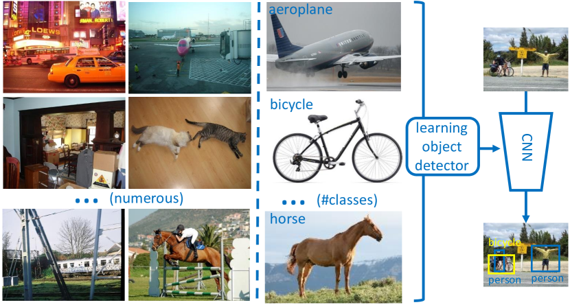
Figure 1: We learn an object detector from a set of completely unlabeled images and one or few images per class with image-level label per image and no other information.

In this work, we study object detection in the challenging setting where only one or few images per class are given with only image-level class label per image, and a large amount of images with no annotation at all. We use no bounding boxes or other information. This setting is illustrated in Fig. 1. Some initial exploration can be found in [24, 25, 26] before deep learning. The few weakly-labeled images can be obtained via either labeling images from an unlabeled collection [24, 25] or using the top-ranking images from web image search with the class name as the query [26]. Both paradigms are studied in our work. The latter is preferable as it requires no human effort.

Our deep learning solution is called nano-supervised object detection (NSOD). It begins by computing region-level class scores based on the similarity between the unlabeled images and the few weakly-labeled images, which we then pool into image-level class probabilities. This yields image-level pseudo-labels on the entire unlabeled set, which we use to train a teacher model on a classification task. Then, by predicting new image-level multi-class pseudo-labels on the unlabeled set, we train a student model on a detection task, using a weakly-supervised object detection pipeline.

Contributions. We study the very challenging problem of training an object detector from few images with only image-level labels and many images with no annotation at all. We introduce a new method for this problem that is simple, efficient (cost comparable to standard WSOD), and modular (can build on any WSOD pipeline). By using the recent pipeline of PCL [1] and more unlabeled images, we achieve performance competitive or superior to many recent WSOD solutions. On PASCAL VOC 2007 test set for instance, using 20 web images per class, we get a detection mAP of 42, compared to 43.5 of PCL, which is using image-level labels on the entire training set.

2 Related Work

2.1 Weakly supervised object detection (WSOD).

In this setting, all training images have image-level class labels. A classic approach is multiple instance learning (MIL) [13], considering each training image as a “bag” and iteratively selecting high-scoring object proposals from each bag, treating them as ground truth to learn an object detector.

Bilen and Vedaldi [6] introduce weakly-supervised deep detection network (WSDDN), which pools region-level scores into image-level class probabilities and enables end-to-end learning from image-level labels. Concurrently, Tang et al. [27] introduce a deep convolutional neural network by integrating traditional multiple instance learning (MIL) into it for end-to-end training. Furthermore, Tang et al. [8] extend WSDDN to multiple instance detection network with an online instance classifier refinement (OICR) scheme and introduce a weakly-supervised region proposal network as a plugin [28]. In proposal cluster learning (PCL) [1], pre-clustering of object proposals followed by OICR accelerates learning and boosts performance. In [29], a pseudo ground truth mining algorithm is also introduced to improve OICR. Recently, Zeng et al. [30] propose a novel WSOD framework with objectness distillation by jointly considering bottom-up and top-down objectness from low-level measurement and CNN confidences with an adaptive linear combination. Ren et al. [9] employ an instance-aware self-training strategy for WSOD with Concrete DropBlock. Zhang et al. [31] extract the category-aware spatial information from a classification network to both classify and localize objects using image-level annotation. Liu et al. [32] leverage a graph neural network into WSOD to discover semantic label co-occurrence.

Besides improvements in the network architecture, there are also attempts to incorporate additional cues into WSOD that are still weaker than bounding boxes, e.g. object size [7] and count [33]. It is also common to use extra data to transfer knowledge from a source domain and help localize objects in the target domain [34, 35]. Large-scale weakly-labelled web images [36, 37] and videos [38, 39] with noisy labels are also common as extra data.

Our problem is different from WSOD in that the few labeled images have no bounding boxes and the bulk of the training set is completely unlabeled. We build our work on PCL [1] but train it with image-level pseudo-labels.

2.2 Semi-supervised learning.

There are several works that assume a few images are annotated with object bounding boxes and the rest still have image-level labels as in WSOD [14, 15, 16]. These are often called semi-supervised [14, 16, 40, 41, 42]. However, semi-supervised may also refer to the situation where some images are labeled (at image-level or with bounding boxes) and the rest have no annotation at all [22, 23]. This situation is consistent with the standard definition of semi-supervised learning [18]. Despite advances in deep semi-supervised learning [43, 44, 45], most work focuses on classification tasks. In pseudo-label [20] for instance, classifier predictions on unlabeled data are used as labels along with true labels on labeled data. Few exceptions focusing on object detection [22, 23, 46, 42] still assume enough labeled images to learn a detector in the first place, which is not the case in our work.

Tang et al. [46] assume part of the training set is strongly labelled with bounding boxes and the other part is unlabelled. They also call this setting semi-supervised. They experiment on large labeled and unlabeled sets (118K and 123K respectively in COCO): the labeled data is trained in a standard Faster R-CNN, while for the unlabeled data, a self-supervised proposal learning module and a consistency-based proposal learning module are introduced. Gao et al. [42] assume a few seed training images are annotated with bounding boxes and the rest are weakly labeled with image-level annotations. This is again called semi-supervised. The seed samples are trained with Faster R-CNN while an iterative training-mining pipeline is introduced to mine bounding boxes from the weakly-labelled set for joint training.

The supervision settings of Tang et al. [46] and Gao et al. [42] are different, but in both cases, the labelled data are enough to bootstrap a standard Faster R-CNN. This is not the case in our work. Dong et al. [47] use few images with object bounding boxes and class labels along with many unlabeled images. However, this method relies on several models (i.e. Fast R-CNN, R-FCN, SPL) and iterative training, which is computationally expensive.

Our problem can be considered as an extreme case of semi-supervised object detection: the labeled images are very few and with only image-level labels, which is too little to learn a good detector like Faster R-CNN. We thus introduce a nano-supervised solution with teacher-student distillation. Shi et al. [24] also use a mixture of few weakly-labeled images and unlabeled images for object detection. Their method involves hand-crafted features and iterative message passing, which would not be straightforward or efficient to extend to a deep learning framework.

It should be noted that Gao et al. [42] also employ a teacher model in their pipeline, but the teacher is an object detector pre-trained on a large amount of fully-labelled images on source classes. This provides additional help against the noisy labels in the bounding box mining process. By contrast, our teacher comes from a model pre-trained on ILSVRC classification, which is the most easily and widely accessed model for the majority of computer vision tasks. Thanks to our careful design of knowledge distillation, our approach also turns out to be effective and robust to noisy labels.

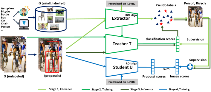
Figure 2: Overview of our nano-supervised object detection (NSOD) framework. We are given a support set $G$ and a large unlabeled set $X$. $G$ contains one or few weakly-labeled images per class, obtained from the web or randomly labeled from $X$. Using the images in $G$ and a feature extractor pre-trained on classification, we infer image-level class probabilities of images in $X$ (stage 1). We then extract pseudo-labels on $X$ and train a teacher network $T$ on a $C$-way classification task (stage 2). $T$ is used to classify each proposal of images in $X$, resulting in new image-level class probabilities (stage 3). We average these with the ones obtained in stage 1, based on $G$. Finally, we extract multi-class pseudo-labels on $X$ and train a student network $U$ on weakly-supervised detection by PCL [1] (stage 4).

2.3 Curated data.

Investigation of unsupervised settings relies on removing the labels from labeled datasets by default. This is the case e.g. for object discovery [48, 49], semi-supervised classification [50] and crowd counting [51, 52] until today. Such datasets are curated, i.e., still depict the same classes and are more or less balanced. Working with unknown classes is a different problem of open-set recognition [53]. At very large scale, keeping the top-ranking examples according to predicted class scores may be enough to address this problem [54]. We experiment on both curated and unlabeled data in the wild to show the robustness of our method.

3 Method

3.1 Preliminaries

Problem. We are given a support set $G$ containing $k$ images per class, each associated with an image-level label over $C$ classes. We are also given an unlabeled set of images $X$, where each image depicts one or more instances of the $C$ classes, along with background clutter. In a harder setting, images in $X$ may depict zero or more instances of the $C$ classes, along with instances of unknown classes or background clutter. There is no bounding box or any other information in either $G$ or $X$. Using these data and a feature extractor $\phi$ pre-trained on classification, the problem is to learn a detector to recognize instances of the $C$ classes and localize them with bounding boxes in new images.

Motivation. This problem relates to both weakly-supervised detection and semi-supervised classification. Similar to the former, we study multiple instance learning but without image-level labels in the unlabeled set. Unlike the latter, at least in its common setting where thousands of examples are used [21, 44], $G$ is too small to bootstrap the learning of a good classifier or detector: $k$ can be as few as one example per class. For this reason, we propagate labels from $G$ to $X$ to initiate training.

Method overview. As shown in Fig. 2, we begin by collecting the support set $G$ (Sec. 4.1). We extract object proposals [55] from images in $X$ and compare region-level features obtained by a feature extractor $\phi$ against global features on $G$. We estimate class probabilities on $X$ by propagating these similarities to image level (stage 1, Sec. 3.2). We infer pseudo-labels on $X$ and train a teacher network $T$ inherited from $\phi$ on a $C$-way classification task (stage 2, Sec. 3.3). We use $T$ to classify regions in images of $X$, resulting in new image-level class probabilities (stage 3), which we average with the ones of stage 1. Finally, we infer multi-class pseudo-labels on $X$ and train a student network $U$ on a WSOD task by PCL [1] (stage 4).

Collecting the support set $G$. The support set can be obtained either by random selection from some existing dataset or by web image search. The latter is preferable as we would like images to be clean, e.g. depicting only one class per image. We experiment with both options.

3.2 Inferring class probabilities on $X$

Given the support set $G$ and corresponding labels, we begin by propagating the label information from $G$ to the unlabeled set $X$. For each image $\mathbf{x}$ in $X$, we use edge boxes [55] to extract a collection of $R$ object proposals (regions). Ideally, we would like to have one label per region so we can train an object detector. Since the supervision in our case is very limited, it is not realistic to assign an accurate label per region based only on $G$. Instead, it is more reliable to estimate image-level class probabilities on $X$. Inspired by the two-stream CNN architecture of WSDDN [6], we introduce a new way to infer image-level probabilities on $X$, by aggregating region-level class probabilities.

Similarity. We extract a feature vector $\phi(\mathbf{r})$ for each region $\mathbf{r}$ of image $\mathbf{x}$. We do the same for each image $\mathbf{g}$ in $G$, extracting a feature vector $\phi(\mathbf{g})$. This is a global feature vector. Let $G_{j}$ be the support images labeled as class $j$, with $\left|{G_{j}}\right|=k$. Let also $\mathbf{r}_{i}$ be the $i$-th region of $\mathbf{x}$. We define the $R\times C$ similarity matrix $S=\{s_{ij}\}$ with elements

$$s_{ij}\mathrel{:=}\frac{1}{k}\sum_{\mathbf{g}\in G_{j}}c(\phi(\mathbf{r}_{i}),\phi(\mathbf{g})),$$ (1)

where $c$ denotes cosine similarity.

Voting. Inspired by [6], we form $R\times C$ classification matrix $\sigma_{\mathrm{cls}}(S)$ with each row being the softmax of the same row of $S$, implying competition over classes per region; similarly, we form $R\times C$ detection matrix $\sigma_{\mathrm{det}}(S)$ with each column being the softmax of the same column of $S$, implying competition over regions per class:

$$\sigma_{\mathrm{cls}}(S)_{ij}\mathrel{:=}\frac{e^{s_{ij}}}{\sum_{j=1}^{C}e^{s_{ij}}},\quad\sigma_{\mathrm{det}}(S)_{ij}\mathrel{:=}\frac{e^{s_{ij}}}{\sum_{i=1}^{R}e^{s_{ij}}}.$$ (2)

The $i$-th row of $\sigma_{\mathrm{cls}}(S)$ expresses a vector of class probabilities for region $\mathbf{r}_{i}$, while the $j$-th column of $\sigma_{\mathrm{det}}(S)$ a vector of region probabilities (spatial distribution) for class $j$.

The final image-level class scores ${\boldsymbol{\sigma}}(S)$ are obtained by element-wise product of $\sigma_{\mathrm{cls}}(S)$ and $\sigma_{\mathrm{det}}(S)$ followed by sum pooling over regions

$${\boldsymbol{\sigma}}(S)_{j}\mathrel{:=}\sum_{i=1}^{R}\sigma_{\mathrm{cls}}(S)_{ij}\sigma_{\mathrm{det}}(S)_{ij}.$$ (3)

Each score ${\boldsymbol{\sigma}}(S)_{j}$ is in $[0,1]$ and can be interpreted as the probability of object class $j$ occurring in image $\mathbf{x}$.

Discussion. The above is a robust voting strategy which propagates proposal-level information to the image level, while suppressing noise. Formula (1) suggests that region $\mathbf{r}_{i}$ will respond for class $j$ if it is similar to any of the support images in $G_{j}$. While this response is noisy since it is only based on a few examples, it is only maintained if it is among the strongest over all classes and all regions in an image. Note that in [6], softmax is applied to two separate data streams during learning, whereas it is applied to the same matrix in our work.

Alternative ways to transfer label information from $G$ to $X$ would be to directly learn a parametric classifier on $G$ or define a nearest-neighbor classifier on $G$ and infer image-level labels on $X$. We consider such baselines in our experiments. Their performance is not satisfactory, which highlights the importance of robustly propagating labels from region to image level.

3.3 Teacher and student training

Having class probability vectors (3) per image in $X$, a next step would be to convert them to multi-class pseudo-labels and train the student directly on a weakly-supervised detection task. Nevertheless, probabilities generated this way rely on the few support images in $G$ for classification, while the object information in the unlabeled set $X$ is not exploited. To further enhance performance, we use distillation [56, 23] to transfer knowledge between data (labeled to unlabeled) and models (classification to detection). In particular, we distill knowledge from the support set $G$ to the unlabeled set $X$ using a teacher classifier $T$, and then distill this knowledge from the teacher to a student detector $U$.

Data distillation. We form the teacher $T$ as the feature extractor network $\phi$ followed by a randomly initialized $C$-output fully-connected layer and softmax. We then fine-tune $T$ on a $C$-way classification task on $X$. The probabilities (3) are meant for multi-label classification ($C$ independent binary classifiers), while here we are learning a single $C$-way classifier, i.e. for mutually exclusive labels. Given the class probability vector ${\boldsymbol{\sigma}}(S)$ for each image $\mathbf{x}$ in $X$, we take the most likely class $\arg\max_{j}{\boldsymbol{\sigma}}(S)_{j}$ as a $C$-way pseudo-label. We fine-tune $T$ on these pseudo-labels with a standard cross-entropy loss.

We have also tried several multi-label variants [57, 58], which are inferior to the simple $C$-way cross-entropy loss in our experiments. This may be attributed to the class sample distribution in $X$ being unbalanced.

Knowledge distillation. The fine-tuned teacher $T$ encodes object information of $X$ into its network parameters. Directly using its image-level predictions on $X$ would not be appropriate to train the student $U$ for detection, because the latter would need multi-class labels. On the other hand, using it as feature extractor to repeat the process of Sec. 3.2 would not make much difference either, as it still produces class probabilities based on $G$. Instead, we use $T$ to directly classify object proposals in $X$. Each proposal ideally contains one object, so it is particularly suitable to use $T$ as it was designed: a $C$-way classifier.

Given an input image $\mathbf{x}$ in $X$, we collect output class probabilities of $T$ on each region $\mathbf{r}_{i}$ of $\mathbf{x}$ into a $R\times C$ matrix $A$ with element $a_{ij}$ being the probability of class $j$. From this matrix, it is possible to estimate new image-level class probabilities by ${\boldsymbol{\sigma}}(A)$, similar to (3). Because it is based on $T$ being trained on $X$ as classifier, while ${\boldsymbol{\sigma}}(S)$ (3) is based on $G$ alone, we combine their strength by averaging both into a probability vector

$$\hat{\mathbf{q}}\mathrel{:=}\frac{1}{2}\left({\boldsymbol{\sigma}}(S)+{\boldsymbol{\sigma}}(A)\right)$$ (4)

corresponding to image $\mathbf{x}$.

An image-level multi-class pseudo-label $\hat{\mathbf{y}}\in\{0,1\}^{C}$ is then obtained from $\hat{\mathbf{q}}$ by element-wise thresholding. An element $\hat{y}_{j}=1$ specifies that an object of class $j$ occurs in image $\mathbf{x}$. In the absence of prior knowledge or validation data, we choose $\frac{1}{2}$ as threshold. Importantly, an all-negative pseudo-label $\hat{\mathbf{q}}=(0,\dots,0)$ is possible, e.g. when an image does not depict any known class. This simple mechanism allows our method to work in the harder setting where images in $X$ may depict only unknown classes.

Those image-level pseudo-labels are all that is needed to obtain an object detector if we use any WSOD pipeline. In particular, we train the student model $U$ on weakly-supervised detection on $X$ using proposal cluster learning (PCL) [1]. Weakly-labeled images in $G$ are also included into the training with loss weight 1.

Inference. At inference, the teacher classifier is not needed. The trained student detector is used directly.

4 Experiments

4.1 Experimental setup

Unlabeled set $X$. We choose the standard object detection datasets PASCAL VOC 2007 and 2012 [59] for the unlabeled set, having 20 classes. Each dataset contains a trainval set and a test set. For VOC 2007, the trainval set has 5011 images and the test set 4952 images. For VOC 2012, the size of trainval and test sets are 11540 and 10991, respectively. We use the trainval sets as $X$ to train the object detector by default. We evaluate the detector on the test set. Importantly, except for the support set, we do not use any labels, not even image-level labels in the training set.

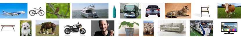
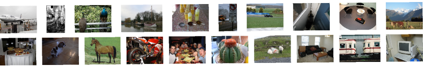
Figure 3: (Top) examples of top-ranking web images, using class names as queries. (Bottom) random selection of images from PASCAL VOC 2007.

Support set $G$. Each image in the support set $G$ should depict one of the known $C$ classes (i.e. 20 VOC classes). A preferable way to collect $G$ is from the web [26]: we use the class names as text queries and collect the top-$k$ results per class from web image search (e.g. Google). The motivation is that these images are clean, i.e. they mostly contain objects against a simple background and in a canonical pose and viewpoint, without clutter or occlusion (see examples in Fig. 3 (top)). Notwithstanding, they are not perfect, lacking diverse appearance and poses of the object class. Collecting images from the web is easy and does not need any human effort. We choose this option by default.

Another common option is to randomly sample $k$ images per class from an existing collection [24, 25] (e.g. VOC 2007). This is a harder setting, as these images may depict small objects, multiple instances, object classes in non-canonical pose, clutter and occlusion, e.g. bottle, chair, and person in Fig. 3 (bottom). We experiment with both options.

Networks. We choose VGG16 [60] as our student $U$ by default, which is consistent with most WSOD methods [6, 8, 28, 61, 1]. Since the teacher network $T$ (including the feature extractor $\phi$) is not used at inference time, we choose the more powerful ResNet-152 [62]. Both networks are pre-trained on the ILSVRC classification task [63].

Implementation details. We use $k=20$ images per class by default for $G$. Following representative WSOD methods [6, 8, 1, 64], we adopt edge boxes [55] to extract $2000$ proposals on average per image in $X$. For the default teacher model $T$, we first resize the input image to $256$ pixels on the short side and then crop it to $224\times 224$. We set the batch size to $128$ and the learning rate to $10^{-3}$ initially with cosine decay. For the default student model $U$, we feed the network with one image per batch. The training lasts for $50,000$ iterations in total; the learning rate starts at $10^{-5}$ and decays by an order of magnitude at $35,000$ iterations.

Method	aero	bike	bird	boat	bott	bus	car	cat	char	cow	tabl	dog	hors	mbik	prsn	plat	shep	sofa	tran	tv	mAP
NSOD	57.9	59.7	43.2	10.5	13.1	62.7	58.6	43.9	10.6	51.1	25.7	49.8	39.3	60.6	14.9	10.9	33.5	45.2	42.5	27.8	38.0
NSOD (07+12)	51.5	65.2	48.9	13.2	19.7	64.8	59.3	55.5	12.4	59.3	24.3	54.1	47.4	62.8	20.7	15.0	39.5	51.3	53.8	21.4	42.0
NS-FT	56.7	37.2	31.8	10.7	4.6	44.7	42.7	51.4	3.5	17.7	4.2	37.6	22.5	51.6	13.1	10.0	28.9	36.3	39.2	14.3	27.9
NS-NN	59.2	33.3	28.3	22.5	5.4	43.7	39.3	32.3	2.3	40.1	7.5	42.2	34.2	33.2	12.6	7.7	30.5	31.1	47.6	13.7	28.3
NS-MT-v1	49.6	33.9	29.6	15.5	9.5	47.9	32.9	49.1	0.2	13.2	21.1	34.4	19.7	31.5	9.6	9.9	35.6	43.1	38.9	15.0	27.0
NS-MT-v2	46.6	22.5	25.6	7.4	4.2	49.0	35.4	71.4	0.4	25.0	22.5	56.7	38.3	58.8	6.9	10.3	27.0	59.1	22.9	6.0	29.8
WSDDN [6]	39.4	50.1	31.5	16.3	12.6	64.5	42.8	42.6	10.1	35.7	24.9	38.2	34.4	55.6	9.4	14.7	30.2	40.7	54.7	46.9	34.8
OICR [8]	58.0	62.4	31.1	19.4	13.0	65.1	62.2	28.4	24.8	44.7	30.6	25.3	37.8	65.5	15.7	24.1	41.7	46.9	64.3	62.6	41.2
WSRPN [28]	57.9	70.5	37.8	5.7	21.0	66.1	69.2	59.4	3.4	57.1	57.3	35.2	64.2	68.6	32.8	28.6	50.8	49.5	41.1	30.0	45.3
PCL [1]	54.4	69.0	39.3	19.2	15.7	62.9	64.4	30.0	25.1	52.5	44.4	19.6	39.3	67.7	17.8	22.9	46.6	57.5	58.6	63.0	43.5
WS-JDS [61]	52.0	64.5	45.5	26.7	27.9	60.5	47.8	59.7	13.0	50.4	46.4	56.3	49.6	60.7	25.4	28.2	50.0	51.4	66.5	29.7	45.6

Table 1: Detection mAP on the test set of PASCAL VOC 2007. NSOD: our nano-supervised object detection framework; NS-FT: nano-supervised fine-tuning; NS-NN: nano-supervised nearest neighbor; NS-MT: Nano-supervised mean teacher. Unless otherwise stated, NSOD, NS-FT, NS-NN use $k=20$ support images per class by default. All compared methods [6, 8, 28, 1, 61] use the image-level labels in the unlabeled set $X$; NSOD, NS-FT, NS-NN and NS-MT do not.

Evaluation protocol. We evaluate the performance of our NSOD framework on both image classification and object detection. For image classification, we measure the average precision (AP) and mean AP (mAP) for multi-class predictions [57, 58], as well as the accuracy of the top-1 class prediction per image on the trainval set of $X$. For object detection, we quantify localization performance on the trainval set by CorLoc [6, 7, 8, 64] and detection performance on the test set by mAP. At test time, the detector can localize multiple instances of the same class per image and mAP is identical to what is used to evaluate fully supervised object detectors with an IoU threshold of 0.5. By using the same IoU threshold, we measure the recall rate of edge boxes over ground truth to be 92.51% and 91.27% on VOC 2007 and 2012 respectively. This shows the capacity of edge boxes to cover most ground truth regions.

Evaluation scenarios. Below, we first present the object detection results on the test set of $X$ under two scenarios: support set $G$ by web search (subsection 4.2) and by sampling VOC 2007 (subsection 4.3). Then in the ablation study (subsection 4.4), we provide detection and classification results on the trainval set of $X$ using the web search scenario.

4.2 Support set $G$ by web search

We first collect the support set by web search and evaluate our NSOD on both VOC 2007 and 2012. We also combine the two sets as well as images from ImageNet as distractors to evaluate our method in the wild.

4.2.1 Results on VOC 2007

Comparison to weakly-supervised methods. We compare to several representative WSOD methods [6, 8, 28, 1, 61] in Table 1. For fair comparison, all these methods use the same VGG16 backbone as we do, without bells and whistles. NSOD requires no annotation on the unlabeled set $X$, while weakly-supervised methods assume image-level labels for all images in $X$.

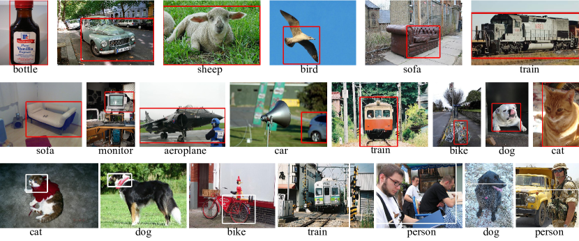
Figure 4: Detection results of NSOD on PASCAL VOC 2007, using default settings ($k=20$). Top 2 rows: positive results (red boxes). Bottom row: failure cases (white boxes).

One directly competing method is PCL trained on ground truth image-level labels in $X$. Despite using no annotation on $X$, NSOD achieves an mAP that is only 5.5% below that of PCL (38.0 vs. 43.5). The result is is also competitive to other methods, e.g. OICR [8], WSRPN [1]. There are also WSOD methods employing large-scale web images/videos as extra data. For instance, [37] and [38] build on the WSDDN pipeline [6] and produce mAP 36.8 and 39.4 on VOC 2007, respectively. Unlike these works, our NSOD uses few web images, an unlabeled set, and an advanced WSOD pipeline. Importantly, NSOD also delivers competitive mAP. Fig. 4 gives some examples of detection results of NSOD on PASCAL VOC 2007.

Comparison to semi-supervised methods. We first compare NSOD to two semi-supervised baselines: (1) fine-tune the teacher $T$ on $G$ as a $C$-way classifier and use it to make predictions on $X$, referred to as NS-FT; (2) use $\phi$ from $T$ as a global feature extractor to find the nearest neighbor in $G$ for each image in $X$, referred to as NS-NN. In both cases, we use the same support set with NSOD, infer image-level $C$-way pseudo-labels on $X$ and use them to train the student $U$ by PCL. As shown in Table 1, NS-FT and NS-NN deliver a mAP of 27.9 and 28.3, respectively. Comparing to the mAP 38.0 of NSOD on the same setting ($k=20$), these baselines are not satisfactory. This is due to the limited the supervision from the support set and justifies our choice of propagating labels from region to image level.

We then adapt the mean teacher [45] semi-supervised classification method to our setting. We use it in two ways: 1) using image-level class probabilities $\hat{\mathbf{q}}$  in Eq.(4), we select the top-$z$ scored images as positive for each class and the rest we treat as negative. With those pseudo-labels, we train PCL on VGG16, applying the consistency loss of [45] to image-level predictions on $X$. We call this nano-supervised mean teacher - variant 1 (NS-MT-v1). We choose $z=300$ as it works the best in practice. NS-MT then yields an mAP of 27.0 as shown in Table 1. This result is lower than our NSOD by 11.0% (27.0 vs. 38.0); 2) using the labeled support set $G$ and unlabeled set $X$, we train the teacher model $T$ as a mean-teacher by applying the cross-entropy loss on G and consistency loss between G and X. The rest pipeline remains as in NOSD. We name this nano-supervised mean teacher - variant 2 (NS-MT-v2) and obtain an mAP of 29.8 vs. 38.0 of NSOD. Both variants of NS-MT are clearly inferior to NSOD, which suggests that it is not straightforward to transfer a successful semi-supervised approach from the classification to the detection task.

We have also tried to directly infer object bounding boxes on the test set of VOC 2007 using naive approaches. In particular:

1. We use the $C$-way classifier $T$ trained on $X$ (stage 3) to directly predict the class probabilities of object proposals per image in the test set.

2. We adopt a naive $k$-NN classifier by computing the feature similarities from images in the support set $G$ to the object proposals per image in the test set.

The mAP in both cases can be measured by ranking the proposals by their class probabilities. These methods fail, producing mAP lower than 10. We should emphasize the importance of propagating similarity scores from region-level to image-level as we do in NSOD.

4.2.2 Results on VOC 2012

Using the same support set $G$, we train an object detector with our NSOD on VOC 2012. The mAP is reported on the test set of VOC 2012 and compared to representative WSOD methods [8, 1, 64] in Table 2. Despite not using any VOC 2012 labels, NSOD is only 4.0% below PCL (36.6 vs. 40.6).

Method	aero	bike	bird	boat	bott	bus	car	cat	char	cow	tabl	dog	hors	mbik	prsn	plat	shep	sofa	tran	tv	mAP
OICR [8]	67.7	61.2	41.5	25.6	22.2	54.6	49.7	25.4	19.9	47.0	18.1	26.0	38.9	67.7	2.0	22.6	41.1	34.3	37.9	55.3	37.9
ZLDN [64]	54.3	63.7	43.1	16.9	21.5	57.8	60.4	50.9	1.2	51.5	44.4	36.6	63.6	59.3	12.8	25.6	47.8	47.2	48.9	50.6	42.9
PCL [1]	58.2	66.0	41.8	24.8	27.2	55.7	55.2	28.5	16.6	51.0	17.5	28.6	49.7	70.5	7.1	25.7	47.5	36.6	44.1	59.2	40.6
NSOD	56.3	27.6	42.2	10.9	23.8	55.1	46.2	36.6	5.6	51.8	15.5	55.9	54.0	63.6	23.5	10.8	43.1	39.2	49.0	21.5	36.6
NSOD (07+12)	57.3	50.7	49.2	11.3	21.2	56.8	46.4	55.0	6.6	52.7	12.8	61.8	45.8	64.7	18.9	10.5	34.9	41.0	48.1	19.9	38.6

Table 2: Detection mAP on test set of PASCAL VOC 2012. Our NSOD uses $k=20$ support images per class. All compared methods [8, 1, 64] use the image-level labels in the unlabeled set $X$; our NSOD does not.

Method	aero	bike	bird	boat	bott	bus	car	cat	char	cow	tabl	dog	hors	mbik	prsn	plat	shep	sofa	tran	tv	mAP
NSOD (07+Dis5k)	59.3	35.4	37.6	16.6	7.5	59.1	59.0	42.2	9.0	47.4	33.2	50.8	46.3	52.4	15.1	18.7	44.2	50.3	51.6	35.3	37.6
NSOD (07+Dis10k)	56.5	36.0	34.6	12.7	5.7	56.6	56.2	40.1	8.5	44.9	31.1	46.0	41.6	55.1	15.7	15.1	39.9	46.8	47.6	31.2	36.5
NSOD (07+Dis15k)	57.1	56.4	18.5	17.2	15.1	62.0	58.3	44.6	8.4	41.8	30.0	49.1	40.8	59.7	19.1	12.3	29.3	34.3	36.7	29.1	36.0
NSOD (07+Dis20k)	59.0	46.7	21.0	16.7	11.0	61.0	57.9	56.1	10.6	38.0	32.0	53.1	44.0	57.3	16.3	13.4	29.4	23.4	35.4	30.6	35.7
NSOD (07+12+Dis5k)	59.8	65.8	50.1	12.5	16.5	58.6	52.1	57.0	15.8	51.1	31.5	53.9	36.4	58.8	18.1	15.4	43.3	50.4	48.1	38.8	41.7
NSOD (07+12+Dis10k)	51.4	68.1	36.1	11.8	17.7	59.6	63.1	61.8	10.2	46.5	32.1	57.0	37.1	61.3	17.7	17.1	44.0	47.7	44.9	33.0	40.9
NSOD (07+12+Dis15k)	54.7	52.2	29.0	18.7	18.4	63.6	60.2	44.4	8.9	57.1	29.0	58.7	49.2	60.8	20.3	13.0	44.1	48.7	44.9	38.1	40.7
NSOD (07+12+Dis20k)	59.2	53.6	33.7	12.3	18.6	59.6	55.3	44.3	9.7	50.8	35.3	50.4	53.5	58.7	22.3	15.4	39.4	45.8	40.4	42.9	40.2

Table 3: Detection mAP on the test set of PASCAL VOC 2007 in the presence of distractors. NSOD: our object detection framework.

4.2.3 Results on VOC 2007 + 2012

Because $X$ is unlabeled and our method is computationally efficient, we can easily improve performance by simply using more unlabeled data. As shown in Table 1 and 2, if we train NSOD on the union of VOC 2007 and VOC 2012 (07+12) on a large-scale, the mAP can be further improved on the test set of both VOC 2007 and 2012. For instance, on VOC 2007, NSOD (07+12) yields a mAP of 42.0, which is an improvement by +4% over using VOC 2007 alone. Since neither set is labeled, this improvement comes at almost no cost. This result is only 1.5% below PCL (42.0 vs. 43.5), and even outperforms WSDDN [6] and OICR [8] when trained on VOC 2007 with image-level labels. This is a strong result that confirms the value of our core contribution; similarly, on VOC 2012, NSOD (07+12) increases the mAP to 38.6, now outperforming OICR.

4.2.4 Results on PASCAL VOC + Distractors

Despite being used without labels, VOC 2007 and 2012 are still curated, i.e. images depict at least one of the target classes. To further validate the effectiveness of our methd, we experiment with unlabeled data in the wild for $X$, i.e., using images depicting unknown rather than target classes. In particular, we randomly select 5k, 10k, 15k and 20k images from ImageNet [63] and use the union of this set and VOC 2007, denoted by 07+Dis5k, 07+Dis10k, 07+Dis15k, and 07+Dis20k, as $X$. Although there may be overlap between the 1000 ImageNet classes and the 20 PASCAL VOC classes, these images mostly contain unknown classes and play the role of distractors. The evaluation is on the test set of VOC 2007. As shown in Table 3, 07+Dis5k yields a mAP of 37.6, which almost retains the performance of using VOC 2007 alone as $X$ (38.0). Further increasing the distractor set causes very little performance drop. For instance, the mAP for NSOD (07+Dis15k) on VOC 2007 is 36.0, which is -0.5% compared to that of NSOD (07+Dis10k); while for NSOD (07+Dis20k), only -0.3% is further observed upon NSOD (07+Dis15k). Considering the unlabelled set of VOC 2007 plus distractors as a whole, this shows our method is able to discover the relevant data and filter out most of the distractors, despite the distractor set being much larger than the curated set.

Furthermore, we add the union of 5k/10k/15k/20k images from ImageNet and 10k images from VOC 2012 to VOC 2007, denoted by 07+12+Dis5k/10k/15k/20k, which achieves mAP 41.7/40.9/40.7/40.2. Similar to above, the performance drop by adding more distractors is also very small. These results are only slightly lower than that of NSOD (07+12) (mAP 42.0, Table 1), indicating our method mostly ignores distractors. We find that the distractors are mostly assigned no pseudo-labels due to thresholding of $\hat{\mathbf{q}}$ (4) in NSOD. In other words, within the additional noisy unlabeled data (12+Dist5k,10k,15k,20k), our method discovers the relevant data (12) and uses them to improve from mAP 38.0 (07 alone), while mostly ignoring the irrelevant data (i.e. Dis5k,10k,15k,20k). The additional noisy unlabeled data is meant to represent data in the wild, which can be obtained for free. Hence, depending on the ratio of labelled to unlabelled data, it is possible to improve the detection performance with no annotation cost.

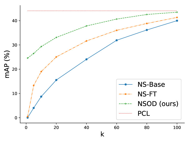
Figure 5: Detection mAP of NSOD, NS-Base, NS-FT and PCL on PASCAL VOC 2007, using different number $k$ of images per class as support set.

Method	aero	bike	bird	boat	bott	bus	car	cat	char	cow	tabl	dog	hors	mbik	prsn	plat	shep	sofa	tran	tv	mAP
NSODG	88.8	85.8	98.0	67.8	79.4	68.4	96.8	95.1	80.6	72.1	38.9	93.4	82.3	65.2	98.0	56.7	70.1	55.6	72.0	60.2	76.3
NSODX	86.4	96.9	97.1	71.4	98.5	67.1	89.9	95.1	80.0	66.8	36.5	92.9	74.2	62.9	96.9	53.1	59.9	58.8	70.1	78.9	76.7
NSOD	91.2	90.7	98.0	71.1	94.3	73.8	95.8	95.5	80.5	74.7	39.1	95.3	81.2	66.9	98.4	58.7	73.8	59.7	75.6	70.4	79.2
Method	aero	bike	bird	boat	bottle	bus	car	cat	chair	cow	table	dog	horse	mbike	persn	plant	sheep	sofa	train	tv	mAcc
NSODG	92.2	97.7	99.1	78.7	100.0	73.0	93.2	98.5	89.2	82.0	41.8	97.7	77.7	72.0	99.7	63.7	68.7	63.0	77.5	87.5	82.7
NSODX	93.1	93.4	98.2	79.2	100.0	78.9	96.3	96.7	84.0	83.5	45.1	95.7	84.2	72.9	98.5	73.3	77.2	66.1	83.3	87.7	84.3
NSOD	93.8	92.4	99.3	80.4	100.0	81.1	97.8	97.1	78.6	86.7	49.7	97.1	88.2	77.2	99.6	79.7	79.1	67.9	87.5	85.6	85.9

Table 4: Classification mAP for multi-class prediction (top) and classification mAcc for top-1 class prediction (bottom) on the trainval set of PASCAL VOC 2007. NSOD: our Nano-supervised object detection framework.

Method	aero	bike	bird	boat	bott	bus	car	cat	char	cow	tabl	dog	hors	mbik	prsn	plat	shep	sofa	tran	tv	mAP
NSODG	57.2	52.7	36.0	14.1	11.0	50.6	46.9	35.8	5.7	47.1	16.1	52.8	34.3	54.4	14.8	11.4	29.0	48.8	43.4	13.9	33.9
NSODX	58.5	51.5	37.5	11.6	10.6	55.3	48.2	40.4	5.8	49.9	16.0	51.3	31.6	56.3	14.6	9.0	34.3	45.5	42.2	20.3	34.5
NSOD	57.9	59.7	43.2	10.5	13.1	62.7	58.6	43.9	10.6	51.1	25.7	49.8	39.3	60.6	14.9	10.9	33.5	45.2	42.5	27.8	38.0
NSOD ($k=1$)	53.0	58.0	24.4	13.3	11.3	41.3	43.8	43.6	2.3	50.3	6.1	32.4	19.0	50.5	15.0	8.7	35.7	41.7	42.8	6.2	30.0
NSOD ($k=10$)	57.2	27.8	40.4	9.7	11.2	61.2	57.0	25.9	13.4	47.2	6.2	45.5	35.7	53.0	21.2	14.1	34.8	43.7	39.8	19.8	33.2
NSOD ($k=20$)	57.9	59.7	43.2	10.5	13.1	62.7	58.6	43.9	10.6	51.1	25.7	49.8	39.3	60.6	14.9	10.9	33.5	45.2	42.5	27.8	38.0

Table 5: Ablation study. Detection mAP on the test set of PASCAL VOC 2007. NSOD: our nano-supervised object detection framework.

Method	aero	bike	bird	boat	bott	bus	car	cat	char	cow	tabl	dog	hors	mbik	prsn	plat	shep	sofa	tran	tv	mAP
WSDDN [6]	65.1	58.8	58.5	33.1	39.8	68.3	60.2	59.6	34.8	64.5	30.5	43.0	56.8	82.4	25.5	41.6	61.5	55.9	65.9	63.7	53.5
OICR [8]	81.7	80.4	48.7	49.5	32.8	81.7	85.4	40.1	40.6	79.5	35.7	33.7	60.5	88.8	21.8	57.9	76.3	59.9	75.3	81.4	60.6
WSRPN [28]	77.5	81.2	55.3	19.7	44.3	80.2	86.6	69.5	10.1	87.7	68.4	52.1	84.4	91.6	57.4	63.4	77.3	58.1	57.0	53.8	63.8
PCL [1]	79.6	85.5	62.2	47.9	37.0	83.8	83.4	43.0	38.3	80.1	50.6	30.9	57.8	90.8	27.0	58.2	75.3	68.5	75.7	78.9	62.7
WS-JDS [61]	82.9	74.0	73.4	47.1	60.9	80.4	77.5	78.8	18.6	70.0	56.7	67.0	64.5	84.0	47.0	50.1	71.9	57.6	83.3	43.5	64.5
NSOD	80.0	73.3	66.1	34.0	29.0	72.6	76.5	56.4	17.7	74.7	47.5	61.4	60.5	86.4	31.9	36.6	60.8	59.1	57.4	49.1	56.6
NSOD (07+12)	78.3	78.4	70.3	34.0	34.0	75.1	76.6	66.9	24.8	76.0	45.6	69.8	67.7	88.8	34.4	41.4	67.0	62.1	67.3	40.9	60.0

Table 6: CorLoc on the trainval set of PASCAL VOC 2007. All compared methods [6, 8, 28, 1, 61] use the image-level labels in $X$; our NSOD does not.

4.3 Support set by sampling VOC 2007

As discussed in Sec. 4.1, the support set $G$ can be collected by randomly selecting $k$ images per class from the unlabeled set $X$. This is more challenging than web search, as one image may depict more than one object, as shown in Fig. 3. We randomly sample $k\in\{1,5,10,20,40,60,80,100\}$ images per class from VOC 2007 with image-level labels as $G$ and evaluate on its test set. We compare NSOD with two baselines: (1) only using $G$ to train the student $U$, denoted by NS-Base; (2) using NS-FT as described in Sec. 4.2.1.

As shown in Figure 5, NSOD yields significantly higher mAP at every $k$ compared to the baselines. In particularly, with small $k$, our improvement is substantial; with $k=80$ (around 30% of VOC 2007 training data), NSOD achieves accuracy already very close (on par) to PCL [1] (dotted horizontal line) that uses image-level labels of 100% data in VOC 2007.

4.4 Ablation Study

We conduct the ablation study on our labeling strategy, support set size, and localization on the trainval set of PASCAL VOC 2007. The support set $G$ is collected by web search.

4.4.1 Labeling strategy (classification)

Referring to subsection 3.3 in the paper, we ablate combining ${\boldsymbol{\sigma}}(S)$ and ${\boldsymbol{\sigma}}(A)$ to generate image-level pseudo-labels. ${\boldsymbol{\sigma}}(S)$ is computed based on $G$ alone, while ${\boldsymbol{\sigma}}(A)$ is computed based on the teacher model trained on $X$. We apply a hard threshold of $\frac{1}{2}$ on the predicted class probabilities of ${\boldsymbol{\sigma}}(S)$ and ${\boldsymbol{\sigma}}(A)$ to generate two sets of image-level pseudo-labels. We train two different models separately on the two sets of pseudo-labels, which we denote by NSOD_G and NSOD_X, respectively.

The classification accuracy of the two sets of pseudo-labels is first evaluated on the trainval set of VOC 2007 and shown in Table 4. It can be seen that NSOD_G and NSOD_X produce a similar classification mAP of $76.3$ vs. $76.7$, while the AP on individual classes differs. However, in terms of top-1 class accuracy, NSOD_X is better than NSOD_G. This is reasonable, as NSOD_X is fine-tuned as a $C$-way classifier, which takes the top-1 class predictions of ${\boldsymbol{\sigma}}(S)$ as pseudo-labels. The two sets of pseudo-labels are complementary by averaging ${\boldsymbol{\sigma}}(S)$ and ${\boldsymbol{\sigma}}(A)$ according to Eq.(4), denoted by NSOD. This improves both multi-class and top-1 class predictions, reaching the highest scores of $79.2$ and $85.9$, respectively.

4.4.2 Labeling strategy (detection)

To further investigate the complementary effect of the two models NSOD_G and NSOD_X, we evaluate their detection result on the test set of VOC 2007 (Table 5). The mAP of NSOD_X (34.5) is slightly greater than that of NSOD_G (33.9). Their combination (our full model NSOD) further increases mAP by $+3.5\%$ to $38.0$. The detection result on the test set is consistent with the classification result on the trainval set, which validates our idea of distilling knowledge from the support set to the unlabeled set and from the teacher to the student model.

4.4.3 Support set size

We evaluate performance for different number $k$ of web images per class of the support set $G$ in Table 5: mAP is 30.0 for $k=1$, 33.2 for $k=10$ and 38.0 for $k=20$. Further increasing $k$ presumably brings more noisy examples. How to deal with large-scale noisy web images/videos is an open problem [36, 37, 38, 39]. We keep $G$ small to avoid bringing too many noisy images, while at the same time using the unlabeled unlabeled set $X$ for more diversity.

4.4.4 Localization on the trainval set

Apart from the mAP on the test set, in Table 6 we report CorLoc on the trainval set of VOC 2007, as is common for weakly-supervised detection methods [6, 8, 28, 1, 61]. Our NSOD delivers CorLoc 56.6, which is very close to other WSOD methods despite using no annotations on $X$. Like in subsubsection 4.2.3, if we train NSOD on the union of VOC 2007 and VOC 2012 (07+12) on a large-scale, the CorLoc of NSOD (07+12) on VOC 2007 (see Table 6) is increased to 60.0, which is only 2.7% below PCL (62.7) and generally among the best-performing WSOD methods (e.g. OICR has 60.6).

5 Discussion

Our nano-supervised object detection framework basically begins with a combination of few-shot and semi-supervised classification. The former is using the few images as class prototypes [65] to estimate class probabilities per region, which are propagated at image level using the voting process of WSDDN [6]. The latter is generating pseudo-labels on the unlabeled set from these probabilities to train a classifier [20].

By using the PCL pipeline [1] and extending the unlabeled set to both VOC 2007 and VOC 2012, our NSOD achieves detection mAP very close to PCL itself trained on VOC 2007 with image-level labels. Moreover, our result is already competitive or superior to many recent WSOD solutions.

It is reasonable to expect further improvement by applying our method to very large unlabeled collections. This is facilitated by the fact that NSOD is robust to unknown classes and can discover relevant data even among non-curated collections. Moreover, since NSOD produces image-level pseudo-labels that can be used to train any weakly-supervised detection pipeline, further improvement could be expected by using these pseudo-labels with more advanced WSOD methods.

We hope that our work will inspire further research in this challenging regime of limited supervision. A challenge will be to integrate our multi-stage learning process into a single end-to-end trainable pipeline, either including the last WSOD stage (stage 4) or not.

References

- [1] P. Tang, X. Wang, S. Bai, W. Shen, X. Bai, W. Liu, A. L. Yuille, PCL: Proposal cluster learning for weakly supervised object detection, IEEE Transactions on Pattern Analysis and Machine Intelligence.
- [2] R. Girshick, Fast r-cnn, in: ICCV, 2015.
- [3] S. Ren, K. He, R. Girshick, J. Sun, Faster r-cnn: Towards real-time object detection with region proposal networks, in: NIPS, 2015.
- [4] Q. Chen, P. Wang, A. Cheng, W. Wang, Y. Zhang, J. Cheng, Robust one-stage object detection with location-aware classifiers, Pattern Recognition 105 (2020) 107334.
- [5] J. Yuan, H.-C. Xiong, Y. Xiao, W. Guan, M. Wang, R. Hong, Z.-Y. Li, Gated cnn: Integrating multi-scale feature layers for object detection, Pattern Recognition 105 (2020) 107131.
- [6] H. Bilen, A. Vedaldi, Weakly supervised deep detection networks, in: CVPR, 2016.
- [7] M. Shi, V. Ferrari, Weakly supervised object localization using size estimates, in: ECCV, 2016.
- [8] P. Tang, X. Wang, X. Bai, W. Liu, Multiple instance detection network with online instance classifier refinement, in: CVPR, 2017.
- [9] Z. Ren, Z. Yu, X. Yang, M.-Y. Liu, Y. J. Lee, A. G. Schwing, J. Kautz, Instance-aware, context-focused, and memory-efficient weakly supervised object detection, in: CVPR, 2020.
- [10] R. Gokberk Cinbis, J. Verbeek, C. Schmid, Multi-fold mil training for weakly supervised object localization, in: CVPR, 2014.
- [11] Z. Shi, P. Siva, T. Xiang, Transfer learning by ranking for weakly supervised object annotation, arXiv preprint arXiv:1705.00873.
- [12] L. Cao, F. Luo, L. Chen, Y. Sheng, H. Wang, C. Wang, R. Ji, Weakly supervised vehicle detection in satellite images via multi-instance discriminative learning, Pattern Recognition 64 (2017) 417–424.
- [13] S. Andrews, I. Tsochantaridis, T. Hofmann, Support vector machines for multiple-instance learning, in: NIPS, 2003.
- [14] Y. Tang, J. Wang, B. Gao, E. Dellandréa, R. Gaizauskas, L. Chen, Large scale semi-supervised object detection using visual and semantic knowledge transfer, in: CVPR, 2016.
- [15] J. Hoffman, D. Pathak, T. Darrell, K. Saenko, Detector discovery in the wild: Joint multiple instance and representation learning, in: CVPR, 2015.
- [16] Z. Yan, J. Liang, W. Pan, J. Li, C. Zhang, Weakly-and semi-supervised object detection with expectation-maximization algorithm, arXiv preprint arXiv:1702.08740.
- [17] S. Huang, X. Zeng, S. Wu, Z. Yu, M. Azzam, H.-S. Wong, Behavior regularized prototypical networks for semi-supervised few-shot image classification, Pattern Recognition 112 (2021) 107765.
- [18] O. Chapelle, B. Schölkopf, A. Zien, Semi-Supervised Learning, MIT Press, 2006.
- [19] J. Weston, F. Ratle, R. Collobert, Deep learning via semi-supervised embedding, in: ICML, 2008, pp. 1168–1175.
- [20] D.-H. Lee, Pseudo-label: The simple and efficient semi-supervised learning method for deep neural networks, in: ICMLW, 2013.
- [21] A. Rasmus, M. Berglund, M. Honkala, H. Valpola, T. Raiko, Semi-supervised learning with ladder networks, in: NIPS, 2015.
- [22] M.-K. Choi, J. Park, J. Jung, H. Jung, J.-H. Lee, W. J. Won, W. Y. Jung, J. Kim, S. Kwon, Co-occurrence matrix analysis-based semi-supervised training for object detection, arXiv preprint arXiv:1802.06964.
- [23] I. Radosavovic, P. Dollar, R. Girshick, G. Gkioxari, K. He, Data distillation: Towards omni-supervised learning, in: CVPR, 2018.
- [24] Z. Shi, T. M. Hospedales, T. Xiang, Bayesian joint modelling for object localisation in weakly labelled images, IEEE Trans. PAMI 37 (10) (2015) 1959–1972.
- [25] S. Marvaniya, S. Bhattacharjee, V. Manickavasagam, A. Mittal, Drawing an automatic sketch of deformable objects using only a few images, in: ECCV, 2012.
- [26] D. Modolo, V. Ferrari, Learning semantic part-based models from google images, IEEE Trans. PAMI 40 (6) (2017) 1502–1509.
- [27] P. Tang, X. Wang, Z. Huang, X. Bai, W. Liu, Deep patch learning for weakly supervised object classification and discovery, Pattern recognition 71 (2017) 446–459.
- [28] P. Tang, X. Wang, A. Wang, Y. Yan, W. Liu, J. Huang, A. Yuille, Weakly supervised region proposal network and object detection, in: ECCV, 2018.
- [29] Y. Zhang, Y. Bai, M. Ding, Y. Li, B. Ghanem, Weakly-supervised object detection via mining pseudo ground truth bounding-boxes, Pattern Recognition 84 (2018) 68–81.
- [30] Z. Zeng, B. Liu, J. Fu, H. Chao, L. Zhang, Wsod2: Learning bottom-up and top-down objectness distillation for weakly-supervised object detection, in: ICCV, 2019.
- [31] J. Zhang, H. Su, W. Zou, X. Gong, Z. Zhang, F. Shen, Cadn: A weakly supervised learning-based category-aware object detection network for surface defect detection, Pattern Recognition 109 (2021) 107571.
- [32] Y. Liu, W. Chen, H. Qu, S. H. Mahmud, K. Miao, Weakly supervised image classification and pointwise localization with graph convolutional networks, Pattern Recognition 109 (2021) 107596.
- [33] M. Gao, A. Li, R. Yu, V. I. Morariu, L. S. Davis, C-wsl: Count-guided weakly supervised localization, in: ECCV, 2018.
- [34] M. Shi, H. Caesar, V. Ferrari, Weakly supervised object localization using things and stuff transfer, in: ICCV, 2017.
- [35] J. Uijlings, S. Popov, V. Ferrari, Revisiting knowledge transfer for training object class detectors, in: CVPR, 2018, pp. 1101–1110.
- [36] S. Guo, W. Huang, H. Zhang, C. Zhuang, D. Dong, M. R. Scott, D. Huang, Curriculumnet: Weakly supervised learning from large-scale web images, in: ECCV, 2018.
- [37] Q. Tao, H. Yang, J. Cai, Exploiting web images for weakly supervised object detection, IEEE Transactions on Multimedia.
- [38] K. K. Singh, Y. J. Lee, You reap what you sow: Using videos to generate high precision object proposals for weakly-supervised object detection, in: CVPR, 2019.
- [39] X. Liang, S. Liu, Y. Wei, L. Liu, L. Lin, S. Yan, Towards computational baby learning: A weakly-supervised approach for object detection, in: CVPR, 2015.
- [40] R. Sheikhpour, M. A. Sarram, S. Gharaghani, M. A. Z. Chahooki, A survey on semi-supervised feature selection methods, Pattern Recognition 64 (2017) 141–158.
- [41] H. Cevikalp, B. Benligiray, O. N. Gerek, Semi-supervised robust deep neural networks for multi-label image classification, Pattern Recognition 100 (2020) 107164.
- [42] J. Gao, J. Wang, S. Dai, L.-J. Li, R. Nevatia, Note-rcnn: Noise tolerant ensemble rcnn for semi-supervised object detection, in: ICCV, 2019, pp. 9508–9517.
- [43] E. Hoffer, N. Ailon, Semi-supervised deep learning by metric embedding, arXiv preprint arXiv:1611.01449.
- [44] S. Laine, T. Aila, Temporal ensembling for semi-supervised learning, in: ICLR, 2017.
- [45] A. Tarvainen, H. Valpola, Mean teachers are better role models: Weight-averaged consistency targets improve semi-supervised deep learning results, in: NIPS, 2017.
- [46] P. Tang, C. Ramaiah, Y. Wang, R. Xu, C. Xiong, Proposal learning for semi-supervised object detection, in: WACV, 2021, pp. 2291–2301.
- [47] X. Dong, L. Zheng, F. Ma, Y. Yang, D. Meng, Few-example object detection with model communication, IEEE Transactions on Pattern Analysis and Machine Intelligence 41 (7) (2018) 1641–1654.
- [48] T. Tuytelaars, C. H. Lampert, M. Blaschko, W. Buntine, Unsupervised object discovery: A comparison, IJCV 88 (2) (2010) 284–302.
- [49] J. Sivic, B. C. Russell, A. A. Efros, A. Zisserman, W. T. Freeman, Discovering objects and their location in images, in: ICCV, 2005.
- [50] D. Berthelot, N. Carlini, I. Goodfellow, N. Papernot, A. Oliver, C. Raffel, Mixmatch: A holistic approach to semi-supervised learning, in: NeurIPS, 2019.
- [51] Z. Zhao, M. Shi, X. Zhao, L. Li, Active crowd counting with limited supervision, in: ECCV, 2020.
- [52] Y. Liu, Z. Wang, M. Shi, S. Satoh, Q. Zhao, H. Yang, Towards unsupervised crowd counting via regression-detection bi-knowledge transfer, in: ACM MM, 2020.
- [53] A. Bendale, T. E. Boult, Towards open set deep networks, in: CVPR, 2016, pp. 1563–1572.
- [54] I. Z. Yalniz, H. Jégou, K. Chen, M. Paluri, D. Mahajan, Billion-scale semi-supervised learning for image classification, arXiv:1905.00546.
- [55] C. L. Zitnick, P. Dollár, Edge boxes: Locating object proposals from edges, in: ECCV, 2014.
- [56] G. Hinton, O. Vinyals, J. Dean, Distilling the knowledge in a neural network, arXiv preprint arXiv:1503.02531.
- [57] Y. Wei, W. Xia, M. Lin, J. Huang, B. Ni, J. Dong, Y. Zhao, S. Yan, Hcp: A flexible cnn framework for multi-label image classification, IEEE Transactions on Pattern Analysis and Machine Intelligence 38 (9) (2016) 1901–1907.
- [58] F. Zhu, H. Li, W. Ouyang, N. Yu, X. Wang, Learning spatial regularization with image-level supervisions for multi-label image classification, in: CVPR, 2017.
- [59] M. Everingham, L. Van Gool, C. K. Williams, J. Winn, A. Zisserman, The pascal visual object classes (voc) challenge, International journal of computer vision 88 (2) (2010) 303–338.
- [60] K. Simonyan, A. Zisserman, Very deep convolutional networks for large-scale image recognition, arXiv preprint arXiv:1409.1556.
- [61] Y. Shen, R. Ji, Y. Wang, Y. Wu, L. Cao, Cyclic guidance for weakly supervised joint detection and segmentation, in: CVPR, 2019.
- [62] K. He, X. Zhang, S. Ren, J. Sun, Deep residual learning for image recognition, in: CVPR, 2016.
- [63] O. Russakovsky, J. Deng, H. Su, J. Krause, S. Satheesh, S. Ma, Z. Huang, A. Karpathy, A. Khosla, M. Bernstein, Imagenet large scale visual recognition challenge, arXiv preprint arXiv:1409.0575.
- [64] X. Zhang, J. Feng, H. Xiong, Q. Tian, Zigzag learning for weakly supervised object detection, in: CVPR, 2018.
- [65] J. Snell, K. Swersky, R. Zemel, Prototypical networks for few-shot learning, in: NIPS, 2017.