On Generalized Surrogate Duality in Mixed-Integer Nonlinear Programming

Abstract

The most important ingredient for solving mixed-integer nonlinear programs (MINLPs) to global $\epsilon$-optimality with spatial branch and bound is a tight, computationally tractable relaxation. Due to both theoretical and practical considerations, relaxations of MINLPs are usually required to be convex. Nonetheless, current optimization solver can often successfully handle a moderate presence of nonconvexities, which opens the door for the use of potentially tighter nonconvex relaxations. In this work, we exploit this fact and make use of a nonconvex relaxation obtained via aggregation of constraints: a surrogate relaxation. These relaxations were actively studied for linear integer programs in the 70s and 80s, but they have been scarcely considered since. We revisit these relaxations in an MINLP setting and show the computational benefits and challenges they can have. Additionally, we study a generalization of such relaxation that allows for multiple aggregations simultaneously and present the first algorithm that is capable of computing the best set of aggregations. We propose a multitude of computational enhancements for improving its practical performance and evaluate the algorithm’s ability to generate strong dual bounds through extensive computational experiments.

1 Introduction

We consider a mixed-integer nonlinear program (MINLP) of the form

$$\min_{x\in X}\;\left\{c^{\mathsf{T}}x\mid g_{i}(x)\leq 0\text{ for all }i\in\mathcal{M}\right\},$$ (1)

where $X:=\{x\in\mathbb{R}^{n-p}\times\mathbb{Z}^{p}\mid Ax\leq b\}$ is a compact mixed-integer linear set, each $g_{i}:\mathbb{R}^{n}\to\mathbb{R}$ is a factorable continuous function [43], and $\mathcal{M}:=\{1,\ldots,m\}$ denotes the index set of nonlinear constraints. Such a problem is called nonconvex if at least one $g_{i}$ is nonconvex, and convex otherwise. Many real-world applications are inherently nonlinear, and can be formulated as a MINLP. See, e.g., [30] for an overview.

The state-of-the-art algorithm for solving nonconvex MINLPs to $\epsilon$-global optimality is spatial branch and bound, see, e.g., [32, 53, 54]. The performance of spatial branch and bound mainly depends on the tightness of the relaxations used, which are typically convex relaxations constructed from the convexification of the nonlinear and integrality constraints. These convex relaxations are refined by branching, cutting planes, and variable bound tightening, e.g., feasibility- and optimality-based bound tightening [52, 10]. As a result of the rapid progress during the last decades, current solvers can often handle a moderate presence of nonconvex constraints efficiently. This opens the door for a practical use of potentially tighter nonconvex relaxations in MINLP solvers. One example are MILP relaxations, see [69, 46, 13]. In this paper we go one step further and explore the concept of surrogate relaxations [23]. Even more aggressively, this leads to MINLP relaxations that may contain both discrete and continuous nonlinearities.

Definition 1 (Surrogate relaxation).

For a given $\lambda\in\mathbb{R}^{m}_{+}$, we call the optimization problem

$$S(\lambda):=\min_{x\in X}\;\left\{c^{\mathsf{T}}x\mid\sum_{i\in\mathcal{M}}\lambda_{i}g_{i}(x)\leq 0\right\}$$ (2)

a surrogate relaxation of (1).

Consider $\mathcal{F}\subseteq\mathbb{R}^{n}$ the feasible region of (1), and $S_{\lambda}\subseteq\mathbb{R}^{n}$ that of (2). Throughout the whole paper we assume that $\mathcal{F}$ is not empty. Clearly, $\mathcal{F}\subseteq S_{\lambda}$ holds for every $\lambda\in\mathbb{R}^{m}_{+}$, and as such (2) provides a valid lower bound of (1). Moreover, solving (2) might be computationally more convenient than solving the original problem (1), since there is only one nonconvex constraint in $S(\lambda)$. Note that one may turn $S_{\lambda}$ into a continuous relaxation of (1) by removing the integrality restrictions. However, in this work we purposely choose to retain integrality in the relaxation and compare directly to the optimal value of (1) as opposed to its continuous relaxation.

The quality of the bound provided by $S(\lambda)$ may be highly dependent on the value of $\lambda$, and therefore it is natural to consider the surrogate dual problem in order to obtain the tightest surrogate relaxation.

Definition 2 (Surrogate dual).

We call the optimization problem

$$\sup_{\lambda\in\mathbb{R}^{m}_{+}}\;S(\lambda)\\$$ (3)

the surrogate dual of (1).

The function $S$ is lower semi-continuous [29], which means that for every sequence $\{\lambda^{t}\}_{t\in\mathbb{N}}\subseteq\mathbb{R}^{m}_{+}$ with $\lim_{t\rightarrow\infty}\lambda^{t}=\lambda^{*}$, the inequality

$$S(\lambda^{*})\leq\liminf_{t\rightarrow\infty}S(\lambda^{t})$$

holds. Thus, there might be no $\lambda\in\mathbb{R}^{m}_{+}$ such that $S(\lambda)$ is equal to (3), as can be observed in Figure 1. Therefore, it is not possible to replace the supremum in (3) by a maximum.

The surrogate dual is closely related to the well-known Lagrangian dual $\max_{\lambda\in\mathbb{R}^{m}_{+}}L(\lambda)$, where

$$L(\lambda):=\min_{x\in X}\left\{c^{\mathsf{T}}x+\sum_{i\in\mathcal{M}}\lambda_{i}g_{i}(x)\right\}\text{,}$$ (4)

but always results in a bound that is at least as good as the Lagrangian one [29, 37], i.e.,

$$S(\lambda)\geq L(\lambda) \quad\text{ for all }\lambda\in\mathbb{R}^{m}_{+}.$$ (5)

Figure 1 shows the difference between $S(\lambda)$ and $L(\lambda)$ on the two-dimensional instance of Example 1. In contrast to $L:\mathbb{R}^{m}_{+}\rightarrow\mathbb{R}$, which is a continuous and concave function, $S:\mathbb{R}^{m}_{+}\rightarrow\mathbb{R}$ is only quasi-concave [29] (i.e., the set $\{\lambda\in\mathbb{R}^{m}_{+}\mid S(\lambda)\geq\alpha\}$ is convex for all $\alpha$) and in general is discontinuous. As it can be seen in Figure 1, the main difficulty in optimizing $S(\lambda)$ for nonconvex MINLPs is that the function is most of the time “flat”, meaning that it leads to nontrivial dual bounds for only a small subset of the $\lambda$-space. To the best of our knowledge, this aspect has not received much attention in the development of algorithms that solve (3) for general MINLPs.

Example 1.

Consider the following nonconvex problem

$$\min -y$$

s.t. $$2xy+x^{2}-y^{2}-x\leq 0,$$

$$-xy-0.3x^{2}-0.2y^{2}-0.5x+1.5y\leq 0,$$

$$(x,y)\in[0,1]^{2},$$

which attains its optimal value $-0.37$ at $(x^{*},y^{*})\approx(0.52,0.37)$. The surrogate dual problem reads as

$$\sup_{(\lambda_{1},\lambda_{2})\in\mathbb{R}_{+}^{2}}\left\{\begin{aligned} \min\quad&-y\\ \text{s.t.}\quad&\lambda_{1}(2xy+x^{2}-y^{2}-x)\\ &+\lambda_{2}(-xy-0.3x^{2}-0.2y^{2}-0.5x+1.5y)\leq 0\\ &(x,y)\in[0,1]^{2}\end{aligned}\right\},$$

whereas the Lagrangian dual problem is

$$\sup_{(\lambda_{1},\lambda_{2})\in\mathbb{R}_{+}^{2}}\left\{\begin{aligned} \min\quad&-y+\lambda_{1}(2xy+x^{2}-y^{2}-x)\\ &+\lambda_{2}(-xy-0.3x^{2}-0.2y^{2}-0.5x+1.5y)\\ \text{s.t.}\quad&(x,y)\in[0,1]^{2}\end{aligned}\right\}.$$

Here the optimal solution value of the surrogate dual is $S(0.56,0.44)\approx-0.38$, which is stronger than that of the Lagrangian dual $L(0.67,0.82)\approx-0.78$. Note that for this problem neither the surrogate nor the Lagrangian dual proves global optimality of $(x^{*},y^{*})$.

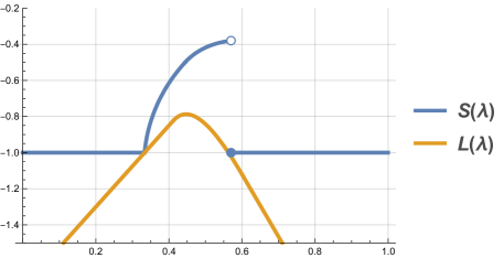
Figure 1: Plot of the surrogate and Lagrangian relaxations values for the MINLP detailed in Example 1. Note that for display purposes we plot both relaxations with respect to $\lambda_{1}$ only. Since the surrogate relaxation is invariant to scaling, we can add a normalization constraint $\left\|\lambda\right\|_{1}=\alpha$ such that $\lambda_{2}=\alpha-\lambda_{1}$ is not a free parameter any more. Additionally, we choose $\alpha$ such that $\max_{\lambda}L(\lambda)$ is attained.

Contribution.

In this paper, we revisit surrogate duality in the context of mixed-integer nonlinear programming. To the best of our knowledge, surrogate relaxations have never been considered in practice for solving general MINLPs.

The first contribution of the paper is an experimental study of a generalization of surrogate duality in the nonconvex setting that allows for multiple aggregations of the nonlinear constraints. Second, based on a row-generation method, we present the first algorithm to solve the corresponding generalized surrogate dual problem and prove its convergence. Third, we present several computational enhancements to make the algorithm practical, which includes an effective way to integrate a MINLP solver into our algorithm. Our developed algorithm shows that the quality of the generalized surrogate relaxation can be significantly stronger than that of the classic one. Finally, we provide a detailed computational analysis on publicly available benchmark instances.

Structure.

The rest of the paper is organized as follows. In Section 2, we present a literature review of surrogate duality. Section 3 discusses an algorithm from the literature for solving the classic surrogate dual problem and our new computational enhancements. In Section 4, we review a generalization of surrogate relaxations from the literature. Afterwards, in Section 5, we adapt an algorithm for the classic surrogate dual problem to the general case and prove its convergence. An exhaustive computational study using the MINLP solver SCIP on publicly available benchmark instances is given in Section 6. Afterwards, Section 7 presents ideas for future work that exploits surrogate relaxations in the tree search of spatial branch and bound. Section 8 presents concluding remarks.

2 Background

Surrogate constraints were first introduced by Glover [23] in the context of zero-one linear integer programming problems. He defined the strength of a surrogate constraint according to the dual bound achieved by it —the same notion we use in (3) and throughout our work. He also showed how to obtain the best multipliers for (3) in the case of two inequalities. Balas [7] and Geoffrion [22] extended the use of surrogate relaxations in zero-one linear programming. Their definitions of strength of a surrogate relaxation, however, differed from that of Glover. Furthermore, their notions of strength ignored integrality conditions. This allowed them to compute the best surrogate relaxation using a linear program. Later on, Glover [24] provided a unified view on the aforementioned approaches to surrogate relaxations and proposed a generalization where only a subset of constraints are used for producing an aggregation, leaving the rest explicitly enforced by the surrogate relaxation. We consider this variant via the set $X$ in (2).

A theoretical analysis of surrogate duality in a nonlinear setting was presented by Greenberg and Pierskalla [29]. They showed that finding the best multipliers amounts to optimizing a quasi-concave and in general discontinuous function and that the surrogate dual problem is at least as strong as the Lagrangian dual. They also proposed a generalization using multiple disjoint aggregation constraints. A similar generalization allowing multiple aggregations was later studied by Glover [25] along with the composite dual: a combination of surrogate and Lagrangian relaxations. These generalizations were proposed without a computational evaluation.

Regarding the link between surrogate and Lagrangian duality, Karwan and Rardin [37] presented necessary conditions for having no gap between the Lagrangian and surrogate duals. They also gave empirical evidence on why having no such gap is unlikely. As for the duality gap provided by the surrogate dual, and much like in Lagrangian duality, conditions that ensure that the surrogate dual equals the optimal solution value (e.g., constraint qualification conditions) were exhaustively studied, see [25, 51, 60] and the references therein.

The first algorithmic method for finding the optimal value of (3) is attributed to Banerjee [9]. In the context of integer linear programming, he proposed a Benders-type approach that alternates between solving a linear program (the master problem) and an integer linear program with a single constraint (the sub-problem). This approach is the one considered by us, which we describe in full detail in Section 3 adapted to the MINLP context, along with its convergence guarantees. Karwan [36] expanded on this approach, including a refinement of that of Banerjee and subgradient-based methods. Independently, Dyer [19] proposed similar methods to those of Karwan. Karwan and Rardin [37] argued in favor of Benders-based approaches for the search of multipliers, as opposed to subgradient methods, by showing that a subgradient may not provide an ascent direction for the surrogate dual. Nonetheless, a subgradient-like search procedure was proposed by Karwan and Rardin [40] with positive results in packing problems. The latter search method may also be viewed as a variant of the Benders approach of Banerjee, with the LP master problem being replaced by a computationally more efficient multiplier update. Sarin et al. [55] then proposed a different multiplier search procedure based on consecutive Lagrangian dual searches and tested it on randomly generated packing problems. Gavish and Pirkul [21] proposed a heuristic to find useful multipliers based on a sequential search over each multiplier separately while keeping the others constant. They presented computational experiments for their heuristic on packing instances as well. Kim and Kim [41] built upon the approach by Sarin et al., and developed a more efficient exact algorithm for finding the optimal multipliers. However, the guarantees of the latter hold only when the feasible set is finite.

From a different perspective, Karwan and Rardin [39] described the interplay between the branch-and-bound trees of an integer programming problem and its surrogate relaxations, to efficiently incorporate surrogate duals in branch and bound. Later on, Sarin et al. [56] showed how to integrate their Lagrangian-based multiplier search proposed in [55] into branch and bound.

From an application point of view, surrogate constraints were used in various ways. In [26], Glover presented a class of surrogate constraint primal heuristics for integer programming problems. Djerdjour et al. [18] presented a surrogate relaxation-based algorithm for knapsack problems with a quadratic objective function. Fisher et al. [20] used surrogate relaxations to construct algorithms that improve the dual and primal bounds for the job shop problem. Narciso and Lorena [48] used a surrogate relaxation approach for tackling generalized assignment problems. We refer the reader to [27, 5] for reviews on surrogate duality methods, including other applications and alternative methods for generating surrogate constraints not based on aggregations.

To the best of our knowledge, the efforts for practical implementations of multiplier search methods have mainly focused on linear integer programs. This can be explained by the maturity of the computational optimization tools available at the time most of these implementations were developed. We are only aware of two exceptions. First, the entropy approach to nonlinear programming (see [61, 68]) which uses a single aggregation-based constraint to tackle nonlinear problems, but uses an entropy-based reformulation instead of a weighted sum of the constraints. And second, the work by Nakagawa [47] who considered separable nonlinear integer programming and presented a novel algorithm for solving the surrogate dual. However, the author’s approach is tailored for a limited family of nonlinear problems. Additionally, the algorithm relies on performing, at each step, a potentially expensive enumerative procedure.

Regarding the generalization of the surrogate dual which considers multiple aggregated constraints (discussed in detail in Section 4), we are not aware of any work considering a multiplier search method with provable guarantees or a computational implementation of a heuristic approach for it. We are only aware of the discussion by Karwan and Rardin [38] regarding the searchability of multipliers for the surrogate dual generalizations proposed by Greenberg and Pierskalla [29] and Glover [25]. They argued that the lack of desirable structures (such as quasi-concavity) may impair search procedures which are directly based on the original surrogate dual. They showed, however, that simple heuristics can perform empirically well; although only for the composite dual. The target of Section 5 is to show that a Benders approach for the case of multiple aggregations can also be used. Moreover, we prove that such an approach has similar convergence guarantees to those of the single-aggregation surrogate dual.

3 Surrogate duality in MINLPs

While surrogate duality in its broader definition can be applied in theory to any MINLP, to the best of our knowledge, only mixed-integer linear programming problems have been considered for practical applications. Much less attention has been given to the general MINLP case, due to the potential nonconvexity of the resulting problems. Figure 2 illustrates the possible drawbacks and benefits of a nonconvex surrogate relaxation, namely, potentially tight relaxations and potentially convex (Figure 2), nonconvex (Figure 2 and 2) and even disconnected (Figure 2) feasible regions.

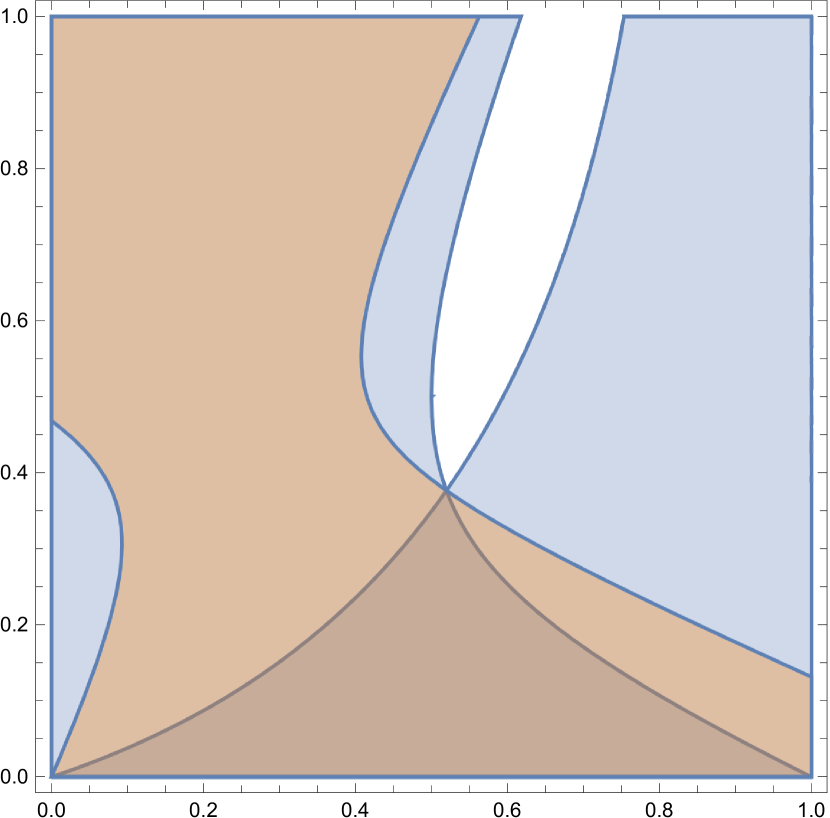
$\lambda=(\frac{3}{4},\frac{1}{4})$

(a) $S_{\lambda}$ nonconvex

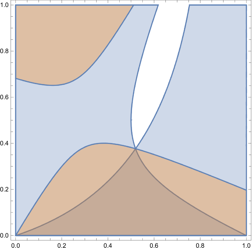
$\lambda=(\frac{2}{3},\frac{1}{3})$

(b) $S_{\lambda}$ disconnected

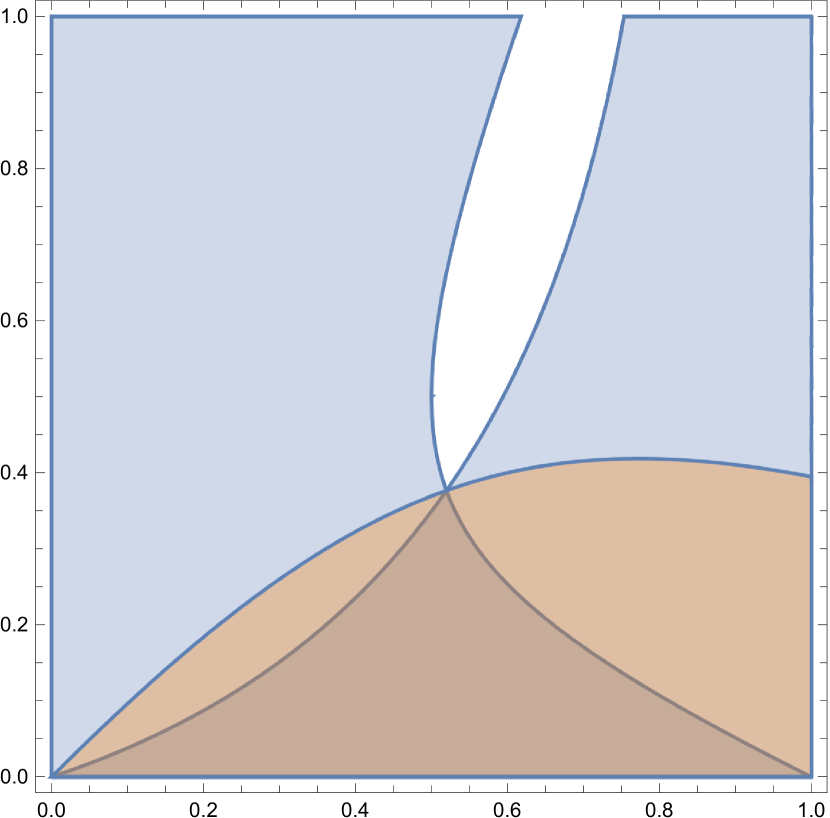
$\lambda=(\frac{1}{2},\frac{1}{2})$

(c) $S_{\lambda}$ convex

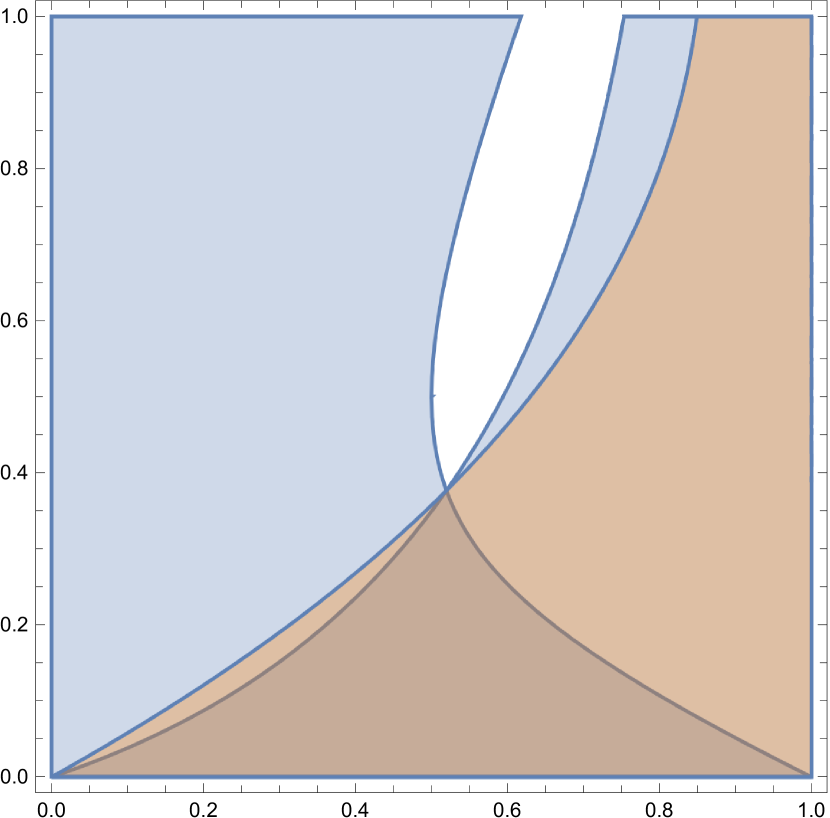
$\lambda=(\frac{1}{4},\frac{3}{4})$

(d) $S_{\lambda}$ complement of a convex set

Figure 2: Different surrogate relaxations $S_{\lambda}$ for the nonconvex optimization problem in Example 1. The feasible region defined by each nonlinear constraint is blue and the set $S_{\lambda}$ is orange. Depending on the choice of $\lambda$, $S_{\lambda}$ might be nonconvex, disconnected, convex, or reverse convex.

We investigate the trade-off between the computational effort required to solve surrogate relaxations and the quality of the resulting dual bounds. In this section, we show how to overcome the computational difficulties faced when solving the surrogate dual with a Benders-type algorithm. This type of algorithm was presented independently by Banerjee [9], Karwan [36], and Dyer [19].

As we mentioned in Section 2, other algorithms for solving the surrogate dual exist, such as subgradient-based algorithms [36, 19, 55]. However, we use the Benders-type approach because its extension to the generalized surrogate dual problem (which we discuss in Section 4) is straightforward. It is unclear whether the subgradient-based algorithms can be extended to work for the generalization, and if their convergence guarantees can be carried over.

3.1 Solving the surrogate dual via Benders

In order to solve (3) (or at least find a good $\lambda$ multiplier), we follow a known Benders-type algorithm, see [36, 19], which we review here. The Benders algorithm is an iterative approach that alternates between solving a, so-called, master- and sub-problem. The master problem searches for the next $\lambda$ aggregation and the sub-problem solves $S(\lambda)$. Note that the value of an optimal solution $\bar{x}$ of $S(\lambda)$, i.e., $c^{\mathsf{T}}\bar{x}$, is a valid dual bound for (1). To ensure that the point $\bar{x}$ is not considered in later iterations, i.e., $\bar{x}\not\in S_{\lambda}$, the Benders algorithm uses the master problem to compute a new vector $\lambda$ that ensures $\sum_{i\in\mathcal{M}}\lambda_{i}g_{i}(\bar{x})>0$. This can be done by maximizing constraint violation. More precisely, given $\mathcal{X}\subset\mathbb{R}^{n}$ the set of previously generated points of the sub-problems, the master problem reads as

$$\max \Psi$$ (6)

s.t. $$\sum_{i\in\mathcal{M}}\lambda_{i}g_{i}(\bar{x})\geq\Psi \text{ for all }\bar{x}\in\mathcal{X},$$

$$\left\|\lambda\right\|_{1}\leq 1,$$

$$\lambda\in\mathbb{R}^{m}_{+},$$

$$\Psi\in\mathbb{R}_{+}.$$

Due to the fact that each aggregation constraint is scaling invariant, it is necessary to add a normalization, e.g., $\left\|\lambda\right\|_{1}\leq 1$, to the master problem. The resulting scheme, formalized in Algorithm 1, terminates once the solution value of (6) is smaller than a fixed value $\epsilon>0$. An illustration of the algorithm for the nonconvex problem in Example 1 is given in Figure 3.

0:  MINLP of the form (1), threshold $\epsilon>0$

0:  optimal value $D\in\mathbb{R}$ of the surrogate dual

1:  initialize $\lambda\leftarrow 0\in\mathbb{R}^{m}_{+}$, $\Psi\leftarrow\infty$, $\mathcal{X}\leftarrow\emptyset$, $D\leftarrow-\infty$

2:  while $\Psi\geq\epsilon$ do

3:     $\bar{x}\leftarrow\operatorname*{argmin}_{x}\{c^{\mathsf{T}}x\mid x\in S_{\lambda}\}$

4:     $D\leftarrow\max\{D,c^{\mathsf{T}}\bar{x}\}$

5:     $\mathcal{X}\leftarrow\mathcal{X}\cup\{\bar{x}\}$

6:     $(\lambda,\Psi)\leftarrow$ optimal solution of (6) for $\mathcal{X}$

7:  end while

8:  return  $D$

Algorithm 1 Benders algorithm for the surrogate dual.

Remark 1.

Instead of finding an aggregation vector that maximizes the violation of all points in $\mathcal{X}$, Dyer [19] uses an interior point for the polytope that is given by the so far found inequalities. This can be achieved by scaling $\Psi$ in each constraint of (6) depending on the values $g_{i}(\bar{x})$ for each $i\in\mathcal{M}$. In our experiments, however, we have observed that maximizing the violation significantly improved the quality of the computed dual bounds.

Although originally proposed for linear integer programming problems, Algorithm 1 can be attributed to Banerjee [9]. Using his analysis, Karwan [36] proved the following theorem for the case of linear constraints.

Theorem 1.

Denote by $\{(\lambda^{t},\Psi^{t})\}_{t\in\mathbb{N}}$ the sequence of values obtained in Step 6 of Algorithm 1 for $\epsilon=0$. If all $g_{i}$ are linear for all $i\in\mathcal{M}$ then Algorithm 1 either

• terminates in $T$ steps, in which case $\max_{1\leq t\leq T}S(\lambda^{t})$ is equal to (3), or

• the sequence $\{S(\lambda^{t})\}_{t\in\mathbb{N}}$ has a sub-sequence converging to (3).

We prove a stronger version of this theorem in Section 5 that also works for nonlinear constraints. Note that the convergence of the algorithm only relies on the solution of an LP and a nonconvex problem $S(\lambda)$, and does not make any assumption on the nature of $S(\lambda)$.

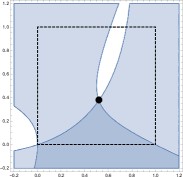
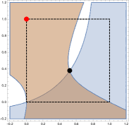
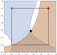
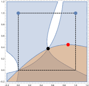
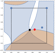
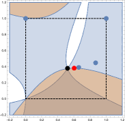
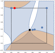
Figure 3: An illustration of the Benders algorithm for the nonconvex optimization problem of Example 1. The black point is the optimal solution to the original problem, the dashed lines correspond to the variable bounds, the light blue regions are the feasible sets of each nonlinear constraint, and the orange region is $S_{\lambda}$ for the different values of $\lambda\in\mathbb{R}_{+}^{2}$ that are computed during the Benders algorithm. The red points are the optimal solutions at each iteration and any red point becomes blue in the next iteration as part of the set $\mathcal{X}$ of points to be separated. The algorithm converges after seven iteration (from left to write in both rows of the figure), whereas the best multiplier $\lambda^{*}\approx(0.56,0.44)$ was found after five iterations.

3.2 Algorithmic enhancements

In this section, we present computational enhancements that speed up Algorithm 1 and improve the quality of the dual bound that can be achieved from (3). For the sake of completeness, we also include techniques that have been tested but did not improve the quality of the computed dual bounds significantly.

3.2.1 Refined MILP relaxation

Instead of only using the initial linear constraints $Ax\leq b$ of (1), we exploit a linear programming (LP) relaxation of (1) that is available in LP-based spatial branch and bound. This relaxation contains $Ax\leq b$ but also linear constraints that have been derived from, e.g., integrality restrictions of variables (e.g., MIR cuts [50] and Gomory cuts [28]), gradient cuts [34], RLT cuts [58], SDP cuts [59], or other valid underestimators for each $g_{i}$ with $i\in\mathcal{M}$. Using a linear relaxation $A^{\prime}x\leq b^{\prime}$ with

$$X^{\prime}:=\{x\in X\mid A^{\prime}x\leq b^{\prime}\}$$ (7)

in the definition of $S_{\lambda}$ improves the value of (3) because a relaxed version of the nonlinear constraint $g_{i}(x)\leq 0$ is captured in $S_{\lambda}$ even if $\lambda_{i}$ is zero.

Another way to further strengthen the linear relaxation is to make use of objective cutoff information that is available in spatial branch and bound. Suppose that there is a feasible, but not necessarily optimal, solution $x^{*}$ to (1). Then, the linear relaxation can be strengthened by adding the inequality $c^{\mathsf{T}}x\leq c^{\mathsf{T}}x^{*}$. Adding this inequality preserves all optimal solutions of (1) and might improve the optimal value of (3).

In our experiments, we observed that utilizing the LP relaxation that has been constructed in spatial branch and bound is the most crucial ingredient to obtain strong dual bounds with surrogate relaxations, while the objective cutoff has only a negligible impact on the quality of the computed dual bounds but helps in solving $S(\lambda)$ faster.

3.2.2 Dual objective cutoff in the sub-problem

There is an undesired phenomenon present in Algorithm 1: the sequence of dual bounds provided by $c^{\mathsf{T}}x^{*}$ in Step 3 might not be monotone, i.e., the algorithm can spend several iterations generating points that will not lead to an improvement in the dual bound $D$.

One way to overcome this problem is to add a dual objective cutoff $c^{\mathsf{T}}x\geq D$ to the sub-problem $S(\lambda)$. This enforces the sequence of dual bounds to be monotone. Adding such a constraint does not change the convergence/correctness guarantees of Algorithm 1 and it can improve the progress of the subsequent dual bounds. Moreover, such a cutoff can be used to filter the set $\mathcal{X}$ and thus reduce the size of the LP (6). Consider Figure 3 for the effect of such a cutoff: the best dual bound is found at iteration five, meaning that the two last iterations could be avoided. We also observed this behavior in other experiments, confirming the quality increase in the dual bounds provided throughout the algorithm.

The dual objective cutoff has an unfortunate drawback. Adding a constraint that is parallel to the objective function increases degeneracy. The degeneracy affects essential components of a branch-and-bound solver, e.g., pseudocost branching [11], which typically makes the problem harder to solve. In the case of the Benders algorithm, adding this cutoff significantly increases the time for solving the sub-problem, resulting in an overall negative effect on the algorithm. We confirmed this with extensive computational experiments and decided not to include this feature in our final implementation.

Fortunately, we can still carry dual information through different iterations and improve the performance of the algorithm, without having to resort to a strict objective cutoff. We discuss this next.

3.2.3 Early stopping in the sub-problem

One important ingredient to speed up Algorithm 1, proposed by Karwan [36] and Dyer [19] independently, is an early stopping criterion while solving $S(\lambda)$. In our setting, problem $S(\lambda)$ is the bottleneck of Algorithm 1. This makes any technique that can speed up the solving process of $S(\lambda)$ a crucial feature for Algorithm 1.

Assume that Algorithm 1 proved a dual bound $D$ in some previous iteration. It is possible to stop the solving process of $S(\lambda)$ if a point $\bar{x}\in S_{\lambda}$ with $c^{\mathsf{T}}\bar{x}\leq D$ has been found. The point $\bar{x}$ both provides a new inequality for (6) violated by $\lambda$ (as $\bar{x}\in S_{\lambda}$) and shows $S(\lambda)\leq D$, i.e., $\lambda$ will not lead to a better dual bound. All convergence and correctness statements regarding Theorem 1 remain valid after this modification.

Furthermore, we can apply the same idea with any choice of $D$. In this scenario, $D$ would act as a target dual bound that we want to prove. Due to the fact that the Benders-type algorithm is computationally expensive, one might require a minimum improvement in the dual bound. Empirically, we observed that solving $S(\lambda)$ to global optimality for difficult MINLPs requires a lot of time. However, finding a good quality solution for $S(\lambda)$ is usually fast. This allows us to early stop most of the sub-problems and only spend time on those sub-problems that will likely result in a dual bound that is at least as good as the target value $D$.

In our computational study presented in Section 6, we show that the early stopping technique is crucial to prove significantly better dual bounds than the best known dual bounds in the literature on difficult MINLPs.

3.3 Empirical observations

For the implementation of Algorithm 1, we use the MINLP solver SCIP

1. to construct a linear relaxation $A^{\prime}x\leq b^{\prime}$ for (1),

2. to find an objective cutoff $c^{\mathsf{T}}x\leq c^{\mathsf{T}}x^{*}$, and

3. to use it as a black box to solve each $S(\lambda)$ sub-problem.

We provide more details of our implementation and the results in Section 6, but in order to provide an overall notion of the empirical impact of this algorithm to the reader, we briefly summarize some important observations.

Our proposed algorithmic enhancements proved to be key for obtaining a practical algorithm for the surrogate dual, especially the use of a refined MILP relaxation. The achieved dual bounds by only using the initial linear relaxation in Algorithm 1 were almost always dominated by the dual bounds obtained by the refined MILP relaxation. Thus, utilizing the refined MILP relaxation seems mandatory for obtaining strong surrogate relaxations. Our computational study in Section 6 shows that our algorithmic enhancements for Algorithm 1 allows us to compute dual bounds that close on average 35.0% more gap (w.r.t. the best known primal bound) than the dual bounds obtained by the refined MILP relaxations, i.e., $S(0)$, on 469 affected instances.

While the overall impact of this “classic” surrogate duality is positive, we observed that the dual bound deteriorates with increasing number of nonlinear constraints. The reason is somewhat intuitive: aggregating a large number of nonconvex constraints into a single constraint may not capture the structure of the underlying MINLP. For this reason, we propose in the next Section to use generalized surrogate relaxations for solving MINLPs, which include multiple aggregation constraints. Even though the discussed relaxations are in general more difficult to solve, they can provide significantly better dual bounds.

4 Generalized surrogate duality

In the following, we discuss a generalization of surrogate relaxations that has been introduced by [25]. Instead of a single aggregation, it allows for $K\in\mathbb{N}$ aggregations of the nonlinear constraints of (1). The nonnegative vector

$$\lambda=(\lambda^{1},\lambda^{2},\ldots,\lambda^{K})\in\mathbb{R}^{Km}_{+}$$ (8)

encodes these $K$ aggregations

$$\sum_{i\in\mathcal{M}}\lambda^{k}_{i}g_{i}(x)\leq 0,\quad k\in\{1,\ldots,K\}$$ (9)

of the nonlinear constraints. Similar to $S_{\lambda}$, for a vector $\lambda\in\mathbb{R}^{Km}_{+}$ the feasible region of the $K$-surrogate relaxation is given by the intersection

$$S^{K}_{\lambda}:=\bigcap_{k=1}^{K}S_{\lambda^{k}},$$ (10)

where $S_{\lambda^{k}}$ is the feasible region of the surrogate relaxation $S(\lambda^{k})$ for $\lambda^{k}\in\mathbb{R}^{m}_{+}$. It clearly follows that $S^{K}_{\lambda}$ is a relaxation for (1). The best dual bound for (1) generated by a $K$-surrogate relaxation is given by

$$\sup_{\lambda\in\mathbb{R}^{Km}_{+}}S^{K}(\lambda),$$ (11)

which we call the $K$-surrogate dual. Note that scaling each $\lambda^{k}\in\mathbb{R}^{m}_{+}$ individually by a positive scalar does not affect the value of $S^{K}(\lambda)$, i.e.,

$$S^{K}(\ldots,\lambda^{k},\ldots)=S^{K}(\ldots,\alpha\lambda^{k},\ldots)$$

for any $\alpha>0$. Therefore, it is possible to impose additional normalization constraints $\left\|\lambda^{k}\right\|_{1}\leq 1$ for each $k\in\{1,\ldots,K\}$.

In [29], a related generalization was proposed, although not computationally tested. The paper considers a partition of constraints which are aggregated; equivalently, the support of sub-vectors $\lambda^{k}$ are assumed to be fixed and disjoint. Glover’s generalization [25] does not make any assumption on the structure of the $\lambda^{k}$ sub-vectors. As we will see, this makes a significant difference for two reasons: (a) selecting the “best” partition of constraints a-priori is a challenging task and (b) restricting the support of sub-vectors $\lambda^{k}$ to be disjoint can weaken the bound given by (11). The reason is that the optimal $\lambda$ multipliers might have to use the same constraints in multiple aggregations.

The function $S^{K}$ remains lower semi-continuous for any choice of $K$. The idea of the proof of the following proposition is similar to the one given by Glover [25] for the case of $K=1$.

Proposition 1.

If $g_{i}$ is continuous for every $i\in\mathcal{M}$ and $X$ is compact then $S^{K}:\mathbb{R}^{Km}_{+}\rightarrow\mathbb{R}$ is lower semi-continuous for any choice of $K$.

Proof.

Let $\{\lambda_{t}\}_{t\in\mathbb{N}}\subseteq\mathbb{R}^{Km}_{+}$ a sequence that converges to $\lambda^{*}$ and denote with $x^{t}\in X$ an optimal solution of $S^{K}(\lambda^{t})$. We need to show that $S^{K}(\lambda^{*})\leq\liminf_{t\to\infty}S^{K}(\lambda^{t})$. By definition, there exists a subsequence $\{\lambda^{\tau}\}_{\tau\in\mathbb{N}}$ of $\{\lambda^{t}\}_{t\in\mathbb{N}}$ such that $S^{K}(\lambda^{\tau})\to\liminf_{t\to\infty}S^{K}(\lambda^{t})$. Since $X$ is compact, there exists a subsequence $\{x^{l}\}_{l\in\mathbb{N}}$ of $\{x^{\tau}\}_{\tau\in\mathbb{N}}$ such that $\lim_{l\rightarrow\infty}x^{l}=x^{*}$. As $\{\lambda^{l}\}_{l\in\mathbb{N}}$ is a subsequence of $\{\lambda^{\tau}\}_{\tau\in\mathbb{N}}$, we have that $\lim_{l\rightarrow\infty}S^{K}(\lambda^{l})=\liminf_{t\to\infty}S^{K}(\lambda^{t})$. From $x^{l}\in S^{K}_{\lambda^{l}}$ it follows that

$$\sum_{i\in\mathcal{M}}\lambda_{km+i}^{l}\,g_{i}(x^{l})\leq 0$$

for every $k\in\{1,\ldots,K\}$, which is equivalent to

$$\max_{1\leq k\leq K}\sum_{i\in\mathcal{M}}\lambda_{km+i}^{l}\,g_{i}(x^{l})\leq 0\,.$$

Because the $g_{i}$ are continuous and the maximum of continuous functions is still continuous, it follows that

$$\max_{1\leq k\leq K}\sum_{i\in\mathcal{M}}\lambda_{km+i}^{*}\,g_{i}(x^{*})=\lim_{l\rightarrow\infty}\max_{1\leq k\leq K}\sum_{i\in\mathcal{M}}\lambda_{km+i}^{l}\,g_{i}(x^{l})\leq 0.$$

Hence, $x^{*}$ is feasible but not necessarily optimal for $S^{K}(\lambda^{*})$. Therefore,

$$S^{K}(\lambda^{*})\leq c^{\mathsf{T}}x^{*}=\lim_{l\rightarrow\infty}c^{\mathsf{T}}x^{l}=\lim_{l\rightarrow\infty}S^{K}(\lambda^{l})=\liminf_{t\rightarrow\infty}S^{K}(\lambda^{t})\,.$$

∎

One important difference to the classic surrogate dual is that $S^{K}(\lambda)$ is no longer quasi-concave. The following example shows this even for the case of $K=2$ and two linear constraints.

Example 2.

Let $K=2$ and consider the linear program

$$\min y$$

s.t. $$4x-8y+3.2\leq 0,$$

$$5x-y-1.5\leq 0,$$

$$(x,y)\in[0,1]^{2},$$

which contains two variables and two linear constraints. Due to the symmetry of the generalized surrogate dual, $S^{2}(\lambda)=S^{2}(\mu)\approx 0.30$ holds for the aggregation vectors $\lambda:=((0.7,0.3),(0.3,0.7))$ and $\mu:=((0.3,0.7),(0.7,0.3))$. However, using the convex combination $\lambda/2+\mu/2$ we have that $S^{2}(\lambda/2+\mu/2)\approx 0.19$, which is smaller than $S^{2}(\lambda)$ and $S^{2}(\mu)$ and thereby shows that $S^{2}$ is not quasi-concave. See Figure 4 for an illustration of the counterexample.

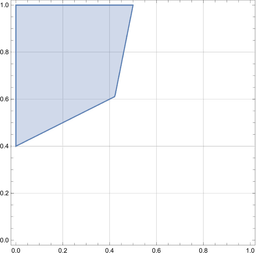
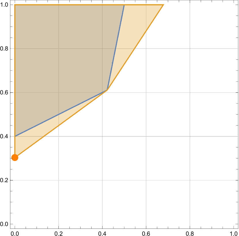
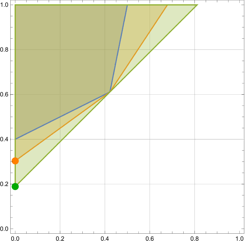
Figure 4: A visualization of Example 2 that shows that $S^{K}$ is in general not quasi-concave for $K>1$. The blue region is the feasible set defined by two original inequalities. The orange region depicts both $S^{2}_{\lambda}$ and $S^{2}_{\mu}$, while the green region is their convex combination $S^{2}_{(\lambda+\mu)/2}$. The example shows $S^{2}(\lambda)=S^{2}(\mu)>S^{2}((\lambda+\mu)/2)$, which proves that $S^{2}$ is not quasi-concave.

Due to the fact $S^{K}$ is in general not quasi-concave, gradient descent-based algorithms for optimizing (3), as in [36], do not solve (11) to global optimality. Even though (11) is substantially more difficult to solve than (3), the following theorem shows that it might be beneficial to consider larger $K$ to obtain tight relaxations for (1).

Theorem 2.

The inequality

$$\sup_{\lambda\in\mathbb{R}^{Km}_{+}}S^{K}(\lambda)\leq\sup_{\lambda\in\mathbb{R}^{(K+1)m}_{+}}S^{K+1}(\lambda)$$ (12)

holds for any $K\in\mathbb{N}$. Furthermore, $\sup_{\lambda\in\mathbb{R}^{m^{2}}_{+}}S^{m}(\lambda)$ is equal to the optimal solution value of (1).

Proof.

Note that $S^{K}(\lambda)=S^{K+1}(\lambda,0)$ holds for any $\lambda\in\mathbb{R}^{Km}_{+}$. The result follows from

$$\sup_{\lambda\in\mathbb{R}^{Km}_{+}}S^{K+1}(\lambda,0)\leq\sup_{\lambda\in\mathbb{R}^{(K+1)m}_{+}}S^{K+1}(\lambda)\ .$$

To prove the second part it is enough to see that the aggregation constraints for

$$\lambda=(e_{1},e_{2},\ldots,e_{m})\in\mathbb{R}^{m^{2}}_{+},$$

with $e_{i}$ being the $i$-th $m$-dimensional unit vector, are equal to the constraints of (1). ∎

Theorem 2 shows the potential of generalized surrogate duality. Using a large enough $K$ implies that the value of (11) is equal to the optimal value of the MINLP. The following example shows that going from $K=1$ to $K=2$ can have a tremendous impact on the quality of the surrogate relaxation:

Example 3.

Consider the following NLP with four nonlinear constraints and four unbounded variables:

$$\min\quad -x-y$$

s.t. $$x^{3}-z\leq 0$$

$$x^{3}+z\leq 0$$

$$y^{3}+w\leq 0$$

$$y^{3}-w\leq 0$$

$$(x,y,z,w)\in\mathbb{R}^{4}$$

It is easy to see that $(0,0,0,0)$ is the optimal solution. First, note that the classic surrogate dual, i.e., when only a single aggregation is allowed, is unbounded. For an aggregation $\lambda\in\mathbb{R}^{4}$, the sole constraint in the corresponding surrogate relaxation is

$$(\lambda_{1}+\lambda_{2})x^{3}+(-\lambda_{1}+\lambda_{2})z+(\lambda_{3}+\lambda_{4})y^{3}+(\lambda_{3}-\lambda_{4})w\leq 0.$$

If either $\lambda_{1}\neq\lambda_{2}$ or $\lambda_{3}\neq\lambda_{4}$, then the relaxation is clearly unbounded, as $z$ and $w$ are free variables. If $\lambda_{1}=\lambda_{2}$ and $\lambda_{3}=\lambda_{4}$, the aggregation reads $2\lambda_{1}x^{3}+2\lambda_{3}y^{3}\leq 0$, which also yields an unbounded surrogate relaxation.

Consider the two aggregation vectors $\lambda=(\lambda^{1},\lambda^{2})$ with $\lambda^{1}=(1/2,1/2,0,0)$ and $\lambda^{2}=(0,0,1/2,1/2)$. Using the $2$-surrogate relaxation obtained from $\lambda$ immediately implies tighter variable bounds $x\leq 0$ and $y\leq 0$, which proves optimality of $(0,0,0,0)$.

5 An algorithm for the $K$-surrogate dual

Even though (11) yields a strong relaxation for sufficiently large $K$, it is computationally more challenging to solve than (3). To the best of our knowledge, there is no algorithm in the literature known that can solve (11). Due to the missing quasi-concavity property of $S^{K}$, it is not possible to adjust each of the $K$ aggregation vectors independently and thus an alternating-type method based on the $K=1$ case could provide weak bounds.

In this section, we present the first algorithm for solving (11). The idea of the algorithm is the same as before: a master problem will generate an aggregation vector $(\lambda^{1},\ldots,\lambda^{K})$ and the sub-problem will solve the $K$-surrogate relaxation corresponding to $(\lambda^{1},\ldots,\lambda^{K})$. The only differences to Algorithm 1 are that we replace the LP master problem by a MILP master problem and solve $S^{K}(\lambda^{1},\ldots,\lambda^{K})$ instead of $S(\lambda)$.

Generalizing the Benders-type algorithm.

Assume that we have found a solution $\bar{x}$ after solving $S^{K}(\lambda^{1},\ldots,\lambda^{K})$. In the next iteration, we need to make sure that the point $\bar{x}$ is infeasible for at least one of the aggregated constraints. This can be written as a disjunctive constraint

$$\bigvee_{k=1}^{K}\left(\sum_{i\in\mathcal{M}}\lambda^{k}_{i}g_{i}(\bar{x})>0\right)$$ (13)

that contains $K$ many inequalities. As in (6), we replace the strict inequality by maximizing the activity of $\sum_{i\in\mathcal{M}}\lambda^{k}_{i}g_{i}(\bar{x})$ for all $k\in\{1,\ldots,K\}$. The master problem for the generalized Benders algorithm then reads as

$$\max \Psi$$ (14)

s.t. $$\bigvee_{k=1}^{K}\left(\sum_{i\in\mathcal{M}}\lambda^{k}_{i}g_{i}(\bar{x})\geq\Psi\right) \text{ for all }\bar{x}\in\mathcal{X},$$

$$\left\|\lambda^{k}\right\|_{1}\leq 1,\,\lambda^{k}\in\mathbb{R}_{+}^{m} \text{ for all }k\in\{1,\ldots,K\},$$

where $\mathcal{X}\subseteq X$ is the set of generated points of the sub-problems. One way to exactly solve (14) is to enumerate and solve all possible LPs that are being encoded by the disjunctions. Each LP is constructed by choosing exactly one of the linear constraints of each disjunction. However, following this approach is clearly prohibitively expensive because there are $K^{|\mathcal{X}|}$ many LPs.

Instead, we present an equivalent MILP formulation that enables us to solve (14) more efficiently by exploiting heuristics and symmetry breaking techniques that have been exclusively developed for MILPs.

Solving the master problem.

Modeling the master problem with a, so-called, big-M formulation solves orders of magnitudes faster. An equivalent MILP formulation of (14) reads as

$$\max \Psi$$ (15)

s.t. $$\sum_{i\in\mathcal{M}}\lambda^{k}_{i}g_{i}(\bar{x})\geq\Psi-M(1-z_{k}^{\bar{x}}) \text{ for all }k\in\{1,\ldots,K\},\,\bar{x}\in\mathcal{X},$$

$$\sum_{k=1}^{K}z_{k}^{\bar{x}}=1 \text{ for all }\bar{x}\in\mathcal{X},$$

$$z_{k}^{\bar{x}}\in\{0,1\} \text{ for all }k\in\{1,\ldots,K\},\,\bar{x}\in\mathcal{X},$$

$$\left\|\lambda^{k}\right\|_{1}\leq 1,\,\lambda^{k}\in\mathbb{R}_{+}^{m} \text{ for all }k\in\{1,\ldots,K\},$$

where $M$ is a large constant. A binary variable $z_{k}^{\bar{x}}$ indicates if the $k$-th disjunction of (14) is used to cut off the point $\bar{x}\in\mathcal{X}$. Due to the normalization $\left\|\lambda^{k}\right\|_{1}\leq 1$, it is possible to bound $M$ by $\max_{i\in\mathcal{M}}|g_{i}(\bar{x})|$. Even more, since the optimal $\Psi$ values of (15) are non-increasing, we could use the optimal $\Psi_{prev}$ of the previous iteration as a bound on $M$. Thus, it is possible to bound $M$ by $\min\{\max_{i\in\mathcal{M}}|g_{i}(\bar{x})|,\Psi_{prev}\}$.

Remark 2.

Big-M formulations are typically not considered strong in MILPs, given their usual weak LP relaxations. Other formulations in extended spaces can yield better theoretical guarantees when solving problems like (15), see, e.g., [8], [63], and [12]. The drawback of these extended formulations is that they require to add copies of the $\lambda$ variables depending on the number of disjunctions. In [62], the author proposes an alternative that does not create variable copies, but that can be costly to construct unless special structure is present. In our case, however, as we will discuss in Section 5.3, we do not require a tight LP relaxation of (14) and thus we opted to use (15).

The whole algorithm for the $K$-surrogate dual problem is stated in Algorithm 2. Even though (15) is more difficult to solve than (6), the following example shows that Algorithm 2 can compute significantly better dual bounds than Algorithm 1.

0:  MINLP of the form (1), threshold $\epsilon>0$, $K\in\mathbb{N}$ aggregations

0:  optimal value $D\in\mathbb{R}$ of the $K$-surrogate dual

1:  initialize $\lambda\leftarrow 0\in\mathbb{R}^{Km}_{+}$, $\Psi\leftarrow\infty$, $\mathcal{X}\leftarrow\emptyset$, $D\leftarrow-\infty$

2:  while $\Psi\geq\epsilon$ do

3:     $\bar{x}\leftarrow\operatorname*{argmin}_{x}\{c^{\mathsf{T}}x\mid x\in S^{K}_{\lambda}\}$

4:     $D\leftarrow\max\{D,c^{\mathsf{T}}\bar{x}\}$

5:     $\mathcal{X}\leftarrow\mathcal{X}\cup\{\bar{x}\}$

6:     $(\lambda,\Psi)\leftarrow$ optimal solution of (14) for $\mathcal{X}$

7:  end while

8:  return  $D$

Algorithm 2 Benders algorithm for the $K$-surrogate dual.

Example 4.

We briefly discuss the results of Algorithm 2 for the instance genpooling_lee1 from the MINLPLib. The instance consists of 20 nonlinear, 59 linear constraints, 9 binary, and 40 continuous variables after preprocessing. The classic surrogate dual, i.e., $K=1$, could be solved to optimality, whereas for $K=2$ and $K=3$ the algorithm hit the iteration limit. Nevertheless, the dual bound $-5064.2$ achieved for $K=2$ and the dual bound $-4973.2$ for $K=3$ are significantly better than the dual bound of $-5246.0$ for $K=1$, see Figure 5.

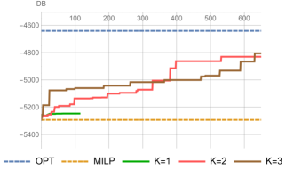
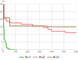
Figure 5: Results of Algorithm 2 for the instance genpooling_lee1 for different choices of $K$. The first plot shows the progress of the proved dual bound and the second plot the value of $\Psi$ for the first $600$ iterations. The blue line is the optimal solution value of the MINLP and the yellow line that of the MILP relaxation.

5.1 Convergence

In the following, we show that the dual bounds obtained by Algorithm 2 converges to the optimal value of the $K$-surrogate dual. The idea of the proof is similar to the one presented by [40] for the case of $K=1$ and linear constraints.

Theorem 3.

Denote by $\{(\lambda^{t},\Psi^{t})\}_{t\in\mathbb{N}}$ the sequence of values obtained after solving (14) in Algorithm 2 for $\epsilon=0$. The algorithm either

• terminates in $T$ steps, i.e., $\Psi^{T}=0$, in which case $\max_{1\leq t\leq T}S^{K}(\lambda^{t})$ is equal to (11), or

• $\sup_{t\geq 1}S^{K}(\lambda^{t})$ is equal to (11).

Proof.

Let $OPT$ be the optimal value of (11) and let $x^{t}\in X$ be an optimal solution obtained from solving $S^{K}(\lambda^{t})$ at iteration $t$.

• If the algorithm terminates after $T$ iterations, i.e., $\Psi^{T}=0$, then there is at least one point $x^{1},\ldots,x^{T}$ that is feasible for $S^{K}(\lambda)$ for any choice $\lambda\in\mathbb{R}^{Km}$. This implies $OPT=\max_{1\leq t\leq T}\{c^{\mathsf{T}}x^{t}\}$.

• Now assume that the algorithm does not converge in a finite number of steps, i.e., $\Psi^{t}>0$ for all $t\geq 1$. Then, there are converging subsequences

  • $\{\Psi^{l}\}_{l\in\mathbb{N}}\subseteq\{\Psi^{t}\}_{t\in\mathbb{N}}$ such that $\lim_{l\rightarrow\infty}\Psi^{l}=\Psi^{*}\geq 0$ because $\Psi^{t}\geq\Psi^{t+1}$ and $\Psi^{t}\geq 0$ hold for all $t$,

  • $\{\lambda^{l}\}_{l\in\mathbb{N}}\subseteq\{\lambda^{t}\}_{t\in\mathbb{N}}$ such that $\lim_{l\rightarrow\infty}\lambda^{l}=\lambda^{*}$ because $\left\|\lambda^{t}\right\|_{1}\leq 1$, and

  • $\{x^{l}\}_{l\in\mathbb{N}}\subseteq\{x^{t}\}_{t\in\mathbb{N}}$ such that $\lim_{l\rightarrow\infty}x^{l}=x^{*}$ because $\{x^{t}\}\subseteq X$, which is assumed to be compact.

  First, we show $\Psi^{*}=0$. Note that $x^{l}$ is an optimal solution to $S^{K}(\lambda^{l})$. This means that $x^{l}$ satisfies all aggregation constraints, i.e., $\sum_{i\in\mathcal{M}}\lambda_{km+i}^{l}\,g_{i}(x^{l})\leq 0$ for all $k=1,\ldots,K$, which is equivalent to the inequality $\max_{1\leq k\leq K}\sum_{i\in\mathcal{M}}\lambda_{km+i}^{l}\,g_{i}(x^{l})\leq 0$. After solving (14), we know that $\Psi^{l}$ is equal to the minimum violation of the disjunction constraints for the points $x^{1},\ldots,x^{l-1}$. This implies the inequality

  $$\Psi^{l}=\min_{1\leq t\leq l-1}\max_{1\leq k\leq K}\sum_{i\in\mathcal{M}}\lambda_{km+i}^{l}\,g_{i}(x^{t})\leq\max_{1\leq k\leq K}\sum_{i\in\mathcal{M}}\lambda_{km+i}^{l}\,g_{i}(x^{l-1}),$$

  which uses the fact that the minimum over all points $x^{1},\ldots,x^{l-1}$ is bounded by the value for $x^{l-1}$. Both inequalities combined show that

  $$\max_{1\leq k\leq K}\sum_{i\in\mathcal{M}}\lambda_{km+i}^{l}\,g_{i}(x^{l})\leq 0<\psi^{l}\leq\max_{1\leq k\leq K}\sum_{i\in\mathcal{M}}\lambda_{km+i}^{l}\,g_{i}(x^{l-1})$$

  for all $l\geq 0$. Using the continuity of $g_{i}$ and the fact that the maximum of finitely many continuous functions is continuous, we obtain

  $$\max_{1\leq k\leq K}\sum_{i\in\mathcal{M}}\lambda_{km+i}^{*}\,g_{i}(x^{*})\leq 0<\psi^{*}\leq\max_{1\leq k\leq K}\sum_{i\in\mathcal{M}}\lambda_{km+i}^{*}\,g_{i}(x^{*})\,$$

  which shows $\Psi^{*}=0$.

  Next, we show that $\sup_{t\geq 1}S^{K}(\lambda^{t})=OPT$. Clearly, $\sup_{t\geq 1}S^{K}(\lambda^{t})\leq OPT$. Let us now prove that $\sup_{t\geq 1}S^{K}(\lambda^{t})\geq OPT$.

  Take any $\epsilon>0$ and let $\bar{\lambda}$ be such that $S^{K}(\bar{\lambda})\geq OPT-\epsilon$ and $\|\bar{\lambda}^{k}\|\leq 1$ for all $k\in\{1,\ldots,K\}$. By definition,

  $$\Psi^{l}\geq\min_{1\leq t\leq l-1}\max_{1\leq k\leq K}\sum_{i\in\mathcal{M}}\bar{\lambda}_{km+i}\,g_{i}(x^{t}).$$

  Computing the limit when $l$ goes to infinity, we obtain

  $$0\geq\inf_{1\leq t}\max_{1\leq k\leq K}\sum_{i\in\mathcal{M}}\bar{\lambda}_{km+i}\,g_{i}(x^{t}).$$

  Let $\bar{x}$ be $x^{t_{0}}$ if the infimum is achieved at $t_{0}$ or $x^{*}$ if the infimum is not achieved. Notice that

  $$\max_{1\leq k\leq K}\sum_{i\in\mathcal{M}}\bar{\lambda}_{km+i}\,g_{i}(\bar{x})\leq 0.$$

  This last inequality implies that $\bar{x}$ is feasible for $S^{K}(\bar{\lambda})$. Hence,

  $$OPT-\epsilon\leq S^{K}(\bar{\lambda})\leq c^{\mathsf{T}}\bar{x}\leq\sup_{t\geq 1}S^{K}(\lambda^{t}).$$

  Since $\epsilon>0$ is arbitrary, we conclude that $\sup_{t\geq 1}S^{K}(\lambda^{t})\geq OPT$.

∎

The proof of Theorem 3 shows that $\{\Psi^{t}\}_{t\in\mathbb{N}}$ always converge to zero. A direct consequence of this fact is that the Algorithm 2 converges in finite steps for any $\epsilon>0$.

We now discuss computational enhancements meant for improving the performance of the proposed algorithm to solve the $K$-surrogate dual. As in the case $K=1$, we also report techniques that we did not include in our final implementation.

5.2 Multiplier symmetry breaking

One difficulty of optimizing the $K$-surrogate dual is that (14) and (15) might contain many equivalent solutions. For example, any permutation $\pi$ of the set $\{1,\ldots,K\}$ implies that the sub-problem $S^{K}(\lambda)$ with $\lambda=(\lambda^{1},\ldots,\lambda^{K})$ is equivalent to $S^{K}(\lambda^{\pi})$ with $\lambda^{\pi}=(\lambda^{\pi_{1}},\ldots,\lambda^{\pi_{K}})$. This symmetry slows down Algorithm 2, as it heavily impacts the solution time of the master problem. We refer to [42] for an overview of symmetry in integer programming.

One way to overcome the problem of equivalent solutions is to explicitly break symmetry in the $\lambda^{1},\ldots,\lambda^{K}$ vectors. One way is to add the constraints

$$\lambda^{1}\succeq_{\text{lex}}\lambda^{2}\succeq_{\text{lex}}\ldots\succeq_{\text{lex}}\lambda^{K}$$ (16)

that enforce a lexicographical order on $\lambda^{1},\ldots,\lambda^{K}$ in (15).

Enforcing a lexicographical order $\lambda^{1}\succeq_{\text{lex}}\lambda^{2}$ on continuous vectors $\lambda^{1}$ and $\lambda^{2}$ can be modeled using the following constraints

$$\lambda^{1}_{1}\geq\lambda^{2}_{1}\text{,}$$ (17)

$$\left(\lambda^{1}_{1}=\lambda^{2}_{1}\right)\;\Rightarrow \lambda^{1}_{2}\geq\lambda^{2}_{2}\text{,}$$

$$\left(\lambda^{1}_{1}=\lambda^{2}_{1}\land\lambda^{1}_{2}=\lambda^{2}_{2}\right)\;\Rightarrow \lambda^{1}_{3}\geq\lambda^{2}_{3}\text{,}$$

$$\ldots$$

which can be reformulated linearly with additional binary variables and big-M constraints. However, we observed that adding (17) increases the complexity of (15) so much that it is not possible anymore to solve it in a reasonable amount of time. For this reason, we use only simple linear inequalities to partially break symmetry in the master problem. We propose two alternative ways. First, the constraints

$$\lambda^{1}_{1}\geq\lambda^{2}_{1}\geq\ldots\geq\lambda^{K}_{1}$$ (18)

enforce that $\lambda^{1},\ldots,\lambda^{K}$ are sorted with respect to the first component, i.e., the first nonlinear constraint. The drawback of this sorting is that if $\lambda^{k}_{1}=0$ for all $k\in\{1,\ldots,K\}$, i.e., if all aggregations in a given iteration ignore the first constraint, then (18) does not break any of the symmetry of (15).

Our second idea for breaking symmetry is to use

$$\lambda^{1}_{1} \geq\lambda^{k}_{1} \text{ for all }k\in\{2,\ldots,K\},$$ (19)

$$\lambda^{2}_{2} \geq\lambda^{k}_{2} \text{ for all }k\in\{3,\ldots,K\},$$

$$\ldots$$

$$\lambda^{K-1}_{K-1} \geq\lambda^{K}_{K-1},$$

which has a natural interpretation if the vectors $\lambda^{1},\ldots,\lambda^{K}$ are written as columns of a matrix $\Lambda\subseteq\mathbb{R}_{+}^{m\times K}$. The constraints (19) enforce that the diagonal entries $\Lambda_{k,k}$ are not smaller than $\Lambda_{k,k^{\prime}}$ for any $k^{\prime}>k$.

In our experiments, we used the Benders algorithm for $K\in\{1,2,3\}$. We observed that for these small choices of $K$, slightly better dual bounds could be computed when using (18) instead of (19). Furthermore, we also observed that both symmetry breaking inequalities had only an impact on the obtained dual bounds if the first nonlinear constraint was used in the best found solution of the Benders algorithm.

5.3 Early stopping of the master problem

Solving (15) to optimality in every iteration of the Benders algorithm is computationally expensive for $K\geq 2$. On the one hand, the true optimal value of $\Psi$ is needed to decide whether the algorithm terminated, i.e., $\Psi\leq\epsilon$. On the other hand, to ensure progress of the Benders algorithm it is enough to only compute a feasible point $(\Psi,\lambda^{1},\ldots,\lambda^{K})$ of (15) with $\Psi>0$. We balance these two opposing forces with the following early stopping method.

Given that (15) is a MILP, we use branch and bound to solve it. During the tree search of this algorithm, we have access to both a valid dual bound $\Psi_{d}$ and primal bound $\Psi_{p}$ such that the optimal $\Psi$ is contained in $[\Psi_{p},\Psi_{d}]$. Note that the primal bound can be assumed to be nonnegative as the vector of zeros is always feasible for (15). Furthermore, let $\Psi^{t}_{d}$ and $\Psi^{t}_{p}$ be the primal and dual bounds obtained from the master problem in iteration $t$ of the Benders algorithm. We stop the master problem in iteration $t+1$ as soon as $\Psi^{t+1}_{p}\geq\alpha\Psi^{t}_{d}$ holds for a fixed $\alpha\in(0,1]$. The parameter $\alpha$ controls the trade-off between proving a good dual bound $\Psi^{t+1}_{d}$ and saving time for solving the master problem. On the one hand, $\alpha=1$ implies

$$\Psi^{t+1}_{p}\geq\alpha\Psi^{t}_{d}\geq\alpha\Psi^{t+1}_{d}=\Psi^{t+1}_{d},$$

which can only be true if $\Psi^{t+1}_{p}=\Psi^{t+1}_{d}$ holds. This equality proves optimality of the master problem in iteration $t+1$. On the other hand, setting $\alpha$ close to zero means that we would stop as soon as a feasible solution to the master problem has been found. In our experiments, we observed that setting $\alpha$ to $0.2$ performs well.

5.4 Constraint filtering

Even though it is not necessary to solve the master problem in every iteration to global optimality, its complexity grows exponentially since a disjunction constraint of the form (13) is added in every iteration of the algorithm. One way to alleviate this problem is to reduce the set of nonlinear constraints to only those that are needed for a good quality solution of (11). This set of constraints is unknown in advance and challenging to compute because of the nonconvexity of the MINLP.

We tested different filtering heuristics to preselect nonlinear constraints. We used the violation of the constraints with respect to the LP, MILP, and convex NLP relaxation of the MINLP, as measures of “importance” of nonlinear constraints. We also used the connectivity of nonlinear constraints in the variable-constraint graph for discarding some constraints. Unfortunately, we could not identify a good filtering rule that selects few nonlinear constraints and results in strong bounds for (11).

However, we developed a way of capturing the idea of reducing the number of constraints considered in the master problem without having to impose such a strong a-priori filter on the constraints: an adaptive filtering, which we call support stabilization. This allows to improve the performance of the master problem without compromising the quality of the generated dual bounds. We specify this next.

5.5 Support stabilization

Direct implementations of Benders-based algorithms, much like column generation approaches, are known to suffer from convergence issues. Deriving “stabilization” techniques that can avoid oscillations of the $\lambda$ variables and tailing-off effects, among others, are a common goal for improving performance, see, e.g., [44], [6], and [4].

In the following, we present a support stabilization technique to address the exponential increase in complexity of the master problem (15) and to prevent the oscillations of the $\lambda$ variables. Since restricting the support on the aggregation vectors allows us to solve the master problem orders of magnitudes faster, we use the following strategy: once the Benders algorithm finds a multiplier vector that improves the overall dual bound, we restrict the support to that of the improving dual multiplier. This restricts the search space and improves solution times. Once stalling is detected (which corresponds to finding a local optimum of (11)), we remove the support restriction until another multiplier vector that improves the dual bound is found.

This technique enables us to solve the master problem substantially faster and, at the same time, compute better bounds on (11) in fewer iterations due to its stabilization interpretation.

5.6 Trust-region stabilization

In the previous section, we presented a form of stabilization for our algorithm, meant for both alleviating some of the computational burden when solving the master problem and preventing the support of subsequent variables to deviate. Nonetheless, the non-zero entries of the $\lambda$ vectors can (and do, in practice) vary significantly from iteration to iteration. To remedy this, we incorporated a classic stabilization technique: a box trust-region stabilization, see [17]. Given a reference solution $(\hat{\lambda}^{1},\ldots,\hat{\lambda}^{k})$, we impose the following constraint in (15)

$$\|(\lambda^{1},\ldots,\lambda^{k})-(\hat{\lambda}^{1},\ldots,\hat{\lambda}^{k})\|_{\infty}\leq\delta$$

for some parameter $\delta$. This prevents the $\lambda$ variables from oscillating excessively, and carefully updating $(\hat{\lambda}^{1},\ldots,\hat{\lambda}^{k})$ and $\delta$ can maintain the convergence guarantees of the algorithm proven in Theorem 3. In our implementation, we maintain a fixed $(\hat{\lambda}^{1},\ldots,\hat{\lambda}^{k})$ until we obtain a bound improvement or the algorithm stalls. When any of this happens, we remove the box and compute a new $(\hat{\lambda}^{1},\ldots,\hat{\lambda}^{k})$ with (15) without any stabilization added.

Remark 3.

In our experiments, we used another stabilization technique inspired by column generation’s smoothing by [66] and [49]. Let $\lambda^{best}$ be the best found primal solution so far and let $\lambda^{new}$ be the solution of the current master problem. Instead of using $\lambda^{new}$ as a new multiplier vector, we choose as next aggregation vector a convex combination between $\lambda^{best}$ and $\lambda^{new}$. This way we can control the distance between the new aggregation vector and $\lambda^{best}$. While this stabilization technique improved the performance of the Benders algorithm with respect to the algorithm with no stabilization, it performed significantly worse than the trust-region stabilization. Therefore, we did not include it in our final implementation.

6 Computational experiments

In this section, we present a computational study of the classic and generalized surrogate duality on publicly available instances of the MINLPLib [45]. We conduct three main experiments to answer the following questions:

1. ROOTGAP: How much of root gap with respect to the MILP relaxation can be closed by using the classic and $K$-surrogate dual? For how many instances could the classic and generalized Benders algorithm successfully terminate?

2. BENDERS: How much do the ideas of Section 5 improve the performance of the generalized Benders algorithm?

3. DUALBOUND: Can the generalized Benders algorithm improve on the dual bounds obtained by the MINLP solver SCIP?

Our ideas are embedded in the MINLP solver SCIP [57]. We refer to [2, 64, 65] for an overview of the general solving algorithm and MINLP features of SCIP.

6.1 Experimental setup

All three experiments use Algorithm 2 to compute a tighter dual bound in the root node. As discussed in Section 1, the quality of the surrogate relaxation strongly depends on the constructed linear relaxation of (1). Therefore, the Benders algorithm is called after the root node has been completely processed by SCIP. All generated and initial linear inequalities are added to $S_{\lambda}$.

For the ROOTGAP experiment, we run Algorithm 2 for one hour for each choice of $K\in\{1,2,3\}$. To measure how much more root gap can be closed by using $K+1$ instead of $K$, we use the best found aggregation vector of $K$ as an initial point for $K+1$. This ensures that Algorithm 2 always finds a dual bound for $K+1$ that is at least as good as the one for $K$.

In contrast to the first experiment, in the BENDERS experiment we focus on $K=3$ and do not start with an initial point for the aggregation vector. Considering only one $K$ allows us to more easily analyze the impact of each component of the Benders algorithm. We compare the following settings:

• DEFAULT: Benders algorithm applying all techniques that have been presented in Section 5.

• PLAIN: Plain version of the Benders algorithm. It uses none of the techniques of Section 5.

• NOSTAB: Same as DEFAULT but without using the trust-region of Section 5.6 and support stabilization of Section 5.5.

• NOSUPP: Same as DEFAULT but without using the support stabilization.

• NOEARLY: Same as DEFAULT but without using early termination for the master problem, described in Section 5.3.

Each of the five settings uses a time limit of one hour.

Finally, in the DUALBOUND experiment we evaluate how much the dual bounds obtained by SCIP with default settings can be improved by the Algorithm 2. First, we collect the dual bounds for all instances that could not be solved by SCIP within three hours. Afterward, we apply Algorithm 2 for $K=3$, a time limit of three hours, and set a target dual bound (see Section 3.2.3) of

$$D+(P-D)\cdot 0.2,$$

where $D$ is the dual bound obtained by default SCIP and $P$ be the best known primal bound reported in the MINLPLib. This means that we aim for a gap closed reduction of at least $20$% and early stop each sub-problem in Algorithm 2 that will provably lead to a smaller reduction.

During all three experiments, we use a gap limit of $10^{-4}$ for each sub-problem of the Benders algorithm to reduce the impact of tailing-off effects. Additionally, we chose a dual feasibility tolerance of $10^{-8}$ (SCIP’s default is $10^{-7}$) and a primal feasibility tolerance of $10^{-7}$ (SCIP’s default is $10^{-6}$).

Implementation.

We extended SCIP by a (relaxator) plug-in that solves the $K$-surrogate dual problem after the root node has been completely processed by SCIP, i.e., no more cutting planes or variable bound tightenings could be found.

The trust-region and support stabilization have been implemented as follows. Both stabilization methods are applied once an improving aggregation $\lambda^{*}$ could be found. Each entry $\lambda_{i}$ with $\lambda_{i}^{*}=0$ is fixed to zero. Otherwise, the domain of $\lambda_{i}$ is restricted to the interval

$$\left[\max\{0,\lambda_{i}^{*}-0.1\},\min\{1,\lambda_{i}^{*}+0.1\}\right].$$

Once a new improving solution has been found, we update the trust region accordingly. We remove the trust region and support stabilization in case no improving solution could be found for $20$ iterations.

Test set.

We used the publicly available instances of the MINLPLib [45], which at time of the experiments contained $1683$ instances. This includes among others instances from the first MINLPLib, the nonlinear programming library GLOBALLib, and the CMU-IBM initiative minlp.org [14]. We selected the instances that were available in OSiL format and consisted of nonlinear expressions that could be handled by SCIP, in total $1671$ instances.

Gap closed.

We use the following measure to compare dual bounds relative to a given primal bound. Let $d_{1}\in\mathbb{R}$ and $d_{2}\in\mathbb{R}$ be two dual bounds for (1) and $p\in\mathbb{R}$ a reference primal bound, e.g., the optimal solution value of (1), that is reported in the MINLPLib. The function $GC:\mathbb{R}^{3}\rightarrow[-1,1]$ defined as

$$GC(p,d_{1},d_{2}):=\begin{cases}0,&\text{ if }d_{1}=d_{2}\\ +1-\frac{p-d_{1}}{p-d_{2}},&\text{ if }d_{1}>d_{2}\\ -1+\frac{p-d_{2}}{p-d_{1}},&\text{ if }d_{1}<d_{2}\end{cases}$$

measures the gap closed improvement.

Performance evaluation.

To evaluate algorithmic performance over a large test set of benchmark instances, we compare geometric means, which provide a measure for relative differences. This avoids results being dominated by outliers with large absolute values as is the case for the arithmetic mean. In order to also avoid an over-representation of differences among very small values, we use the shifted geometric mean. The shifted geometric mean of values $v_{1},\ldots,v_{N}\geq 0$ with shift $s\geq 0$ is defined as

$$\left(\prod_{i=1}^{N}(v_{i}+s)\right)^{1/N}-s.$$

See also the discussion in [2, 3, 31]. As shift values we use 10 seconds for averaging over running time and $5$% for averaging over gap closed values.

Hardware and software.

The experiments were performed on a cluster of 64bit Intel Xeon X5672 CPUs at 3.2 GHz with 12 MB cache and 48 GB main memory. In order to safeguard against a potential mutual slowdown of parallel processes, we ran only one job per node at a time. We used a development version of SCIP with CPLEX 12.8.0.0 as LP solver [33], the algorithmic differentiation code CppAD 20180000.0 [15], the graph automorphism package bliss 0.73 [35] for detecting MILP symmetry, and Ipopt 3.12.11 with Mumps 4.10.0 [1] as NLP solver [67, 16].

6.2 Computational results

In the following, we present results for the above described ROOTGAP, BENDERS, and DUALBOUND experiments.

ROOTGAP Experiment.

From all instances of MINLPLib, we filter those for which SCIP’s MILP relaxation proves optimality in the root node, no primal solution is known, or SCIP aborted due to numerical issues in the LP solver. This leaves $633$ instances for the ROOTGAP experiment.

Figure 6 visualizes the achieved gap closed values via scatter plots. The plots show that for the majority of the instances we can close significantly more gap than the MILP relaxation. There are $173$ instances for which $K=2$ closes at least $1$% more gap than $K=1$, and even more gap can be closed using $K=3$. There are $21$ instances for which $K=1$ could not close any gap, but $K=2$ could close some. On $11$ additional instances $K=3$ could close gap, which was not possible with $K=2$. Finally, comparing $K=2$ and $K=3$ shows that on $105$ instances $K=3$ could close at least $1$% more gap than $K=2$. Interestingly, for most of these instances $K=2$ could already close at least $50\%$ of the root gap.

Aggregated results are reported in Table 1 and we refer to Table LABEL:table:root:detailed in the appendix for detailed instance-wise results. First, we observe an average gap reduction of $18.4$% for $K=1$, $21.4$% for $K=2$, and $23.4$% for $K=3$, respectively. The same tendency is true when considering groups of instances that are defined by a bound on the minimum number of nonlinear constraints. For example, for the $391$ instances with at least $20$ nonlinear constraints after preprocessing, $K=2$ and $K=3$ close ${{}{}{}{}{}{}{}{}{}{}}{{{}{}{}{}{}}}1.6$% and ${{}{}{}{}{}{}{}{}{}{}}{{{}{}{}{}{}}}2.8$% more gap than $K=1$, respectively. Table 1 also reports results when filtering out the $164$ instances for which less than $1$% gap was closed by Algorithm 2. We consider these instances unaffected. On the $469$ affected instances we close on average up to $46.9$% of the gap, and we see that $K=3$ closes ${{}{}{}{}{}{}{}{}{}{}}{{{}{}{}{}{}}}7.2$% more gap than $K=2$ and ${{}{}{}{}{}{}{}{}{}{}}{{{}{}{}{}{}}}11.9$% more than $K=1$.

Our results show that using surrogate relaxations has a tremendous impact on reducing the root gap. Additionally, we observe that using the generalized surrogate dual for $K=2$ and $K=3$ reduces significantly more gap in the root node than the classic surrogate dual.

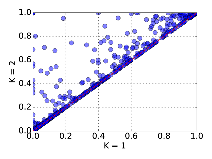
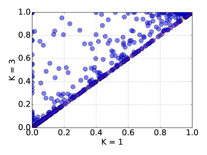
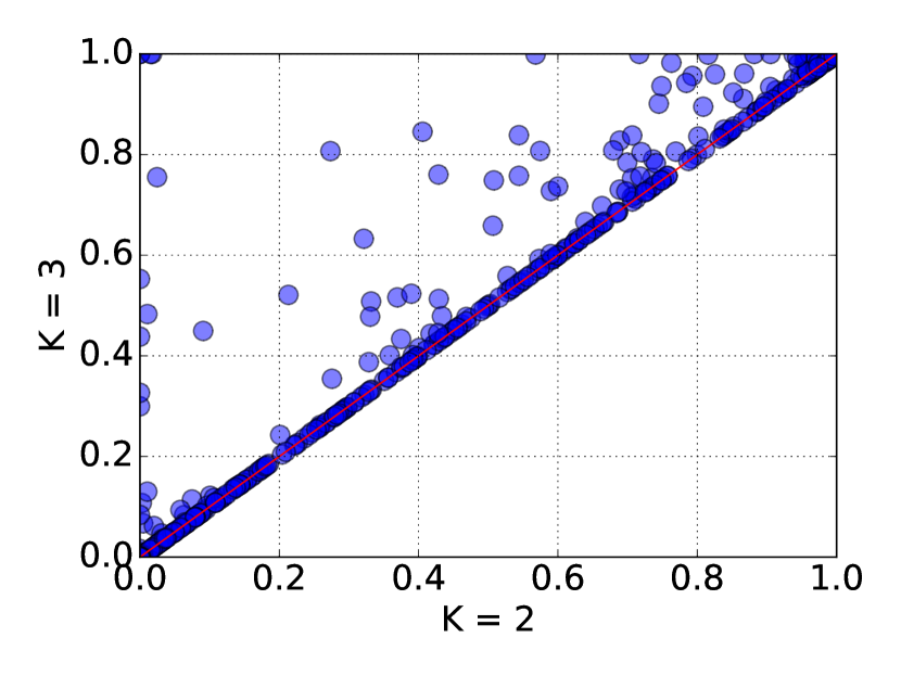
Figure 6: Scatter plot comparing the root gap closed values of the ROOTGAP experiment comparing $(K=1,K=2)$, $(K=1,K=3)$, and $(K=2,K=3)$. For example, each point $(x,y)\in[0,1]^{2}$ in the top left plot corresponds to an instance for which $100x$% of the gap is closed by $K=1$ and $100y$% closed by $K=2$.

group	# instances	$K=1$	$K=2$	$K=3$
ALL	$633$	$18.4$%	$21.4$%	$23.4$%
$m\geq 10$	$528$	$14.6$%	$16.9$%	$18.4$%
$m\geq 20$	$391$	$10.7$%	$12.3$%	$13.5$%
$m\geq 50$	$229$	$7.1$%	$7.9$%	$8.5$%
AFFECTED
ALL	$469$	$35.0$%	$42.2$%	$46.9$%
$m\geq 10$	$370$	$30.1$%	$36.0$%	$40.1$%
$m\geq 20$	$244$	$26.2$%	$31.5$%	$35.4$%
$m\geq 50$	$115$	$23.9$%	$28.0$%	$30.8$%

Table 1: Aggregated results for the ROOTGAP experiment. A row $m\geq x$ considers all instances that have at least $x$ many nonlinear constraints. The second part of the table only considers instances for which at least one setting closes at least $1$% of the root gap.

BENDERS Experiment.

Table 2 reports aggregated results for the BENDERS experiment, which, similar to Figure 6, are visualized in Figure 7. We refer to Table LABEL:table:algo:detailed in the appendix for detailed instance-wise results.

First, we observe that the DEFAULT performs significantly better than PLAIN. Table 2 shows that on $100$ of the $457{}$ affected instances DEFAULT closes at least 1% more gap than PLAIN. Only on $36$ instances PLAIN closes more gap, but over all instances it closes on average ${{}{}{}{}{}{}{}{}{}{}}{{{}{}{}{}{}}}13.1\%$ less gap than DEFAULT. On instances with a larger number of nonlinear constraints, DEFAULT performs even better: on the $107$ instances with at least $50$ nonlinear constraints, DEFAULT computes $35$ times a better and only $1$ time a worse dual bound than PLAIN. For these $107$ instances, PLAIN closes ${{}{}{}{}{}{}{}{}{}{}}{{{}{}{}{}{}}}25.8$% less gap than DEFAULT. Interestingly, Figure 7 shows that there are instances for which PLAIN could not close any gap but DEFAULT could. There is no instance for which the opposite is true.

Next, we analyze which components of the Benders algorithm are responsible for the significantly better performance of DEFAULT compared to PLAIN. Table 2 shows that DEFAULT dominates NOSTAB, NOSUPP, and NOEARLY with respect to the average gap closed and the difference between the number of wins and the number of losses on each subset of the instances. The most important component is the early termination of the master problem. By disabling this feature, the Benders algorithm closes ${{}{}{}{}{}{}{}{}{}{}}{{{}{}{}{}{}}}11.8$% less gap on all instances and even ${{}{}{}{}{}{}{}{}{}{}}{{{}{}{}{}{}}}23.7$% on those which have at least $50$ nonlinear constraints.

Even though Table 2 suggests that the trust-region and support stabilization are not crucial for closing a significant portion of the root gap, both techniques are important to exploit the $\lambda$ space in a more structured way. Once an improving $\lambda$ vector is found, it is likely that there are even better vectors in its neighborhood. The proposed stabilization methods help us to explore this neighborhood and to converge to a local optimum. Overall, this helps us to find better aggregation vectors faster. To visualize this, we use the instance genpooling_lee1 from Example 4. Figure 8 shows the achieved dual bounds and the sparsity pattern of the $\lambda$ vector in each iteration of the Benders algorithm for DEFAULT and NOSTAB. Both settings run with an iteration limit of $600$.

First, we observe that the achieved dual bound of $-4775.26$ with DEFAULT is significantly better than the dual bound of $-5006.95$ when using NOSTAB. The best dual bound is found after $97$ iterations by DEFAULT and after $494$ iterations with NOSTAB. To understand this behavior, we analyze the computed aggregation vectors in each iteration. After DEFAULT finds an aggregation that improves the dual bound, it fixes the support of the aggregation vector and tries to improve the dual bound by finding a better aggregation vector for that fixed support. This happens at the beginning of the solving process and after iteration $62$, which is visible in the bottom left plot of Figure 8. After iteration $112$ the algorithm removed the trust region and support fixation and no further dual bound improvement could be found. Due to the nature of the Benders algorithm, the algorithm frequently oscillates in the $\lambda$ space if no stabilization is used. This is displayed in the “noisy” parts of the $\lambda$ plots of DEFAULT and NOSTAB in Figure 8. In the iterations where no stabilization is used by DEFAULT, we do not observe any pattern indicating which of the two settings finds a better dual bound —the behavior seems rather random. This type of randomness and the large time limit used explain the similar results for the achieved gap closed values for DEFAULT and NOSTAB that are reported in Table 2. The important observation is that using the presented stabilization methods allows us to reach the final dual bound much faster than without using stabilization.

		PLAIN			NOSTAB			NOSUPP			NOEARLY
group	$|P|$	M	L	rgc	M	L	rgc	M	L	rgc	M	L	rgc
ALL	$457$	$100$	$36$	$86.9$	$40$	$31$	$98.3$	$41$	$27$	$98.4$	$94$	$40$	$88.2$
$m\geq 10$	$346$	$90$	$29$	$84.1$	$34$	$27$	$98.7$	$38$	$24$	$98.5$	$85$	$33$	$85.4$
$m\geq 20$	$222$	$72$	$10$	$77.2$	$25$	$17$	$98.5$	$32$	$20$	$98.2$	$65$	$12$	$79.7$
$m\geq 50$	$107$	$35$	$1$	$74.2$	$13$	$7$	$98.9$	$14$	$12$	$98.4$	$32$	$2$	$76.3$

Table 2: Table shows aggregated results for the BENDERS experiment. The column “M”/“L” reports the number of instances for which DEFAULT could close at least 1% more/less root gap than the settings of the corresponding column. Column “rgc” reports the average root gap closed relative to our default settings (in %). Instances for which no setting could close at least 1% of the root gap are filtered out.

(a) PLAIN

(b) NOSTAB

(c) NOSUPP

(d) NOEARLY

Figure 7: Scatter plots comparing the achieved root gap closed values for different settings of the Benders algorithm. The y-axis reports the gap closed values for DEFAULT and the x-axis the gap closed values for the mentioned setting.

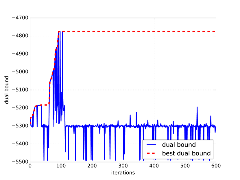
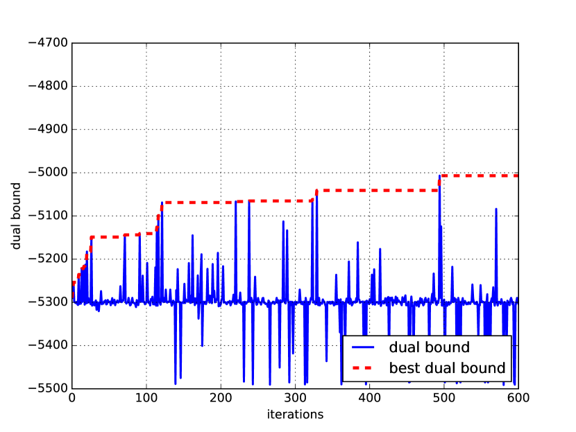
Figure 8: Comparison of the achieved dual bounds and the obtained aggregation vectors during Algorithm 2 for DEFAULT (left) and NOSTAB (right) on genpooling_lee1 using $K=3$. The red dashed curve shows the best found dual bound so far, whereas the blue curve shows the computed dual bound in every iteration. The pictures at the bottom visualize the $\lambda$ vector. White means that an entry $\lambda_{i}$ is zero and blue means that it is one.

DUALBOUND Experiment.

For this experiment, we include all instances which could not be solved by SCIP with default settings within three hours, have a final gap of at least ten percent, terminate without an error, and contain at least four nonlinear constraints. To compute gaps we use the best known primal bounds from the MINLPLib as reference values. This leaves in total $209$ instances for the DUALBOUND experiment. Table LABEL:table:algo:detailed in the appendix reports detailed results on the subset of instances for which the Algorithm 2 was able to improve on the bound obtained by SCIP with default settings, which was the case for $53$ of the $209$ instances. On these instances, the average gap of $284.3$% for SCIP with default settings could be reduced to an average gap of $142.8$%.

Two interesting subsets of instances are the rsyn* and syn* instances. These instances contain a large number of integer variables and linear constraints but all nonlinear constraints are convex. Note that in this case the aggregation constraints remain convex and thus each sub-problem in the Algorithm 2 is a convex optimization problem with integrality constraints. The advantage of using a surrogate relaxation for these problems is that such relaxation is able to capture the important nonlinear structure of the problem using a small convex problem that can be solved substantially faster with branch and bound. This explains the better dual bounds compared to default SCIP after three hours.

Algorithm 2 computes strong dual bounds on difficult nonconvex MINLPs: For example, for all polygon* instances and four facloc* instances, we find better bounds than the reported best known dual bounds from the MINLPLib, as shown in Table 3.

instance	best primal	DB (MINLPLib)	DB (SCIP)	DUALBOUND
polygon25	$-0.78$	$-5.80$	$-4.24$	$-3.94$
polygon50	$-0.78$	$-15.27$	$-10.78$	$-8.72$
polygon75	$-0.78$	$-24.87$	$-16.82$	$-13.55$
polygon100	$-0.78$	$-34.00$	$-24.37$	$-19.03$
facloc1_3_95	$12.30$	$4.46$	$5.50$	$5.70$
facloc1_4_80	$7.88$	$0.16$	$0.09$	$0.41$
facloc1_4_90	$10.46$	$0.48$	$0.49$	$1.18$
facloc1_4_95	$11.18$	$0.79$	$1.40$	$2.40$

Table 3: Comparison between the dual bounds computed by SCIP, Algorithm 2, and the best known dual bounds reported in the MINLPLib for all polygon* and four facloc* instances.

In general, we have observed the following behavior of Algorithm 2. Due to the target dual bound, the first iterations are processed quickly because the master problem (15) is easy to solve and SCIP rapidly finds feasible solutions for the sub-problems, which trigger the early termination criterion. After this first phase, the Benders algorithm finds a promising aggregation vector, i.e., SCIP does not find a feasible solution with an objective value below the target dual bound. Interestingly, we observe that $S^{K}(\lambda)$ cannot be solved to global optimality within the time limit for most of the $209$ instances of the DUALBOUND. However, the dual bound obtained by optimizing $S^{K}(\lambda)$ is often significantly better than the dual bound obtained by optimizing (1) when using the same working limits.

7 Surrogate duality during the tree search

In the previous sections, we focused on developing computational techniques that can improve the performance of a dual bounding procedure based on surrogate duality. While the obtained dual bounds are strong, in general complex instances will still require branching in order to solve them to provable optimality. Additionally, even though the presented computational techniques improve the running time of Algorithm 2, it is still too costly to be used in every node of a branch-and-bound tree.

In this section, we present a technique that incorporates Algorithm 2 into spatial branch and bound. The technique focuses on extracting information of a single execution of Algorithm 2 in the root node, and reuses this information during spatial branch and bound.

Let $\Lambda:=\{\lambda_{1},\ldots,\lambda_{L}\}\subseteq\mathbb{R}^{Km}$ be the set of aggregation vectors that have been computed during Algorithm 2 in the root node of the branch-and-bound tree. We consider only those aggregations that imply a tighter dual bound than the MILP relaxation. Instead of using the generalized Benders algorithm in a local node $v$, we select the most promising aggregation vector $\lambda$ from $\Lambda$ and solve $S^{K}_{v}(\lambda)$, which is equal to $S^{K}(\lambda)$ except that the global linear relaxation is replaced with a linear relaxation that is only locally valid in $v$.

We propose the following procedure. If $S^{K}_{v}(\lambda)$ results in a better dual bound than the local MILP relaxation, i.e., $S^{K}_{v}(0)$, then we skip the remaining aggregation vectors in $\Lambda$ and continue with the tree search. If the dual bound does not improve, then we discard $\lambda$ in the sub-tree with root $v$. The intuition behind discarding aggregations as we search down the tree is twofold. First, since the aggregations are computed in the root node, their ability to provide good dual bounds is expected to deteriorate with the increasing depth of an explored node. Second, we would like to alleviate the computational load of checking for too many aggregations as the branch-and-bound tree-size increases. The idea is stated in Algorithm 3.

0:  node $v$, parent node $p$, parent aggregation candidates $C_{p}\subseteq\Lambda$

0:  $D\in\mathbb{R}$ valid dual bound for $v$, aggregation candidates $C_{v}\subseteq C_{p}$

1:  initialize $D\leftarrow S^{K}_{v}(0)$

2:  initialize $C_{v}\leftarrow C_{p}$

3:  for $\lambda\in C_{v}$ do

4:     if $D<S^{K}_{v}(\lambda)$ then

5:        return  $(S^{K}_{v}(\lambda),C_{v})$

6:     else

7:        $C_{v}\leftarrow C_{v}\,\backslash\,\{\lambda\}$

8:     end if

9:  end for

10:  return  $(D,\emptyset)$

Algorithm 3 Surrogate approximation

Figure 9: A visualization of Algorithm 3 for the instance himmel16 of the MINLPLib. The size of the aggregation pool has been limited to three and we used bread-first-search as the node selection strategy. The colors determine $|C_{v}|$ at each node $v$: green for three, blue for two, orange for one, white for zero aggregations. Red square shaped nodes could be pruned by Algorithm 3, i.e., the proven dual bound exceeds the value of an incumbent solution.

Let $C_{v}\subset\Lambda$ denote the candidate aggregations in node $v$. The algorithm assumes $C_{r}=\Lambda$ for the root node $r$. First, the value of the MILP relaxation of node $p$ is computed in Step 1. Each candidate aggregation $\lambda\in C_{p}$ is used to compute a tighter bound for $v$. If $S^{K}_{v}(\lambda)$ improves upon the MILP relaxation, then the algorithm terminates in Step 5. Otherwise, $\lambda$ is discarded from the set of candidates in $v$ (see Step 7). In case no $\lambda\in C_{p}$ leads to a tighter dual bound, the algorithm returns in Step 10 the value of the MILP relaxation and the empty set as the set of aggregation candidates for $v$.

As illustrated for the instance himmel16 in Figure 9, Algorithm 3 might lead to stronger dual bounds in local nodes of the branch-and-bound tree, which could result in a smaller tree. However, for the challenging instances of the DUALBOUND experiment we observed that solving $S^{K}_{v}(\lambda)$ is too costly and almost always runs into the time limit. In these cases, we cannot improve the dual bound. An exception is instance multiplants_mtg1c. The instance contains $28$ nonlinear constraints, $193$ continuous variables, and $104$ integer variables. SCIP with default settings proves a dual bound of $4096.04$, which is improved by Algorithm 2 to $3161.13$. Algorithm 3 can further improve the dual bound to $2935.58$ in the beginning of the search tree. Overall, there were only seven nodes for which Algorithm 3 could improve a local dual bound. Afterward, all aggregation candidates have been filtered out and SCIP processed $491860$ nodes in total. During the exploration of these nodes, SCIP could not improve the dual bound further.

8 Conclusion

In this article, we studied theoretical and computational aspects of surrogate relaxations for MINLPs. We developed the first algorithm to solve a generalization of the surrogate dual problem that allows multiple aggregations of nonlinear constraints. To this end, we adapted a Benders-type algorithm for solving the classic surrogate dual problem to solve its generalization and proved that the algorithm always converges. Besides computational enhancements for solving the classic and generalized surrogate dual problem, we discussed how to exploit surrogate duality in a spatial branch-and-bound solver to obtain strong dual bounds for difficult nonconvex MINLPs.

Our extensive computational study on the heterogeneous set of publicly available instances of the MINLPLib, which used an implementation in the MINLP solver SCIP, showed that exploiting surrogate duality can lead to significantly better dual bounds than using SCIP with default settings. Concretely, solving the classic surrogate dual problem led to a root gap reduction of $18.4$% on all $633$ instances and $35.0$% on $469$ affected instances. The presented generalization of surrogate duality reduced the root gap further, namely by $23.4$% on all instances and by $46.9$% on the affected instances. Additionally, our experiments showed that the presented computational enhancements are important to obtain good dual bounds for problems with a large number of nonlinear constraints. On the $107$ instances with at least $50$ nonlinear constraints, our implementation of the generalized Benders algorithm closed ${{}{}{}{}{}{}{}{}{}{}}{{{}{}{}{}{}}}25.8$% more root gap when our proposed trust region stabilization, support stabilization, and early termination criterion are used. Finally, our tree experiments showed that using the result of Algorithm 2 during the tree search can lead to significantly better dual bounds than solving MINLPs with standard spatial branch and bound. On very difficult MINLPs, we achieved an average gap reduction from $284.3$% to $142.8$%.

Finally, we want to highlight two out of many open questions that remain related to generalized surrogate duality and its application in branch-and-bound solvers. First, consider the case that each constraint of (1) is quadratic, i.e., $g_{i}(x)=x^{\mathsf{T}}Q_{i}x+q_{i}^{\mathsf{T}}x+b_{i}$ for each $i\in\mathcal{M}$. Note that adding the constraints

$$\sum_{i\in\mathcal{M}}\lambda^{k}_{i}Q_{i}\succeq 0$$

for all $k\in\{1,\ldots,K\}$ to the master problem (15) enforces that each sub-problem is a convex mixed-integer quadratically constrained program. This increases the complexity of the master problem but, at the same time, reduces the complexity of the sub-problems. A computational study of surrogate relaxations using this modification would be interesting on instances for which solving the sub-problems is currently too expensive.

Second, it remains an open question how a pure surrogate-based spatial branch-and-bound approach could perform in practice. All generated points $\mathcal{X}\subseteq X$ of a parent node can be used as an initial set of points in a child node, which could be considered as a warm-start strategy. However, it is not clear how branching decisions would affect the dual bounds obtained by solving a surrogate relaxation. Future work might design a branching rule that tries to improve the dual bounds obtained by solving surrogate relaxations.

Appendix

Table 4: Detailed results for ROOTGAP experiments comparing the achieved root gap closed values for $K\in\{1,2,3\}$ for all instances of the MINLPLib [45]. The generalized Benders algorithm is called after processing the root node of the branch-and-bound tree. The reported gap closed values are relative to the root MILP relaxation value and the value of best known primal solution.

cons — total number of nonlinear constraints
obj — objective sense
best primal — best known primal solution
MILP — MILP relaxation value
S — surrogate relaxation value
iter — total number of surrogate master iterations (“tilim”/“iterlim” for the time/iteration limit
gc — gap closed by S w.r.t. “MILP” and “best primal” column
					K=1			K=2			K=3
instance	cons	obj	best primal	MILP	S	iter	gc	S	iter	gc	S	iter	gc
10bar1A	10	min	1674	1638	1674	72	1.00	1674	60	1.00	1674	57	1.00
10bar1B	10	min	1623.09	1587.09	1622.73	65	0.99	1623.09	66	1.00	1623.09	121	1.00
10bar1C	10	min	1623.09	1485.26	1556.9	38	0.52	1571.31	41	0.62	1571.31	37	0.62
10bar1D	10	min	1623.09	1485.26	1536.18	269	0.37	1536.18	26	0.37	1556.4	32	0.52
10bar2	20	min	1954.23	1816.92	1817.28	12	0.00	1817.28	5	0.00	1831.68	21	0.11
4stufen	33	min	116330	100935	101307	128	0.02	101307	2532	0.02	101307	948	0.02
72bar	144	min	75.9049	71.5849	71.5849	249	0.00	71.5849	255	0.00	71.5849	249	0.00
90bar	180	min	97.5374	91.5374	91.5374	190	0.00	91.5374	192	0.00	91.5374	178	0.00
alkyl	7	min	-1.765	-1.99912	-1.77216	18	0.97	-1.77216	5	0.97	-1.77085	7	0.97
alkylation	7	max	1768.81	2446.83	1994.76	10	0.67	1994.76	1	0.67	1994.76	1	0.67
arki0003	1068	min	3795.21	3795.21	3795.21	1019	0.00	3795.21	1338	0.00	3795.21	1147	0.00
arki0010	96	min	-187909	-291475	-290228	10	0.01	-290228	5	0.01	-290228	5	0.01
arki0015	698	min	-272.3	-287.003	-287.003	650	0.00	-287.003	889	0.00	-287.003	844	0.00
arki0016	1983	min	867.973	-1364.98	-1172.52	2	0.09	-1172.52	1	0.09	-1172.52	1	0.09
arki0017	1828	min	-121.833	-1338.23	-1195.86	2	0.12	-1195.86	1	0.12	-1195.86	1	0.12
arki0024	1091	min	-7431.03	1e+20	1e+20	1	0.00	1e+20	1	0.00	1e+20	1	0.00
bayes2_50	55	min	0.520208	1.0781e-13	-1.63425e-13	1704	0.00	-1.63425e-13	2339	0.00	-1.63425e-13	2103	0.00
bchoco05	22	max	0.951903	0.999964	0.966299	16928	0.69	0.966299	3312	0.69	0.966299	1769	0.69
bchoco06	29	max	0.962776	0.999984	0.977224	18723	0.60	0.977224	3888	0.60	0.977224	1813	0.60
blend029	12	max	13.3594	15.1395	14.0064	64	0.64	13.9694	989	0.66	13.9694	736	0.66
blend146	24	max	45.2966	47.5904	47.1457	185	0.19	46.9195	474	0.29	46.9195	429	0.29
blend480	32	max	9.2266	10.0559	9.7054	223	0.42	9.7054	346	0.42	9.7054	336	0.42
blend531	30	max	20.039	20.9269	20.6962	528	0.26	20.6962	1047	0.26	20.6962	604	0.26
blend718	24	max	7.3936	20.3614	19.7031	208	0.05	19.625	581	0.06	19.625	354	0.06
blend721	24	max	13.5268	14.34	14.0342	307	0.38	14.0342	596	0.38	14.0342	393	0.38
blend852	32	max	53.9627	54.4795	54.2402	297	0.46	54.2402	522	0.46	54.2402	381	0.46
btest14	86	min	-59.8174	-185883	-115.308	304	1.00	-115.308	713	1.00	-92.0466	674	1.00
camshape100	100	min	-4.28415	-5.0295	-4.92812	26	0.14	-4.90792	4441	0.16	-4.90792	6625	0.16
camshape200	200	min	-4.2785	-5.15377	-5.1347	9	0.02	-5.09494	421	0.07	-5.09494	400	0.07
camshape400	400	min	-4.2757	-5.24589	-5.24589	1	0.00	-5.24589	2	0.00	-5.23617	4	0.01
camshape800	800	min	-4.27431	-5.31228	-5.31228	0	0.00	-5.31228	0	0.00	-5.31228	0	0.00
carton7	21	min	191.73	134.449	152.117	109	0.31	152.117	388	0.31	152.117	204	0.31
carton9	16	min	205.137	167.885	177.885	93	0.27	177.885	1	0.27	177.885	1	0.27
casctanks	211	min	9.16348	7.30572	1e+20	2	1.00	1e+20	1	1.00	1e+20	1	1.00
cesam2log	42	min	0.50796	-436.696	-394.889	2	0.10	-395.003	1	0.10	-394.964	1	0.10
chenery	23	min	-1058.92	-1177.81	-1074.99	119	0.86	-1062.6	2487	0.97	-1060.43	1283	0.99
chp_partload	481	min	23.2981	20.209	20.209	137	0.00	20.209	122	0.00	20.2134	93	0.00
chp_shorttermplan1a	384	min	214.842	214.296	214.705	249	0.75	214.708	513	0.75	214.708	483	0.75
chp_shorttermplan1b	768	min	254.317	242.356	242.755	11	0.03	242.783	10	0.04	242.791	7	0.04
chp_shorttermplan2a	768	min	245800	240127	244292	727	0.73	244292	1935	0.73	244292	1398	0.73
chp_shorttermplan2d	1344	min	489382	468259	468259	2	0.00	468259	2	0.00	468259	2	0.00
clay0203h	24	min	41573.3	3560	3560	9	0.00	4219.46	1000	0.02	1e+20	93	1.00
clay0203m	24	min	41573.3	3560	3560	2	0.00	3560	8	0.00	24570.6	1398	0.55
clay0205m	40	min	8092.5	8085	8085	6	0.00	8085	24	0.00	8085	36	0.00
clay0303h	36	min	26669.1	3560	3560	14	0.00	4127.95	616	0.02	21008.7	584	0.76
clay0303m	36	min	26669.1	3560	3560	2	0.00	3560	20	0.00	3930	340	0.02
clay0304h	48	min	40262.4	6540	6545	28	0.00	6900	155	0.01	22828.8	243	0.48
clay0304m	48	min	40262.4	6545	6545	3	0.00	6900	142	0.01	10933.1	93	0.13
clay0305h	60	min	8092.5	8085	8085	18	0.00	8085	42	0.00	8092.5	39	1.00
clay0305m	58	min	8092.5	8085	8085	3	0.00	8085	23	0.00	8085	16	0.00
crudeoil_lee1_07	36	max	79.75	80	79.75	0	1.00	79.75	0	1.00	79.75	0	1.00
crudeoil_lee1_08	42	max	79.75	79.7619	79.75	3	0.92	79.75	1	0.92	79.75	2	0.92
crudeoil_lee1_09	48	max	79.75	80	79.75	0	1.00	79.75	0	1.00	79.75	0	1.00
crudeoil_lee1_10	54	max	79.75	80	79.75	0	1.00	79.75	0	1.00	79.75	0	1.00
crudeoil_lee2_09	109	max	101.175	103	101.175	0	1.00	101.175	0	1.00	101.175	0	1.00
crudeoil_lee3_05	106	max	85.4489	87.4	85.5057	147	0.97	85.5057	173	0.97	85.5057	165	0.97
crudeoil_lee3_06	141	max	85.4489	87.4	85.5307	76	0.96	85.5307	101	0.96	85.5307	90	0.96
crudeoil_lee3_07	176	max	85.4489	87.4093	85.5234	98	0.96	85.5234	58	0.96	85.5234	71	0.96
crudeoil_lee3_08	211	max	85.4489	87.4	85.532	60	0.96	85.532	50	0.96	85.532	46	0.96
crudeoil_lee3_09	246	max	85.4489	87.4	85.5232	46	0.96	85.5232	34	0.96	85.5232	37	0.96
crudeoil_lee3_10	281	max	85.4489	87.4	85.5273	33	0.96	85.5273	26	0.96	85.5273	22	0.96
crudeoil_lee4_07	111	max	132.548	132.585	132.548	0	0.96	132.548	0	0.96	132.548	0	0.96
crudeoil_lee4_08	130	max	132.548	132.585	132.551	0	0.89	132.551	0	0.89	132.551	0	0.89
crudeoil_lee4_09	149	max	132.548	132.585	132.585	0	0.00	132.585	0	0.00	132.585	0	0.00
crudeoil_lee4_10	168	max	132.548	132.585	132.548	0	0.96	132.548	0	0.96	132.548	0	0.96
crudeoil_li02	15	max	1.01567e+08	1.02699e+08	1.02694e+08	13	0.00	1.02685e+08	1	0.01	1.02685e+08	1	0.01
crudeoil_li03	192	max	3483.65	3541.05	3532.41	2	0.15	3531.85	1	0.16	3531.89	1	0.16
crudeoil_li05	192	max	3129.84	3390.47	3389.97	56	0.00	3389.28	48	0.00	3372.97	41	0.07
crudeoil_li11	192	max	4686.79	4720.79	4720.79	5	0.00	4720.79	5	0.00	4720.79	4	0.00
crudeoil_li21	192	max	4799.58	4869.83	4869.83	2	0.00	4869.83	2	0.00	4869.83	2	0.00
crudeoil_pooling_ct1	37	min	210538	132173	160092	2	0.36	160093	1	0.36	160121	1	0.36
crudeoil_pooling_ct2	70	max	10246.2	10616	10557.8	68	0.16	10528.8	40	0.24	10528.8	35	0.24
crudeoil_pooling_ct3	182	min	287000	180144	228317	2	0.45	228327	1	0.45	228368	1	0.45
crudeoil_pooling_ct4	95	max	13258.2	14123.1	14036.7	53	0.10	14036	46	0.10	14017.7	37	0.12
crudeoil_pooling_dt1	570	min	209585	209585	209585	18	0.00	209585	19	0.00	209585	16	0.00
crudeoil_pooling_dt2	1106	max	10239.9	11598.1	11598.1	1	0.00	11600.8	1	0.00	11611	1	0.00
crudeoil_pooling_dt3	2707	min	284781	284781	284781	4	0.00	284781	4	0.00	284781	4	0.00
crudeoil_pooling_dt4	1121	max	13257.6	14332.4	14332.4	1	0.00	14332.4	1	0.00	14332.4	1	0.00
cvxnonsep_nsig30r	30	min	156.427	156.402	156.411	0	0.35	156.411	0	0.35	156.411	0	0.35
cvxnonsep_psig20r	21	min	95.8974	95.8862	95.8873	0	0.09	95.8873	0	0.09	95.8873	0	0.09
cvxnonsep_psig30r	31	min	78.9989	30	54.6322	64108	0.50	54.6322	13309	0.50	54.6322	12019	0.50
cvxnonsep_psig40r	41	min	86.5451	67.5396	67.5663	17568	0.00	67.5663	18569	0.00	67.5752	16	0.00
deb10	64	min	209.428	0	0	7706	0.00	0	2805	0.00	0	1801	0.00
deb6	246	min	201.739	0	0	1825	0.00	0	2121	0.00	0	1978	0.00
deb7	420	min	116.585	0	0	1387	0.00	0	1756	0.00	0	1194	0.00
deb8	420	min	116.585	0	0	1467	0.00	0	2128	0.00	0	1094	0.00
deb9	420	min	116.585	0	0	1468	0.00	0	2037	0.00	1e+20	832	1.00
elec100	101	min	4448.35	1750.09	1750.09	2	0.00	1750.09	2	0.00	1750.09	2	0.00
elec25	26	min	243.813	106.066	106.066	2	0.00	106.066	2	0.00	106.066	2	0.00
elec50	51	min	1055.18	433.103	433.103	2	0.00	433.103	2	0.00	433.103	2	0.00
elf	27	min	0.191667	0	0	10	0.00	0	2549	0.00	0	536	0.00
eq6_1	29	min	670.694	-5.78483e-07	21.8033	3	0.03	21.7877	1	0.03	21.7	1	0.03
estein1_t4Nr22	9	min	0.503284	0.0327137	0.111554	23	0.17	0.235008	80	0.43	0.27469	75	0.51
estein1_t5Nr1	18	min	1.6644	0	0	33	0.00	0	77	0.00	0	178	0.00
estein1_t5Nr21	18	min	1.81818	0	0.0198308	46	0.01	0.115163	308	0.06	0.151745	501	0.08
estein4_data1	9	min	0.801363	0.0127965	0.0807117	37	0.09	0.215665	26	0.26	0.215665	85	0.26
estein4_data2	9	min	1.18808	0.0359439	0.201269	31	0.14	0.468235	129	0.37	0.535823	329	0.43
estein4_data3	9	min	1.07269	0.103197	0.173716	22	0.07	0.391958	45	0.30	0.391958	2	0.30
estein5_data1	18	min	1.04537	0	0	21	0.00	0	127	0.00	0	196	0.00
estein5_data2	18	min	1.19316	0	0	18	0.00	0.0239539	280	0.02	0.0737598	686	0.06
estein5_data3	18	min	1.49908	0	0	23	0.00	0.112064	194	0.07	0.171853	286	0.11
etamac	10	min	-15.2947	-16.9614	-16.0355	12	0.56	-16.0056	12	0.57	-15.9735	1	0.59
ex1263a	4	min	19.6	19.1	19.3	8	0.40	19.6	125	1.00	19.6	13	1.00
ex1264a	4	min	8.6	8.3	8.3	8	0.00	8.6	57	1.00	8.6	19	1.00
ex3_1_1	3	min	7049.25	2835.87	5927.41	58	0.73	6789.38	116	0.94	7043.1	5	1.00
ex3_1_2	3	min	-30665.5	-30665.5	-30665.5	0	0.00	-30665.5	0	0.00	-30665.5	0	0.00
ex3_1_3	3	min	-310	-310.542	-310	1	1.00	-310	0	1.00	-310	0	1.00
ex3pb	5	min	68.0097	67.6674	67.9862	0	0.93	67.9862	0	0.93	67.9862	0	0.93
ex4_1_9	2	min	-5.50801	-6.98879	-5.76657	40	0.82	-5.51045	5	1.00	-5.51045	0	1.00
ex5_2_2_case1	3	min	-400	-2075.65	-565.614	63	0.90	-565.614	497	0.90	-565.603	606	0.90
ex5_2_2_case2	3	min	-600	-2699.71	-1199.47	853	0.71	-1194.87	2506	0.72	-600	62	1.00
ex5_2_2_case3	3	min	-750	-2018.9	-817.661	35	0.95	-801.899	73	0.96	-750.662	2	1.00
ex5_2_4	4	min	-450	-550	-450.154	34	1.00	-450.154	13	1.00	-450.154	8	1.00
ex5_3_2	9	min	1.86416	0.9979	1.51809	123	0.60	1.85845	3733	0.99	1.85845	1099	0.99
ex5_3_3	35	min	3.23402	1.77589	1.97431	40	0.14	2.03472	54	0.18	2.03563	1	0.18
ex5_4_2	3	min	7512.23	3100.82	6622.19	76	0.80	6698.07	18471	0.82	7505.67	5	1.00
ex5_4_3	5	min	4845.46	4218.8	4845.46	13	1.00	4845.46	0	1.00	4845.46	0	1.00
ex5_4_4	7	min	10077.8	4294.25	8884.32	104	0.79	9817.59	295	0.96	9971.9	178	0.98
ex6_1_1	5	min	-0.0201983	-4.91971	-0.669569	5670	0.87	-0.669569	4665	0.87	-0.210453	2852	0.96
ex6_1_2	3	min	-0.0324638	-3.7935	-0.411122	299	0.90	-0.0813333	1031	0.99	-0.032465	31	1.00
ex6_1_3	7	min	-0.352498	-5.16504	-2.60598	2	0.53	-2.60597	1	0.53	-2.60602	1	0.53
ex7_2_1	11	min	1227.23	1088.82	1215.24	16	0.91	1215.24	13	0.91	1217.18	13	0.93
ex7_2_2	5	min	-0.388811	-0.503991	-0.423536	52	0.69	-0.394663	178	0.94	-0.394663	210	0.94
ex7_2_3	3	min	7049.25	2100	4186.98	7	0.42	4186.98	1	0.42	4186.98	1	0.42
ex7_2_4	5	min	3.91801	1.20593	3.25283	42	0.75	3.71573	90	0.93	3.71573	120	0.93
ex7_3_3	2	min	0.817529	0	0.52484	17	0.64	1e+20	5	1.00	1e+20	1	1.00
ex7_3_4	7	min	6.27463	0	0	43	0.00	3.43474	1806	0.55	3.43474	562	0.55
ex7_3_5	11	min	1.20687	0	-1.11022e-16	26	0.00	-1.11022e-16	87	0.00	-1.11022e-16	129	0.00
ex8_1_7	4	min	0.0293108	-114.652	-0.164832	101	1.00	-0.078817	157	1.00	-0.078817	261	1.00
ex8_2_1b	28	min	-979.178	-980.168	1e+20	178	1.00	1e+20	1	1.00	1e+20	1	1.00
ex8_2_2b	1552	min	-552.666	-582.755	-581.99	443	0.03	-581.99	507	0.03	-581.99	472	0.03
ex8_2_3b	1819	min	-3731.08	-3731.6	-3731.6	962	0.00	-3731.6	1342	0.00	-3731.6	1280	0.00
ex8_2_4b	60	min	-1197.13	-1197.5	-1197.5	202	0.00	-1197.5	2413	0.00	-1197.5	2319	0.00
ex8_2_5b	3103	min	-830.338	-850.786	-848.573	442	0.11	-848.573	474	0.11	-848.573	447	0.11
ex8_3_1	59	min	-0.81959	-1	1e+20	165	1.00	1e+20	1	1.00	1e+20	1	1.00
ex8_3_11	59	min	-0.799572	-1	-1	10344	0.00	1e+20	103	1.00	1e+20	1	1.00
ex8_3_13	54	min	-43.0895	-49.8432	-49.8432	4605	0.00	-49.8432	1643	0.00	-49.8432	664	0.00
ex8_3_2	49	min	-0.41233	-0.58	-0.58	11428	0.00	-0.58	5259	0.00	-0.58	3498	0.00
ex8_3_3	49	min	-0.416603	-0.58	-0.58	7903	0.00	-0.58	3957	0.00	-0.58	3427	0.00
ex8_3_4	49	min	-3.57998	-5.8	-5.8	5051	0.00	-5.8	3343	0.00	-5.8	2384	0.00
ex8_3_5	49	min	-0.0691197	-1	-1	11901	0.00	-1	3713	0.00	-1	3069	0.00
ex8_3_8	65	min	-3.25612	-5.7	-5.7	3026	0.00	-5.7	2418	0.00	-5.7	2228	0.00
ex8_3_9	27	min	-0.763002	-1	-1	1062	0.00	-1	2721	0.00	-1	1622	0.00
ex8_4_1	11	min	0.618573	0.424552	0.424552	181	0.00	0.424552	2987	0.00	0.424552	2879	0.00
ex8_4_2	11	min	0.485152	-5.20839e-07	-5.20839e-07	151	0.00	-5.20839e-07	2921	0.00	-5.20839e-07	1169	0.00
ex8_4_3	26	min	0.00464972	-5.20436e-07	-5.20436e-07	357	0.00	-5.20436e-07	2942	0.00	-5.20436e-07	1990	0.00
ex8_4_4	13	min	0.21246	0.055808	0.146442	284	0.57	0.151382	1657	0.61	0.151382	930	0.61
ex8_4_7	41	min	29.0473	23.6129	23.6129	89	0.00	23.6129	1800	0.00	23.6129	689	0.00
ex8_5_1	3	min	-4.072e-07	-8.49028	-0.279007	34	0.97	-0.00121038	70	1.00	-1.13414e-06	21	1.00
ex9_2_3	6	min	-0	-30	0	11	1.00	0	4	1.00	0	4	1.00
ex9_2_5	4	min	5	-3.43839e-07	5	6	1.00	5	5	1.00	5	4	1.00
filter	2	min	8685.28	8685.26	8685.26	2	0.00	8685.26	2	0.00	8685.26	2	0.00
flay02h	2	min	37.9473	32.9167	37.9061	12	0.99	37.9473	3	1.00	37.9473	0	1.00
flay02m	2	min	37.9473	34.1794	37.9298	14	1.00	37.9421	2	1.00	37.9421	0	1.00
flay03h	3	min	48.9898	38.8308	47.1516	25	0.82	47.7877	1950	0.88	48.9898	8	1.00
flay03m	3	min	48.9898	39.4574	47.2876	30	0.82	48.0865	2962	0.91	48.9898	2	1.00
flay04h	4	min	54.4059	48.4665	52.7386	36	0.72	53.6106	743	0.87	53.8758	476	0.91
flay04m	4	min	54.4059	47.779	53.1398	29	0.81	53.4234	1754	0.85	53.8972	594	0.92
flay05h	5	min	64.4981	49.9829	60.09	40	0.70	60.6767	66	0.74	61.4541	64	0.79
flay05m	5	min	64.4981	46.9222	59.8493	70	0.74	60.4413	460	0.77	61.0858	324	0.81
flay06h	6	min	66.9328	47.9208	58.7592	15	0.57	59.8598	14	0.63	59.9685	6	0.63
flay06m	6	min	66.9328	47.8418	60.8425	34	0.68	61.8808	17	0.74	62.2253	31	0.75
fo7	14	min	20.7298	16.7051	20.7121	250	1.00	20.718	283	1.00	20.7244	306	1.00
fo7_2	14	min	17.7493	15.2564	17.7486	176	1.00	17.7493	293	1.00	17.7493	81	1.00
fo7_ar25_1	14	min	23.0936	21.2923	23.0867	176	1.00	23.0897	193	1.00	23.0913	261	1.00
fo7_ar2_1	14	min	24.8398	22.9076	24.82	57	0.99	24.8355	302	1.00	24.8395	42	1.00
fo7_ar3_1	14	min	22.5175	19.6488	22.3846	57	0.95	22.4847	79	0.99	22.4847	121	0.99
fo7_ar4_1	14	min	20.7298	18.0191	20.7118	129	0.99	20.7247	233	1.00	20.7247	230	1.00
fo7_ar5_1	14	min	17.7493	15.2564	17.7482	129	1.00	17.7482	361	1.00	17.7492	334	1.00
fo8	16	min	22.3819	22.2518	22.3262	19	0.57	22.3435	19	0.70	22.3546	24	0.78
fo8_ar25_1	16	min	28.0452	22.9102	27.27	32	0.85	27.912	20	0.97	28.0023	98	0.99
fo8_ar2_1	16	min	30.3406	27.2512	30.0864	24	0.92	30.2062	31	0.96	30.2941	53	0.98
fo8_ar3_1	16	min	23.9101	23.1017	23.8396	94	0.91	23.8606	72	0.94	23.8707	75	0.95
fo8_ar4_1	16	min	22.3819	20.25	22.2978	123	0.96	22.355	112	0.99	22.355	111	0.99
fo8_ar5_1	16	min	22.3819	19.8671	22.021	61	0.86	22.316	64	0.97	22.316	68	0.97
fo9	18	min	23.4643	23.1845	23.2869	7	0.36	23.3501	9	0.59	23.3888	10	0.73
fo9_ar25_1	18	min	32.1864	23.8753	29.7925	12	0.71	29.7925	12	0.71	29.7925	10	0.71
fo9_ar2_1	18	min	32.625	30.7921	31.5205	6	0.40	31.5205	3	0.40	31.5205	3	0.40
fo9_ar3_1	18	min	24.8155	23.0745	24.8126	5	1.00	24.8126	48	1.00	24.8126	40	1.00
fo9_ar4_1	18	min	23.4643	21.7767	23.3213	29	0.91	23.3213	42	0.91	23.3213	32	0.91
fo9_ar5_1	18	min	23.4643	21.703	23.1005	13	0.79	23.1005	12	0.79	23.3884	17	0.96
gabriel01	48	max	45.2444	47.3515	46.65	212	0.33	46.65	428	0.33	46.65	328	0.33
gabriel02	96	max	39.6097	46.8201	45.7175	120	0.15	45.7175	203	0.15	45.7175	195	0.15
gabriel09	288	max	112.42	134.475	134.4	29	0.00	134.4	25	0.00	134.4	20	0.00
gams01	111	min	21380.2	474.611	474.611	1	0.00	474.581	1	0.00	474.511	1	0.00
gams02	193	min	8.94669e+07	2.03571e+06	5.16771e+06	10	0.04	7.11317e+06	6	0.06	1.02315e+07	5	0.09
gasnet_al2	191	min	7114.13	6150.81	6321.3	24	0.18	6321.5	1	0.18	6321.57	1	0.18
gasnet_al3	191	min	7363.32	6282.7	6680.1	9	0.37	6680.1	1	0.37	6680.1	1	0.37
genpool04	15	min	1.28564e+06	706715	854295	94	0.25	866245	141	0.28	911908	81	0.35
genpool10	33	min	2.0748e+06	707408	819149	22	0.08	821563	15	0.08	821563	29	0.08
genpool10i	300	min	1.19809e+06	707063	830210	20	0.25	834009	28	0.26	835898	14	0.26
genpool10paper	33	min	1.16851e+06	707408	843449	12	0.30	843449	33	0.30	843449	35	0.30
genpool15	48	min	991560	587181	732152	78	0.36	732152	109	0.36	749303	68	0.40
genpool15i	675	min	992088	698353	751814	59	0.18	779835	45	0.28	779835	54	0.28
genpool15paper	48	min	3.03513e+06	586695	735273	79	0.06	744062	89	0.06	744062	80	0.06
genpool20	66	min	1.34268e+06	702568	845308	41	0.22	889770	73	0.29	889770	77	0.29
genpool20i	1260	min	1.48782e+06	954287	990234	36	0.07	995844	30	0.08	995844	31	0.08
genpooling_lee1	20	min	-4640.08	-5289.7	-5198	106	0.14	-4936.34	707	0.54	-4744.96	453	0.84
genpooling_meyer15	48	min	943734	678910	700248	9	0.08	700248	1	0.08	700248	1	0.08
haverly	3	min	-400	-2081.45	-573.213	79	0.90	-400	182	1.00	-400	0	1.00
himmel11	4	min	-30665.5	-30665.5	-30665.5	0	0.00	-30665.5	0	0.00	-30665.5	0	0.00
himmel16	19	min	-0.866025	-3.5	-1.99694	13	0.57	-1.63011	52	0.71	-1.60499	1	0.72
house	3	min	-4500	-4671.88	-4504.13	49	0.98	-4504.13	16	0.98	-4503.45	16	0.98
hs62	2	min	-26272.5	-87205.5	-26297.7	1	1.00	-26297.7	0	1.00	-26297.7	0	1.00
hvb11	17	min	46962	38668.9	46957.5	65	1.00	46957.5	2416	1.00	46957.5	732	1.00
hybriddynamic_var	3	min	1.53642	1.4743	1.53489	1	0.96	1.53489	0	0.96	1.53489	0	0.96
hybriddynamic_varcc	21	min	1.53642	1.11087	1.53489	1	0.99	1.53489	0	0.99	1.53489	0	0.99
hydroenergy1	46	max	209721	213710	210918	80	0.70	210756	52	0.74	210587	63	0.78
hydroenergy2	92	max	371812	379535	377716	15	0.24	377630	18	0.25	377618	26	0.25
hydroenergy3	161	max	744964	763977	761859	17	0.11	761847	1	0.11	761847	1	0.11
ibs2	10	min	4.45285	4.38555	4.39031	8	0.07	4.43377	8	0.71	4.43441	1	0.72
johnall	191	min	-224.73	-227.025	-224.76	2612	0.99	-224.76	5	0.99	-224.76	5	0.99
kall_circles_c6a	22	min	2.11172	0	0	95	0.00	0	339	0.00	0	272	0.00
kall_circles_c6b	22	min	1.9736	0	0	70	0.00	0	453	0.00	0	305	0.00
kall_circles_c6c	29	min	2.7977	0	0	26	0.00	0	356	0.00	0	302	0.00
kall_circles_c7a	29	min	2.66281	0	0	45	0.00	0	591	0.00	0	332	0.00
kall_circles_c8a	37	min	2.54092	0	0	31	0.00	0	420	0.00	0	290	0.00
kall_circlespolygons_c1p12	21	min	0.339602	0	0	318	0.00	0	1493	0.00	0	683	0.00
kall_circlespolygons_c1p13	21	min	0.339602	0	0	308	0.00	0	1296	0.00	0	911	0.00
kall_circlespolygons_c1p5a	106	min	2.84872	0	0	3975	0.00	0	4457	0.00	0	1489	0.00
kall_circlespolygons_c1p5b	631	min	3.87051	0	0	1207	0.00	0	3704	0.00	0	2497	0.00
kall_circlespolygons_c1p6a	904	min	3.84872	0	0	1061	0.00	0	3564	0.00	0	2108	0.00
kall_circlesrectangles_c1r12	23	min	0.339602	0	0	389	0.00	0	1141	0.00	0	1164	0.00
kall_circlesrectangles_c1r13	23	min	0.214602	0	0	359	0.00	0	1144	0.00	0	873	0.00
kall_circlesrectangles_c6r1	133	min	7.1645	0	0	3387	0.00	0	4357	0.00	0	1521	0.00
kall_circlesrectangles_c6r29	283	min	6.29517	0	0	1983	0.00	0	4736	0.00	0	1968	0.00
kall_circlesrectangles_c6r39	466	min	6.63339	0	0	1418	0.00	0	5265	0.00	0	1619	0.00
kall_congruentcircles_c31	4	min	0.643806	0	0	20	0.00	0.00981198	7820	0.02	1e+20	78	1.00
kall_congruentcircles_c32	4	min	1.37586	0	0.596951	50	0.43	1.05032	5586	0.76	1.35274	1197	0.98
kall_congruentcircles_c41	6	min	0.858407	0	0	14	0.00	0.488053	7664	0.57	0.858348	8	1.00
kall_congruentcircles_c42	7	min	0.858407	0	0	30	0.00	0.276102	3154	0.32	0.543757	648	0.63
kall_congruentcircles_c51	11	min	1.07301	0	0	30	0.00	0	651	0.00	0	268	0.00
kall_congruentcircles_c52	11	min	1.53711	0	0	68	0.00	0	1262	0.00	0.460982	471	0.30
kall_congruentcircles_c61	16	min	1.28761	0	0	13	0.00	0	491	0.00	0	315	0.00
kall_congruentcircles_c62	16	min	1.28761	0	0	56	0.00	0	957	0.00	0.420744	519	0.33
kall_congruentcircles_c63	16	min	1.28761	0	0	32	0.00	0	964	0.00	0.108015	600	0.08
kall_congruentcircles_c71	22	min	1.50221	0	0	7	0.00	0	501	0.00	0	236	0.00
kall_congruentcircles_c72	22	min	1.96631	0	0	33	0.00	0	1004	0.00	0	440	0.00
kall_diffcircles_10	45	min	11.9355	-1e-09	-1e-09	19	0.00	-1e-09	56	0.00	-1e-09	114	0.00
kall_diffcircles_5a	11	min	5.11618	1.88496	2.04174	33	0.05	3.52664	2145	0.51	4.30481	230	0.75
kall_diffcircles_5b	11	min	5.11618	0	2.04226	73	0.40	2.93947	2383	0.57	4.13018	368	0.81
kall_diffcircles_6	16	min	7.78789	0	0	54	0.00	5.36454	2401	0.69	6.44673	294	0.83
kall_diffcircles_7	22	min	7.15313	0	0	152	0.00	3.06524	514	0.43	5.43874	247	0.76
kall_diffcircles_8	28	min	14.4813	-1e-09	-1e-09	15	0.00	-1e-09	66	0.00	-1e-09	122	0.00
kall_diffcircles_9	36	min	13.3503	-1e-09	-1e-09	49	0.00	-1e-09	144	0.00	-1e-09	170	0.00
kall_ellipsoids_tc02b	48	min	32.4	22.5	22.5	684	0.00	22.5	1608	0.00	22.5	907	0.00
kall_ellipsoids_tc03c	74	min	36.4536	18.9752	18.9752	845	0.00	18.9752	883	0.00	18.9752	528	0.00
kall_ellipsoids_tc05a	321	min	39.3979	20.9921	20.9921	1688	0.00	20.9921	1280	0.00	20.9921	646	0.00
knp3-12	78	max	1.10557	8	4.93324	12	0.44	4.93324	6	0.44	4.93324	6	0.44
knp4-24	300	max	1	10	10	14	0.00	8.76316	4	0.14	8.75145	1	0.14
knp5-40	820	max	0.984855	12	12	22	0.00	12	21	0.00	12	18	0.00
knp5-41	861	max	0.968886	12	12	23	0.00	12	19	0.00	12	16	0.00
knp5-42	903	max	0.960072	12	12	24	0.00	12	23	0.00	12	20	0.00
knp5-43	946	max	0.947522	12	12	24	0.00	12	21	0.00	12	13	0.00
knp5-44	990	max	0.944767	12	12	24	0.00	12	23	0.00	12	21	0.00
kport20	20	min	31.8093	28.4678	29.5943	49	0.34	29.9199	52	0.43	29.9199	67	0.43
kport40	38	min	37.1758	31.7627	32.1351	38	0.07	32.2835	22	0.10	32.3156	1	0.10
launch	13	min	2257.8	1767.15	2257.78	28590	1.00	2257.78	5979	1.00	2257.79	3790	1.00
lnts100	400	min	0.554595	0.504006	0.507421	66	0.07	0.507421	69	0.07	0.507421	41	0.07
lnts200	800	min	0.554577	0.503132	0.504579	134	0.03	0.504579	64	0.03	0.504579	41	0.03
lnts50	200	min	0.554669	0.5039	0.511237	83	0.14	0.511237	28	0.14	0.511237	21	0.14
lop97ic	40	min	4041.83	3921.07	3923.69	31	0.02	3923.69	25	0.02	3923.69	20	0.02
lop97icx	40	min	4099.06	4053.82	4067.3	192	0.30	4067.3	169	0.30	4067.3	152	0.30
m3	6	min	37.8	11.5096	37.8	0	1.00	37.8	0	1.00	37.8	0	1.00
m6	12	min	82.2569	81.7964	82.2569	15	1.00	82.2569	6	1.00	82.2569	6	1.00
m7	14	min	106.757	102.703	106.757	53	1.00	106.757	7	1.00	106.757	7	1.00
m7_ar25_1	14	min	143.585	139.928	143.585	84	1.00	143.585	2	1.00	143.585	0	1.00
m7_ar2_1	14	min	190.235	170.157	190.224	60	1.00	190.235	740	1.00	190.235	133	1.00
m7_ar3_1	14	min	143.585	127.379	143.583	49	1.00	143.585	55	1.00	143.585	0	1.00
m7_ar4_1	14	min	106.757	56.463	106.757	0	1.00	106.757	0	1.00	106.757	0	1.00
m7_ar5_1	14	min	106.46	98.8972	106.46	2	1.00	106.46	0	1.00	106.46	0	1.00
mathopt1	2	min	0	-693.773	-1.79768e-07	2	1.00	-1.7959e-07	1	1.00	-1.79682e-07	1	1.00
mathopt4	2	min	0	-391.807	-2.19008e-07	2	1.00	-2.1863e-07	1	1.00	-2.18459e-07	1	1.00
maxmin	78	min	-0.366096	-1.1547	-0.947326	60	0.26	-0.934078	46	0.28	-0.934078	45	0.28
mbtd	20	min	4.66666	2.5	2.61274	6	0.05	2.61274	4	0.05	2.61274	4	0.05
meanvar-orl400_05_e_7	401	min	99.4826	6.13347	19.9457	9	0.15	19.9457	1	0.15	19.9457	1	0.15
mpss-basic-ob25-125-125	24	max	0	102.818	102.396	4	0.00	102.337	3	0.00	102.155	1	0.01
mpss-basic-red-ob25-125-125	24	max	0	102.636	101.097	6	0.01	99.4667	7	0.03	97.807	7	0.05
multiplants_mtg1a	28	max	391.613	1667.52	440.174	12	0.96	440.174	21	0.96	440.174	26	0.96
multiplants_mtg1b	28	max	450.548	3091.25	1444.99	7	0.62	1444.99	8	0.62	1444.99	8	0.62
multiplants_mtg1c	28	max	683.971	5131.53	3356.73	2	0.40	3356.73	1	0.40	3356.73	1	0.40
multiplants_mtg2	37	max	7099.19	10064.8	7226.74	13	0.96	7196.18	10	0.97	7127.6	47	0.99
multiplants_mtg5	49	max	5924.65	7864.19	6493.68	4	0.71	6493.68	3	0.71	6493.68	3	0.71
multiplants_mtg6	65	max	5314.43	7126.9	6336.22	2	0.44	6335.71	1	0.44	6335.43	1	0.44
multiplants_stg1	34	max	355.087	10841.7	9621.38	2	0.12	9621.38	1	0.12	9621.38	1	0.12
multiplants_stg1a	25	max	390.966	8686.38	6806.27	2	0.23	6806.27	1	0.23	6806.27	1	0.23
multiplants_stg1b	28	max	471.75	21124.3	19333.7	2	0.09	19333.7	1	0.09	19333.7	1	0.09
multiplants_stg1c	22	max	708.44	18929.8	17339.4	2	0.09	17339.4	1	0.09	17339.4	1	0.09
multiplants_stg5	25	max	5843.27	30021.9	26539.8	2	0.14	26539.8	1	0.14	26539.8	1	0.14
multiplants_stg6	33	max	5166.12	36054.4	20495.7	2	0.50	19767	1	0.53	20495.7	1	0.50
nd_netgen-2000-2-5-a-a-ns_7	1999	min	3.77231e+09	8.84263e+08	8.84265e+08	77	0.00	8.84265e+08	83	0.00	8.84266e+08	58	0.00
nd_netgen-2000-3-4-b-a-ns_7	1988	min	1.07297e+07	1.07291e+07	1.07291e+07	713	0.00	1.07293e+07	709	0.36	1.07293e+07	726	0.36
nd_netgen-3000-1-1-b-b-ns_7	3000	min	495033	494959	494959	1077	0.00	494988	1419	0.39	494988	1297	0.39
ndcc12	44	min	106.354	53.2499	54.9378	8	0.03	54.9378	6	0.03	55.1527	7	0.04
ndcc12persp	44	min	106.354	52.7953	54.8068	25	0.04	55.4157	12	0.05	55.4157	10	0.05
ndcc14	54	min	110.328	69.2179	69.7381	7	0.01	69.7381	4	0.01	69.7381	4	0.01
ndcc14persp	54	min	111.27	69.2179	70.0238	25	0.02	70.1414	29	0.02	70.1414	38	0.02
ndcc16	60	min	112.071	67.5289	68.341	9	0.02	68.341	5	0.02	68.341	5	0.02
ndcc16persp	60	min	113.546	67.5289	68.341	33	0.02	68.71	20	0.03	68.7558	24	0.03
ngone	4951	min	-0.0683939	-2.85883	-0.747037	2	0.76	-0.744108	1	0.76	-0.743593	1	0.76
no7_ar25_1	14	min	107.815	98.8598	107.285	96	0.94	107.439	109	0.96	107.691	104	0.99
no7_ar2_1	14	min	107.815	102.179	107.706	94	0.98	107.706	162	0.98	107.706	160	0.98
no7_ar3_1	14	min	107.815	95.8779	106.13	17	0.86	106.677	23	0.90	107.032	32	0.93
no7_ar4_1	14	min	98.5184	86.7811	93.5388	23	0.58	96.4705	20	0.83	98.0442	66	0.96
no7_ar5_1	14	min	90.6227	78.7362	85.3435	37	0.56	86.0001	47	0.61	86.031	55	0.61
nous1	29	min	1.56707	0.345112	0.480376	250	0.11	0.990289	1948	0.53	1.02819	893	0.56
nous2	29	min	0.625967	0.590022	0.614494	240	0.66	0.614494	2457	0.66	0.614494	998	0.66
nuclear14a	584	min	-1.12955	-12.258	-12.258	573	0.00	-12.258	452	0.00	-12.258	276	0.00
nuclear14b	560	min	-1.12589	-7.08668	-7.08668	1	0.00	-7.08668	1	0.00	-7.08668	1	0.00
nuclear25a	608	min	-1.12051	-12.3207	-12.3207	902	0.00	-12.3207	743	0.00	-12.3207	520	0.00
nuclear25b	583	min	-1.11362	-3.02985	-3.02985	1	0.00	-3.02985	1	0.00	-3.02985	1	0.00
nuclear49a	1332	min	-1.15144	-12.3598	-12.3598	39	0.00	-12.3598	68	0.00	-12.3598	74	0.00
nuclear49b	1283	min	-1.14	-7.15251	-7.15251	1	0.00	-7.15251	1	0.00	-7.15251	1	0.00
nvs01	3	min	12.4697	7.12553	11.9382	39	0.90	12.3738	6350	0.98	12.4697	8	1.00
nvs08	4	min	23.4497	21.6195	22.5713	9	0.52	23.368	73	0.95	23.4497	4	1.00
nvs11	4	min	-431	-431.778	-431.408	1	0.47	-431.408	0	0.47	-431.408	0	0.47
nvs12	5	min	-481.2	-483.123	-481.2	1	1.00	-481.2	0	1.00	-481.2	0	1.00
nvs13	6	min	-585.2	-588.761	-585.48	1	0.92	-585.48	0	0.92	-585.48	0	0.92
nvs14	4	min	-40358.2	-40358.2	-40358.2	2	0.00	-40358.2	9	0.00	-40358.2	10	0.00
nvs17	8	min	-1100.4	-1104.09	-1101.38	1	0.73	-1101.38	0	0.73	-1101.38	0	0.73
nvs18	7	min	-778.4	-782.403	-778.4	3	1.00	-778.4	0	1.00	-778.4	0	1.00
nvs19	9	min	-1098.4	-1104.13	-1099.43	25	0.82	-1099.34	6	0.84	-1099.34	0	0.84
nvs21	3	min	-5.68478	-2.5728e+07	-2170.8	4376	1.00	-2170.8	14277	1.00	-2170.8	12704	1.00
nvs23	10	min	-1125.2	-1130.54	-1126.28	49	0.80	-1126.27	4	0.80	-1126.27	0	0.80
nvs24	11	min	-1033.2	-1037.28	-1033.93	15	0.82	-1033.86	3	0.84	-1033.86	0	0.84
o7	14	min	131.653	111.297	118.86	8	0.37	119.455	8	0.40	119.757	7	0.42
o7_2	14	min	116.946	82.8889	99.0504	17	0.47	106.343	13	0.69	107.762	12	0.73
o7_ar25_1	14	min	140.412	125.556	134.625	8	0.61	136.05	8	0.71	136.738	10	0.75
o7_ar2_1	14	min	140.412	136.144	139.333	19	0.75	140.271	36	0.97	140.28	86	0.97
o7_ar3_1	14	min	137.932	127.224	129.506	5	0.21	129.506	3	0.21	132.804	5	0.52
o7_ar4_1	14	min	131.653	108.855	120.872	10	0.53	120.872	10	0.53	120.872	7	0.53
o7_ar5_1	14	min	116.946	101.92	111.398	15	0.63	112.538	14	0.71	114.512	12	0.84
o8_ar4_1	16	min	243.071	217.566	217.566	2	0.00	217.566	2	0.00	217.566	2	0.00
o9_ar4_1	18	min	236.138	198.502	208.192	3	0.26	208.192	4	0.26	208.192	4	0.26
oil2	282	min	-0.73326	-0.736117	-0.734353	437	0.46	-0.734353	194	0.46	-0.734353	125	0.46
orth_d3m6	51	min	0.707107	0	0	308	0.00	0	767	0.00	0	386	0.00
orth_d3m6_pl	66	min	0.707107	0	0.351557	15	0.50	0.396972	26	0.56	0.396992	19	0.56
orth_d4m6_pl	41	min	0.649519	0	0.364184	49	0.56	0.409833	21	0.63	0.409838	1	0.63
parallel	5	min	924.296	-65100.5	919.617	75	1.00	922.158	2628	1.00	922.158	769	1.00
pindyck	32	min	-1170.49	-2266.25	-1860.56	15	0.37	-1855.36	14	0.37	-1852.48	1	0.38
pointpack04	6	max	1	1.16359	1.01969	44	0.87	-1e+20	12	1.00	-1e+20	1	1.00
pointpack06	15	max	0.361111	0.9375	0.657498	111	0.48	0.62344	2463	0.54	0.5	473	0.76
pointpack08	28	max	0.267949	0.933299	0.552598	220	0.57	0.533325	1518	0.60	0.44253	593	0.74
pointpack10	45	max	0.177476	0.937494	0.4902	263	0.59	0.470889	1069	0.61	0.470889	356	0.61
pointpack12	66	max	0.151111	0.935322	0.488312	367	0.57	0.488312	683	0.57	0.488312	385	0.57
pointpack14	91	max	0.121742	0.96875	0.464523	319	0.59	0.464523	674	0.59	0.464523	459	0.59
polygon100	4951	min	-0.785056	-41.3242	-21.0294	2	0.50	-21.0294	1	0.50	-21.0476	1	0.50
polygon25	301	min	-0.779741	-9.77804	-4.46626	2	0.59	-4.46728	1	0.59	-4.46878	1	0.59
polygon50	1226	min	-0.783875	-20.2934	-9.09412	2	0.57	-9.09618	1	0.57	-9.10346	1	0.57
polygon75	2776	min	-0.784464	-30.8088	-14.8149	2	0.53	-14.804	1	0.53	-14.804	1	0.53
pooling_adhya1pq	20	min	-549.803	-804.325	-562.696	157	0.95	-561.602	2906	0.95	-553.341	1550	0.99
pooling_adhya1stp	40	min	-549.803	-800.999	-557.177	296	0.97	-557.177	1608	0.97	-557.177	974	0.97
pooling_adhya1tp	20	min	-549.803	-836.587	-560.034	177	0.96	-551.102	3185	1.00	-551.102	2376	1.00
pooling_adhya2pq	20	min	-549.803	-567.3	-559.312	173	0.46	-553.443	3419	0.79	-553.443	1353	0.79
pooling_adhya2stp	40	min	-549.803	-567.118	-554.594	242	0.72	-551.802	1757	0.88	-551.802	1509	0.88
pooling_adhya2tp	20	min	-549.803	-569.593	-564.939	86	0.24	-554.854	3464	0.74	-551.759	885	0.90
pooling_adhya3pq	32	min	-561.045	-572.599	-565.462	170	0.62	-563.851	2897	0.76	-563.851	1609	0.76
pooling_adhya3stp	64	min	-561.045	-572.904	-565.17	308	0.65	-563.603	1744	0.78	-561.727	320	0.94
pooling_adhya3tp	32	min	-561.045	-574.036	-568.332	186	0.44	-562.521	2274	0.89	-562.521	1100	0.89
pooling_adhya4pq	40	min	-877.646	-959.96	-878.466	573	0.99	-878.466	4003	0.99	-878.466	3949	0.99
pooling_adhya4stp	80	min	-877.646	-959.96	-878.674	602	0.99	-878.674	2443	0.99	-878.674	1353	0.99
pooling_adhya4tp	40	min	-877.646	-976.439	-878.694	634	0.99	-878.694	2757	0.99	-878.694	2620	0.99
pooling_bental4stp	12	min	-450	-541.667	-450	404	1.00	-450	18	1.00	-450	12	1.00
pooling_bental4tp	6	min	-450	-496.855	-450	2	1.00	-450	2	1.00	-450	2	1.00
pooling_digabel16	81	min	-2410.69	-2513.72	-2496.68	411	0.17	-2483.78	3356	0.29	-2483.78	586	0.29
pooling_digabel18	390	min	-689.161	-799.853	-795.53	1211	0.04	-795.53	1814	0.04	-795.53	704	0.04
pooling_digabel19	128	min	-4539.91	-4551.96	-4549.73	738	0.19	-4549.73	1231	0.19	-4549.73	496	0.19
pooling_epa2	83	min	-4567.36	-4649.45	-4649.45	151	0.00	-4649.45	140	0.00	-4649.45	136	0.00
pooling_epa3	271	min	-14965.2	-14998.6	-14998.6	104	0.00	-14998.6	140	0.00	-14998.6	115	0.00
pooling_haverly1stp	8	min	-400	-500	-400	7	1.00	-400	6	1.00	-400	3	1.00
pooling_haverly1tp	4	min	-400	-427.273	1e+20	3	1.00	1e+20	1	1.00	1e+20	1	1.00
pooling_haverly2pq	4	min	-600	-735	1e+20	3	1.00	1e+20	1	1.00	1e+20	1	1.00
pooling_haverly2stp	8	min	-600	-803.069	-600	35	1.00	-600	0	1.00	-600	0	1.00
pooling_haverly2tp	4	min	-600	-857.143	1e+20	4	1.00	1e+20	1	1.00	1e+20	1	1.00
pooling_haverly3tp	4	min	-750	-833.951	1e+20	2	1.00	1e+20	1	1.00	1e+20	1	1.00
pooling_rt2pq	18	min	-4391.83	-6034.87	-5814.6	129	0.13	-4918.59	3016	0.68	-4706.87	1693	0.81
pooling_rt2stp	36	min	-4391.83	-5528.25	-4392.93	654	1.00	-4392.93	3375	1.00	-4392.93	2913	1.00
pooling_rt2tp	18	min	-4391.83	-5528.25	1e+20	16	1.00	1e+20	1	1.00	1e+20	1	1.00
pooling_sppa0stp	658	min	-35812.3	-37479.5	-37048.2	98	0.26	-37034.5	1	0.27	-37034.9	1	0.27
pooling_sppa0tp	329	min	-35812.3	-37489.1	-36790.5	80	0.42	-36789.8	60	0.42	-36745.1	65	0.44
pooling_sppa5pq	968	min	-27915.8	-28257.8	-28257.8	709	0.00	-28257.8	688	0.00	-28257.8	568	0.00
pooling_sppa5stp	1936	min	-27829	-28257.8	-28257.8	296	0.00	-28257.8	275	0.00	-28257.8	255	0.00
pooling_sppa5tp	968	min	-27870.8	-28257.8	-28257.8	181	0.00	-28257.8	183	0.00	-28257.8	170	0.00
pooling_sppa9pq	1828	min	-21933.9	-21934	-21934	253	0.00	-21934	293	0.00	-21934	290	0.00
pooling_sppa9stp	3820	min	-21864.2	-21934	-21934	77	0.00	-21934	65	0.00	-21934	66	0.00
pooling_sppa9tp	1992	min	-21929.6	-21934	-21934	372	0.00	-21934	245	0.00	-21934	279	0.00
pooling_sppb0pq	1153	min	-43412.4	-45466.5	-45406.1	186	0.03	-45406.1	164	0.03	-45406.1	168	0.03
pooling_sppb0stp	2306	min	-42546.3	-45466.5	-45449.2	217	0.01	-45449.2	200	0.01	-45449.2	200	0.01
pooling_sppb0tp	1153	min	-43372.8	-45466.5	-45338.7	190	0.06	-45338.7	232	0.06	-45338.7	194	0.06
pooling_sppb2pq	3093	min	-53734.4	-56537.4	-56537.4	10	0.00	-56537.4	9	0.00	-56537.4	9	0.00
pooling_sppb2stp	6186	min	-44847.1	-56537.4	-56537.4	12	0.00	-56537.4	10	0.00	-56537.4	5	0.00
pooling_sppb2tp	3093	min	-54092.4	-56537.4	-56535.4	109	0.00	-56535.4	88	0.00	-56535.4	36	0.00
pooling_sppb5pq	7947	min	-60599.2	-60696.4	-60696.4	11	0.00	-60696.4	3	0.00	-60696.4	6	0.00
pooling_sppb5stp	15894	min	-53800.4	-60696.4	-60696.4	5	0.00	-60696.4	5	0.00	-60696.4	3	0.00
pooling_sppb5tp	7947	min	-60438	-60696.4	-60696.4	23	0.00	-60696.4	9	0.00	-60696.4	11	0.00
pooling_sppc0pq	2826	min	-84775.4	-99763.7	-99761.7	5	0.00	-99761.7	3	0.00	-99738.9	4	0.00
pooling_sppc0stp	5652	min	-80543.6	-99289.8	-99289.8	6	0.00	-99289.8	5	0.00	-99289.8	4	0.00
pooling_sppc0tp	2826	min	-84639.1	-99616.4	-99616.4	5	0.00	-99568.7	6	0.00	-99568.7	3	0.00
pooling_sppc1pq	4770	min	-99870.2	-120327	-120276	4	0.00	-120276	4	0.00	-120276	2	0.00
pooling_sppc1stp	9540	min	-29257.9	-120030	-119897	8	0.00	-119897	2	0.00	-119897	3	0.00
pooling_sppc1tp	4770	min	-96689.6	-120222	-120222	10	0.00	-120222	8	0.00	-120137	8	0.00
pooling_sppc3pq	9116	min	-114741	-130315	-130315	2	0.00	-130315	3	0.00	-130315	2	0.00
pooling_sppc3stp	18232	min	-87023.7	-130315	-130315	2	0.00	-130315	2	0.00	-130315	2	0.00
pooling_sppc3tp	9116	min	-118490	-130315	-130315	4	0.00	-130315	6	0.00	-130315	3	0.00
portfol_robust100_09	2	min	-0.105005	-0.119728	-0.106471	2	0.84	-0.10511	2	0.93	-0.10511	0	0.93
portfol_robust200_03	2	min	-0.129115	-0.160278	-0.155865	2	0.14	-0.155754	1	0.14	-0.155729	1	0.14
portfol_shortfall050_68	2	min	-1.0972	-1.10352	-1.0982	1	0.73	-1.0982	0	0.73	-1.0982	0	0.73
portfol_shortfall100_04	2	min	-1.11788	-1.14124	-1.12709	2	0.58	-1.12708	1	0.58	-1.12707	1	0.58
portfol_shortfall200_05	2	min	-1.12728	-1.15877	-1.14505	2	0.42	-1.14483	1	0.43	-1.14483	1	0.43
powerflow0009p	55	min	5296.69	1188.75	1188.75	113	0.00	1188.75	112	0.00	1188.75	103	0.00
powerflow0009r	64	min	5296.69	2244.81	2462.47	20	0.07	2462.47	1	0.07	2462.53	1	0.07
powerflow0014p	81	min	8082.58	0	0	640	0.00	0	2124	0.00	0	1307	0.00
powerflow0014r	95	min	8082.58	0	0	488	0.00	0	1935	0.00	0	1522	0.00
powerflow0030p	240	min	576.893	0	0	2081	0.00	0	3313	0.00	0	1110	0.00
powerflow0030r	270	min	576.893	0	0	2392	0.00	0	3132	0.00	0	1178	0.00
powerflow0039p	267	min	41869.1	2	2	368	0.00	2	376	0.00	2	323	0.00
powerflow0039r	307	min	41869.1	27035.8	27035.8	338	0.00	27035.8	305	0.00	27119.8	13	0.01
powerflow0118p	722	min	129657	0	-2.76486e-10	687	0.00	-2.76486e-10	770	0.00	-2.76486e-10	703	0.00
powerflow0118r	873	min	129657	0	0	1067	0.00	0	2020	0.00	0	1526	0.00
prob07	18	min	154990	134054	153148	194	0.91	154459	1348	0.97	154716	1130	0.99
process	5	min	-1161.34	-1666.27	-1162.89	127	1.00	-1162.52	662	1.00	-1162.52	342	1.00
procurement2mot	10	max	212.071	236.293	212.105	143	1.00	212.105	1373	1.00	212.105	1023	1.00
radar-2000-10-a-6_lat_7	2000	min	2639	1316	1316	464	0.00	1316	2507	0.00	1316	2405	0.00
radar-3000-10-a-8_lat_7	3000	min	1039	18	18	527	0.00	18	1438	0.00	18	997	0.00
ringpack_10_1	185	min	-20.0665	-20.8582	-20.8582	23	0.00	-20.8582	165	0.00	-20.8582	123	0.00
ringpack_10_2	230	min	-20.0665	-20.8582	-20.8582	10	0.00	-20.8582	153	0.00	-20.8582	104	0.00
ringpack_20_1	1246	min	-30.8777	-41.7164	-41.7164	13	0.00	-41.7164	281	0.00	-41.7164	147	0.00
ringpack_20_2	1436	min	-36.3387	-41.7164	-41.7164	83	0.00	-41.7164	276	0.00	-41.7164	214	0.00
ringpack_20_3	1604	min	-37.1304	-41.7164	-41.7164	32	0.00	-41.7164	146	0.00	-41.7164	139	0.00
ringpack_30_1	3888	min	-34.5547	-62.5747	-62.5747	42	0.00	-62.5747	214	0.00	-62.5747	121	0.00
ringpack_30_2	4323	min	-45.6934	-62.5747	-62.5747	36	0.00	-62.5747	304	0.00	-62.5747	146	0.00
routingdelay_bigm	372	min	146.626	145.248	145.811	5	0.41	145.894	11	0.47	145.906	11	0.48
routingdelay_proj	386	min	146.626	142.314	142.914	7	0.14	143.27	7	0.22	143.27	5	0.22
rsyn0805h	3	max	1296.12	1520.21	1296.12	7	1.00	1296.12	0	1.00	1296.12	0	1.00
rsyn0805m	3	max	1296.12	1297.92	1296.12	5	1.00	1296.12	0	1.00	1296.12	0	1.00
rsyn0805m02h	6	max	2238.4	4714.97	2241.15	121	1.00	2238.76	2435	1.00	2238.41	1940	1.00
rsyn0805m02m	6	max	2238.4	2358.71	2308.87	4	0.41	2268.71	12	0.75	2268.71	5	0.75
rsyn0805m03h	9	max	3068.93	5499.5	3069.6	2928	1.00	3069.6	2404	1.00	3069.6	1823	1.00
rsyn0805m03m	9	max	3068.93	3212.41	3144.19	49	0.48	3104.99	36	0.75	3078.11	50	0.94
rsyn0805m04h	12	max	7174.22	10519.9	7176	338	1.00	7176	1769	1.00	7176	1288	1.00
rsyn0805m04m	12	max	7174.22	7535.21	7529.74	25	0.02	7245.87	91	0.80	7233.48	118	0.84
rsyn0810h	6	max	1721.45	2166.68	1721.45	36	1.00	1721.45	0	1.00	1721.45	0	1.00
rsyn0810m02h	12	max	1741.39	5407.65	1748.08	251	1.00	1748.08	1540	1.00	1748.08	647	1.00
rsyn0810m02m	12	max	1741.39	1753.94	1742.25	70	0.93	1741.79	167	0.97	1741.79	108	0.97
rsyn0810m03h	18	max	2722.45	7112.14	2778.2	375	0.99	2778.2	1947	0.99	2778.2	1134	0.99
rsyn0810m03m	18	max	2722.45	2976.01	2928.98	249	0.19	2734.62	257	0.95	2734.62	425	0.95
rsyn0810m04h	24	max	6581.94	11525.9	7619.19	146	0.79	7310.14	83	0.85	7294.62	127	0.86
rsyn0810m04m	24	max	6581.93	6866.61	6851.18	80	0.05	6773.09	418	0.33	6756.3	365	0.39
rsyn0815h	11	max	1269.93	2370.83	1269.93	46	1.00	1269.93	0	1.00	1269.93	0	1.00
rsyn0815m	11	max	1269.93	1279.06	1269.93	9	1.00	1269.93	0	1.00	1269.93	0	1.00
rsyn0815m02h	22	max	1774.4	4048.52	2014.23	169	0.89	1892.7	93	0.95	1873.61	133	0.96
rsyn0815m02m	22	max	1774.4	2094.63	1935.44	3	0.50	1889.88	13	0.64	1881.34	12	0.67
rsyn0815m03h	33	max	2827.93	6269.88	3359	189	0.85	3359	108	0.85	3359	118	0.85
rsyn0815m03m	33	max	2827.93	3259.84	3175.55	99	0.20	3141.75	280	0.27	2911.36	107	0.81
rsyn0815m04h	44	max	3410.86	8383.2	4528.18	230	0.78	4043.51	175	0.87	4043.51	1197	0.87
rsyn0815m04m	44	max	3410.85	4486.26	4159.32	80	0.30	4043.97	193	0.41	4043.97	199	0.41
rsyn0820h	14	max	1150.3	2582.2	1152.48	511	1.00	1152.48	3355	1.00	1152.48	2639	1.00
rsyn0820m	14	max	1150.3	1165.98	1153.74	16	0.78	1151.16	98	0.95	1150.62	135	0.98
rsyn0820m02h	28	max	1092.09	3093.98	1479.51	161	0.81	1475.35	91	0.81	1302.15	113	0.90
rsyn0820m02m	28	max	1092.09	1190.62	1153.58	74	0.38	1123.03	30	0.69	1123.03	3	0.69
rsyn0820m03h	42	max	2028.81	5872.83	4229.09	77	0.43	4072.23	47	0.47	4072.23	44	0.47
rsyn0820m03m	42	max	2028.81	2096.37	2060.44	34	0.53	2047.85	206	0.72	2045.28	207	0.76
rsyn0820m04h	56	max	2450.77	6997.19	4596.1	98	0.53	4519.98	114	0.54	4519.98	151	0.54
rsyn0820m04m	56	max	2450.77	3164.05	2951.68	85	0.30	2874.7	81	0.41	2561.13	277	0.85
rsyn0830h	20	max	510.072	1204.57	525.588	167	0.98	516.553	492	0.99	516.553	430	0.99
rsyn0830m	20	max	510.072	539.605	521.272	48	0.62	514.729	813	0.84	514.729	603	0.84
rsyn0830m02h	40	max	730.507	2430.47	1754.97	104	0.40	1412.04	77	0.60	1412.04	111	0.60
rsyn0830m02m	40	max	730.507	744.274	739.768	49	0.33	734.259	41	0.73	734.259	20	0.73
rsyn0830m03h	60	max	1543.06	4019.22	3197.59	118	0.33	3197.59	84	0.33	2761.3	100	0.51
rsyn0830m03m	60	max	1543.06	1572.23	1557.66	58	0.50	1554.05	289	0.62	1554.05	269	0.62
rsyn0830m04h	80	max	2529.07	5852.28	4547.63	224	0.39	4547.63	1050	0.39	4547.63	1008	0.39
rsyn0830m04m	80	max	2529.07	2606.47	2576.32	83	0.39	2576.32	92	0.39	2565.96	87	0.52
rsyn0840h	28	max	325.555	794.437	336.199	292	0.98	336.199	1320	0.98	333.259	374	0.98
rsyn0840m	28	max	325.555	343.943	333.263	28	0.58	331.746	205	0.66	331.115	367	0.70
rsyn0840m02h	56	max	734.984	2064.54	1391	148	0.51	1391	93	0.51	1188.84	103	0.66
rsyn0840m02m	56	max	734.983	770.489	744.447	99	0.73	738.226	339	0.91	738.226	304	0.91
rsyn0840m03h	84	max	2742.65	4488.52	3812.25	170	0.39	3618.33	138	0.50	3618.33	207	0.50
rsyn0840m03m	84	max	2742.65	2831.77	2771.89	126	0.67	2767.61	365	0.72	2760.05	348	0.80
rsyn0840m04h	112	max	2564.5	5318.64	4275.51	219	0.38	4275.51	158	0.38	4275.51	163	0.38
rsyn0840m04m	112	max	2564.5	2735.15	2631.52	54	0.61	2616.01	33	0.70	2611.17	59	0.73
sep1	6	min	-510.081	-524.51	-510.085	69	1.00	1e+20	27	1.00	1e+20	1	1.00
sfacloc1_2_80	15	min	12.7521	0.00538114	4.63495	21	0.36	4.99811	10	0.39	5.12038	15	0.40
sfacloc1_2_90	15	min	17.8916	0.0263079	7.51514	16	0.42	7.77039	14	0.43	8.57764	14	0.48
sfacloc1_2_95	15	min	18.8501	0.0317852	10.031	32	0.53	10.1589	14	0.54	10.1589	14	0.54
sfacloc1_3_80	15	min	8.52307	0	0.905027	14	0.11	0.905027	9	0.11	1.00019	11	0.12
sfacloc1_3_90	15	min	11.622	0	1.9912	10	0.17	1.99312	13	0.17	1.99312	14	0.17
sfacloc1_3_95	15	min	12.3025	0	1.29696	14	0.11	1.64963	13	0.13	1.64963	9	0.13
sfacloc1_4_80	15	min	7.8791	0	0.178322	12	0.02	0.178322	11	0.02	0.178322	10	0.02
sfacloc1_4_90	15	min	10.4575	0	0.511689	13	0.05	0.511689	12	0.05	0.511689	11	0.05
sfacloc1_4_95	15	min	11.1841	0	0.386251	15	0.03	0.722818	10	0.06	0.77156	1	0.07
sfacloc2_2_80	30	min	13.2795	10.0645	12.7683	297	0.84	13.142	276	0.96	13.1716	294	0.97
sfacloc2_2_90	30	min	18.5941	7.63834	14.619	306	0.64	15.7404	1553	0.74	15.7404	582	0.74
sfacloc2_2_95	30	min	19.5776	14.5226	18.3295	245	0.75	19.424	1288	0.97	19.424	461	0.97
sfacloc2_3_80	45	min	11.0585	0	3.16111	450	0.29	3.16111	708	0.29	3.16111	858	0.29
sfacloc2_3_90	45	min	15.0945	0	6.81405	570	0.45	6.81405	953	0.45	6.81405	594	0.45
sfacloc2_3_95	45	min	16.1511	0.0698982	7.11044	595	0.44	7.11044	1039	0.44	7.11044	591	0.44
sfacloc2_4_80	60	min	9.95307	0	2.3828	274	0.24	2.77483	241	0.28	2.77483	493	0.28
sfacloc2_4_90	60	min	13.4115	1.42109e-14	4.3214	509	0.32	4.3214	1558	0.32	4.3214	1073	0.32
sfacloc2_4_95	60	min	14.2992	0	5.59444	629	0.39	5.59444	1392	0.39	5.59444	913	0.39
sonet17v4	17	min	1.1826e+06	1.16659e+06	1.18098e+06	2	0.90	1.1826e+06	3	1.00	1.1826e+06	0	1.00
sonet18v6	18	min	3.38911e+06	3.19971e+06	3.3761e+06	5	0.93	3.38184e+06	5	0.96	3.38911e+06	2	1.00
sonet19v5	19	min	2.52814e+06	2.12304e+06	2.30277e+06	4	0.44	2.36282e+06	4	0.59	2.36282e+06	3	0.59
sonet20v6	20	min	3.31106e+06	3.17995e+06	3.26285e+06	5	0.63	3.31106e+06	1	1.00	3.31106e+06	0	1.00
sonet21v6	21	min	7.60075e+06	7.11894e+06	7.11894e+06	1	0.00	7.1188e+06	1	0.00	7.11935e+06	1	0.00
sonet22v4	22	min	2.37397e+06	2.20152e+06	2.20152e+06	1	0.00	2.20152e+06	1	0.00	2.2017e+06	1	0.00
sonet22v5	22	min	-22984	-68096	-47760.5	2	0.45	-47544.8	1	0.46	-47544.8	1	0.46
sonet23v4	23	min	-22747.5	-48978	-32431.5	5	0.63	-32431.5	9	0.63	-32431.5	5	0.63
sonet23v6	23	min	7.03458e+06	5.94639e+06	5.94639e+06	1	0.00	5.94639e+06	1	0.00	5.94639e+06	1	0.00
sonet24v2	24	min	3.31258e+06	1.60315e+06	3.31258e+06	0	1.00	3.31258e+06	0	1.00	3.31258e+06	0	1.00
sonet24v5	24	min	-34704	-87544	-66609.6	2	0.40	-66519.3	1	0.40	-66519.3	1	0.40
sonet25v5	25	min	7.068e+06	6.4664e+06	6.4664e+06	1	0.00	6.4663e+06	1	0.00	6.4664e+06	1	0.00
sonet25v6	25	min	-30590	-115132	-87424.7	2	0.33	-87176.2	1	0.33	-87121.6	1	0.33
space25	25	min	484.329	72.4624	72.4624	14438	0.00	1e+20	2	1.00	1e+20	1	1.00
space25a	25	min	484.329	72.4624	72.4624	17570	0.00	1e+20	2	1.00	1e+20	1	1.00
space960	960	min	1.713e+07	6.53843e+06	6.53843e+06	1	0.00	6.53843e+06	1	0.00	6.53843e+06	1	0.00
squfl015-060persp	900	min	366.622	325.432	331.78	394	0.15	331.78	6384	0.15	331.78	5367	0.15
squfl015-080persp	1200	min	402.489	376.051	378.161	229	0.08	378.161	310	0.08	378.161	299	0.08
squfl020-050persp	1000	min	230.202	220.897	222.608	348	0.18	222.973	437	0.22	222.973	1100	0.22
squfl020-150persp	3000	min	557.849	385.499	386.918	4	0.01	386.918	4	0.01	386.918	4	0.01
squfl025-025persp	625	min	168.807	150.886	156.582	398	0.32	156.582	213	0.32	156.582	776	0.32
squfl025-030persp	750	min	205.502	179.149	183.633	201	0.17	183.633	224	0.17	183.633	198	0.17
squfl025-040persp	1000	min	197.334	177.858	181.201	186	0.17	181.26	249	0.17	181.26	293	0.17
sssd08-04	12	min	182023	100811	119038	11	0.22	127646	394	0.33	139618	161	0.48
sssd08-04persp	12	min	182023	143789	179292	23	0.93	180887	1055	0.97	181770	995	0.99
sssd12-05	15	min	281409	167924	184278	9	0.14	184278	8	0.14	184278	9	0.14
sssd12-05persp	15	min	281409	195997	254416	12	0.68	254416	7	0.68	254416	7	0.68
sssd15-04	12	min	205054	113304	131697	6	0.20	131771	6	0.20	135563	6	0.24
sssd15-04persp	12	min	205054	163012	183757	5	0.49	183774	1	0.49	183766	1	0.49
sssd15-06	18	min	539635	273902	282555	4	0.03	282688	1	0.03	282684	1	0.03
sssd15-06persp	18	min	539635	396193	440174	5	0.31	440264	1	0.31	440264	1	0.31
sssd15-08	24	min	562618	305981	310788	4	0.02	310794	1	0.02	310789	1	0.02
sssd15-08persp	24	min	562618	305981	368341	7	0.24	368349	1	0.24	368346	1	0.24
sssd16-07	21	min	417189	221692	227913	2	0.03	227914	1	0.03	227912	1	0.03
sssd16-07persp	21	min	417189	221682	305279	13	0.43	305373	9	0.43	308699	11	0.45
sssd18-06	18	min	397992	215226	229807	2	0.08	229808	1	0.08	229805	1	0.08
sssd18-06persp	18	min	397992	307036	320100	3	0.14	320108	1	0.14	320107	1	0.14
sssd18-08	24	min	832796	387747	392332	2	0.01	392332	1	0.01	392331	1	0.01
sssd18-08persp	24	min	832796	512319	570011	2	0.18	570006	1	0.18	570005	1	0.18
sssd20-04	12	min	347691	184820	202960	4	0.11	206583	4	0.13	206811	1	0.14
sssd20-04persp	12	min	347691	261671	294953	3	0.39	294956	1	0.39	294955	1	0.39
sssd20-08	24	min	469620	264439	268403	2	0.02	268402	1	0.02	268402	1	0.02
sssd20-08persp	24	min	469644	372410	376973	2	0.05	376973	1	0.05	376973	1	0.05
sssd22-08	24	min	508714	279799	287645	2	0.03	287645	1	0.03	287645	1	0.03
sssd22-08persp	24	min	508714	328682	350357	3	0.12	374289	4	0.25	374320	1	0.25
sssd25-04	12	min	300177	154851	158803	2	0.03	158802	1	0.03	158802	1	0.03
sssd25-04persp	12	min	300177	215648	232897	3	0.20	232897	1	0.20	232897	1	0.20
sssd25-08	24	min	472093	277775	286832	5	0.05	286840	1	0.05	286841	1	0.05
sssd25-08persp	24	min	472093	374697	386447	3	0.12	386447	1	0.12	386446	1	0.12
st_e04	3	min	5194.87	4106.71	5191.63	15	1.00	5191.63	0	1.00	5191.63	0	1.00
st_e05	2	min	7049.25	6694.62	7043.81	11	0.98	7049.25	3	1.00	7049.25	0	1.00
st_e07	3	min	-400	-742.858	-400	11	1.00	-400	0	1.00	-400	0	1.00
st_e16	5	min	12292.5	11950.1	12282.3	4	0.97	12282.3	0	0.97	12282.3	0	0.97
st_e19	2	min	-118.705	-375.217	-124.198	20	0.98	1e+20	3	1.00	1e+20	1	1.00
st_e28	4	min	-30665.5	-30665.5	-30665.5	0	0.00	-30665.5	0	0.00	-30665.5	0	0.00
st_e30	5	min	-1.58114	-3	-3	40	0.00	-3	91	0.00	-2.37794	212	0.44
st_e31	5	min	-2	-3	-3	39	0.00	-2.90917	2387	0.09	-2.55014	257	0.45
st_e32	13	min	-1.43041	-49.4125	-3.42767	6444	0.96	-3.42767	57	0.96	-3.16634	183	0.96
st_e33	3	min	-400	-1496.99	-400	3	1.00	-400	0	1.00	-400	0	1.00
st_e36	3	min	-246	-304.5	-262.103	5	0.72	-262.103	2	0.72	-262.103	2	0.72
st_e38	2	min	7197.73	6603.52	7197.73	26	1.00	7197.73	10	1.00	7197.73	10	1.00
st_e40	4	min	30.4142	18.2426	29.2426	14	0.90	30.4142	35	1.00	30.4142	6	1.00
st_e41	3	min	641.824	603.942	641.028	104	0.98	641.218	2	0.98	641.218	0	0.98
super3t	238	min	-0.684104	-1	-1	1158	0.00	-1	616	0.00	-1	387	0.00
supplychain	6	min	2260.26	1836.83	2182.63	135	0.82	2236.34	3061	0.94	2257.24	2291	0.99
syn05h	3	max	837.732	1335.93	837.732	1	1.00	837.732	0	1.00	837.732	0	1.00
syn05m	3	max	837.732	837.914	837.914	1	0.00	837.914	1	0.00	837.914	1	0.00
syn10m02h	12	max	2310.3	5269.57	2311.76	166	1.00	2311.76	3038	1.00	2311.76	2520	1.00
syn10m03h	18	max	3354.68	7652.01	3356.04	600	1.00	3356.04	2856	1.00	3356.04	1157	1.00
syn10m04h	24	max	4557.06	10215.4	4559.36	818	1.00	4559.36	3791	1.00	4559.36	2950	1.00
syn15h	11	max	853.285	1878.83	853.285	61	1.00	853.285	48	1.00	853.285	17	1.00
syn20h	14	max	924.263	2271.68	924.978	578	1.00	924.978	6266	1.00	924.901	6606	1.00
syn20m02h	28	max	1752.13	3634.75	1761.58	1171	0.99	1761.58	5370	0.99	1761.58	5119	0.99
syn20m03h	42	max	2646.95	4987.97	2971.59	378	0.86	2895.64	358	0.89	2895.64	884	0.89
syn20m04h	56	max	3532.74	6929.68	3989.8	386	0.87	3989.8	799	0.87	3989.8	3891	0.87
syn30m02h	40	max	399.684	928.55	490.945	336	0.83	480.456	369	0.85	480.456	7563	0.85
syn30m03h	60	max	654.155	1515.47	793.363	402	0.84	793.363	3446	0.84	783.793	626	0.85
syn30m04h	80	max	865.723	2440.64	1426.73	261	0.64	1426.73	273	0.64	1426.73	353	0.64
syn40h	28	max	67.7134	409.775	68.4301	863	1.00	68.4301	2080	1.00	67.9104	1140	1.00
syn40m02h	56	max	388.773	1173.61	518.214	142	0.84	468.48	3447	0.90	463.935	452	0.90
syn40m03h	84	max	395.149	1771.24	880.411	233	0.65	880.411	142	0.65	880.411	127	0.65
syn40m04h	112	max	901.752	2585.07	1658.04	129	0.55	1658.04	146	0.55	1658.04	168	0.55
synthes1	3	min	6.00976	4.88098	6.00955	7	1.00	6.00955	0	1.00	6.00955	0	1.00
tanksize	13	min	1.26864	0.461508	1.18176	174	0.89	1.24854	3925	0.97	1.25542	1670	0.98
telecomsp_metro	3528	min	8.7132e+06	7.09349e+06	7.2014e+06	80	0.07	7.2014e+06	71	0.07	7.2014e+06	64	0.07
telecomsp_njlata	1012	min	915770	856369	858441	11	0.03	858692	14	0.04	858692	11	0.04
telecomsp_pacbell	672	min	310340	305643	306499	28	0.18	306499	29	0.18	306499	33	0.18
tln12	12	min	90.5	16.3	16.6948	2	0.01	16.6938	1	0.01	16.6946	1	0.01
tln4	4	min	8.3	6.1	8.1	9	0.91	8.3	28	1.00	8.3	13	1.00
tln5	5	min	10.3	4.1	10.1	20	0.97	10.3	110	1.00	10.3	91	1.00
tln6	6	min	15.3	6.1	12.1	12	0.65	12.1	6	0.65	12.1	4	0.65
tln7	7	min	15	4.2	10.4	15	0.57	10.4	6	0.57	10.4	8	0.57
tls12	12	min	108.8	4.6	6.42512	2	0.02	6.51176	1	0.02	6.51517	1	0.02
tls4	4	min	8.3	3.2	8.1	7	0.96	8.3	3	1.00	8.3	0	1.00
tls5	5	min	10.3	1.4	7.1	9	0.64	7.1	7	0.64	7.1	6	0.64
tls6	6	min	15.3	2.7	9.2	6	0.52	9.2	1	0.52	9.2	1	0.52
tls7	7	min	15	1.6	5.9	6	0.32	6	1	0.33	6	1	0.33
topopt-zhou-rozvany_75	100	min	124.325	86.9954	89.9416	682	0.08	89.9416	329	0.08	89.9416	1212	0.08
transswitch0009p	55	min	5296.69	1188.75	1188.75	118	0.00	1188.75	948	0.00	1188.75	644	0.00
transswitch0009r	64	min	5296.69	1188.75	1188.75	176	0.00	1188.75	1556	0.00	1188.75	2354	0.00
transswitch0014p	81	min	8082.58	0	0	1213	0.00	0	2352	0.00	0	1585	0.00
transswitch0014r	95	min	8082.58	0	-1.81899e-12	1771	0.00	-1.81899e-12	1828	0.00	-1.81899e-12	1338	0.00
transswitch0030p	240	min	573.918	0	0	2012	0.00	0	2426	0.00	0	926	0.00
transswitch0030r	270	min	573.918	0	0	2075	0.00	0	2718	0.00	0	1214	0.00
transswitch0039p	267	min	41866.1	2	2	1000	0.00	2	1647	0.00	2	1319	0.00
transswitch0039r	307	min	41866.1	2	2	1901	0.00	2	2939	0.00	2	2019	0.00
transswitch0118p	722	min	129467	0	3.34174e-05	343	0.00	3.34174e-05	311	0.00	3.34174e-05	309	0.00
transswitch0118r	873	min	129469	0	0	844	0.00	0	1545	0.00	0	1071	0.00
trig	2	min	-3.7625	-4	-3.76251	1	1.00	-3.76251	0	1.00	-3.76251	0	1.00
trigx	3	min	0.0956314	0.0252595	0.0920375	16	0.94	0.0955454	153	0.98	0.0955454	75	0.98
tspn05	6	min	191.255	86.3389	171.43	2	0.81	171.43	1	0.81	171.434	1	0.81
tspn08	9	min	290.567	169.072	236.709	2	0.56	236.711	1	0.56	236.712	1	0.56
tspn10	11	min	225.126	46.5524	180.248	2	0.75	180.279	1	0.75	180.307	1	0.75
tspn12	13	min	262.647	42.8557	104.971	2	0.28	105.065	1	0.28	105.057	1	0.28
tspn15	16	min	327.139	110.994	137.898	2	0.12	137.97	1	0.12	137.992	1	0.12
unitcommit_200_0_5_mod_7	4646	min	3.37273e+07	3.35547e+07	3.35547e+07	1	0.00	3.35531e+07	1	0.00	3.35531e+07	1	0.00
unitcommit_200_100_2_mod_7	4639	min	3.2747e+07	3.27187e+07	3.27187e+07	1	0.00	3.27187e+07	1	0.00	3.27187e+07	1	0.00
util	4	min	999.579	999.554	999.554	2	0.00	999.554	3	0.00	999.554	3	0.00
var_con10	272	min	444.214	0	0	2993	0.00	0	3531	0.00	0	576	0.00
var_con5	272	min	278.145	0	0	2345	0.00	0	3407	0.00	0	810	0.00
wastepaper3	16	min	0.0189184	0	0	153	0.00	0	1619	0.00	0	1453	0.00
wastepaper4	20	min	0.00347916	0	0	244	0.00	0	1792	0.00	0	1762	0.00
wastewater02m1	3	min	130.703	130.116	130.657	3	0.92	130.696	3	0.99	130.696	0	0.99
wastewater02m2	12	min	130.703	127.924	130.703	20	1.00	130.703	9	1.00	130.703	2	1.00
wastewater04m1	6	min	89.8361	80.9836	89.7524	4259	0.99	89.7524	3837	0.99	89.7524	920	0.99
wastewater04m2	18	min	89.8361	75.4002	89.752	295	0.99	89.7765	14	1.00	89.7765	0	1.00
wastewater11m1	8	min	2127.12	1024.8	1143.98	8	0.11	1143.98	1	0.11	1143.98	1	0.11
wastewater12m2	220	min	1201.04	648	648	127	0.00	650.142	125	0.00	650.173	1	0.00
wastewater13m1	16	min	1564.96	1017.2	1049.38	12	0.06	1049.41	1	0.06	1049.22	1	0.06
wastewater14m1	12	min	513.001	444.414	451.694	72	0.11	451.846	26	0.11	451.846	37	0.11
wastewater14m2	90	min	513.001	337.654	442.533	165	0.60	442.816	1	0.60	442.817	1	0.60
water3	15	min	907.017	226.495	260.142	39	0.05	260.413	36	0.05	260.413	35	0.05
water4	15	min	907.017	379.199	451.813	116	0.14	451.813	190	0.14	452.011	147	0.14
waterful2	57	min	1012.61	356.042	413.275	46	0.09	676.968	60	0.49	676.968	83	0.49
waterno2_04	260	min	145.44	0	2.17267	415	0.01	2.17267	2167	0.01	2.17267	1150	0.01
waterno2_06	390	min	285.227	0	0	1653	0.00	0	1289	0.00	0	1022	0.00
waterno2_12	780	min	2302.51	0	4.15609	28	0.00	4.15609	1	0.00	4.15609	1	0.00
waterno2_18	1170	min	5269.64	8.72903	13.0526	141	0.00	13.0526	262	0.00	13.0526	21	0.00
waterno2_24	1560	min	7349.04	98.397	102.336	14	0.00	102.558	8	0.00	102.687	1	0.00
watersbp	15	min	907.017	69.8942	97.0953	108	0.03	99.1586	108	0.03	100.696	127	0.04
watersym1	29	min	913.776	383.938	669.836	156	0.54	696.26	122	0.59	703.031	332	0.60
watertreatnd_conc	29	min	348337	288791	328360	283	0.66	328360	1599	0.66	328360	976	0.66
watertreatnd_flow	155	min	348337	293318	336595	402	0.79	336631	541	0.79	336631	175	0.79
waterund01	14	min	86.8333	70.7456	86.4141	152	0.97	86.4141	2713	0.97	86.4141	2021	0.97
waterund08	36	min	164.49	1e+20	1e+20	1	0.00	1e+20	1	0.00	1e+20	1	0.00
waterund11	28	min	104.886	88.1687	103.14	454	0.90	103.14	693	0.90	103.14	651	0.90
waterund14	66	min	329.57	309.41	313.628	214	0.21	313.628	2580	0.21	313.628	2119	0.21
waterund17	27	min	157.094	144.289	155.176	233	0.85	155.176	1251	0.85	155.176	1152	0.85
waterund18	28	min	238.733	214.868	232.659	98	0.75	234.725	274	0.83	234.725	1872	0.83
waterz	15	min	907.017	69.8942	100.608	68	0.04	101.275	105	0.04	101.275	23	0.04
windfac	11	min	0.254487	0	0	43	0.00	0	1397	0.00	0	1013	0.00

Table 5: Detailed results for BENDERS experiments comparing the achieved root gap closed values for $K=3$ when using different settings for the Benders algorithm. The reported values are relative to the value of SCIP’s MILP relaxation after processing the root node and the best known primal solution in the MINLPLib [45].

cons — total number of nonlinear constraints
obj — objective sense
best primal — best known primal solution
MILP — MILP relaxation value
DEFAULT — root gap closed for DEFAULT setting
PLAIN — root gap closed for PLAIN setting
NOSTAB — root gap closed for NOSTAB setting
NOSUPP — root gap closed for NOSUPP setting
NOEARLY — root gap closed for NOEARLY setting
instance	cons	obj	best primal	MILP	DEFAULT	PLAIN	NOSTAB	NOSUPP	NOEARLY
10bar1A	10	min	1674	1638	1.00	1.00	1.00	1.00	1.00
10bar1B	10	min	1623.09	1587.09	1.00	0.99	1.00	1.00	0.99
10bar1C	10	min	1623.09	1485.26	0.26	0.26	0.26	0.26	0.26
10bar1D	10	min	1623.09	1485.26	0.41	0.26	0.26	0.26	0.63
10bar2	20	min	1954.23	1816.92	0.26	0.26	0.26	0.26	0.26
10bar3	10	min	5156.64	1883.97	0.06	0.09	0.09	0.06	0.06
10bar4	20	min	5647.06	2170.74	0.00	0.00	0.00	0.00	0.00
25bar	50	min	387.073	268.495	0.23	0.05	0.05	0.03	0.13
4stufen	33	min	116330	100935	0.02	0.00	0.02	0.02	0.00
72bar	144	min	75.9049	71.5849	0.00	0.00	0.00	0.00	0.00
90bar	180	min	97.5374	91.5374	0.00	0.00	0.00	0.00	0.00
alkyl	7	min	-1.765	-1.99912	0.97	0.97	0.97	0.97	0.97
alkylation	7	max	1768.81	2446.83	0.72	0.91	0.72	0.72	0.91
arki0015	698	min	-272.3	-287.003	0.00	0.00	0.00	0.00	0.00
arki0016	1983	min	867.973	-1364.98	0.08	0.08	0.08	0.08	0.08
arki0017	1828	min	-121.833	-1338.23	0.13	0.13	0.13	0.13	0.13
arki0024	1091	min	-7431.03	1e+20	0.00	0.00	0.00	0.00	0.00
batch_nc	29	min	285507	238342	1.00	1.00	1.00	1.00	1.00
bayes2_50	55	min	0.520208	1.0781e-13	0.00	0.00	0.00	0.00	0.00
beuster	44	min	116330	17339.1	0.18	0.38	0.18	0.18	0.46
blend029	12	max	13.3594	15.1395	0.65	0.64	0.66	0.65	0.64
blend146	24	max	45.2966	47.5904	0.19	0.17	0.22	0.17	0.16
blend480	32	max	9.2266	10.0559	0.35	0.23	0.41	0.29	0.23
blend531	30	max	20.039	20.9269	0.06	0.13	0.06	0.06	0.14
blend718	24	max	7.3936	20.3614	0.05	0.05	0.06	0.05	0.05
blend721	24	max	13.5268	14.34	0.35	0.34	0.35	0.35	0.32
blend852	32	max	53.9627	54.4795	0.43	0.38	0.43	0.43	0.43
btest14	86	min	-59.8174	-185883	1.00	1.00	1.00	1.00	1.00
camshape100	100	min	-4.28415	-5.0295	0.20	0.10	0.19	0.20	0.14
camshape200	200	min	-4.2785	-5.15377	0.06	0.04	0.06	0.06	0.05
camshape400	400	min	-4.2757	-5.24589	0.01	0.01	0.01	0.01	0.01
camshape800	800	min	-4.27431	-5.31228	0.00	0.00	0.00	0.00	0.00
carton7	21	min	191.73	134.449	0.20	0.00	0.20	0.20	0.00
carton9	16	min	205.137	167.885	0.24	0.00	0.27	0.26	0.00
casctanks	211	min	9.16348	7.30572	1.00	1.00	1.00	1.00	1.00
cesam2log	42	min	0.50796	-436.696	0.10	0.10	0.10	0.10	0.10
chain100	2	min	5.06978	-145.215	0.00	0.00	0.00	0.00	0.00
chain400	2	min	5.06862	-343.145	0.00	0.00	0.00	0.00	0.00
chain50	2	min	5.07226	-115.129	0.34	0.36	0.34	0.34	0.35
chenery	23	min	-1058.92	-1177.81	0.87	0.87	0.98	0.98	0.67
chp_partload	481	min	23.2981	20.209	0.00	0.00	0.00	0.00	0.00
chp_shorttermplan1a	384	min	214.842	214.296	0.68	0.36	0.67	0.67	0.35
chp_shorttermplan1b	768	min	254.317	242.356	0.04	0.03	0.04	0.04	0.03
chp_shorttermplan2a	768	min	245800	240127	0.51	0.12	0.47	0.53	0.12
chp_shorttermplan2d	1344	min	489382	468259	0.00	0.00	0.00	0.00	0.00
clay0203h	24	min	41573.3	3560	1.00	1.00	1.00	1.00	0.02
clay0203m	24	min	41573.3	3560	0.55	0.45	0.55	0.55	0.55
clay0205h	40	min	8092.5	8085	1.00	1.00	1.00	1.00	1.00
clay0205m	40	min	8092.5	8085	0.00	0.00	0.00	0.00	0.00
clay0303h	36	min	26669.1	3560	1.00	0.73	1.00	0.77	0.75
clay0303m	36	min	26669.1	3560	0.02	0.02	0.02	0.02	0.02
clay0304h	48	min	40262.4	6540	0.63	0.01	0.03	0.62	0.59
clay0304m	48	min	40262.4	6545	0.13	0.13	0.13	0.13	0.13
clay0305h	60	min	8092.5	8085	1.00	1.00	1.00	1.00	1.00
clay0305m	58	min	8092.5	8085	0.00	0.00	0.00	0.00	0.00
contvar	116	min	809150	395908	0.07	0.01	0.11	0.07	0.01
crudeoil_lee3_05	106	max	85.4489	87.4	1.00	0.97	1.00	1.00	0.99
crudeoil_lee3_06	141	max	85.4489	87.4	0.96	0.97	0.93	0.90	0.96
crudeoil_lee3_07	176	max	85.4489	87.4093	0.96	0.96	0.96	0.96	0.97
crudeoil_lee3_08	211	max	85.4489	87.4	0.96	0.96	0.96	0.96	0.95
crudeoil_lee3_09	246	max	85.4489	87.4	0.96	0.96	0.96	0.96	0.96
crudeoil_lee3_10	281	max	85.4489	87.4	0.96	0.96	0.96	0.96	0.96
crudeoil_li02	15	max	1.01567e+08	1.02699e+08	0.50	0.39	0.50	0.50	0.02
crudeoil_li03	192	max	3483.65	3541.05	0.10	0.10	0.10	0.10	0.09
crudeoil_li05	192	max	3129.84	3390.47	0.07	0.00	0.00	0.00	0.00
crudeoil_li11	192	max	4686.79	4720.79	0.00	0.00	0.00	0.00	0.00
crudeoil_li21	192	max	4799.58	4869.83	0.00	0.00	0.00	0.00	0.00
crudeoil_pooling_ct1	37	min	210538	132173	0.34	0.34	0.34	0.34	0.34
crudeoil_pooling_ct2	70	max	10246.2	10616	0.23	0.14	0.09	0.31	0.09
crudeoil_pooling_ct3	182	min	287000	180144	0.43	0.44	0.43	0.43	0.43
crudeoil_pooling_ct4	95	max	13258.2	14123.1	0.10	0.06	0.10	0.15	0.10
crudeoil_pooling_dt1	570	min	209585	209585	0.00	0.00	0.00	0.00	0.00
crudeoil_pooling_dt2	1106	max	10239.9	11611	0.00	0.01	0.00	0.00	0.00
crudeoil_pooling_dt3	2707	min	284781	284781	0.00	0.00	0.00	0.00	0.00
crudeoil_pooling_dt4	1121	max	13257.6	14332.4	0.00	0.00	0.00	0.00	0.00
cvxnonsep_psig30r	31	min	78.9989	30	0.50	0.50	0.50	0.51	0.50
cvxnonsep_psig40r	41	min	86.5451	67.5396	0.00	0.00	0.00	0.00	0.00
deb10	64	min	209.428	0	0.00	0.00	0.00	0.00	0.00
deb6	246	min	201.739	0	0.00	0.00	0.00	0.00	0.00
deb7	420	min	116.585	0	0.00	0.00	0.00	0.00	0.00
deb8	420	min	116.585	0	0.00	0.00	0.00	0.00	0.00
deb9	420	min	116.585	0	1.00	0.00	1.00	1.00	0.00
elec100	101	min	4448.35	1750.09	0.00	0.00	0.00	0.00	0.00
elec25	26	min	243.813	106.066	0.00	0.00	0.00	0.00	0.00
elec50	51	min	1055.18	433.103	0.00	0.00	0.00	0.00	0.00
elf	27	min	0.191667	0	0.00	0.00	0.00	0.00	0.00
emfl050_3_3	522	min	10.4017	0.11606	1.00	1.00	1.00	1.00	1.00
emfl050_5_5	1850	min	18.9134	0.0302406	1.00	1.00	1.00	1.00	1.00
emfl100_3_3	972	min	18.1326	0.117413	1.00	1.00	1.00	1.00	1.00
emfl100_5_5	3100	min	32.6382	0.100445	1.00	1.00	1.00	1.00	1.00
eq6_1	29	min	670.694	-5.78483e-07	0.10	0.10	0.10	0.10	0.10
estein1_t4Nr22	9	min	0.503284	0.0327137	0.51	0.51	0.52	0.53	0.51
estein1_t5Nr1	18	min	1.6644	0	0.00	0.00	0.00	0.00	0.00
estein1_t5Nr21	18	min	1.81818	0	0.08	0.07	0.08	0.08	0.08
estein4_data1	9	min	0.801363	0.0127965	0.26	0.26	0.26	0.27	0.27
estein4_data2	9	min	1.18808	0.0359439	0.39	0.44	0.43	0.42	0.45
estein4_data3	9	min	1.07269	0.103197	0.30	0.30	0.36	0.30	0.30
estein5_data1	18	min	1.04537	0	0.00	0.00	0.00	0.00	0.00
estein5_data2	18	min	1.19316	0	0.07	0.04	0.06	0.06	0.05
estein5_data3	18	min	1.49908	0	0.12	0.09	0.11	0.11	0.12
etamac	10	min	-15.2947	-16.9614	0.59	0.58	0.59	0.59	0.58
ex1263a	4	min	19.6	19.1	1.00	1.00	1.00	1.00	1.00
ex1264a	4	min	8.6	8.3	1.00	1.00	1.00	1.00	1.00
ex3_1_1	3	min	7049.25	2835.87	1.00	0.97	1.00	1.00	1.00
ex3_1_3	3	min	-310	-310.542	1.00	1.00	1.00	1.00	1.00
ex4_1_9	2	min	-5.50801	-6.98879	1.00	1.00	1.00	1.00	1.00
ex5_2_2_case1	3	min	-400	-2075.65	1.00	0.93	1.00	0.93	0.93
ex5_2_2_case2	3	min	-600	-2699.71	1.00	1.00	1.00	0.99	1.00
ex5_2_2_case3	3	min	-750	-2018.9	1.00	1.00	1.00	1.00	1.00
ex5_3_2	9	min	1.86416	0.9979	0.99	0.98	0.93	0.94	1.00
ex5_3_3	35	min	3.23402	1.77589	0.11	0.11	0.14	0.09	0.11
ex5_4_2	3	min	7512.23	3100.82	0.98	1.00	1.00	0.98	1.00
ex5_4_3	5	min	4845.46	4218.8	1.00	1.00	0.99	0.99	1.00
ex6_1_1	5	min	-0.0201983	-4.91971	0.87	0.87	0.96	0.95	0.87
ex6_1_2	3	min	-0.0324638	-3.7935	1.00	1.00	1.00	1.00	1.00
ex6_1_3	7	min	-0.352498	-5.16504	0.53	0.53	0.53	0.53	0.53
ex7_2_1	11	min	1227.23	1088.82	0.90	0.90	0.90	0.90	0.90
ex7_2_2	5	min	-0.388811	-0.503991	0.96	0.82	0.87	0.92	0.85
ex7_2_3	3	min	7049.25	2100	0.33	0.02	0.33	0.33	0.02
ex7_2_4	5	min	3.91801	1.20593	0.90	0.85	0.93	0.87	0.87
ex7_3_3	2	min	0.817529	0	1.00	1.00	1.00	1.00	1.00
ex7_3_4	7	min	6.27463	0	0.20	0.23	0.07	0.26	0.53
ex7_3_5	11	min	1.20687	0	0.00	0.00	0.00	0.00	0.00
ex8_1_7	4	min	0.0293108	-114.652	1.00	1.00	1.00	1.00	1.00
ex8_2_1b	28	min	-979.178	-980.168	1.00	0.00	1.00	1.00	0.00
ex8_2_2b	1552	min	-552.666	-582.755	0.00	0.00	0.00	0.00	0.00
ex8_2_3b	1819	min	-3731.08	-3731.6	0.00	0.00	0.00	0.00	0.00
ex8_2_4b	60	min	-1197.13	-1197.5	0.00	0.00	0.00	0.00	0.00
ex8_2_5b	3103	min	-830.338	-850.786	0.00	0.00	0.00	0.00	0.00
ex8_3_1	59	min	-0.81959	-1	1.00	1.00	1.00	1.00	1.00
ex8_3_13	54	min	-43.0895	-49.8432	0.00	0.00	0.00	0.00	0.00
ex8_3_2	49	min	-0.41233	-0.58	0.00	0.00	0.00	0.00	0.00
ex8_3_3	49	min	-0.416603	-0.58	0.00	0.00	0.00	0.00	0.00
ex8_3_4	49	min	-3.57998	-5.8	0.00	0.00	0.00	0.00	0.00
ex8_3_5	49	min	-0.0691197	-1	0.00	0.00	0.00	0.00	0.00
ex8_3_8	65	min	-3.25612	-5.7	0.00	0.00	0.00	0.00	0.00
ex8_3_9	27	min	-0.763002	-1	0.00	0.00	0.00	0.00	0.00
ex8_4_1	11	min	0.618573	0.424552	0.00	0.00	0.00	0.00	0.00
ex8_4_2	11	min	0.485152	-5.20839e-07	0.00	0.00	0.00	0.00	0.00
ex8_4_4	13	min	0.21246	0.055808	0.60	0.50	0.63	0.61	0.49
ex8_4_7	41	min	29.0473	23.6129	0.00	0.00	0.00	0.00	0.00
ex8_5_1	3	min	-4.072e-07	-8.49028	1.00	1.00	1.00	1.00	1.00
ex9_2_3	6	min	-0	-30	1.00	1.00	1.00	1.00	1.00
ex9_2_5	4	min	5	-3.43839e-07	1.00	1.00	1.00	1.00	1.00
feedtray	62	min	-13.406	-68.6842	0.00	0.00	0.00	0.00	0.00
flay02h	2	min	37.9473	32.9167	1.00	1.00	1.00	1.00	1.00
flay02m	2	min	37.9473	34.1794	1.00	1.00	1.00	1.00	1.00
flay03h	3	min	48.9898	38.8308	1.00	1.00	1.00	1.00	1.00
flay03m	3	min	48.9898	39.4574	1.00	1.00	1.00	1.00	1.00
flay04h	4	min	54.4059	48.4665	0.91	0.91	0.90	0.92	0.90
flay04m	4	min	54.4059	47.779	0.92	0.92	0.92	0.92	0.92
flay05h	5	min	64.4981	49.9829	0.77	0.78	0.76	0.75	0.74
flay05m	5	min	64.4981	46.9222	0.81	0.80	0.79	0.80	0.81
flay06h	6	min	66.9328	47.9208	0.56	0.70	0.56	0.56	0.70
flay06m	6	min	66.9328	47.8418	0.66	0.74	0.74	0.66	0.68
fo7	14	min	20.7298	16.7051	1.00	1.00	1.00	0.99	1.00
fo7_2	14	min	17.7493	15.2564	1.00	1.00	1.00	1.00	1.00
fo7_ar25_1	14	min	23.0936	21.2923	1.00	1.00	1.00	1.00	1.00
fo7_ar2_1	14	min	24.8398	22.9076	1.00	1.00	1.00	1.00	1.00
fo7_ar3_1	14	min	22.5175	19.6488	0.95	0.97	0.98	0.98	0.96
fo7_ar4_1	14	min	20.7298	18.0191	1.00	1.00	0.99	1.00	1.00
fo7_ar5_1	14	min	17.7493	15.2564	1.00	1.00	1.00	1.00	1.00
fo8	16	min	22.3819	22.2518	0.76	0.58	0.71	0.77	0.53
fo8_ar25_1	16	min	28.0452	22.9102	0.85	0.99	0.98	0.87	0.99
fo8_ar2_1	16	min	30.3406	27.2512	0.87	0.95	0.94	0.88	0.79
fo8_ar3_1	16	min	23.9101	23.1017	0.98	0.95	0.95	0.93	0.94
fo8_ar4_1	16	min	22.3819	20.25	0.97	0.97	0.97	0.98	0.98
fo8_ar5_1	16	min	22.3819	19.8671	0.93	0.94	0.93	0.90	0.87
fo9	18	min	23.4643	23.1845	0.53	0.62	0.53	0.53	0.62
fo9_ar25_1	18	min	32.1864	23.8753	0.71	0.71	0.71	0.71	0.71
fo9_ar2_1	18	min	32.625	30.7921	0.40	0.40	0.40	0.40	0.40
fo9_ar3_1	18	min	24.8155	23.0745	1.00	1.00	0.99	1.00	1.00
fo9_ar4_1	18	min	23.4643	21.7767	0.95	0.96	0.95	0.95	0.91
fo9_ar5_1	18	min	23.4643	21.703	0.83	0.83	0.83	0.83	0.93
gabriel01	48	max	45.2444	47.3515	0.33	0.08	0.21	0.22	0.05
gabriel02	96	max	39.6097	46.8201	0.13	0.06	0.06	0.06	0.06
gabriel04	128	max	9.2266	9.9054	0.18	0.18	0.18	0.25	0.18
gabriel09	288	max	112.42	134.475	0.00	0.00	0.00	0.00	0.00
gams01	111	min	21380.2	474.606	0.00	0.00	0.00	0.00	0.00
gams02	193	min	8.94669e+07	2.03571e+06	0.06	0.07	0.06	0.06	0.07
gasnet_al2	191	min	7114.13	6150.81	0.23	0.25	0.23	0.23	0.27
gasnet_al3	191	min	7363.32	6282.7	0.40	0.30	0.40	0.40	0.30
gasnet_al4	191	min	7429.71	6386.8	0.41	0.42	0.41	0.41	0.42
genpool04paper	15	min	1.16274e+06	707408	0.43	0.45	0.43	0.42	0.45
genpool10	33	min	2.0748e+06	707408	0.08	0.08	0.08	0.08	0.07
genpool10i	300	min	1.19809e+06	707063	0.25	0.28	0.26	0.28	0.28
genpool10paper	33	min	1.16851e+06	707408	0.18	0.24	0.18	0.18	0.24
genpool15	48	min	991560	587181	0.10	0.19	0.10	0.10	0.41
genpool15i	675	min	992088	698353	0.17	0.20	0.20	0.20	0.20
genpool20	66	min	1.34268e+06	702568	0.29	0.22	0.14	0.29	0.22
genpool20i	1260	min	1.48782e+06	954287	0.08	0.07	0.07	0.07	0.07
genpooling_lee1	20	min	-4640.08	-5289.7	0.55	0.36	0.48	0.40	0.81
genpooling_meyer15	48	min	943734	678910	0.21	0.18	0.21	0.21	0.18
ghg_3veh	77	min	7.75401	0	0.00	0.00	0.00	0.00	0.00
haverly	3	min	-400	-2081.45	1.00	1.00	1.00	1.00	1.00
heatexch_gen1	48	min	154896	100500	0.00	0.00	0.00	0.00	0.00
himmel16	19	min	-0.866025	-3.5	0.52	0.89	0.52	0.52	0.62
house	3	min	-4500	-4671.88	0.98	0.98	0.98	0.98	0.98
hs62	2	min	-26272.5	-87205.5	1.00	1.00	1.00	1.00	1.00
hvb11	17	min	46962	38668.9	1.00	1.00	1.00	1.00	1.00
hybriddynamic_varcc	21	min	1.53642	1.11087	0.99	0.99	0.99	0.99	0.99
hydroenergy1	46	max	209721	213710	0.74	0.53	0.70	0.70	0.54
hydroenergy2	92	max	371812	379535	0.23	0.19	0.28	0.26	0.17
hydroenergy3	161	max	744964	763977	0.09	0.09	0.15	0.11	0.08
johnall	191	min	-224.73	-227.025	0.98	0.98	0.98	0.98	0.98
kall_circles_c6a	22	min	2.11172	0	0.00	0.00	0.00	0.00	0.00
kall_circles_c6b	22	min	1.9736	0	0.00	0.00	0.00	0.00	0.00
kall_circles_c6c	29	min	2.7977	0	0.00	0.00	0.00	0.00	0.00
kall_circles_c7a	29	min	2.66281	0	0.00	0.00	0.00	0.00	0.00
kall_circles_c8a	37	min	2.54092	0	0.00	0.00	0.00	0.00	0.00
kall_circlespolygons_c1p12	21	min	0.339602	0	0.00	0.00	0.00	0.00	0.00
kall_circlespolygons_c1p13	21	min	0.339602	0	0.00	0.00	0.00	0.00	0.00
kall_circlespolygons_c1p5a	106	min	2.84872	0	0.00	0.00	0.00	0.00	0.00
kall_circlespolygons_c1p5b	631	min	3.87051	0	0.00	0.00	0.00	0.00	0.00
kall_circlespolygons_c1p6a	904	min	3.84872	0	0.00	0.00	0.00	0.00	0.00
kall_circlesrectangles_c1r12	23	min	0.339602	0	0.00	0.00	0.00	0.00	0.00
kall_circlesrectangles_c1r13	23	min	0.214602	0	0.00	0.00	0.00	0.00	0.00
kall_circlesrectangles_c6r1	133	min	7.1645	0	0.00	0.00	0.00	0.00	0.00
kall_circlesrectangles_c6r29	283	min	6.29517	0	0.00	0.00	0.00	0.00	0.00
kall_congruentcircles_c31	4	min	0.643806	0	1.00	1.00	1.00	1.00	1.00
kall_congruentcircles_c32	4	min	1.37586	0	0.99	0.99	0.99	0.99	0.99
kall_congruentcircles_c41	6	min	0.858407	0	1.00	1.00	1.00	1.00	1.00
kall_congruentcircles_c42	7	min	0.858407	0	0.61	0.61	0.55	0.58	0.62
kall_congruentcircles_c51	11	min	1.07301	0	0.00	0.00	0.00	0.00	0.00
kall_congruentcircles_c52	11	min	1.53711	0	0.30	0.02	0.17	0.15	0.38
kall_congruentcircles_c61	16	min	1.28761	0	0.00	0.00	0.00	0.00	0.00
kall_congruentcircles_c62	16	min	1.28761	0	0.33	0.00	0.07	0.25	0.00
kall_congruentcircles_c63	16	min	1.28761	0	0.08	0.00	0.04	0.07	0.00
kall_congruentcircles_c71	22	min	1.50221	0	0.00	0.00	0.00	0.00	0.00
kall_congruentcircles_c72	22	min	1.96631	0	0.00	0.00	0.00	0.00	0.00
kall_diffcircles_10	45	min	11.9355	-1e-09	0.00	0.00	0.00	0.00	0.00
kall_diffcircles_5a	11	min	5.11618	1.88496	0.84	0.75	0.81	0.81	0.77
kall_diffcircles_5b	11	min	5.11618	0	0.82	0.80	0.80	0.82	0.75
kall_diffcircles_6	16	min	7.78789	0	0.83	0.76	0.76	0.80	0.76
kall_diffcircles_7	22	min	7.15313	0	0.76	0.70	0.54	0.62	0.65
kall_diffcircles_8	28	min	14.4813	-1e-09	0.00	0.00	0.00	0.00	0.00
kall_diffcircles_9	36	min	13.3503	-1e-09	0.00	0.00	0.00	0.00	0.00
kall_ellipsoids_tc02b	48	min	32.4	22.5	0.00	0.00	0.00	0.00	0.00
kall_ellipsoids_tc03c	74	min	36.4536	18.9752	0.00	0.00	0.00	0.00	0.00
kall_ellipsoids_tc05a	321	min	39.3979	20.9921	0.00	0.00	0.00	0.00	0.00
knp3-12	78	max	1.10557	8	0.29	0.26	0.29	0.29	0.26
knp4-24	300	max	1	10	0.16	0.14	0.16	0.16	0.14
knp5-40	820	max	0.984855	12	0.00	0.00	0.00	0.00	0.00
knp5-41	861	max	0.968886	12	0.00	0.00	0.00	0.00	0.00
knp5-42	903	max	0.960072	12	0.00	0.00	0.00	0.00	0.00
knp5-43	946	max	0.947522	12	0.00	0.00	0.00	0.00	0.00
knp5-44	990	max	0.944767	12	0.00	0.00	0.00	0.00	0.00
kport20	20	min	31.8093	28.4678	0.25	0.06	0.45	0.17	0.06
kport40	38	min	37.1758	31.7627	0.07	0.06	0.08	0.11	0.07
launch	13	min	2257.8	1767.15	1.00	0.98	1.00	1.00	1.00
lop97ic	40	min	4041.83	3921.07	0.00	0.01	0.00	0.00	0.01
lop97icx	40	min	4099.06	4053.82	0.30	0.00	0.30	0.30	0.00
m6	12	min	82.2569	81.7964	1.00	1.00	1.00	1.00	1.00
m7	14	min	106.757	102.703	1.00	1.00	1.00	1.00	1.00
m7_ar25_1	14	min	143.585	139.928	1.00	1.00	1.00	1.00	1.00
m7_ar2_1	14	min	190.235	170.157	1.00	1.00	1.00	1.00	1.00
m7_ar3_1	14	min	143.585	127.379	1.00	1.00	1.00	1.00	1.00
m7_ar5_1	14	min	106.46	98.8972	1.00	1.00	1.00	1.00	1.00
mathopt1	2	min	0	-693.773	1.00	1.00	1.00	1.00	1.00
mathopt4	2	min	0	-391.807	1.00	1.00	1.00	1.00	1.00
maxmin	78	min	-0.366096	-1.1547	0.21	0.23	0.26	0.21	0.21
mbtd	20	min	4.66666	2.5	0.05	0.08	0.05	0.05	0.10
meanvar-orl400_05_e_7	401	min	99.4826	6.13347	0.15	0.19	0.15	0.15	0.12
mpss-basic-ob25-125-125	24	max	0	102.818	0.00	0.00	0.00	0.00	0.00
mpss-basic-red-ob25-125-125	24	max	0	102.636	0.02	0.02	0.02	0.02	0.02
multiplants_mtg1a	28	max	391.613	1667.52	0.96	0.96	0.96	0.96	0.96
multiplants_mtg1b	28	max	450.548	3091.25	0.67	0.68	0.67	0.67	0.68
multiplants_mtg1c	28	max	683.971	5131.53	0.55	0.55	0.55	0.55	0.55
multiplants_mtg2	37	max	7099.19	10064.8	0.96	0.95	0.96	0.96	0.93
multiplants_mtg5	49	max	5924.65	7864.19	0.71	0.71	0.71	0.71	0.71
multiplants_mtg6	65	max	5314.43	7126.9	0.42	0.43	0.43	0.43	0.42
multiplants_stg1	34	max	355.087	10841.7	0.10	0.10	0.10	0.10	0.10
multiplants_stg1a	25	max	390.966	8686.38	0.18	0.18	0.18	0.18	0.18
multiplants_stg1b	28	max	471.75	21124.3	0.01	0.01	0.01	0.01	0.01
multiplants_stg1c	22	max	708.44	18929.8	0.01	0.01	0.01	0.01	0.01
multiplants_stg5	25	max	5843.27	30021.9	0.04	0.04	0.04	0.04	0.04
multiplants_stg6	33	max	5166.12	36054.4	0.34	0.34	0.34	0.34	0.34
nd_netgen-2000-2-5-a-a-ns_7	1999	min	3.77231e+09	8.84263e+08	0.00	0.00	0.00	0.00	0.00
nd_netgen-2000-3-4-b-a-ns_7	1988	min	1.07297e+07	1.07291e+07	0.00	0.00	0.00	0.00	0.00
nd_netgen-3000-1-1-b-b-ns_7	3000	min	495033	494959	0.00	0.00	0.00	0.00	0.00
ndcc12	44	min	106.354	53.2499	0.03	0.03	0.03	0.03	0.03
ndcc14	54	min	110.328	69.2179	0.01	0.01	0.01	0.01	0.01
ndcc14persp	54	min	111.27	69.2179	0.02	0.02	0.02	0.02	0.02
ndcc16	60	min	112.071	67.5289	0.02	0.02	0.02	0.02	0.02
ndcc16persp	60	min	113.546	67.5289	0.03	0.03	0.03	0.03	0.03
ngone	4951	min	-0.0683939	-2.85883	0.76	0.76	0.76	0.76	0.76
no7_ar25_1	14	min	107.815	98.8598	0.95	0.97	0.97	0.96	0.95
no7_ar2_1	14	min	107.815	102.179	0.95	0.96	0.96	0.98	0.97
no7_ar3_1	14	min	107.815	95.8779	0.83	0.93	0.95	0.84	0.91
no7_ar4_1	14	min	98.5184	86.7811	0.90	0.96	0.84	0.82	0.80
no7_ar5_1	14	min	90.6227	78.7362	0.63	0.85	0.86	0.69	0.73
nuclear14a	584	min	-1.12955	-12.258	0.00	0.00	0.00	0.00	0.00
nuclear14b	560	min	-1.12589	-7.08668	0.00	0.00	0.00	0.00	0.00
nuclear25a	608	min	-1.12051	-12.3207	0.00	0.00	0.00	0.00	0.00
nuclear25b	583	min	-1.11362	-3.02985	0.00	0.00	0.00	0.00	0.00
nuclear49a	1332	min	-1.15144	-12.3598	0.00	0.00	0.00	0.00	0.00
nuclear49b	1283	min	-1.14	-7.15251	0.00	0.00	0.00	0.00	0.00
nvs01	3	min	12.4697	7.12553	1.00	1.00	1.00	1.00	1.00
nvs08	4	min	23.4497	21.6195	1.00	1.00	1.00	1.00	1.00
nvs11	4	min	-431	-431.778	0.47	0.47	0.47	0.47	0.47
nvs12	5	min	-481.2	-483.123	1.00	1.00	1.00	1.00	1.00
nvs13	6	min	-585.2	-588.761	0.92	0.92	0.92	0.92	0.92
nvs17	8	min	-1100.4	-1104.09	0.73	0.73	0.73	0.73	0.73
nvs18	7	min	-778.4	-782.403	1.00	1.00	1.00	1.00	1.00
nvs19	9	min	-1098.4	-1104.13	0.84	0.87	0.84	0.84	0.87
nvs21	3	min	-5.68478	-2.5728e+07	1.00	1.00	1.00	1.00	1.00
nvs22	9	min	6.05822	3.26966	0.84	0.93	0.84	0.84	0.93
nvs23	10	min	-1125.2	-1130.54	0.80	0.80	0.80	0.80	0.80
nvs24	11	min	-1033.2	-1037.28	0.77	0.75	0.77	0.77	0.75
o7	14	min	131.653	111.297	0.23	0.25	0.23	0.23	0.25
o7_2	14	min	116.946	82.8889	0.60	0.52	0.62	0.64	0.48
o7_ar25_1	14	min	140.412	125.556	0.61	0.75	0.61	0.61	0.75
o7_ar2_1	14	min	140.412	136.144	0.98	0.99	0.97	0.97	0.96
o7_ar3_1	14	min	137.932	127.224	0.21	0.32	0.21	0.21	0.32
o7_ar4_1	14	min	131.653	108.855	0.53	0.63	0.53	0.53	0.63
o7_ar5_1	14	min	116.946	101.92	0.69	0.63	0.69	0.69	0.64
o8_ar4_1	16	min	243.071	217.566	0.00	0.00	0.00	0.00	0.00
o9_ar4_1	18	min	236.138	198.502	0.00	0.00	0.00	0.00	0.00
orth_d3m6	51	min	0.707107	0	0.00	0.00	0.00	0.00	0.00
orth_d3m6_pl	66	min	0.707107	0	0.60	0.54	0.52	0.53	0.56
orth_d4m6_pl	41	min	0.649519	0	0.57	0.52	0.58	0.54	0.55
parallel	5	min	924.296	-65100.5	1.00	1.00	1.00	1.00	1.00
pindyck	32	min	-1170.49	-2266.25	0.25	0.37	0.32	0.38	0.35
pointpack04	6	max	1	1.16359	1.00	1.00	1.00	1.00	1.00
pointpack06	15	max	0.361111	0.9375	0.76	0.68	0.69	0.73	0.76
pointpack08	28	max	0.267949	0.933299	0.58	0.57	0.60	0.59	0.59
pointpack10	45	max	0.177476	0.937494	0.61	0.54	0.60	0.59	0.68
pointpack12	66	max	0.151111	0.935322	0.58	0.51	0.57	0.56	0.57
pointpack14	91	max	0.121742	0.96875	0.60	0.52	0.58	0.55	0.54
polygon100	4951	min	-0.785056	-41.3242	0.50	0.50	0.50	0.50	0.50
polygon25	301	min	-0.779741	-9.77804	0.59	0.59	0.59	0.59	0.59
polygon50	1226	min	-0.783875	-20.2934	0.57	0.57	0.57	0.57	0.57
polygon75	2776	min	-0.784464	-30.8088	0.53	0.53	0.53	0.53	0.53
pooling_adhya1pq	20	min	-549.803	-804.325	0.97	0.95	0.96	0.96	0.98
pooling_adhya1stp	40	min	-549.803	-800.999	0.98	0.95	0.97	0.96	0.94
pooling_adhya1tp	20	min	-549.803	-836.587	1.00	0.98	1.00	1.00	1.00
pooling_adhya2pq	20	min	-549.803	-567.3	0.76	0.72	0.78	0.84	0.74
pooling_adhya2stp	40	min	-549.803	-567.118	0.91	0.65	0.77	0.80	0.71
pooling_adhya2tp	20	min	-549.803	-569.593	0.93	0.84	0.84	0.80	0.96
pooling_adhya3pq	32	min	-561.045	-572.599	0.79	0.76	0.74	0.77	0.71
pooling_adhya3stp	64	min	-561.045	-572.904	0.87	0.74	0.81	0.80	0.77
pooling_adhya4pq	40	min	-877.646	-959.96	0.99	0.99	0.99	0.98	0.99
pooling_adhya4stp	80	min	-877.646	-959.96	0.98	0.80	0.93	0.94	0.98
pooling_adhya4tp	40	min	-877.646	-976.439	0.83	0.74	0.93	0.91	0.97
pooling_bental4stp	12	min	-450	-541.667	1.00	1.00	1.00	1.00	1.00
pooling_bental4tp	6	min	-450	-496.855	1.00	1.00	1.00	1.00	1.00
pooling_digabel16	81	min	-2410.69	-2513.72	0.18	0.05	0.14	0.18	0.04
pooling_digabel19	128	min	-4539.91	-4551.96	0.00	0.00	0.00	0.00	0.00
pooling_epa2	83	min	-4567.36	-4649.45	0.00	0.00	0.00	0.00	0.00
pooling_epa3	271	min	-14965.2	-14998.6	0.00	0.00	0.00	0.00	0.00
pooling_haverly1stp	8	min	-400	-500	1.00	1.00	1.00	1.00	1.00
pooling_haverly1tp	4	min	-400	-427.273	1.00	1.00	1.00	1.00	1.00
pooling_haverly2pq	4	min	-600	-735	1.00	1.00	1.00	1.00	1.00
pooling_haverly2stp	8	min	-600	-803.069	1.00	1.00	1.00	1.00	1.00
pooling_haverly2tp	4	min	-600	-857.143	1.00	1.00	1.00	1.00	1.00
pooling_haverly3tp	4	min	-750	-833.951	1.00	1.00	1.00	1.00	1.00
pooling_rt2pq	18	min	-4391.83	-6034.87	0.86	0.82	0.65	0.70	0.70
pooling_rt2stp	36	min	-4391.83	-5528.25	1.00	0.99	1.00	1.00	1.00
pooling_rt2tp	18	min	-4391.83	-5528.25	1.00	1.00	1.00	1.00	1.00
pooling_sppa0pq	329	min	-35812.3	-37780.2	0.42	0.39	0.29	0.26	0.26
pooling_sppa0tp	329	min	-35812.3	-37489.1	0.46	0.36	0.29	0.42	0.42
pooling_sppa5pq	968	min	-27915.8	-28257.8	0.00	0.00	0.00	0.00	0.00
pooling_sppa5stp	1936	min	-27829	-28257.8	0.00	0.00	0.00	0.00	0.00
pooling_sppa5tp	968	min	-27870.8	-28257.8	0.00	0.00	0.00	0.00	0.00
pooling_sppa9pq	1828	min	-21933.9	-21934	0.00	0.00	0.00	0.00	0.00
pooling_sppa9stp	3820	min	-21864.2	-21934	0.00	0.00	0.00	0.00	0.00
pooling_sppa9tp	1992	min	-21929.6	-21934	0.00	0.00	0.00	0.00	0.00
pooling_sppb0pq	1153	min	-43412.4	-45466.5	0.01	0.00	0.01	0.01	0.00
pooling_sppb0stp	2306	min	-42546.3	-45466.5	0.01	0.00	0.02	0.02	0.00
pooling_sppb0tp	1153	min	-43372.8	-45466.5	0.02	0.00	0.02	0.02	0.01
pooling_sppb2pq	3093	min	-53734.4	-56537.4	0.00	0.00	0.00	0.00	0.00
pooling_sppb2stp	6186	min	-44847.1	-56537.4	0.00	0.00	0.00	0.00	0.00
pooling_sppb2tp	3093	min	-54092.4	-56537.4	0.01	0.00	0.00	0.00	0.00
pooling_sppb5pq	7947	min	-60599.2	-60696.4	0.00	0.00	0.00	0.00	0.00
pooling_sppb5stp	15894	min	-53800.4	-60696.4	0.00	0.00	0.00	0.00	0.00
pooling_sppb5tp	7947	min	-60438	-60696.4	0.00	0.00	0.00	0.00	0.00
pooling_sppc0pq	2826	min	-84775.4	-99763.7	0.00	0.00	0.00	0.00	0.00
pooling_sppc0stp	5652	min	-80543.6	-99289.8	0.00	0.00	0.00	0.00	0.00
pooling_sppc0tp	2826	min	-84639.1	-99616.4	0.01	0.00	0.01	0.01	0.00
pooling_sppc1pq	4770	min	-99870.2	-120327	0.01	0.01	0.01	0.01	0.01
pooling_sppc1stp	9540	min	-29257.9	-120030	0.00	0.00	0.00	0.00	0.00
pooling_sppc1tp	4770	min	-96689.6	-120222	0.00	0.00	0.00	0.00	0.00
pooling_sppc3pq	9116	min	-114741	-130315	0.00	0.00	0.00	0.00	0.00
pooling_sppc3stp	18232	min	-87023.7	-130315	0.00	0.00	0.00	0.00	0.00
pooling_sppc3tp	9116	min	-118490	-130315	0.00	0.00	0.00	0.00	0.00
powerflow0009p	55	min	5296.69	1188.75	0.00	0.00	0.00	0.00	0.00
powerflow0009r	64	min	5296.69	2244.81	0.00	0.02	0.00	0.00	0.02
powerflow0014p	81	min	8082.58	0	0.00	0.00	0.00	0.00	0.00
powerflow0014r	95	min	8082.58	0	0.00	0.00	0.00	0.00	0.00
powerflow0030p	240	min	576.893	0	0.00	0.00	0.00	0.00	0.00
powerflow0030r	270	min	576.893	0	0.00	0.00	0.00	0.00	0.00
powerflow0039p	267	min	41869.1	2	0.00	0.00	0.00	0.00	0.00
powerflow0039r	307	min	41869.1	27035.8	0.01	0.00	0.00	0.00	0.00
powerflow0118p	722	min	129657	0	0.00	0.00	0.00	0.00	0.00
powerflow0118r	873	min	129657	0	0.00	0.00	0.00	0.00	0.00
primary	25	min	-1.28797	-100	0.00	0.00	0.00	0.00	0.00
prob07	18	min	154990	134054	0.97	0.93	0.98	0.97	0.95
process	5	min	-1161.34	-1666.27	1.00	0.99	1.00	1.00	1.00
procurement2mot	10	max	212.071	236.293	1.00	0.97	0.99	1.00	1.00
ringpack_10_1	185	min	-20.0665	-20.8582	0.00	0.00	0.00	0.00	0.00
ringpack_10_2	230	min	-20.0665	-20.8582	0.00	0.00	0.00	0.00	0.00
ringpack_20_1	1246	min	-30.8777	-41.7164	0.00	0.00	0.00	0.00	0.00
ringpack_20_2	1436	min	-36.3387	-41.7164	0.00	0.00	0.00	0.00	0.00
ringpack_20_3	1604	min	-37.1304	-41.7164	0.00	0.00	0.00	0.00	0.00
ringpack_30_1	3888	min	-34.5547	-62.5747	0.00	0.00	0.00	0.00	0.00
ringpack_30_2	4323	min	-45.6934	-62.5747	0.00	0.00	0.00	0.00	0.00
routingdelay_bigm	372	min	146.626	145.248	0.60	0.51	0.60	0.60	0.47
routingdelay_proj	386	min	146.626	142.314	0.22	0.15	0.22	0.22	0.15
rsyn0805h	3	max	1296.12	1520.21	1.00	1.00	1.00	1.00	1.00
rsyn0805m	3	max	1296.12	1297.92	1.00	1.00	1.00	1.00	1.00
rsyn0805m02h	6	max	2238.4	4714.97	1.00	1.00	1.00	1.00	1.00
rsyn0805m02m	6	max	2238.4	2358.71	0.77	0.77	0.77	0.77	0.77
rsyn0805m03h	9	max	3068.93	5499.5	1.00	1.00	1.00	1.00	1.00
rsyn0805m03m	9	max	3068.93	3212.41	0.75	0.75	0.94	1.00	0.75
rsyn0805m04h	12	max	7174.22	10519.9	1.00	0.95	0.99	1.00	0.99
rsyn0805m04m	12	max	7174.22	7535.21	0.19	0.19	0.42	0.19	0.02
rsyn0810h	6	max	1721.45	2166.68	1.00	1.00	1.00	1.00	1.00
rsyn0810m02h	12	max	1741.39	5407.65	1.00	0.66	0.99	0.99	0.73
rsyn0810m02m	12	max	1741.39	1753.94	0.97	0.96	0.97	0.97	0.97
rsyn0810m03h	18	max	2722.45	7112.14	0.79	0.45	0.87	0.81	0.51
rsyn0810m04h	24	max	6581.94	11525.9	0.79	0.44	0.75	0.83	0.45
rsyn0810m04m	24	max	6581.93	6866.61	0.35	0.06	0.65	0.89	0.06
rsyn0815h	11	max	1269.93	2370.83	1.00	1.00	1.00	1.00	1.00
rsyn0815m	11	max	1269.93	1279.06	1.00	1.00	1.00	1.00	1.00
rsyn0815m02h	22	max	1774.4	4048.52	0.94	0.84	0.97	0.94	0.83
rsyn0815m02m	22	max	1774.4	2094.63	0.55	0.64	0.55	0.55	0.64
rsyn0815m03h	33	max	2827.93	6269.88	0.78	0.65	0.77	0.80	0.67
rsyn0815m03m	33	max	2827.93	3259.84	0.41	0.43	0.53	0.94	0.34
rsyn0815m04h	44	max	3410.86	8383.2	0.47	0.54	0.71	0.33	0.54
rsyn0815m04m	44	max	3410.85	4486.26	0.65	0.35	0.40	0.65	0.41
rsyn0820h	14	max	1150.3	2582.2	1.00	0.98	0.99	1.00	0.96
rsyn0820m	14	max	1150.3	1165.98	0.98	0.98	0.98	0.97	0.98
rsyn0820m02h	28	max	1092.09	3093.98	0.77	0.68	0.78	0.65	0.66
rsyn0820m02m	28	max	1092.09	1190.62	0.69	0.73	0.76	0.69	0.73
rsyn0820m03h	42	max	2028.81	5872.83	0.46	0.44	0.46	0.49	0.47
rsyn0820m03m	42	max	2028.81	2096.37	0.72	0.60	0.72	0.76	0.63
rsyn0820m04h	56	max	2450.77	6997.19	0.26	0.32	0.42	0.35	0.28
rsyn0820m04m	56	max	2450.77	3164.05	0.46	0.31	0.62	0.45	0.32
rsyn0830h	20	max	510.072	1204.57	0.99	0.88	0.98	0.70	0.87
rsyn0830m	20	max	510.072	539.605	0.82	0.83	0.80	0.81	0.85
rsyn0830m02h	40	max	730.507	2430.47	0.45	0.14	0.34	0.14	0.14
rsyn0830m02m	40	max	730.507	744.274	0.63	0.78	0.72	0.57	0.67
rsyn0830m03h	60	max	1543.06	4019.22	0.27	0.09	0.27	0.14	0.09
rsyn0830m03m	60	max	1543.06	1572.23	0.61	0.62	0.59	0.64	0.58
rsyn0830m04h	80	max	2529.07	5852.28	0.14	0.09	0.33	0.19	0.09
rsyn0830m04m	80	max	2529.07	2606.47	0.49	0.47	0.42	0.41	0.54
rsyn0840m	28	max	325.555	343.943	0.72	0.69	0.69	0.69	0.72
rsyn0840m02h	56	max	734.984	2064.54	0.51	0.20	0.51	0.40	0.22
rsyn0840m02m	56	max	734.983	770.489	0.98	0.95	0.89	0.97	0.98
rsyn0840m03m	84	max	2742.65	2831.77	0.72	0.76	0.75	0.79	0.70
rsyn0840m04h	112	max	2564.5	5318.64	0.38	0.06	0.33	0.18	0.06
rsyn0840m04m	112	max	2564.5	2735.15	0.73	0.76	0.72	0.67	0.86
sep1	6	min	-510.081	-524.51	1.00	1.00	1.00	1.00	1.00
sfacloc1_2_80	15	min	12.7521	0.00538114	0.32	0.43	0.30	0.53	0.43
sfacloc1_2_90	15	min	17.8916	0.0263079	0.40	0.57	0.42	0.51	0.49
sfacloc1_2_95	15	min	18.8501	0.0317852	0.50	0.54	0.68	0.51	0.58
sfacloc1_3_80	15	min	8.52307	0	0.09	0.21	0.09	0.09	0.21
sfacloc1_3_90	15	min	11.622	0	0.15	0.20	0.12	0.12	0.20
sfacloc1_3_95	15	min	12.3025	0	0.17	0.16	0.25	0.15	0.16
sfacloc1_4_80	15	min	7.8791	0	0.02	0.04	0.02	0.02	0.03
sfacloc1_4_90	15	min	10.4575	0	0.02	0.01	0.03	0.02	0.03
sfacloc1_4_95	15	min	11.1841	0	0.04	0.05	0.04	0.04	0.05
sfacloc2_2_80	30	min	13.2795	10.0645	1.00	0.94	0.95	0.96	1.00
sfacloc2_2_90	30	min	18.5941	7.63834	0.73	0.70	0.74	0.74	0.75
sfacloc2_2_95	30	min	19.5776	14.5226	0.95	0.94	0.94	0.94	0.96
sfacloc2_3_80	45	min	11.0585	0	0.29	0.01	0.27	0.32	0.08
sfacloc2_3_90	45	min	15.0945	0	0.38	0.24	0.38	0.44	0.26
sfacloc2_3_95	45	min	16.1511	0.0698982	0.39	0.15	0.39	0.46	0.26
sfacloc2_4_80	60	min	9.95307	0	0.25	0.04	0.20	0.25	0.05
sfacloc2_4_95	60	min	14.2992	0	0.34	0.11	0.29	0.34	0.13
sonet17v4	17	min	1.1826e+06	1.16659e+06	0.96	0.96	0.96	0.96	0.96
sonet18v6	18	min	3.38911e+06	3.19971e+06	1.00	1.00	1.00	1.00	1.00
sonet19v5	19	min	2.52814e+06	2.12304e+06	0.64	0.64	0.64	0.64	0.64
sonet20v6	20	min	3.31106e+06	3.17995e+06	1.00	1.00	1.00	1.00	1.00
sonet21v6	21	min	7.60075e+06	7.11901e+06	0.00	0.00	0.00	0.00	0.00
sonet22v4	22	min	2.37397e+06	2.20158e+06	0.00	0.00	0.00	0.00	0.00
sonet22v5	22	min	-22984	-68096	0.00	0.00	0.00	0.00	0.00
sonet23v4	23	min	-22747.5	-48978	0.63	0.63	0.63	0.63	0.63
sonet23v6	23	min	7.03458e+06	5.94604e+06	0.00	0.00	0.00	0.00	0.00
sonet24v2	24	min	3.31258e+06	3.31258e+06	0.00	0.00	0.00	0.00	0.00
sonet24v5	24	min	-34704	-87544	0.38	0.38	0.38	0.38	0.38
sonet25v5	25	min	7.068e+06	6.46627e+06	0.00	0.00	0.00	0.00	0.00
sonet25v6	25	min	-30590	-115132	0.33	0.33	0.33	0.33	0.33
space25	25	min	484.329	72.4624	1.00	1.00	1.00	1.00	1.00
space25a	25	min	484.329	72.4624	1.00	1.00	1.00	1.00	1.00
space960	960	min	1.713e+07	6.53843e+06	0.00	0.00	0.00	0.00	0.00
squfl015-060persp	900	min	366.622	325.432	0.12	0.06	0.12	0.12	0.06
squfl015-080persp	1200	min	402.489	376.051	0.05	0.02	0.07	0.15	0.03
squfl020-050persp	1000	min	230.202	220.897	0.11	0.05	0.14	0.18	0.05
squfl020-150persp	3000	min	557.849	385.499	0.03	0.02	0.03	0.03	0.01
squfl025-025persp	625	min	168.807	150.886	0.16	0.10	0.18	0.16	0.12
squfl025-030persp	750	min	205.502	179.149	0.15	0.10	0.16	0.23	0.10
squfl025-040persp	1000	min	197.334	177.858	0.12	0.08	0.16	0.21	0.09
sssd08-04	12	min	182023	100811	0.50	0.50	0.50	0.49	0.50
sssd08-04persp	12	min	182023	143789	0.99	0.99	0.99	0.99	0.98
sssd12-05	15	min	281409	167924	0.19	0.25	0.16	0.19	0.25
sssd12-05persp	15	min	281409	195997	0.83	0.79	0.83	0.83	0.79
sssd15-04	12	min	205054	113304	0.23	0.29	0.23	0.23	0.29
sssd15-04persp	12	min	205054	163012	0.56	0.68	0.56	0.56	0.68
sssd15-06	18	min	539635	273902	0.05	0.07	0.05	0.05	0.07
sssd15-06persp	18	min	539635	396193	0.22	0.25	0.22	0.22	0.25
sssd15-08	24	min	562618	305981	0.04	0.02	0.04	0.04	0.02
sssd15-08persp	24	min	562618	305981	0.15	0.22	0.15	0.15	0.18
sssd16-07	21	min	417189	221692	0.03	0.03	0.03	0.03	0.03
sssd16-07persp	21	min	417189	221682	0.36	0.27	0.36	0.36	0.27
sssd18-06	18	min	397992	215226	0.08	0.08	0.08	0.08	0.08
sssd18-06persp	18	min	397992	307036	0.14	0.15	0.14	0.14	0.15
sssd18-08	24	min	832796	387747	0.01	0.01	0.01	0.01	0.01
sssd18-08persp	24	min	832796	512319	0.18	0.18	0.18	0.18	0.18
sssd20-04	12	min	347691	184820	0.14	0.14	0.14	0.14	0.14
sssd20-04persp	12	min	347691	261671	0.38	0.39	0.38	0.38	0.39
sssd20-08	24	min	469620	264439	0.02	0.02	0.02	0.02	0.02
sssd20-08persp	24	min	469644	372410	0.05	0.05	0.05	0.05	0.05
sssd22-08	24	min	508714	279799	0.03	0.03	0.03	0.03	0.03
sssd22-08persp	24	min	508714	328682	0.25	0.25	0.25	0.25	0.25
sssd25-04	12	min	300177	154851	0.03	0.03	0.03	0.03	0.03
sssd25-04persp	12	min	300177	215648	0.21	0.21	0.21	0.21	0.21
sssd25-08	24	min	472093	277775	0.04	0.06	0.04	0.04	0.06
sssd25-08persp	24	min	472093	374697	0.26	0.29	0.26	0.26	0.29
st_e04	3	min	5194.87	4106.71	1.00	1.00	1.00	1.00	1.00
st_e05	2	min	7049.25	6694.62	1.00	1.00	1.00	1.00	1.00
st_e07	3	min	-400	-742.858	1.00	1.00	1.00	1.00	1.00
st_e16	5	min	12292.5	11950.1	1.00	0.97	1.00	1.00	0.97
st_e19	2	min	-118.705	-375.217	1.00	1.00	1.00	1.00	1.00
st_e30	5	min	-1.58114	-3	0.44	0.00	0.01	0.01	0.00
st_e31	5	min	-2	-3	0.47	0.28	0.20	0.25	0.20
st_e32	13	min	-1.43041	-49.4125	0.96	0.97	0.95	0.95	0.97
st_e33	3	min	-400	-1496.99	1.00	1.00	1.00	1.00	1.00
st_e36	3	min	-246	-304.5	1.00	0.69	1.00	1.00	0.69
st_e38	2	min	7197.73	6603.52	1.00	1.00	1.00	1.00	1.00
st_e40	4	min	30.4142	18.2426	0.99	0.99	0.99	0.99	0.99
st_e41	3	min	641.824	603.942	0.98	0.98	0.98	0.98	0.98
super1	360	min	9.50793	4.17098	0.03	0.05	0.11	0.11	0.06
super2	362	min	4.9345	2.88328	1.00	1.00	1.00	1.00	1.00
super3	371	min	12.6284	2.62982	0.00	0.00	0.00	0.00	0.00
super3t	238	min	-0.684104	-1	0.00	0.00	0.00	0.00	0.00
supplychain	6	min	2260.26	1836.83	1.00	0.52	0.99	1.00	0.98
syn05h	3	max	837.732	1335.93	1.00	1.00	1.00	1.00	1.00
syn05m	3	max	837.732	837.914	0.00	0.00	0.00	0.00	0.00
syn10m02h	12	max	2310.3	5269.57	1.00	0.99	1.00	1.00	1.00
syn10m03h	18	max	3354.68	7652.01	0.99	0.61	0.97	1.00	0.70
syn15h	11	max	853.285	1878.83	1.00	1.00	1.00	1.00	1.00
syn20h	14	max	924.263	2271.68	1.00	0.99	1.00	1.00	0.99
syn20m02h	28	max	1752.13	3634.75	0.99	0.58	0.99	0.99	0.59
syn20m03h	42	max	2646.95	4987.97	0.87	0.64	0.86	0.86	0.67
syn30m03h	60	max	654.155	1515.47	0.67	0.34	0.79	0.52	0.44
syn40h	28	max	67.7134	409.775	1.00	0.99	0.99	0.93	1.00
syn40m02h	56	max	388.773	1173.61	0.87	0.26	0.75	0.41	0.34
syn40m03h	84	max	395.149	1771.24	0.29	0.21	0.55	0.34	0.18
synthes1	3	min	6.00976	4.88098	1.00	1.00	1.00	1.00	1.00
telecomsp_njlata	1012	min	915770	856369	0.02	0.02	0.02	0.02	0.02
telecomsp_pacbell	672	min	310340	305643	0.17	0.18	0.17	0.12	0.14
tln12	12	min	90.5	16.3	0.01	0.01	0.01	0.01	0.01
tln4	4	min	8.3	6.1	1.00	1.00	1.00	1.00	1.00
tln5	5	min	10.3	4.1	1.00	1.00	1.00	1.00	1.00
tln6	6	min	15.3	6.1	0.38	0.38	0.38	0.38	0.37
tln7	7	min	15	4.2	0.51	0.60	0.50	0.51	0.60
tls12	12	min	108.8	4.6	0.02	0.02	0.02	0.02	0.02
tls5	5	min	10.3	1.4	0.74	0.66	0.74	0.74	0.66
tls6	6	min	15.3	2.7	0.60	0.44	0.60	0.60	0.44
tls7	7	min	15	1.6	0.29	0.43	0.29	0.29	0.43
topopt-zhou-rozvany_75	100	min	124.325	86.9954	0.08	0.08	0.08	0.08	0.08
transswitch0009p	55	min	5296.69	1188.75	0.00	0.00	0.00	0.00	0.00
transswitch0009r	64	min	5296.69	1188.75	0.00	0.00	0.00	0.00	0.00
transswitch0014p	81	min	8082.58	0	0.00	0.00	0.00	0.00	0.00
transswitch0014r	95	min	8082.58	0	0.00	0.00	0.00	0.00	0.00
transswitch0030p	240	min	573.918	0	0.00	0.00	0.00	0.00	0.00
transswitch0030r	270	min	573.918	0	0.00	0.00	0.00	0.00	0.00
transswitch0039p	267	min	41866.1	2	0.00	0.00	0.00	0.00	0.00
transswitch0039r	307	min	41866.1	2	0.00	0.00	0.00	0.00	0.00
transswitch0118p	722	min	129467	0	0.00	0.00	0.00	0.00	0.00
transswitch0118r	873	min	129469	0	0.00	0.00	0.00	0.00	0.00
trig	2	min	-3.7625	-4	1.00	1.00	1.00	1.00	1.00
tspn05	6	min	191.255	86.3389	0.81	0.81	0.81	0.81	0.81
tspn08	9	min	290.567	169.072	0.56	0.56	0.56	0.56	0.56
tspn10	11	min	225.126	46.5524	0.75	0.75	0.75	0.75	0.75
tspn12	13	min	262.647	42.8557	0.28	0.28	0.28	0.28	0.28
tspn15	16	min	327.139	110.994	0.12	0.12	0.12	0.12	0.12
var_con10	272	min	444.214	0	0.00	0.00	0.00	0.00	0.00
var_con5	272	min	278.145	0	0.00	0.00	0.00	0.00	0.00
waste	1230	min	598.919	297.298	0.03	0.03	0.03	0.03	0.03
wastewater02m1	3	min	130.703	130.116	0.99	1.00	0.99	0.99	1.00
wastewater02m2	12	min	130.703	127.924	0.97	0.96	0.97	0.97	0.96
wastewater04m1	6	min	89.8361	80.9836	0.99	0.96	0.99	0.99	0.99
wastewater04m2	18	min	89.8361	75.4002	0.99	1.00	1.00	0.99	1.00
wastewater11m2	112	min	2127.12	1024.8	0.00	0.00	0.00	0.00	0.02
wastewater12m1	11	min	1201.04	648	0.03	0.10	0.03	0.03	0.10
wastewater12m2	220	min	1201.04	648	0.02	0.00	0.02	0.02	0.00
wastewater13m2	480	min	1564.96	1017.2	0.00	0.00	0.00	0.00	0.00
wastewater15m1	12	min	2446.43	1713.84	0.53	0.37	0.31	0.38	0.22
wastewater15m2	48	min	2446.43	1212.71	0.22	0.00	0.16	0.14	0.00
water3	15	min	907.017	226.495	0.04	0.04	0.04	0.04	0.05
water4	15	min	907.017	379.199	0.12	0.18	0.18	0.14	0.17
waterno2_03	195	min	115.005	0	0.04	0.00	0.03	0.02	0.00
waterno2_04	260	min	145.44	0	0.00	0.00	0.00	0.00	0.00
waterno2_06	390	min	285.227	0	0.00	0.00	0.00	0.00	0.00
waterno2_24	1560	min	7349.04	98.397	0.00	0.00	0.00	0.00	0.00
waters	15	min	907.017	31.8319	0.01	0.01	0.01	0.01	0.01
watersbp	15	min	907.017	69.8942	0.04	0.04	0.03	0.04	0.06
watertreatnd_conc	29	min	348337	288791	0.46	0.40	0.43	0.38	0.45
watertreatnd_flow	155	min	348337	293318	0.11	0.11	0.11	0.11	0.13
waterund01	14	min	86.8333	70.7456	0.87	0.75	0.97	0.96	0.75
waterund08	36	min	164.49	1e+20	0.00	0.00	0.00	0.00	0.00
waterund11	28	min	104.886	88.1687	0.82	0.31	0.72	0.72	0.39
waterund14	66	min	329.57	309.41	0.16	0.02	0.14	0.17	0.02
waterund18	28	min	238.733	214.868	0.77	0.45	0.67	0.64	0.43
waterz	15	min	907.017	69.8942	0.03	0.04	0.04	0.04	0.04
windfac	11	min	0.254487	0	0.00	0.00	0.00	0.00	0.00

References

- [1] MUMPS, Multifrontal Massively Parallel sparse direct Solver. http://mumps.enseeiht.fr
- [2] Achterberg, T.: Constraint integer programming. Ph.D. thesis, Technische Universität Berlin (2007). URL https://doi.org/10.14279/depositonce-1634. URN:nbn:de:kobv:83-opus-16117
- [3] Achterberg, T., Wunderling, R.: Mixed integer programming: Analyzing 12 years of progress. In: Facets of Combinatorial Optimization, pp. 449–481. Springer Berlin Heidelberg (2013). URL https://doi.org/10.1007%2F978-3-642-38189-8_18
- [4] van Ackooij, W., Frangioni, A., de Oliveira, W.: Inexact stabilized benders’ decomposition approaches with application to chance-constrained problems with finite support. Computational Optimization and Applications 65(3), 637–669 (2016). URL https://doi.org/10.1007%2Fs10589-016-9851-z
- [5] Alidaee, B.: Zero duality gap in surrogate constraint optimization: A concise review of models. European Journal of Operational Research 232(2), 241–248 (2014). URL https://doi.org/10.1016%2Fj.ejor.2013.04.023
- [6] Amor, H.M.B., Desrosiers, J., Frangioni, A.: On the choice of explicit stabilizing terms in column generation. Discrete Applied Mathematics 157(6), 1167–1184 (2009). URL https://doi.org/10.1016%2Fj.dam.2008.06.021
- [7] Balas, E.: Discrete programming by the filter method. Operations Research 15(5), 915–957 (1967). URL https://doi.org/10.1287%2Fopre.15.5.915
- [8] Balas, E.: Disjunctive programming: Properties of the convex hull of feasible points. Discrete Applied Mathematics 89(1-3), 3–44 (1998). URL https://doi.org/10.1016%2Fs0166-218x%2898%2900136-x
- [9] Banerjee, K.: Generalized lagrange multipliers in dynamic programming. Ph.D. thesis, University of California, Berkeley (1971)
- [10] Belotti, P., Cafieri, S., Lee, J., Liberti, L.: On feasibility based bounds tightening. Tech. Rep. 3325, Optimization Online (2012). http://www.optimization-online.org/DB_HTML/2012/01/3325.html
- [11] Benichou, M., Gauthier, J.M., Girodet, P., Hentges, G., Ribiere, G., Vincent, O.: Experiments in mixed-integer linear programming. Mathematical Programming 1(1), 76–94 (1971). URL https://doi.org/10.1007%2Fbf01584074
- [12] Bonami, P., Lodi, A., Tramontani, A., Wiese, S.: On mathematical programming with indicator constraints. Mathematical Programming 151(1), 191–223 (2015). URL https://doi.org/10.1007%2Fs10107-015-0891-4
- [13] Burlacu, R., Geißler, B., Schewe, L.: Solving mixed-integer nonlinear programmes using adaptively refined mixed-integer linear programmes. Optimization Methods and Software pp. 1–28 (2019). URL https://doi.org/10.1080%2F10556788.2018.1556661
- [14] CMU-IBM Cyber-Infrastructure for MINLP. http://www.minlp.org/
- [15] COIN-OR: CppAD, a package for differentiation of C++ algorithms. http://www.coin-or.org/CppAD
- [16] COIN-OR: Ipopt, Interior point optimizer. http://www.coin-or.org/Ipopt
- [17] Conn, A.R., Gould, N.I.M., Toint, P.L.: Trust Region Methods. Society for Industrial and Applied Mathematics (2000). URL https://doi.org/10.1137%2F1.9780898719857
- [18] Djerdjour, M., Mathur, K., Salkin, H.M.: A surrogate relaxation based algorithm for a general quadratic multi-dimensional knapsack problem. Operations Research Letters 7(5), 253–258 (1988). URL https://doi.org/10.1016%2F0167-6377%2888%2990041-7
- [19] Dyer, M.E.: Calculating surrogate constraints. Mathematical Programming 19(1), 255–278 (1980). URL https://doi.org/10.1007%2Fbf01581647
- [20] Fisher, M., Lageweg, B., Lenstra, J., Kan, A.: Surrogate duality relaxation for job shop scheduling. Discrete Applied Mathematics 5(1), 65–75 (1983). URL https://doi.org/10.1016%2F0166-218x%2883%2990016-1
- [21] Gavish, B., Pirkul, H.: Efficient algorithms for solving multiconstraint zero-one knapsack problems to optimality. Mathematical Programming 31(1), 78–105 (1985). URL https://doi.org/10.1007%2Fbf02591863
- [22] Geoffrion, A.M.: Implicit enumeration using an imbedded linear program. Tech. rep. (1967). URL https://doi.org/10.21236%2Fad0655444
- [23] Glover, F.: A multiphase-dual algorithm for the zero-one integer programming problem. Operations Research 13(6), 879–919 (1965). URL https://doi.org/10.1287%2Fopre.13.6.879
- [24] Glover, F.: Surrogate constraints. Operations Research 16(4), 741–749 (1968). URL https://doi.org/10.1287%2Fopre.16.4.741
- [25] Glover, F.: Surrogate constraint duality in mathematical programming. Operations Research 23(3), 434–451 (1975). URL https://doi.org/10.1287%2Fopre.23.3.434
- [26] Glover, F.: Heuristics for integer programming using surrogate constraints. Decision Sciences 8(1), 156–166 (1977). URL https://doi.org/10.1111%2Fj.1540-5915.1977.tb01074.x
- [27] Glover, F.: Tutorial on surrogate constraint approaches for optimization in graphs. Journal of Heuristics 9(3), 175–227 (2003). URL https://doi.org/10.1023%2Fa%3A1023721723676
- [28] Gomory, R.E.: An algorithm for the mixed integer problem. Tech. Rep. P-1885, The RAND Corporation (1960)
- [29] Greenberg, H.J., Pierskalla, W.P.: Surrogate mathematical programming. Operations Research 18(5), 924–939 (1970). URL https://doi.org/10.1287%2Fopre.18.5.924
- [30] Grossmann, I.E., Sahinidis, N.V.: Special issue on mixed integer programming and its application to engineering, part I. Optimization and Engineering 3(4) (2002)
- [31] Hendel, G.: Empirical analysis of solving phases in mixed integer programming. Master’s thesis, Technische Universität Berlin (2014). URN:nbn:de:0297-zib-54270
- [32] Horst, R., Tuy, H.: Global Optimization. Springer Berlin Heidelberg (1996). URL https://doi.org/10.1007%2F978-3-662-03199-5
- [33] ILOG, I.: ILOG CPLEX: High-performance software for mathematical programming and optimization. http://www.ilog.com/products/cplex/
- [34] J. E. Kelley, J.: The cutting-plane method for solving convex programs. Journal of the Society for Industrial and Applied Mathematics 8(4), 703–712 (1960). URL https://doi.org/10.1137%2F0108053
- [35] Junttila, T., Kaski, P.: bliss: A tool for computing automorphism groups and canonical labelings of graphs. http://www.tcs.hut.fi/Software/bliss/ (2012)
- [36] Karwan, M.H.: Surrogate constraint duality and extensions in integer programming. Ph.D. thesis, Georgia Institute of Technology (1976)
- [37] Karwan, M.H., Rardin, R.L.: Some relationships between lagrangian and surrogate duality in integer programming. Mathematical Programming 17(1), 320–334 (1979). URL https://doi.org/10.1007%2Fbf01588253
- [38] Karwan, M.H., Rardin, R.L.: Searchability of the composite and multiple surrogate dual functions. Operations Research 28(5), 1251–1257 (1980). URL https://doi.org/10.1287%2Fopre.28.5.1251
- [39] Karwan, M.H., Rardin, R.L.: Surrogate duality in a branch-and-bound procedure. Naval Research Logistics Quarterly 28(1), 93–101 (1981). URL https://doi.org/10.1002%2Fnav.3800280107
- [40] Karwan, M.H., Rardin, R.L.: Surrogate dual multiplier search procedures in integer programming. Operations Research 32(1), 52–69 (1984). URL https://doi.org/10.1287%2Fopre.32.1.52
- [41] Kim, S.L., Kim, S.: Exact algorithm for the surrogate dual of an integer programming problem: Subgradient method approach. Journal of Optimization Theory and Applications 96(2), 363–375 (1998). URL https://doi.org/10.1023%2Fa%3A1022622231801
- [42] Margot, F.: Symmetry in integer linear programming. In: 50 Years of Integer Programming 1958-2008, pp. 647–686. Springer Berlin Heidelberg (2009). URL https://doi.org/10.1007%2F978-3-540-68279-0_17
- [43] McCormick, G.P.: Computability of global solutions to factorable nonconvex programs: Part i — convex underestimating problems. Mathematical Programming 10(1), 147–175 (1976). URL https://doi.org/10.1007%2Fbf01580665
- [44] du Merle, O., Villeneuve, D., Desrosiers, J., Hansen, P.: Stabilized column generation. Discrete Mathematics 194(1-3), 229–237 (1999). URL https://doi.org/10.1016%2Fs0012-365x%2898%2900213-1
- [45] MINLP library. http://www.minlplib.org/
- [46] Misener, R., Floudas, C.A.: ANTIGONE: Algorithms for coNTinuous / integer global optimization of nonlinear equations. Journal of Global Optimization 59(2-3), 503–526 (2014). URL https://doi.org/10.1007%2Fs10898-014-0166-2
- [47] Nakagawa, Y.: An improved surrogate constraints method for separable nonlinear integer programming. Journal of the Operations Research Society of Japan 46(2), 145–163 (2003). URL https://doi.org/10.15807%2Fjorsj.46.145
- [48] Narciso, M.G., Lorena, L.A.N.: Lagrangean/surrogate relaxation for generalized assignment problems. European Journal of Operational Research 114(1), 165–177 (1999). URL https://doi.org/10.1016%2Fs0377-2217%2898%2900038-1
- [49] Neame, P.J.: Nonsmooth dual methods in integer programming. Ph.D. thesis, University of Melbourne, Department of Mathematics and Statistics (2000)
- [50] Nemhauser, G.L., Wolsey, L.A.: A recursive procedure to generate all cuts for 0–1 mixed integer programs. Mathematical Programming 46(1-3), 379–390 (1990). URL https://doi.org/10.1007%2Fbf01585752
- [51] Penot, J.P., Volle, M.: Surrogate programming and multipliers in quasi-convex programming. SIAM Journal on Control and Optimization 42(6), 1994–2003 (2004). URL https://doi.org/10.1137%2Fs0363012902327819
- [52] Quesada, I., Grossmann, I.E.: Global optimization algorithm for heat exchanger networks. Industrial & Engineering Chemistry Research 32(3), 487–499 (1993). URL https://doi.org/10.1021%2Fie00015a012
- [53] Quesada, I., Grossmann, I.E.: A global optimization algorithm for linear fractional and bilinear programs. Journal of Global Optimization 6(1), 39–76 (1995). URL https://doi.org/10.1007%2Fbf01106605
- [54] Ryoo, H., Sahinidis, N.: Global optimization of nonconvex NLPs and MINLPs with applications in process design. Computers & Chemical Engineering 19(5), 551–566 (1995). URL https://doi.org/10.1016%2F0098-1354%2894%2900097-2
- [55] Sarin, S., Karwan, M.H., Rardin, R.L.: A new surrogate dual multiplier search procedure. Naval Research Logistics 34(3), 431–450 (1987). URL https://doi.org/10.1002%2F1520-6750%28198706%2934%3A3%3C431%3A%3Aaid-nav3220340309%3E3.0.co%3B2-p
- [56] Sarin, S., Karwan, M.H., Rardin, R.L.: Surrogate duality in a branch-and-bound procedure for integer programming. European Journal of Operational Research 33(3), 326–333 (1988). URL https://doi.org/10.1016%2F0377-2217%2888%2990176-2
- [57] SCIP – Solving Constraint Integer Programs. http://scip.zib.de
- [58] Sherali, H.D., Adams, W.P.: A Reformulation-Linearization Technique for Solving Discrete and Continuous Nonconvex Problems. Springer US (1999). URL https://doi.org/10.1007%2F978-1-4757-4388-3
- [59] Sherali, H.D., Fraticelli, B.M.P.: Enhancing RLT relaxations via a new class of semidefinite cuts. Journal of Global Optimization 22(1/4), 233–261 (2002). URL https://doi.org/10.1023%2Fa%3A1013819515732
- [60] Suzuki, S., Kuroiwa, D.: Necessary and sufficient constraint qualification for surrogate duality. Journal of Optimization Theory and Applications 152(2), 366–377 (2011). URL https://doi.org/10.1007%2Fs10957-011-9893-4
- [61] Templeman, A.B., Xingsi, L.: A maximum entropy approach to constrained non-linear programming. Engineering Optimization 12(3), 191–205 (1987). URL https://doi.org/10.1080%2F03052158708941094
- [62] Vielma, J.P.: Embedding formulations and complexity for unions of polyhedra. Management Science 64(10), 4721–4734 (2018). URL https://doi.org/10.1287%2Fmnsc.2017.2856
- [63] Vielma, J.P.: Small and strong formulations for unions of convex sets from the cayley embedding. Mathematical Programming 177(1-2), 21–53 (2018). URL https://doi.org/10.1007%2Fs10107-018-1258-4
- [64] Vigerske, S.: Decomposition in multistage stochastic programming and a constraint integer programming approach to mixed-integer nonlinear programming. Ph.D. thesis, Humboldt-Universität zu Berlin, Mathematisch-Naturwissenschaftliche Fakultät II (2013). URN:nbn:de:kobv:11-100208240
- [65] Vigerske, S., Gleixner, A.: SCIP: global optimization of mixed-integer nonlinear programs in a branch-and-cut framework. Optimization Methods and Software 33(3), 563–593 (2017). URL https://doi.org/10.1080%2F10556788.2017.1335312
- [66] Wentges, P.: Weighted dantzig-wolfe decomposition for linear mixed-integer programming. International Transactions in Operational Research 4(2), 151–162 (1997). URL https://doi.org/10.1016%2Fs0969-6016%2897%2900001-4
- [67] Wächter, A., Biegler, L.T.: On the implementation of an interior-point filter line-search algorithm for large-scale nonlinear programming. Mathematical Programming 106(1), 25–57 (2005). URL https://doi.org/10.1007%2Fs10107-004-0559-y
- [68] Xingsi, L.: An aggregate constraint method for non-linear programming. Journal of the Operational Research Society 42(11), 1003–1010 (1991). URL https://doi.org/10.1057%2Fjors.1991.190
- [69] Zhou, K., Kılınç, M.R., Chen, X., Sahinidis, N.V.: An efficient strategy for the activation of MIP relaxations in a multicore global MINLP solver. Journal of Global Optimization 70(3), 497–516 (2017). URL https://doi.org/10.1007%2Fs10898-017-0559-0