Identifying Cognitive Radars - Inverse Reinforcement Learning using Revealed Preferences

Abstract

We consider an inverse reinforcement learning problem involving “us” versus an “enemy” radar equipped with a Bayesian tracker. By observing the emissions of the enemy radar, how can we identify if the radar is cognitive (constrained utility maximizer)? Given the observed sequence of actions taken by the enemy’s radar, we consider three problems: (i) Are the enemy radar’s actions (waveform choice, beam scheduling) consistent with constrained utility maximization? If so how can we estimate the cognitive radar’s utility function that is consistent with its actions. We formulate and solve the problem in terms of the spectra (eigenvalues) of the state and observation noise covariance matrices, and the algebraic Riccati equation. (ii) How to construct a statistical test for detecting a cognitive radar (constrained utility maximization) when we observe the radar’s actions in noise or the radar observes our probe signal in noise? We propose a statistical detector with a tight Type-II error bound. (iii) How can we optimally probe (interrogate) the enemy’s radar by choosing our state to minimize the Type-II error of detecting if the radar is deploying an economic rational strategy, subject to a constraint on the Type-I detection error? We present a stochastic optimization algorithm to optimize our probe signal. The main analysis framework used in this paper is that of revealed preferences from microeconomics.

I Introduction

Cognitive radars [1] use the perception-action cycle of cognition to sense the environment, learn from it relevant information about the target and the background, then adapt the radar sensor to optimally satisfy the needs of their mission. A crucial element of a cognitive radar is optimal adaptivity: based on its tracked estimates, the radar adaptively optimizes the waveform, aperture, dwell time and revisit rate. In other words, a cognitive radar is a constrained utility maximizer.

This paper is motivated by the next logical step, namely, inverse cognitive radar. From the intercepted emissions of an enemy’s radar: (i) How can we identify if the enemy’s radar is cognitive? That is, are the enemy radar’s actions consistent with optimizing a utility function (equivalently, is the radar’s behavior rational in an economics sense). If so how to estimate the cognitive radar’s utility function that is consistent with its actions? (ii) How to construct a statistical detection test for utility maximization when we observe the enemy’s radar’s actions in noise and the enemy radar observes our probe signal in noise? (iii) How can we optimally probe the enemy’s radar by choosing our state to minimize the Type-II error of detecting if the enemy radar is deploying an economic rational strategy, subject to a constraint on the Type-I detection error?

The central theme of this paper involves an adversarial signal processing/inverse reinforcement learning problem comprised of “us” and an “adversary”. Figure 1 displays the schematic setup. “Us” refers to a drone/UAV or electromagnetic signal that probes an “adversary” cognitive radar system. The adversary’s cognitive radar estimates our kinematic coordinates using a Bayesian tracker and then adapts its mode (waveform, aperture, revisit time) dynamically using feedback control based on sensing our kinematic state (e.g. position and velocity of drone). At each time $n$ our kinematic state can be viewed as a probe vector $\alpha_{n}\in{\rm IR}_{+}^{m}$ to the radar. We observe the radar’s response $\beta_{n}\in{\rm IR}^{m}$. Given the time series of probe vectors and responses, $\{(\alpha_{n},\beta_{n}),n=1,\ldots,N\}$ is it possible to say if the radar is “rational” (in an economics-based sense)? That is, does there exist a utility function $U(\beta)$ that the radar is maximizing to generate its response $\beta_{n}$ to our probe input $\alpha_{n}$? How can we estimate such a utility function to predict the future behavior of the cognitive radar?

Figure 1: Schematic of Adversarial Inference Problem. Our side is a drone/UAV or electromagnetic signal that probes the enemy’s cognitive radar system. $k$ denotes a fast time scale and $n$ denotes a slow time scale. Our state $x_{k}$, parameterized by $\alpha_{n}$ (purposeful acceleration maneuvers), probes the adversary radar. Based on the noisy observation $y_{k}$ of our state, the enemy radar responds with action $\beta_{n}$. Our aim is to determine if the enemy radar is economic rational, i.e., is its response $\beta_{n}$ generated by constrained optimizing a utility function?

I-A Revealed Preferences and Afriat’s Theorem

Nonparametric detection of utility maximization behavior is the central theme in the area of revealed preferences in microeconomics; which dates back to Samuelson in 1938 [3].

Definition 1 ([4, 5]).

A system is a utility maximizer if for every probe $\alpha_{n}\in{\rm IR}_{+}^{m}$, the response $\beta_{n}\in{\rm IR}^{m}$ satisfies

$$\beta_{n}\in\operatornamewithlimits{arg\,max}_{\alpha_{n}^{\prime}\beta\leq 1}U(\beta)$$ (1)

where $U(\beta)$ is a monotone utility function.

In economics, $\alpha_{n}$ denotes the price vector and $\beta_{n}$ the consumption vector. Then $\alpha_{n}^{\prime}\beta\leq 1$ is a natural budget constraint for a consumer with 1 dollar. Given a dataset of price and consumption vectors, the aim is to determine if the consumer is a utility maximizer (rational) in the sense of (1).

The key result in revealed preferences is the following remarkable theorem due to Afriat; see [6, 5, 4, 7, 8] for extensive expositions.

Theorem 2 (Afriat’s Theorem [4]).

Given a data set

$$D=\{(\alpha_{n},\beta_{n}),n\in\{1,2,\dots,N\}\},$$ (2)

the following statements are equivalent:

1. The system is a utility maximizer and there exists a monotonically increasing, continuous, and concave utility function by satisfies (1).

2. For $u_{t}$ and $\lambda_{t}>0$ the following set of inequalities (called Afriat’s inequalities) has a feasible solution:

   $$u_{s}-u_{t}-\lambda_{t}\alpha_{t}^{\prime}(\beta_{s}-\beta_{t})\leq 0\;\forall t,s\in\{1,2,\dots,N\}.\$$ (3)

3. Explicit monotone and concave utility functions that rationalize the dataset by satisfying (1) are given by:

   $$U(\beta)=\underset{t\in\{1,2,\dots,N\}}{\operatorname{min}}\{u_{t}+\lambda_{t}\alpha_{t}^{\prime}(\beta-\beta_{t})\}$$ (4)

   where $u_{t}$ and $\lambda_{t}$ satisfy the linear inequalities (3).

4. The data set $\mathcal{D}$ satisfies the Generalized Axiom of Revealed Preference (GARP), namely for any $t\leq N$,

   $$\alpha_{t}^{\prime}\beta_{t}\geq\alpha_{t}^{\prime}\beta_{t+1}\quad\forall t\leq k-1\implies\alpha_{k}^{\prime}\beta_{k}\leq\alpha_{k}^{\prime}\beta_{1}.$$ (5)

Afriat’s theorem tests for economics-based rationality; its remarkable property is that it gives a necessary and sufficient condition for a system to be a utility maximizer based on the system’s input-output response. The feasibility of the set of inequalities (3) can be checked using a linear programming solver; alternatively GARP (5) can be checked using Warshall’s algorithm with $O(N^{3})$ computations [10] [11]. A utility function consistent with the data can be constructed using (4).

The recovered utility using (4) is not unique; indeed any positive monotone increasing transformation of (4) also satisfies Afriat’s Theorem; that is, the utility function constructed is ordinal. This is the reason why the budget constraint $\alpha_{n}^{\prime}\beta\leq 1$ is without loss of generality; it can be scaled by an arbitrary positive constant and Theorem 2 still holds. In signal processing terminology, Afriat’s Theorem can be viewed as set-valued system identification of an argmax system; set-valued since (4) yields a set of utility functions that rationalize the finite dataset $D$.

I-B Objectives

In this paper, our working assumption is that a cognitive radar satisfies economics-based rationality; that is, a cognitive radar is a constrained utility maximizer in the sense of (4) with possibly a nonlinear budget constraint. The main objectives of the paper involve answering:

1. Test for Utility Maximization – Spectral Revealed Preferences: The first question is: Does a radar satisfy economics based rationality, i.e., is its action $\beta_{n}$ consistent with optimizing a utility function $U$? By observing how the enemy’s radar switches ambiguity function and waveforms to track a target, or how the radar schedules its beam between targets, is there a utility function that rationalizes the radar’s behavior? Notice that a key requirement in Afriat’s theorem is a budget constraint. How to formulate a useful budget constraint for a radar? A key idea in this paper is to formulate linear and nonlinear budget constraints for a radar in terms of the tracking error covariance where $\alpha_{n}$ and $\beta_{n}$ are the spectra of the state and observation noise matrices (as will be justified in Section III) associated with a Kalman filter tracker. Specifically, the linear budget constraint is used in Sec.III for waveform design, and Sec.IV for beam scheduling, while a non-linear budget constraint is used to formulate utility maximization in terms of the spectrum of covariance matrices. From a practical point of view, such spectral revealed preferences yield constructive estimates of the radar’s utility function, and so we can predict (in a Bayesian sense) its future actions.

2. Cognition Detection in Noise: If the radar’s response $\beta_{n}$ or probe signal $\alpha_{n}$ is observed in noise, then violation of Afriat’s theorem could be either due to measurement noise or the absence of utility maximization. We will construct a statistical detection test to decide if the radar is a utility maximizer. The hypothesis test yields a tight bound for the Type-I errors.

3. Optimal Probing. Given the detector in the above objective, what choice of probe signal yields the smallest Type-II error in detecting if the radar is a utility maximizer, subject to maintaining the Type-I error within a specified bound? We construct a stochastic gradient algorithm that estimates our optimal probe sequence.

I-C Context and Literature

The above objectives are fundamentally different to the model-centric theme used in the signal processing literature where one postulates an objective function (typically convex) and then proposes optimization algorithms. In contrast the revealed preference approach is data centric - given a dataset, we wish to determine if it is consistent with utility maximization. Specifically, Sections III and IV below discuss how revealed preferences can be used as a systematic method to identify utility maximization in cognitive radars.

Regarding the literature, in the context of revealed preferences we already mentioned [7, 12, 8, 6, 4]. A nonlinear budget version extension was developed in [13] which we will exploit in our spectral revealed preferences setup in Section III. A stochastic detector for utility maximization given noisy measurements of the probe or response is studied in [14, 15] and we will use these results in Section V. Our earlier work [16, 17] consider utility estimation in adversarial signal processing and social network applications. As mentioned above, revealed preferences are more general than inverse reinforcement learning [2].

Cognitive radars [18] use stochastic control and optimal resource allocation to adapt their waveform [19], beam allocation [20], aperture, and service requests. In the last decade there have been numerous works in adaptive/cognitive radar and radar resource management; see [21, 22, 23] and references therein. What has not been studied is: by listening to a radar, can one identify if the radar is a utility maximizer, and if so, estimate its utility function. This is the subject of our paper. Below we will use revealed preferences to identify radars that optimize their waveforms and their beam allocation. Our aim is to give a necessary and sufficient condition to identify if a radar is cognitive, estimate its utility function, construct a statistical detector for utility maximization’s when the radar is observed in noise (or the radar observes us in noise) and then adaptively optimize our probe signal to minimize the classification error of the detector. Although not discussed in this paper, once we can detect cognitive behavior and estimate the radar’s utility function, we can predict future actions possibly spoof/jam the radar.

Finally, this paper builds on our recent work [24, 25] in Bayesian adversarial signal processing where the aim is to reconstruct the posterior distribution of the enemy’s tracker given its actions. While [24, 25] deal with inverse Bayesian estimation problems, the focus here is on the more general problem of detecting constrained utility maximization in a non-parametric setting.

II Cognitive Radar Response Model

The setup involves two time scales. Let $k=1,2,\ldots$ denote discrete time (fast time scale) and $n=1,2,\ldots$ denote epoch (slow time scale). Our probe signal is $\alpha_{n}$, the radar’s response action is $\beta_{n}$ and our measurement of this action is $\bar{\beta}_{n}$.

The model of “us” interacting with the cognitive radar has the following dynamics, see Figure 2:

$$\begin{split}\text{our state: }x_{k}&\sim p_{\alpha_{n}}(x|x_{k-1}),\quad x_{0}\sim\pi_{0}\\ \text{ radar action: }\beta_{n}&\in\operatornamewithlimits{arg\,max}_{\alpha_{n}^{\prime}\beta\leq 1}U(\beta)\\ \text{ radar observation: }y_{k}&\sim p_{\beta_{n}}(y|x_{k})\\ \text{ radar tracker: }\pi_{k}&=T(\pi_{k-1},y_{k})\\ \text{observed action: }\bar{\beta}_{n}&=\beta_{n}+\epsilon_{n}\end{split}$$ (6)

Figure 2: Interaction of our dynamics with adversary’s cognitive radar. The cognitive radar is comprised of a Bayesian tracker and a radar controller. Based on the time series $(\alpha_{n},\beta_{n}),n=1,\ldots,N$, or more generally $(\alpha_{n},\bar{\beta}_{n}),n=1,\ldots,N$, our goal is to determine of the radar controller is a utility optimizer in the sense of (1).

Let us explain the notation in (6): $p(\cdot)$ denotes a generic conditional probability density function (or probability mass function), $\sim$ denotes distributed according to, and

• $x_{k}\in\mathcal{X}$ is our Markovian state with transition kernel $p_{\alpha_{n}}$ and prior $\pi_{0}$ where $\mathcal{X}$ denotes the state space.

• Our dynamics are determined by the control probe signal $\alpha_{n}$ which evolves on the slow time scale. Our probing of the enemy radar is performed via purposeful maneuvers. We will model $\alpha_{n}$ using two different levels of abstraction. In Sec.III we use $\alpha_{n}$ to model the state maneuver noise covariance matrix. In Sec.IV we will work at a higher level of abstraction and use $\alpha_{n}$ to model the covariance at the enemy’s Kalman tracker (which is a deterministic function of the state covariance matrix).

• Based on optimizing a utility function $U$ (which is unknown to us) of the predicted target statistic (e.g. covariance of the target’s estimate) in epoch $n$, the enemy radar chooses an action $\beta_{n}$. It is here that actual tracker structure determines the response.

• $y_{k}\in\mathcal{Y}$ is the radar’s noisy observation of our state $x_{k}$; with observation likelihoods $p_{\beta_{n}}(y|x)$. Here $\mathcal{Y}$ denote the observation space.

• The observation at the radar depends on its action $\beta_{n}$, which evolves on the slow time scale. This reflects the fact that the cognitive radar adapts (optimizes) its receive and transmit functionalities. For example, it adapts its matched filter to its transmit waveform.

• $\pi_{k}=p(x_{k}|y_{1:k})$ is the radar tracker’s belief (posterior) of our state $x_{k}$ where $y_{1:k}$ denotes the sequence $y_{1},\ldots,y_{k}$. The tracking functionality $T(\cdot)$ in (6) is the classical Bayesian optimal filtering update formula [23]

  $$T(\pi,y)(x)=\frac{p_{\beta}(y|x)\,\int_{\mathcal{X}}p_{\alpha}(x|\zeta)\,\pi(\zeta)\,d\zeta}{\int_{\mathcal{X}}p_{\beta}(y|x)\,\int_{\mathcal{X}}p_{\alpha}(x|\zeta)\,\pi(\zeta)\,d\zeta dx}$$ (7)

  Note that the cognitive radar’s tracker update depends on the both the probe $\alpha_{n}$ and response $\beta_{n}$ signals. Let $\Pi$ denote the space of all such beliefs. When the state space $\mathcal{X}$ is Euclidean space, then $\Pi$ is a function space comprising the space of density functions; if $\mathcal{X}$ is finite, then $\Pi$ is the unit $X-1$ dimensional simplex of $X$-dimensional probability mass functions.

• $\bar{\beta}_{n}$ denotes our noisy measurement of the radar’s action

The above model substantially generalizes the adversarial signal processing model in our recent paper [24] since now the state, observation and tracker dynamics are controlled by the probe and response signals. As mentioned earlier, [24] focused on Bayesian estimation of posterior $\pi_{k}$; in comparison this paper addresses the deeper problem of

1. determining if the radar response signal is consistent with constrained utility maximization,

2. estimating utility $U(\beta)$ subject to the signal processing constraints in (6).

To summarize, a cognitive radar chooses its action to maximize a utility function, and adapts its receiver to the optimized action. In terms of Afriat’s theorem, we will use the following economics-based interpretation: the probe signal $\alpha_{n}$ is the price the radar pays for tracking our target, while $\beta_{n}$ is the amount of resources (consumption) the radar spends on the target at epoch $n$. We will justify this price/consumption framework in economics (budget constraint) terms at two levels of abstraction: waveform adaptation for a single target (Sec.III) and beam scheduling amongst multiple targets (Sec.IV). We will also show how a nonlinear budget constraint arises in the context of the spectrum of the state covariance matrix.

Remark. Game-theoretic setting: This paper assumes the radar responds to our probe in an optimal way. In a more sophisticated game-theoretic setting, a radar is aware that we are probing it, and may deliberately use a sub-optimal response to confuse us. Identifying if our strategy and the radar’s strategy are consistent with play from the equilibrium of a game is a difficult problem and not considered here; see [26] for partial results in the special case of potential games.

III Waveform Adaptation: Spectral Revealed Preferences to Test for Cognitive Radar

Waveform adaptation is perhaps one of the most important functionalities of a cognitive radar. A cognitive radar adapts its waveform by adapting its ambiguity function. Our aim is to identify such cognitive behavior of the enemy’s radar when it deploys a Bayesian filter as a physical level tracker. For concreteness, in this section we assume that the enemy’s cognitive radar uses a Kalman filter tracker. Also since the probe and response signal evolve on a slow time scale $n$ (described below) we assume that both the radar and us (observer) have perfect measurements of probe $\alpha_{n}$ and response $\beta_{n}$.

Our working assumption is that a cognitive radar satisfies economics-based rationality; that is, it adapts its waveform by maximizing a utility function in the sense of (4) with a possibly nonlinear budget constraint. A key requirement in Afriat’s Theorem 2 is the budget constraint. In economics, such a constraint is obvious since it specifies the total available resources of the decision maker. How to formulate useful budget constraints for waveform adaptation? Our key idea here is to formulate linear and nonlinear budget constraints in terms of the Kalman filter error covariance where $\alpha_{n}$ and $\beta_{n}$ are the spectra (eigenvalues) of the state and covariance noise matrices of the state space model.

III-A Waveform Adaptation by Cognitive Radar

Suppose a radar adapts its waveform while tracking a target (us) using a Kalman filter. Our probe input comprises purposeful maneuvers that modulate the spectrum (vector of eigenvalues) of the state noise covariance matrix. The radar responds with an optimized waveform which modulates the spectrum of the observation noise covariance matrix. By observing the radar’s signals, how can we test the radar for economic rationality?

III-A1 Linear Gaussian Target Model and Radar Tracker

Linear Gaussian dynamics for a target’s kinematics [27] and linear Gaussian measurements at the radar are widely assumed as a useful approximation [28]. Accordingly, consider the following special case of model (6) with linear Gaussian dynamics and measurements:

$$\begin{split}x_{k+1}&=A\,x_{k}+w_{k}(\alpha_{n}),\quad x_{0}\sim\pi_{0}\\ y_{k}&=C\,x_{k}+v_{k}(\beta_{n})\end{split}$$ (8)

Here $x_{k}\in\mathcal{X}={\rm IR}^{X}$ is “our” state with initial density $\pi_{0}\sim N(\hat{x}_{0},\Sigma_{0})$, $y_{k}\in\mathcal{Y}={\rm IR}^{Y}$ denotes the cognitive radar’s observations, $w_{k}\sim N(0,Q(\alpha_{n}))$, $v_{k}\sim N(0,R(\beta_{n}))$ and $\{w_{k}\}$, $\{v_{k}\}$ are mutually independent i.i.d. processes. When $x_{k}$ denotes respectively, the x,y,z position and velocity components of the target (so $x_{k}\in{\rm IR}^{6}$) then

$$A_{6\times 6}=\operatorname{diag}\bigl{[}\begin{bmatrix}1&T\\ 0&1\end{bmatrix},\begin{bmatrix}1&T\\ 0&1\end{bmatrix},\begin{bmatrix}1&T\\ 0&1\end{bmatrix}\bigr{]}$$ (9)

where $T$ is the sampling interval. Recall $k$ indexes the fast time scale while $n$ indexes the slow time scale.

In (8) we explicitly indicate the dependence of the state noise covariance $Q$ on our probe signal $\alpha_{n}$ and the observation noise covariance $R$ on the radar’s response signal $\beta_{n}$. These are justified as follows. When the radar controls its ambiguity function, in effect it controls the measurement noise covariance $R$. Of course, this come as a cost: reducing the observation noise covariance of a target results in increased visibility of the radar (and therefore higher threat) or increased covariance of other targets. Note that the radar re-configures its receiver (matched filter) each time it chooses a waveform; (8) abstracts all the physical layer aspects of the radar response into the observation noise covariance $R(\beta_{n})$.

Our probing of the enemy radar is performed via purposeful maneuvers by modulating our state covariance matrix $Q$ in (8) by $\alpha_{n}$. For example, in a classical linear Gaussian state space model used in target tracking [28], our probe $\alpha_{n}$ parametrizes the state noise covariance $Q(\alpha_{n})$ which models acceleration maneuvers of our drone.

Based on observation sequence $y_{1},\ldots,y_{k}$, the tracking functionality in the radar computes the posterior

$$\pi_{k}=N(\hat{x}_{k},\Sigma_{k})$$

where $\hat{x}_{k}$ is the conditional mean state estimate and $\Sigma_{k}$ is the covariance. These are computed by the classical Kalman filter:

$$\begin{split}\Sigma_{k+1|k}&=A\Sigma_{k}A^{\prime}+Q(\alpha_{n})\\ K_{k+1}&=C\Sigma_{k+1|k}C^{\prime}+R(\beta_{n})\\ {\hat{x}}_{k+1}&=A\,{\hat{x}}_{k}+\Sigma_{k+1|k}C^{\prime}K_{k+1}^{-1}(y_{k+1}-C\,A\,{\hat{x}}_{k})\\ \Sigma_{k+1}&=\Sigma_{k+1|k}-\Sigma_{k+1|k}C^{\prime}K_{k+1}^{-1}C\Sigma_{k+1|k}\end{split}$$ (10)

Under the assumption that the model parameters in (8) satisfy $[A,C]$ is detectable and $[A,\sqrt{Q}]$ is stabilizable, the asymptotic predicted covariance $\Sigma_{k+1k|k}$ as $k\rightarrow\infty$ is the unique non-negative definite solution of the algebraic Riccati equation (ARE):

$$\operatorname{\mathcal{A}}(\alpha,\beta,\Sigma)\stackrel{{\scriptstyle\text{defn}}}{{=}}\\ -\Sigma+A\big{(}\Sigma-\Sigma C^{\prime}\left[C\Sigma C^{\prime}+R(\beta)\right]^{-1}C\Sigma\big{)}A^{\prime}+Q(\alpha)=0$$ (11)

where $\alpha_{n}$ and $\beta_{n}$ are the probe and response signals of the radar at epoch $n$. Note $\operatorname{\mathcal{A}}(\alpha,\beta,\Sigma)$ is a symmetric ${\rm IR}^{m\times m}$ matrix. Since $\Sigma$ is parametrized by $\alpha,\beta$, we write the solution of the ARE at epoch $n$ as $\Sigma_{n}^{*}(\alpha,\beta)$.

III-B Effect of waveform design on observation noise covariance

To give a precise structure to the radar dynamics, this section summarizes how the observation noise covariance $R(\beta)$ in (8) depends on the radar waveform. The details involve maximum likelihood estimation involving the radar ambiguity function and can be found in [29, 19]. Below:

• $c$ denotes the speed of light (in free space),

• $\omega_{c}$ denotes the carrier frequency,

• $\theta$ is an adjustable parameter in the waveform,

• $\eta$ is the signal to noise ratio at the radar.

• $j=\sqrt{-1}$ is the unit imaginary number.

• $\tilde{s}(t)$ is the complex envelope of the waveform.

• $\beta$ is the vector of eigenvalues of $R$ (in Section III-D below) or $R^{-1}$ (in Section III-C below).

We now describe 3 waveforms and their resulting observation noise covariance matrices $R(\beta)$; see [19] for details.

(i) Triangular Pulse - Continuous Wave

$$\begin{split}\tilde{s}(t)&=\left\{\begin{array}[]{ll}{\sqrt{\frac{3}{2\theta}}\left(1-\frac{|t|}{\theta}\right)}&{-\theta<t<\theta}\\ {0}&{\text{ otherwise }}\end{array}\right.\\ R(\beta)&=\begin{bmatrix}{\frac{c^{2}\theta^{2}}{12\eta}}&{0}\\ {0}&{\frac{5c^{2}}{2\omega_{c}^{2}\theta^{2}\eta}}\end{bmatrix}\end{split}$$ (12)

(ii) Gaussian Pulse - Continuous Wave

$$\begin{split}\tilde{s}(t)&=\left(\frac{1}{\pi\theta^{2}}\right)^{1/4}\exp\left(\frac{-t^{2}}{2\theta^{2}}\right)\\ R(\beta)&=\left[\begin{array}[]{cc}{\frac{c^{2}\theta^{2}}{2\eta}}&{0}\\ {0}&{\frac{c^{2}}{2\omega_{c}^{2}\theta^{2}\eta}}\end{array}\right]\end{split}$$ (13)

(iii) Gaussian Pulse - Linear Frequency Modulation chirp

$$\begin{split}\tilde{s}(t)&=\left(\frac{1}{\pi\theta_{1}^{2}}\right)^{1/4}\exp\left(-\left(\frac{1}{2\theta_{1}^{2}}-j\theta_{2}\right)t^{2}\right)\\ R(\beta)&=\left[\begin{array}[]{cc}{\frac{c^{2}\theta_{1}^{2}}{2\eta}}&{\frac{-c^{2}\theta_{2}\theta_{1}^{2}}{\omega_{c}\eta}}\\ {\frac{-c^{2}\theta_{2}\theta_{1}^{2}}{\omega_{c}\eta}}&{\frac{c^{2}}{\omega_{c}^{2}\eta}\left(\frac{1}{2\theta_{1}^{2}}+2\theta_{2}^{2}\theta_{1}^{2}\right)}\end{array}\right]\end{split}$$ (14)

To summarize, by adapting its waveform parametrized by $\beta$ (vector of eigenvalues), the radar can change the noise covariance $R(\beta)$. Below we will use the response $\beta_{n}$ to construct revealed preference tests for cognition.

III-C Testing for Cognitive Radar: Spectral Revealed Preferences with Linear Budget

We now show that Afriat’s theorem (Theorem 2) can be used to determine if a radar is cognitive. The assumption here is that the utility function $U(\beta)$ maximized by the radar is a monotone function (unknown to us) of the predicted covariance of the target. Our main task is to formulate and justify a linear budget constraint $\alpha_{n}^{\prime}\beta\leq 1$ in Afriat’s theorem.

Specifically, suppose

1. Our probe $\alpha_{n}$ that characterizes our maneuvers, is the vector of eigenvalues of the positive definite matrix $Q$

2. The radar response $\beta_{n}$ is the vector of eigenvalues of the positive definite matrix $R^{-1}$.

Then the cognitive radar chooses its waveform parameter $\beta_{n}$ at each slow time epoch $n$ to maximize a utility $U(\cdot)$:

$$\beta_{n}\in\operatornamewithlimits{arg\,max}_{\alpha_{n}^{\prime}\beta\leq 1}U(\beta)$$ (15)

where $U$ is a monotone increasing function of $\beta$.

Then Afriat’s theorem (Theorem 2) can be used to detect utility maximization and construct a utility function that rationalizes the response of the radar. Recall that the 1 in the right hand side of the budget $\alpha_{n}^{\prime}\beta\leq 1$ can be replaced by any non-negative constant.

It only remains to justify the linear budget constraint $\alpha_{n}^{\prime}\beta\leq 1$ in (15). The $i$-th component of $\alpha$, denoted as $\alpha(i)$, is the incentive for considering the $i$-th mode of the target; $\alpha(i)$ is proportional to the signal power. The $i$-th component of $\beta$ is the amount of resources (energy) devoted by the radar to this $i$-th mode; a higher $\beta(i)$ (more resources) results in a smaller measurement noise covariance, resulting in higher accuracy of measurement by the radar. So $\alpha_{n}^{\prime}\beta$ measures the signal to noise ratio (SNR) and the budget constraint $\alpha_{n}^{\prime}\beta\leq 1$ is a bound on the SNR. A rational radar maximizes a utility $U(\beta)$ that is monotone increasing in the accuracy (inverse of noise power) $\beta$. However, the radar has limited resources and can only expend sufficient resources to ensure that the precision (inverse covariance) of all modes is at most some pre-specified precision $\bar{\Sigma}^{-1}$ at each epoch $n$. We can then justify the linear budget constraint as follows:

Lemma 3.

The linear budget constraint $\alpha_{n}^{\prime}\beta\leq 1$ implies that solution of the ARE (11) satisfies ${\Sigma^{*}_{n}}^{-1}(\alpha_{n},\beta)\preceq\bar{\Sigma}^{-1}$ for some symmetric positive definite matrix $\bar{\Sigma}^{-1}$.

The proof of Lemma 3 follows straightforwardly using the information Kalman filter formulation [30], and showing that ${\Sigma^{*}}^{-1}$ is increasing in $\beta$. Afriat’s theorem requires that the constraint $\alpha_{n}^{\prime}\beta\leq 1$ is active at $\beta=\beta_{n}$. This holds in our case since ${\Sigma^{*}}^{-1}$ is increasing in $\beta$.

To summarize, we can use Afriat’s theorem (Theorem 2) with $\alpha_{n}$ as the spectrum of $Q$ and $\beta_{n}$ as the spectrum of $R$, to test a cognitive radar for utility maximization (15). Moreover, Afriat’s theorem constructs a set of utility functions (4) that rationalize the decisions of the radar.

III-D Testing for Cognitive Radar: Spectral Revealed Preferences with Nonlinear Budget Constraint

This section constructs a method to identify cognitive radars by generalizing Afriat’s theorem to a nonlinear budget constraint. The nonlinear budget constraint (nonlinear in $\beta$) emerges naturally from the covariance of the Kalman filter tracker, namely, the ARE (11). We use this together with an extension of Afriat’s theorem to test if a radar satisfies economic rationality. The interpretation of the probe and response are different (in some sense “opposite”) to that of the linear case:

1. The probe vector $\alpha_{n}\in{\rm IR}^{m}$ is the vector of eigenvalues of $Q^{-1}$.

2. The radar response $\beta_{n}\in{\rm IR}^{m}_{+}$ is the vector of eigenvalues of $R$.

3. Define $\lambda(\Sigma_{n}^{*}(\alpha_{n},\beta))$ as the largest eigenvalue of $\Sigma_{n}^{*}(\alpha_{n},\beta)$ where $\Sigma^{*}$ is the solution of the ARE (11).

With the above definitions, our aim is to test if the radar’s response $\beta$ satisfies economics-rationality:

$$\begin{split}\beta_{n}&=\operatornamewithlimits{arg\,max}_{\beta}U(\beta),\\ \text{ subject to: }&\lambda\big{(}\Sigma^{*}_{n}(\alpha_{n},\beta)\big{)}\leq\bar{\lambda},\quad\beta\leq\bar{\beta}_{n}\end{split}$$ (16)

Since there is no natural ordering of eigenvalues, our assumption is that $U(\beta)$ is a symmetric function of $\beta$. Here $\Sigma^{*}_{n}$ is the solution of the ARE (11) at epoch $n$, and $\bar{\lambda}\in{\rm IR}_{+}$, $\bar{\beta}_{n}\in{\rm IR}^{m}_{+}$ are user-specified parameters. Note that the constraint $\beta\leq\bar{\beta}_{n}$ holds elementwise.

III-D1 Economics-based Rationale for Utility and Nonlinear Budget constraint (16)

The economics-based rationale for the utility (16) is as follows: The $i$-th component of $\alpha$, denoted as $\alpha(i)$, is the price the radar pays for devoting resources to the $i$-th mode of the target. Since $\alpha(i)$ is inversely proportional to the signal power; so a higher $\alpha(i)$ implies a more expensive mode to track, implying that the enemy radar needs to allocate more resources to the $i$-th mode. The radar’s response for the $i$-th mode is $\beta(i)$; this reflects the cost incurred by the radar for estimating mode $i$. A rational radar aims to minimize its total effort $C(\beta)$ where cost $C(\beta)$ decreases with $\beta$ since choosing a waveform that results in a larger observation noise variance requires less effort. Equivalently, the radar seeks to maximize a utility function $U(\beta)=-C(\beta)$ where $U(\beta)$ is increasing with $\beta$.

We now discuss the nonlinear budget constraint $\lambda\big{(}\Sigma^{*}_{n}(\alpha_{n},\beta)\big{)}\leq\bar{\lambda}$ in (16) together with $\beta\leq\bar{\beta}_{n}$. The radar seeks to minimize total effort $C(\beta)$ subject to maintaining the inaccuracy of all modes (covariance $\Sigma_{n}$) to be smaller than some pre-specified covariance $\bar{\Sigma}$. Clearly, a sufficient condition is that $\lambda\big{(}\Sigma^{*}_{n}(\alpha_{n},\beta)\big{)}\leq\bar{\lambda}$. But for revealed preferences involving nonlinear budgets, we need the following (see Theorem 5 below): The constraint $\lambda\big{(}\Sigma^{*}_{n}(\alpha_{n},\beta)\big{)}\leq\bar{\lambda}$ in (16) needs to be active at $\beta_{n}$. This is straightforwardly ensured by choosing $\bar{\lambda}$ as

$$\bar{\lambda}\in[0,\lambda_{L}],\quad\text{ where }\lambda_{L}=\lambda(\Sigma_{n}^{*}(\alpha_{n},\bar{\beta}_{n}))$$ (17)

That is, $\lambda_{L}$ is the largest eigenvalue of the unique solution $\Sigma_{L}$ of the ARE $\operatorname{\mathcal{A}}(\alpha_{n},\bar{\beta}_{n},\Sigma)=0$. The constraint (17) says that the enemy’s Bayesian tracker cannot perform worse in covariance than that of the worst case observation noise covariance $R(\bar{\beta})$. i.e., $\Sigma^{*}\leq\Sigma_{L}$ (positive definite ordering).

Remark. In the special case when the constraint $\beta\leq\bar{\beta}$ is omitted, then $\Sigma_{L}$ is the solution of the algebraic Lyapunov equation

$$\Sigma=A\Sigma A^{\prime}+Q(\alpha)$$ (18)

The constraint (17) then says that the enemy’s Bayesian tracker cannot perform worse than the optimal predictor (which has infinite observation noise). Of course, when $A$ is specified as in (9), since all the eigenvalues of $A$ are 1, the solution of the algebraic Lyapunov equation is not finite.

We can now justify the nonlinear budget for a cognitive radar equipped with a Kalman filter tracker as follows:

Lemma 4.

Consider the nonlinear budget constraint $\lambda\big{(}\Sigma^{*}_{n}(\alpha_{n},\beta)\big{)}\leq\bar{\lambda}$ in (16) with user defined parameter $\bar{\lambda}$ satisfying (17). Then the solution of the ARE (11) satisfies $\Sigma_{n}^{*}(\alpha_{n},\beta)\preceq\bar{\Sigma}$, for any choice of symmetric positive definite matrix $\bar{\Sigma}\preceq\Sigma_{L}$.

III-D2 Revealed Preference for Nonlinear Budget

Having formally justified the nonlinear budget constraint $\lambda\big{(}\Sigma^{*}_{n}(\alpha_{n},\beta)\big{)}\leq\bar{\lambda}$ in (16), we now state the main revealed preference test [13] which generalizes Afriat’s theorem to nonlinear budgets. The result below provides an explicit test for a cognitive radar and constructs a set of utility functions that rationalizes the decisions $\{\beta_{n}\}$ of the cognitive radar.

Theorem 5 (Test for rationality with nonlinear budget [13]).

Let $B_{n}=\{\beta\in{\rm IR}^{m}_{+}|g_{n}(\beta)\leq 0\}$ with $g_{n}:{\rm IR}^{m}\rightarrow{\rm IR}$ an increasing, continuous function and $g_{n}(\beta_{n})=0$ for $n=1,\ldots,N$. Then the following conditions are equivalent:

1. There exists a monotone continuous utility function $U$ that rationalizes the data set $\{\beta_{n},B_{n}\},n=1,\ldots,N$. That is

   $$\beta_{n}=\operatornamewithlimits{arg\,max}_{\beta}U(\beta),\quad g_{n}(\beta_{n})\leq 0$$

2. The data set $\{\beta_{n},B_{n}\},n=1,\ldots,N$ satisfies GARP:

   $$g_{t}(\beta_{j})\leq g_{t}(\beta_{t})\implies g_{j}(\beta_{t})\geq 0$$

3. For $u_{t}$ and $\lambda_{t}>0$ the following set of inequalities has a feasible solution:

   $$u_{s}-u_{t}-\lambda_{t}g_{t}(\beta_{s})\leq 0\quad\forall t,s\in\{1,2,\dots,N\}.\$$ (19)

4. With $u_{t}$ and $\lambda_{t}$ defined in (19), an explicit monotone continuous utility function that rationalizes the data set is given by:

   $$U(\beta)=\underset{t\in\{1,2,\dots,N\}}{\operatorname{min}}\{u_{t}+\lambda_{t}\,g_{t}(\beta)\}$$ (20)

Remarks: (i) Clearly Afriat’s theorem (Theorem 2) is a special case of Theorem 5 where $g_{n}(\beta)=\alpha_{n}^{\prime}(\beta-\beta_{n})$. But unlike Afriat’s theorem, the constructed utility function is not necessarily concave.
(ii) Just like Afriat’s theorem, (19) comprises of linear inequalities in $u_{t},\lambda_{t}$. So feasibility can be checked using an LP solver.

We now show that the nonlinear radar budget constraint in (16), (17) satisfies the properties of Theorem 5 with

$$g_{n}(\beta)=\lambda\big{(}\Sigma^{*}_{n}(\alpha_{n},\beta)\big{)}-\bar{\lambda}$$ (21)

First, clearly $\Sigma^{*}(\alpha,\beta)$ is increasing in $\beta$ and is a continuous function of $\beta$, and so is $\lambda\big{(}\Sigma^{*}(\alpha,\beta)\big{)}$. Second Theorem 5 requires the constraint to be active at $\beta_{n}$. This follows since $\lambda\big{(}\Sigma^{*}_{n}(\alpha_{n},\beta)\big{)}$ is increasing in $\beta$ and due to (17).

Summary: By choosing the probe signal $\alpha$ as the spectrum of $Q^{-1}$ and the response signal $\beta$ as the spectrum of $R$, we can use the nonlinear budget Theorem 5 to test a cognitive radar for utility maximization. We can then construct explicit utility functions (20) that rationalize the decisions of the radar in terms of waveform adaptation.

IV Beam Allocation: Revealed Preference Test

This section constructs a test for cognitivity of a radar that switches its beam adaptively between targets. We work at a higher level of abstraction than the previous section and consider multiple targets. At this higher level of abstraction, we view each component $i$ of the probe signal $\alpha_{n}(i)$ as the trace of the precision matrix (inverse covariance) of target $i$. Note that the precision matrix is a deterministic function of the maneuver covariance of target $i$, and in the previous subsection we used this maneuver covariance as the probe signal. In comparison, we now use the trace of the precision of each target in our probe signal – this allows us to consider multiple targets.

Suppose a radar adaptively switches its beam between $m$ targets where these $m$ targets are controlled by us. As in (8), on the fast time scale indexed by $k$, each target $i$ has linear Gaussian dynamics and the enemy radar obtains linear Gaussian measurements:

$$\begin{split}x^{i}_{k+1}&=A\,x^{i}_{k}+w^{i}_{k},\quad x_{0}\sim\pi_{0}\\ y^{i}_{k}&=C\,x^{i}_{k}+v^{i}_{k},\quad i=1,2,\ldots,m\end{split}$$ (22)

Here $w^{i}_{k}\sim N(0,Q_{n}(i))$, $v_{k}^{i}\sim N(0,R_{n}(i))$. We assume that both $Q_{n}(i)$ and $R_{n}(i)$ are known to us and the enemy.

As in previous sections, $n$ indexes the slow time scale and $k$ indexes the fast time scale. The enemy’s radar tracks our $m$ targets using Kalman filter trackers. The fraction of time the radar allocates to each target $i$ in epoch $n$ is $\beta_{n}(i)$. The price the radar pays for each target $i$ at the beginning of epoch $n$ is the trace of the predicted precision of target $i$. Recall that this is the trace of the inverse of the predicted covariance at epoch $n$ using the Kalman predictor

$$\alpha_{n}(i)=\operatorname{Tr}(\Sigma^{-1}_{n|n-1}(i)),\quad i=1,\ldots,m$$ (23)

The predicted covariance $\Sigma_{n|n-1}(i)$ is a deterministic function of the maneuver covariance $Q_{n}(i)$ of target $i$. So the probe $\alpha_{n}(i)$ is a signal that we can choose, since it is a deterministic function of the maneuver covariance $Q_{n}(i)$ of target $i$. Unlike the previous section where the spectrum of the probe matrix was chosen as the probe vector, here we abstract the target’s covariance by the trace $\alpha_{n}(i)$. Note also that the observation noise covariance $R^{i}_{n}$ depends on the enemy’s radar response $\beta_{n}(i)$, i.e., the fraction of time allocated to target $i$. We assume that each target $i$ is equipped with a radar detector and can estimate the fraction of time $\beta_{n}(i)$ the enemy’s radar devotes to it.

Given the time series $\alpha_{n},\beta_{n}$, $n=1,\ldots,N$, our aim is to detect if the enemy’s radar is cognitive. We assume that a cognitive radar optimizes its beam allocation as follows:

$$\begin{split}\beta_{n}&=\operatornamewithlimits{arg\,max}_{\beta}U(\beta)\\ \text{ s.t. }&\beta^{\prime}\alpha_{n}\leq p_{*},\end{split}$$ (24)

where $U(\cdot)$ is the enemy radar’s utility function (unknown to us) and $p_{*}\in{\rm IR}_{+}$ is a pre-specified average precision of all $m$ targets.

The economics-based rationale for the budget constraint is natural: For targets that are cheaper (lower precision $\alpha_{n}(i)$), the radar has incentive to devote more time $\beta_{n}(i)$. However, given its resource constraints, the radar can achieve at most an average precision of $p_{*}$ over all targets.

Note that the setup (24) is directly amenable to Afriat’s Theorem 2. Thus (3) can be used to test if the radar satisfies utility maximization in its beam scheduling (24) and also estimate the set of utility functions (4). Furthermore (as in Afriat’s theorem) since the utility is ordinal, $p_{*}$ can be chosen as 1 without loss of generality (and therefore does not need to be known by us).

V Detecting Cognitive Radars in a Noisy Setting

Thus far we have discussed revealed preference based methods to identify cognitive radars when the radar response is measured perfectly by us. Afriat’s theorem (Theorem 2) and its generalization to nonlinear budgets (Theorem 5) assumes perfect observation of the probe and response. However, when the response (e.g.  enemy’s radar waveform) is measured in noise by us, or the probe signal (e.g. our maneuver) is measured in noise by the enemy, violation of the inequalities in Afriat Theorem could be either due to measurement noise or absence of utility maximization (economic rationality). In this section we give two statistical detection tests for utility maximization and characterize the Type-I and Type-II errors of the detector. We give the tightest possible Type-I error bound. This section also sets the stage for Sec.VI where the probe signal is optimizes to minimize the Type-II error of the detector.

V-A Detecting Cognitive Radar given Noisy Response

Suppose we observe the response $\beta_{n}$ of the enemy’s radar in additive noise $\epsilon_{n}$ as

$$\bar{\beta}_{n}=\beta_{n}+\epsilon_{n}.$$ (25)

Here $\epsilon_{n}$ are $m$-dimensional random variables that are possibly correlated but functionally independent of $\beta_{n}$. As an example, consider the setup of Section IV where a cognitive radar allocates its beam between multiple targets. Each target $i$ equipped with a radar detector obtains a noisy estimate of the fraction of time $\beta_{n}(i)$ the enemy radar devotes to it.

Given the noisy data set

$$\mathcal{D}_{\text{obs}}=\left\{\left(\alpha_{n},\bar{\beta}_{n}\right):n\in\left\{1,\dots,N\right\}\right\},$$ (26)

from the enemy radar, how can we detect if is cognitive? Let

• $H_{0}$ denote the null hypothesis that the data set $\mathcal{D}_{\text{obs}}$ in (26) satisfies utility maximization.

• $H_{1}$ denote the alternative hypothesis that the data set does not satisfy utility maximization.

There are two possible sources of error:

Type-I errors:   Reject $$H_{0} H_{0}$$ when is valid.

Type-II errors:   Accept $$H_{0} H_{0}$$ when is invalid. (27)

Given $\mathcal{D}_{\text{obs}}$, we propose the following statistical test to determine if the enemy radar is a utility maximizer (1):

$$\boxed{\phantom{\text{\hskip 0.56905pt}}\int\limits_{\Phi^{*}(\boldsymbol{\bar{\beta}})}^{+\infty}f_{M}(\psi)\mathrm{d}\psi\overset{H_{0}}{\underset{H_{1}}{\gtrless}}\gamma}.$$ (28)

In the statistical test (28):
(i) $\gamma$ is the “significance level” of the test.
(ii) The “test statistic” $\Phi^{*}(\boldsymbol{\bar{\beta}})$, with ${\boldsymbol{\bar{\beta}}}=\left[\bar{\beta}_{1},\bar{\beta}_{2},\dots,\bar{\beta}_{N}\right]$ is the solution of the following constrained optimization problem:

$$\begin{array}[]{rl}\min&\Phi\\ \mbox{s.t.}&u_{s}-u_{t}-\lambda_{t}\alpha_{t}^{\prime}(\bar{\beta}_{s}-\bar{\beta}_{t})-\lambda_{t}\Phi\leq 0\\ &\lambda_{t}>0\quad\Phi\geq 0\quad\text{for}\quad t,s\in\{1,2,\dots,N\}.\end{array}$$ (29)

(iii) $f_{M}$ is the pdf of the random variable $M$ where

$$M\triangleq\underset{\underset{t\neq s}{t,s}}{\max}\left[\alpha_{t}^{\prime}(\epsilon_{t}-\epsilon_{s})\right].$$ (30)

The intuition behind (28), (29) is clear: if $\Phi=0$, then (29) is equivalent to Afriat’s theorem. Due to presence of noise, it is unlikely that $\Phi=0$ is feasible; so we seek the minimum perturbation $\Phi^{*}(\boldsymbol{\bar{\beta}})$ that satisfies (29).

The constrained optimization problem (29) is non-convex due to the bilinear constraints $\lambda_{t}\Phi$. However, since the objective function depends only on the scalar $\Phi$, a one dimensional line search algorithm can be used. In particular, for any fixed value of $\Phi$, (29) becomes a set of linear inequalities, and so feasibility is straightforwardly determined.

The numerical implementation of detector (28) for a given probe sequence $\boldsymbol{\alpha}=[\alpha_{1},\ldots,\alpha_{N}]$ is described in Algorithm 1.

1. Offline Step. For iterations $l=1,\ldots L$:

   1. Simulate noise sequence $\boldsymbol{\epsilon}^{(l)}=[\epsilon_{1},\ldots,\epsilon_{N}]^{(l)}$.

   2. Compute $M^{(l)}$ using (30).

   Compute the empirical distribution $\hat{F}_{M}(\cdot)$ of $M$ from these $L$ samples.

2. Record the response $\boldsymbol{\bar{\beta}}$ from the radar to our probe $\boldsymbol{\alpha}$.

3. Solve (29) for $\Phi$. Finally implement detector (28) as

   $$1-\hat{F}_{M}(\Phi^{*}(\boldsymbol{\bar{\beta}}))\overset{H_{0}}{\underset{H_{1}}{\gtrless}}\gamma$$ (31)

Algorithm 1 Detecting Utility Optimizer given noisy response

Note that Step 1 of Algorithm 1 is offline; it evaluates the empirical cdf $\hat{F}_{M}$. Step 2 records the noisy response $\boldsymbol{\bar{\beta}}$ of the radar to our probe and finally Step 3 implements the detector with significance level $\gamma$.

The following theorem is our main result for characterizing the detector (28). It states that the probability of Type-I error (false alarm) of the detector is bounded by $\gamma$ and that the optimal solution $\Phi^{*}(\boldsymbol{\bar{\beta}})$ gives the tightest false alarm bound.

Theorem 6.

Consider the noisy data set (26) where ${\boldsymbol{\bar{\beta}}}=\left[\bar{\beta}_{1},\bar{\beta}_{2},\dots,\bar{\beta}_{N}\right]$ and detector (28).

1. Suppose (29) has a feasible solution. Then $H_{0}$ is equivalent to the event that $\Phi^{*}(\boldsymbol{\bar{\beta}})\leq M$ in (29).

2. The probability of Type-I error (false alarm) is

   $$P_{\Phi^{*}({\boldsymbol{\bar{\beta}}})}(H_{1}|H_{0})\leq\gamma$$ (32)

3. The optimizer $\Phi^{*}({\boldsymbol{\bar{\beta}}})$ in (28) yields the tightest Type-I error bound, in that for any other $\tilde{\Phi}\in[\Phi^{*},M]$,

   $$P_{\tilde{\Phi}({\boldsymbol{\bar{\beta}}})}(H_{1}|H_{0})\geq P_{\Phi^{*}({\boldsymbol{\bar{\beta}}})}(H_{1}|H_{0}).$$ (33)

Proof.

Suppose $H_{0}$ holds. By. Theorem 2, $H_{0}$ is equivalent to (3) having a feasible solution. Let $(\lambda^{o}_{t},u^{o}_{t})$ denote a feasible solution for (3). Then substituting $\beta_{n}=\bar{\beta}_{n}-\epsilon_{n}$, it is easily seen that $(\lambda^{o}_{t},u^{o}_{t},\Phi=M)$ is a feasible solution for the noisy inequalities (29). Since $(\lambda^{o}_{t},u^{o}_{t},\Phi=M)$ is feasible, clearly the minimizing solution of (29) satisfies $\Phi^{*}(\boldsymbol{\bar{\beta}})\leq M$. Therefore,

$$\text{ (\ref{eqn:AE}) feasible and $H_{0}$ }\implies\Phi^{*}(\boldsymbol{\bar{\beta}})\leq M$$

Similarly, let $(\bar{\lambda}_{t},\bar{u}_{t})$ denote a feasible solution to the noisy inequalities (29). Then $\Phi^{*}(\boldsymbol{\bar{\beta}})\leq M$ implies that (3) has a feasible solution, i.e.,

$$\text{ (\ref{eqn:AE}) feasible and }\Phi^{*}(\boldsymbol{\bar{\beta}})\leq M\implies H_{0}$$

Therefore if (29) is feasible, $H_{0}$ is equivalent to $\Phi^{*}(\boldsymbol{\bar{\beta}})\leq M$.

Let $\bar{F}_{M}$ denote the complementary cdf of $M$. From the statistical test (28), the event $H_{1}$ given $H_{0}$ is equivalent to the event $\{\bar{F}_{M}(\Phi^{*}(\boldsymbol{\bar{\beta}}))\leq\gamma\}$ given $\{\Phi^{*}(\boldsymbol{\bar{\beta}})\leq M\}$ and (29). So $P(H_{1}|H_{0})=P(\bar{F}_{M}(\Phi^{*}(\boldsymbol{\bar{\beta}}))\leq\gamma|\Phi^{*}(\boldsymbol{\bar{\beta}})\leq M)$. Now if $\Phi^{*}(\boldsymbol{\bar{\beta}})=M$, then since $\bar{F}_{M}(M)$ is uniform in $[0,1]$ clearly $P(H_{1}|H_{0})=\gamma$. So if $\Phi^{*}(\boldsymbol{\bar{\beta}})\leq M$ then $P(\bar{F}_{M}(\Phi^{*}(\boldsymbol{\bar{\beta}}))\leq\gamma|\Phi^{*}(\boldsymbol{\bar{\beta}})\leq M)\leq\gamma$, i.e., (32) holds.

Suppose $\tilde{\Phi}(\boldsymbol{\bar{\beta}})>\Phi^{*}(\boldsymbol{\bar{\beta}})$. Then clearly, $P(\bar{F}_{M}(\tilde{\Phi}(\boldsymbol{\bar{\beta}}))\leq\gamma|\tilde{\Phi}(\boldsymbol{\bar{\beta}})\leq M)\geq P(\bar{F}_{M}(\Phi^{*}(\boldsymbol{\bar{\beta}}))\leq\gamma|\Phi^{*}(\boldsymbol{\bar{\beta}})\leq M)$, i.e., (33) holds.

∎

V-B Detecting Cognitive Radar given Noisy Probe

Here we consider the case where the radar observes our probe signal $\alpha_{n}$ in additive noise $\zeta_{n}$ as

$$\bar{\alpha}_{n}=\alpha_{n}+\zeta_{n}.$$ (34)

Here $\zeta_{n}$ are $m$-dimensional i.i.d. random variables. Note that (34) is equivalent to the radar input being $\alpha_{n}$ and us observing the radar input in noise as $\bar{\alpha}_{n}$.

Given the noisy data set

$$\mathcal{D}_{\text{obs}}=\left\{\left(\bar{\alpha}_{n},\beta_{n}\right):n\in\left\{1,\dots,N\right\}\right\},$$ (35)

we propose the following statistical test for testing utility maximization (1) of the radar:

$$\boxed{\phantom{\text{\hskip 0.56905pt}}\int\limits_{\Phi^{*}(\boldsymbol{\bar{\alpha}})}^{+\infty}f_{M}(\psi)\mathrm{d}\psi\overset{H_{0}}{\underset{H_{1}}{\gtrless}}\gamma}.$$ (36)

In the statistical test (36):
(i) $\gamma$ is the “significance level” of the test.
(ii) The test statistic $\Phi^{*}(\boldsymbol{\bar{\alpha}})$, with ${\boldsymbol{\bar{\alpha}}}=\left[\bar{\alpha}_{1},\bar{\alpha}_{2},\dots,\bar{\alpha}_{N}\right]$ is the solution of the following constrained optimization problem:

$$\begin{array}[]{rl}\min&\Phi\\ \mbox{s.t.}&u_{s}-u_{t}-\lambda_{t}\bar{\alpha}_{t}^{\prime}(\beta_{s}-\beta_{t})-\lambda_{t}\Phi\leq 0\\ &\lambda_{t}>0\quad\Phi\geq 0\quad\text{for}\quad t,s\in\{1,2,\dots,N\}.\end{array}$$ (37)

(iii) $f_{M}$ is the pdf of the random variable $M$ where

$$M\triangleq\underset{\underset{t\neq s}{t,s}}{\max}\left[\zeta_{t}^{\prime}(\beta_{t}-\beta_{s})\right].$$ (38)

The numerical implementation of the detector (36) for a given response $\boldsymbol{\beta}=[\beta_{1},\ldots,\beta_{N}]$ is described in Algorithm 2.

1. Offline Step. For iterations $l=1,\ldots L$:

   1. Simulate noise sequence $\boldsymbol{\zeta}^{(l)}=[\zeta_{1},\ldots,\zeta_{N}]^{(l)}$.

   2. Compute $M^{(l)}$ using (38).

   Compute the empirical distribution $\hat{F}_{M}(\cdot)$ of $M$ from these $L$ samples.

2. Record the response $\boldsymbol{\beta}$ from the radar to our noisy probe $\bar{\boldsymbol{\alpha}}$.

3. Solve (37) for $\Phi$. Finally implement detector (36) as

   $$1-\hat{F}_{M}(\Phi^{*}(\bar{\boldsymbol{\alpha}}))\overset{H_{0}}{\underset{H_{1}}{\gtrless}}\gamma$$ (39)

Algorithm 2 Detecting Utility Optimizer when Utility Optimizer views our probe signal in noise

In complete analogy to Theorem 6 we have the following Type-I error bound for the detector in Algorithm 2.

Theorem 7.

Consider the noisy data set (35) and statistical detector  (36), (37). Then the assertions of Theorem 6 hold.

V-C Lower bound for False Alarm Probability

Given the significance level of the statistical test in (28), a Monte Carlo simulation is required to compute the threshold. We now present an analytical expression for a lower bound on the false alarm probability of the statistical test in (28) when the additive noise $\epsilon_{n}$ in (25) are standard normal variables.

Theorem 8 ([17]).

Consider the noisy data set $\mathcal{D}_{\text{obs}}$ in (26). Suppose $\{\epsilon_{n}\}$ in (25) are i.i.d $N(0,I)$ Gaussian vectors and ${\boldsymbol{\bar{\beta}}}=\left[\bar{\beta}_{1},\bar{\beta}_{2},\dots,\bar{\beta}_{N}\right]$. Then the probability of false alarm in (27) is lower bounded by

$$1-\underset{n}{\prod}\left\{1-\sqrt{\frac{2}{\pi}}\frac{\sqrt{2{\lVert\alpha_{n}\rVert}^{2}}\exp{(-{\Phi^{*}(\boldsymbol{\bar{\beta}})}^{2}/4{\lVert\alpha_{n}\rVert}^{2})}}{{\Phi^{*}(\boldsymbol{\bar{\beta}})}+\sqrt{{\Phi^{*}(\boldsymbol{\bar{\beta}})}^{2}+8{\lVert\alpha_{n}\rVert}^{2}}}\right\}.$$ (40)

The proof is in [17]. From the analytical expression (40), we can obtain an upper bound of the test statistic, denoted by $\overline{\Phi^{*}(\bf\bar{\beta})}$. Hence, given a data set $\mathcal{D}_{\text{obs}}$ in (26), if the solution to the optimization problem (29) is such that $\Phi>\overline{\Phi^{*}(\bf\bar{\beta})}$, then the conclusion is that the data set does not satisfy utility maximization, for the desired false alarm probability.

Remark. We have discussed detecting a cognitive radar when either the radar’s response is observed in noise or our probe vector to the radar is observed in noise. A more general framework would be where both probe and response were observed in noise. We are unable to analyze the detector in this case.

VI Adaptive Optimization of Probe Signal to Minimize Type-II Detection Error Probability

This section deals with adaptively interrogating the enemy radar to detect if it is cognitive, based on noisy measurements of the radar’s response. Specifically, given batches of noisy measurements of the enemy’s radar response $\boldsymbol{\bar{\beta}}_{k}=[\bar{\beta}_{1,k},\ldots,\bar{\beta}_{N,k}]$, $k=1,2,\ldots$ (see (25)) how can we adaptively design batches of our probe signals $\boldsymbol{\alpha}_{k}=[\alpha_{1,k},\ldots,\alpha_{N,k}]$, $k=1,\ldots,$ so as to minimize the Type-II error (deciding that the radar is cognitive when it is not)?

Theorem 6 above guarantees that if we observe the radar response in noise, then the probability of Type-I errors (deciding that the radar is not cognitive when it is) is less then $\gamma$ for the decision test (28). Our aim is to enhance the statistical test (28) by adaptively choosing the probe vectors $\boldsymbol{\alpha}=[\alpha_{1},\alpha_{2},\dots,\alpha_{N}]$ to reduce the probability of Type-II errors (deciding that the radar is cognitive when it is not).

The framework is shown in Figure 3 and can be viewed as a form of active inverse reinforcement learning.

Figure 3: Optimizing the probe waveform to detect cognition in adversary’s radar by minimizing the Type-II errors subject to constraints in Type-I errors.

The probe signals $\boldsymbol{\alpha}$ are adapted to estimate

$$\operatornamewithlimits{arg\,min}_{\boldsymbol{\alpha}\in{\rm IR}^{m\times N}_{+}}J(\boldsymbol{\alpha})=\underbrace{\mathbb{P}\big{(}\!\!\!\!\!\!\int\limits_{\Phi^{*}\big{(}\boldsymbol{\beta}(\boldsymbol{\alpha})+\boldsymbol{\epsilon}\big{)}}^{+\infty}\!\!\!\!\!\!f_{M}(\psi)d\psi>\gamma\big{|}\{\boldsymbol{\alpha},\boldsymbol{\beta}(\boldsymbol{\alpha})\}\in\mathcal{A}\big{)}}_{\text{Probability of Type-II error}}.$$ (41)

Here $\mathbb{P}(\cdots|\cdot)$ denotes the conditional probability that the statistical test (28) accepts $H_{0}$, defined in (27), given that $H_{0}$ is false. In (41), the noise matrix $\boldsymbol{\epsilon}=[\epsilon_{1},\epsilon_{2},\dots,\epsilon_{N}]$ where the random vectors $\epsilon_{n}$ are defined in (25), and $\gamma$ is the significance level of (28). The set $\mathcal{A}$ contains all the elements $\{\boldsymbol{\alpha},\boldsymbol{\beta}(\boldsymbol{\alpha})\}$, with $\boldsymbol{\beta}(\boldsymbol{\alpha})=[\beta_{1},\beta_{2},\dots,\beta_{N}]$, where $\{\boldsymbol{\alpha},\boldsymbol{\beta}\}$ does not satisfy (5).

Since the probability density function $f_{M}$ defined in (30) is not known explicitly, (41) is a simulation based stochastic optimization problem. To determine a local minimum value of the Type-II error probability $J(\boldsymbol{\alpha})$ wrt $\boldsymbol{\alpha}$, several types of stochastic optimization algorithms can be used [31]. Algorithm 3 uses the simultaneous perturbation stochastic gradient (SPSA) algorithm:

1. Choose initial probe $\boldsymbol{\alpha}_{0}=[\alpha_{1},\alpha_{2},\dots,\alpha_{N}]\in{\rm IR}^{m\times n}_{+}$

2. For iterations $k=1,2,3,\dots$

   1. Estimate empirical Type-II error probability $J(\boldsymbol{\alpha}_{k})$ in (41) using $S$ independent trials:

      $$\hat{J}_{k}(\boldsymbol{\alpha}_{k})=\frac{1}{S}\sum\limits_{s=1}^{S}\mathbf{1}{\biggl{(}\hat{F}_{M}(\Phi^{*}(\boldsymbol{\bar{\beta}}_{s}))\leq 1-\gamma\biggr{)}}$$ (42)

      Here, in each trial $\boldsymbol{\bar{\beta}}_{s}$ is the noisy measurement of the radar response to our probe vector $\boldsymbol{\alpha}_{k}$, see (25). Also $\mathbf{1}(\cdot)$ is the indicator function. $\hat{F}_{M}(\Phi^{*}(\boldsymbol{\bar{\beta}}_{s}))$ is the empirical cdf of $M$ computed as in (31). $\Phi^{*}(\boldsymbol{\bar{\beta}}_{s})$ is obtained from (29) using noisy observation sequence $\boldsymbol{\bar{\beta}}_{s}$ where $\boldsymbol{\epsilon}_{s}$ is a fixed realization of $\boldsymbol{\epsilon}$, and data set $\{\boldsymbol{\alpha}_{k},\boldsymbol{\beta}(\boldsymbol{\alpha}_{k})\}\in\mathcal{A}$, described below (41).

   2. Compute the gradient estimate $\hat{\nabla}_{\boldsymbol{\alpha}}$

      $$\hat{\nabla}_{\boldsymbol{\alpha}}\hat{J}_{k}(\boldsymbol{\alpha}_{k}) =\frac{\hat{J}_{k}(\boldsymbol{\alpha}_{k}+\Delta_{k}\omega)-\hat{J}_{k}(\boldsymbol{\alpha}_{k}-\Delta_{k}\omega)}{2\omega\Delta_{k}}$$ (43)

      $$\Delta_{k}(i) =\begin{cases}-1&\text{with probability 0.5}\\ +1&\text{with probability 0.5}\end{cases}$$

      with gradient step size $\omega>0$.

   3. Update the probe vector $\boldsymbol{\alpha}_{k}$ with step size $\mu>0$:

      $$\boldsymbol{\alpha}_{k+1}=\boldsymbol{\alpha}_{k}-\mu\hat{\nabla}_{\boldsymbol{\alpha}}\hat{J}_{k}(\boldsymbol{\alpha}_{k}).$$

Algorithm 3 SPSA for Minimizing Type-II Error Probability

For the reader who is familiar with adaptive filtering algorithms, the SPSA can be viewed as a generalization where an explicit formula for the gradient is not available and needs to be estimated by stochastic simulation. A useful property of the SPSA algorithm is that estimating the gradient $\nabla_{\boldsymbol{\alpha}}J_{k}(\boldsymbol{\alpha}_{k})$ in (43) requires only two measurements of the cost function (42) corrupted by noise per iteration, i.e., the number of evaluations is independent of the dimension $m\times N$ of the vector $\boldsymbol{\alpha}$. In comparison, a naive finite difference gradient estimator requires computing $2(\alpha\times N)$ estimates of the cost per iteration; see [31] for a tutorial exposition of the SPSA algorithm. For decreasing step size $\mu=1/k$, the SPSA algorithm converges with probability one to a local stationary point. For constant step size $\mu$, it converges weakly [32].

VII Numerical Examples

This section presents four classes of numerical examples to illustrate the key results of the paper.

VII-A Spectral Revealed Preferences with Linear Budget

We illustrate identification of a cognitive radar that optimizes its waveform subject to linear budget constraint (15); see Sec.III-C for detailed motivation. For easy visualization, we chose $m=2$ (dimension of probe signal) so that the estimated utility function can be displayed on a 2-d contour plot.

The elements of our probe signal $\alpha_{n}$ are generated randomly and independently over time $n$ as $\alpha_{n}(1)\sim\operatorname{Unif}(0.1,1.1)$ and $\alpha_{n}(2)\sim\operatorname{Unif}(0.1,1.1)$ where $\operatorname{Unif}(a,b)$ denotes uniform pdf with support $(a,b)$. Recall our probe signal specifies the diagonal state covariance matrix $Q_{n}=\operatorname{diag}[\alpha_{n}(1),\alpha_{n}(2)]$ in (8).

In response to our probe vector sequence $\{\alpha_{n},n=1,\ldots,50\}$, suppose the radar chooses its waveform parameters (e.g., triangular waveform parameters in (12) or Gaussian pulse parameters in (13)) as

$$\beta_{n}=\operatornamewithlimits{arg\,max}_{\beta}U(\beta)=\det(R^{-1}(\beta))=\beta(1)\times\beta(2)$$

subject to linear budget constraint (15), namely $\alpha_{n}^{\prime}\beta\leq 1$.

Given the dataset $D=\{(\alpha_{n},\beta_{n}),n\in\{1,2,\ldots,50\}\}$, how to detect if the radar is a constrained utility maximizer (cognitive)? We verified that Afriat’s inequalities (3) have a feasible solution implying that the radar’s response is consistent with utility maximization. Also the set of utility functions consistent with $D$ can be reconstructed via (4). Figure 4(a) shows the contours of one such utility function that rationalizes the dataset $D$.

It is instructive to compare the response of the radar when it maximizes other utility functions instead of the determinant. We chose $U(\beta)=\operatorname{Tr}(R^{-1}(\beta))$ For the same probe inputs as above, and the corresponding radar response, we verified that Afriat’s inequalities have a feasible solution, implying that the radar is a utility maximizer. Figure 4(b) shows the contours of one such estimated utility function which rationalizes the radar’s input output dataset. As expected, the radar’s response is aligned with the axes since it chooses as much as possible of the “cheapest” option. Also the recovered utility is linear (the contours are lines). Finally, we choose the Cobb-Douglas utility $U(\beta)=\sqrt{\beta(1)}\,\beta(2)$. Figure 4(c) shows the contours of one such estimated utility function which rationalizes the radar’s input output dataset.

Remarks. (i) Note that the utility $U(\beta)=\det(R^{-1}(\beta))=\beta(1)\times\beta(2)$ is not a concave function of $(\beta(1),\beta(2))$. It is important to point out that Afriat’s Theorem 2 makes no assumption on concavity of the utility. Yet Afriat’s theorem guarantees that the reconstructed utility function which rationalizes the data is concave; see also Footnote 5 in Sec.I-A.
(ii) We also verified that if the radar response $\beta_{n}$ is chosen as an independent random sequence, then as might be expected, the radar does not satisfy the utility maximization test with high probability.

(a) $U(\beta)=\det(R^{-1}(\beta))$.

(b) $U(\beta)=\operatorname{Tr}(R^{-1}(\beta)$.

(c) Cobb-Douglas utility $U(\beta)=\sqrt{\beta(1)}\beta(2)$.

Figure 4: Recovered utility function for a cognitive radar which maximizes $U(\beta)$ with linear budget constraint $\alpha_{n}^{\prime}\beta\leq 1$. The red dots show the response vectors $\beta_{n}$ selected by the radar.

VII-B Spectral Revealed Preferences with Nonlinear Budget

We now illustrate identifying a cognitive radar that optimizes its waveform subject to nonlinear budget constraint (16); see Sec.III-D for detailed motivation. The probe vectors were generated as in Sec.VII-A, but recall from Sec.III-D that now $Q^{-1}_{n}=\mathrm{diag}(\alpha_{n})$). In response to probe $\alpha_{n}$, the radar chooses its waveform by choosing $\beta_{n}$ that maximizes $\det(R(\beta))=\beta(1)\times\beta(2)$ subject to nonlinear budget constraint (16).

The physical parameters for the state space model (8) used by the radar’s tracker and ARE (11): $A=\begin{bmatrix}1&1\\ 0&1\end{bmatrix}$, $C=I_{2\times 2}$. We chose the nonlinear budget constraint parameters that specify (16) as $\bar{\beta}_{n}=\begin{bmatrix}10&10\end{bmatrix}^{\prime}$ and $\bar{\lambda}=3.6$.

Given the dataset $D=\{(\alpha_{n},\beta_{n}),n\in\{1,2,\ldots,50\}\}$, we verified that the linear inequalities (19) of Theorem 5 have a feasible solution. Therefore, the radar’s response is consistent with utility maximization with a nonlinear budget. Also the set of utility functions consistent with dataset $D$ were reconstructed via (20). Figure 5 shows the contours of one such utility function that rationalizes the dataset $D$.

Figure 5: Recovered utility functions for a cognitive radar which maximizes $\det(R(\beta))$ with a nonlinear budget constraint. The red dots show the response vectors $\beta_{n}$ selected by the radar.

VII-C Beam Allocation. Detecting Cognitive Radar in Noise

Here we illustrate the statistical detectors Algorithm 1 and Algorithm 2 described in Sec.V where the response of the radar is observed in noise and the radar observes our probe signal in noise. We consider the setup of Sec.IV where a radar switches its beam between $m=3$ targets over $N=20$ epochs. Recall that the $i$-th component of our probe signal, namely, $\alpha_{n}(i)$ is the trace of the inverse predicted covariance matrix for target $i$. We generated the probe signal as $\alpha_{n}(i)\sim\operatorname{Unif}(0,0.05)$. The response $\beta_{n}$ of the cognitive radar which optimizes its beam allocation was obtained by maximizing the Cobb-Douglas utility

$$U(\beta)=\sqrt{\beta(1)}\,\beta(2)\,(\beta(3))^{2}$$

subject to the linear constraint specified in (24).

For a non-cognitive radar, we simulated its response as the random outcome $\beta_{n}(i)\sim\operatorname{Unif}(0,1)$ where the samples $\beta(1)+\beta(2)+\beta(3)>1$ are discarded. Recall that $\beta_{n}$ is the vector comprising the fraction of time the radar allocates to each of the $m$ targets in epoch $n$.

VII-C1 Detecting Cognitive Radar given noisy response

Our noisy measurement $\bar{\beta}_{n}$ of the radar response $\beta_{n}$ was simulated as (25) where the observation noise $\epsilon_{n}(i)\sim N(0,\sigma^{2})$, $i=1,\ldots,m$, over a range of values for $\sigma$.

Given noisy data set $\mathcal{D}_{\text{obs}}=\left\{\left(\alpha_{n},\bar{\beta}_{n}\right):n\in\left\{1,\dots,N\right\}\right\}$ from the enemy radar, Figure 6(a) displays the statistic $1-\hat{F}_{M}(\Phi^{*}(\boldsymbol{\bar{\beta}}))$ of our detector, namely left hand side of (31), for both cognitive and non-cognitive radar cases. Recall from (31) that when this statistic exceeds significance level $\gamma$, the radar is classified as cognitive. As might be expected, Figure 6(b) shows that for low noise variance $\sigma^{2}$, the cognitive and non-cognitive cases are easily distinguished. But as $\sigma^{2}$ becomes larger, the non-cognitive radar can be mistakenly identified as cognitive, i.e., the probability of a Type-II error increases.

(a) Statistic $1-\hat{F}_{M}(\Phi^{*}(\boldsymbol{\bar{\beta}}))$ defined in (31) for cognitive and non-cognitive radar over a range of response noise variance $\sigma^{2}$.

(b) Statistic $1-\hat{F}_{M}(\Phi^{*}(\boldsymbol{\bar{\alpha}}))$ defined in (39) for cognitive and non-cognitive radar over a range of probe noise variance $\sigma^{2}$.

Figure 6: Statistical Detector for Cognitive Radar given Noisy measurements of Response and Probe. When either the red or blue curve is above (below) a value $\gamma$ (significance level), the detector classifies the radar as cognitive (resp. not cognitive).

VII-C2 Detecting Cognitive Radar given noisy probe

Suppose the radar observes our probe signal $\alpha_{n}$ in noise as $\bar{\alpha}_{n}$ as specified by (34) where the observation noise $\zeta_{n}(i)\sim N(0,\sigma^{2})$ over a range of $\sigma$. Given the noisy data set $\mathcal{D}_{\text{obs}}=\left\{\left(\bar{\alpha}_{n},\beta_{n}\right):n\in\left\{1,\dots,N\right\}\right\}$ from the enemy radar, Figure 6(b) displays the statistic $1-\hat{F}_{M}(\Phi^{*}(\boldsymbol{\bar{\alpha}}))$ of our detector, defined in (39), for both cognitive and non-cognitive radar. As expected, Figure 6(b) shows that increasing the noise variance $\sigma^{2}$ results in increasing the probability of Type-II error.

To summarize, Figures 6(a) and 6(b) display the performance of the statistical tests (Algorithms 1 and 2) for detecting cognitive radars. The figures show that when the probe or response are measured with small noise variance, it is relatively easy to distinguish between a cognitive and non-cognitive radar. But for large noise variance, it becomes increasingly difficult to distinguish between a cognitive and non-cognitive radar. Below we show that by optimizing our probe signal, we can significantly improve the performance of the detector in high noise variance.

VII-D Adaptive Optimization of Probe Signal to minimize Type-II detection error

This section illustrates the framework of Sec.VI. We observe the radar response in noise and probe the radar to identify if it is cognitive. Using a numerical example, we show that by adaptively optimizing our probe signal, we can substantially reduce the Type-II error probability (identifying that the radar is cognitive when it is not) while constraining the Type-I error. The adaptive optimization of the probe signal is carried out via the SPSA algorithm 3 on the objective function (41), namely the Type-II error probability.

The setup involves the radar beam scheduling discussed in Sec.IV with $m=3$ targets and $N=20$ epochs. We initialize the probe vectors as $\alpha_{1}(i)\sim\operatorname{Unif}(0,0.05)$. Recall from (23) that the elements $\alpha_{n}(i)$ of the probe signal are the trace of predicted precision of target $i$. We observe the response $\beta_{n}(i)$ of the enemy radar in additive noise as in (25) where $\epsilon_{n}(i)\sim N(0,\sigma^{2})$ and $\sigma=0.1$. Recall $\beta_{n}(i)$ is the fraction of time in epoch $n$ that the enemy radar allocates to target $i$.

For the cognitive radar, our simulation uses the Cobb-Douglas utility $U(\beta)=\beta(1)^{0.2}\,\beta(2)^{0.3}\,\beta(3)^{0.5}$ for the cognitive radar. For the non-cognitive radar, the utility chosen is $U(\beta)=\beta(1)^{\zeta_{1}}\beta(2)^{\zeta_{2}}\beta(3)^{\zeta_{3}}$ where the preferences $\zeta_{i}$ are generated randomly with $\operatorname{Unif}(0,1)$ density at each epoch $k$ and then normalizing the sum to make them add to 1. (So the response of the non-cognitive radar are random iid variables).

With the above setup, we used batches of $L=1000$ samples to estimate the empirical distribution of $\hat{F}_{M}$ in (31). Then Algorithm 3 was run for 200 iterations with the following parameters: $S=100$ trials were used to evaluate the empirical Type-II error probability $\hat{J}_{k}(\boldsymbol{\alpha}_{k})$ in (42) with significance level $\gamma=0.05$. The gradient step size $\omega=0.005$ in (43), $\mu=0.005/k$ for the SPSA step size in Step 2c of Algorithm 3. Figure 7 displays the performance of the SPSA algorithm. As can be seen, the Type-II error probability is decreased significantly (almost 80%) by careful choice of the probe signal. Thus our statistical detector (28) can adequately reject non-cognitive radars.

Interpretation. The probe signal matters: In Sec.VII-C we chose the probe signal as $\alpha_{n}\sim\operatorname{Unif}(0.005)$. Then for $\sigma=0.1$, Figure 6(a) shows that the test statistic for the cognitive and non-cognitive radar are almost identical; so it is impossible to distinguish between a cognitive and non-cognitive radar. Yet by optimizing our input probe, Figure 7 shows that we can reduce the Type-II error probability to less than 0.2. This is also apparent from Figure 7 where the empirical Type-II error probability starts at 1 in the initial iterations and goes down to 0.2 after optimizing the probe signal. We conclude that judicious choice of the probe signal is crucial in identifying a cognitive radar given noisy measurements.

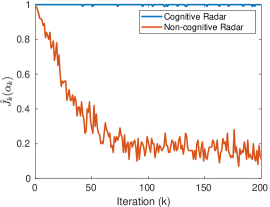
Figure 7: Performance of SPSA Algorithm 3. Given the radar response in beam scheduling amongst 3 targets, we adaptively optimize our probe signal to minimize the probability of Type-II errors in the detector, namely (41). $\hat{J}_{k}(\boldsymbol{\alpha}_{k})$ is the empirical Type-II error probability (42).

VIII Conclusion and Discussion

Cognitive radars adapt their sensing by optimizing their waveform, aperture and beam allocation. The main idea of this paper was to formulate a revealed preference framework (from microeconomics) to detect such constrained utility maximization behavior in radars. As mentioned in the introduction, such methods generalize classical inverse reinforcement learning. The main results of the paper are:
(i) Spectral revealed preferences algorithms to detect if a radar is optimizing its waveform. Our probe input comprises purposeful maneuvers that modulate the spectrum (vector of eigenvalues) of the state noise covariance matrix. The radar responds with an optimized waveform which modulates the spectrum of the observation noise covariance matrix. The spectra of the state and observation noise covariance matrices were used in Afriat’s theorem to detect utility maximization behavior in radar waveforms. A generalization involving nonlinear budgets and the algebraic Riccati equation was obtained. We presented similar methods to detect if a radar is optimizing a utility function when it allocates its beam among multiple targets.
(ii) We then developed stochastic revealed preference tests when either the enemy radar’s response is observed by us in noise, or the enemy radar observes our input in noise. Specifically, we developed a statistical hypothesis test to detect utility maximization behavior by the radar. We gave tight bounds for the Type-I error of the detector.
(iii) Finally we presented an SPSA based stochastic optimization algorithm to adaptively interrogate the enemy radar to detect if it is cognitive. The algorithm minimizes the Type-II detection error subject to constraints on the Type-I error.

Extensions. This paper focused on detecting radars that adapt waveforms to improve tracking. The ideas can be extended to radars which adapt waveforms to improve detection (in clutter and jamming). In this paper, our probing of the enemy radar was performed via purposeful maneuvers by modulating our state covariance matrix $Q$. To extend the result to the latter case, our probing of the enemy radar will involve emitting certain classes of signals and modifying reflected signals so that we can ascertain how the radar changes its waveform to improve detectability.

Finally, the methodology in this paper is an early step in understanding how to design stealthy cognitive radars whose cognitive functionality is difficult to detect by an observer. In future work we will consider how to design a smart radar that acts dumb?. This generalizes the physics based low-probability of intercept (LPI) requirement of radar (which requires low power emission) to the systems-level issue: How should the radar choose its actions in order to avoid detection of its cognition?

References

- [1] S. Haykin, “Cognitive radar,” IEEE Signal Processing Magazine, pp. 30–40, Jan. 2006.
- [2] A. Ng and S. Russell, “Algorithms for inverse reinforcement learning,” in Proc. 17th International Conf. Machine Learning, 2000, pp. 663–670.
- [3] P. Samuelson, “A note on the pure theory of consumer’s behaviour,” Economica, pp. 61–71, 1938.
- [4] S. Afriat, “The construction of utility functions from expenditure data,” International economic review, vol. 8, no. 1, pp. 67–77, 1967.
- [5] ——, Logic of choice and economic theory. Clarendon Press Oxford, 1987.
- [6] W. Diewert, “Afriat’s theorem and some extensions to choice under uncertainty,” The Economic Journal, vol. 122, no. 560, pp. 305–331, 2012.
- [7] H. Varian, “Revealed preference and its applications,” The Economic Journal, vol. 122, no. 560, pp. 332–338, 2012.
- [8] ——, “Non-parametric tests of consumer behaviour,” The Review of Economic Studies, vol. 50, no. 1, pp. 99–110, 1983.
- [9] A. Mas-Colell, M. Whinston, and J. Green, Microeconomic Theory. Oxford, 1995.
- [10] H. Varian, “Revealed preference,” Samuelsonian economics and the twenty-first century, pp. 99–115, 2006.
- [11] ——, “The nonparametric approach to demand analysis,” Econometrica, vol. 50, no. 1, pp. 945–973, 1982.
- [12] ——, “Price discrimination and social welfare,” The American Economic Review, pp. 870–875, 1985.
- [13] F. Forges and E. Minelli, “Afriat’s theorem for general budget sets,” Journal of Economic Theory, vol. 144, no. 1, pp. 135–145, 2009.
- [14] A. Fleissig and G. Whitney, “Testing for the significance of violations of Afrait’s Inequalities,” Journal of Business & Economic Statistics, vol. 23, no. 3, pp. 355–362, 2005.
- [15] B. E. Jones and D. L. Edgerton, “Testing utility maximization with measurement errors in the data,” in Measurement Error: Consequences, Applications and Solutions. Emerald Group Publishing Limited, 2009, pp. 199–236.
- [16] V. Krishnamurthy and W. Hoiles, “Afriat’s test for detecting malicious agents,” IEEE Signal Processing Letters, vol. 19, no. 12, pp. 801–804, 2012.
- [17] A. Aprem and V. Krishnamurthy, “Utility change point detection in online social media: A revealed preference framework,” IEEE Transactions on Signal Processing, vol. 65, no. 7, April 2017.
- [18] S. Haykin, “Cognitive dynamic systems: Radar, control, and radio [point of view],” Proceedings of the IEEE, vol. 100, no. 7, pp. 2095–2103, 2012.
- [19] D. Kershaw and R. Evans, “Optimal waveform design for tracking,” IEEE Transactions on Information Theory, pp. 1536–1551, September 1994.
- [20] V. Krishnamurthy and D. Djonin, “Optimal threshold policies for multivariate POMDPs in radar resource management,” IEEE Transactions on Signal Processing, vol. 57, no. 10, 2009.
- [21] E. K. P. Chong, C. Kreucher, and A. Hero, “Partially observable Markov decision process approximations for adaptive sensing,” Discrete Event Dynamic Systems, vol. 19, no. 3, pp. 377–422, 2009.
- [22] V. Krishnamurthy and D. Djonin, “Structured threshold policies for dynamic sensor scheduling–a partially observed Markov decision process approach,” IEEE Transactions on Signal Processing, vol. 55, no. 10, pp. 4938–4957, Oct. 2007.
- [23] V. Krishnamurthy, Partially Observed Markov Decision Processes. From Filtering to Controlled Sensing. Cambridge University Press, 2016.
- [24] V. Krishnamurthy and M. Rangaswamy, “How to calibrate your adversary’s capabilities? inverse filtering for counter-autonomous systems,” IEEE Transactions on Signal Processing, vol. 67, no. 24, pp. 6511–6525, 2019.
- [25] R. Mattila, I. Lourenço, C. R. Rojas, V. Krishnamurthy, and B. Wahlberg, “Estimating private beliefs of bayesian agents based on observed decisions,” IEEE Control Systems Letters, 2019.
- [26] W. Hoiles, V. Krishnamurthy, and A. Aprem, “PAC algorithms for detecting nash equilibrium play in social networks: From twitter to energy markets,” IEEE Access, vol. 4, pp. 8147–8161, 2016.
- [27] X. R. Li and V. P. Jilkov, “Survey of maneuvering target tracking. part i. dynamic models,” IEEE Transactions on Aerospace and Electronic Systems, vol. 39, no. 4, pp. 1333–1364, 2003.
- [28] Y. Bar-Shalom, X. R. Li, and T. Kirubarajan, Estimation with applications to tracking and navigation. New York: John Wiley, 2008.
- [29] H. V. Trees, Detection, Estimation and Modulation Theory. John Wiley & Sons, 1968.
- [30] B. D. O. Anderson and J. B. Moore, Optimal filtering. Englewood Cliffs, New Jersey: Prentice Hall, 1979.
- [31] J. Spall, Introduction to Stochastic Search and Optimization. Wiley, 2003.
- [32] H. J. Kushner and G. Yin, Stochastic Approximation Algorithms and Recursive Algorithms and Applications, 2nd ed. Springer-Verlag, 2003.
- [33] M. Frankel, “The production function in allocation and growth: a synthesis,” The American Economic Review, vol. 52, no. 5, pp. 996–1022, 1962.
- [34] A. S. Goldberger, “The interpretation and estimation of cobb-douglas functions,” Econometrica: Journal of the Econometric Society, pp. 464–472, 1968.