WLS-ENO Remap: Superconvergent and Non-Oscillatory
Weighted Least Squares Data Transfer on Surfaces

Abstract

Data remap between non-matching meshes is a critical step in multiphysics coupling using a partitioned approach. The data fields being transferred often have jumps in function values or derivatives. It is important but very challenging to avoid spurious oscillations (a.k.a. the Gibbs Phenomenon) near discontinuities and at the same time to achieve high-order accuracy away from discontinuities. In this work, we introduce a new approach, called WLS-ENOR, or Weighted-Least-Squares-based Essentially Non-Oscillatory Remap, to address this challenge. Based on the WLS-ENO reconstruction technique proposed by Liu and Jiao (J. Comput. Phys. vol 314, pp 749–773, 2016), WLS-ENOR differs from WLS-ENO and other WENO schemes in that it resolves not only the $\mathcal{O}(1)$ oscillations due to $C^{0}$ discontinuities, but also the accumulated effect of $\mathcal{O}(h)$ oscillations due to $C^{1}$ discontinuities. To this end, WLS-ENOR introduces a robust detector of discontinuities and a new weighting scheme for WLS-ENO near discontinuities. We also optimize the weights at smooth regions to achieve superconvergence. As a result, WLS-ENOR is more than fifth-order accurate and highly conservative in smooth regions, while being non-oscillatory and minimally diffusive near discontinuities. We also compare WLS-ENOR with some commonly used methods based on $L^{2}$ projection, moving least squares, and radial basis functions.

1 Introduction

In multiphysics applications with a partitioned approach, data often must be mapped between different meshes [63]. This problem is often referred to as data transfer or remap, and the two meshes are often referred to as the source (or donor) and target (or donee) mesh, respectively. In many of these applications, the data approximate a piecewise smooth function, where discontinuities (or jumps) may be present in the solutions, for example, due to shocks in high-speed fluids or multi-material solids. In addition, nowadays the physics models are often discretized with third or higher-order methods, such as $hp$ finite elements [61], spectral elements [68], discontinuous Galerkin [15], etc. The combination of the discontinuities and high-order methods lead to a fundamental challenge for remap: high-order interpolations (such as splines [19]) or least squares (such as moving least squares (MLS) [103]) are prone to spurious oscillations near discontinuities [26, 46]. In particular, $C^{0}$ discontinuities, a.k.a. (simple) jumps, often lead to $\mathcal{O}(1)$ oscillations (overshoots or undershoots), analogous to the Gibbs-Wilbraham phenomenon in Fourier transformation [32, 105, 46]. In addition, $C^{1}$ discontinuities, a.k.a. derivative jumps, can lead to $\mathcal{O}(h)$ oscillations, which may accumulate in repeated transfer or in time-dependent settings. Even some second and lower order methods, such as $L^{2}$ projection [49] and radial basis function (RBF) interpolation [4, 25, 82] can suffer from such oscillations [26, 27]. Among the existing methods, nearest-point or linear interpolation have no oscillation, but they do not deliver sufficient accuracy and are excessively diffusive in repeated transfer. The objective of this work is to propose a new data-transfer method that is at least third-order accurate for smooth functions, is non-oscillatory at discontinuities, and is as non-diffusive as possible.

Resolution of the Gibbs phenomenon or similar oscillations is an important and challenging subject in numerical analysis and computational physics. There have been various methods developed for it in various contexts; see e.g. [35]. Among these, the most closely related ones are probably the so-called reconstruction methods, such as flux reconstructions based on WENO [72, 92] and their variants in finite volume methods. The connection is even closer in the context of hyperbolic conservation laws, in that they are time dependent. However, in the context of hyperbolic PDEs, it typically suffices for the reconstruction to resolve only simple jumps, because small oscillations due to $C^{1}$ discontinuities can be effectively controlled by the numerical diffusion in flux limiters [69] and TVD time-integration schemes [36]. In contrast, a general remap technique must be stable without assuming numerical diffusion in the physics models. Hence, it is important to control the oscillations due to both simple and derivative jumps in remap. This property makes remap significantly more challenging.

In this work, we introduce a new method, called WLS-ENOR, or Weighted-Least-Squares-based Essentially Non-Oscillatory Remap. WLS-ENOR is based on the WLS-ENO scheme proposed by Liu and Jiao [71] for the finite volume methods. The original WLS-ENO controls oscillations by adapting the weights in a weighted-least-squares (WLS) approximation, where the weights are approximately based on the inverse of a non-smoothness indicator. However, the indicator in WLS-ENO only considers simple jumps. WLS-ENOR introduces a novel technique to detect both simple and derivative jumps by introducing two novel indicators and a new dual-thresholding strategy. We then apply WLS-ENO near the detected singularities by using a new weighting scheme to take into account $C^{1}$ discontinuities. We also optimize WLS-ENOR for smooth functions to achieve superconvergence. As a result, WLS-ENOR is more than fifth-order accurate for smooth functions, non-oscillatory and minimally diffusive near $C^{0}$ and $C^{1}$ discontinuities, and is highly conservative in repeated transfers. We compare WLS-ENOR with some commonly used methods, including linear interpolation, RBF interpolation [4], $L^{2}$ projection [49], and modified moving least squares (MMLS) [54, 94], and show that WLS-ENOR is more accurate, stable, and less diffusive in almost all cases. The presentation and results in this work focus on spherical geometries in earth and climate modeling. However, the methodology also applies to other smooth surfaces.

The remainder of this paper is organized as follows. In Section 2, we review some preliminaries on remap and reconstruction methods and the Gibbs phenomenon at discontinuities. In Section 3, we describe WLS fittings for smooth functions that exhibit superconvergence. In Section 4, we describe the detection of discontinuities in data remapping and a new weighting scheme for WLS-ENO for discontinuities. In Section 5, we compare WLS-ENOR with other methods for transferring both smooth and discontinuous functions. Finally, Section 6 concludes the paper with a discussion on future research directions.

2 Preliminaries and related work

In this section, we review some methods for remap and reconstruction, especially the high-order methods based on weighted-least-squares (WLS). In addition, we review some concepts and methods related to discontinuities, including Gibbs phenomena and WLS-ENO.

2.1 Remap and reconstruction methods

The remap problem has been studied extensively in the past few decades. Several software packages have been developed over the past two decades. These include those developed for climate and earth modeling (such as those in Earth System Modeling Framework (ESMF) [42], Community Earth System Model (CESM) [45] and the next-generation Energy Exascale Earth System Model (E3SM), including SCRIP [55], Model Coupling Toolkit (MCT) [66], OASIS [17], Tempest Remap [99, 98], etc.), fluid-structure interaction or heat transfer (such as MpCCI [56] and preCICE [11]), and general-purpose remap software (such as PANG [28] and Data Transfer Kit (DTK) [93, 94]). We first review the methodology behind some of these packages, with a focus on node-to-node transfer, and then review some closely related methods for high-order reconstruction.

2.1.1 Low-order nonconservative and conservative remap

In 1990s and 2000s, data-transfer methods primarily on only first- or second-order accuracy, because the prevailing numerical discretization methods in engineering (including finite volume methods and linear finite element methods) only had low-order accuracy. One of the most primitive data-transfer methods is piecewise interpolation. This approach is particularly convenient if the source mesh has an associated finite-element function space, in that one could use the same function space for interpolation. In this case, we refer to the approach as consistent interpolation. If the basis functions are linear (with simplicial elements) or bilinear (with quadrilateral elements), the interpolation is second order. In a finite-volume method and scatter-data interpolation, the nearest-point interpolation is sometimes used, which is only first-order accurate. If the basis functions are not known, some interpolation (and more precisely, quasi-interpolation [19]) methods can use some alternative basis functions, such as thin-plate splines [38] or other RBF [4, 11, 25, 82].

The major disadvantage of low-order interpolation is its high diffusiveness in repeated transfer; see e.g. [18]. To overcome this, one approach is to enforce conservation, so that the integrals over the source and target meshes are equal. Examples of lower-order conservative methods include the first- and second-order conservative remap (such as those in [14, 37, 28, 55]), common-refinement-based $L^{2}$ projection [49], etc. A commonality of these methods is that they all require computing some integrals of the function defined on the source mesh over some control volumes of each target node (or cell), and the numerical integration is computed over the intersections of the elements (or cells) of the source and target meshes. The collection of these intersections forms the common refinement [49] or supermesh [23, 22], whose computations require some sophisticated computational-geometry algorithm for efficiency and for robustness in the presence of truncation and rounding errors [50, 51]. We also note that some low-order constrained interpolation and conservative remap methods have been developed in the context of Arbitrary Lagrangian-Eulerian (ALE) methods, such as [5, 76].

2.1.2 High-order remap methods

Due to the increasing use of high-order discretization methods, more recent development of data-transfer methods had focused on third and higher order methods. If the source mesh uses a high-order finite element or spectral element method, one can apply consistent interpolation to achieve high-order accuracy. Such an approach may be implemented with a discretization library, such as MOAB [96, 75]. More generally, a remap method can be independent of the discretization methods. In this context, the method may be nonconservative or conservative. Examples of the former include modified moving least square (MMLS) [54, 94], etc. An example of the latter is the conservative remap in Tempest Remap [99, 98] and conservative interpolation [1]. Note that high-order nonconservative remap methods tend to be significantly less diffusive in repeated transfer than low-order nonconservative methods, even though conservation is not enforced explicitly; see e.g. [94]. However, because high-order methods are more prone to oscillations, special attention is needed to preserve positivity and convexity [99, 98].

2.1.3 High-order reconstructions

The remap methods, especially the nonconservative ones, are closely related to the reconstruction problem, i.e., to reconstruct a piecewise smooth function or its approximations at some discrete points on a mesh given some known qualities at discrete points or cells on the same mesh. The primary difference between remap and reconstruction is that the former involves two meshes while the latter typically involves only a single mesh. Hence, remap is in general more complicated from a combinatorial point of view. From a numerical point of view, conservation in remap is also more complicated than in reconstruction. However, nonconservative high-order remap and reconstruction share many similarities. In particular, the techniques used in high-order remap, such as spline interpolation [19], moving least square (MLS) [64], and variants of MLS (known as MMLS) with regularization [54, 94], etc., originated from high-order reconstruction.

The remap method in this work utilizes two high-order reconstruction techniques, known as CMF (Continuous Moving Frames) and WALF (Weighted Average of Least-squares Fittings) [52], both of which are based on weighted least squares (WLS). These techniques were first proposed for reconstructing surfaces and later adapted to reconstruct functions on surfaces [81]. CMF shares some similarities with some variant of MMLS (such as that in [94]), in that CMF constructs a least-squares fitting at each reconstruction point and it achieves accuracy and stability through some local adaptivity (instead of the global construction of the original MLS for smoothness [65]). However, CMF differs from MLS in terms of the choice of the coordinate systems, stencils, and weighting schemes. WALF constructs a least-squares fitting at each node of a mesh using CMF and then blend the fittings taking a weighted average using piecewise linear or bilinear basis functions within each element (such as a triangle or quadrilateral). In general, CMF is more accurate than WALF. For meshing applications, WALF tends to be more efficient when many points need to be evaluated within a single element. For remap in multiphysics applications, however, a transfer operator can be built in a preprocessing step and be reused in repeated transfers. Hence, In this work, we use CMF as the basis for remapping smooth regions. From the mathematical point of view, the major challenge is to overcome the potential oscillations (a.k.a. the Gibbs phenomenon) associated with CMF, for which we will leverage WALF to detect singularities.

2.2 Gibbs phenomena at $C^{0}$ and $C^{1}$ discontinuities

It is well known that discontinuities require special attentions in numerical approximations. The most studied type is the $C^{0}$ discontinuities, also known as edges [95], (simple) jump discontinuities [13, 40], faults (or vertical faults) [7, 20], etc. These discontinuities are the most prominent because they tend to lead to $\mathcal{O}(1)$ oscillations (or “ringing”), which do not vanish under mesh refinement. These oscillations were first analyzed by Wilbraham in 1848 [105], about 50 years before the famous analysis of the overshoots in Fourier series for saw-tooth functions by Gibbs in 1899 [32] in response to an observation by Michelson in 1898 [77]. For this reason, such oscillations are properly referred to as the Gibbs-Wilbraham phenomenon [40], or more commonly as the Gibbs phenomenon. Besides occurring in Fourier series, the $\mathcal{O}(1)$ oscillations also occur in interpolation or approximation using cubic splines [83, 112], orthogonal polynomials [35], RBF [26, 58], least squares [27], wavelets [62, 89], $L^{2}$ projection [49], etc. Some tight constant factors can be established in 1D for some of these problems. However, for least-squares-based approximations in 2D and higher dimensions, it is impractical to establish such a precise bound of the oscillations. Instead, we focus on the asymptotic effect of discontinuities, which is easy to understand from the Taylor series expansion and is sufficient for developing robust techniques to detect and resolve them in this work.

Consider a piecewise smooth function $f(\boldsymbol{x}):\mathbb{R}^{d}\rightarrow\mathbb{R}$. The $d$-dimensional Taylor series of $f$ about a point $\boldsymbol{x}_{0}$ is given by

$$f(\boldsymbol{x}_{0}+\boldsymbol{h}) =\sum_{k=0}^{p}\frac{1}{k!}\partial_{\hat{\boldsymbol{h}}}^{k}f(\boldsymbol{x}_{0})\left\|\boldsymbol{h}\right\|_{2}^{k}+\frac{\partial_{\hat{\boldsymbol{h}}}^{p+1}f(\boldsymbol{x}_{0}+\boldsymbol{\epsilon})}{(p+1)!}\|\boldsymbol{h}\|_{2}^{p+1},$$ (1)

where $\partial_{\hat{\boldsymbol{h}}}^{k}$ denotes the $k$th directional derivative along the direction $\hat{\boldsymbol{h}}=\boldsymbol{h}/\left\|\boldsymbol{h}\right\|_{2}$, and $\|\boldsymbol{\epsilon}\|\leq\|\boldsymbol{h}\|$; see, e.g., [44] for a proof. The summation term in (1) defines the degree-$p$ Taylor polynomial $T_{p}(\boldsymbol{x})$ at $\boldsymbol{x}_{0}$. The last term in (1) is the remainder $r(\boldsymbol{x})$, which corresponds to the residual of the approximation $f(\boldsymbol{x})$ by $T_{p}(\boldsymbol{x})$. If $f$ is continuously differentiable to at least $p$th order, the residual $r(\boldsymbol{x})$ is $\mathcal{O}(\|\boldsymbol{h}\|_{2}^{p+1})$, i.e.,

$$\left|r(\boldsymbol{x})\right|=\left|f(\boldsymbol{x})-T_{p}(\boldsymbol{x})\right|=\mathcal{O}(\|\boldsymbol{h}\|_{2}^{p+1}).$$ (2)

However, if $f$ has a $C^{q}$ discontinuity in the direction $\hat{\boldsymbol{h}}$ at $\boldsymbol{x}_{0}+\boldsymbol{\epsilon}$, i.e., $\partial_{\hat{\boldsymbol{h}}}^{q}f$ has a jump at $\boldsymbol{x}_{0}+\boldsymbol{\epsilon}$, then $\partial_{\hat{\boldsymbol{h}}}^{p+1}f$ is unbounded. As a result, the approximation of $f(\boldsymbol{x})$ by $T_{p}(\boldsymbol{x})$ in general are expected to lead to overshoots or undershoots (or oscillations) of $\mathcal{O}(\|\boldsymbol{h}\|_{2}^{p})$ or larger. Note that even if $f$ is approximated by non-polynomials, this argument based on Taylor series also applies with a simple application of triangle inequality. In particular, let $g(\boldsymbol{x})$ be a smooth approximation of $f$ and let $\tilde{T}_{p}$ denote the degree-$p$ Taylor polynomial of $g(\boldsymbol{x})$ at $\boldsymbol{x}_{0}$. Then,

$$\left|f(\boldsymbol{x})-g(\boldsymbol{x})\right|\leq\left|r(\boldsymbol{x})\right|+\left|g(\boldsymbol{x})-\tilde{T}_{p}(\boldsymbol{x})\right|,$$ (3)

where the second term is $\mathcal{O}(\|\boldsymbol{h}\|_{2}^{p+1})$ under the smoothness assumption of $g$, but the first term is $\mathcal{O}(\|\boldsymbol{h}\|_{2}^{p})$ or larger and it dominates the overall error. Hence, for $C^{0}$ discontinuities, we can expect to observe $\mathcal{O}(1)$ oscillations, even when using linear approximations, as in $L^{2}$ projection using linear polynomials.

From the Taylor series expansions, it is easy to see that overshoots can occur not only at $C^{0}$ discontinuities but also at $C^{1}$ and even $C^{2}$ discontinuities. In general, the oscillations due to $C^{1}$ discontinuities are expected to be $\mathcal{O}(h)$. Theoretically, these oscillations should vanish as $h$ tends to $0$, so they are often ignored. However, its treatment has drawn some attention recently, and it is often referred to as derivative jump discontinuities [13] or oblique (or gradient) faults [7, 20]. In the context of data transfer in multiphysics coupling, it is important to resolve the $\mathcal{O}(h)$ oscillations at $C^{1}$ discontinuities, because they may accumulate over time and lead to $\mathcal{O}(1)$ oscillations and even instabilities. Although these $\mathcal{O}(h)$ oscillations may be controlled by numerical diffusion in some numerical schemes, such as the flux limiters and TVD time integration schemes in FVM for hyperbolic conservation laws, for generality, it is desirable for the data-transfer method to be stable without relying on numerical diffusion in physics models. In addition, controlling $\mathcal{O}(h)$ oscillations also helps safeguarding the accumulation of the $\mathcal{O}(h^{2})$ oscillations near $C^{2}$ discontinuities.

2.3 Resolution of Gibbs oscillations

2.3.1 Resolution of oscillations in 1D

Because the mathematical analysis of the Gibbs phenomenon in the literature primarily focused on 1D reconstructions, the overwhelming majority of the resolution techniques were also for 1D problems. We briefly mention two classes of classical techniques in 1D. The first class is filtering and mollification, which recovers the piecewise solutions in Fourier spaces and in physical spaces, respectively. Examples of the former include Fejer averaging, Lanczos-like filtering, Vandeven and Daubechies filters, etc., which are specific to Fourier expansions; see e.g. [114] and [46, Chapter 2] for some surveys. Examples of the latter include spectral mollifiers based on Gegenbauer polynomials in [35, 60, 90] and adaptive mollifiers in [95]. The fundamental idea of adaptive mollifiers is to detect the edges [29, 30] and then apply spectral (or other) mollifiers locally. Similar ideas have been applied for approximating piecewise smooth functions in 1D using splines and moving least squares in [70].

The second class is the Godunov and ENO-type methods. Examples include the original Godunov’s method [33], Van Leer’s MUSCL scheme [100], Colella and Woodward’s piecewise parabolic method (PPM) [16], Harten’s subcell-resolution method [39], and some WENO reconstructions for FVM [72, 47, 91]. These methods were initially developed for the finite volume methods (FVM) for hyperbolic problems, and they typically involve reconstructing piecewise smooth functions from cell averages. Among these techniques, the ENO and WENO techniques are the most general, and their key ideas lie at the approximation level, where a nonlinear adaptive procedure is used to automatically choose the locally smoothest stencil, hence avoiding crossing discontinuities in the interpolation process as much as possible. This basic idea can be generalized to reconstructing nodal values, such as in the so-called WENO interpolation in finite difference methods [92]. Similar to mollifiers, the WENO schemes may be applied globally without explicitly identifying the discontinuities, or be applied adaptively by coupling with some edge-detection techniques [80].

2.3.2 Resolution of oscillations in higher dimensions

The two broad classes of 1D techniques may be applied to structured meshes in a dimension-by-dimension fashion. For example, in climate modeling, Lauritzen and Nair [67] developed monotonicity-preserving filters on latitude–longitude and cubed-sphere grids by adapting those developed by Zerroukat et al. using monotonic parabola [109] or parabolic spline method (PSM) [110]. However, when generalizing the techniques to unstructured meshes or scattered data, most of the techniques in 1D or for structured meshes encounter significant technical difficulties. However, some of the basic ideas can still be preserved on higher dimensions. Hence, we also broadly categorize the methods into two classes.

The filtering techniques in 2D and higher dimensions typically reply on post-processing to resolve oscillations. This requires detecting the discontinuities and then adapt the kernels (i.e., basis functions) accordingly. Various techniques have been developed in the literature to detect discontinuities. The detection of $C^{0}$ discontinuities is often referred to as edge detection [3, 12, 31, 78, 84, 101, 113] or troubled-cell detection [80, 108], and it has many applications in signal and image processing, data compression, shock capturing in CFD, etc. These techniques typically use some indicators for the jump and then compare the indicator against some thresholds. Similarly, detecting $C^{1}$ discontinuities requires an indicator of the derivative jump followed by some thresholding. The indicators are often motivated by finite differences (such as in [7, 13, 20]) or Taylor series expansions (such as in the polynomial annihilation edge detection in [2, 3, 87]). In [59], Jung et al. detected discontinuities by taking advantage of the instabilities of the expansion coefficients of multiquadric RBF at local jumps. Romani et al. [84] developed some variants of the approach using variably scaled kernels (VSK) [6] and Wendland’s $C^{2}$ RBF [102]. In terms of thresholding, they are often based on some statistical analysis (i.e., outlier detection) [24] or based on some double (or hysteresis) thresholding [12]. After the discontinuities have been detected, various reconstruction strategies have been used in practice. For reconstructions over structured grids, such as in image processing, it is relatively straightforward to adapt some limiters used in hyperbolic conservation laws to resolve discontinuities in a dimension-by-dimension fashion, such as in [3, 31]. However, such an approach does not generalize to unstructured meshes easily. For unstructured meshes or scattered data points, Rossini [85] proposed to use VSK to resolve discontinuities, but it required the exact location of discontinuities in order to shift the radial functions.

In terms of Godunov and ENO-type methods, the generalization of the low-order methods tends to be straightforward within FVM. However, for the high-order ENO and WENO schemes, the generalization to unstructured meshes is challenging. In [43], Hu and Shu proposed a WENO scheme on triangular meshes, and it was further extended to tetrahedral meshes by Zhang and Shu in [111]. However, some point distributions may lead to negative weights and in turn lead to potential instability. Shi, Hu and Shu [88] proposed a technique to mitigate the issue, but the method had limited success due to large condition numbers of the local linear systems. In [107], Xu et al. proposed a hierarchical reconstruction technique for discontinuous Galerkin and finite volume methods on triangular meshes, and Luo et al. [74] extended the ideas to tetrahedral meshes and developed the so-called hierarchical WENO (or HWENO). In [73], Liu and Zhang proposed a hybrid of two different reconstruction strategies to improve stability of WENO reconstruction. In [71], Liu and Jiao proposed WLS-ENO, which adapts the weights in a weighted least squares formulation instead of taking a convex combination of interpolations. WLS-ENO overcomes the stability issues associated negative weights, and it was shown to be robust in FVM and is easy to implement.

The resolution technique proposed in this work may be considered as a hybrid of adaptive mollification and ENO-type method, in that we detect $C^{0}$ and $C^{1}$ discontinuities in high-order CMF and then apply quadratic WLS-ENO as mollifier (or filters in the physical space) near discontinuities. Our detection technique is different from others in that it introduces two novel discontinuity indicators and a novel dual thresholding strategy to detect discontinuities. The indicators use the observation that WALF tends to be more prone to oscillations than CMF near discontinuities, so that we can detect and resolve discontinuities before oscillations manifest themselves in CMF. In addition, we will introduce a new weighting scheme for WLS-ENO based on one of the new discontinuity indicators.

3 Superconvergent weighted least squares (WLS)

In this section, we describe WLS remap for smooth functions on surface.

3.1 WLS with Cartesian coordinates

We first derive WLS in Cartesian coordinates using Taylor series. Consider a function $f(\boldsymbol{u}):\mathbb{R}^{2}\rightarrow\mathbb{R}$ at a given point $\boldsymbol{u}_{0}=\left[0,0\right]^{T}$, and assume its value is known at a sample of $m$ points $\boldsymbol{u}_{i}$ near $\boldsymbol{u}_{0}$, where $1\leq i\leq m$. We refer to these points as the stencil for WLS. Suppose $f$ is continuously differentiable to $(p+1)$st order for some $p>1$. We approximate $f(\boldsymbol{u})$ to ($p+1$)st order accuracy about $\boldsymbol{u}_{0}$ as

$$f(\boldsymbol{u})=\sum_{q=0}^{p}\sum_{j,k\geq 0}^{j+k=q}c_{jk}u^{j}v^{k}+\mathcal{O}\left(\|\boldsymbol{u}\|^{p+1}\right),$$ (4)

which is an alternative form of that in (1), where $c_{jk}=\dfrac{1}{j!k!}\dfrac{\partial^{j+k}}{\partial u^{j}\partial v^{k}}f(\boldsymbol{0})$. Supper there are $n$ coefficients, i.e., $n=(p+1)(p+2)/2$, and assume $m\geq n$. Let $f_{i}$ denote $f(\boldsymbol{u}_{i})$. We then obtain a system of $m$ equations

$$\sum_{q=0}^{p}\sum_{j,k\geq 0}^{j+k=q}c_{jk}u_{i}^{j}v_{i}^{k}\approx f_{i}$$ (5)

for $1\leq i\leq m$. The equation can be written in matrix form as $\boldsymbol{A}\boldsymbol{x}\approx\boldsymbol{b}$, where $\boldsymbol{A}\in\mathbb{R}^{m\times n}$ is an generalized Vandermonde matrix, $\boldsymbol{x}\in\mathbb{R}^{n}$ is composed of $c_{jk}$, and $\boldsymbol{b}\in\mathbb{R}^{m}$ is composed of $f_{i}$.

The generalized Vandermonde system from (5) is rectangular, and we solve it by minimizing a weighted norm of the residual vector $\boldsymbol{r}=\boldsymbol{b}-\boldsymbol{A}\boldsymbol{x}$, i.e.,

$$\min_{\boldsymbol{x}}\|\boldsymbol{r}\|_{\boldsymbol{W}}\equiv\min_{\boldsymbol{x}}\|\boldsymbol{W}(\boldsymbol{A}\boldsymbol{x}-\boldsymbol{b})\|_{2},$$ (6)

where $\boldsymbol{W}=\mbox{diag}\{\omega_{1},\omega_{2},\dots,\omega_{m}\}$ is diagonal. The weighting matrix $\boldsymbol{W}$ plays a fundamental role in $\boldsymbol{W}$, in that each diagonal entry $w_{i}$ in $\boldsymbol{W}$ assigns a weight to each row in the generalized Vandermonde system. If both $\boldsymbol{A}$ and $\boldsymbol{W}$ are both nonsingular, then $\boldsymbol{W}$ has no effect on the solution. However, if $m\neq n$ or $\boldsymbol{A}$ is singular, then a different $\boldsymbol{W}$ leads to a different solution; we will address the choice of the weights shortly. Given $\boldsymbol{W}$, we further scale the columns of $\boldsymbol{W}\boldsymbol{A}$ with a diagonal matrix $\boldsymbol{T}$, so that the condition number of the rescaled Vandermonde matrix $\tilde{\boldsymbol{A}}=\boldsymbol{W}\boldsymbol{A}\boldsymbol{T}$ is improved. This process is known as column equilibration [34, p. 265]. Then, WLS reduces to the least squares problem

$$\boldsymbol{W}\boldsymbol{A}\boldsymbol{T}\boldsymbol{y}\approx\boldsymbol{W}\boldsymbol{b}.$$ (7)

The coefficients in $c_{ij}$ are then given by $\boldsymbol{x}=\boldsymbol{T}\boldsymbol{y}$.

We give two important algorithmic details. First, we solve (7) using truncated QR factorization with column pivoting (QRCP) [34]. The QRCP is

$$\tilde{\boldsymbol{A}}\boldsymbol{P}=\boldsymbol{Q}\boldsymbol{R},$$ (8)

where $\boldsymbol{Q}$ is $m\times n$ with orthonormal column vectors, $\boldsymbol{R}$ is an $n\times n$ upper-triangular matrix, $\boldsymbol{P}$ is a permutation matrix, and the diagonal entries in $\boldsymbol{R}$ are in descending order. Second, we control the condition number of $\tilde{\boldsymbol{A}}$ to avoid numerical instabilities. To this end, we estimate the 1-norm condition number of $\boldsymbol{R}$ [41]. If the condition number is large, then we first try to enlarge the stencils and then incrementally drop the right-most highest-degree terms in $\tilde{\boldsymbol{A}}\boldsymbol{P}$ if the stencils cannot be enlarged further. These strategies add more rows to, and remove columns from, the Vandermonde systems, respectively, both of which reduce the condition number of $\tilde{\boldsymbol{A}}$ and in turn ensure the stability of WLS.

3.2 WLS on discrete surfaces

When applying WLS on surfaces, we use the same construction as in Continuous Moving Frames (CMF) for high-order surface reconstruction [52]. We adapt CMF to remap between discrete surfaces composed of triangles and quadrilaterals. In the following, we will use WLS and CMF interchangeable, unless otherwise noted.

Given a node $\boldsymbol{x}_{0}$ on a target mesh, we first construct a local $uv$ coordinate frame as follows. Let $\boldsymbol{m}_{0}$ denote an approximate normal at $\boldsymbol{x}_{0}$, which can be first-order estimation by averaging face normals or be computed from the analytical surface (such as a sphere in earth modeling). Let $\boldsymbol{t}_{1}$ and $\boldsymbol{t}_{2}$ be an orthonormal basis of approximate tangent plan orthogonal to $\boldsymbol{m}_{0}$, which we obtain using Gram-Schmidt orthogonalization. The local $uv$ coordinate frame is then centered at $\boldsymbol{x}_{0}$ with axes $\boldsymbol{t}_{1}$ and $\boldsymbol{t}_{2}$.

The construction of stencils requires some special attention in remap. Unlike reconstruction, the stencil for a target node is composed of nodes on the source mesh. To build the stencil for a target node $\boldsymbol{x}_{0}$, we first locate the triangle or quadrilateral $\tau$ on the source mesh that contains $\boldsymbol{x}_{0}$, and then use the union of the $k$-ring neighborhood of each node of $\tau$ on the source mesh. The specific choice of $k$ depends on the degree of the polynomial and the specific weighting scheme, as we will describe in Section 3.3.

We note some key difference between our WLS remap and MMLS in DTK when applied to surfaces. First, our approach uses 2D Taylor series within local $uv$ coordinates in a tangent space, whereas DTK uses the global $xyz$ coordinate system. Note that for degree-$p$ polynomials, the number of coefficients grows quadratically in 2D but cubically in 3D. Hence, it is more efficient to use higher-degree (such as quartic) fittings with CMF to achieve higher accuracy than DTK. Second, DTK is purely mesh-less and it finds stencils by using $k$ nearest neighbors (a.k.a. KNN), which requires logarithmic-time complexity on average to determine the stencils. In contrast, our approach uses a mesh-based algorithm to compute the stencils by taking advantage of locality [48], so the amortized cost to determine the stencil of a node is constant.

3.3 Optimizing weights for remap

As shown in [53] and [81], if the condition number of the rescaled Vandermonde system $\tilde{\boldsymbol{A}}$ is bounded, then the function values of a smooth function $f:\Gamma\rightarrow\mathbb{R}$ can be reconstructed to $\mathcal{O}(h^{p+1})$ on a discrete surface $\Gamma$, where $h$ is proportional to the “radius” of the stencil. Furthermore, if the stencils are (nearly) symmetric about the origin of the local coordinate system, the reconstruction can superconverge at $\mathcal{O}(h^{p+2})$ for even-degree $p$ due to error cancellation [53, 52], analogous to the error cancellation in centered differences. When using CMF for remap, however, the near-symmetry assumption is in general violated, because a target node may lie anywhere within an element of a source mesh. Hence, it is impractical to achieve $\mathcal{O}(h^{p+2})$ superconvergence. However, with proper choice of stencils and weighting schemes, we can achieve $\mathcal{O}(h^{p+1+s})$ convergence for some $0<s\leq 1$ for even $p$. To maximize this rate, we observe two key criteria for the weights: asymptotic rates and smoothness of the weights.

In [53], Jiao and Zha proposed to use weights that are approximately inversely proportional to the square root of the residual term associated with each node, i.e.,

$$\omega_{j}^{\text{ID}}=\gamma_{j}^{+}\left(\sqrt{r_{j}^{2}+\epsilon_{\text{ID}}}\right)^{-p/2},$$ (9)

where $r_{j}=\left\|\boldsymbol{u}_{j}\right\|$, $p$ is the degree of the WLS, $\epsilon$ is a safeguard against division by zero, and

$$\gamma_{i}^{+}=\max\{0,\boldsymbol{m}_{j}^{T}\boldsymbol{m}_{0}\}$$ (10)

is a safeguard against “short circuiting” for coarse meshes. We refer to (9) as the inverse-distance-based weights. These weights perform well with nearly symmetric stencils. However, they are not ideal for remap, because it has a large gradient near $\boldsymbol{x}_{0}$, especially if $\epsilon_{\text{ID}}$ is small. Therefore, if the nodes closest to $\boldsymbol{x}_{0}$ are highly asymmetric, which tend to be the case in remap, then there is no error cancellation for these nodes. To overcome this issue, it is desirable for the weights to be smoother about the origin, or more precisely, the first, second, and even higher-order derivatives of the weight should $0$ at the origin. This analysis led us to the choice of a new weighting scheme, or scaled Buhmann’s function,

$$\omega_{j}^{\text{SB}}=\gamma_{j}^{+}\phi(r_{j}/\rho),$$ (11)

where $\gamma_{j}^{+}$ and $r_{j}$ are the same as those in (9), $\rho$ is the cut-off radius, and

$$\phi(r)=\begin{cases}\frac{112}{45}r^{9/2}+\frac{16}{3}r^{7/2}-7r^{4}-\frac{14}{15}r^{2}+1/9&\text{if }0\leq r\leq 1\\ 0&\text{if }r>1\end{cases}.$$ (12)

The function $\phi(r)$ is a $C^{3}$ function due to Buhmann [8], who introduced it as a compactly supported RBF by generalizing the polynomial radial functions due to Wu [106] and Wendland [102]. Besides compactness and smoothness, these radial functions are “positive definite,” which is a desirable property for RBF [9, 10] but is irrelevant in our context. In Section 5.1.1, we will compare our proposed scaled Buhmann weights versus other weighting functions.

In (11), the key question is how to choose the cut-off radius $\rho$. For robustness, this radius must be large enough to allow sufficient number of nonzero weights in the generalized Vandermonde system. As in [53], we require the number of points in the stencil to be at least 1.5 times of that of the number of coefficients in the Taylor polynomial. Let $R=r_{k}$, where $k=\left\lceil 0.75(p+1)(p+2)\right\rceil$. We define $\rho=\sigma R$ for some $\sigma>1$ and then choose $\sigma$ to minimize the remap errors via numerical optimization, as we will detail in Section 5.1.1. Through numerical optimization, we obtain $\sigma=2.0$, 1.6 and $1.4$ for degree-2, 4, and 6 WLS, respectively. Figure 1 shows the example shapes of inverse-distance-based and scaled Buhmann weights on a uniform 2D mesh for degree-2, 4, and 6 WLS. For inverse-distance weights, we used $\epsilon_{\text{ID}}=0.01\bar{h}^{2}$, where $\bar{h}$ denotes the average edge length. It can be seen that due to its $C^{3}$ continuity, Buhmann’s function is much smoother at $r=0$. In addition, the different cut-off radii led to different asymptotic behaviors of the scale Buhmann weights at the tails, similar to those of the inverse-distance-based weights.

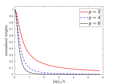
(a) Weights based on inverse-distance.

(b) Weights based on Buhmann’s function

Figure 1: Example shapes of inverse-distance-based and scaled Bushman weights.

In terms of implementation, to select the candidate nodes in the stencils for a target node $\boldsymbol{x}_{0}$, we start with the union of $\lfloor 1.5p\rfloor/2$-rings of the nodes of the source element that contains a given target node. If there are less than $0.75(p+1)(p+2)$ points in the stencil, we enlarge the ring size in 0.5 increments as defined in [52]. This adaptive computation of rings requires a proper mesh data structure to achieve constant-time per node, for which we use an array-based half-edge data structure [21]. In addition, for efficiency, we construct the transfer operator in the form of a sparse matrix, of which each row corresponds to a node in the target mesh. After obtaining this operators, the remap involves only a matrix-vector multiplication.

4 Detection and resolution of $C^{0}$ and $C^{1}$ discontinuities

Like other high-order methods, WLS with scaled Buhmann weights may suffer from Gibbs phenomena near discontinuities. In this section, we extend the WLS-ENO approach to remap. For accuracy and efficiency, our approach first detects the discontinuous regions and then applies WLS-ENO to the detected discontinuities. To this end, we introduce a robust detector of discontinuities and a new weighting scheme for WLS-ENO.

4.1 Detection of discontinuities

We first describe a robust technique to detect discontinuities in the context of remap. Our approach is composed of four steps. First, we compute element-based discontinuity indicators on the source mesh. Second, we convert these indicators to node-based indicators on the source mesh. Third, we obtain node-based discontinuity markers on the source mesh using a novel dual-thresholding strategy. Finally, we transfer the nodal markers to the target mesh. In the following, we describe the four steps separately, including their derivations.

4.1.1 Element-based indicators on source mesh

We first compute a discontinuity indicator at each element on the source mesh. While most other indicators are based on computing the differences of neighboring values, our approach is different in that it computes the difference between a second-order interpolation and a higher-order reconstruction at the center of the element (i.e., triangle or quadrilateral). For the former, we use linear (or bilinear) interpolation within the element, which is non-oscillatory because it is a convex combination of the nodal values. For the latter, we use quadratic WALF reconstruction, which is known to be more prone to oscillations than CMF near discontinuities [52].

More precisely, given an element $e$, let $g_{e,1}$ denote the linear/bilinear interpolation, i.e., the average of the nodal values. Let $g_{e,2}$ denote the quadratic WALF reconstruction at the element center, i.e., the average of the reconstructed values at the element center from the quadratic CMF fittings using 1.5-ring stencil at the nodes of the element. Then, the indicator value for element $e$ is given by

$$\alpha_{e}=g_{e,2}-g_{e,1}.$$ (13)

We store the operator for computing $\alpha_{e}$ for all the elements as a sparse matrix, of which each row contains the coefficients associated with the nodes in its $k$-ring neighborhood. As for the transfer-operator for smooth regions, we compute this sparse matrix a priori, so that it can be reused in repeated transfer for efficiency.

The preceding definition of $\alpha_{e}$ is fairly straightforward, but its numerical values have two important properties. First, its sign is indicative, in that a positive and negative sign indicates a local overshoot and undershoot, respectively. Second, its magnitude has different asymptotic behavior at smooth regions and at discontinuities. In particular, let $f(\boldsymbol{c})$ denote the exact value at the element center. For smooth functions $g_{i}-f(\boldsymbol{c})=\mathcal{O}(h^{2})$ for $i=1$ and $2$, so $\alpha_{e}$ is $\mathcal{O}(h^{2})$. Assume the function is at least $C^{1}$ within an element $e$. Near $C^{0}$ discontinuities, $g_{2}-f(\boldsymbol{c})=\mathcal{O}(1)$, so $\alpha_{e}=\mathcal{O}(1)$. Near $C^{1}$ discontinuities, $g_{2}-f(\boldsymbol{c})=\mathcal{O}(h)$, so $\alpha_{e}=\mathcal{O}(h)$. These different asymptotic behaviors lead to clear gaps in the magnitude of the $\alpha$ values at $C^{0}$ discontinuities, $C^{1}$ discontinuities, and at smooth regions, which will be useful for classification.

4.1.2 Node-based indicators on source mesh

After obtaining the element-based $\alpha$ values, we then use them to define node-based indicators on the same mesh. Given a node $v$, we define the node-based indicator as

$$\beta_{v}=\frac{\sum_{v\in e}|\alpha_{e}-\bar{\alpha}|}{\left|\sum_{v\in e}\alpha_{e}\right|+\epsilon_{\beta}\delta f_{g}h_{g}^{2}+\text{realmin}},$$ (14)

where $\bar{\alpha}$ denotes the average of the $\alpha$ values in the 1-ring neighborhood of $v$, i.e., $\bar{\alpha}=\sum_{v\in e}\alpha_{e}/k$, where $k$ is the number of elements incident on $v$. The second term in the denominator is a safeguard against division by a too small value, which may happen if the function is locally linear. In particular, $\delta f_{g}$ denotes the global range of function over the mesh, $h_{g}$ denotes a global measure of average edge length in the $xyz$ coordinate system, and $\epsilon_{\beta}=10^{-3}$. The last term realmin in the denominator denotes the smallest positive floating-point number, which is approximately 2.2251e-308 for double-precision floating-point numbers and further protects against division by zero if the input function is a constant. Note that $\alpha_{e}$ and $\delta f_{g}h_{g}^{2}$ have the same units for smooth regions, so $\beta_{v}$ is non-dimensional.

From a practical point of view, given the element-based $\alpha$ values, it is efficient to compute the node-based $\beta$ values. From a numerical point of view, the definition of $\beta_{v}$ requires some justification. Let us assume $f$ is sufficiently nonlinear, so that $\beta_{v}\approx\sum_{v\in e}|\alpha_{e}-\bar{\alpha}|/\left|\sum_{v\in e}\alpha_{e}\right|$. First, note that this quantity is no longer dependent on $h$. Second, the enumerator of $\beta_{v}$ captures the variance of $\alpha_{e}$, and the denominator further amplifies the variance when $\alpha_{e}$ varies in signs, which tend to occur near $C^{0}$ discontinuities. These properties are very useful in designing the thresholding strategy, which we describe next.

4.1.3 Node-based markers on source mesh via dual thresholding

After obtaining the element-based indicators $\alpha_{e}$ and node-based indicators $\beta_{v}$, we then use them to in a dual-thresholding strategy for detecting discontinuities. In particular, we mark a node $v$ as discontinuity if it has a large $\beta$ value and one of its incident elements has a large $\alpha$ value, i.e.,

$$\text{disc}_{v}=\begin{cases}1&\text{if }\beta_{v}>\kappa\text{ and }\exists e\ni v\text{ s.t. }\alpha_{e}>\tau\\ 0&\text{otherwise}\end{cases},$$ (15)

where $\kappa$ and $\tau$ are two thresholds. To detect both $C^{0}$ and $C^{1}$ discontinuities, we set $\kappa=0.3$ and

$$\tau=\max\left\{\underbrace{C_{\ell}\delta f_{\ell}h_{\ell}^{0.5}}_{\tau_{\ell}},\underbrace{C_{g}\delta f_{g}h_{g}^{1.5}}_{\tau_{g}}\right\},$$ (16)

where $\delta f_{\ell}$ denotes the local global range of $f$ within the $k$-ring neighborhood for WALF reconstruction, $h_{\ell}$ is the local average edge length in the local $uv$ coordinate system, and $\delta f_{g}$ and $h_{g}$ are the same as those in (14). $C_{\ell}$ and $C_{g}$ are two parameters, which we determine empirically.

We derived the thresholds based on some asymptotic analysis and numerical experimentation. First, let us focus on $\beta_{v}$. We observe that $\beta_{v}\gtrsim 3$ near $C^{0}$ discontinuities and $\beta_{v}\gtrsim 0.5$ near $C^{1}$ discontinuities. This is evident in Figure 2, which shows the $\beta$ values for two example functions (25) and (26) with $C^{0}$, $C^{1}$, and $C^{2}$ discontinuities on a spherical triangulation shown in Figure 8. These bounds can also be derived heuristically based on a 1D analysis, which we omit here. For robustness, we chose $\kappa=0.3$, which is small enough to identify $C^{1}$ discontinuities even on relatively coarse meshes but large enough to avoid $C^{2}$ discontinuities on relatively fine meshes. In addition, if the function is smooth and convex (or concave), then no smooth points will be classified as discontinuities. This is because the $\alpha$ values in these regions would have the same signs, so $\beta\approx 0$. However, at saddle points or inflection points of a smooth function, the $\alpha$ values vary in signs, which would lead to a nearly zero denominator in (14) and in turn a large $\beta$ value. This is partially the reason why $\beta$ was large in the middle of Figure 2(b). Hence, using $\beta$ alone may lead to false positiveness, which could activate the resolution of discontinuities at inflection points and potentially reduce accuracy and efficiency.

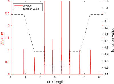
(a) $f_{3}$ with $C^{0}$ and $C^{1}$ discontinuities.

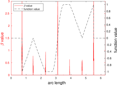
(b) $f_{4}$ with $C^{0}$, $C^{1}$, and $C^{2}$ discontinuities.

Figure 2: Node-based $\beta$ indicator values at discontinuities of example functions.

To address the potential false positiveness, we introduced $\tau$ in (16) as a second threshold. The local threshold $\tau_{\ell}$ in (16) is based on the Taylor series analysis in Section 4.1.1: In smooth regions, $\delta f_{\ell}=\mathcal{O}(h_{\ell})$, so $\delta f_{\ell}h_{\ell}^{0.5}=\mathcal{O}(h_{\ell}^{1.5})$. This term separates the $\alpha$ values at smooth regions, which are $\mathcal{O}(h_{\ell}^{2})$, from those at $C^{0}$ and $C^{1}$ discontinuities, which are $\mathcal{O}(1)$ and $\mathcal{O}(h_{\ell})$, respectively. The use of $h_{\ell}$ (instead of $h_{g}$) makes $\tau_{\ell}$ to be independent of the scaling of the geometry and be insensitive to the nonuniformity of the mesh. Similarly, the use of the local range $\delta f_{\ell}$ makes $\tau_{l}$ independent of scaling of $f$. However, if the function is locally nearly a constant, then $\delta f_{\ell}\approx 0$, so $\tau_{\ell}$ would fail to filter out the false positiveness in such cases. In (16), $\tau_{g}$ is a safeguard for such cases, where $\delta f_{g}h_{g}^{1.5}=\mathcal{O}(h_{g}^{1.5})$ on quasiuniform meshes. In terms of the constant values $C_{\ell}$ and $C_{g}$, too large values can result in false negativeness, and too small values can lead to some false positiveness. For robustness, we chose $C_{\ell}=0.5$ and $C_{g}=0.05$, which are large enough to avoid virtually all false positiveness on sufficiently fine meshes without introducing false negativeness.

4.1.4 Node-based markers on target mesh

After obtaining the node-based markers, it is then straightforward to map them to nodal markers on the target mesh. In particular, given a target node $v$, if any of the source node in its stencil is marked as discontinuities, we mark $v$ as a discontinuity on the target mesh. This step further improves the robustness of the detection step, in that some isolated false negativeness on the source mesh can be corrected if any of their neighbor nodes is marked correctly.

With a robust marker of discontinuities, one can apply various limiters near discontinuities. For example, to preserve monotonicity near discontinuities, we can bound the solution at a target node near discontinuities to be bounded by the local extreme values of its containing element on the source mesh. However, using such a limiter alone is insufficient by itself. It is desirable to adapt the weighting scheme near the detected discontinuities.

4.2 New weighting scheme for WLS-ENO

After detecting the discontinuous regions, we resolve the potential Gibbs phenomena from WLS with scaled Buhmann weights. Our basic idea is motivated by WLS-ENO in [71], which adapts the weights to deprioritize the nodes that are on the other side of discontinuities. We propose a modification to the weighting scheme to take into account the element-based $\alpha$ values. In particular, for the $j$th node in the stencil of node $v$ on the target mesh, we define the weight to be

$$\omega_{j}^{\text{ENO}}=\frac{\gamma_{j}^{+}\left(r_{j}^{2}+\epsilon_{\text{ID}}\right)^{-1/4}}{c_{0}\left|f_{j}-g_{0}\right|^{2}+c_{1}\delta f_{g}\max_{v_{j}\in e}\left|\alpha_{e}\right|+\epsilon_{\text{ENO}}\delta f_{g}^{2}\bar{h}^{2}},$$ (17)

where $f_{j}$ denotes the function value at the node in the source mesh, $g_{0}$ denotes the linear interpolation at node $v$ from the source mesh, and $\epsilon_{\text{ENO}}\bar{h}^{2}$ serves a safeguard against division by a too small value. The scaling by the different powers of $\delta f_{g}$ in the denominator consistent units of all the terms for smooth functions, so that the weighting scheme is invariant of shifting and scaling of the input function. We use $\epsilon_{\text{ENO}}=10^{-3}$ and let $\bar{h}$ be the average distance length in the local $uv$ coordinate system. In the enumerator, $\gamma_{j}^{+}$, $r_{j}$, and $\epsilon^{\text{ID}}$ are the same as those in the inverse-distance based weight (9).

The definition of $\omega_{j}^{\text{ENO}}$ was guided by an asymptotic analysis, which we outline as follows. Without loss of generality, let us first assume the enumerator is $1$. If $c_{0}=1$ and $c_{1}=0$, then $\omega_{j}^{\text{ENO}}$ is essentially the same as that in [71] for hyperbolic conservation laws, except that we use linear interpolation to obtain $g_{0}$ in remap. With those parameters, $\omega_{j}^{\text{ENO}}=\mathcal{O}(1)$, $\mathcal{O}(h^{-2})$ and $\mathcal{O}(h^{-2})$ at $C^{0}$ discontinuities, $C^{1}$ discontinuities, and smooth regions, respectively, so it could not distinguish $C^{1}$ discontinuities from smooth regions. When $c_{1}\neq 0$, however, since $\max_{v_{j}\in e}\left|\alpha_{e}\right|=\mathcal{O}(h)$ at $C^{1}$ discontinuities, $\omega_{j}^{\text{ENO}}=\mathcal{O}(1)$, $\mathcal{O}(h^{-1})$ and $\mathcal{O}(h^{-2})$ at $C^{0}$ discontinuities, $C^{1}$ discontinuities, and smooth regions, respectively. Note that the denominator of (17) does not take into account distance or normals. As in (9), $\gamma_{j}^{+}$ serves as a safeguard for sharp features or under-resolved high-curvature regions in surface meshes. The inverse-distance part of the enumerate introduces an $\mathcal{O}(\sqrt{h})$ term, which would still allow $\omega_{j}^{\text{ENO}}$ to distinguish discontinuities from smooth regions while reducing the influence of far-away points and in turn reduce the potential interference of nearby discontinuities.

To obtain the parameters in $\omega_{j}^{\text{ENO}}$, we conducted numerical experimentation and found that $c_{0}=1$ and $c_{1}=0.05$ worked well in practice. For robustness and efficiency, we use quadratic WLS-ENO near discontinuities with $3$-rings, same as the ring size for quartic WLS-ENO in smooth regions. With these parameters, our proposed WLS-ENO scheme is relatively insensitive to false positiveness of detected discontinuities. This is because even if all the nodes are marked as discontinuities, the WLS-ENO weights (17) with quadratic WLS would be used, and the method is still third-order accurate for smooth functions, which is still higher than commonly used low-order methods.

5 Numerical experimentation

In this section, we report numerical experimentation with WLS-ENOR. Since one of our main targeted application areas is climate and earth modeling, we focus on on node-to-node transfer between Delaunay triangulations and cubed-sphere meshes of the unit sphere. The former type is the dual of the spherical centroidal Voronoi tessellations (SCVT) [57], which are commonly used with finite volume methods in ocean modeling. In this setting, the nodal values in the Delaunay mesh are equivalent to cell-centered values in the Voronoi tessellation. The latter type is often used in finite volume [79] or spectral element methods [97] in atmospheric models. We assess WLS-ENOR for both smooth and discontinuous functions under different mesh resolutions. To this end, we generated a series these meshes of different resolutions using Ju’s SCVT code [57] and equidistant gnomonic projection of sphere [86], respectively. Figure 3 shows the coarsest meshes used in our tests, which we refer to as the level-1 meshes. The Delaunay mesh has 4,096 nodes and 8,188 triangles, and the cubed-sphere mesh has 1,016 nodes and 1,014 quadrilaterals, respectively. For each level of mesh refinement, the number of triangles or quadrilaterals quadruples.

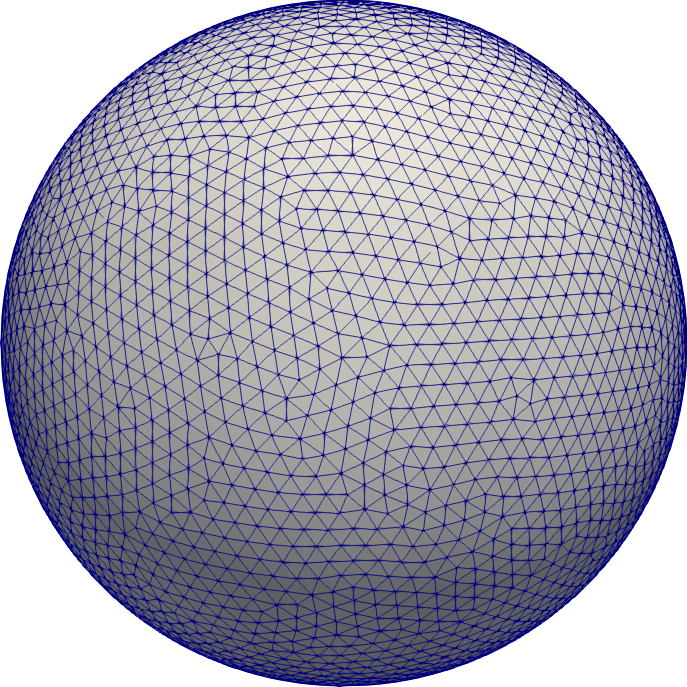
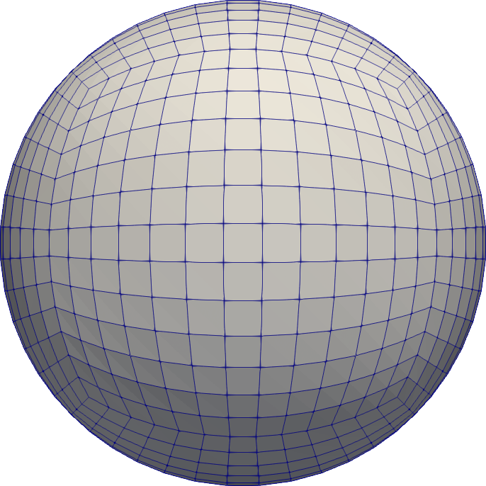
Figure 3: Coarsest Delaunay and cubed-sphere meshes used in our tests.

5.1 Transferring smooth functions

We first consider WLS-based transfer for smooth functions. We report some representative results with two functions, namely,

$$f_{1}(x,y,z)=\left(\sin(\pi x)+\cos(\pi y)\right)z$$ (18)

and

$$f_{2}(x,y,z)=\left(11z^{2}-1\right)\left(x^{4}-6x^{2}y^{2}+y^{2}\right).$$ (19)

The latter is the real part of an unnormalized version of the degree-$6$ spherical harmonic function $Y_{6}^{4}(\theta,\varphi)$ [104], i.e.,

$$f_{2}\left(\theta,\varphi\right)=\text{Re}\left(e^{4i\varphi}\sin^{4}\theta\left(11\cos^{2}\theta-1\right)\right),$$ (20)

where $\theta\in[0,\pi$] and $\varphi\in[0,2\pi]$ are the polar (colatitudinal) and the azimuthal (longitudinal) angles, respectively. For smooth functions, we consider the $\ell^{2}$-norm error. Let $\boldsymbol{e}$ denote the vector composed of the pointwise error for each node of a mesh, and let $N$ denote the number of nodes. The $\ell^{2}$-norm error is measured as

$$\left\|\boldsymbol{e}\right\|_{\ell_{2}}=\frac{1}{\sqrt{N}}\left\|\boldsymbol{e}\right\|_{2}=\sqrt{\frac{1}{N}\sum_{i=1}^{N}e_{i}^{2}}.$$ (21)

Given two meshes of different resolutions with $N_{1}$ and $N_{2}$ nodes, where $N_{1}<N_{2}$, and let $\boldsymbol{e}_{1}$ and $\boldsymbol{e}_{2}$ denote their respective error vectors. Assuming the meshes are uniformly, which is the case in our tests, we evaluate the convergence rate in $\ell_{2}$ norm between the two meshes as

$$\text{convergence rate}=2\frac{\log(\left\|\boldsymbol{e}_{1}\right\|_{\ell_{2}}/\left\|\boldsymbol{e}_{2}\right\|_{\ell_{2}})}{\log(N_{2}/N_{1})},$$ (22)

which is equivalent to the standard definition based on edge length. Although we recommend quartic WLS in smooth regions, we will report results with quadratic, quartic, and sextic WLS for completeness and for comparison.

5.1.1 Numerical optimization of cut-off radii

One of the key aspect of our WLS transfer is its weighting scheme, namely the scaled Buhmann weights described in Section 3.3. Here, we describe our procedure to optimize the cut-off radius $\rho=\sigma R$ in these weights. Our goal is to minimize the $\ell^{2}$-norm error of the transferred solution with respect to $\sigma$. It is difficult, if not impossible, to write down an equation for this objective function, because $R$ depends on the combinatorial structure of the mesh. Fortunately, a precise $\sigma$ is unnecessary, so we solve this optimization problem approximately by using the two example $f_{1}$ and $f_{2}$ in (18) and (19) and the Delaunay and cubed-sphere meshes depicted in Figure 3. We transferred the functions between the meshes for $\sigma$ between 1 and 3 with an increment of $0.1$. Figure 4 shows the $\ell^{2}$ norm errors of degree-2, 4, and 6 WLS in transferring from the Delaunay to the cubed-sphere mesh. It is evident that the error profile had a “V” shape with respect to $\sigma$ for both functions, and the minima were at $\sigma=2.0$, $1.6$ and $1.4$ for degree-2, 4, and 6 WLS, respectively. As a reference, Figure 4 also shows the errors with the inverse-distance based weights (9). The scaled Buhmann weights with optimal $\sigma$ improved the accuracy by nearly two orders of magnitude compared to using (9). It is also worth noting that the optimal $\sigma$ values remained about the same when we transferred other smooth functions, transferred from the cubed-sphere to the Delaunay meshes, or used different mesh resolution. This shows that the numerical optimization is well posed for smooth functions with a sufficiently smooth weight function.

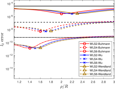
(a) Error profiles for $f_{1}$ in (18).

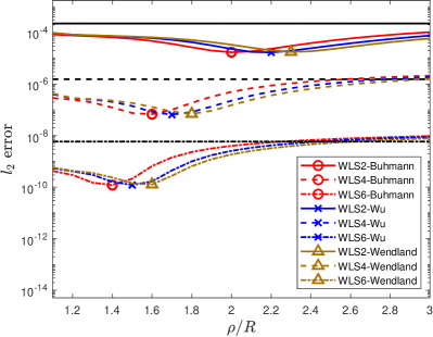
(b) Error profiles for $f_{2}$ in (19).

Figure 4: $\ell^{2}$-norm errors in degree-2, 4, and 6 WLS with respect to the radius ratio $(\sigma=\rho/R)$ in weights based on Buhmann’s $C^{3}$, Wu’s $C^{4}$, and Wendland’s $C^{4}$ radial functions. The marks indicate the optimal $\sigma$ values for each weighting strategy.

We also applied the optimization procedure to other radial functions, including those in [106] and [102]. We observed that the well-posedness of our optimization procedure required at least $C^{3}$ continuity. For comparison, Figure 4 also shows the error profiles with the following two weighting schemes:

$$w_{j}=\gamma_{j}^{+}\phi_{2,0}(r_{j}/\rho),\,\text{where}\,\phi_{2,0}(r)=\left(1-r\right)_{+}^{5}\left(r^{4}+5r^{3}+9r^{2}+5r+1\right),$$ (23)

and

$$w_{j}=\gamma_{j}^{+}\psi_{4,2}(r_{j}/\rho),\text{ where }\psi_{4,2}(r)=\left(1-r\right)_{+}^{6}\left(35r^{2}+18r+3\right).$$ (24)

The radial functions $\phi_{2,0}$ and $\psi_{4,2}$ are $C^{4}$ functions due to Wu [106] and Wendland [102], respectively. It is clear that the scaled Buhmann weights had the smallest optimal cut-off radii, which result in smaller constant factors in the leading error term and also fewer rows in the generalized Vandermonde systems. The $C^{6}$ functions of Wu and Wendland required even larger cut-off radii. Hence, the scaled Buhmann weights are the overall winners in both accuracy and efficiency for WLS-based remapping. We note that DTK contains a collection of weights, which were mostly based on Wu’s and Wendland’s functions, and DTK requires the user to choose the specific weights and the cut-off radius [94]. In contrast, our approach is parameter-free from the user’s perspective, in that both the weighting functions and cut-off radii were pre-optimized.

5.1.2 Accuracy and convergence

We first assess the accuracy and convergence of WLS for smooth functions in comparison with several other data-transfer methods, including linear interpolation, common-refinement-based $L^{2}$ projection [49], MMLS in DTK [94], and RBF interpolation [4]. For MMLS, we used the same parameters as recommended in [94], with Wu’s $C^{4}$ radial function as weights and a cut-off radius of about five times the maximum edge length on the source mesh. For RBF interpolation, we used the implementation in DTK as described in [94]. However, we adhered to the original formulation of Beckert and Wendland in [4] with Wendland’s $C^{2}$ radial functions (instead of using Wu’s $C^{4}$ functions as in [94]). We set the cut-off radius for RBF to be five times the maximum edge length on both source and target meshes, which was significantly larger than the recommendation in [4] but was necessary for the solution to be stable and reasonably accurate. For convergence study, we used four sets of triangular and quadrilateral meshes with different resolutions. Figure 5 shows the $\ell^{2}$-norm errors of each of these methods together with quadratic, quartic, and sextic WLS for functions $f_{1}$ and $f_{2}$. For completeness, we also show the result with cubic WLS, for which we used its optimal radius ratio $\sigma=1.2$. The number associated with each line segment indicates the convergence rate for its corresponding method under the corresponding mesh refinement.

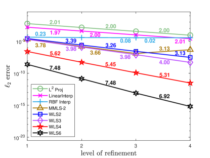
(a) Errors for $f_{1}$ in (18).

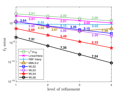
(b) Errors for $f_{2}$ in (19).

Figure 5: Comparison of accuracy and convergence of remap methods under mesh refinement.

We make several observations from the results. First, both $L^{2}$ projection and linear interpolation achieved second-order accuracy. Note that on surface meshes, $L^{2}$ projection involves geometric errors in its integration, so its accuracy was slightly worse that that of linear interpolation, unlike the 2-D results in [49]. The RBF interpolation of Beckert and Wendland produced smaller errors than linear interpolation and $L^{2}$ projection, but its overall convergence rate was close to zero. Note that MMLS in DTK uses quadratic polynomials in the global $xyz$ coordinate system, which have the same number of coefficients as cubic WLS in the local $uv$ coordinate. As a result, MMLS performed slightly better than quadratic WLS on the three coarser meshes but worse than cubic WLS. More importantly, DTK lost convergence on the finest mesh, because the nearly planar stencils on fine meshes lead to nearly singular Vandermonde systems. Although DTK uses truncated SVD (TSVD) to resolve ill-conditioning algebraically, the convergence was lost due to the random truncation of low-degree terms by TSVD. In contrast, we use local 2D coordinate systems within the local tangent space and use QRCP to solve the linear system, and we truncate the highest-degree terms in the presence of ill-conditioning. Hence, WLS is both stable and accurate, even when using degree-6 polynomials, of which the solution achieved machine precision on the finest mesh.

5.1.3 Accuracy and conservation in repeated transfer

The preceding section focused on accuracy and convergence in a single-step transfer. In multiphysics applications, data must be exchanged between meshes repeated. Hence, it is important to take into account the accuracy and convergence in such a setting. Figure 6 compared the accuracy when transferring smooth functions back and forth for 1000 times between the Delaunay and cubed-sphere meshes. Because MMLS was unstable and RBF was computationally too expensive on the finest mesh, we only report results on the three coarser meshes. Quartic and sextic WLS clearly stand out in their accuracy. Among the other methods, linear interpolation became far less accurate in repeated transfer. RBF interpolation performed better than linear interpolation, but its convergence rate was close to zero. $L^{2}$ projection was remarkably accurate compared to all the other third or lower-order methods, especially on coarse meshes, due to its conservation property. Note that MMLS exhibited better accuracy than quadratic WLS but similar accuracy as cubic WLS in repeated transfer. This is because MMLS with quadratic polynomials in the global $xyz$ coordinate systems has the same number of monomial basis functions as WLS with cubic polynomials in the local $uv$ coordinate system.

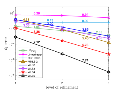
(a) Errors for $f_{1}$ in (18).

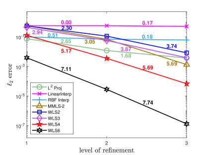
(b) Errors for $f_{2}$ in (19).

Figure 6: Accuracy and convergence on Delaunay mesh after 1000 steps of repeated transfers.

Besides accuracy, another important consideration for repeated transfer is conservation [18, 49]. Unfortunately, the conservation error is not uniquely defined, especially for high-order methods. In this work, we measure the conservation error as the difference between the integral of the exact function and that of final reconstructed function. We use numerical quadrature to compute the integrals the exact spherical geometry, where we evaluated the values at the quadrature points using the same-degree of WLS for quartic and sextic WLS and using quadratic WLS reconstruction for all the other methods. Figure 7 compares the conservation errors on the level-2 and level-3 meshes for $f_{2}$. Linear interpolation performed the worst due to its low-order accuracy and non-conservation. $L^{2}$ projection was not strictly conservative primarily because its numerical integration is inexact on spheres, but it was nevertheless more conservative than MMLS and WLS-2, although less conservative than WLS-3. RBF interpolation was competitive with $L^{2}$ projection in terms of conservation, despite its lower accuracy. Quartic and sextic WLS were more conservative than $L^{2}$ projection on surfaces, although they do not enforce conservation explicitly.

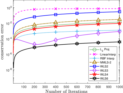
(a) Level-2 mesh.

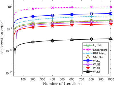
(b) Level-3 mesh.

Figure 7: Evolution of conservation errors in repeated transfer for $f_{2}$.

5.2 Transferring discontinuous functions

To assess the treatment of discontinuities, we use two piecewise smooth functions, namely

$$f_{3}\left(\theta,\varphi\right)=\begin{cases}\begin{array}[]{c}1\\ 1-0.8\left(\theta-0.87\right)\\ 0.44\\ 0.24\\ 0.12\end{array}&\begin{array}[]{c}0\leq\theta<0.87\\ 0.87\leq\theta<\pi/2\\ \pi/2\leq\theta<2.27\\ 2.27\leq\theta<2.83\\ 2.83\leq\theta\leq\pi\end{array}\end{cases},$$ (25)

and

$$f_{4}\left(\theta,\varphi\right)=-1000+g(\varphi)\begin{cases}0&0\leq\theta<\pi/4\\ -4\left(\theta/\pi-1/2\right)&\pi/4\leq\theta<\pi/2\\ 4\left(\theta/\pi-1/2\right)&\pi/2\leq\theta<3\pi/4\\ 1&3\pi/4\leq\theta<7\pi/8\\ -64\theta^{2}/\pi^{2}+112\theta/\pi-48&7\pi/8\leq\theta\leq\pi\end{cases},$$ (26)

with $g\left(\varphi\right)=\begin{cases}-2000&0\leq\varphi<\pi\\ 2000&\pi\leq\varphi\leq 2\pi\end{cases}$. Function $f_{3}$ is an axial-symmetric function with both $C^{0}$ and $C^{1}$ discontinuities in the $\theta$ direction, which are similar to an intermediate solution of two interacting blast waves [47]. Hence, we refer to $f_{3}$ as interacting waves. Function $f_{4}$ has a richer structure of discontinuities, including $C^{0}$, $C^{1}$, and $C^{2}$ discontinuities in the $\theta$ direction, which intersect with the $C^{0}$ discontinuities in the $\varphi$ direction. Hence, we refer to $f_{4}$ as crossing waves. The range of $f_{3}$ is between $0.12$ and 1, and that of $f_{4}$ is approximately between $-3000$ and $1000$. The disparate ranges allow us to demonstrate the independence of scaling and shifting of the function values of our method. Figure 8 shows these functions on the level-4 Delaunay mesh. Figure 9 shows the detected discontinuities on the level-4 cubed-sphere mesh, computed from the indicators on the Delaunay mesh. All the $C^{0}$ and $C^{1}$ discontinuities were detected correctly on this mesh. We note that they were also detected correctly on the coarser meshes. These results demonstrate the low (nearly zero) false-negative rate of our detection technique. In addition, our technique also has a low false-positive rate, which is evident in Figure 9, where the $C^{2}$ discontinuities in $f_{4}$ were not marked. We also tested our discontinuity indicators for the smooth functions $f_{1}$ and $f_{2}$ on all the meshes, and no false discontinuity was marked on any of the meshes. Hence, our detection technique is robust in terms of both false-negative and false-positive rates.

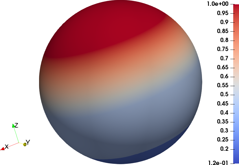
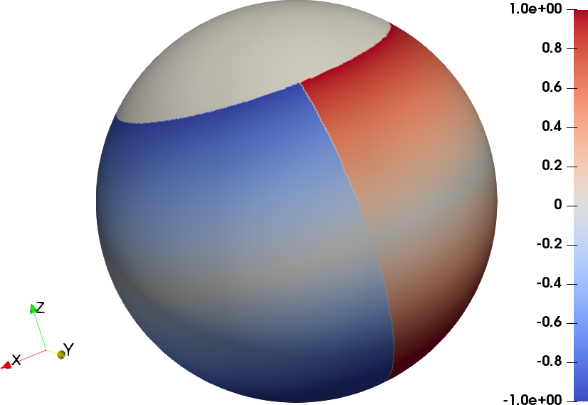
Figure 8: Discontinuous functions $f_{3}$ (left) and $f_{4}$ on level-4 Delaunay mesh.

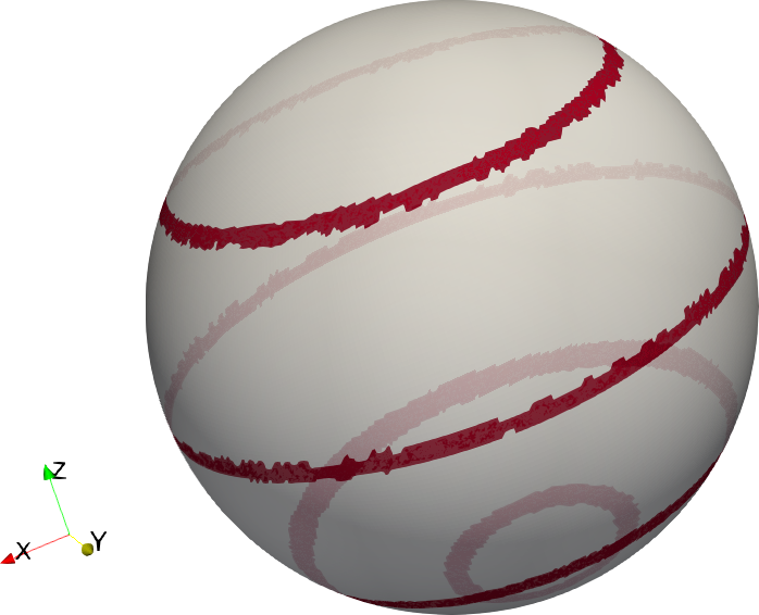
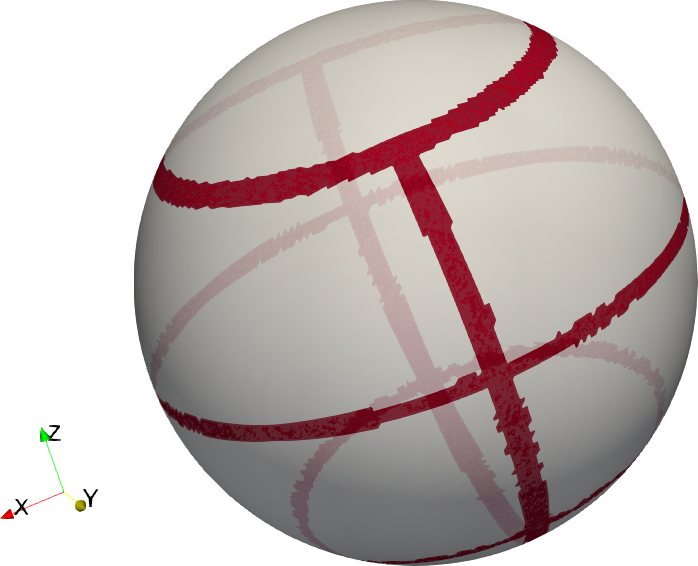
Figure 9: Detected discontinuities for $f_{3}$ (left) and $f_{4}$ on level-4 cubed-sphere mesh.

5.2.1 Justification of WLS-ENO degree and weights

In WLS-ENOR, we use quartic WLS in smooth regions and quadratic WLS-ENO near discontinuities. We refer to this combination as WLS-ENOR(4,2). As we have shown in Section 5.1, quartic WLS delivers high accuracy and conservation for smooth functions. We now justify the use of quadratic polynomials by comparing it with WLS-ENOR(4,1) and WLS-ENOR(4,3), i.e., using quartic WLS in smooth regions but linear or cubic WLS-ENO near discontinuities. For WLS-ENOR($p$,$q$), we used $\lfloor 1.5p\rfloor/2$-rings for smooth regions and $(q+0.5)$-rings for discontinuities. We transferred $f_{3}$ back and forth between the level-3 Delaunay and cubed-sphere meshes. Figure 10 shows the results after 500 and 1000 iterations along a great circle passing through the poles, where the dotted solid line shows the “exact” solution. It is clear that WLS-ENOR(4,1) is overly diffusive at the global minimum, although it worked well at other discontinuities. On the other hand, WLS-ENOR(4,3) is less diffusive than WLS-ENOR(4,2) near $C^{1}$ discontinuities, but it had a significant undershoot at the global minimum where two $C^{0}$ discontinuities interact. Note that this undershoot would vanish on the level-4 meshes, indicating that WLS-ENOR(4,3) requires finer meshes than WLS-ENOR(4,2) to separate $C^{0}$ discontinuities. Overall, WLS-ENOR(4,2) delivered a good balance between robustness for coarser meshes and accuracy on finer meshes, so we use it as the default.

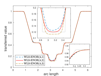
(a) After 500 steps on level-3 mesh.

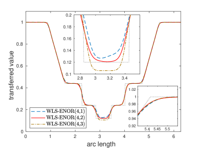
(b) After 1000 steps on level-3 mesh.

Figure 10: Comparison of WLS-ENOR(4,$q$) for $q=1$, $2$, and $3$ in repeated transfer of $f_{3}$ between level-3 Delaunay and cubed-sphere meshes.

In WLS-ENOR, we introduced a new weighting scheme (17), which takes into account $C^{1}$ discontinuities and controls it using the parameter $c_{1}$. To demonstrate its importance, Figure 11 compares WLS-ENOR with and without $c_{1}$ enabled after 500 and 1000 steps in repeated transfer of $f_{4}$ on the level-4 mesh. It can be seen that when not considering the $C^{1}$ discontinuities (i.e., $c_{1}=0$), the solution was less controlled near $C^{1}$ discontinuities. With our default nonzero $c_{1}$, the remap is more robust, and the solution approximates the exact solution very well even after 1000 steps of repeated transfer.

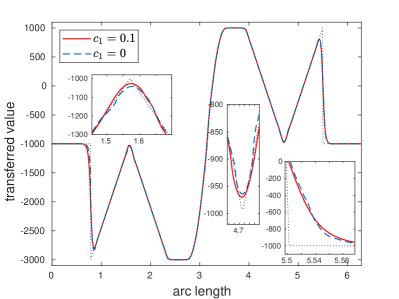
(a) After 500 steps on level-4 mesh.

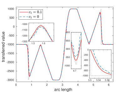
(b) After 1000 steps on level-4 mesh.

Figure 11: Comparison of WLS-ENOR with and without explicit $C^{1}$ treatment in weighting scheme in repeated transfer of $f_{4}$ between level-4 Delaunay and cubed-sphere meshes.

5.2.2 Gibbs phenomena in one-step transfer

We now compare WLS-ENOR with some other methods in transferring discontinuous function. In particular, we compare WLS-ENO(4,2) with the same methods used in Section 5.1 by transferring $f_{3}$ from the level-3 Delaunay to the level-3 cubed-sphere mesh. Figure 12 shows the result on the cubed-sphere mesh along a great circle passing through the poles. We plot WLS-ENO together with linear interpolation in Figure 12(a), because both are non-oscillatory. As can be seen in Figure 12(b–d), MMLS had visible overshoots and undershoots, although they were less severe than those of $L^{2}$ projection and RBF interpolation.

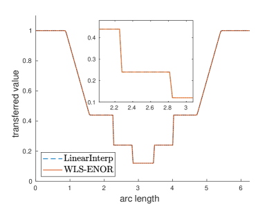
(a) WLS-ENOR and linear interpolation.

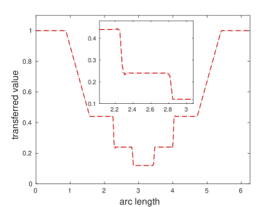
(b) Modified moving least squares (DTK) [94].

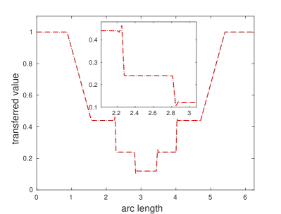
(c) $L^{2}$ projection [49].

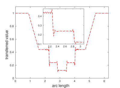
(d) RBF interpolation [4].

Figure 12: Comparison of transferring $f_{3}$ from level-3 Delaunay to cubed-sphere mesh.

5.2.3 Gibbs phenomena and diffusion in repeated transfer

We now compare repeated transfer of discontinuous functions with the least oscillatory methods in the preceding section, namely, WLS-ENOR, linear interpolation, and MMLS; we refer readers to [94] for some comparison of MMLS, $L^{2}$ projection, and RBF interpolation for repeated transfer of discontinuous functions. Figure 13 shows the results on the level-3 meshes after 500 and 1000 steps of repeated transfer between the level-3 Delaunay and cubed-sphere meshes for function $f_{3}$. WLS-ENOR performed the best in terms of both preserving monotonicity and minimizing diffusion. In contrast, linear interpolation was excessively diffusive, whereas MMLS was oscillatory and had a severe undershoot at the global minimum and a noticeable overshoot at the global maximum.

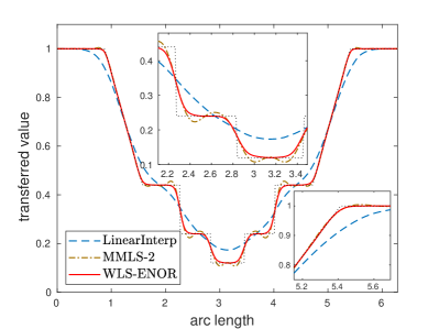
(a) After 500 steps on level-3 mesh.

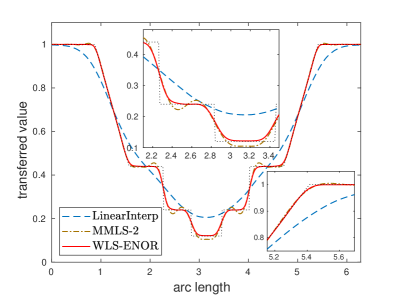
(b) After 1000 steps on level-3 mesh.

Figure 13: Comparison of diffusion of WLS-ENOR versus linear interpolation and MMLS in repeated transfer of $f_{3}$ between level-3 Delaunay and cubed-sphere meshes.

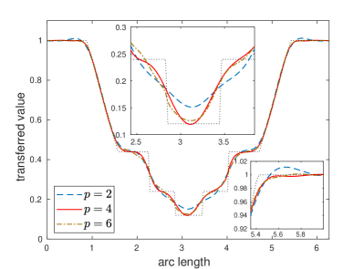
(a) After 1000 iterations on level-2 mesh.

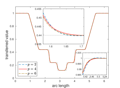
(b) After 1000 iterations on level-4 mesh.

Figure 14: Comparison of WLS-ENOR($p$,2) with $p=2$, 4, and 6 after 1000 repeated transfers for $f_{3}$ between Delaunay and cubed-sphere meshes.

Finally, we report a comparison of WLS-ENOR using different degree of polynomials in smooth regions. Figure 14 shows the results with quadratic, quartic, and sextic WLS (i.e., WLS-ENOR($p$,2) with $p=2$, 4, and 6) after 1000 steps of repeated transfer of function $f_{4}$ on the level-2 and level-4 meshes. On the level-2 mesh, quadratic WLS was significantly more diffusive than the others near the global minimum, where two $C^{0}$ discontinuities interact. It also had some overshoots near $C^{1}$ discontinuities. This is because quadratic WLS does not have sufficient accuracy on coarser meshes. Quartic and sextic WLS produced similar results in smooth regions and near $C^{1}$ discontinuities. However, sextic WLS is more expensive, and it was more diffusive than quartic WLS on the level-2 mesh, This is because sextic WLS requires about 20 cells between $C^{0}$ discontinuities to avoid interference from each other, but quartic WLS requires about 16 cells. These results show that WLS-ENOR(4,2) strikes a good balance between accuracy, efficiency, and robustness.

6 Conclusions

In this paper, we proposed a new method, called WLS-ENO Remap or WLS-ENOR in short, for transferring data between non-matching meshes. The method utilizes quartic WLS reconstruction in smooth regions, and it selectively applies quadratic WLS-ENO reconstruction near discontinuities. For smooth functions, we proposed a new weighting scheme based on Buhmann’s $C^{3}$ radial function and optimized it to enable superconvergence of WLS remap for smooth functions. For discontinuous functions, we proposed a robust technique to detect $C^{0}$ and $C^{1}$ discontinuities with two novel indicators and a new dual-thresholding strategy. We also proposed a new weighting scheme for WLS-ENO to take into account $C^{1}$ discontinuities for robustness. Overall, WLS-ENOR achieves higher than fifth-order accuracy and highly conservative in smooth regions, and is non-oscillatory and minimally diffusive near discontinuities. It compares favorably with other commonly used node-to-node remap techniques in accuracy, stability, conservation, and monotonicity-preservation for almost all of our test cases.

In this work, we primarily focused on node-to-node transfer on spheres, which is most relevant to climate and earth-system modeling. We plan to extend the work to address cell-averaged data, which are commonly used in finite volume methods. Future work will also include extending our method to support more general surfaces, including those with geometric discontinuities, such as ridges and corners, as well as those with boundaries.

References

- [1] A. Adam, D. Pavlidis, J. R. Percival, P. Salinas, Z. Xie, F. Fang, C. C. Pain, A. Muggeridge, and M. D. Jackson. Higher-order conservative interpolation between control-volume meshes: Application to advection and multiphase flow problems with dynamic mesh adaptivity. J. Comput. Phys., 321:512–531, 2016.
- [2] R. Archibald, A. Gelb, and J. Yoon. Polynomial fitting for edge detection in irregularly sampled signals and images. SIAM J. Numer. Ana., 43(1):259–279, 2005.
- [3] R. Archibald, A. Gelb, and J. Yoon. Determining the locations and discontinuities in the derivatives of functions. Appl. Numer. Math., 58(5):577–592, 2008.
- [4] A. Beckert and H. Wendland. Multivariate interpolation for fluid-structure-interaction problems using radial basis functions. Aerosp. Sci. Technol., 5(2):125–134, 2001.
- [5] P. Bochev and M. Shashkov. Constrained interpolation (remap) of divergence-free fields. Comput. Meth. Appl. Mech. Engrg., 194(2-5):511–530, 2005.
- [6] M. Bozzini, L. Lenarduzzi, M. Rossini, and R. Schaback. Interpolation with variably scaled kernels. IMA J. Numer. Ana., 35(1):199–219, 2014.
- [7] M. Bozzini and M. Rossini. The detection and recovery of discontinuity curves from scattered data. J. Comput. Appl. Math., 240:148–162, 2013.
- [8] M. Buhmann. A new class of radial basis functions with compact support. Math. Comput., 70(233):307–318, 2001.
- [9] M. D. Buhmann. Radial basis functions. Acta Numer., 9:1–38, 2000.
- [10] M. D. Buhmann. Radial Basis Functions: Theory and Implementations, volume 12. Cambridge University Press, 2003.
- [11] H.-J. Bungartz, F. Lindner, B. Gatzhammer, M. Mehl, K. Scheufele, A. Shukaev, and B. Uekermann. preCICE – a fully parallel library for multi-physics surface coupling. Comput. Fluids, 141:250–258, 2016.
- [12] J. Canny. A computational approach to edge detection. In Readings in Computer Vision, pages 184–203. Elsevier, 1987.
- [13] D. Cates and A. Gelb. Detecting derivative discontinuity locations in piecewise continuous functions from fourier spectral data. Numer. Algo., 46(1):59–84, 2007.
- [14] G. Chesshire and W. D. Henshaw. A scheme for conservative interpolation on overlapping grids. SIAM J. Sci. Comput., 15(4):819–845, 1994.
- [15] B. Cockburn, G. E. Karniadakis, and C.-W. Shu. The Development of Discontinuous Galerkin Methods. Springer, 2000.
- [16] P. Colella and P. R. Woodward. The piecewise parabolic method (PPM) for gas-dynamical simulations. J. Comput. Phys., 54(1):174–201, 1984.
- [17] A. Craig, S. Valcke, and L. Coquart. Development and performance of a new version of the OASIS coupler, OASIS3-MCT_3. 0. Geosci. Model Dev., 10(9):3297–3308, 2017.
- [18] A. de Boer, A. H. van Zuijlen, and H. Bijl. Comparison of conservative and consistent approaches for the coupling of non-matching meshes. Comput. Methods Appl. Mech. Eng., 197(49-50):4284–4297, 2008.
- [19] C. de Boor. Quasiinterpolants and approximation power of multivariate splines. In Computation of curves and surfaces, pages 313–345. Springer, 1990.
- [20] M. C. L. de Silanes, M. C. Parra, and J. J. Torrens. Vertical and oblique fault detection in explicit surfaces. J. Comput. Appl. Math., 140(1-2):559–585, 2002.
- [21] V. Dyedov, N. Ray, D. Einstein, X. Jiao, and T. Tautges. AHF: Array-based half-facet data structure for mixed-dimensional and non-manifold meshes. In J. Sarrate and M. Staten, editors, Proceedings of the 22nd International Meshing Roundtable, pages 445–464. Springer International Publishing, 2014.
- [22] P. Farrell and J. Maddison. Conservative interpolation between volume meshes by local Galerkin projection. Comput. Meth. Appl. Mech. Engrg., 200(1-4):89–100, 2011.
- [23] P. Farrell, M. Piggott, C. Pain, G. Gorman, and C. Wilson. Conservative interpolation between unstructured meshes via supermesh construction. Comput. Meth. Appl. Mech. Engrg., 198(33-36):2632–2642, 2009.
- [24] S. Fleishman, D. Cohen-Or, and C. T. Silva. Robust moving least-squares fitting with sharp features. ACM Trans. Graph., 24(3):544–552, 2005.
- [25] N. Flyer and G. B. Wright. Transport schemes on a sphere using radial basis functions. J. Comput. Phys., 226(1):1059–1084, 2007.
- [26] B. Fornberg and N. Flyer. The Gibbs phenomenon for radial basis functions. The Gibbs Phenomenon in Various Representations and Applications, pages 201–224, 2007.
- [27] J. Foster and F. Richards. The Gibbs phenomenon for piecewise-linear approximation. Amer. Math. Monthly, 98(1):47–49, 1991.
- [28] M. J. Gander and C. Japhet. Algorithm 932: PANG: software for nonmatching grid projections in 2D and 3D with linear complexity. ACM Trans. Math. Softw., 40(1):6, 2013.
- [29] A. Gelb and E. Tadmor. Detection of edges in spectral data. Appl. Comput. Harmon. Anal., 7(1):101–135, 1999.
- [30] A. Gelb and E. Tadmor. Detection of edges in spectral data ii. nonlinear enhancement. SIAM J. Numer. Anal., 38(4):1389–1408, 2000.
- [31] A. Gelb and E. Tadmor. Adaptive edge detectors for piecewise smooth data based on the minmod limiter. J. Sci. Comput., 28(2-3):279–306, 2006.
- [32] J. W. Gibbs. Letter to the editor. Nature, page 200 and 606, 1899.
- [33] S. K. Godunov. A difference method for numerical calculation of discontinuous solutions of the equations of hydrodynamics. Mat. Sb., 89(3):271–306, 1959.
- [34] G. H. Golub and C. F. Van Loan. Matrix Computations. Johns Hopkins, 4th edition, 2013.
- [35] D. Gottlieb and C.-W. Shu. On the Gibbs phenomenon and its resolution. SIAM Rev., 39(4):644–668, 1997.
- [36] S. Gottlieb and C.-W. Shu. Total variation diminishing Runge-Kutta schemes. Math. Comput., 67(221):73–85, 1998.
- [37] J. Grandy. Conservative remapping and region overlays by intersecting arbitrary polyhedra. J. Comput. Phys., 148(2):433–466, 1999.
- [38] R. L. Harder and R. N. Desmarais. Interpolation using surface splines. J. Aircraft, 9(2):189–191, 1972.
- [39] A. Harten. ENO schemes with subcell resolution. J. Comput. Phys., 83(1):148–184, 1989.
- [40] E. Hewitt and R. E. Hewitt. The Gibbs-Wilbraham phenomenon: an episode in Fourier analysis. Arch. Hist. Exact Sci., 21(2):129–160, 1979.
- [41] N. J. Higham. A survey of condition number estimation for triangular matrices. SIAM Rev., 29:575–596, 1987.
- [42] C. Hill, C. DeLuca, M. Suarez, A. Da Silva, et al. The architecture of the earth system modeling framework. Comput. Sci. Engrg., 6(1):18, 2004.
- [43] C. Hu and C.-W. Shu. Weighted essentially non-oscillatory schemes on triangular meshes. J. Comput. Phys., 150(1):97–127, 1999.
- [44] J. Humpherys, T. J. Jarvis, and E. J. Evans. Foundations of Applied Mathematics, Volume I: Mathematical Analysis. SIAM, 2017.
- [45] J. W. Hurrell, M. M. Holland, P. R. Gent, S. Ghan, J. E. Kay, P. J. Kushner, J.-F. Lamarque, W. G. Large, D. Lawrence, K. Lindsay, et al. The community earth system model: a framework for collaborative research. B. Am. Meterol. Soc., 94(9):1339–1360, 2013.
- [46] A. J. Jerri. The Gibbs Phenomenon in Fourier Analysis, Splines and Wavelet Approximations, volume 446. Springer, 2013.
- [47] G.-S. Jiang and C.-W. Shu. Efficient implementation of weighted ENO schemes. J. Comput. Phys., 126(1):202–228, 1996.
- [48] X. Jiao, H. Edelsbrunner, and M. T. Heath. Mesh association: formulation and algorithms. In International Meshing Roundtable, pages 75–82. Citeseer, 1999.
- [49] X. Jiao and M. T. Heath. Common-refinement-based data transfer between non-matching meshes in multiphysics simulations. Int. J. Numer. Meth. Engrg., 61(14):2402–2427, 2004.
- [50] X. Jiao and M. T. Heath. Overlaying surface meshes, part I: Algorithms. Int. J. Comput. Geom. Appl., 14(06):379–402, 2004.
- [51] X. Jiao and M. T. Heath. Overlaying surface meshes, part II: Topology preservation and feature matching. Int. J. Comput. Geom. Appl., 14(06):403–419, 2004.
- [52] X. Jiao and D. Wang. Reconstructing high-order surfaces for meshing. Engrg. Comput., 28:361–373, 2012.
- [53] X. Jiao and H. Zha. Consistent computation of first- and second-order differential quantities for surface meshes. In ACM Solid and Physical Modeling Symposium, pages 159–170. ACM, 2008.
- [54] G. R. Joldes, H. A. Chowdhury, A. Wittek, B. Doyle, and K. Miller. Modified moving least squares with polynomial bases for scattered data approximation. Appl. Math. Comput., 266:893–902, 2015.
- [55] P. W. Jones. First- and second-order conservative remapping schemes for grids in spherical coordinates. Mon. Weather Rev., 127(9):2204–2210, 1999.
- [56] W. Joppich and M. Kürschner. MpCCI–a tool for the simulation of coupled applications. Concurr. Comp.-Pract. E., 18(2):183–192, 2006.
- [57] L. Ju, T. Ringler, and M. Gunzburger. Voronoi tessellations and their application to climate and global modeling. In Numerical Techniques for Global Atmospheric Models, pages 313–342. Springer, 2011.
- [58] J.-H. Jung. A note on the Gibbs phenomenon with multiquadric radial basis functions. Appl. Numer. Math., 57(2):213–229, 2007.
- [59] J.-H. Jung, S. Gottlieb, and S. O. Kim. Iterative adaptive RBF methods for detection of edges in two-dimensional functions. Appl. Numer. Math., 61(1):77–91, 2011.
- [60] J.-H. Jung and B. D. Shizgal. Generalization of the inverse polynomial reconstruction method in the resolution of the Gibbs phenomenon. J. Comput. Appl. Math., 172(1):131–151, 2004.
- [61] G. Karniadakis and S. Sherwin. Spectral/hp Element Methods for Computational Fluid Dynamics. Oxford University Press, 2013.
- [62] S. E. Kelly. Gibbs phenomenon for wavelets. Appl. Comput. Harmon. Anal., 3(1):72–81, 1996.
- [63] D. E. Keyes, L. C. McInnes, C. Woodward, W. Gropp, E. Myra, M. Pernice, J. Bell, J. Brown, A. Clo, J. Connors, et al. Multiphysics simulations: challenges and opportunities. Int. J. High Perform. Comput. Appl., 27(1):4–83, 2013.
- [64] P. Lancaster and K. Salkauskas. Surfaces generated by moving least squares methods. Math. Comput., 37(155):141–158, 1981.
- [65] P. Lancaster and K. Salkauskas. Surfaces Generated by Moving Least Squares Methods. Mathematics of Computation, 37(155):141 – 158, 1981.
- [66] J. Larson, R. Jacob, and E. Ong. The model coupling toolkit: a new Fortran90 toolkit for building multiphysics parallel coupled models. Int. J. High Perform. Comput. Appl., 19(3):277–292, 2005.
- [67] P. H. Lauritzen and R. D. Nair. Monotone and conservative cascade remapping between spherical grids (cars): Regular latitude–longitude and cubed-sphere grids. Mon. Weather Rev., 136(4):1416–1432, 2008.
- [68] P. H. Lauritzen, R. D. Nair, A. Herrington, P. Callaghan, S. Goldhaber, J. Dennis, J. Bacmeister, B. Eaton, C. Zarzycki, M. A. Taylor, et al. NCAR release of CAM-SE in CESM2.0: A reformulation of the spectral element dynamical core in dry-mass vertical coordinates with comprehensive treatment of condensates and energy. J. Adv. Model Earth Sy., 10(7):1537–1570, 2018.
- [69] R. J. LeVeque. Numerical Methods for Conservation Laws, volume 132. Springer, 1992.
- [70] Y. Lipman and D. Levin. Approximating piecewise-smooth functions. IMA J. Numer. Ana., 30(4):1159–1183, 2009.
- [71] H. Liu and X. Jiao. WLS-ENO: Weighted-least-squares based essentially non-oscillatory schemes for finite volume methods on unstructured meshes. J. Comput. Phys., 314:749–773, 2016.
- [72] X.-D. Liu, S. Osher, and T. Chan. Weighted essentially non-oscillatory schemes. J. Comput. Phys., 115(1):200–212, 1994.
- [73] Y. Liu and Y.-T. Zhang. A robust reconstruction for unstructured WENO schemes. J. Sci. Comput., 54(2,3):603–621, 2013.
- [74] H. Luo, Y. Xia, S. Spiegel, R. Nourgaliev, and Z. Jiang. A reconstructed discontinuous Galerkin method based on a hierarchical WENO reconstruction for compressible flows on tetrahedral grids. J. Comput. Phys., 236:477–492, 2013.
- [75] V. Mahadevan, I. R. Grindeanu, N. Ray, R. Jain, and D. Wu. SIGMA release v1. 2-capabilities, enhancements and fixes. Technical report, Argonne National Laboratory (ANL), Argonne, IL (United States), 2015.
- [76] L. Margolin and M. Shashkov. Second-order sign-preserving conservative interpolation (remapping) on general grids. J. Comput. Phys., 184(1):266–298, 2003.
- [77] A. A. Michelson. Letter to the editor. Nature, 58:544–545, 1898.
- [78] A. Petersen, A. Gelb, and R. Eubank. Hypothesis testing for Fourier based edge detection methods. J. Sci. Comput., 51(3):608–630, 2012.
- [79] W. M. Putman and S.-J. Lin. Finite-volume transport on various cubed-sphere grids. J. Comput. Phys., 227(1):55–78, 2007.
- [80] J. Qiu and C.-W. Shu. A comparison of troubled-cell indicators for Runge–Kutta discontinuous Galerkin methods using weighted essentially nonoscillatory limiters. SIAM J. Sci. Comput., 27(3):995–1013, 2005.
- [81] N. Ray, D. Wang, X. Jiao, and J. Glimm. High-order numerical integration over discrete surfaces. SIAM J. Numer. Ana., 50:3061–3083, 2012.
- [82] T. Rendall and C. Allen. Unified fluid–structure interpolation and mesh motion using radial basis functions. Int. J. Numer. Meth. Engrg., 74(10):1519–1559, 2008.
- [83] F. Richards. A Gibbs phenomenon for spline functions. J. Approx. Theory, 66(3):334–351, 1991.
- [84] L. Romani, M. Rossini, and D. Schenone. Edge detection methods based on RBF interpolation. J. Comput. Appl. Math., 349:532–547, 2019.
- [85] M. Rossini. Interpolating functions with gradient discontinuities via variably scaled kernels. Dolomites Research Notes on Approximation, 11(2), 2018.
- [86] R. Sadourny. Conservative finite-difference approximations of the primitive equations on quasi-uniform spherical grids. Mon. Weather Rev., 100(2):136–144, 1972.
- [87] R. Saxena, A. Gelb, and H. Mittelmann. A high order method for determining the edges in the gradient of a function. Comm. Comput. Phys., 5(2-4):694–711, 2009.
- [88] J. Shi, C. Hu, and C.-W. Shu. A technique of treating negative weights in WENO schemes. J. Comput. Phys., 175(1):108–127, 2002.
- [89] H.-T. Shim and H. Volkmer. On the Gibbs phenomenon for wavelet expansions. J. Approx. Theory, 84(1):74–95, 1996.
- [90] B. D. Shizgal and J.-H. Jung. Towards the resolution of the Gibbs phenomena. J. Comput. Appl. Math., 161(1):41–65, 2003.
- [91] C.-W. Shu. High order ENO and WENO schemes for computational fluid dynamics. In High-Order Methods for Computational Physics, pages 439–582. Springer, 1999.
- [92] C.-W. Shu. High order weighted essentially nonoscillatory schemes for convection dominated problems. SIAM Rev., 51(1):82–126, 2009.
- [93] S. Slattery, P. Wilson, and R. Pawlowski. The Data Transfer Kit: A geometric rendezvous-based tool for multiphysics data transfer. In International Conference on Mathematics & Computational Methods Applied to Nuclear Science & Engineering (M&C 2013), pages 5–9, 2013.
- [94] S. R. Slattery. Mesh-free data transfer algorithms for partitioned multiphysics problems: Conservation, accuracy, and parallelism. J. Comput. Phys., 307:164–188, 2016.
- [95] E. Tadmor. Filters, mollifiers and the computation of the Gibbs phenomenon. Acta Numer., 16:305–378, 2007.
- [96] T. J. Tautges, C. Ernst, C. Stimpson, R. J. Meyers, and K. Merkley. MOAB: a mesh-oriented database. Technical report, Sandia National Laboratories, 2004.
- [97] C. R. Terai, P. M. Caldwell, S. A. Klein, Q. Tang, and M. L. Branstetter. The atmospheric hydrologic cycle in the ACME v0. 3 model. Clim. Dyn., 50(9-10):3251–3279, 2018.
- [98] P. A. Ullrich, D. Devendran, and H. Johansen. Arbitrary-order conservative and consistent remapping and a theory of linear maps: Part ii. Mon. Weather Rev., 144(4):1529–1549, 2016.
- [99] P. A. Ullrich and M. A. Taylor. Arbitrary-order conservative and consistent remapping and a theory of linear maps: Part i. Mon. Weather Rev., 143(6):2419–2440, 2015.
- [100] B. Van Leer. Towards the ultimate conservative difference scheme. V. a second-order sequel to Godunov’s method. J. Comput. Phys., 32(1):101–136, 1979.
- [101] A. Viswanathan, D. Cochran, A. Gelb, and D. M. Cates. Detection of signal discontinuities from noisy Fourier data. In 2008 42nd Asilomar Conference on Signals, Systems and Computers, pages 1705–1708. IEEE, 2008.
- [102] H. Wendland. Piecewise polynomial, positive definite and compactly supported radial functions of minimal degree. Adv. Comput. Math., 4(1):389–396, 1995.
- [103] H. Wendland. Local polynomial reproduction and moving least squares approximation. IMA J. Numer. Ana., 21(1):285–300, 2001.
- [104] Wikipedia contributors. Table of spherical harmonics — Wikipedia, the free encyclopedia, 2019. [Online; accessed 24-July-2019].
- [105] H. Wilbraham. On a certain periodic function. The Cambridge and Dublin Mathematical Journal, 3:198–201, 1848.
- [106] Z. Wu. Compactly supported positive definite radial functions. Adv. Comput. Math., 4(1):283, 1995.
- [107] Z. Xu, Y. Liu, H. Du, G. Lin, and C.-W. Shu. Point-wise hierarchical reconstruction for discontinuous Galerkin and finite volume methods for solving conservation laws. J. Comput. Phys., 230(17):6843–6865, 2011.
- [108] M. Yang and Z.-J. Wang. A parameter-free generalized moment limiter for high-order methods on unstructured grids. In 47th AIAA Aerospace Sciences Meeting, page 605, 2009.
- [109] M. Zerroukat, N. Wood, and A. Staniforth. A monotonic and positive–definite filter for a semi-Lagrangian inherently conserving and efficient (SLICE) scheme. Quart. J. Roy. Meteor. Soc.,, 131(611):2923–2936, 2005.
- [110] M. Zerroukat, N. Wood, and A. Staniforth. The parabolic spline method (PSM) for conservative transport problems. Int. J. Numer. Meth. Fluids, 51(11):1297–1318, 2006.
- [111] Y.-T. Zhang and C.-W. Shu. Third order WENO scheme on three dimensional tetrahedral meshes. Comm. Comput. Phys., 5(2-4):836–848, 2009.
- [112] Z. Zhang and C. F. Martin. Convergence and Gibbs’ phenomenon in cubic spline interpolation of discontinuous functions. J. Comput. Appl. Math., 87(2):359–371, 1997.
- [113] D. Ziou and S. Tabbone. Edge detection techniques–an overview. Pattern Recognition and Image Analysis, 8:537–559, 1998.
- [114] A. Zygmund. Trigonometric Series. Cambridge Press, 1959.